lecture notes in real analysis eric t. sawyer

Lecture Notes in Real Analysis

Eric T. Sawyer

McMaster University, Hamilton, OntarioE-mail address: [email protected]

Abstract. Beginning with the ordered �eld of real numbers, these lecturenotes examine the theory of real functions with applications to di¤erentialequations and fractals. The main thread begins with the least upper boundproperty of the real numbers, and follows through to compactness and com-pleteness in Euclidean spaces. Standard results on continuity, di¤erentiationand integration are established, culminating in two applications of the Con-traction Lemma: fractals are characterized using the completeness of the met-ric space of compact subsets of Euclidean space; existence and uniquenessof solutions to �rst order nonlinear initial value problems are proved usingcompleteness of the space of real continuous functions on a closed boundedinterval.

Contents

Preface v

Part 1. Di¤erentiation 1

Chapter 1. The �elds of analysis 31. A model of a vibrating string 32. De�ciencies of the rational numbers 73. The real �eld 94. The complex �eld 145. Dedekind�s construction of the real numbers 18

Chapter 2. Cardinality of sets 21

Chapter 3. Metric spaces 271. Topology of metric spaces 292. Compact sets 333. Fractal sets 41

Chapter 4. Sequences and Series 511. Sequences in a metric space 522. Numerical sequences and series 603. Power series 67

Chapter 5. Continuity and Di¤erentiability 711. Continuous functions 722. Di¤erentiable functions 79

Part 2. Integration 87

Chapter 6. Riemann and Riemann-Stieltjes integration 891. Simple properties of the Riemann-Stieltjes integral 952. Fundamental Theorem of Calculus 99

Chapter 7. Function spaces 1031. Sequences and series of functions 1032. The metric space CR (X) 105

Chapter 8. Lebesgue measure theory 1151. Lebesgue measure on the real line 1172. Measurable functions and integration 123

Appendix. Bibliography 133

iii

Preface

These notes grew out of lectures given three times a week in a third year under-graduate course in real analysis at McMaster University September to December2009. The topics include the real and complex number systems and their functiontheory; continuity, di¤erentiability, and compactness. Applications include exis-tence of solutions to di¤erential equations, and constuction of fractals such as theCantor set, the von Koch snow�ake and Peano�s space-�lling curve. Sources in-clude books by Rudin [3] and [4], books by Stein and Shakarchi [5] and [6], andthe history book by Boyer [2].

v

Part 1

Di¤erentiation

We begin Part 1 with a chapter discussing the �eld of real numbers R, inparticular its status as the unique ordered �eld with the least upper bound property.We show that the �eld of real numbers R can be constructed either from Dedekindcuts of rational numbers Q, or from Weierstrass�Cauchy sequences of rationalnumbers. Finally, we comment brie�y on the arithmetic properties of R that canbe derived from its de�nition, and also point out a false start in the constructionof R.

Then in the short Chapter 2 we introduce Cantor�s cardinal numbers and showthat the rational numbers are countable and that the real numbers are uncountable.

Chapter 3 follows Rudin [3] in part and introduces the concept of a metric spacewith a �distance function�that is su¢ cient for developing a rich theory of limits,yet general enough to include the real and complex numbers, Euclidean spaces andthe various function spaces we use later. We also construct our �rst fractal set,the famous Cantor middle thirds set, which provides an example of a perfect setthat is large in cardinality (uncountable) yet small in �length�(measure zero). Weend by following Stein and Sharkarchi [6] to establish a one-to-one correspondencebetween �nite collections of contractive similarities and fractal sets, thus illustratingMandelbrot�s observation that much of the apparent chaotic form in nature has anextremely simple underlying structure.

Chapter 4 develops the standard theory of sequences and series in a met-ric space, including convergence tests, Cauchy sequences and the completeness ofEuclidean spaces. We also introduce the useful contraction lemma as a unifyingapproach to fractals and later, to solutions to di¤erential equations.

Chapter 5 introduces the concepts of continuity and di¤erentiability includinguniform continuity and four mean value theorems of increasing generality.

CHAPTER 1

The �elds of analysis

If one is not careful in de�ning the concepts used in analysis, confusion canresult. In particular, we need a clear de�nition of

(1) function,(2) the set of real numbers, and(3) convergence of series of real numbers and functions.In the 18th century each of these concepts su¤ered shortcomings. Early formu-

lations of the notion of function involved the idea of a speci�c formula. Later in1837, Lejeune Dirichlet suggested a broader de�nition of function, still falling shortof the modern notion:

� If a variable y is so related to a variable x that whenever a numerical valueis assigned to x, there is a rule according to which a unique value of y isdetermined, then y is said to be a function of the independent variable x.

Real numbers were thought of as points on a line, but the identi�cation oftheir crucial properties, such as the absence of gaps as re�ected in the least upperbound property, had to await Dedekind�s construction of the real numbers from therational numbers.

In 1725 Varignon, one of the �rst French scholars to appreciate the calculus,warned that in�nite series were not to be used without investigation of the remain-der term. It was not until 1872 however before Heine, in�uenced by Weierstrass�lectures, de�ned the limit of the function f at x0 in virtually modern terms asfollows:

� If, given any ", there is an �0 such that for 0 < � < �0 the di¤erencef (x0 � �)�L is less in absolute value than ", then L is the limit of f (x)for x = x0.

Historically, the following example was pivotal in the development of the rig-orous analysis that addressed the above shortcomings, and also in the foundationsof set theory. We are referring here to a simple mathematical model of the motionof a string vibrating in the plane.

1. A model of a vibrating string

Consider a vibrating string stretched along that portion of the x-axis in theplane that joins the points (0; 0) and (1; 0), and suppose the string is wiggling upand down (not very violently) in the y-direction. Suppose that at time t and justabove (or below) the point (x; 0) on the x-axis, the y-coordinate of the string isgiven by y (x; t). This de�nes a �function�mapping the in�nite strip [0; 1]� R intothe real numbers R, i.e. y (x; t) is de�ned for

0 � x � 1 and t 2 R;

3

4 1. THE FIELDS OF ANALYSIS

and we are to think of the real number y (x; t) as measuring the displacement fromthe x-axis of the vibrating string at position x and time t. We assume the endpointsof the string are attached to the points (0; 0) and (1; 0) for all time and so we havethe boundary conditions

(1.1) y (0; t) = 0 and y (1; t) = 0 for all t 2 R:

Moreover, we can suppose that at time t = 0 the shape of the string is speci�ed bythe graph of a given function f that maps [0; 1] to R;

(1.2) y (x; 0) = f (x) for 0 � x � 1.

Finally, we can suppose that at time t = 0 the vertical velocity of the string isspeci�ed by a given function g that maps [0; 1] to R;

(1.3)@

@ty (x; 0) = g (x) for 0 � x � 1.

Now provided the displacements are not too violent, it can be shown (and weare not interested here in exactly how this is done) that the function y (x; t) satis�esa partial di¤erential equation of the form

@2

@t2y = c2

@2

@x2y; 0 < x < 1 and t 2 R;

where c is a positive constant determined by the physical properties of the string,and is interpreted as the speed of propagation. This is the so-called wave equation,and together with the boundary conditions (1.1) and the initial conditions (1.2)and (1.3), it constitutes the initial boundary value problem for the vibrating string:�

@2

@t2� c2 @

2

@x2

�y (x; t) � 0; 0 < x < 1 and t 2 R;(1.4)

y (0; t) = y (1; t) = 0; t 2 R;�y (x; 0)@@ty (x; 0)

�=

�f (x)g (x)

�; 0 � x � 1:

On the one hand, Daniel Bernoulli noted around the middle of the 18th centurythat for each positive integer n 2 N the function

yn (x; t) = (sinn�x) (cosnc�t) ;

is a solution to (1.4) with initial conditions

f (x) = sinn�x; 0 � x � 1;g (x) = 0; 0 � x � 1:

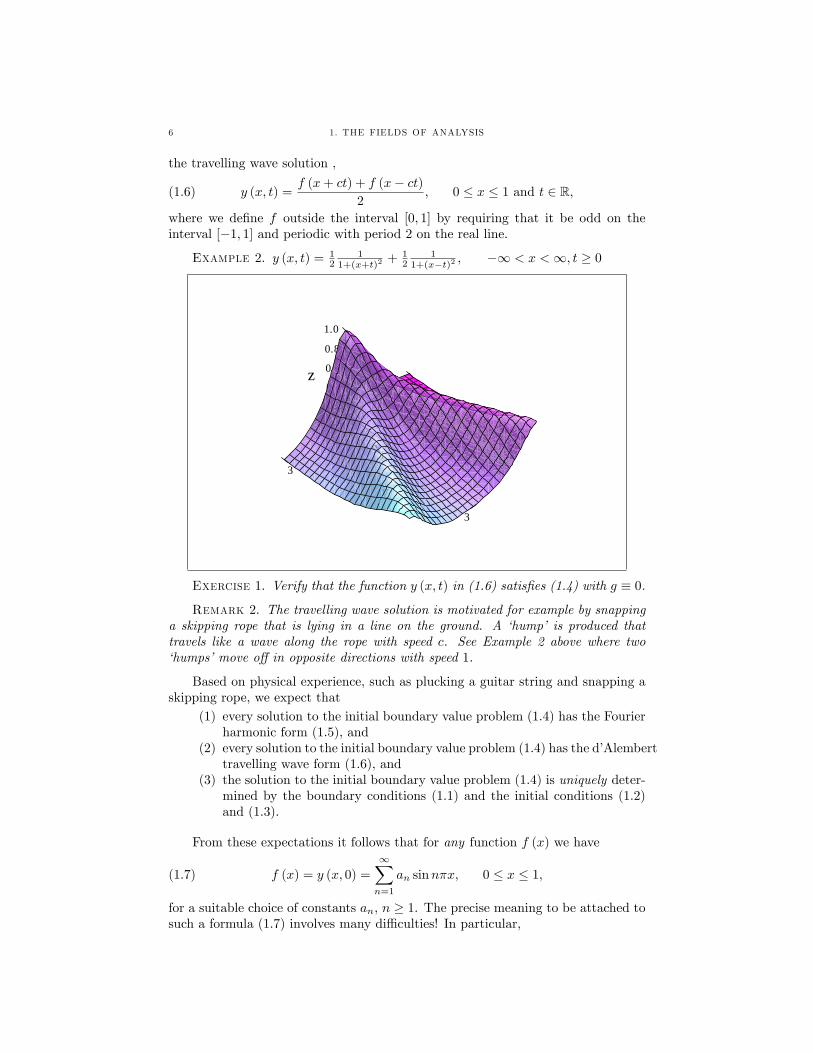
Example 1. y (x; t) = (sin 3�x) (cos 3�t)

1. A MODEL OF A VIBRATING STRING 5

1.0

1.5

0.5

z0.0

0.0

0.5

1.00.2

0.0

0.40.6

x0.81.0

y

0.5

1.0

Since the equations involved are linear we then have that

y (x; t) =NXn=1

an (sinn�x) (cosnc�t)

is a solution to (1.4) with initial conditions

f (x) =NXn=1

an sinn�x; 0 � x � 1;

g (x) = 0; 0 � x � 1:Presuming that we can take in�nite sums, we �nally obtain that the solution y (x; t)to the initial boundary value problem (1.4) with initial conditions

f (x) =1Xn=1

an sinn�x; 0 � x � 1;

g (x) = 0; 0 � x � 1;is given by the in�nite series of functions

(1.5) y (x; t) =1Xn=1

an (sinn�x) (cosnc�t) :

Remark 1. The Bernoulli decomposition is motivated for example by pluckinga guitar string. The fundamental note heard is that corresponding to n = 1, thestanding sine wave having one node that oscillates with frequency c

2 and amplitudea1. Corresponding to higher values of n are the harmonics having n nodes withfrequency nc

2 and amplitude an. See Example 1 above where the standing wavehaving 3 nodes has graph sin 3�x with frequency 3

2 and amplitude 1.

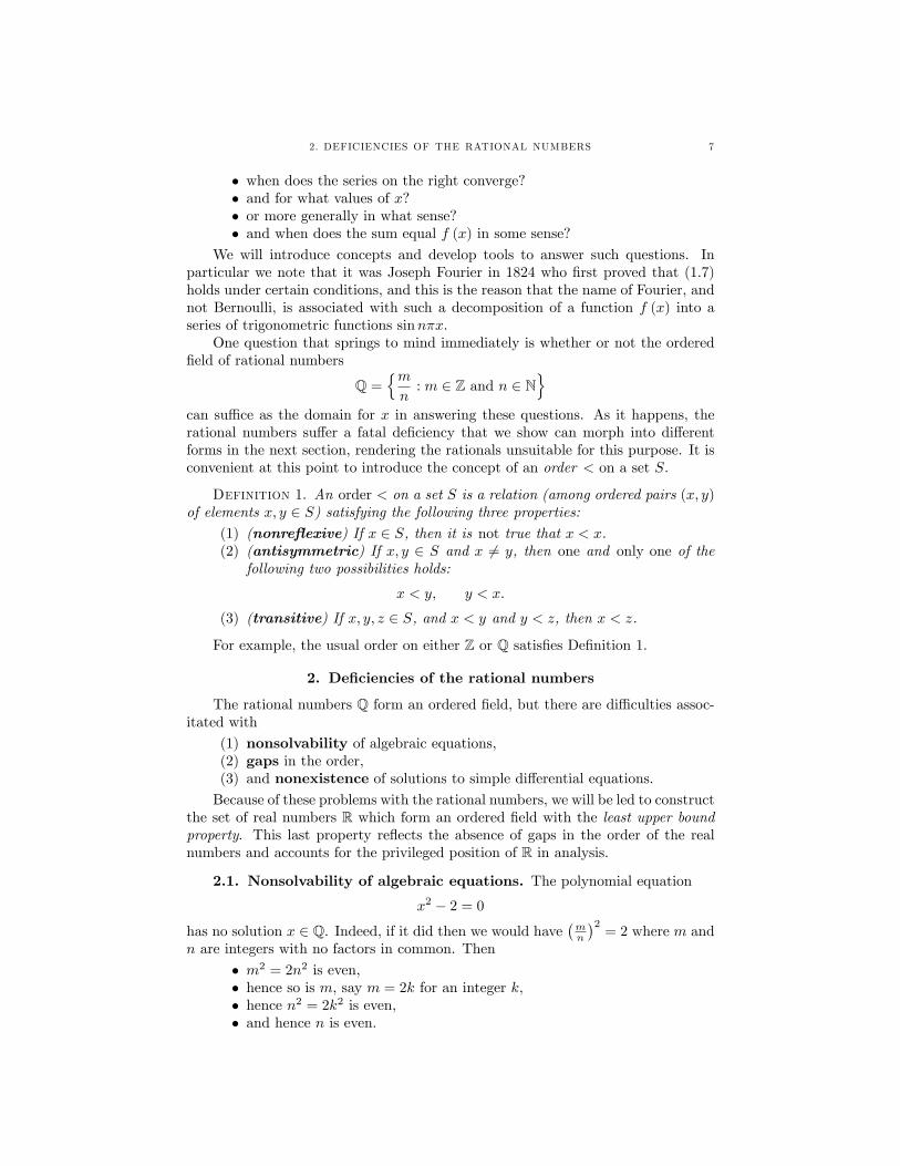
On the other hand, a much simpler solution to (1.4) with initial conditiong (x) = 0 for 0 � x � 1 was given by Jean Le Rond d�Alembert in 1747, namely


the travelling wave solution ,

(1.6) y (x; t) =f (x+ ct) + f (x� ct)

2; 0 � x � 1 and t 2 R;

where we de�ne f outside the interval [0; 1] by requiring that it be odd on theinterval [�1; 1] and periodic with period 2 on the real line.

Example 2. y (x; t) = 12

11+(x+t)2

+ 12

11+(x�t)2 ; �1 < x <1; t � 0

2y

10

x0

0.2

112

23

3

3

0.4z 0.6

0.8

1.0

Exercise 1. Verify that the function y (x; t) in (1.6) satis�es (1.4) with g � 0.

Remark 2. The travelling wave solution is motivated for example by snappinga skipping rope that is lying in a line on the ground. A �hump� is produced thattravels like a wave along the rope with speed c. See Example 2 above where two�humps�move o¤ in opposite directions with speed 1.

Based on physical experience, such as plucking a guitar string and snapping askipping rope, we expect that

(1) every solution to the initial boundary value problem (1.4) has the Fourierharmonic form (1.5), and

(2) every solution to the initial boundary value problem (1.4) has the d�Alemberttravelling wave form (1.6), and

(3) the solution to the initial boundary value problem (1.4) is uniquely deter-mined by the boundary conditions (1.1) and the initial conditions (1.2)and (1.3).

From these expectations it follows that for any function f (x) we have

(1.7) f (x) = y (x; 0) =1Xn=1

an sinn�x; 0 � x � 1;

for a suitable choice of constants an, n � 1. The precise meaning to be attached tosuch a formula (1.7) involves many di¢ culties! In particular,

2. DEFICIENCIES OF THE RATIONAL NUMBERS 7

� when does the series on the right converge?� and for what values of x?� or more generally in what sense?� and when does the sum equal f (x) in some sense?

We will introduce concepts and develop tools to answer such questions. Inparticular we note that it was Joseph Fourier in 1824 who �rst proved that (1.7)holds under certain conditions, and this is the reason that the name of Fourier, andnot Bernoulli, is associated with such a decomposition of a function f (x) into aseries of trigonometric functions sinn�x.

One question that springs to mind immediately is whether or not the ordered�eld of rational numbers

Q =nmn: m 2 Z and n 2 N

ocan su¢ ce as the domain for x in answering these questions. As it happens, therational numbers su¤er a fatal de�ciency that we show can morph into di¤erentforms in the next section, rendering the rationals unsuitable for this purpose. It isconvenient at this point to introduce the concept of an order < on a set S.

Definition 1. An order < on a set S is a relation (among ordered pairs (x; y)of elements x; y 2 S) satisfying the following three properties:

(1) (nonre�exive) If x 2 S, then it is not true that x < x.(2) (antisymmetric) If x; y 2 S and x 6= y, then one and only one of the

following two possibilities holds:

x < y; y < x:

(3) (transitive) If x; y; z 2 S, and x < y and y < z, then x < z.

For example, the usual order on either Z or Q satis�es De�nition 1.

2. De�ciencies of the rational numbers

The rational numbers Q form an ordered �eld, but there are di¢ culties assoc-itated with

(1) nonsolvability of algebraic equations,(2) gaps in the order,(3) and nonexistence of solutions to simple di¤erential equations.Because of these problems with the rational numbers, we will be led to construct

the set of real numbers R which form an ordered �eld with the least upper boundproperty. This last property re�ects the absence of gaps in the order of the realnumbers and accounts for the privileged position of R in analysis.

2.1. Nonsolvability of algebraic equations. The polynomial equation

x2 � 2 = 0has no solution x 2 Q. Indeed, if it did then we would have

�mn

�2= 2 where m and

n are integers with no factors in common. Then

� m2 = 2n2 is even,� hence so is m, say m = 2k for an integer k,� hence n2 = 2k2 is even,� and hence n is even.


This contradicts our assumption that m and n have no factors in common, andcompletes the proof that

p2 is not rational.

Alternatively, one can avoid divisibility and argue with inequalities to derive acontradiction as Fermat did:

�p2 = m

n where 0 < n < m < 2n,� 1 = 2� 1 =

�p2� 1

� �p2 + 1

�=�mn � 1

� �p2 + 1

�,

�p2 = 1

mn �1

� 1 = 2n�mm�n = m1

n1where n1 = m� n < n.

Thus we have shown that ifp2 can be represented as a quotient of positive

integers mn , then it can also be represented as a quotient of positive integers

m1

n1with n1 strictly smaller than n. This can be repeated as often as we wish, leadingto the contradiction that there are in�nitely many integers between 1 and n. Thistechnique is known as Fermat�s method of in�nite descent.

Remark 3. The equation x2+2 = 0 has no solution in Q either, in fact it hasno solution in the real numbers R. This prompts introduction of the set of complexnumbers C, which turns out to be an algebraically closed �eld containing the reals,i.e. every polynomial with real (even complex) coe¢ cients has a root in C. On theother hand, C is not an ordered �eld, which explains why so much of analysis beginswith the real �eld R.

2.2. Gaps in the order. The rational numbers can be decomposed into twodisjoint sets A and B with the properties that A has no largest element and B hasno smallest element, thus leaving a gap in the order. By this we mean that wecould insert a new element labelled X, @ or even

p2 into Q and extend the order

on Q to the larger set Q [ fXg by declaring p < X < q for all p 2 A and q 2 B.Because this extended order on Q[ fXg satis�es De�nition 1, we say that the setsA and B create a gap in the order of Q.

For example we can set

A =�p 2 Q : either p � 0 or p2 < 2

;(2.1)

B =�q 2 Q : q > 0 and q2 > 2

:

To see that A has no largest element, pick p 2 A. We may assume that p > 0, andsince every p in A is less than 2 we have 0 < p < 2. Set � = 2�p2

8 so that 0 < � < 14 .

Then

(p+ �)2= p2 + 2p� + �2

< p2 + 4� +1

4�

= p2 +1

2

�2� p2

�+1

32

�2� p2

�< p2 +

�2� p2

�= 2:

Thus p+ � > p and p 2 A. The proof that B has no smallest element is similar.

2.3. Nonexistence of solutions to di¤erential equations. The di¤eren-tial equation

y0 + xy3 = 0

3. THE REAL FIELD 9

has no solution on any open interval of rational numbers. Indeed, we can solve theequation in the real line by separating variables;

�12d

�1

y2

�=

dy

y3= �xdx = �1

2d�x2�;

1

y2= x2 + C;

y =1p

x2 + C:

No matter what choice of integration constant C is made, and what choice of interval(a; b) with rational numbers a < b, there are lots of rational numbers x 2 (a; b) forwhich y = 1p

x2+Cis not rational.

3. The real �eld

In regards to the problem of describing what is meant by the �continuity of a linesegment�, J. W. R. Dedekind published his famous construction of the real numbersusing Dedekind cuts in 1872. Some years earlier he had described his seminal ideain the following way "By this commonplace remark the secret of continuity is to berevealed", the idea in question being

� In any division of the points of the segment into two parts such that eachpoint belongs to one and only one class, and such that every point of theone class is to the left of every point in the other, there is one and onlyone point that brings about the division.

We present here a modi�cation of this idea due to Bertand Russell (born 1872,the year of Dedekind�s publication). Heuristically, following Russell, a Dedekindcut � � Q is a "left in�nite interval open on the right" of rational numbers thatis associated with the "real number" on the number line that marks its right handendpoint. More precisely, a cut � is a subset of Q satisfying (here p and q denoterational numbers)

� 6= ; and � 6= Q;(3.1)

p 2 � and q < p implies q 2 �;p 2 � implies there is q 2 � with p < q.

One can de�ne an ordered �eld structure on the set of cuts, which we identifyas the �eld R of real numbers, and prove that this ordered �eld has the famousLeast Upper Bound Property de�ned below. It is this property that evolves intothe critical Heine-Borel property of Euclidean space, namely that every closed andbounded subset is compact, and this property in turn ultimately permits the familiarexistence theorems for ordinary and partial di¤erential equations. We remark thata copy of the rational number �eld Q can be identi�ed inside the real �eld R ofDedekind cuts by associating to each r 2 Q the cut

� = (�1; r) � fp 2 Q : p < rg :

Alternatively, one can de�ne an ordered �eld structure on the set of equivalenceclasses of Cauchy sequences in Q, and this produces an ordered �eld isomorphic toR. We will construct the real numbers using Dedekind cuts at the end of thischapter, and leave the construction with Cauchy sequences to a later chapter. But


�rst we study some of the consequences of an ordered �eld with the least upperbound property. For this we introduce precise de�nitions of these concepts.

Definition 2. A �eld F is a set with two binary operations, called additionand multiplication, that satisfy the following three sets of axioms. We often writeF for the underlying set, x+ y for the operation of addition applied to x; y 2 F, andjuxtaposition xy for the operation of multiplication applied to x; y 2 F.

(1) Addition Axioms(a) (closure) x+ y 2 F for all x; y 2 F,(b) (commutativity) x+ y = y + x for all x; y 2 F,(c) (associativity) (x+ y) + z = x+ (y + z) for all x; y; z 2 F,(d) (additive identity) There is an element 0 2 F such that

0 + x = x for all x 2 F;(e) (inverses) For each x 2 F there is an element �x 2 F such that

x+ (�x) = 0:(2) Multiplication Axioms

(a) (closure) xy 2 F for all x; y 2 F,(b) (commutativity) xy = yx for all x; y 2 F,(c) (associativity) (xy) z = x (yz) for all x; y; z 2 F,(d) (multiplicative identity) There is an element 1 2 F such that

1x = x for all x 2 F;(e) (inverses) For each x 2 F n f0g there is an element 1x 2 F such that

x

�1

x

�= 1:

(3) Distributive Law

x (y + z) = xy + xz

for all x; y; z 2 F.

Example 3. The set of rational numbers Q is a �eld with the usual operationsof addition and multiplication. Another example is given by the �nite set of integers

Fp = f0; 1; 2; :::; p� 1g ;with addition and multiplication de�ned modulo p. This turns out to be a �eld ifand only if p is a prime number. Details are left to the reader.

All of the familiar algebraic identities that hold for the rational numbers, holdalso in any �eld. We state the most common such algebraic identities below leavingfor the reader some of the routine proofs.

Proposition 1. Let F be a set on which there are de�ned binary operations ofaddition and multiplication.

(1) The addition axioms imply(a) x+ y = x+ z =) y = z,(b) x+ y = x =) y = 0,(c) x+ y = 0 =) y = �x,(d) � (�x) = x.

(2) The multiplication axioms imply

3. THE REAL FIELD 11

(a) x 6= 0 and xy = xz =) y = z,(b) x 6= 0 and xy = x =) y = 1,(c) x 6= 0 and xy = 1 =) y = 1

x ,(d) x 6= 0 =) 1

1x

= x.

(3) The �eld axioms imply(a) 0x = 0,(b) x 6= 0 and y 6= 0 =) xy 6= 0,(c) (�x) y = � (xy) = x (�y),(d) (�x) (�y) = xy.

By way of illustration we prove the �nal equality (�x) (�y) = xy by a methodthat also establishes (1) (a) (c) (d) and (3) (a) (c) along the way (much shorter proofsalso exist). For this we begin with the additive cancellation property (1) (a): ifx+ y = x+ z then

y = 0 + y = (�x+ x) + y = �x+ (x+ y)= �x+ (x+ z) by assumption

= (�x+ x) + z = 0 + z = z:

Taking z = �x this gives (1) (c) (uniqueness of additive inverses), and since (�x)+x = 0, (1) (c) then gives x = � (�x), which is (1) (d). Next we note that(3.2) (�x) y + xy = (�x+ x) y = 0y = 0;where the �nal equality follows from applying additive cancellation (1) (a) to

0y + 0y = (0 + 0) y = 0y = 0y + 0:

By applying (1) (c) to (3.2) we obtain

(3.3) xy = � ((�x) y) :If we interchange x and y in (3.3) and use multiplicative commutativity, we alsoobtain

(3.4) xy = yx = � ((�y)x) = � (x (�y)) :Finally, with x replaced by �x and y replaced by �y in (3.3) we have

(�x) (�y) = � ((� (�x)) (�y)) = � (x (�y)) ;which when combined with (3.4) yields (�x) (�y) = xy as required.

Now we combine the �eld and order properties. By x > y we mean y < x.

Definition 3. An ordered �eld is a �eld F together with an order < on the setF where the �eld and order structures are connected by the following two additionalaxioms:

(1) x+ y < x+ z if x; y; z 2 F and y < z,(2) xy > 0 if x; y 2 F and both x > 0 and y > 0.

Example 4. The �eld of rational numbers Q is an ordered �eld with the usualorder, but for p a prime, there is no order on the �eld Fp that satis�es De�nition3.

All of the customary rules for manipulating inequalities in the rational numbershold also in any ordered �eld. We state the most common such properties below,without giving the routine proofs.


Proposition 2. The following hold in any ordered �eld.

(1) x > 0 if and only if �x < 0,(2) xy < xz if x > 0 and y < z,(3) xy > xz if x < 0 and y < z,(4) x2 > 0 if x 6= 0,(5) 1 > 0,(6) 0 < 1

y <1x if 0 < x < y.

Now we come to the most important property an ordered �eld can have, onethat is essential for the success of analysis, but is not satis�ed in the ordered �eldof rational numbers Q.

Definition 4. Let < be an order on a set S.

(1) We say that x 2 S is an upper bound for a subset E of S if

y � x for all y 2 E:

(2) We say that a subset E is bounded above if it has at least one upperbound.

(3) We say that x 2 S is the least upper bound for a subset E of S if x is anupper bound for E and if z is any other upper bound for E, then x � z.In this case we write

x = supE:

Clearly the least upper bound of a subset E, if it exists, is unique. Considerthe ordered set of rational numbers Q. Then 3 is an upper bound for the intervalE = [0; 3] = fx 2 Q : 0 � x � 3g, and so are �, 4 and 2100. In fact it is easy to seethat 3 is the least upper bound for [0; 3]. An example of a subset that has no leastupper bound is the semiin�nite interval [0;1) = fx 2 Q : 0 � x <1g, since it hasno upper bounds at all! A more substantial example of a bounded set that has noleast upper bound is the set A de�ned in (2.1).

There are corresponding de�nitions of lower bound, bounded below, greatestlower bound and inf E, whose formulations we leave to the reader.

Definition 5. An ordered set S has the Least Upper Bound Property if everysubset E of S that is bounded above has a least upper bound.

The ordered set of rational numbers Q fails to have this crucial property, asevidenced by the existence of the set A in (2.1). An example of a nontrivial orderedset with the Least Upper Bound Property is the set of all ordinal numbers equal toor less than the �rst uncountable ordinal.

Remark 4. If S has the Least Upper Bound Property, it also has the GreatestLower Bound Property: every subset E of S that is bounded below has a greatestlower bound. To see this, suppose E is bounded below and let L be the nonempty setof lower bounds. Then L is bounded above by every element of E and in particular� = supL exists. Now � = inf E follows from the following two facts:

(1) � 2 L since if < �, then cannot be an upper bound of L, hence =2 Esince every element of E is an upper bound of L. Thus � � x for everyx 2 E and so � 2 L.

(2) � =2 L if � > � since � is an upper bound of L.

3. THE REAL FIELD 13

It turns out that the only ordered �eld that has the Least Upper Bound Prop-erty is (up to isomorphism) the ordered �eld of real numbers R, which we have notyet constructed. Before embarking on the construction of the real numbers usingDedekind cuts, it will be useful to derive some consequences of the Least UpperBound Property in an ordered �eld. Just so we can be certain we are not workingin a vaccuum, we state the basic existence theorem whose proof is deferred to theend of this chapter.

Theorem 1. There exists an ordered �eld R having the Least Upper BoundProperty. Moreover, such a �eld is uniquely determined up to isomorphism (of or-dered �elds) and contains (an isomorphic copy of) the rational �eld Q as a sub�eld.

Assuming this existence theorem for the moment we derive some properties ofordered �elds with the Least Upper Bound Property. We note that we could alsoprove these properties by appealing to the explicit construction of the real numbersby Dedekind cuts below, but the approach used here is more streamlined in thatit avoids the complexities inherent in the construction of the reals. We begin withtwo familiar properties shared by the �eld of rational numbers.

Proposition 3. Let x; y 2 R.(1) (Archimedian property) If x > 0, then there is a positive integer n such

that nx > y.(2) (density of rationals) If x < y then there is p 2 Q such that x < p < y.

Proof : To prove assertion (1) by contradiction, let E = fnx : n 2 Ng. If (1)were false, then y would be an upper bound for E and consequently � = supEwould exist. Since x > 0, we would have �� x < � and thus that �� x could notbe an upper bound for E. But then there would be some nx greater than � � xand this gives

� = (�� x) + x< nx+ x

= (n+ 1)x 2 E;

which contradicts the assumption that � is an upper bound for E.To prove assertion (2), use assertion (1) to choose n 2 N such that n (y � x) > 1.

Use assertion (1) twice more to obtain integers m1 and m2 satisfying m1 > nx andm2 > �nx. Thus we have both

n (y � x) > 1 and �m2 < nx < m1.

Because m1� (�m2) > nx+(�nx) = 0, i.e. m1� (�m2) � 1, it follows that thereis an integer m lying between �m2 and m1 such that

m� 1 � nx < m:

Combining inequalities yields

nx < m � 1 + nx < ny;

and since n > 0 we obtain

x <m

n< y:


Similar reasoning can be used to obtain the existence of positive nth roots ofpositive numbers in an ordered �eld with the least upper bound property. Thisproperty is not shared by the �eld of rational numbers.

Proposition 4. (existence of nth roots) If x is a positive real number and nis a positive integer, then there exists a unique positive real number y satisfyingyn = x.

Sketch of the proof : Let E = fz 2 R : 0 < z and zn < xg. One can showthat E is nonempty and bounded above, hence y = supE exists. Using an argumentsimilar to that following (2.1) one can now show that each of the inequalities yn < xand yn > x leads to a contradiction, leaving only the possibility that yn = x. Fordetails of these arguments see page 10 of [3].

Note that supA =p2 where A is the set in (2.1).

Corollary 1. If x and y are positive real numbers and n is a positive integer,then x

1n y

1n = (xy)

1n .

Proof : By the commutativity of multiplication we have�x1n y

1n

�n=

�x1n y

1n

��x1n y

1n

�:::�x1n y

1n

�=

�x1n

��x1n

�:::�x1n

��y1n

��y1n

�:::�y1n

�=

�x1n

�n �y1n

�n= xy:

By the uniqueness assertion of Proposition 4 we then conclude that x1n y

1n = (xy)

1n .

4. The complex �eld

Property (4) of Proposition 2 on ordered �elds shows that there is no realnumber x satisfying the equation x2 = �1. To remedy this situation, we de�nethe complex �eld C to be the �eld obtained from the real �eld R by adjoining anabstract symbol i that is declared to satisfy the equation

(4.1) i2 = �1:Thus C consists of all expressions of the form

z = x+ iy; x; y 2 R;which can be identi�ed with the "points in the plane" by associating z = x+ iy 2 Cwith (x; y) 2 R � R in the plane. The �eld structure on C uses the multiplicationrule derived from (4.1) by

zw = (x+ iy) (u+ iv)(4.2)

=�xu+ i2yv

�+ i (xv + yu)

= (xu� yv) + i (xv + yu) ;where z = x+ iy and w = u+ iv. For the most part, straightforward calculationsshow that this multiplication and the usual addition derived from vectors in theplane R� R,

(x+ iy) + (u+ iv) = (x+ u) + i (y + v) ;

4. THE COMPLEX FIELD 15

satisfy the addition axioms, the multiplication axioms and the distributive law ofa �eld. Only the existence of a multiplicative inverse needs some elaboration. Forthis we de�ne

Definition 6. Suppose z = x+ iy 2 C. The complex conjugate z ofz is de�nedto be

z = x� iy:

Now

zz = (x+ iy) (x� iy) = x2 � (iy)2 + i fyx� xyg = x2 + y2;

and by Proposition 4, the nonnegative real numberpx2 + y2 exists and is unique.

By Pythagoras�theorem, px2 + y2 =

pzz

is the distance between the complex numbers 0 and z when they are viewed as thepoints (0; 0) and (x; y) in the plane. We de�ne

jzj =pzz; z 2 C;

called the absolute value of z, and note that for z 2 C n f0g, the multiplicativeinverse of z is given by z�1 = z

jzj2 since

z�z�1�= z

z

jzj2=

zz

jzj2=jzj2

jzj2= 1:

We now make three observations.

(1) An immediate consequence of property (4) of Proposition 2 is that there isno order on C that makes it into an ordered �eld with this �eld structure.

(2) It is a fundamental theorem in algebra, in fact it is called the fundamentaltheorem of algebra, that we do not need to adjoin any further solutionsof polynomial equations: every polynomial equation

zn + an�1zn�1 + :::+ a1z + a0 = 0

has a solution z in the complex �eld C. Here the coe¢ cients a0; a1; :::; an�1are complex numbers.

(3) If we associate z = x+ iy to the matrix�x �yy x

�, then this multiplica-

tion corresponds to matrix multiplication:

[z] [w] =

�x �yy x

� �u �vv u

�(4.3)

=

�xu� yv �xv � yuyu+ xv �yv + xu

�= [zw] :

Since the matrix�x �yy x

�= r

�cos � � sin �sin � cos �

�is dilation by the nonnegative number r =

px2 + y2 = jzj and rotation

by the angle � = tan�1 yx in the counterclockwise direction, we see that ifz has polar coordinates (r; �) and w has polar coordinates (s; �), then zw


has polar coordinates (rs; � + �). Finally we note that the inverse of the

matrix M =

�x �yy x

�is given by

M�1 =1

detM[coM ]

t=

1

x2 + y2

�x y�y x

�=

� xx2+y2

yx2+y2

� yx2+y2

xx2+y2

�;

which agrees with z�1 = zjzj2 =

xx2+y2 � i y

x2+y2 (M is the matrix repre-

sentation of the real linear map induced on R2 by the map of complexmultiplication on C = R2 by z = x+ iy).

Finally we give some simple properties of the complex conjugate and absolutevalue functions. If z = x+ iy we write Re z = x and Im z = y.

Proposition 5. Let z and jzj denote the complex conjugate and absolute valueof z.

(1) Suppose z; w 2 C. Then(a) z + w = z + w, (zw) = (z) (w) and z + z = 2Re z,(b) j0j = 0 and jzj > 0 unless z = 0,(c) jzj = jzj,(d) jzwj = jzj jwj,(e) jRe zj � jzj,(f) jz + wj � jzj+ jwj.

(2) (Cauchy-Schwarz inequality) Suppose z1; :::; zn 2 C and w1; :::; wn 2 C.Then��nXj=1

zjwj

��2

� jz1w1 + :::+ znwnj2 �

0@ nXj=1

jzj j21A0@ nX

j=1

jwj j21A :

Proof : Assertions (1) (a) (b) (c) (e) are easy. If z = x+ iy and w = u+ iv thenfrom (4.2),

jzwj2 = j(xu� yv) + i (xv + yu)j2

= (xu� yv)2 + (xv + yu)2

= x2u2 � 2xuyv + y2v2 + x2v2 + 2xvyu+ y2u2

=�x2 + y2

� �u2 + v2

�= jzj2 jwj2 ;

and now the uniqueness assertion of Proposition 4 proves (1) (d).Next we compute

jz + wj2 = (z + w) (z + w) = (z + w) (z + w)

= zz + zw + wz + ww

= jzj2 + 2Re (zw) + jwj2

� jzj2 + 2 jzwj+ jwj2

= jzj2 + 2 jzj jwj+ jwj2 = (jzj+ jwj)2 ;and the uniqueness assertion of Proposition 4 now proves (1) (f).

Finally, to obtain (2), set

Z =nXj=1

jzj j2 and W =nXj=1

jwj j2 and D =nXj=1

zjwj ;

4. THE COMPLEX FIELD 17

so that we must prove

(4.4) jDj2 � ZW:

If W = 0 then both sides of (4.4) vanish. Otherwise, we havenXj=1

jWzj �Dwj j2 =nXj=1

(Wzj �Dwj)�Wzj �Dwj

�= W 2

nXj=1

jzj j2 �WDnXj=1

zjwj �DWnXj=1

wjzj + jDj2nXj=1

jwj j2

= W 2Z �WDD �DWD � jDj2W

= W 2Z �W jDj2 =W�WZ � jDj2

�;

and since W > 0 we obtain

WZ � jDj2 = 1

W

nXj=1

jWzj �Dwj j2 � 0:

4.1. Euclidean spaces. For x = (x1; x2; :::; xn) 2 R � R � ::: � R � Rn, wede�ne

kxk =qx21 + x

22 + :::+ x

2n;

and interpret kxk as the distance from the point x to the origin 0 = (0; 0; :::; 0),which is reasonable since it agrees with Pythagoras� theorem. We call Rn theEuclidean space of dimension n. For z;w 2 Rn, we de�ne the dot product of z andw by

z �w = z1w1 + z2w2 + :::+ znwn =nXj=1

zjwj :

The Cauchy-Schwarz inequality, when restricted to real numbers, says that

jz �wj � kzk kwk ; z;w 2 Rn:

Remark 5. The proof of the Cauchy-Schwarz inequality given above is moti-vated by the fact that in a Euclidean space, the point on the line through 0 and wthat is closest to z is the projection Pz of z onto the line through 0 and w given by

Pz =

�z � wkwk

�w

kwk =z �wkwk2

w:

Then

kz� Pzk2 =nXj=1

��zj � z � wkwk2

wj

��2

=1

kwk4nXj=1

��kwk2 zj � (z �w)wj��2=

1

kwk4nXj=1

jWzj �Dwj j2 :


5. Dedekind�s construction of the real numbers

Recall that a Dedekind cut � is a subset of Q satisfying (3.1),

� 6= ; and � 6= Q;p 2 � and q < p implies q 2 �;p 2 � implies there is q 2 � with p < q.

We setR = f� : � is a cutg ;

and de�ne an order < and two binary operations, addition + and multiplication �,on the set R and then demonstrate that R satis�es the axioms for an ordered �eldwith the Least Upper Bound Property. We proceed in six steps, giving proofs onlywhen there is some trick involved, or the result is especially important. The lettersp; q; r; s; t always denote rational numbers and the Greek letters �; �; ; � alwaysdenote cuts. See pages 17-21 of [3] for the details.

Step 1 : De�ne � < � if � is a proper subset of �. Then (R; <) is an orderedset.

Step 2 : (R; <) has the Least Upper Bound Property.Proof : To see this, suppose that E is a nonempty subset of R that is bounded

above by � 2 R. De�ne =

[�2E

�:

One can now show that is a cut ( 6= ; since there exists � (6= ;) 2 E and then� � ; 6= Q since � � and � 6= Q; if p 2 , then there is � 2 E with p 2 �, andit follows that every q less than p is in � � and there is r in � � that is largerthan p), and clearly is then an upper bound for E since � � for all � 2 E.Moreover, is the least upper bound, written = supE, since any upper boundmust contain at least each set � 2 E. Note how easily we obtained the Least UpperBound Property by this construction!

Step 3 : If �; � 2 R, de�ne�+ � = fp+ q : p 2 � and q 2 �g :

Also set� = fp 2 Q : p < 0g :

Then � + � and � are cuts and using � as the additive identity 0, the AdditionAxioms for a �eld hold. In fact more is true: if � is a cut and � is any nonemptyset that is bounded above, then �+ � is a cut.

Proof : If p = r + s 2 � + � and q < p, then q = (q � p+ r) + s 2 � + �since q � p + r < r and � is a cut. Furthermore, there is t 2 � with t > r and sot + s 2 � + � with t + s > r + s = p. Obviously � is a cut. Next, � + � � � andif p 2 �, then there is r 2 � with r > p and so p = r + (p� r) 2 � + �, and thisshows that �+ � = � for all � 2 R. It requires only a bit more e¤ort to show thatthe inverse of � 2 R is given by the set

�� fp 2 Q : there exists r > 0 such that � p� r =2 �g :Indeed, it is not too hard to show that �� is a cut. To see the more delicate factthat

(5.1) �+ (��) = �;

5. DEDEKIND�S CONSTRUCTION OF THE REAL NUMBERS 19

we �rst note that � + (��) � � since if q 2 � and r 2 ��, then �r =2 �, henceq < �r, hence q + r < 0. Conversely, pick s 2 � and set t = � s

2 > 0. By theArchimedian property of the rational numbers Q, there is n 2 N such that

nt 2 � but (n+ 1) t =2 �:Set p = � (n+ 2) t.

Remark 6. It is helpful at this point to suppose that � corresponds to a pointon the line to the right of 0, and to draw the players in the proof from left to righton the line:

p < � (n+ 1) t < �� < �nt < �t < 0 < t < nt < � < (n+ 1) t < �p:

Now p 2 �� since �p� t = (n+ 1) t =2 �. Since nt 2 � we thus haves = �2t = nt+ p 2 �+ (��) :

This proves that � � �+ (��) and completes the proof of (5.1).Step 4 : If �; �; 2 R and � < , then �+ � < �+ .Proof : This is easy to prove using the cancellation law for addition in Propo-

sition 1 (1) (a). Indeed, when cuts are considered as subsets of rational numbers,we clearly have �+� � �+ . If we had equality �+� = �+ , then Proposition 1(1) (a) shows that � = , a contradiction. Note that Proposition 1 (1) applies heresince we have shown in Step 3 that the addition axioms hold.

Step 5 : If �; � > �, de�ne

� � � = fp 2 Q : p � qr for some choice of

q 2 � with q > 0 and r 2 � with r > 0g :For general �; � 2 R, de�ne � �� appropriately. Then (R; <;+; �) is an ordered �eldwith the Least Upper Bound Property.

Proof : The proof of the multiplication axioms is somewhat bothersome dueto the di¤erent de�nitions of product � � � according to the signs of � and �. Weomit the remaining tedious details in the proof of Step 5.

Step 6 : To each q 2 Q we associate the set� (q) � fp 2 Q : p < qg :

Then � (q) is a cut and

� (r + s) = � (r) + � (s) ;

� (rs) = � (r) � � (s) ;� (r) < � (s)() r < s:

Thus the map � : Q! R is an ordered �eld isomorphism from the rational numbersQ into the real numbers R, and this is the sense in which we mean that the realnumbers R contain a copy of the rational numbers Q.

Remark 7. One might reasonably ask why in the de�nition of cut (3.1) we hadto include the third condition requiring the cut to have no largest element:

p 2 � implies there is q 2 � with p < q:

However, without this condition, there are additional cuts, namely those with alargest rational element:

r� � fp 2 Q : p � rg ; for r 2 Q:


We refer to these additional cuts as closed cuts, and to the original cuts as opencuts. A cut that is either closed or open is said to be a generalized cut. Suppose weextend the de�nition of addition to generalized cuts in the standard way by takingall possible sums of pairs, one element from each cut. The key property to observethen is that �+� is an open cut provided at least one of � and � is open (see Step3 above). Thus the usual zero element 0 can no longer serve as the additive identityfor the set of generalized cuts. It is not hard to see however that the closed cut

0� � fp 2 Q : p � 0ghas the required additive identity property 0�+� = � for all generalized cuts � - infact 0� is the only generalized cut with this property. Now comes the problem. Anopen cut � cannot have an additive inverse since the result of adding any generalizedcut to � must also be open - and in particular cannot equal the closed cut 0�.

CHAPTER 2

Cardinality of sets

Dedekind was the �rst to de�ne an in�nite set as one to which the paradoxesof Galileo and Bolzano applied (there are as many perfect squares as there areintegers; there are as many even integers as there are integers; and there are asmany points in the interval [0; 1] as there are in [0; 2]):

� A system S is said to be in�nite if it is similar to a proper part of itself;in the contrary case S is said to be a �nite system.

In other words, a set S was de�ned to be in�nite by Dedekind if there existeda one-to-one correspondence between S and a proper subset of itself. However,Dedekind�s de�nition gave no hint that there might be di¤erent �sizes�of in�nity,and the creation of this revolutionary concept had to await the imagination of GeorgCantor.

Definition 7. Two sets A and B are said to have the same cardinality or aresaid to be equivalent, written A � B, if there is a one-to-one onto map ' : A! B.Let n 2 N. A set E is said to have cardinality n if it is equivalent to the set

Jn � f1; 2; 3; :::; n� 1; ng ;

in which case it is said to be �nite. A set E is said to be countable if it is equivalentto the set of natural numbers N. If a set is neither �nite nor countable, it is saidto be uncountable.

The relation � of having the same cardinality is an equivalence relation, mean-ing that it satis�es

(1) (re�exivity) A � A,(2) (symmetry) A � B =) B � A,(3) (transitiviy) A � B and B � C =) A � C.

These equivalence classes are called cardinal numbers since they measure thesize of sets up to bijections. Cantor showed at least two surprising results regardingcardinality: �rst, that the set of rational numbers is countable and second, thatthe set of real numbers is uncountable. Both demonstrations involved a notion ofdiagonalization.

21

22 2. CARDINALITY OF SETS

To show that the rational numbers Q are countable, Cantor arranged the pos-itive rational numbers Q+ in an in�nite matrix

�mn

�1m;n=1

;2666666666664

11

12

13

14 � � �

% % % %21

22

23

24 � � �

% % %31

32

33

34 � � �

% %41

42

43

44 � � �

... %...

......

. . .

3777777777775;

and then de�ned a map s : N ! Q+ by following the upward sloping diagonals insuccession, taking only those fractions that have not yet appeared:

s (1) =1

1;

s (2) =2

1; s (3) =

1

2;

s (4) =3

1; s (5) =

1

3(2

2= s (1) was skipped);

s (6) =4

1; s (7) =

3

2; s (8) =

2

3; s (9) =

1

4;

s (10) =5

1; s (11) =

1

5(4

2= s (2) ;

3

3= s (1) ;

2

4= s (3) were all skipped);

...

Clearly the map s is one-to-one and onto, thus demonstrating that N � Q+. Itis now a simple matter to use s to construct a one-to-one onto map t : N ! Q(exercise: do this!) that shows N � Q.

To show that the real numbers are uncountable, we begin with a famous paradoxof Russell. De�ne a set S by the rule

a 2 S , a =2 a;

i.e. S consists of all sets a that are not members of themselves. Then we have thefollowing paradox:

� If S 2 S, then by the very de�nition of S it must be the case that S =2 S,a contradiction.

� On the other hand if S =2 S, then by the very de�nition of S it must bethe case that S 2 S, again a contradiction.

One way out of this paradox is to note that we have never seen a set a that is amember of itself. Thus we expect that S is actually the collection of all sets. If wesimply disallow the collection of all sets as a set, Russell�s paradox dissolves. Thistype of thinking eventually led to the Zermelo-Frankel set theory in use today.

Russell�s paradox suggests the following proof that the power set

P (N) � fE : E � Ng

of the natural numbers, i.e. the set of all subsets of N, is uncountable. Indeed,assume in order to derive a contradiction, that P (N) is countable. Then we can

2. CARDINALITY OF SETS 23

list all the elements of P (N) = fEmg1m=1 in a vertical column:26664E1

E2

E3

...

37775 :Now each subset Em is uniquely determined by its characteristic function, i.e. thesequence fsmn g

1n=1 = fsm1 ; sm2 ; sm3 ; :::g of 0�s and 1�s de�ned by

smn =

�0 if n =2 Em1 if n 2 Em

:

Replace each subset Em in the vertical column by the in�nite row of 0�s and 1�sdetermined by fsmn g

1n=1 to get an in�nite matrix of 0�s and 1�s:26664

s11 s12 s13 � � �s21 s22 s23s31 s32 s33...

. . .

37775 :Now consider the anti-diagonal or Russell sequence frng1n=1 given by(0.2) rn = 1� snn:This is a sequence of 0�s and 1�s that is not included in the list26664

�s1n1n=1�

s2n1n=1�

s3n1n=1...

37775 ;since for each m, the sequences fsmn g

1n=1 and frng

1n=1 di¤er in the m

th entry:smm 6= rm by (0.2). Thus the set E = fn : rn = 1g whose characteristic function isthe sequence frng1n=1 satis�es

n 2 E , rn = 1, snn = 0, n =2 En,and hence is the set of n such that n is not a member of En (reminiscent of Russell�sparadox). It follows that E is not included in the list fEmg1m=1. This contradictionshows that the power set P (N) is uncountable. Equivalently, this shows that theset of all sequences consisting of 0�s and 1�s is uncountable.

To see from this that the real numbers are uncountable, express each realnumber s in the interval (0; 1] as a binary fraction

s =s12+s222+ :::+

sn2n+ ::: � 0:s1s2:::sn:::

where the sequence fsng1n=1 does not end in an in�nite string of 0�s. Since the setof such fractions is uncountable (in fact its equivalence with P (N) follows from theargument above with just a little extra work), we conclude that the interval (0; 1]is uncountable, and then so is R. We will return to this argument later.

We now turn to the task of making the previous arguments more rigorous. Webegin with a careful de�nition of �sequence�.

24 2. CARDINALITY OF SETS

Definition 8. A sequence is a function f de�ned on the natural numbers N.If f (n) = sn for all n 2 N, the values sn are called the terms of the sequence, andwe often denote the sequence f by fsng1n=1 or even fs1; s2; s3; :::g.

Thus we may regard a countable set as the range of a sequence of distinctterms, and in fact we used this point of view when we assumed above that P (N)was countable and then listed the elements of P (N) in a vertical column. The nextlemma proves the intuitive fact that �countable is the smallest in�nity�.

Lemma 1. Every in�nite subset of a countable set is countable.

Proof : Suppose A is countable and E is an in�nite subset of A. RepresentA as the range of a sequence fang1n=1 of distinct terms, and de�ne a sequence ofintegers fnkg1k=1 as follows:

n1 = min fn 2 N : an 2 Eg ;n2 = min fn > n1 : an 2 Eg ;n3 = min fn > n2 : an 2 Eg ;

...

nk = min fn > nk�1 : an 2 Eg ; k � 4;...

Since E is in�nite, nk is de�ned for all k 2 N. It is now clear that E = fankg1k=1,

and so E is countable.

Corollary 2. A subset of a countable set is at most countable, i.e. it is eithercountable or �nite.

The next two theorems generalize the countability of the rational numbers andthe uncountability of the real numbers respectively. They are proved by the samediagonalization procedures used above, and their proofs are left to the reader.

Theorem 2. Let fEng1n=1 be a sequence of countable sets. Then S �S1n=1En

is countable.

The above theorem says that a countable union of countable sets is countable.Note that the sets En may overlap, but not so much as to make the union �nite,since their union S contains E1, and hence S is not �nite. As an immediate corollarywe may replace �countable�with �at most countable�.

Corollary 3. An at most countable union of at most countable sets is at mostcountable.

Theorem 3. Let A be the set of all sequences whose terms are either 0 or 1.Then A is uncountable.

Here is one more result on countable sets that is easily proved by induction.

Proposition 6. Let A be countable and consider the n-fold product set An =A�A� :::�A de�ned by

An � f(a1; a2; :::; an) : ai 2 A for 1 � i � ng :Then An is countable.

2. CARDINALITY OF SETS 25

Proof : Clearly A1 � A is countable. We now proceed by induction on n andassume that An�1 is countable. Assuming that n > 1 we have

An =�(b; c) : b 2 An�1 and c 2 A

:

Now for each �xed c 2 A, the set of pairs�(b; c) : b 2 An�1

is equivalent to An�1

which is countable by our induction assumption. Since A is countable, we thus seethat An is a countable union of countable sets, hence countable by Theorem 2.

CHAPTER 3

Metric spaces

There is a notion of distance between numbers in both the rational �eld Q andin the real �eld R given by the absolute value of the di¤erence of the numbers:

dist (p; q) = jp� qj ; p; q 2 Q;dist (x; y) = jx� yj ; x; y 2 R:

Motivated by Pythagoras�theorem, this can be extended to complex numbers C by

dist (z; w) = jz � wj =q(x� u)2 + (y � v)2;

for z = x+ iy and w = u+ iv in C;

and even to points or vectors in Euclidean space:

dist (x;y) � kx� yk =

vuut nXk=1

(xk � yk)2;

for x = (x1; :::; xn) and y = (y1; :::; yn) in Rn.

It will eventually be important to de�ne a notion of distance between functions, forexample if f and g are continuous functions on the unit interval [0; 1], then we willde�ne

dist (f; g) = sup fjf (x)� g (x)j : 0 � x � 1g :

Of course at this point we don�t even know if this supremum is �nite, i.e. if theset in braces is bounded above, or if it is, whether or not this de�nition satis�esproperties that we would expect of a �distance function�. Thus we begin by settingdown in as abstract a setting as possible the properties we expect of a distancefunction.

Definition 9. A set X together with a function d : X �X ! [0;1) is said tobe a metric space, and d is called a metric or distance function on X, provided:

(1) d (x; x) = 0,(2) d (x; y) > 0 if x 6= y,(3) d (x; y) = d (y; x) for all x; y 2 X,(4) (triangle inequality) d (x; z) � d (x; y) + d (y; z) for all x; y; z 2 X.

To be precise we often write a metric space as a pair (X; d). Examples of metricspaces include R, C and Rn with the distance functions given above. The triangleinequality holds in C by Proposition 5 (1) (f). To prove that the triangle inequalityholds in Rn we can use the Cauchy-Schwarz inequality just as we did in the proof

27

28 3. METRIC SPACES

of Proposition 5 (1) (d):

dist (x; z)2= kx� zk2 =

nXk=1

(xk � zk)2 =nXk=1

(xk � yk + yk � zk)2

=nXk=1

(xk � yk)2 + 2nXk=1

(xk � yk) (yk � zk) +nXk=1

(yk � zk)2

� kx� yk2 + 2 kx� yk ky � zk+ ky � zk2

= (kx� yk+ ky � zk)2 = (dist (x; y) + dist (y; z))2 :

Taking square roots we obtain

(0.3) dist (x; z) = kx� zk � kx� yk+ ky � zk = dist (x; y) + dist (y; z) :

We can also consider di¤erent metrics on Rn such as taxicab distance:

dtaxi (x; y) = max fjxk � ykj : 1 � k � ng :

This is the shortest distance a taxi must travel to get from x to y if the taxi isrestricted to proceed only vertically or horizontally, as is the case in most citiesbuilt around a rectangular grid of streets. It is not too hard an exercise to provethat (Rn; dtaxi) is a metric space, i.e. that dtaxi satis�es the axioms in De�nition 9on the set Rn.

An important method of constructing new metric spaces from known metricspaces is to consider subsets. Indeed, if (X; d) is a metric space and Y is any subsetof X, then (Y; d) is also a metric space, as is immediately veri�ed by restricting thepoints x; y; z in De�nition 9 to lie in the subset Y . For example the open unit disk

D = fz 2 C : dist (0; z) < 1g

=n(x; y) 2 R2 :

px2 + y2 < 1

ois a metric space with the metric d (z; w) = jz � wj. Note that the open unit diskin the complex plane C coincides with the open unit disk in the Euclidean planeR2.

The concept of a ball in a metric space is central to the further development ofthe theory of metric spaces.

Definition 10. Let (X; d) be a metric space and suppose x 2 X and r > 0.The ball B (x; r) with center x and radius r is de�ned to be the set of all pointsy 2 X at a distance less than r from x:

B (x; r) = fy 2 X : d (x; y) < rg :

One can easily verify that the collection of balls fB (x; r)gx2X;r>0 in a metricspace (X; d) satis�es the following six properties for all x; y 2 X:

(1)Tr>0B (x; r) = fxg,

(2)Sr>0B (x; r) = X,

(3) If 0 < r � s, then B (x; r) � B (x; s)(4) If y 2 B (x; r), then x 2 B (y; r),(5) The set fr > 0 : y 2 B (x; r)g has no least element,(6) If B (x; r) \B (y; s) 6= ;, then y 2 B (x; r + s).

1. TOPOLOGY OF METRIC SPACES 29

While we will not need to know this, the six properties above characterize ametric space in the following sense. Suppose that fB (x; r)gx2X;r>0 is a collectionof subsets of a set X that satisfy the six properties listed above. De�ne

d (x; y) = inf fr > 0 : y 2 B (x; r)g ; for all x; y 2 X:Then it is not too hard to show that d maps X � X into [0;1) and satis�es thefour properties in De�nition 9, i.e. d de�nes a metric or distance function on X.Moreover, one can prove that B (x; r) = fy 2 X : d (x; y) < rg for all x 2 X andr > 0, so that the initial collection of subsets fB (x; r)gx2X;r>0 are precisely thecollection of balls corresponding to the metric d.

1. Topology of metric spaces

The notion of an open set is at the center of the subject of topology.

Definition 11. Let (X; d) be a metric space and suppose G is a subset of X.Then G is open if for every point x in G there is a positive radius r such that theball B (x; r) is contained in G:

B (x; r) � G:

We see that the empty set ; is open by default (there is nothing to check). Theset X is open since

B (x; 1) � X; for all x 2 X:Any positive number would do in place of 1 as the radius above. One suspects thatballs themselves are open sets, but this needs a proof which relies heavily on thetriangle inequality.

Lemma 2. Let B be a ball in a metric space (X; d). Then B is open.

Proof : Suppose that B = B (y; s) and that x 2 B. Then by De�nition 10 wehave d (y; x) < s. Set

r = s� d (x; y) > 0:We claim that the ball B (x; r) with center x and radius r is contained in B (y; s).Draw a picture before proceeding! Indeed, if z 2 B (x; r) then by De�nition 10we have d (x; z) < r. Now we use the fact that the metric d satis�es the triangleinequality in De�nition 9 to compute that

d (y; z) � d (y; x) + d (x; z) < d (x; y) + r = s:

This shows that z 2 B (y; s) for every z 2 B (x; r), i.e.B (x; r) � B (y; s) :

Thus we have veri�ed the condition that for every point x in B (y; s) there is apositive radius r = rx (depending on the point x we chose in B (y; s)) such that theball B (x; rx) is contained in B (y; s). This proves that B (y; s) is an open set.

Exercise 2. Consider the Euclidean space R2.(1) Show that the inside of the ellipse,

G =�(x; y) 2 R2 : 4x2 + y2 < 1

;

is open. Hint: If P � (x; y) 2 G, then the ball B (P; r) is contained in Gif

r =1

2

�1�

p4x2 + y2

�:

30 3. METRIC SPACES

Indeed, if Q = (u; v) 2 B (P; r), then (0.3) yieldsq(2u)

2+ v2 �

q(2u� 2x)2 + (v � y)2 +

q(2x)

2+ y2

� 2

q(u� x)2 + (v � y)2 +

q(2x)

2+ y2

< 2r +

q(2x)

2+ y2 = 1:

(2) On the other hand, show that the corresponding set

F =�(x; y) 2 R2 : 4x2 + y2 � 1

;

de�ned with � in place of <, is not an open set. Hint: The point P �(0; 1) 2 F but for every r > 0 the ball B (P; r) contains the point

�0; 1 + r

2

�which is not in F .

We declare a subset F of a metric space X to be closed if the complementF c � X nF of F is an open set. For example, the set F in Exercise 2 (2) is closed,but the set G in Exercise 2 (1) is not closed.

Caution: A set may be neither open nor closed, such as the subset [0; 1) ofR. Moreover, a set may be simultaneously open and closed, such as boththe empty set ; and the entire set X in any metric space X.

Proposition 7. Let X be a metric space.

(1) If fG�g�2A is a collection of open subsets, thenS�2AG� is open,

(2) If fF�g�2A is a collection of closed subsets, thenT�2A F� is closed,

(3) If fGkgnk=1 is a �nite collection of open subsets, thenTnk=1Gk is open,

(4) If fFkgnk=1 is a �nite collection of closed subsets, thenSnk=1 Fk is closed.

Proof : Suppose that G� is open for each � and let x 2S�2AG�. Then

x 2 G� for some � and since G� is open, there is a ball B (x; r) � G� �S�2AG�,

which shows thatS�2AG� is open. Next suppose that F� is closed for each � and

note that if G� = (F�)c, then G� is open for each � and so

S�2AG� is open by

part (1). Thus from de Morgan�s laws we have that \�2A

F�

!c=[�2A

(F�)c=[�2A

G�

is open, soT�2A F� is closed by de�nition.

Now suppose that Gk is open for 1 � k � n and that x 2Snk=1Gk. Then there

is rk > 0 such that B (x; rk) � Gk for 1 � k � n. It follows that if we set

r = min frkgnk=1 ;then r > 0 (this is where we use that the collection fGkgnk=1 is �nite) and

B (x; r) � B (x; rk) � Gk; 1 � k � n:

Thus B (x; r) �Tnk=1Gk and this shows that

Tnk=1Gk is open. Finally, if Fk is

closed for 1 � k � n, then Gk = (Fk)c is open and so

n[k=1

Fk

!c=

n\k=1

(Fk)c=

n\k=1

Gk

is open by part (3). ThusSnk=1 Fk is closed by de�nition.

1. TOPOLOGY OF METRIC SPACES 31

1.1. Subspaces. Recall that if Y is a subset of a metric space X, then wemay view Y as a metric space in its own right, with metric given by that of Xrestricted to Y � Y . The metric space (Y; d) is then called a subspace of (X; d),even though there is no linear structure on X. Note that if y 2 Y and r > 0, thenthe ball BY (y; r) in the metric space Y satis�es

(1.1) BY (y; r) = fz 2 Y : d (y; z) < rg = BX (y; r) \ Y;

where BX (y; r) is the ball centered at y with radius r in the metric space X. Thusif E is a subset of Y , it can be considered as a subset of either the metric space Yor the metric space X. Clearly the notions of E being open or closed depend onwhich space is considered the ambient space. For example, if

E =

�(x; y) 2 R2 : dist

��0;1

2

�; (x; y)

�� 1

2

�n f(1; 0)g

is the ball center�0; 12�with radius 1

2 together with its "boundary" except for thepoint (1; 0), then we have

E � D � R2:Now one can show that E is a closed subset relative to the metric space D, but it isneither open nor closed as a subset relative to the metric space R2. Exercise: provethis!

On the other hand, (1.1) provides the following simple connection between theopen subsets relative to X and the open subsets relative Y .

Theorem 4. Let Y be a subset of a metric space X. Then a subset E of Y isopen relative to Y if and only if there exists a set G open relative to X such that

E = G \ Y:

Proof : Suppose that E is open relative to Y . Then for each p 2 E there is apositive radius rp such that BY (p; rp) � E. Now set

G =[p2E

BX (y; rp) ;

where we note that we are using balls BX relative to X. Clearly G is open relativeto X by Lemma 2 and Proposition 7 (1). From (1.1) we obtain

G \ Y =[p2E

fBX (y; rp) \ Y g =[p2E

BY (p; rp) ;

and the �nal set is equal to E since p 2 BY (p; rp) � E for each p 2 E.Conversely, suppose G is open relative to X and E = G\Y . Then given p 2 E,

there is rp > 0 such that BX (p; rp) � G. From (1.1) we thus obtain

BY (p; rp) = BX (y; rp) \ Y � G \ Y = E;

which shows that E is open relative to Y .

1.2. Limit points. In order to de�ne the notion of limit of a function lateron, we will need the idea of a limit point of a set. A deleted ball B0 (p; r) in a metricspace is the ball B (p; r) minus its center p, i.e. B0 (p; r) = B (p; r) n fpg.

32 3. METRIC SPACES

Definition 12. Suppose (X; d) is a metric space and that E is a subset of X.We say that p 2 X is a limit point of E if every deleted ball centered at p containsa point of E:

B0 (p; r) \ E 6= ; for all r > 0:

Note the following immediate consequence of this de�nition:

� if p is a limit point of E then every deleted ball B0 (p; r) contains in�nitelymany points of E,

and so in particular E must be in�nite in order to have any limits points at all.Indeed, if B0 (p; r)\E = fxjgnj=1 contains only n points, let s = min fd (p; xj)g

nj=1.

Then s > 0 and B (p; s) doesn�t contain any of the points fxjgnj=1. Thus we havethe contradiction B0 (p; s) \ E = ;.

Limit points are closely related to the notion of a closed set.

Proposition 8. A set F is closed in a metric space if and only if it containsall of its limit points.

Proof : Suppose �rst that x is a limit point of F . Then in particular, B (x; r)\Fis nonempty for all r > 0, and so no ball B (x; r) centered at x is contained in F c.If F is closed, then F c is open and it then follows that x =2 F c. Thus x 2 F andwe have shown that a closed set F contains all of its limit points.

Conversely, suppose that F contains all of its limit points. Pick x 2 F c. Sincex is not a limit point of F , there is a deleted ball B0 (x; r) that does not intersectF . But x =2 F as well so that B (x; r) does not intersect F . Hence B (x; r) � F c

and this shows that F c is open, and thus that F is closed.

Definition 13. If E is a subset of a metric space X, we de�ne E0 (the derivedset of E) to be the set of all limit points of E, and we de�ne E (the closure of E)to be E [ E0

, the union of E and all of its limit points.

As a corollary to Proposition 8 we obtain the following basic theorem for themetric space R.

Theorem 5. Suppose that E is a nonempty subset of the real numbers R thatis bounded above, and let supE be the least upper bound of E. Then supE is in E,and supE 2 E if E is closed.

Proof : Since the real numbers R have the Least Upper Bound Property, z �supE exists and satis�es the property that if y < z, then y is not an upper boundof E, hence there exists x 2 E with y < x � z. It follows that B (z; r) \ E 6= ; forall r > 0 upon taking y = z � r in the previous argument. Thus either z 2 E � Eor if not, then

B0 (z; r) \ E 6= ; for all r > 0;

in which case z is a limit point of E, hence z 2 E0 � E. Finally, Proposition 8shows that z 2 E if E is closed.

One might wonder if the set E contains limit points not in E, or roughlyspeaking, if taking limit points of limit points yields new points. The answer is no,and in fact not only is E closed, it is the smallest closed set containing E.

2. COMPACT SETS 33

Proposition 9. If E is a subset of a metric space X, then

(1.2) E =\fF � X : F is closed and E � Fg ;

and E is the smallest closed set containing E.

Proof : Denote the right hand side of (1.2) by E . Then E is a closed set byProposition 7 (2). Thus by its very de�nition, it is the smallest closed set containingE, i.e. every other closed set F containing E contains E . Now E � E since byProposition 8, every closed set F containing E also contains all the limit points E0

of E.On the other hand, if x =2 E, then there exists some r > 0 such that

B (x; r) \ E = ;:Now B (x; r)

c is closed since B (x; r) is open by Lemma 2. Moreover B (x; r)c

contains E and so is a candidate for the intersection de�ning E . This shows thatE � B (x; r)

c and in particular that x =2 E . This proves that E � E and completesthe proof of Proposition 9.

Lemma 3. E0 is closed.

Proof : Suppose that z 2 (E0)0 and r > 0. Then there is y 2 B0 (z; r) \ E0.Let s = min fd (z; y) ; r � d (z; y)g. Then s > 0 and there is x 2 B0 (y; s) \ E. Nowx 6= z since otherwise s � d (z; y) = d (x; y) < s, a contradiction. Also,

d (z; x) � d (z; y) + d (y; x) < d (z; y) + s � r:

Thus x 2 B0 (z; r) \ E and this shows that z 2 E0 as required.

2. Compact sets

Now we come to the single most important property that a subset of a metricspace can have, namely compactness. In a sense, compact subsets share the mostimportant topological properties enjoyed by �nite sets. It turns out that the mostbasic of these properties is rather abstract looking at �rst sight, but arises so of-ten in applications and subsequent theory that we will use it as the de�nition ofcompactness. But �rst we introduce some needed terminology.

Let E be a subset of a metric space X. A collection G � fG�g�2A of subsetsG� of X is said to be an open cover of E if

each G� is open and E �[�2A

G�:

A �nite subcover (relative to the open cover G of E) is a �nite collection fG�kgnk=1

of the open sets G� that still covers E:

E �n[k=1

G�k :

For example, the collection G =��

1n ; 1 +

1n

�1n=1

of open intervals in R form an

open cover of the interval E =�18 ; 2�, and

��1n ; 1 +

1n

�8n=1

is a �nite subcover.Draw a picture! However, G is also an open cover of the interval E = (0; 2) forwhich there is no �nite subcover since 1

m =2�1n ; 1 +

1n

�for all 1 � n � m.

Definition 14. A subset E of a metric space X is compact if every open coverof E has a �nite subcover.

34 3. METRIC SPACES

Example 5. Clearly every �nite set is compact. On the other hand, the interval(0; 2) is not compact since G =

��1n ; 1 +

1n

�1n=1

is an open cover of (0; 2) that doesnot have a �nite subcover.

The above example makes it clear that all we need is one �bad�cover as witnessto the failure of a set to be compact. On the other hand, in order to show thatan in�nite set is compact, we must often work much harder, namely we must showthat given any open cover, there is always a �nite subcover. It will obviously be ofgreat advantage if we can �nd simpler criteria for a set to be compact, and this willbe carried out below in various situations, see e.g. Remark 8 below. For now wewill content ourselves with giving one simple example of an in�nite compact subsetof the real numbers (even of the rational numbers).

Example 6. The set K � f0g[�1k

1k=1

is compact in R or Q. Indeed, supposethat G � fG�g�2A is an open cover of K. Then at least one of the open sets in Gcontains 0, say G�0 . Since G�0 is open, there is r > 0 such that

B (0; r) � G�0 :

Now comes the crux of the argument: there are only �nitely many points 1k that lie

outside B (0; r), i.e. 1k =2 B (0; r) if and only if k �

�1r

�� n. Now choose G�k to

contain 1k for each k between 1 and n inclusive (with possible repetitions). Then the

�nite collection of open sets fG�0 ; G�1 ; G�2 ; :::; G�ng (after removing repetitions)constitute a �nite subcover relative to the open cover G of K. Thus we have shownthat every open cover of K has a �nite subcover.

It is instructive to observe that K = E where E =�1k

1k=1

is not compact(since the pairwise disjoint balls B

�1k ;

14k2

�=�1k �

14k2 ;

1k +

14k2

�cover E one point

at a time). Thus the addition of the single limit point 0 to the set E resulted inmaking the union compact. The argument given as proof in the above exampleserves to illustrate the sense in which the set K is topologically �almost�a �nite set.

As a �nal example to illustrate the concept of compactness, we show that anyunbounded set in a metric space fails to be compact. We say that a subset E of ametric space X is bounded if there is some ball B (x; r) in X that contains E. Sonow suppose that E is unbounded. Fix a point x 2 X and consider the open coverfB (x; n)g1n=1 of E (this is actually an open cover of the entire metric space X).Now if there were a �nite subcover, say fB (x; nk)gNk=1 where n1 < n2 < ::: < nN ,then because the balls are increasing,

E �N[k=1

B (x; nk) = B (x; nN ) ;

which contradicts the assumption that E is unbounded. We record this fact in thefollowing lemma.

Lemma 4. A compact subset of a metric space is bounded.

Remark 8. We can now preview one of the major themes in our developmentof analysis. The Least Upper Bound Property of the real numbers will lead directlyto the following beautiful characterization of compactness in the metric space R ofreal numbers, the Heine-Borel theorem: a subset K of R is compact if and only ifK is closed and bounded.

2. COMPACT SETS 35

Before proceeding to develop further properties of compact subsets, and theirrelationship to open and closed subsets, we establish a truly surprising aspect ofthe de�nition, namely that compactness is an intrinsic property of a set K. Bythis we mean:

Lemma 5. If K � Y � X where X is a metric space, then K is compactrelative to the metric space X if and only if it is a compact subset relative to thesubspace Y .

In particular, we can take Y = K here and obtain that

� K is a compact subset of a metric space X if and only if it is compactwhen considered as a metric space in its own right, i.e. if and only if everycover of K by subsets of K that are open in K has a �nite subcover.

This means that it makes sense to talk of a compact set K without reference toa larger metric space in which it is a proper subset, compare Example 6 above. Notehow this contrasts with the property of a set G being open or closed, which dependsheavily on the ambient metric space, see Subsection 1.1 on subspaces above.

Proof (of Lemma 5): Suppose that K is compact relative to X. We now showK is compact relative to Y . So let E � fE�g�2A be an open cover of K in themetric space Y . By Theorem 4 there are open sets G� in X so that

E� = G� \ Y:

Then G � fG�g�2A is an open cover of K relative to X, and since K is compactrelative to X, there is a �nite subcover fG�kg

nk=1,

K �n[k=1

G�k :

But K � Y so that

K � K \ Y �n[k=1

(G�k \ Y ) =n[k=1

E�k ;

which shows that fE�kgnk=1 is a �nite subcover of the open cover E � fE�g�2A.

Conversely, suppose that K is compact relative to Y . We now show that K iscompact relative to X. So let G � fG�g�2A be an open cover of K relative to X.If E� = G� \ Y , then E � fE�g�2A is an open cover of K in the metric space Y .Since K is compact relative to X, there is a �nite subcover fE�kg

nk=1. But then

K �n[k=1

E�k �n[k=1

G�k ;

and so fG�kgnk=1 is a �nite subcover of the open cover G.

2.1. Properties of compact sets. We now prove a number of propertiesthat hold for general compact sets. In the next subsection we will restrict attentionto compact subsets of the real numbers and Euclidean spaces.

Lemma 6. If K is a compact subset of a metric space X, then K is a closedsubset of X.

36 3. METRIC SPACES

Proof : We show that Kc is open. So �x a point x 2 Kc. For each pointy 2 K, consider the ball B (y; ry) with

(2.1) ry �1

2d (x; y) :

Since fB (y; ry)gy2K is an open cover of the compact setK, there is a �nite subcoverfB (yk; ryk)g

nk=1 with of course yk 2 K for 1 � k � n. Now by the triangle

inequality and (2.1) it follows that

(2.2) B (x; ryk) \B (yk; ryk) = ;; 1 � k � n:

Indeed, if the intersection on the left side of (2.2) contained a point z then we wouldhave the contradiction

d (x; yk) � d (x; z) + d (z; yk) < ryk + ryk = d (x; yk) :

Now we simply take r = min frykgnk=1 > 0 and note that B (x; r) � B (x; ryk) so

that

B (x; r) \K � B (x; r) \

n[k=1

B (yk; ryk)

!

=n[k=1

fB (x; r) \B (yk; ryk)g

�n[k=1

fB (x; ryk) \B (yk; ryk)g =n[k=1

; = ;;

by (2.2). This shows that B (x; r) � Kc and completes the proof that Kc is open.Draw a picture of this proof!

Lemma 7. If F � K � X where F is closed in the metric space X and K iscompact, then F is compact.

Proof : Let G = fG�g�2A be an open cover (relative to X) of F . We mustconstruct a �nite subcover S of F . Now G� = fF cg [ G is an open cover of K.By compactness of K there is a �nite subcover S� of G� that consists of sets fromG and possibly the set F c. However, if we drop the set F c from the subcover S�

the resulting �nite collection of sets S from G is still a cover of F (although notneccessarily of K), and provides the required �nite subcover of F .

Corollary 4. If F is closed and K is compact, then F \K is compact.

Proof : We have that K is closed by Lemma 6, and then F \K is closed byProposition 7 (2). Now F \ K � K and so Lemma 7 now shows that F \ K iscompact.

Remark 9. With respect to unions, compact sets behave like �nite sets, namelythe union of �nitely many compact sets is compact. Indeed, suppose K and L arecompact subsets of a metric space, and let fG�g�2A be an open cover of K [ L.Then there is a �nite subcover fG�g�2I of K and also a (usually di¤erent) �nitesubcover fG�g�2J of L (here I and J are �nite subsets of A). But then the unionof these covers fG�g�2I[J = fG�g�2I [ fG�g�2J is a �nite subcover of K [ L,which shows that K [ L is compact.

2. COMPACT SETS 37

Now we come to one of the most useful consequences of compactness in appli-cations. A family of sets fE�g�2A is said to have the �nite intersection propertyif \

�2FE� 6= ;

for every �nite subset F of the index set A. For example the family of open intervals��0; 1n

�1n=1

has the �nite intersection property despite the fact that the sets have

no element in common:1\n=1

�0; 1n

�= ;. The useful consequence of compactness

referrred to above is that this cannot happen for compact subsets!

Theorem 6. Suppose that fK�g�2A is a family of compact sets with the �niteintersection property. Then \

�2AK� 6= ;:

Proof : Fix a member K�0 of the family fK�g�2A. Assume in order to de-rive a contradiction that no point of K�0 belongs to every K�. Then the opensets fKc

�g�2Anf�0g form an open cover of K�0 . By compactness, there is a �nitesubcover fKc

�g�2Fnf�0g with F �nite, so that

K�0 �[

�2Fnf�0g

Kc�;

i.e.

K�0 \\

�2Fnf�0g

K� = ;;

which contradicts our assumption that the �nite intersection property holds.

Corollary 5. If fKng1n=1 is a nonincreasing sequence of nonempty compactsets. i.e. Kn+1 � Kn for all n � 1, then

1\n=1

Kn 6= ;:

Theorem 7. If E is an in�nite subset of a compact set K, then E has a limitpoint in K.

Proof : Suppose, in order to derive a contradiction, that no point of K is alimit point of E. Then for each z 2 K, there is a ball B (z; rz) that contains atmost one point of E (namely z if z is in E). Thus it is not possible for a �nitenumber of these balls B (z; rz) to cover the in�nite set E. Thus fB (z; rz)gz2K isan open cover of K that has no �nite subcover (since a �nite subcover cannot covereven the subset E of K). This contradicts the assumption that K is compact.

There is a converse to this theorem that leads to the following characterizationof compactness in a general metric space.

Theorem 8. A metric space (X; d) is compact if and only if every in�nitesubset of X has a limit point in X.

38 3. METRIC SPACES

Proof : The �only if�statement is Theorem 7. The proof of the �if�statement isa bit delicate, and we content ourselves with a mere sketch here. First we note thatX has a countable dense subset E, i.e. every open subset G contains a point of E.Indeed, for each n 2 N there exists a �nite set of balls

�BK

�xnk ;

1n

�Nn

k=1that cover

X. To see this we inductively de�ne xnk so that d (xni ; x

nk ) � 1

n for all 1 � i < k, andnote that the process must terminate since otherwise fxni g

1i=1 would be an in�nite

subset of X with no limit point, a contradiction. The set E =S1n=1 fxnkg

Nn

k=1 isthen countable and dense in K. Second we use this to construct a countable basefor X, i.e. a countable collection of open sets B = fBng1n=1 such that for everyopen set G and z 2 G there is n � 1 such that z 2 Bn � G. Indeed, if E is acountable dense subset, then B = fB (x; r) : x 2 E; r 2 Q \ (0; 1)g is a countablebase.

Now suppose that fG�g�2A is an open cover of X. For each x 2 X there is anindex � 2 A and a ball Bx 2 B such that

(2.3) x 2 Bx � G�:

Note that the axiom of choice is not needed here since B is countable, hence well-ordered. If we can show that the open cover eB = fBx : x 2 Xg has a �nite subcover,then (2.3) shows that fG�g�2A has a �nite subcover as well. So it remains to showthat eB has a �nite subcover. Relabel the open cover eB as eB = fBng1n=1. Assume,in order to derive a contradiction, that eB has no �nite subcover. Then the sets

FN = X n

N[k=1

Bn

!are nonempty closed sets that are decreasing, i.e. FN+1 � FN , and that have emptyintersection. Thus if we choose xN 2 FN for each N , the set E =

S1N=1 fxNg must

be an in�nite set, and so has a limit point x 2 X. But then the fact that the FNare closed and decreasing implies that x 2 FN for all N , the desired contradiction.

2.2. Compact subsets of Euclidean space. The Least Upper Bound Prop-erty of the real numbers plays a crucial role in the proof that closed bounded in-tervals are compact.

Theorem 9. The closed interval [a; b] is compact (with the usual metric) forall a < b.

We give two proofs of this basic theorem. The second proof will be generalizedto prove that closed bounded rectangles in Rn are compact.

Proof #1: Assume for convenience that the interval is the closed unit interval[0; 1], and suppose that fG�g�2A is an open cover of [0; 1]. Now 1 2 G� for some� 2 A and thus there is r > 0 such that (1� r; 1 + r) � G� . With a = 1 + r

2 > 1it follows that fG�g�2A is an open cover of [0; a]. Now de�ne

E = fx 2 [0; a] : the interval [0; x] has a �nite subcoverg :

We have E is nonempty (0 2 E) and bounded above (by a). Thus � � supE exists.We claim that � > 1. Suppose for the moment that this has been proved. Then 1cannot be an upper bound of E and so there is some � 2 E satisfying

1 < � � �:

2. COMPACT SETS 39

Thus by the de�nition of the set E it follows that [0; �] has a �nite subcover, andhence so does [0; 1], which completes the proof of the theorem.

Now suppose, in order to derive a contradiction, that � � 1. Then there issome open set G with 2 A and also some s > 0 such that

(�� s; �+ s) � G .

Now by the de�nition of least upper bound, there is some x 2 E satisfying �� s <x � �, and by taking s less than a� 1 we can also arrange to have

�+ s � 1 + s < a:

Thus there is a �nite subcover fG�kgnk=1 of [0; x], and if we include the set G with

this subcover we get a �nite subcover of�0; �+ s

2

�. This shows that � + s

2 2 E,which contradicts our assumption that � is an upper bound of E, and completesthe proof of the theorem.

Proof #2: Suppose, in order to derive a contradiction, that there is an opencover fG�g�2A of [a; b] that has no �nite subcover. Then at least one of the twointervals

�a; a+b2

�and

�a+b2 ; b

�fails to have a �nite subcover. Label it [a1; b1] so

that

a � a1 < b1 � b;

b1 � a1 =1

2�;

where � = b�a. Next we note that at least one of the two intervals�a1;

a1+b12

�and�

a1+b12 ; b1

�fails to have a �nite subcover. Label it [a2; b2] so that

a � a1 � a2 < b2 � b1 � b;

b2 � a2 =1

4�:

Continuing in this way we obtain for each n � 2 an interval [an; bn] such that

a � a1 � :::an�1 � an < bn � bn�1::: � b1 � b;(2.4)

bn � an =1

2n�:

Now let E = fan : n � 1g and set x � supE. From (2.4) we obtain that eachbn is an upper bound for E, hence x � bn and we have

a � an � x � bn � b; for all n � 1;

i.e. x 2 [an; bn] for all n � 1. Now x 2 [a; b] and so there is � 2 A and r > 0 suchthat

(x� r; x+ r) � G� :

By the Archimedian property of R we can choose n 2 N so large that 1r < n < 2n

(it is easy to prove n < 2n for all n 2 N by induction), and hence

[an; bn] � (x� r; x+ r) � G� :

But this contradicts our construction that [an; bn] has no �nite subcover, and com-pletes the proof of the theorem.

Corollary 6. A subset K of the real numbers R is compact if and only if Kis closed and bounded.

40 3. METRIC SPACES

Proof : Suppose that K is compact. Then K is bounded by Lemma 4 and isclosed by Lemma 6. Conversely if K is bounded, then K � [�a; a] for some a > 0.Now [�a; a] is compact by Theorem 9, and if K is closed, then Lemma 7 showsthat K is compact.

Proof #2 of Theorem 9 is easily adapted to prove that closed rectangles

R =nYk=1

[ak; bk] = [a1; b1]� :::� [an; bn]

in Rn are compact.

Theorem 10. The closed rectangle R =Qnk=1 [ak; bk] is compact (with the

usual metric) for all ak < bk, 1 � k � n.

Proof : Here is a brief sketch of the proof. Suppose, in order to derive acontradiction, that there is an open cover fG�g�2A of R that has no �nite sub-cover. It is convenient to write R as a product of closed intervals with super-scripts instead of subscripts: R =

Qnk=1

�ak; bk

�. Now divide R into 2n congruent

closed rectangles. At least one of them fails to have a �nite subcover. Label itR1 �

Qnk=1

�ak1 ; b

k1

�, and repeat the process to obtain a sequence of decreasing

rectangles Rm �Qnk=1

�akm; b

km

�with

ak � ak1 � :::akm�1 � akm < bkm � bkm�1::: � bk1 � bk;

bkm � akm =1

2m�k;

where �k = bk � ak, 1 � k � n. Then if we set xk = sup�akm : m � 1

we obtain

that x =�x1; :::; xn

�2 Rm � R for all m. Thus there is � 2 A, r > 0 and m � 1

such thatRm � B (x; r) � G� ;

contradicting our construction that Rm has no �nite subcover.

Theorem 11. Let K be a subset of Euclidean space Rn. Then the followingthree conditions are equivalent:

(1) K is closed and bounded;(2) K is compact;(3) every in�nite subset of K has a limit point in K.

Proof : We prove that (1) implies (2) implies (3) implies (1). If K is closedand bounded, then it is contained in a closed rectangle R, and is thus compact byTheorem 10 and Lemma 7. If K is compact, then every in�nite subset of K has alimit point in K by Theorem 7. Finally suppose that every in�nite subset of K hasa limit point in K. Of course Theorem 8 implies that K is compact, hence closedand bounded by Lemmas 6 and 4, but in Euclidean space there is a much simplerproof that avoids the use of Theorem 8.

Suppose �rst, in order to derive a contradiction, that K is not bounded. Thenthere is a sequence fxkg1k=1 of points in K with jxkj � k for all k. Clearly the set ofpoints in fxkg1k=1 is an in�nite subset E of K but has no limit point in Rn, hencenot in K either. Suppose next, in order to derive a contradiction, that K is notclosed. Then there is a limit point x of K that is not in K. Thus each deleted ballB0�x; 1k

�contains some point xk from K. Again it is clear that the set of points

3. FRACTAL SETS 41

in the sequence fxkg1k=1 is an in�nite subset of K but contains no limit point in Ksince its only limit point is x and this is not in K.

Corollary 7. Every bounded in�nite subset of Rn has a limit point in Rn.

3. Fractal sets

We say that a subset E of a Euclidean space Rn is a fractal set if it replicatesunder dilation and translation/rotation in the following way: there are positiveintegers k and m such that

(3.1) kE = E1 [ E2 [ ::: [ Em;

where kE is a dilation of E by factor k,

kE � fkx : x 2 Eg ;

each Ej is a translation and rotation of E by some vector aj and rotation matrixMj ,

Ej � fMj (x+ aj) : x 2 Eg ;and �nally where the sets Ej are pairwise disjoint (sometimes we will relax thiscondition somewhat to require some notion of �essentially�pairwise disjoint). Wewill refer to the number � � lnm

ln k as the fractal dimension of E. This terminologyis explained below.

The simplest example of a fractal is the unit half open half closed cube In inRn:

I1 = [0; 1) ;

I2 = [0; 1)� [0; 1) ;

In = [0; 1)n=

nYj=1

[0; 1) :

With E = In, k = 2 and m = 2n we have,

kE = 2In = [0; 2)n

=[

(`1;:::;`n)2f0;1gn([0; 1)

n+ (`1; :::; `n))

=2n[j=1

(In + aj) =m[j=1

Ej ;

where fajg2n

j=1 is an enumeration of the 2n sequences (`1; :::; `n) of 00s and 1�s having

length n. Note that if we let k denote an integer larger than 2, then we would have

kE =m[j=1

Ej

with m = kn. Thus the quantity which remains invariant in these calculations isthe exponent n satisfying m = kn or

n = logkm =lnm

ln k:

42 3. METRIC SPACES

Note that the compact set In = [0; 1]n also satis�es (3.1) with the same translations,but where the Ej overlap on edges. As n is the dimension of the cube In, we willmore generally refer to the quantity

� � logkm =lnm

ln k

associated to a fractal set E as the fractal dimension of E. It can be shownthat if E satis�es two di¤erent pairwise disjoint replications k1E =

Sm1

j=1Ej andk2E =

Sm2

j=1Ej , then � = logk1 m1 = logk2 m2 is independent of the replicationand depends only on E.

3.1. The Cantor set. We now construct our �rst nontrivial fractal, the Can-tor middle thirds set (1883). It turns out to have fractional dimension. We startwith the closed unit interval I = I0 = [0; 1]. Now remove the open middle third�13 ;

23

�of length 1

3 and denote the two remaining closed intervals of length13 by

I11 =�0; 13�and I12 =

�23 ; 1�. Then remove the open middle third

�19 ;

29

�of length

132 from I11 =

�0; 13�and denote the two remaining closed intervals of length 1

32 byI21 and I

22 . Do the same for I

12 and denote the two remaining closed intervals by I

23

and I24 .

Continuing in this way, we obtain at the kth generation, a collection�Ikj2kj=1

of 2k pairwise disjoint closed intervals of length 13k. Let Kk =

S2kj=1 I

kj and set

E =1\k=1

Kk =1\k=1

0@ 2k[j=1

Ikj

1A :

Now by Proposition 7 each set Kk is closed, and hence so is the intersection E.Then E is compact by Corollary 6. It also follows from Corollary 5 that E isnonempty. Next we observe that by its very construction, E is a fractal satisfyingthe replication identity

3E = E [ (E + 2) = E1 [ E2:

Thus the fractal dimension � of the Cantor set E is ln 2ln 3 . Moreover, E has the

property of being perfect.

Definition 15. A subset E of a metric space X is perfect if E is closed andevery point in E is a limit point of E.

To see that the Cantor set is perfect, pick x 2 E. For each k � 1 the point xlies in exactly one of the closed intervals Ikj for some j between 1 and 2

k. Since thelength of Ikj is positive, in fact

13k> 0, it is possible to choose a point xk 2 Ikj nfxg.

Now the set of points in the sequence fxkg1k=1 is an in�nite subset of E and clearlyhas x as a limit point. This completes the proof that the Cantor set E is perfect.

By summing the lengths of the removed open middle thirds, we obtain

�length�([0; 1] n E) = 1

3+2

32+22

33+ ::: = 1;

and it follows that E is nonempty, compact and has �length�1 � 1 = 0. Anotherway to exhibit the same phenomenon is to note that for each k � 1 the Cantor

3. FRACTAL SETS 43

set E is a subset of the closed set Kk which is a union of 2k intervals each havinglength 1

3k. Thus the �length�of Kk is 2k 1

3k=�23

�k, and the �length�of E is at most

inf

(�2

3

�k: k � 1

)= 0:

In contrast to this phenomenon that the �length�of E is quite small, the car-dinality of E is quite large, namely E is uncountable, as is every nonempty perfectsubset of a metric space with the Heine-Borel property: every closed and boundedsubset is compact. We will need the following easily proved fact:

� In any metric space X, the closure B (x; r) of the ball B (x; r) satis�es

B (x; r) � fy 2 X : d (x; y) � rg :

Theorem 12. Suppose X is a metric space in which every closed and boundedsubset is compact. Then every nonempty perfect subset of X is uncountable.

Proof : Suppose that P is a nonempty perfect subset of X. Since P has a limitpoint it must be in�nite. Now assume, in order to derive a contradiction, that P iscountable, say P = fxng1n=1. Start with any point y1 2 P that is not x1 and theball B1 � B (y1; r1) where r1 =

d(x1;y1)2 . We have

B1 \ P 6= ; and x1 =2 B1:Then there is a point y2 2 B01 \ P that is not x2 and so we can choose a ball B2such that

B2 \ P 6= ; and x2 =2 B2 and B2 � B1:

Indeed, we can take B2 = B (y2; r2) where r2 =minfd(x2;y2);r1�d(y1;y2)g

2 . Continuingin this way we obtain balls Bk satisfying

Bk \ P 6= ; and xk =2 Bk and Bk � Bk�1; k � 2:Now we use the hypothesis that every closed and bounded set in X is compact.

It follows that each closed set Bk\P is nonempty and compact, and so by Corollary5 we have

1\k=1

�Bk \ P

�6= ;; say x 2

1\k=1

Bk

!\ P:

However, by construction we have xn =2 Bn for all n and since the sets Bn aredecreasing, we see that xn =2

T1k=1Bk for all n; hence x 6= xn for all n. This

contradicts P = fxng1n=1 and completes the proof of the theorem.

3.2. The Sierpinski triangle, Cantor dust and von Koch snow�ake.The Sierpinski triangle is a plane version of the Cantor set. Begin with the unit solid

equilateral triangle T = T 0 = 4�(0; 0) ; (1; 0) ;

�12 ;

p32

��whose edges of length

1 join the three points (0; 0) ; (1; 0) ;�12 ;

p32

�in the plane. Divide T 0 into four

congruent equilateral triangles with edgelength 12 by joining the midpoints of the

three edges of T 0. Remover the center (upside down) open equilateral triangleto leave three closed equilateral triangles T 11 ; T

12 ; T

13 of edgelength

12 . Repeat this

construction to obtain at the kth generation, a collection�T kj3kj=1

of 3k pairwise

44 3. METRIC SPACES

disjoint closed solid equilateral triangles of edgelength 12k. Let Kk =

S3kj=1 T

kj and

set

S =1\k=1

Kk =1\k=1

0@ 3k[j=1

T kj

1A :

Then the Sierpinski triangle S is a nonempty compact perfect subset of R2 thathas �area�equal to 0. Moreover S is a fractal satisfying the replication identity

2S = S [ (S + (1; 0)) [�S +

�1;p3��= S1 [ S2 [ S3;

and so has fractal dimension ln 3ln 2 .

The Cantor dust is another plane version of the Cantor set, this time withfractal dimension 1. From the unit closed square [0; 1]2 remove everything but thefour closed squares of side lenth 1

4 at the corners of [0; 1]2, i. e. the squares

�0; 14�2,�

34 ; 1��0; 14�,�34 ; 1�2and

�0; 14��34 ; 1�. Then repeat this procedure with these

four smaller squares and continue ad in�nitum. The �dust�D that remains is anonempty perfect compact subset of the plane satisfying the replication formula

D =1

4D [ 1

4(D + (3; 0)) [ 1

4(D + (0; 3)) [ 1

4(D + (3; 3)) :

ThusD has fractal dimension ln 4ln 4 = 1. The setD is in stark contrast to the segment�

(x; 0) 2 R2 : 0 � x � 1in the plane that also has fractal dimension 1.

Finally, the von Koch snow�ake (1904) is a bit harder to construct rigorously atthis stage, although we will return to it later on after we have studied the conceptof uniform convergence. For now we simply describe the snow�ake-shaped curveinformally. Begin with the line segment L0 joining the points (0; 0) and (1; 0) alongthe x -axis. It is a segment of length 1 that looks like ___. Now divide thesegment L0 into three congruent closed line segments of length 1

3 that each looklike _, and denote the �rst and last of these by L11 and L14 respectively. Now

replace the middle segment with the two segments L12 joining�13 ; 0�to�12 ;

12p3

�and L13 joining

�12 ;

12p3

�to�23 ; 0�. Thus the middle third segment _ has been

replaced with a �hat� that looks like ^, which together with the removed middlethird makes an equilateral triangle of side length 1

3 . The four segments�L1j4j=1

form a connected polygonal path that looks like _ ^ _ where each of the foursegments has length 1

3 . Now we continue by replacing each of the four segmentsL1j of length

13 by the polygonal path of four segments of length

132 obtained by

removing the middle third of L1j and replacing it by two equal length segments asabove. Repeat this construction to obtain at the kth generation, a polygonal path

consisting of 4k closed segments�Lkj4kj=1

of length 13keach. Denote this polygonal

�snow�ake-shaped�path by Pk.We now de�ne the von Koch snow�ake K to be the �limit�of the polygonal

paths Pk as k !1. A more precise de�nition is this:� K consists of all (x; y) 2 R2 such that for every " > 0 there is N satisfying

B ((x; y) ; ") \ Pk 6= ;; for all k � N:

In other words, K is the set of points in the plane such that every ball centeredat the point intersects all of the polygonal paths from some index on. One can

3. FRACTAL SETS 45

show that K is a compact subset of the plane that satis�es the replication identity

3K = K1 [K2 [K3 [K4;

where each Kj is a translation and rotation of K; moreover two di¤erent Kj inter-sect in at most one point. It follows that K has fractal dimension ln 4

ln 3 . Later wewill show that K is the image of a continuous curve with no tangent at any point,and in�nite length between any two distinct points on it.

Here is a table of some of the fractals we constructed above. The matrices M2

and M3 are plane rotations through angles of �4 and ��4 respectively.

Fractal Set F Replication formula Dimension

E F = 13F [

13 (F + 2)

ln 2ln 3 0:63093

[0; 1] F = 12F [

12 (F + 1) 1 1

DF = 1

4F [14 (F + (3; 0))

[ 14 (F + (0; 3)) [14 (F + (3; 3))

1 1

KF = 1

3F [13 (M2F + (1; 0))

[ 13�M3F +

�32 ;

p32

��[ 13 (F + (2; 0))

ln 4ln 3 1:2619

SF = 1

2F [12 (F + (1; 0))

[ 12�F +

�12 ;

p32

�� ln 3ln 2 1:5850

[0; 1]2 F = 1

2F [12 (F + (1; 0))

[ 12 (F + (0; 1)) [12 (F + (1; 1))

2 2

3.3. Similarities: A �xed point theorem. Each of the fractals F consid-ered in the previous subsection satis�es a replication formula of the form

(3.2) F = S1 (F ) [ S2 (F ) [ ::: [ Sm (F ) ;where m � 2 and each Sj is a similarity transformation in Rn, i.e. a compositionof a translation, rotation and a dilation with ratio 0 < rj < 1. Moreover, in allof our examples each Sj is a dilation with the same ratio 0 < r < 1. Our nexttheorem shows that no matter what similarities we consider with positive dilationratios less than 1, there is always a nonempty compact set F that satis�es (3.2),and furthermore F is uniquely determined by (3.2). Note that we are not requiringthat the sets SjF be pairwise disjoint here. We call a nonempty set F satisfying(3.2) a self-similar set. If all the dilations have the same ratio, we say that F is afractal set. The sets listed in the table above are all compact fractal sets.

In order to prove uniqueness in our theorem on self-similarity we will use aspecial metric space whose elements are the nonempty compact subsets of Rn. Forn 2 N let

Xn � fK � Rn : K is nonempty and compactg :Given a pair of compact sets K;L in Xn we de�ne a distance between them by

(3.3) d (K;L) � inf f� > 0 : K � L� and L � K�g ;

46 3. METRIC SPACES

where K� � fx 2 Rn : dist (x;K) < �g and dist (x;K) � infy2K jx� yj is the usualdistance between a point x and a set K. It is a straightforward exercise to provethat d : Xn �Xn ! [0;1) satis�es the properties of a metric as in De�nition 9.

Exercise 3. Prove that d is a metric on Xn. Why can�t we allow ; 2 Xn?Hint: To see that d (K;L) > 0 if K 6= L, we may suppose that x 2 K n L.Then the open cover

nB�y; d(x;y)2

�oy2L

of the compact set L has a �nite subcovernB�yj ;

d(x;yj)2

�oNj=1. If r = min1�j�N

d(x;yj)2 , then r > 0 and B (x; r) \ L = ;. It

follows that d (K;L) � d (x; L) � r > 0. To see why we can�t allow ; 2 Xn, showthat d (;; fxg) =1 for any x 2 X.

The space Xn can also be viewed as an extension of Rn via the map that takesx in Rn to the compact set fxg in Xn. This map is actually an isometry, meaningthat it preserves distances:

distRn (x; y) � jx� yj = d (fxg ; fyg) :

We will construct a solution to (3.2) using the �nite intersection property ofcompact sets, and then prove uniqueness using a �xed point argument in the metricspace (Xn; d). To see the connection with a �xed point, de�ne for any set F ,

(3.4) eS (F ) � m[j=1

Sj (F )

to be the right hand side of (3.2). Note that Sj takes balls to balls, hence boundedsets to bounded sets and open sets to open sets, hence also closed sets to closedsets. By Theorem 11 it follows that Sj takes compact sets to compact sets, andhence so does eS. Thus eS maps the metric space Xn into itself, and moreover, a setF 2 Xn is self-similar if and only if F is a �xed point of eS, i.e. eS (F ) = F .

Here is the theorem on existence of self-similar sets, which exhibits a simpleclassi�cation, in terms of similarity transformations, of these very complex lookingsets. It was B. Mandelbrot (1977) who brought the world�s attention to the factthat much of the seeming complexity in nature is closely related to self-similarity -plants, trees, shells, rivers, coastlines, mountain ranges, clouds, lightning, etc.

Theorem 13. For 1 � j � m suppose that Sj is a similarity transformationon Rn with dilation ratio 0 < rj < 1. Then there is a unique nonempty compactsubset F of Rn satisfying (3.2).

Proof : We begin by choosing a closed ball B = BR = fx 2 Rn : jxj � Rg solarge that

(3.5) Sj (B) � B; 1 � j � m:

Since

jSj (x)j � jSj (x)� Sj (0)j+ jSj (0)j � rj jxj+ jSj (0)j ;

it su¢ ces to take

R =max1�i�m jSi (0)j1�max1�i�m ri

;

3. FRACTAL SETS 47

so that if x 2 BR, then

jSj (x)j ��max1�i�m

ri

�R+ max

1�i�mjSi (0)j

=

�max1�i�m

ri

�R+

�1� max

1�i�mri

�R = R:

A trivial property of the set mapping eS is monotonicity:(3.6) eS (E) � eS (F ) if E � F:

A less obvious property, which will be used to prove the uniqueness assertion inTheorem 13, is a contractive inequality relative to the distance d introduced abovefor the metric space Xn:

(3.7) d�eS (A) ; eS (B)� � rd (A;B) ; A;B 2 Xn;

where r � max1�i�m ri. To see (3.7), it su¢ ces by symmetry to show that

(3.8) eS (A) � �eS (B)�r(d(A;B)+")

; for all " > 0:

So pick � 2 eS (A), i.e. � = Sj (x) 2 Sj (A) for some x 2 A and 1 � j � m. Nowfor any " > 0 we know that x 2 A � Bd(A;B)+" so that there is y 2 B satisfyingjx� yj < d (A;B) + ". Then

� = Sj (y) 2 Sj (B) � eS (B) ;and since Sj is a similarity with dilation ratio rj , we have Lj � Sj � Sj (0) is arotation and dilation of ratio rj and thus

j� � �j = jSj (x)� Sj (y)j = jLj (x� y)j � rj jx� yj < r (d (A;B) + ") ;

which shows that � 2�eS (B)�

r(d(A;B)+"), i.e. (3.8) holds. This completes the proof

of the contractive inequality (3.7).Now let B = BR be the closed ball as above. The closed ball B is compact by

Theorem 11. Set

F1 = eS (B) ;F2 = eS (F1) = eS2 (B) ;F3 = eS (F2) = eS3 (B) ;

...

Fk = eS (Fk�1) = eSk (B) ;...

and note that each Fk is a nonempty compact subset of the closed ball B. Indeed,since a similarity maps closed balls to closed balls, each Fk is actually a �nite unionof closed balls, hence closed by Proposition 7 (4). Moreover, by (3.5), (3.6) and

48 3. METRIC SPACES

induction we have

F1 = eS (B) � B;

F2 = eS (F1) � eS (B) = F1;

F3 = eS (F2) � eS (F1) = F2;

...

Fk = eS (Fk�1) � eS (Fk�2) = Fk�1;

...

and so the sequence of nonempty compact sets fFkg1k=1 is nonincreasing. By Corol-lary 5 we conclude that

F �1\k=1

Fk

is nonempty and compact. Applying eS to F we claim that

(3.9) eS (F ) = 1\k=1

eS (Fk) = 1\k=1

Fk+1 =1\k=2

Fk = F;

which proves the existence of a self-similar set satisfying (3.2). The only equalityrequiring proof in (3.9) is the �rst. If � 2 eS (F ) then there is some j and x 2 F

such that � = Sj (x). Since F � Fk we get � 2 Sj (Fk) � eS (Fk) for all k � 1,which shows that eS (F ) � T1k=1 eS (Fk). Conversely, suppose that � 2 T1k=1 eS (Fk).Then for each k there is some jk and xk 2 Fk such that � = Sjk (xk). Nowthere is some j that occurs in�nitely often among the jk. With such a j �xedlet A = fk 2 N : jk = jg. Then � = Sj (xk) for all k 2 A and since Sj is one-to-one we conclude that x � S�1j � satis�es x = xk 2 Fk for all k 2 A. SinceA is in�nite and fFkg1k=1 is nonincreasing, we see that x 2

T1k=1 Fk = F . Thus

� = Sj (x) 2 Sj (F ) � eS (F ), which proves T1k=1 eS (Fk) � eS (F ).Finally, we use the contractive inequality (3.7) to prove uniqueness. Indeed,

suppose that G is another nonempty compact set satisfying eS (G) = G. Then from(3.7) we have

0 � d (F;G) = d�eS (F ) ; eS (G)� � rd (F;G) ;

which implies d (F;G) = 0 since 0 < r < 1. It follows that F = G since d is ametric.

3.4. A paradoxical set. A similarity S with dilation ratio r = 1 is said tobe a rigid motion, i.e. S is a rigid motion if it is a composition of a translation anda rotation. (Note that the very �rst step in the proof of Theorem 13 breaks downfor a rigid motion.) A subset E of Euclidean space Rn is said to be paradoxical ifthere are subsets Ai; Bj of E, 1 � i � `, 1 � j � m, and rigid motions Si; Tj suchthat

E =�_[`i=1Ai

�_[�_[mj=1Bj

�;(3.10)

E = _[`i=1SiAi = _[mj=1TjBj :The notation _[ asserts that the indicated union is pairwise disjoint. The paradoxhere is that (3.10) says that E can be decomposed into �nitely many pairwise

3. FRACTAL SETS 49

disjoint pieces, which can then be rearranged by rigid motions into two copies ofE.

A famous paradox of Banach and Tarski asserts that the unit ball B = B (0; 1)in R3 is paradoxical, and moreover needs only 5 pieces to witness the paradox:there is a decomposition

B = B1 _[B2 _[B3 _[B4 _[B5;of B into �ve pairwise disjoint sets, and there are rigid motions S1; :::; S5 such that

B = S1 (B1) _[S2 (B2)= S3 (B3) _[S4 (B4) _[S5 (B5) :

In other words we can break the ball B into �ve pieces and then using rigid motions,we can rearrange the �rst two pieces into B itself and rearrange the other threepieces into a separate copy of B. This creates two distinct balls of radius one outof a single ball of radius one using only a decomposition into �ve pieces and rigidmotions. In fact the paradox can be extended to show that if A and B are anytwo bounded subsets of R3, each containing some ball, then A can be broken into�nitely many pieces that can be rearranged to form B. However, the Banach-Tarskiparadox requires the axiom of choice. See e.g. [7] for details.

It is somewhat surprising that there exists a paradoxical subset E of the planeR2 = C that does not require the axiom of choice for its construction, namely theSierpinski-Mazurkiewicz Paradox: let ei� be a transcendental complex number andde�ne sets of complex numbers by

E =

(x =

1Xn=0

xnein� 2 C : xn 2 Z+ and xn = 0 for all but �nitely many n

);

E1 = fx 2 E : x0 = 0g ;E2 = fx 2 E : x0 > 0g :Then E = E1 _[E2 = e�i�E1 = E2 � 1. Thus E satis�es the replication formula(3.1) using only rigid motions with k = 1 and m = 2,

E =�ei�E

�_[ (E + 1) ;

and so is paradoxical. The set E has fractal dimension lnmln k = ln 2

ln 1 =ln 20 = 1,

while on the other hand, E is a countable subset of the complex plane.

CHAPTER 4

Sequences and Series

Our main focus in this chapter will be on sequences fsng1n=1 whose terms snare numbers, either rational, real or complex, i.e. on functions from the naturalnumbers N to either Q, R or C. A key de�nition is that of limit of such a sequence.

Definition 16. A complex number L is the limit of a complex-valued sequencefsng1n=1 provided that for every " > 0 there is N 2 N (depending on ") such that

(0.11) jsn � Lj < "; for all n � N:

In this case we writelimn!1

sn = L:

Of course this de�nition applies equally well to the subsets Q and R of C. Itturns out that the Least Upper Bound Property of the real numbers R plays acrucial role in the theory of limits, both in R and in the complex numbers C. Forexample, if fsng1n=1 is a nondecreasing sequence of real numbers, i.e.

sn+1 � sn for all n 2 N;

that is bounded above, i.e. there is a real number M such that

sn �M for all n 2 N;

then the limit of the sequence fsng1n=1 exists, and is given by

limn!1

sn = sup fsn : n � 1g ;

where in taking the supremum we are viewing fsn : n � 1g as a set of real numbers,rather than as the real-valued function on the natural numbers N that is denotedby fsng1n=1.

To see this, let E = fsn : n � 1g and � = supE. Given " > 0, the number�� " is not an upper bound for E and it follows that there is a term sN such that

�� " < sN :

Since the sequence fsng1n=1 is nondecreasing and bounded above by �, we have

�� " < sN � sn � �

for all n � N . But this implies that (0.11) holds with L = �. We have thus provedthe following lemma.

Lemma 8. If fsng1n=1 is a nondecreasing sequence of real numbers that isbounded above, then limn!1 sn = sup fsng1n=1. Similarly, if fsng

1n=1 is a non-

increasing sequence of real numbers that is bounded below, then limn!1 sn =inf fsng1n=1.

51

52 4. SEQUENCES AND SERIES

However, later applications of analysis to existence of fractals and solutions todi¤erential equations, will require the notion of sequences of functions in certainmetric spaces. Thus we will now develop the critical concepts of limit, subsequenceand Cauchy sequence in the broader context of a general metric space.

1. Sequences in a metric space

Recall from De�nition 8 that a sequence fsng1n=1 is a function f de�ned onthe natural numbers N with f (n) = sn for all n 2 N. We begin with the generalde�nition of limit.

Definition 17. Let (X; d) be a metric space. An element L in X is the limitof an X-valued sequence fsng1n=1 provided that for every " > 0 there is N 2 N(depending on ") such that

(1.1) d (sn; L) < "; for all n � N:

In this case we write

limn!1

sn = L;

and say that the sequence fsng1n=1 converges to L; otherwise we say fsng1n=1 di-

verges.

Note that limits, if they exist, are unique! Indeed, if both L and L0 in X satisfy(1.1), then given " > 0, there is N so that (1.1) holds for both L and L0. Thus thetriangle inequality yields

0 � d (L;L0) � d (L; sN ) + d (sN ; L0) < "+ " = 2":

Since " can be made arbitrarily small, it follows that d (L;L0) = 0, hence L = L0.Here are three more properties of limits that follow easily from De�nition 17.

Proposition 10. Let fsng1n=1 be a sequence in a metric space (X; d).(1) limn!1 sn = L 2 X if and only if every ball B (L; r), r > 0, contains all

of the terms sn except for �nitely many n 2 N.(2) limn!1 sn = L 2 X implies that the set fsng1n=1 is bounded.(3) If E � X and if p 2 X is a limit point of E, then there is a sequence

fsng1n=1 in E such that p = limn!1 sn.

Proof : (1) Suppose that limn!1 sn = L 2 X and that r > 0. Then there is Nsuch that (1.1) holds with " = r. Thus sn 2 B (L; r) for all n � N , and so the onlyterms sn not contained in B (L; r) are among the �nitely many terms s1,...,sN�1.Conversely, suppose that every ball B (L; r), r > 0, contains all of the terms snexcept for �nitely many n 2 N. Let " > 0 be given. Then B (L; ") contains all but�nitely many of the terms sn. Let M be the largest subscript among these �nitelymany terms sn. Then with N =M + 1 we have sn 2 B (L; ") for all n � N , whichis (1.1). Note: Uniqueness of limits follows from (1) as well. Why?

(2) There is N such (1.1) holds with " = 1. Now set

r = max f1; d (L; s1) ; d (L; s2) ; :::; d (L; sN )g :

Then d (L; sn) � r < r + 1 for all n 2 N and it follows fsng1n=1 � B (L; r + 1), i.e.fsng1n=1 is bounded in X.

1. SEQUENCES IN A METRIC SPACE 53

(3) For each n 2 N choose sn 2 B0�p; 1n

�\ E. We claim that limn!1 sn = p.

Indeed, given " > 0, choose N � 1" . Then for n � N we have

d (p; sn) <1

n� 1

N� ";

as required.

1.1. Subsequences. A key construct associated with a sequence s = fsng1n=1is that of a subsequence. A subsequence is de�ned by viewing s as a map de�nedon the natural numbers N and composing it with a strictly increasing map k ! nkfrom N to N, to get a map

k ! nk ! snkde�ned on N. In other words we consider a sequence fnkg1k=1 of strictly increas-ing positive integers and de�ne the �composition of sequences� fsnkg

1k=1 to be a

subsequence of fsng1n=1. For example let fsng1n=1 be the sequence

fsng1n=1 =�p

n� 1pn+ 1

�1n=1

=

(0;

p2� 1p2 + 1

;

p3� 1p3 + 1

;2� 12 + 1

;

p5� 1p5 + 1

; :::

):

If we take fnkg1k=1 =�k21k=1

to be the increasing sequence of square numbers,the corresponding subsequencefsnkg

1nk=1

of fsng1n=1 is given by

fsnkg1nk=1

=

(pk2 � 1pk2 + 1

)1n=1

=

�k � 1k + 1

�1n=1

=

�0;2� 12 + 1

;3� 13 + 1

; :::

�:

Note that the terms k�1k+1 in fsnkg1nk=1

appear in increasing order among the termspn�1pn+1

of fsng1n=1.

Exercise 4. A sequence s = fsng1n=1 converges to L if and only if everysubsequence fsnkg

1nk=1

of s converges to L. This is an easy consequence of de�nitionchasing.

Theorem 14. Suppose that s = fsng1n=1 is a sequence in a metric space (X; d).(1) If X is compact, then some subsequence of s converges to a point in X.(2) If X is Euclidean space Rn and s is bounded, then some subsequence of

s converges to a point in Rn.

We often abbreviate the expression "then some subsequence of s converges toa point in X" to simply "s has a convergent subsequence in X".

Proof : (1) Let E be the set of points fsn : n 2 Ng. If E is �nite, then one ofits members, say p, occurs in�nitely often in the sequence s = fs1; s2; s3; :::g. Thusthere is a strictly increasing sequence of positive integers

n1 < n2 < n3 < ::: < nk < :::

such thatp = sn1 = sn2 = sn3 = ::: = snk = :::

for all k � 1. The subsequence fsnkg1k=1 = fp; p; p; :::g clearly converges to p 2 X.

On the other hand, if E is in�nite, then since X is compact, Theorem 7 showsthat E has a limit point p 2 X.

Remark 10. Proposition 10 (3) shows there is a sequence ftng1n=1 in E thatconverges to p, but this sequence need not be a subsequence of fsng1n=1.


So instead of using Proposition 10 (3), we construct a subsequence of s converg-ing to p as follows: pick n1 such that d (p; sn1) < 1. Then since B0 (p; 1) containsin�nitely many points from E, there is n2 > n1 such that d (p; sn2) <

12 . Continuing

in this way we obtain for every k � 1 a positive integer nk such thatn1 < n2 < ::: < nk < nk+1 < :::

and d (p; snk) <1k for all k � 1. Thus the subsequence fsnkg

1k=1 converges to p.

(2) Since E = fsn : n 2 Ng is bounded, its closure E is closed and bounded inRn (bounded since if E � B (x;R) then E � B (x;R) � B (x;R+ 1)). By Theorem11 it follows that E is compact. Now we can apply part (1) of the theorem, whichwe just �nished proving, with X = E. This completes the proof of part (2).

In Lemma 3 we proved that the derived set E0 of a set E is always closed.We have the following variant for sequences s = fsng1n=1 in a metric space X. Apoint p 2 X is said to be a subsequential limit of s if limk!1 snk = p for somesubsequence fsnkg

1k=1 of s.

Theorem 15. The subsequential limits of a sequence s = fsng1n=1 in a metricspace X form a closed subset of X.

Proof : Let E� be the set of subsequential limits of s, i.e. all limits of subse-quences of s. Suppose that z 2 (E�)0. We must show that z 2 E�. Now there isy1 2 B0

�z; 12

�\ E� and also n1 such that d (y1; sn1) < 1

2 . Thus we have

d (z; sn1) � d (z; y1) + d (y1; sn1) <1

2+1

2= 1:

In similar fashion we can choose n2 > n1 such that d (z; sn2) <12 . Continuing we

can choose n1 < n2 < n3 < ::: so that

d (z; snk) <1

k; k � 1:

This shows that the subsequence fsnkg1k=1 of s converges to z, and hence z 2 E�

as required.

1.2. Cauchy sequences. Sequences fsng1n=1 of rational numbers Q can di-verge for two qualitatively quite di¤erent reasons:

(1) The sequences fng1n=1 and f(�1)ng1n=1 fail to converge because the terms

sm and sn don�t even get close to each other, much less close to a limitingvalue L, as m and n get large.

(2) The sequence fsng1n=1 = f1:4; 1:41; 1:414; 1:4142; :::g of decimal approx-imations to the real number

p2 has no limit in Q because the rational

numbers have a �gap�wherep2 ought to be - this despite the fact that

jsm � snj � 110m for all m < n, which shows that the terms sm and sn get

rapidly close to each other as m and n get large.The �rst type of divergence above occurs for natural reasons, but the second

type of divergence occurs only because of a defect in the metric space Q. The realnumbers R do not share this defect, and Cantor�s construction of the real numbersusing cuts keyed on the fact that the defect in Q was a gap in the order. Wenow wish to investigate to what extent this defect can be realized in the metricspace structure associated with Q and R, rather than in the order structure. Asa byproduct of this investigation, we will be led to Weierstrass� construction of


the real numbers using Cauchy sequences of rational numbers. Our �rst de�nitioncaptures the notion of a sequence fsng1n=1 of the second type above in which theterms sm and sn get close to each other as m and n get large, and so �ought�tohave a limit in a �nondefective�metric space.

Definition 18. Let (X; d) be a metric space. A sequence fsng1n=1 in X is aCauchy sequence if for every " > 0 there is N 2 N such that(1.2) d (sm; sn) < "; for all m;n � N:

Lemma 9. Convergent sequences in a metric space are Cauchy sequences.

Proof : Suppose fsng1n=1 is a convergent sequence in a metric space (X; d), i.e.limn1 sn = L for some L 2 X. Let " > 0 be given. Choose N as in De�nition 17 sothat d (sn; L) < "

2 for all n � N . Then if m;n � N , the triangle inequality yields

d (sm; sn) � d (sm; L) + d (L; sn) <"

2+"

2= ":

There is a partial converse to this lemma.

Lemma 10. Let s = fsng1n=1 be a Cauchy sequence in a metric space X. Thens converges if and only if it has a convergent subsequence in X.

Proof : If fsng1n=1 converges in a metric space X to a limit L, then every sub-sequence converges to L as well. Conversely suppose that s = fsng1n=1 is a Cauchysequence in X and that limk!1 snk = L 2 X for some subsequence fsnkg

1k=1.

Given " > 0 the Cauchy criterion (1.2) yields N so that

d (sm; sn) <"

2; m; n � N;

and then the de�nition of limit yields K satisfying

d (snk ; L) <"

2; k � K:

We may also take K so large that nK � N . Then for n � N we have

d (sn; L) � d (sn; snK ) + d (snK ; L) <"

2+"

2= ";

which shows that limn!1 sn = L.

Now comes our de�nition of a �nondefective�metric space, which we call com-plete.

Definition 19. A metric space X is complete if every Cauchy sequence in Xconverges to a point in X.

Roughly speaking, a complete metric space X has the property that any se-quence which ought to converge, i.e. one that satis�es the Cauchy criterion, actuallydoes converge in X. In a complete metric space, the condition that for every " > 0there is N 2 N satisfying (1.2), is often called the Cauchy criterion for convergenceof the sequence fsng1n=1.

The crucial di¤erence between the rational and real numbers can now be ex-pressed in metric terms: the space Q is not complete whereas the space R is com-plete. In order to prove our theorem on completeness it is convenient to introduce


the concept of diameter of a set. If A is a subset of real numbers, we extend thede�nition of supA to sets that are not bounded above by de�ning

supA =1; if A is not bounded above:

Definition 20. If E is a subset of a metric space (X; d), we de�ne the diameterof E to be

diam (E) = sup fd (x; y) : x; y 2 Eg :

The connection with Cauchy sequences is this. Suppose s = fsng1n=1 is asequence in a metric space (X; d). Let TN = fsn : n � Ng be the set of points inthe tail of the sequence from N on. Then s is a Cauchy sequence if and only if

(1.3) diam (TN )! 0 as N !1:The reader can easily verify this by chasing de�nitions.

Lemma 11. diam (E) = diam�E�:

Proof: Clearly diam (E) � diam�E�holds since E � E. Conversely pick

" > 0 and two points p; q in E. There are points x; y 2 E such that d (p; x) < "2

and d (q; y) < "2 . Thus we have

d (p; q) � d (p; x) + d (x; y) + d (y; q) � "

2+ diam (E) +

"

2= diam (E) + ";

even in the case that diam (E) = 1. Now take the in�mum over " > 0 to obtaind (p; q) � diam (E) for all p; q 2 E, and then take the supremum over all such p; qto obtain diam

�E�� diam (E) as required.

Theorem 16. Let X be a metric space.(1) If X is compact, then X is complete.(2) Euclidean space Rn is complete.

Proof : (1) Suppose that fsng1n=1 is a Cauchy sequence in a compact metricspace X. Let TN = fsn : n � Ng be the set of points in the tail of the sequencefrom N on. By (1.3) the Cauchy criterion says that diam (TN ) ! 0 as N ! 1.Lemma 11 then gives

(1.4) diam�TN�! 0 as N !1:

Now TN is nonempty and compact for each N , and clearly TN+1 � TN for all N .Corollary 5 thus shows that

K =1\N=1

TN 6= ;:

Since K � TN , (1.4) gives diam (K) = 0, from which we conclude that K consistsof exactly one point, say L 2 X.

We now claim that limn!1 sn = L. Indeed, given " > 0, choose N so largethat diam

�TN�< ". Then for all n � N we have that both sn and L belong to

TN , and sod (sn; L) � diam

�TN�< ";

as required.(2) Suppose that s = fsng1n=1 is a Cauchy sequence in Rn. There is N so large

that the tail TN has diameter at most 1. Since there are only �nitely many pointssn outside the tail TN , it follows that the set of points fsn : n � 1g in the sequence


is bounded. The closure of this set is also bounded, and thus s is contained in aclosed and bounded subset X of Rn. By Theorem 11 the set X is compact and wecan now apply part (1) of the theorem proved above.

1.3. Weierstrass�construction of the real numbers. Recall that the gapin the rational numbers where the irrational number

p2 lives, can be detected

either by one of Dedekind�s cuts (the cut A in (2.1) of Chapter 1), or by the Cauchysequence of decimal approximations f1:4; 1:41; 1:414; :::g. While Dedekind used cutsto construct the real numbers, Weierstrass instead used such Cauchy sequences inQ to construct the real numbers by �lling in these gaps in the rationals as follows.

Denote by C the set of all Cauchy sequences s = fsng1n=1 in Q. De�ne anequivalence relation on C by s � t if the intertwined sequence

fs1; t1; s2; t2; s3; t3; :::gis also a Cauchy sequence (intuitively this says that the limits that s and t ought tohave should coincide). Once we have proved this relation is indeed an equivalencerelation, then we can de�ne the equivalence class [s] of a Cauchy sequence s in C,and we can de�ne the real numbers R to be the set of equivalence classes:

R = f[s] : s 2 Cg :At this point the construction becomes as tedious as that of Dedekind, and we omitthe details, only mentioning that one de�nes the sum of two classes [s] and [t] wheres; t 2 C, by proving that the sequence s + t = fsn + tng1n=1 is Cauchy, and thende�ning

[s] + [t] � [s+ t] :It is a long process to de�ne the remaining relations and verify that R satis�es theaxioms of an ordered �eld with the least upper bound property.

This method of Weierstrass for constructing the real numbers has an advantagethe method of Dedekind lacks. Namely it can be used to construct an extensionof an arbitrary metric space X to a (usually larger) space bX that is complete, andcalled the completion of X. More precisely, but without much detail, de�ne bX tobe the set of equivalence classes [s] in the set C of Cauchy sequences s in X, wheres � t if fs1; t1; s2; t2; :::g is Cauchy in X. De�ne a function bd on bX � bX bybd ([s] ; [t]) = lim

n!1d (sn; tn) :

After showing that the limit above exists, and that� bX; bd� satis�es the axioms for a

metric space, one can prove that the space� bX; bd� is complete. We can view X as a

subspace of bX via the map that sends x in X to the equivalence class containing theconstant Cauchy sequence fx; x; x; :::g. One can verify that this map is an isometry,and moreover that under this identi�cation of X with a subspace of bX, the set X isdense in bX. This shows that bX is, up to an isometry, the smallest complete spacecontaining X, and this is the reason that bX is called the completion of X.

On the other hand, the idea of a Dedekind cut can only be used to constructan extension of a linearly ordered set to one with the least upper bound property,a concept that has not been nearly so useful in applications of analysis as is theconcept of a complete metric space. For example, the next subsection describesone of the most useful results in the theory of abstract metric spaces, one that can


be used to simplify the ideas behind the proof of Theorem 13, and to prove manyexistence theorems for di¤erential equations, as we illustrate in a later chapter.

1.4. A contraction lemma. It is possible to recast the proof of Theorem13 on the existence and uniqueness of nonempty compact fractals, entirely withinthe context of the metric space Xn of compact subsets of Rn that was introducedabove. This is achieved by using the fact that the map eS : Xn ! Xn de�ned in(3.4) is a strict contraction, i.e. satis�es (3.7) for some 0 < r < 1, de�ned on thecomplete metric space Xn.

Of course we haven�t yet shown that Xn is complete, and we defer the proofof this to the end of this subsection. The main idea is to use the �nite intersectionproperty of compact sets much as we did in the proof of Theorem 13.

Once we know that Xn is complete, the following Contraction Lemma imme-diately proves Theorem 13 on the existence and uniqueness of fractals.

Lemma 12. Suppose that (X; d) is a complete metric space and that ' : X ! Xis a strict contraction on X, i.e. there is 0 < r < 1 such that

d (' (x) ; ' (y)) � rd (x; y) ; for all x; y 2 X:

Then ' has a unique �xed point z in X, i.e. there is z 2 X such that ' (z) = z,and if w 2 X is another point satisfying ' (w) = w, then z = w.

Proof: The uniqueness assertion is immediate from

0 � d (z; w) = d (' (z) ; ' (w)) � rd (z; w) ;

since 0 < r < 1. To establish the existence assertion, pick any point s0 2 X.Consider the sequence of iterates fsng1n=1 given by

s1 = ' (s0) ;

s2 = ' (s1) = ' (' (s0)) = '2 (s0) ;

s3 = ' (s2) = '�'2 (s0)

�= '3 (s0) ;

...

sn = ' (sn�1) = '�'n�1 (s0)

�= 'n (s0) ;

...

We claim that the sequence fsng1n=1 is Cauchy. To see this �rst note that

d (sk; sk+1) = d (' (sk�1) ; ' (sk)) � rd (sk�1; sk) ; k � 1;

and then use induction to prove that

d (s`; s`+1) � rd (s`�1; s`) � r2d (s`�2; s`�1) � ::: � r`d (s0; s1) :


Now for m < n, the triangle inequality yields

d (sm; sn) � d (sm; sm+1) + d (sm+1; sm+2) + :::+ d (sn�1; sn)

=n�mXj=0

d (sm+j ; sm+j+1)

�n�mXj=0

rm+jd (s0; s1)

<rm

1� r d (s0; ' (s0)) :

Thus given " > 0, if we choose N so large that rN

1�rd (s0; ' (s0)) < ", then we haved (sm; sn) < " for all m;n � N , which proves that fsng1n=1 is Cauchy.

Now we use the important hypothesis that X is complete. Thus fsng1n=1 isconvergent and there is a limit

z = limn!1

sn 2 X:

The triangle inequality gives

d (' (z) ; z) � d (' (z) ; ' (sn)) + d (' (sn) ; sn+1) + d (sn+1; z)

� rd (z; sn) + 0 + d (z; sn+1)

� d (z; sn) + d (z; sn+1) ;

which tends to 0 as n!1. It follows that d (' (z) ; z) = 0 and hence ' (z) = z.

Lemma 13. The metric space Xn is complete.

Proof : Suppose that fKjg1j=1 is a Cauchy sequence in Xn. For each ` � 1

there is by the de�nition (3.3) of the metric in Xn together with the Cauchy criterion(1.2), a positive integer j` such that

Kj � (Kj`) 1

2`+1and Kj` � (Kj) 1

2`+1; for all j � j`;

and moreover we can choose the j` to be strictly increasing, i.e. j` < j`+1 for all` � 1. Using j = j`+1 > j` we then also have the following inequalities:�

Kj`+1

�1

2`+1��(Kj`) 1

2`+1

�1

2`+1

� (Kj`) 1

2`; for all ` � 1:

Thus the sequence of closed bounded nonempty setsn(Kj`) 1

2`

o1`=1

is nonincreasing, and by Theorem 11 consists of compact sets. By Corollary 6 wethen conclude that

K =1\`=1

(Kj`) 1

2`

is a nonempty compact set, so K 2 Xn.We now claim that

limj!1

Kj = K:

Since fKjg1j=1 is Cauchy it su¢ ces by Lemma 10 to prove thatlim`!1

Kj` = K:


Let � > 0 be given. We trivially have

(1.5) K � (Kj`) 1

2`� (Kj`) 1

2`�1� (Kj`)�

for ` so large that 2`�1 > 1� . In the other direction

n�(Kj`) 1

2`

�co1`=1

is an open

cover of the compact set Kj1 \ Kc� , and if

n�(Kj`) 1

2`

�coL`=1

is a �nite subcover,

then

Kj1 \ (K)c� �

L[`=1

�(Kj`) 1

2`

�c;

equivalently

(KjL) 1

2L=

L\`=1

(Kj`) 1

2`� Kc

j1 [ (K)� ;

which implies

(1.6) Kj` � (Kj`) 1

2`� (K)� ; for all ` � L:

Altogether (1.5) and (1.6) show that d (K;Kj`) < � for ` su¢ ciently large as re-quired.

2. Numerical sequences and series

At the beginning of this chapter we proved in Lemma 8 that bounded monotonicsequences s = fsng1n=1 of real numbers converge, and moreover we identi�ed thelimit L as either the least upper bound or the greatest lower bound of the set ofterms E � fsn : n � 1g:

limn!1

sn = L ��supE if s is nondecreasinginf E if s is nonincreasing

:

Here are some examples of monotonic sequences for which we can further identifythe sup or inf as a speci�c real number:

(1) limn!11np = 0 if p > 0.

(2) limn!1 npp = 1 if p > 0.

(3) limn!1 npn = 1.

(4) limn!1n�

(1+p)n = 0 if p > 0 and � 2 R.(5) limn!1 xn = 0 if �1 < x < 1.

To prove limit (1), let " > 0 be given and use the Archimedian property of thereal numbers to choose N > 1

pp". Then 0 < 1

np < " for all n � N .The limit in (2) is trivial if p = 1. If p > 1 then n

pp > 1 and the binomial

theorem for n � 1 yieldsp = ( n

pp)n= [1 + ( n

pp� 1)]n

= 1 + n ( npp� 1) + n (n� 1)

2( npp� 1)2 + :::

> 1 + n ( npp� 1) ;

so that

0 < npp� 1 < p� 1

n; n � 1;

2. NUMERICAL SEQUENCES AND SERIES 61

which shows that limn!1�npp� 1

�= 0 by limit (1), hence limn!1 n

pp = 1.

Finally, if 0 < p < 1, apply the result just proved to the number 1p > 1 to get

limn!1 n

q1p = 1, which gives the desired result upon taking reciprocals.

To see limit (3) we argue as in the proof for (2), but keep the quadratic termin the binomial expansion for n � 2 instead of the linear term:

n =�npn�n=�1 +

�npn� 1

��n= 1 + n

�npn� 1

�+n (n� 1)

2

�npn� 1

�2+ :::

> 1 +n (n� 1)

2

�npn� 1

�2;

so that

0 < npn� 1 <

sn� 1n(n�1)

2

=

r2

n=

p2pn; n � 2;

which shows that limn!1 ( npn� 1) = 0 by limit (1), hence limn!1 n

pn = 1.

To see (4) let k be a positive integer greater than �. Then for n > 2k we have

(1 + p)n>

�nk

�pk =

n (n� 1) ::: (n� k + 1)k (k � 1) :::1 pk >

�n2

�k pkk!;

so that

0 <n�

(1 + p)n < n�

�2

n

�kk!

pk= n��k

�2

p

�kk!; n > 2k;

which shows that limn!1n�

(1+p)n = 0 since limn!1 n��k = 0 if �� k < 0 by limit(1).

Limit (5) is the special case � = 0 of limit (4).

2.1. Series of complex numbers. Given a sequence fang1n=1 of complexnumbers, we can use the �eld structure on C to de�ne the corresponding sequenceof partial sums

sN � a1 + a2 + :::+ aN =

NXn=1

an

for all N � 1. Now if there were only �nitely many nonzero terms an in the originalsequence, then the sequence of partial sums fsNg1N=1 would eventually be constantand that constant would be the sum of the nonzero terms an. Thus in this case wehave X

n:an 6=0an = lim

N!1sN :

This motivates the de�nition of the in�nite sumP1

n=1 an as the limit limN!1 sNof the partial sums, provided that limit exists.

Definition 21. Suppose that fang1n=1 is a sequence of complex numbers. If thesequence of partial sums fsNg1N=1, sN =

PNn=1 an, converges to a complex number

L, we say that the (in�nite) seriesP1

n=1 an converges to L, and write1Xn=1

an = L:


If the sequence of partial sums fsNg1N=1 diverges, we say that the seriesP1

n=1 andiverges.

Recall that as a metric space, the complex numbers C are isomorphic to R2,and hence complete by Theorem 16. The Cauchy criterion thus takes the followingform for series:

� The seriesP1

k=1 ak converges in C if and only if for every " > 0 there isN 2 N such that��

nXk=m

ak

�� < "; for all m;n � N:

This is easily seen using the Cauchy criterion for the sequence of partial sumsfsNg1N=1, together with the fact that sn � sm�1 =

Pnk=m ak. Note that this

provides a simple necessary condition for convergenceP1

n=1 an, namely

(2.1) janj ! 0 as n!1:The reader is cautioned however, that (2.1) is not in general su¢ cient for conver-gence of the series

P1n=1 an. For example, if an =

1n then (2.1) holds but the

harmonic seriesP1

n=11n diverges since the partial sums of order N = 2k satisfy

sN =

2kXn=1

1

n=1

1+

�1

2

�+

�1

3+1

4

�+

�1

5+1

6+1

7+1

8

�+ :::+

�1

2k�1 + 1+ :::+

1

2k

�� 1

1+

�1

2

�+

�1

4+1

4

�+

�1

8+1

8+1

8+1

8

�+ :::+

�1

2k+ :::+

1

2k

�= 1 +

k

2;

which is unbounded, and hence the sequence fsNg1N=1 cannot converge.We also note the following su¢ cient condition for the convergence of

P1k=1 ak:

(2.2)1Xk=1

jakj converges.

Indeed, ifP1

k=1 jakj converges, say to L � 0, then we have

(2.3)

��nX

k=m

ak

�� nX

k=m

jakj = tn � tm�1;

where tN =Pn

k=1 jakj is the N th partial sum of the seriesP1

k=1 jakj. Now (2.2)implies that ftNg1N=1 satis�es the Cauchy criterion for sequences, and togetherwith (2.3), this proves the Cauchy criterion for the series

P1n=1 an. Thus the

seriesP1

n=1 an converges. Note that the same argument proves the convergence ofP1n=1 an if janj � bn for all su¢ ciently large n where

P1n=1 bn converges. We have

just proved the �rst half of the versatile Comparison Test. The second half is atrivial consequence of the �rst.

Theorem 17. Suppose that fang1n=1 is a sequence of complex numbers.(1) If janj � bn for all su¢ ciently large n, and if

P1n=1 bn converges, then so

doesP1

n=1 an.(2) If an � bn � 0 for all su¢ ciently large n, and if

P1n=1 bn diverges, then

so doesP1

n=1 an.


Probably the most used fact about series of complex numbers is the geometricseries formula.

Lemma 14. If jzj < 1, then1Xn=0

zn =1

1� z :

If jzj � 1, thenP1

n=0 zn diverges.

Proof : The partial sums are given by sN =PN

n=0 zn = 1�zN+1

1�z for N � 1.

Now��zN+1�� = jzjN+1 ! 0 as N ! 1 if jzj < 1 by limit (5) in the previous

subsection, and so1Xn=0

zn � limN!1

sN = limN!1

1� zN+11� z =

1

1� z ; for jzj < 1:

If on the other hand, jzj � 1, then jznj = jzjn does not tend to 0 as n ! 1, andhence the series

P1n=0 z

n can�t converge by (2.1).

Example 7. The seriesP1

n=1sin(n�)nn converges for every real � since

�� sin(n�)nn

�� 12n for all n � 2. Indeed,

P1n=1

12n converges by Lemma 14, and the comparison

test Theorem 17 then shows thatP1

n=1sin(n�)nn converges.

In order to take advantage of the comparison test as we did in the exampleabove, we must have available a large supply of series

P1n=1 bn with nonnegative

terms bn, for which we already know whether or notP1

n=1 bn converges. So we nowturn to the investigation of series with nonnegative terms.

2.2. Series of nonnegative terms. Lemma 8 on the convergence of increas-ing sequences has the following useful reformulation for series with nonnegativeterms.

Lemma 15. Suppose thatP1

n=1 an is a series of nonnegative terms an, andlet sN =

PNn=1 an be the N

th partial sum. Then the seriesP1

n=1 an converges ifand only if the sequence of partial sums fsNg1N=1 is bounded.

Proof : We simply chase the de�nitions with Lemma 8 as follows. The seriesP1n=1 an converges if and only if the sequence fsNg

1N=1 has a limit. But sN �

sN�1 = aN � 0 shows that the sequence fsNg1N=1 is nondecreasing. Thus Lemma8 shows that fsNg1N=1 has a limit if and only if the sequence is bounded.

Our �rst main result in this subsection is the Cauchy condensation test thatapplies to a series

P1n=1 an of nonincreasing positive terms an and says that the

seriesa1 + a2 + a3 + a4 + a5 + a6 + a7 + a8 + a9 + :::

converges if and only if the condensed series

a1 + (a2 + a2) + (a4 + a4 + a4 + a4) + (a8 + a8 + :::a8) + :::(2.4)

= a1 + 2a2 + 4a4 + 8a8 + :::

converges. Note that the de�nition of the condensed series is motivated by regroup-ing the terms in

P1n=1 an as

(2.5) a1 + (a2 + a3) + (a4 + a5 + a6 + a7) + (a8 + a9 + :::+ a15) + :::


Theorem 18. Suppose thatP1

n=1 an is a series of nonincreasing positiveterms an. Then the series

P1n=1 an converges if and only if its condensed seriesP1

k=0 2ka2k converges.

Proof : Let sN =PN

n=1 an be the partial sums of the seriesP1

n=1 an and lettK =

PKk=0 2

ka2k be the partial sums of the condensed seriesP1

k=0 2ka2k in the

second line of (2.4). Suppose �rst thatP1

k=0 2ka2k converges. We will use the

grouping of terms indicated in (2.5). For N = 2K+1 � 1 we have

(2.6) sN =2K+1�1Xn=1

an =KXk=0

0@2k+1�1Xn=2k

an

1A �KXk=0

0@2k+1�1Xn=2k

a2k

1A =KXk=0

2ka2k = tK ;

where the inequality follows from the assumption that the terms an are positiveand nonincreasing. The convergence of

P1k=0 2

ka2k shows that the partial sumsftKg1K=0 are bounded, and (2.6) now shows that the subsequence of partial sumsfs2K+1�1g1K=0 is bounded. Since the full sequence of partial sums fsNg1N=1 isnondecreasing, we conclude that it is bounded as well. Then Lemma 15 shows thatthe series

P1n=1 an converges.

Conversely we use an inequality opposite to (2.6) that is suggested by thealternate grouping of terms in the series

P1n=1 an given by (compare with (2.5)),

a1 + (a2) + (a3 + a4) + (a5 + a6 + a7 + a8) + :::

The inequality is that for N = 2K we have

sN =

2KXn=1

an = a1 +

KXk=1

0@ 2kXn=2k�1+1

an

1A � a1 +

KXk=1

0@ 2kXn=2k�1+1

a2k

1A(2.7)

= a1 +KXk=1

2k�1a2k =1

2(a1 + tK) ;

where again the inequality follows from the assumption that the terms an are pos-itive and nonincreasing. If

P1n=1 an converges, then the sequence of partial sums

fsNg1N=1 is bounded, and (2.7) shows that the sequence of partial sums ftKg1K=0

is bounded, henceP1

k=0 2ka2k converges by Lemma 3.4.

Corollary 8. Let p 2 R. The p-seriesP1

n=11np converges if and only if

p > 1.

Proof : For p � 0 the series diverges since 1np does not go to zero as n ! 1.

If p > 0 then the terms 1np are nonincreasing and so the Cauchy condensation test

shows thatP1

n=11np converges if and only if its condensed series

1Xk=0

2k1

2kp=

1Xk=0

�1

2p�1

�kconverges. But the condensed series is a geometric series and Lemma 14 shows thatit converges if and only if 1

2p�1 < 1, i.e. p > 1.


The series of reciprocals of factorials,1Xn=0

1

n!=

1

0!+1

1!+1

2!+1

3!+ :::+

1

n!+ :::

= 1 + 1 +1

2 � 1 +1

3 � 2 � 1 + :::+1

n (n� 1) :::3 � 2 � 1 + :::

plays a very distinguished role in analysis. First we note that this series convergesby the comparison test and the geometric series formula. Indeed,

1

n!=

1

n (n� 1) :::3 � 2 � 1 �1

2 (2) :::2 � 2 � 1 =�1

2

�n�1for all n � 2, and

1Xn=2

�1

2

�n�1=1

2+

�1

2

�2+ ::: =

1Xn=0

�1

2

�n� 1 = 2� 1 = 1

by Lemma 14. ThusP1

n=01n! converges by Theorem 17 (1), and in fact

2 < 1 + 1 +1Xn=2

1

n!=

1Xn=0

1

n!< 1 + 1 +

1Xn=2

�1

2

�n�1= 3:

Definition 22. e �P1

n=01n! .

The series for Euler�s number e converges so rapidly that it forces e to beirrational. Indeed, if sN =

PNn=0

1n! is the N

th partial sum, then

e� sN =

1Xn=N+1

1

n!=

1

(N + 1)!+

1

(N + 2)!+ +

1

(N + 3)!:::

=1

(N + 1)!

�1 +

1

N + 2+

1

(N + 3) (N + 2)+ :::

�<

1

(N + 1)!

(1 +

1

N + 2+

�1

N + 2

�2+ :::

)

=1

(N + 1)!

1

1� 1N+2

=1

(N + 1)!

N + 2

N + 1;

by Lemma 14. Now suppose that e is rational, say e = pq where p; q 2 N. Since n!

divides q! for n � q we conclude that

q!e� q!sq = q!p

q� q!

qXn=0

1

n!= (q � 1)!p�

qXn=0

q!

n!

is a positive integer satisfying

q!e� q!sq < q!1

(q + 1)!

q + 2

q + 1=

q + 2

(q + 1)2 < 1;

a contradiction. Thus we have proved:

Theorem 19. e is an irrational number lying strictly between 2 and 3.

To prove the next familiar theorem on Euler�s number e, it is convenient tointroduce the limit superior and limit inferior of a real-valued sequence fsng1n=1.


Definition 23. Suppose that s = fsng1n=1 is a real-valued sequence and let E�be the set of subsequential limits of s. De�ne

lim supn!1

sn � supE� and lim infn!1

sn � inf E�;

called the limit superior and limit inferior of s respectively.

Since E� is closed we have either lim supn!1 sn =1 or lim supn!1 sn 2 E�.In the latter case lim supn!1 sn is the largest subsequential limit of s. A similarcomment applies to lim infn!1 sn. Here are some easily veri�ed properties of limitsuperior and limit inferior:

lim infn!1

sn � lim supn!1

sn;(2.8)

limn!1

sn = L if and only if lim supn!1

sn = lim infn!1

sn = L;

lim supn!1

tn � lim supn!1

sn if tn � sn for all su¢ ciently large n;

lim infn!1

tn � lim infn!1

sn if tn � sn for all su¢ ciently large n:

Theorem 20. limn!1�1 + 1

n

�n= e.

Proof : Let sn =Pn

k=01k! and tn =

�1 + 1

n

�nfor n � 1. By the binomial

theorem

tn =

�1 +

1

n

�n=

nXk=0

n!

(n� k)!k!

�1

n

�k= 1 +

n

1!

�1

n

�+n (n� 1)

2!

�1

n

�2+n (n� 1) (n� 2)

3!

�1

n

�3+ :::

�1

n

�n= 1 + 1 +

1

2!

�1� 1

n

�+1

3!

�1� 1

n

��1� 2

n

�+ :::

1

n!

�1� 1

n

�:::

�1� n� 1

n

�;

and so tn � 1 + 1 + 12! +

13! + :::

1n! = sn. Thus from the third line in (2.8) we have

lim supn!1

tn � lim supn!1

sn = e:

Conversely, �x m > 1. For n > m we have

tn = 1 + 1 +1

2!

�1� 1

n

�+1

3!

�1� 1

n

��1� 2

n

�+ :::

1

n!

�1� 1

n

�:::

�1� n� 1

n

�> 1 + 1 +

1

2!

�1� 1

n

�+1

3!

�1� 1

n

��1� 2

n

�+ :::

1

m!

�1� 1

n

�:::

�1� m� 1

n

�:

Now the limit as n!1 of the last sum (remember that m is kept �xed) is

1 + 1 +1

2!+1

3!+ :::

1

m!= sm:

Thus from the fourth line in (2.8) we have

lim infn!1

tn � sm

for all m > 1. Now take the limit as m ! 1 to obtain lim infn!1 tn � e.Altogether, using the �rst line in (2.8), we now have

e � lim infn!1

tn � lim supn!1

tn � e;

3. POWER SERIES 67

which implies that lim infn!1 tn = lim supn!1 tn = e. The second line in (2.8)now yields that limn!1 tn = e as required.

3. Power series

There is a very special class of series that turn out to de�ne complex-valuedfunctions on balls in the complex plane. These are the so-called power series thathave the form

1Xn=0

anzn;

where fang1n=0 is a sequence in C whose terms an are called coe¢ cients, and wherez 2 C is called the variable. The �rst question of interest is: For what values ofz in the complex plane does the series

P1n=0 anz

n converge? The second questionis: Of what use are these functions? The answer to the �rst question is initiallysurprising - namely the set of convergence E is either f0g, C or there is a ballB (0; R) centered at the origin 0 with positive radius R such that

B (0; R) � E � B (0; R):

The answer to the second question is that these power series functions have manyspecial properties, and moreover, every complex-valued function f de�ned on a ballB (0; R) in C that has a derivative everywhere in B (0; R) (i.e. limw!z

f(w)�f(z)w�z

exists for all z 2 B (0; R)) turns out to be one of these power series functions! Inother words

f (z) =1Xn=0

anzn; z 2 B (0; R) ;

for some sequence of coe¢ cients fang1n=0. It turns out such f are in�nitely di¤eren-tiable and the coe¢ cients are given by an =

f(n)(0)n! . Many more magical properties

of these so-called analytic functions are usually investigated in a course on complexanalysis.

We content ourselves here with answering just the �rst question. This willrequire a new convergence test, the root test. We will also prove a close cousin, theratio test.

Theorem 21. (Root Test) Let fang1n=0 be a sequence of complex numbers andset

L = lim supn!1

npjanj:

(1) If L < 1 thenP1

n=0 an converges,(2) If L > 1 then

P1n=0 an diverges,

(3) If L = 1 then there is no information.

Proof : (1) Pick L < R < 1. Then there are only �nitely many n satisfyingnpjanj � R (otherwise we would have lim supn!1

npjanj � R), so there is N such

thatnpjanj � R; i.e. janj � Rn; for all n � N:

SinceP1

n=0Rn = 1

1�R converges by Lemma 14, the comparison test Theorem 17(1) shows that

P1n=0 an converges.


(2) Since 1 < L, there are in�nitely many n satisfying npjanj � 1 (otherwise

we would have lim supn!1npjanj � 1), so there is N such that

npjanj � 1; i.e. janj � 1; for all n � N:

Thus we cannot have janj ! 0 as n!1, and it follows thatP1

n=0 an diverges.(3) The class of p-series shows that the root test gives no information on con-

vergence when L = 1. Indeed, if p > 0, then

lim supn!1

n

r1

np= lim sup

n!1

�1npn

�p= 1

by limit (3) at the beginning of the previous section. Yet for p < 1 the seriesP1n=1

1np diverges and for p > 1 the series

P1n=1

1np converges.

Corollary 9. Let fang1n=0 be a sequence in C and set L = lim supn!1npjanj.

Let R = 1L (where R = 0 if L = 1 and R = 1 if L = 0). Then the set of

convergence

E =

(z 2 C :

1Xn=0

anzn converges

);

satis�es one of the following:(1) E = f0g if R = 0,(2) E = C if R =1,(3) B (0; R) � E � B (0; R) if 0 < R <1.The extended real number R is called the radius of convergence of the power

seriesP1

n=0 anzn.

Proof : Apply the root test to the seriesP1

n=0 anzn for z 2 C. We have

L = lim supn!1

npjanznj = jzj lim sup

n!1npjanj =

jzjR:

Thus if z 2 B (0; R), then L < 1 and the seriesP1

n=0 anzn converges, i.e. z 2 E.

If z =2 B (0; R), then L > 1 and the seriesP1

n=0 anzn diverges, i.e. z =2 E. This

proves assertion (3), and the �rst two assertions are proved in similar fashion.

There is another test, the ratio test, that is often simpler to apply than theroot test, but fails to have as wide a scope as the root test.

Theorem 22. (Ratio Test) Let fang1n=0 be a sequence of complex numbers.(1) If lim supn!1

��an+1an

�� < 1 then P1n=0 an converges.

(2) If there is N such that��an+1an

�� 1 for all n � N , thenP1

n=0 an diverges.

Remark 11. If L = limn!1

��an+1an

�� exists, then P1n=0 an converges if L < 1,

andP1

n=0 an diverges if L > 1.

Proof : (1) Pick lim supn!1

��an+1an

�� < R < 1. Then there are only �nitely

many n satisfying��an+1an

�� R (otherwise we would have lim supn!1

��an+1an

�� R),

so there is N such that��an+1an

�� R; i.e. jan+1j � R janj ; for all n � N:

3. POWER SERIES 69

By induction we obtain

jaN+kj � R jaN+k�1j � R2 jaN+k�2j � ::: � Rk jaN j ; k � 0:

NowP1

k=0Rk jaN j = jaN j

1�R by Lemma 14, and so the comparison test Theorem 17(1) shows that

P1k=0 aN+k converges, hence also

P1n=0 an.

(2) By induction we have

jaN+kj � jaN+k�1j � ::: � jaN j ; k � 0:Thus we cannot have janj ! 0 as n!1 and so

P1n=0 an diverges.

Problem 1. What is the radius of convergence of the power series1Xn=0

�2nn

�zn =

1Xn=0

(2n)!

n!n!zn ?

The root test is very hard to apply here without Stirling�s formula n! �p2�n

�ne

�n.

On the other hand the ratio test applies easily:

limn!1

��an+1an

�� = limn!1

��(2n+2)!

(n+1)!(n+1)!zn+1

(2n)!n!n! z

n

��= lim

n!1

�� (2n+ 2) (2n+ 1)(n+ 1) (n+ 1)z

�� = 4 jzj :By the remark following the ratio test, the power series converges if jzj < 1

4 anddiverges if jzj > 1

4 . Thus the radius of convergence is14 .

Problem 2. What is the radius of convergence of the power seriesP1

n=0zn

n! ?Since

limn!1

��an+1an

�� = limn!1

��zn+1

(n+1)!zn

n!

�� = limn!1

�� z

n+ 1

�� = 0;we see that the radius of convergence is 1. This is the exponential function

(3.1) Exp (z) =

1Xn=0

zn

n!; z 2 C:

Finally, we note the sense in which the scope of the ratio test is not as wide asthat of the root test.

Proposition 11. For any sequence fang1n=1 of positive numbers we have

lim supn!1

npan � lim sup

n!1

an+1an

:

Thus the root test gives convergence of the seriesP1

n=0 an whenever the ratiotest does.

Proof : Suppose L � lim supn!1an+1an

< 1 and choose L < R < 1. Thenthere is N such that

an+1 � Ran; n � N:

By induction we have

aN+k � RaN+k�1 � R2aN+k�2 � ::: � RkaN ; k � 0;


and so with n = N + k,

npan = (aN+k)

1n �

�Rk jaN j

� 1n = R

kN+k a

1n

N = R1�N

N+k a1n

N = R1�Nn a

1n

N :

Now we take the limit superior as n!1 to obtain

lim supn!1

npan � R lim sup

n!1R�

Nn a

1n

N = R lim supn!1

� aNRN

� 1n

= R

by limit (2) at the beginning of the previous subsection. Since R > L was arbitrarywe conclude that lim supn!1 n

pan � L = lim supn!1

an+1an

as required.

CHAPTER 5

Continuity and Di¤erentiability

The notion of a continuous function f : X ! Y makes sense when the functionis de�ned from one metric space X to another Y . We will initially examine theconnection between continuity and sequences, and after that between continuityand open sets. The notion of a di¤erentiable function f : X ! Y requires that Xand Y be Euclidean spaces, usually the real or complex numbers. Central to all ofthis is the concept of limit of a function.

Definition 24. Suppose that (X; dX) and (Y; dY ) are metric spaces. Let E bea subset of X and suppose that f : E ! Y is a function from E to Y . Let p 2 Xbe a limit point of E and suppose that q 2 Y . Then

limx!p

f (x) = q

if for every " > 0 there is � > 0 such that

(0.2) dY (f (x) ; q) < " whenever x 2 E n fpg and dX (x; p) < �:

Note that the concept of a limit of f at a point p is only de�ned when p is alimit point of the set E on which f is de�ned. Do not confuse this notion with thede�nition of limit of a sequence s = fsng1n=1 in a metric space Y . In this latterde�nition, s is a function from the natural numbers N into the metric space Y , butthe limit point p is replaced by the symbol 1. Here is a characterization of limitof a function in terms of limits of sequences.

Theorem 23. Suppose that (X; dX) and (Y; dY ) are metric spaces. Let E be asubset of X and suppose that f : E ! Y is a function from E to Y . Let p 2 X bea limit point of E and suppose that q 2 Y . Then limx!p f (x) = q if and only if

limn!1

f (sn) = q

for all sequences fsng1n=1 in E n fpg such thatlimn!1

sn = p:

Proof : Suppose �rst that limx!p f (x) = q. Now assume that fsng1n=1 is asequence in E nfpg such that limn!1 sn = p. Then given " > 0 there is � > 0 suchthat (0.2) holds. Furthermore we can �nd N so large that dX (sn; p) < � whenevern � N . Combining inequalities with the fact that sn 2 E gives

dY (f (sn) ; q) < " whenever n � N;

which proves limn!1 f (sn) = q.Suppose next that limx!p f (x) = q fails. The negation of De�nition 24 is that

there exists an " > 0 such that for every � > 0 we have

(0.3) dY (f (x) ; q) � " for some x 2 E n fpg with dX (x; p) < �:

71

72 5. CONTINUITY AND DIFFERENTIABILITY

So �x such an " > 0 and for each � = 1n > 0 choose a point sn 2 E n fpg with

dX (sn; p) <1n . Then fsng

1n=1 is a sequence in E n fpg such that the sequence

ff (sn)g1n=1 does not converge to q - indeed, dY (f (sn) ; q) � " > 0 for all n � 1.

As a corollary of the theorem we immediately obtain that limits are unique ifthey exist. In addition, if Y = C is the space of complex numbers, then limitsbehave as expected with regard to addition and multiplication.

Proposition 12. Suppose that (X; d) is metric space. Let E be a subset of Xand suppose that f; g : E ! C are complex-valued functions on E. Let p 2 X be alimit point of E and suppose that A;B 2 C satisfy

limx!p

f (x) = A and limx!p

g (x) = B:

Then(1) limx!p ff (x) + g (x)g = A+B:(2) limx!p f (x) g (x) = AB:

(3) limx!pf(x)g(x) =

AB provided B 6= 0:

1. Continuous functions

A function f : X ! Y from one metric space X to another Y is said to becontinuous if it is continuous at each point p in X. We thus turn �rst to thede�nition of continuity at a point, which we give initially in a more general setting.

Definition 25. Suppose that (X; dX) and (Y; dY ) are metric spaces. Let E bea subset of X and suppose that f : E ! Y is a function from E to Y . Let p 2 E.Then f is continuous at p if for every " > 0 there is � > 0 such that

(1.1) dY (f (x) ; f (p)) < " whenever x 2 E and dX (x; p) < �:

Note that (1.1) says

(1.2) f (B (p; �) \ E) � B (f (p) ; ") :

There are only two possibilities for the point p 2 E; either p is a limit point of E orp is isolated in E (a point x in E is isolated in E if there is a deleted ball B0 (x; r)that has empty intersection with E). In the case that p is a limit point of E, thenf is continuous at p if and only if limx!p f (x) exists and the limit is f (p), i.e.

(1.3) limx!p

f (x) = f (p) :

On the other hand, if p is an isolated point of E, then f is automatically continuousat p since (1.1) holds for all " > 0 with � = r where B0 (x; r) \ E = ;. Fromthese remarks together with Theorem 23, we immediately obtain the followingcharacterization of continuity in terms of sequences.

Theorem 24. Suppose that X and Y are metric spaces. Let E be a subset ofX and suppose that f : E ! Y is a function from E to Y . Let p 2 E. Then f iscontinuous at p if and only if

limn!1

f (sn) = f (p)

for all sequences fsng1n=1 in E n fpg such thatlimn!1

sn = p:

1. CONTINUOUS FUNCTIONS 73

Remark 12. The theorem remains true if we permit the sequences fsng1n=1 tolie in E rather than in E n fpg.

Before continuing any further, we point out that our de�nition of continuity off : E ! Y at a point p 2 E � X has absolutely nothing to do with the complementX n E of the set E in the ambient space X. Thus the de�nition of continuity ata point is intrinsic in the sense that it doesn�t matter what ambient space X wechoose to contain E, and in fact we can just restrict attention to the case X = Eis a metric space in its own right. Note that the de�nition of limit in De�nition 24is not intrinsic since the limit point p may not lie in the set E.

Definition 26. A function f : X ! Y is said to be continuous on X if f iscontinuous at each point p 2 X.

The previous theorem says that f : X ! Y is continuous if and only iflimn!1 f (sn) = f (p) for all sequences fsng1n=1 in X such that limn!1 sn = p.There is an alternate characterization of continuity of f : X ! Y in terms of opensets which is particularly useful in connection with compact sets and continuity ofinverse functions.

Theorem 25. Suppose that f : X ! Y is a function from a metric space X toa metric space Y . Then f is continuous on X if and only if

(1.4) f�1 (G) is open in X for every G that is open in Y .

Corollary 10. Suppose that f : X ! Y is a continuous function from acompact metric space X to a metric space Y . Then f (X) is compact.

Corollary 11. Suppose that f : X ! Y is a continuous function from acompact metric space X to a metric space Y . If f is both one-to-one and onto,then the inverse function f�1 : Y ! X de�ned by

f�1 (y) = x where x is the unique point in X satisfying f (x) = y;

is a continuous map.

Proof (of Corollary 10): If fG�g�2A is an open cover of f (X), then�f�1 (G�)

�2A

is an open cover of X, hence has a �nite subcover�f�1 (G�k)

Nk=1

. But then

fG�kgNk=1 is a �nite subcover of f (X) since

f (X) � f

N[k=1

f�1 (G�k)

!�

N[k=1

f�f�1 (G�k)

��

N[k=1

G�k :

Note that it is not in general true that f�1 (f (G)) � G.

Proof (of Corollary 11): Let G be an open subset of X. We must show that�f�1

��1(G) is open in Y . Note that since f is one-to-one and onto, we have�

f�1��1

(G) = f (G). Now Gc = X n G is closed in X, hence compact, and soCorollary 10 shows that f (Gc) is compact, hence closed in Y , so f (Gc)c is open inY . But again using that f is one-to-one and onto shows that f (G) = f (Gc)

c, andso we are done.

Remark 13. Compactness is essential in this corollary since the map

f : [0; 2�)! T � fz 2 C : jzj = 1g de�ned by f (�) = ei� = (cos �; sin �) ;


takes [0; 2�) one-to-one and onto T, yet the inverse map fails to be continuous atz = 1. Indeed, for points z on the circle just below 1, f�1 (z) is close to 2�, whilef�1 (1) = 0.

Proof (of Theorem 25): Suppose �rst that f is continuous on X. We mustshow that (1.4) holds. So let G be an open subset of Y . We must now show thatfor every p 2 f�1 (G) there is r > 0 (depending on p) such that B (p; r) � f�1 (G).Fix p 2 f�1 (G). Since G is open and f (p) 2 G we can pick " > 0 such thatB (f (p) ; ") � G. But then by the continuity of f there is � > 0 such that (1.2)holds, i.e. f (B (p; �)) � B (f (p) ; ") � G. It follows that

B (p; �) � f�1 (f (B (p; �))) � f�1 (G) :

Conversely suppose that (1.4) holds. We must show that f is continuous atevery p 2 X. So �x p 2 X. We must now show that for every " > 0 there is � > 0such that (1.2) holds, i.e. f (B (p; �)) � B (f (p) ; "). Fix " > 0. Since B (f (p) ; ") isopen, we have that f�1 (B (f (p) ; ")) is open by (1.4). Since p 2 f�1 (B (f (p) ; "))there is thus � > 0 such that B (p; �) � f�1 (B (f (p) ; ")). It follows that

f (B (p; �)) � f�f�1 (B (f (p) ; "))

�� B (f (p) ; ") :

Before specializing to the case where Y is the space of real or complex numbers,we show that continuity is stable under composition of maps. Continuity on a metricspace is easily handled with the help of Theorem 25.

Theorem 26. Suppose that X;Y; Z are metric spaces. If f : X ! Y andg : Y ! Z are both continuous maps, then so is the composition h = g � f : X ! Zde�ned by

h (x) = g (f (x)) ; x 2 X:Proof: If G is open in Z, then

h�1 (G) = f�1�g�1 (G)

�is open since g continuous implies g�1 (G) is open by Theorem 25, and then fcontinuous implies f�1

�g�1 (G)

�is open by Theorem 25. Thus h is continuous by

Theorem 25.

Continuity at a point is also easily handled using De�nition 25. We leave theproof of the following theorem to the reader.

Theorem 27. Suppose that X;Y; Z are metric spaces. If p 2 E � X andf : E ! Y is continuous at p and g : f (E) ! Z is continuous at f (p), then thecomposition h = g � f : E ! Z is continuous at p.

1.1. Real and complex-valued continuous functions. Proposition 12 es-tablished limit properties for sums and products of complex-valued functions, andsome de�nition chasing easily leads to the following analogous result for continuousmaps.

Proposition 13. If f and g are continuous complex-valued functions on ametric space X, then so are the functions f + g and fg. If in addition g nevervanishes, then f

g is also continuous on X.

Here is an extremely useful consequence of Corollary 10 when the target spaceY is the real numbers.


Theorem 28. Suppose that X is a compact metric space and f : X ! R iscontinuous. Then there exist points p; q 2 X satisfying

f (p) = sup f (X) and f (q) = inf f (X) :

Remark 14. Compactness of X is essential here as evidenced by the followingexample. If X is the open interval (0; 1) and f : (0; 1)! (0; 1) is the identity mapde�ned by f (x) = x, then f is continuous and

sup f ((0; 1)) = sup (0; 1) = 1;

inf f ((0; 1)) = inf (0; 1) = 0:

However, there are no points p; q 2 (0; 1) satisfying either f (p) = 1 or f (q) = 0.

Proof (of Theorem 28): Corollary 10 shows that f (X) is compact. Lemmas 4and 6 now show that f (X) is a closed and bounded subset of R. Finally, Theorem5 shows that sup f (X) exists and that sup f (X) 2 f (X), i.e. there is p 2 X suchthat sup f (X) = f (p). Similarly there is q 2 X satisfying inf f (X) = f (q).

Now consider a complex-valued function f : X ! C on a metric space X, andlet u : X ! R and v : X ! R be the real and imaginary parts of f de�ned by

u (x) = Re f (x) � f (x) + f (x)

2;

v (x) = Im f (x) � f (x)� f (x)2i

;

for x 2 X. It is easy to see that f is continuous at a point p 2 X if and only if eachof u and v is continuous at p. Indeed, the inequalities

max fjaj ; jbjg �qjaj2 + jbj2 � jaj+ jbj

show that if (1.1) holds for f (with E = X), i.e.

dC (f (x) ; f (p)) < " whenever dX (x; p) < �;

then it also holds with f replaced by u or by v:

dR (u (x) ; u (p)) = ju (x)� u (p)j

�qju (x)� u (p)j2 + jv (x)� v (p)j2

= dC (f (x) ; f (p)) < "

whenever dX (x; p) < �:

Similarly, if (1.1) holds for both u and v then it holds for f but with " replaced by2":

dC (f (x) ; f (p)) =

qju (x)� u (p)j2 + jv (x)� v (p)j2

� ju (x)� u (p)j+ jv (x)� v (p)j= dR (u (x) ; u (p)) + dR (v (x) ; v (p)) < 2"

whenever dX (x; p) < �:

The same considerations apply equally well to Euclidean space Rn (recall thatC = R2 as metric spaces) and we have the following theorem. Recall that thedot product of two vectors z = (z1; :::; zn) and w = (w1; :::; wn) in Rn is given byz �w =

Pnk=1 zkwk.


Theorem 29. Let X be a metric space and suppose f : X ! Rn. Let fk (x) bethe component functions de�ned by f (x) = (f1 (x) ; :::; fn (x)) for 1 � k � n.

(1) The vector-valued function f : X ! Rn is continuous at a point p 2 X ifand only if each component function fk : X ! R is continuous at p.

(2) If both f : X ! Rn and g : X ! Rn are continuous at p then so aref + g : X ! Rn and f � g : X ! R.

Here are some simple facts associated with the component functions on Euclid-ean space.

� For each 1 � j � n, the component function w = (w1; :::; wn) ! wj iscontinuous from Rn to R.

� The length function w = (w1; :::; wn) ! jwj is continuous from Rn to[0;1); in fact we have the so-called reverse triangle inequality:

jjzj � jwjj � jz�wj ; z;w 2 Rn:

� Every monomial function w = (w1; :::; wn)! wk11 wk22 :::w

knn is continuous

from Rn to R.� Every polynomial P (w) =

Pk1+:::kn�N ak1;:::knw

k11 w

k22 :::w

knn is continu-

ous from Rn to R.

1.2. Uniform continuity. A function f : X ! Y that is continuous from ametric space X to another metric space Y satis�es De�nition 25 at each point p inX, namely for every p 2 X and " > 0 there is �p > 0 (note the dependence on p)such that (1.1) holds with E = X:

(1.5) dY (f (x) ; f (p)) < " whenever dX (x; p) < �p:

In general we cannot choose � > 0 to be independent of p. For example, the functionf (x) = 1

x is continuous on the open interval (0; 1), but if we want

" > dY (f (x) ; f (p)) =

�� 1x � 1p�� whenever jp� xj < �;

we cannot take p = � since then x could be arbitrarily close to 0, and so 1x could

be arbitrarily large. In this example, X = (0; 1) is not compact and this turns outto be the reason we cannot choose � > 0 to be independent of p. The surprisingproperty that continuous functions f on a compact metric space X have is that wecan indeed choose � > 0 to be independent of p in (1.5). We �rst give a name tothis surprising property; we call it uniform continuity on X.

Definition 27. Suppose that f : X ! Y maps a metric space X into a metricspace Y . We say that f is uniformly continuous on X if for every " > 0 there is� > 0 such that

dY (f (x) ; f (p)) < " whenever dX (x; p) < �:

The next theorem plays a crucial role in the theory of integration and its ap-plication to existence and uniqueness of solutions to di¤erential equations.

Theorem 30. Suppose that f : X ! Y is a continuous map from a compactmetric space X into a metric space Y . Then f is uniformly continuous on X.


Proof : Suppose " > 0. Since f is continous on X, (1.2) shows that for eachpoint p 2 X, there is �p > 0 such that

(1.6) f (B (p; �p)) � B�f (p) ;

"

2

�:

SinceX is compact, the open covernB�p;

�p2

�op2X

has a �nite subcovernB�pk;

�pk2

�oNk=1

.

Now de�ne

� = min

��pk2

�Nk=1

:

Since the minimum is taken over �nitely many positive numbers (thanks to the�nite subcover, which in turn owes its existence to the compactness of X), we have� > 0.

Now suppose that x; p 2 X satisfy dX (x; p) < �. We will show that

dY (f (x) ; f (p)) < ":

Choose k so that p 2 B�pk;

�pk2

�. Then we have using the triangle inequality in

X that

dX (x; pk) � dX (x; p) + dX (p; pk) < � +�pk2� �pk

2+�pk2= �pk ;

so that both p and x lie in the ball B (pk; �pk). It follows from (1.6) that both f (p)and f (x) lie in

f (B (pk; �pk)) � B�f (pk) ;

"

2

�:

Finally an application of the triangle inequality in Y shows that

dY (f (x) ; f (p)) � dY (f (x) ; f (pk)) + dY (f (pk) ; f (p)) <"

2+"

2= ":

1.3. Connectedness.

Definition 28. A metric space X is said to be connected if it is not possible

to write X = E�[ F where E and F are disjoint nonempty open subsets of X. A

subset Y of a metric space X is connected if it is connected when considered as ametric space in its own right. A set that is not connected is said to be disconnected.

Equivalently, X is disconnected if it has a nonempty proper clopen subset (aclopen subset of X is one that is simultaneously open and closed in X).

Lemma 16. A subset Y of X is disconnected if and only if there are nonempty

subsets E and F of X with Y = E�[ F and

(1.7) E \ F = ; and E \ F = ;;where the closures refer to the ambient metric space X.

Proof : Theorem 4 shows that E is an open subset of the metric space Y ifand only if E \ F = ;. Similarly, F is open in Y if and only if E \ F = ;. Finally,E is clopen in Y if and only if both E and F = Y n E are open in Y .

The connected subsets of the real line are especially simple - they are preciselythe intervals

[a; b] ; (a; b) ; [a; b) ; (a; b]


lying in R with �1 � a � b � 1 (we do not consider any case where a or b is �1and lies next to either [ or ]).

Theorem 31. The connected subsets of the real numbers R are precisely theintervals.

Proof : Consider �rst a nonempty connected subset Y of R. If a; b 2 Y , anda < c < b, then we must also have c 2 Y since otherwise Y \ (�1; c) is clopen inY . Thus the set Y has the intermediate value property (a; b 2 Y and a < c < bimplies c 2 Y ), and it is now easy to see using the Least Upper Bound Property ofR, that Y is an interval. Conversely, if Y is a disconnected subset of R, then Y hasa nonempty proper clopen subset E. We can then �nd two points a; b 2 Y witha 2 E and b 2 F � Y n E and (without loss of generality) a < b. Set

c � sup (E \ [a; b]) :

By Theorem 5 we have c 2 E, and so c =2 F by (1.7). If also c =2 E, then Y fails theintermediate value property and so cannot be an interval. On the other hand, ifc 2 E then c =2 F (the closure of F ), and so there is d 2 (c; b) n F . But then d =2 Esince d > c and so lies in (a; b)nY , which again shows that Y fails the intermediatevalue property and so cannot be an interval.

Connected sets behave the same way as compact sets under pushforward by acontinuous map.

Theorem 32. Suppose f : X ! Y is a continuous map from a metric space Xto another metric space Y , and suppose that A is a subset of X. If A is connected,then f (A) is connected.

Proof : We may suppose that A = X and f (A) = Y . If Y is disconnected,

there are disjoint nonempty open subsets E and F with Y = E�[ F . But then

X = f�1 (E)�[f�1 (F ) where both f�1 (E) and f�1 (F ) are open in X by Theorem

25. This shows that X is disconnected as well, and completes the proof of the(contrapositive of the) theorem.

Corollary 12. If f : R! R is continuous, then f takes intervals to intervals,and in particular, f takes closed bounded intervals to closed bounded intervals.

Note that this corollary yields two familiar theorems from �rst year calculus, theIntermediate Value Theorem (real continuous functions on an interval attain theirintermediate values) and the Extreme Value Theorem (real continuous functions ona closed bounded interval attain their extreme values).

Proof : Apply Theorems 32, 11 and 10.

Finally we have the following simple description of open subsets of the realnumbers.

Proposition 14. Every open subset G of the real numbers R can be uniquelywritten as an at most countable pairwise disjoint union of open intervals fIngn�1:

G =�[

n�1In:

2. DIFFERENTIABLE FUNCTIONS 79

Proof : For x 2 G let

Ix =[fall open intervals containing x that are contained in Gg :

It is easy to see that Ix is an open interval and that if x; y 2 G then

either Ix = Iy or Ix \ Iy = ;:This shows that G is a union

S�2A I� of pairwise disjoint open intervals. To see

that this union is at most countable, simply use (2) of Proposition 3 to pick arational number r� in each I�. The uniqueness is left as an exercise for the reader.

2. Di¤erentiable functions

We can de�ne the derivative of a real-valued function f at a point p provided fis de�ned on an interval I containing p. We give the de�nition when I is a closedinterval, the remaining cases being similar.

Definition 29. Suppose f : [a; b] ! R and that p 2 [a; b]. Then p is a limitpoint of E � [a; b] n fpg and the function Q (x) = f(x)�f(p)

x�p of Di¤erence Quotientsis de�ned on E. We say that f is di¤erentiable at x if there is q 2 R such that

limx!p

Q (x) = q

in accordance with De�nition 24. In this case we say that q is the derivative of fat p and we write

(2.1) f 0 (p) � q = limx!p

Q (x) = limx!p

f (x)� f (p)x� p :

In the case p = a, we say that f 0 (a) de�ned as above is a right hand derivativeof f at a, while if p = b, we that f 0 (b) is a left hand derivative of f at b. We canof course de�ne left and right hand derivatives of f at p 2 (a; b) by restricting thedomain of f to [a; p] and [p; b] respectively. If f is di¤erentiable at every point in asubset E of [a; b], then we say that f is di¤erentiable on E.

Remark 15. The Di¤erence Quotient f(x)�f(p)x�p is the slope of the line segmentjoining the points (p; f (p)) and (x; f (x)) on the graph of f . Thus if f 0 (p) exists, it

is the limiting value of the slopes of the line segements��!(p; f (p)) (x; f (x)) as x! p,

and so we de�ne the line L through the point (p; f (p)) having this limiting slopef 0 (p) to be the tangent line to the graph of f at the point (p; f (p)). The equationof the tangent line L is

(2.2) y = f (p) + f 0 (p) (x� p) ; x 2 R:

Lemma 17. Suppose f : [a; b] ! R and that p 2 [a; b]. If f is di¤erentiable atp, then f is continuous at p.

Proof : We have

limx!p

(f (x)� f (p)) = limx!p

�f (x)� f (p)

x� p

�(x� p)

=

�limx!p

f (x)� f (p)x� p

��limx!p

(x� p)�

= f 0 (p) � 0 = 0;which implies limx!p f (x) = f (p). Thus f is continuous at p by (1.3).


Now we investigate the calculus of derivatives. First we have the derivativecalculus of the �eld operations. To state the formulas we revert to the more commonnotation of using x in place of p as the point at which we compute derivatives.

Proposition 15. Suppose that f; g : (a; b)! R are functions di¤erentiable ata point x 2 (a; b), and suppose that c 2 R represents the constant function. Thenwe have

(1) (f + g)0 (x) = f 0 (x) + g0 (x) ;(2) (cf)0 (x) = cf 0 (x) ;(3) (fg)0 (x) = f 0 (x) g (x) + f (x) g0 (x) ;

(4)�fg

�0(x) = f 0(x)g(x)�f(x)g0(x)

g(x)2provided g (x) 6= 0:

Proof : For example, to prove (3) we use (2.1) and the corresponding propertiesof limits to obtain

(fg)0(x) = lim

y!x

(fg) (y)� (fg) (x)y � x

= limy!x

�f (y) g (y)� f (x) g (y)

y � x +f (x) g (y)� f (x) g (x)

y � x

�= lim

y!x

f (y)� f (x)y � x lim

y!xg (y) + f (x) lim

y!x

g (y)� g (x)y � x

= f 0 (x) g (x) + f (x) g0 (x) :

The other formulas are proved similarly.

Second we have the calculus of composition of functions, the so-called "chainrule". This is most easily proved using an equivalent formulation of di¤erentiabilitydue to Landau. We begin by rewriting (2.1) in the alternate form

f 0 (x) = limh!0

f (x+ h)� f (x)h

:

Then we rewrite this latter expression using Landau�s "little oh" notation as

(2.3) f (x+ h) = f (x) + f 0 (x)h+ o (h) ;

where o (h) denotes a function of h satisfying o(h)h ! 0 as h! 0.

Proposition 16. Suppose that f is di¤erentiable at x and that g is di¤eren-tiable at y = f (x). Then

(g � f)0 (x) = g0 (y) f 0 (x) = g0 (f (x)) f 0 (x) :

Proof : We use the Landau formulation (2.3) of derivative and the correspond-ing properties of limits as follows. Write

f (x+ h1) = f (x) + f 0 (x)h1 + o1 (h1) ;

g (y + h2) = g (y) + g0 (y)h2 + o2 (h2) ;

and then with

h2 = f (x+ h1)� f (x) = f 0 (x)h1 + o1 (h1) ;


we have,

(g � f) (x+ h1) = g (f (x+ h1))

= g (f (x) + f 0 (x)h1 + o1 (h1))

= g (y + h2)

= g (y) + g0 (y)h2 + o2 (h2)

= (g � f) (x) + g0 (y) ff 0 (x)h1 + o1 (h1)g+ o2 (h2)= (g � f) (x) + g0 (y) f 0 (x)h1 + o3 (h1)

where using limh1!0 h2 = 0, we conclude that as h1 ! 0,

o3 (h1)

h1� g0 (y)

o1 (h1)

h1+o2 (h2)

h2

f 0 (x)h1 + o1 (h1)

h1! g0 (y) � 0 + 0 � f 0 (x) = 0:

Example 8. There is a function f : R! R whose derivative f 0 : R! R existseverywhere on the real line, but the derivative function f 0 is not itself di¤erentiableat 0, not even continuous at 0. For example

f (x) =

�x2 sin 1

x if x 6= 00 if x = 0

has these properties. Indeed,

f 0 (x) =

�2x sin 1

x � cos1x if x 6= 0

0 if x = 0

fails to be continuous at the origin.

Proposition 17. Suppose that f : [a; b] ! R is continuous and strictly in-creasing. Let x 2 (a; b) and set y = f (x). If f is di¤erentiable at x and f 0 (x) 6= 0,then f�1 is di¤erentiable at y and�

f�1�0(y) =

1

f 0 (x)=

1

f 0 (f�1 (y)):

Proof : We �rst note that by Corollary 12, f : [a; b] ! [f (a) ; f (b)] is contin-uous, one-to-one and onto. Thus Corollary 11 shows that f�1 is continuous. Thenwith

h = f�1 (y + k)� f�1 (y) = f�1 (y + k)� x;

we have

f (x+ h) = f�f�1 (y + k)

�= y + k;

and sof�1 (y + k)� f�1 (y)

k=

h

f (x+ h)� f (x) !1

f 0 (x)

as k ! 0 since f 0 (x) 6= 0 and

limk!0

h = limk!0

�f�1 (y + k)� f�1 (y)

�= 0

by the continuity of f�1 at y.


2.1. Mean value theorems. We will present four mean value theorems inorder of increasing generality. They all depend on the following theorem of Fermat.If f : X ! R where X is any metric space, we say that f has a relative maximumat a point p in X if there is � > 0 such that

f (p) � f (x) for all x 2 B (p; �) :A relative minimum is de�ned similarly.

Theorem 33. Suppose f : [a; b] ! R and p 2 (a; b). If f has either a relativemaximum or a relative minimum at p, and if f is di¤erentiable at p, then

f 0 (p) = 0:

Proof : Suppose f has a relative maximum at p. Then there is � > 0 such thatf (x)� f (p) � 0 for x 2 (p� �; p+ �). It follows that

f (x)� f (p)x� p � 0; for x 2 (p; p+ �) ;

f (x)� f (p)x� p � 0; for x 2 (p� �; p) :

If we take a sequence fxng1n=1 in (p; p+ �) converging to p, we see that

f 0 (p) = limn!1

f (xn)� f (p)xn � p

� 0;

and if we take a sequence fxng1n=1 in (p� �; p) converging to p, we see that

f 0 (p) = limn!1

f (xn)� f (p)xn � p

� 0:

Combining these inequalities proves that f 0 (p) = 0. The proof is similar if f has arelative minimum at p.

Theorem 34. (First Mean Value) Suppose that f : [a; b]! R is continuouson [a; b] and di¤erentiable on (a; b). If f (a) = f (b) = 0, then there is c 2 (a; b)such that

f 0 (c) = 0:

Proof : If f � 0 then any c 2 (a; b) works. Otherwise we may suppose withoutloss of generality that f (x) > 0 for some x. Then by Theorem 28 there is c 2 [a; b]such that

sup f ([a; b]) = f (c) :

Since f (c) � f (x) > 0 we must have c 2 (a; b), and so f has a relative maximumat c. Theorem 33 now implies f 0 (c) = 0.

Theorem 35. (Second Mean Value) Suppose that f : [a; b]! R is continu-ous on [a; b] and di¤erentiable on (a; b). Then there is c 2 (a; b) such that

f 0 (c) =f (b)� f (a)

b� a :

Proof : De�ne g : [a; b]! R by

g (x) = f (x)��f (a) +

f (b)� f (a)b� a (x� a)

�; a � x � b;


so that g (x) is the signed vertical distance from the graph of f at x to the graphof the line joining (a; f (a)) to (b; f (b)) at x. Then g satis�es the hypotheses ofTheorem 34 and so there is a point c 2 (a; b) satisfying

0 = g0 (c) = f 0 (c)� f (b)� f (a)b� a :

Note that the conclusion of the second mean value theorem can be rewrittenas

(2.4) f (b) = f (a) + f 0 (c) (b� a) :

Theorem 36. (Third Mean Value) Suppose that f; g : [a; b] ! R are eachcontinuous on [a; b] and di¤erentiable on (a; b). Then there is c 2 (a; b) such that

[g (b)� g (a)] f 0 (c) = [f (b)� f (a)] g0 (c) :

Proof : De�ne h : [a; b]! R by

h (x) = [g (b)� g (a)] f (x)� [f (b)� f (a)] g (x) ; a � x � b:

Then h satis�es the hypotheses of Theorem 35 and a small calculation shows thath (a) = h (b). So there is a point c 2 (a; b) satisfying

0 =h (b)� h (a)

b� a = h0 (c) = [g (b)� g (a)] f 0 (c)� [f (b)� f (a)] g0 (c) :

Definition 30. If f : [a; b]! R is di¤erentiable on [a; b], and if f 0 : [a; b]! Ris di¤erentiable on a subset E of [a; b], then we de�ne f 00 = (f 0)

0 on E, and callf 00 the second derivative of f on E. More generally, for n � 2 we de�ne f (n) =�f (n�1)

�0on E if f (n�1) is de�ned on an interval containing E.

The form (2.4) can be generalized to higher order derivatives.

Theorem 37. (Fourth Mean Value) Suppose that f : [a; b] ! R is n � 1times continuously di¤erentiable on [a; b], i.e. f; f 0; :::; f (n�1) are each de�ned andcontinuous on [a; b], and suppose that f (n�1) is di¤erentiable on (a; b), i.e. f (n)

exists on (a; b). Then there is c 2 (a; b) such that

f (b) = f (a) + f 0 (a) (b� a) + f 00 (a) (b� a)2

2!+ :::+ f (n�1) (a)

(b� a)n�1

(n� 1)!

+f (n) (c)(b� a)n

n!

=n�1Xk=0

f (k) (a)(b� a)k

k!+ f (n) (c)

(b� a)n

n!:

Proof : De�ne g : [a; b]! R by

g (x) = f (x)�n�1Xk=0

f (k) (a)(x� a)k

k!+M (x� a)n ; a � x � b;

and where M is the number uniquely de�ned by requiring g (b) = 0, i.e.

M (b� a)n =n�1Xk=0

f (k) (a)(b� a)k

k!� f (b) :


Calculations show that

g0 (x) = f 0 (x)�n�1Xk=1

f (k) (a)(x� a)k�1

(k � 1)! + nM (x� a)n�1 ;(2.5)

g00 (x) = f 00 (x)�n�1Xk=2

f (k) (a)(x� a)k�2

(k � 2)! + n (n� 1)M (x� a)n�2 ;

...

g(n�1) (x) = f (n�1) (x)� f (n�1) (a) + n (n� 1) ::: (3) (2) (1)M (x� a) ;g(n) (x) = f (n) (x)� 0 + n!M:

Now the conclusion of the theorem is that

f (n) (c)(b� a)n

n!= f (b)�

n�1Xk=0

f (k) (a)(b� a)k

k!= �M (b� a)n ;

i.e. f (n) (c) + n!M = 0. Thus using the last line in (2.5) we see that we must showg(n) (c) = 0 for some c 2 (a; b).

Now the `th line of (2.5) shows that

(2.6) g(`) (a) = f (`) (a)� f (`) (a) + 0 = 0; 0 � ` � n� 1:

Since g (a) = g (b) = 0, the �rst mean value theorem shows that there is c1 2 (a; b)satisfying

g0 (c1) = 0:

Using (2.6) we see that g0 (a) = g0 (c1) = 0, and so the �rst mean value theoremshows that there is c2 2 (a; c1) satisfying

g00 (c2) = 0:

Continuing in this way we obtain c` 2 (a; c`�1) satisfying

g(`) (c`) = 0;

for each 1 � ` � n. The number c = cn 2 (a; b) satis�es g(n) (c) = 0 and thiscompletes the proof of the fourth mean value theorem.

Remark 16. The �rst three mean value theorems can each be interpreted assaying that there is a point on a curve whose tangent is parallel to the line seg-ment joining the endpoints of the curve. For example, in the second theorem, f 0 (c)is the slope of the tangent line to the graph of f at (c; f (c)), while f(b)�f(a)

b�a isthe slope of the line joining the endpoints (a; f (a)) and (b; f (b)) of the graph. Inthe third theorem, f 0(c)

g0(c) is the slope of the parametric curve x ! (f (x) ; g (x)) at

the point (f (c) ; g (c)), while f(b)�f(a)g(b)�g(a) is the slope of the line joining the endpoints

(f (a) ; g (a)) and (f (b) ; g (b)). On the other hand, the second and fourth theo-rems can each be interpreted as saying that a function can be approximated by apolynomial.


2.2. Some consequences of the mean value theorems.

Theorem 38. (monotone functions) Suppose f : (a; b)! R is di¤erentiable.(1) If f 0 (x) = 0 for all x 2 (a; b), then f is constant on (a; b).(2) If f 0 (x) � 0 (respectively f 0 (x) � 0) for all x 2 (a; b), then f is monoton-

ically increasing (respectively decreasing) on (a; b).

Proof : Apply (2.4) of the second mean value theorem to the interval [�; �] forany a < � < � < b to obtain

f (�) = f (�) + f 0 (c) (� � �) ;for some c 2 (�; �).

(1) If f 0 (c) = 0 for all c 2 (�; �), then f (�) = f (�) for all a < � < � < b.(2) If f 0 (c) � 0 for all c 2 (�; �), then f (�) � f (�) for all a < � < � < b. If

f 0 (c) � 0 for all c 2 (�; �), then f (�) � f (�) for all a < � < � < b.

Recall from Corollary 12 that continuous functions have the Intermediate ValueProperty. The next theorem shows that derivatives also have the Intermediate ValueProperty, despite the fact that they need not be continuous functions - see Example8. This is often referred to as a continuity property of derivatives.

Theorem 39. (continuity of derivatives) Suppose f : [a; b] ! R is di¤eren-tiable. If f 0 (a) < � < f 0 (b), then there is c 2 (a; b) such that f 0 (c) = �.

Proof : We e¤ectively reduce matters to the case � = 0 by considering g :[a; b]! R de�ned by

g (x) = f (x)� �x; x 2 [a; b] :By Theorem 28 there is a point p 2 [a; b] such that

inf g ([a; b]) = g (p) :

We claim that p 2 (a; b), i.e. that p cannot be either of the endpoints a or b. Indeed,(2.7) g0 (x) = f 0 (x)� �and so

g0 (a) = f 0 (a)� � < 0;g0 (b) = f 0 (b)� � > 0:

Since 0 > g0 (a) = limx!ag(x)�g(a)x�a , there is some x1 2 (a; b) such that

g (x1)� g (a) < 0;

and this shows that p 6= a. Since 0 < g0 (b) = limx!bg(x)�g(b)x�b , there is some

x2 2 (a; b) such thatg (x2)� g (b) < 0;

and this shows that p 6= b. Thus g has a relative minimum at p and by Theorem33 we conclude that g0 (p) = 0. Hence f 0 (p) = � by (2.7).

Theorem 40. (l�Hôspital�s rule) Suppose f; g : (a; b) ! R are each di¤eren-tiable, and that g0 (x) 6= 0 for all a < x < b. If limx!a f (x) = limx!a g (x) = 0and

limx!a

f 0 (x)

g0 (x)= L;


then

limx!a

f (x)

g (x)= L:

Proof : Given " > 0 there is � > 0 such that��f 0 (x)g0 (x)� L

�� < " for all a < x < a+ �:

Now for a < � < � < a+ �, the third mean value theorem gives a point c 2 (�; �)such that

[g (�)� g (�)] f 0 (c) = [f (�)� f (�)] g0 (c) ;and since g0 (c) 6= 0 we can write

f 0 (c)

g0 (c)=f (�)� f (�)g (�)� g (�) :

Thus we have ��f (�)� f (�)g (�)� g (�) � L�� < " for all a < � < � < a+ �:

Now let �! a and use lim�!a f (�) = lim�!a g (�) = 0 to get��f (�)g (�)� L

�� " for all a < � < a+ �:

This completes the proof that limx!af(x)g(x) = L.

Part 2

Integration

In the second part of these notes we consider the problem of describing theinverse operation to that of di¤erentiation, commonly called integration. There arefour widely recognized theories of integration:

� Riemann integration - the workhorse of integration theory that providesus with the most basic form of the fundamental theorem of calculus;

� Riemann-Stieltjes integration - that extends the idea of integrating thein�nitesmal dx to that of the more general in�nitesmal d� (x) for an in-creasing function �.

� Lebesgue integration - that overcomes a shortcoming of the Riemann the-ory by permitting a robust theory of limits of functions, all at the expenseof a complicated theory of �measure�of a set.

� Henstock-Kurtzweil integration - that includes the Riemann and Lebesguetheories and has the advantages that it is quite similar in spirit to theintuitive Riemann theory, and avoids much of the complication of mea-surability of sets in the Lebesgue theory. However, it has the drawback oflimited scope for generalization.

In Chapter 6 we follow Rudin [3] and use uniform continuity to develop thestandard theory of the Riemann and Riemann-Stieltjes integrals. A short detouris taken to introduce the more powerful Henstock-Kurtzweil integral, and we usecompactness to prove its uniqueness and extension properties.

In Chapter 7 we prove the familiar theorems on uniform convergence of func-tions and apply this to prove that the metric space CR (X) of real-valued continuousfunctions on a compact metric space X is complete. We then use integration theoryand the Contraction Lemma from Chapter 4 to produce an elegant proof of exis-tence and uniqueness of solutions to certain initial value problems for di¤erentialequations. We also construct a space-�lling curve and the von Koch snow�ake.

Chapter 8 draws on Stein and Shakarchi [5] to provide a rapid introduction tothe theory of the Lebesgue integral.

CHAPTER 6

Riemann and Riemann-Stieltjes integration

Let f : [0; 1] ! R be a bounded function on the closed unit interval [0; 1]. InRiemann�s theory of integration, we partition the domain [0; 1] of the function into�nitely many disjoint subintervals

[0; 1] =N[n=1

[xn�1; xn] ;

and denote the partition by P = f0 = x0 < x1 < ::: < xN = 1g and the length ofthe subinterval [xn�1; xn] by 4xn = xn � xn�1 > 0. Then we de�ne upper andlower Riemann sums associated with the partition P by

U (f ;P) =NXn=1

sup

[xn�1;xn]

f

!4 xn;

L (f ;P) =

NXn=1

�inf

[xn�1;xn]f

�4 xn:

Note that the suprema and in�ma are �nite since f is bounded by assumption.Next we de�ne the upper and lower Riemann integrals of f on [0; 1] by

U (f) = infPU (f ;P) ; L (f) = sup

PL (f ;P) :

Thus the upper Riemann integral U (f) is the "smallest" of all the upper sums, andthe lower Riemann integral is the "largest" of all the lower sums.

We can show that any upper sum is always larger than any lower sum by con-sidering the re�nement of two partitions P1 and P2: P1 [P2 denotes the parititionwhose points consist of the union of the points in P1 and P2 and ordered to bestrictly increasing.

Lemma 18. Suppose f : [0; 1] ! R is bounded. If P1 and P2 are any twopartitions of [0; 1], then

(0.8) U (f ;P1) � U (f ;P1 [ P2) � L (f ;P1 [ P2) � L (f ;P2) :

Proof : Let

P1 = f0 = x0 < x1 < ::: < xM = 1g ;P2 = f0 = y0 < y1 < ::: < yN = 1g ;

P1 [ P2 = f0 = z0 < z1 < ::: < zP = 1g :Fix a subinterval [xn�1; xn] of the partition P1. Suppose that [xn�1; xn] containsexactly the following increasing sequence of points in the partition P1 [ P2:

z`n < z`n+1 < ::: < z`n+mn;

89

90 6. RIEMANN AND RIEMANN-STIELTJES INTEGRATION

i.e. z`n = xn�1 and z`n+mn= xn. Then we have

sup[xn�1;xn]

f

!4 xn =

sup

[xn�1;xn]

f

!0@mnXj=1

4z`n+j

1A�

mnXj=1

sup

[z`n+j�1;z`n+j ]

f

!4 z`n+j ;

since sup[z`n+j�1;z`n+j ] f � sup[xn�1;xn] f when [z`n+j�1; z`n+j ] � [xn�1; xn]. If wenow sum over 1 � n �M we get

U (f ;P1) =MXn=1

sup

[xn�1;xn]

f

!4 xn

�MXn=1

mnXj=1

sup

[z`n+j�1;z`n+j ]

f

!4 z`n+j

=PXp=1

sup

[zp�1;zp]

f

!4 zp = U (f ;P1 [ P2) :

Similarly we can prove that

L (f ;P2) � L (f ;P1 [ P2) :

Since we trivially have L (f ;P1 [ P2) � U (f ;P1 [ P2), the proof of the lemma iscomplete.

Now in (0.8) take the in�mum over P1 and the supremum over P2 to obtainthat

U (f) � L (f) ;which says that the upper Riemann integral of f is always equal to or greater thanthe lower Riemann integral of f . Finally we say that f is Riemann integrable on[0; 1], written f 2 R [0; 1], if U (f) = L (f), and we denote the common value byR 10f or

R 10f (x) dx.

We can of course repeat this line of de�nition and reasoning for any boundedclosed interval [a; b] in place of the closed unit interval [0; 1]. We summarize mattersin the following de�nition.

Definition 31. Let f : [a; b] ! R be a bounded function. For any partitionP = fa = x0 < x1 < ::: < xN = bg of [a; b] we de�ne upper and lower Riemannsums by

U (f ;P) =

NXn=1

sup

[xn�1;xn]

f

!4 xn;

L (f ;P) =NXn=1

�inf

[xn�1;xn]f

�4 xn:

SetU (f) = inf

PU (f ;P) ; L (f) = sup

PL (f ;P) ;

6. RIEMANN AND RIEMANN-STIELTJES INTEGRATION 91

where the in�mum and supremum are taken over all partitions P of [a; b]. We saythat f is Riemann integrable on [a; b], written f 2 R [a; b], if U (f) = L (f), andwe denote the common value byZ b

a

f orZ b

a

f (x) dx:

A more substantial generalization of the line of de�nition and reasoning abovecan be obtained on a closed interval [a; b] by considering in place of the positivequantities 4xn = xn � xn�1 associated with a partition

P = fa = x0 < x1 < ::: < xN = bgof [a; b], the more general nonnegative quantities

4�n = � (xn)� � (xn�1) ; 1 � n � N;

where � : [a; b] ! R is nondecreasing. This leads to the notion of the Riemann-Stieltjes integral associated with a nondecreasing function � : [a; b]! R.

Definition 32. Let f : [a; b] ! R be a bounded function and suppose � :[a; b] ! R is nondecreasing. For any partition P = fa = x0 < x1 < ::: < xN = bgof [a; b] we de�ne upper and lower Riemann sums by

U (f ;P; �) =

NXn=1

sup

[xn�1;xn]

f

!4 �n;

L (f ;P; �) =NXn=1

�inf

[xn�1;xn]f

�4 �n:

SetU (f; �) = inf

PU (f ;P; �) ; L (f; �) = sup

PL (f ;P; �) ;

where the in�mum and supremum are taken over all partitions P of [a; b]. We saythat f is Riemann-Stieltjes integrable on [a; b], written f 2 R� [a; b], if U (f; �) =L (f; �), and we denote the common value byZ b

a

fd� orZ b

a

f (x) d� (x) :

The lemma on partitions above generalizes immediately to the setting of theRiemann-Stieltjes integral.

Lemma 19. Suppose f : [a; b]! R is bounded and � : [a; b]! R is nondecreas-ing. If P1 and P2 are any two partitions of [a; b], then(0.9) U (f ;P1; �) � U (f ;P1 [ P2; �) � L (f ;P1 [ P2; �) � L (f ;P2; �) :

0.3. Existence of the Riemann-Stieltjes integral. The di¢ cult questionnow arises as to exactly which bounded functions f are Riemann-Stieltjes integrablewith respect to a given nondecreasing � on [a; b]. We will content ourselves withshowing two results. Suppose f is bounded on [a; b] and � is nondecreasing on [a; b].Then

� f 2 R� [a; b] if in addition f is continuous on [a; b];� f 2 R� [a; b] if in addition f is monotonic on [a; b] and � is continuous on[a; b].


Both proofs will use the Cauchy criterion for existence of the integralR bafd�

when f : [a; b]! R is bounded and � : [a; b]! R is nondecreasing:For every " > 0 there is a partition P of [a; b] such that(0.10)

U (f ;P; �)� L (f ;P; �) < ":

Clearly, if (0.10) holds, then from (0.9) we obtain that for each " > 0 that there isa partition P" satisfying

U (f; �)� L (f; �) = infPU (f ;P; �)� sup

PL (f ;P; �)

� U (f ;P"; �)� L (f ;P"; �) < ":

It follows that U (f; �) = L (f; �) and soR bafd� exists. Conversely, given " > 0

there are partitions P1 and P2 satisfying

U (f; �) = infPU (f ;P; �) > U (f ;P1; �)�

"

2;

L (f; �) = supPL (f ;P; �) < L (f ;P2; �) +

"

2:

Inequality (0.9) now shows that

U (f ;P1 [ P2; �)� L (f ;P1 [ P2; �) � U (f ;P1; �)� L (f ;P2; �)

<�U (f; �) + "

2

��L (f; �)� "

2

�= "

since U (f; �) = L (f; �) ifR bafd� exists. Thus we can take P = P1 [ P2 in (0.10).

The existence ofR bafd� when f is continuous will use Theorem 30 on uniform

continuity in a crucial way.

Theorem 41. Suppose that f : [a; b] ! R is continuous and � : [a; b] ! R isnondecreasing. Then f 2 R� [a; b].

Proof : We will show that the Cauchy criterion (0.10) holds. Fix " > 0. ByTheorem 30 f is uniformly continuous on the compact set [a; b], so there is � > 0such that

jf (x)� f (x0)j � "

� (b)� � (a) whenever jx� x0j � �:

Let P = fa = x0 < x1 < ::: < xN = bg be any partition of [a; b] for whichmax1�n�N

4xn < �:

Then we have

sup[xn�1;xn]

f � inf[xn�1;xn]

f � supx;x02[xn�1;xn]

jf (x)� f (x0)j � ";

since jx� x0j � 4xn < � when x; x0 2 [xn�1; xn] by our choice of P. Now wecompute that

U (f ;P; �)� L (f ;P; �) =NXn=1

sup

[xn�1;xn]


f

!4 �n

�NXn=1

�"

� (b)� � (a)

�4 �n = ";

which is (0.10) as required.

6. RIEMANN AND RIEMANN-STIELTJES INTEGRATION 93

Remark 17. Observe that it makes no logical di¤erence if we replace strictinequality < with � in �"� � type�de�nitions. We have used this observation twicein the above proof, and will continue to use it without further comment in the sequel.

The proof of the next existence result uses the intermediate value theorem forcontinuous functions.

Theorem 42. Suppose that f : [a; b] ! R is monotone and � : [a; b] ! R isnondecreasing and continuous. Then f 2 R� [a; b].

Proof : We will show that the Cauchy criterion (0.10) holds. Fix " > 0 andsuppose without loss of generality that f is nondecreasing on [a; b]. Let N � 2 be apositive integer. Since � is continuous we can use the intermediate value theoremto �nd points xn 2 (a; b) such that x0 = a, xN = b and

� (xn) = � (a) +n

N(� (b)� � (a)) ; 1 � n � N � 1:

Since � is nondecreasing we have xn�1 < xn for all 1 � n � N , and it follows that

P = fa = x0 < x1 < ::: < xN = bgis a partition of [a; b] satisfying

4�n = � (xn)� � (xn�1) =� (b)� � (a)

N<

"

f (b)� f (a) ;

provided we take N large enough. With such a partition P we compute

U (f ;P; �)� L (f ;P; �) =NXn=1

sup

[xn�1;xn]


f

!4 �n

� "

f (b)� f (a)

NXn=1

sup

[xn�1;xn]


f

!

="

f (b)� f (a)

NXn=1

(f (xn)� f (xn�1)) = ";

This proves (0.10) as required.

0.4. A stronger form of the de�nition of the Riemann integral. For theRiemann integral there is another formulation of the de�nition of

R baf that appears

at �rst sight to be much stronger (and which doesn�t work for general nondecreasing� in the Riemann-Stieltjes integral). For any partition P = fa = x0 < x1 < ::: < xN = bg,set kPk = max1�n�N 4xn, called the norm of P. Now if

R baf exists, then for every

" > 0 there is by the Cauchy criterion (0.10) a partition P = fa = x0 < x1 < ::: < xN = bgsuch that

U (f ;P)� L (f ;P) < "

2:

Now de�ne � to be the smaller of the two positive numbers

min1�n�N

4xn and"

2N diam f ([a; b]):

Claim 1. If Q = fa = y0 < y1 < ::: < yM = bg is any partition withkQk = max

1�m�M4ym < �;


thenU (f ;Q)� L (f ;Q) < ":

Indeed, since 4ym < � � 4xn for all m and n by choice of �, each point xnlies in a distinct one of the subintervals [ym�1; ym] of Q, call it Jn = [ymn�1; ymn

].The other subintervals [ym�1; ym] of Q with m not equal to any of the mn, eachlie in one of the separating intervals Kn =

�ymn�1 ; ymn�1

�that are formed by the

spaces between the intervals Jn. These intervals Kn are the union of one or moreconsecutive subintervals of Q. We have for each n thatX

m:[ym�1;ym]�Kn

sup

[ym�1;ym]

f � inf[ym�1;ym]

f

!4 ym

�

0@ sup[ymn�1 ;ymn�1]

f � inf[ymn�1 ;ymn�1]

f

1A Xm:[ym�1;ym]�Kn

4ym

�

sup[xn;xn+1]

f � inf[xn;xn+1]

f

!(ym � ym�1)

�

sup[xn;xn+1]

f � inf[xn;xn+1]

f

!(xn+1 � xn) :

Summing this in n yieldsNXn=1

Xm:[ym�1;ym]�Kn

sup

[ym�1;ym]


f

!4 ym(0.11)

�NXn=1

sup

[xn;xn+1]

f � inf[xn;xn+1]

f

!(xn+1 � xn) = U (f ;P)� L (f ;P) :

Now we compute

U (f ;Q)� L (f ;Q) =MXm=1

sup

[ym�1;ym]


f

!4 ym

=NXn=1

�supJn

f � infJnf

�(ymn

� ymn�1)

+NXn=1

Xm:[ym�1;ym]�Kn

sup

[ym�1;ym]


f

!4 ym;

which by (0.11) and choice of � is dominated by

diam f ([a; b])NXn=1

(ymn � ymn�1) + U (f ;P)� L (f ;P)

� diam f ([a; b])N� +"

2<"

2+"

2= ";

and this proves the claim.Conversely, if

For every " > 0 there is � > 0 such that(0.12)

U (f ;Q)� L (f ;Q) < " whenever kQk < �;

1. SIMPLE PROPERTIES OF THE RIEMANN-STIELTJES INTEGRAL 95

then the Cauchy criterion (0.10) holds with P equal to any such Q. Thus (0.12)provides another equivalent de�nition of the Riemann integral

R baf that is more

like the "� � de�nition of continuity at a point (compare De�nition 25).

1. Simple properties of the Riemann-Stieltjes integral

The Riemann-Stieltjes integralR bafd� is a function of the closed interval [a; b],

the bounded function f on [a; b], and the nondecreasing function � on [a; b]. Withrespect to each of these three variables, the integral has natural properties relatedto monotonicity, sums and scalar multiplication. In fact we have the followinglemmas dealing with each variable separately, beginning with f , then � and endingwith [a; b].

Lemma 20. Fix [a; b] � R and � : [a; b] ! R nondecreasing. The set R� [a; b]

is a real vector space and the integralR bafd� is a linear function of f 2 R� [a; b]:

if fj 2 R [a; b] and �j 2 R, then

f = �1f1 + �2f2 2 R� [a; b] andZ b

a

fd� = �1

Z b

a

f1d�+ �2

Z b

a

f2d�:

Furthermore, R� [a; b] is partially ordered by declaring f � g if f (x) � g (x) forx 2 [a; b], and the integral

R bafd� is a nondecreasing function of f with respect to

this order: if f; g 2 R� [a; b] and f � g, thenR bafd� �

R bagd�.

Lemma 21. Fix [a; b] � R and f : [a; b]! R bounded. Then

Cf [a; b] � f� : [a; b]! R : � is nondecreasing and f 2 R� [a; b]g

is a cone and the integralR bafd� is a �positive linear�function of �: if �j 2 Cf [a; b]

and cj 2 [0;1), then

� = c1�1 + c2�2 2 Cf [a; b] andZ b

a

fd� = c1

Z b

a

fd�1 + c2

Z b

a

fd�2:

Lemma 22. Fix [a; b] � R and � : [a; b] ! R nondecreasing and f 2 R� [a; b].If a < c < b, then � : [a; c]! R and � : [c; b]! R are each nondecreasing and

f 2 R� [a; c] and f 2 R� [c; b] andZ b

a

fd� =

Z c

a

fd�+

Z b

c

fd�:

These three lemmas are easy to prove, and are left to the reader. Propertiesregarding multiplication of functions in R� [a; c] and composition of functions aremore delicate.

Theorem 43. Suppose that f : [a; b] ! [m;M ] and f 2 R� [a; b]. If ' :[m;M ]! R is continuous, then ' � f 2 R� [a; b].

Corollary 13. If f; g 2 R� [a; b], then fg 2 R� [a; b], jf j 2 R� [a; b] and��Z b

a

fd�

�� Z b

a

jf j d�:

Proof : Since ' (x) = x2 is continuous, Lemma 20 and Theorem 43 yield

fg =1

2

n(f + g)

2 � f2 � g2o2 R� [a; b] :


Since ' (x) = jxj is continuous, Theorem 43 yields jf j 2 R� [a; b]. Now choosec = �1 so that c

R bafd� � 0. Then the lemmas imply��Z b

a

fd�

�� = c

Z b

a

fd� =

Z b

a

(cf) d� �Z b

a

jf j d�:

Proof (of Theorem 43): Let h = ' � f . We will show that h 2 R� [a; b] byverifying the Cauchy criterion for integrals (0.10). Fix " > 0. Since ' is continuouson the compact interval [m;M ], it is uniformly continuous on [m;M ] by Theorem30. Thus we can choose 0 < � < " such that

j' (s)� ' (t)j < " whenever js� tj < �:

Since f 2 R� [a; b], there is by the Cauchy criterion a partition

P = fa = x0 < x1 < ::: < xN = bgsuch that

(1.1) U (f ;P; �)� L (f ;P; �) < �2:

Let

Mn = sup[xn�1;xn]

f and mn = inf[xn�1;xn]

f;

M�n = sup

[xn�1;xn]

h and m�n = inf

[xn�1;xn]h;

and setA = fn :Mn �mn < �g and A = fn :Mn �mn � �g :

The point of the index set A is that for each n 2 A we haveM�n �m�

n = supx;y2[xn�1;xn]

j' (f (x))� ' (f (y))j � supjs�tj�Mn�mn

j' (s)� ' (t)j

� supjs�tj<�

j' (s)� ' (t)j � "; n 2 A:

As for n in the index set B, we have 4�n �Mn�mn and the inequality (1.1) thengives

�Xn2B

4�n �Xn2B

(Mn �mn)4 �n < �2:

Dividing by � > 0 we obtain Xn2B

4�n < �:

Now we use the trivial bound

M�n �m�

n � diam ' ([m;M ])

to compute that

U (h;P; �)� L (h;P; �) =

(Xn2A

+Xn2B

)(M�

n �m�n)4 �n

�Xn2A

"4 �n +Xn2B

diam ' ([m;M ])4 �n

� " (� (b)� � (a)) + � diam ' ([m;M ])

� " [� (b)� � (a) + diam ' ([m;M ])] ;

1. SIMPLE PROPERTIES OF THE RIEMANN-STIELTJES INTEGRAL 97

which veri�es (0.10) for the existence ofR bahd� as required.

1.1. The Henstock-Kurtzweil integral. We can reformulate the "�� de�n-ition of the Riemann integral

R baf in (0.12) using a more general notion of partition,

that of a tagged partition. If P = fa = x0 < x1 < ::: < xN = bg is a partition of[a; b] and we choose points tn 2 [xn�1; xn] in each subinterval of P, then

P� = fa = x0 � t1 � x1 � ::: � xN�1 � tN � xN = bg ;where x0 < x1 < ::: < xN ;

is called a tagged partition P� with underlying partition P. Thus a tagged parti-tion consists of two �nite intertwined sequences fxngNn=0 and ftng

Nn=1, where the

sequence fxngNn=0 is strictly increasing and the sequence ftngNn=1 need not be. For

every tagged partition P� of [a; b], de�ne the corresponding Riemann sum S (f ;P�)by

S (f ;P�) =NXn=1

f (tn)4 xn:

Note that inf [xn�1;xn] f � f (tn) � sup[xn�1;xn] f implies that

L (f ;P) � S (f ;P�) � U (f ;P)for all tagged partitions P� with underlying partition P.

Now observe that if f 2 R [a; b], " > 0 and the partition P satis�esU (f ;P)� L (f ;P) < ";

then every tagged partition P� with underlying partition P satis�es

(1.2)

��S (f ;P�)�Z b

a

f

�� U (f ;P)� L (f ;P) < ":

Conversely if for each " > 0 there is a partition P such that every tagged partitionP� with underlying partition P satis�es (1.2), then (0.10) holds and so f 2 R [a; b].

However, we can also formulate this approach using the " � � form (0.12) ofthe de�nition of

R baf . The result is that f 2 R [a; b] if and only if

There is L 2 R such that for every " > 0 there is � > 0 such that(1.3)

jS (f ;P�)� Lj < " whenever kP�k < �:

Of course if such a number L exists we write L =R baf and call it the Riemann

integral of f on [a; b]. Here we de�ne kP�k to be kPk where P is the underlyingpartition of P�. The reader can easily verify that f 2 R [a; b] if and only if theabove condition (1.3) holds.

Now comes the clever insight of Henstock and Kurtzweil. We view the positiveconstant � in (1.3) as a function on the interval [a; b], and replace it with an arbitrary(not necessarily constant) positive function � : [a; b] ! (0;1). We refer to suchan arbitrary positive function � : [a; b]! (0;1) as a guage on [a; b]. Then for anyguage on [a; b], we say that a tagged partition P� on [a; b] is �-�ne provided(1.4) [xn�1; xn] � (tn � � (tn) ; tn + � (tn)) ; 1 � n � N:

Thus P� is �-�ne if each tag tn 2 [xn�1; xn] has its associated guage value � (tn)su¢ ciently large that the open interval centered at tn with radius � (tn) contains


the nth subinterval [xn�1; xn] of the partition P. Now we can give the de�nition ofthe Henstock and Kurtzweil integral.

Definition 33. A function f : [a; b] ! R is Henstock-Kurtzweil integrable on[a; b], written f 2 HK [a; b], if there is L 2 R such that for every " > 0 there is aguage �" : [a; b]! (0;1) on [a; b] such that

jS (f ;P�)� Lj < " whenever P� is �-�ne:

It is clear that if f 2 R [a; b] is Riemann integrable, then f satis�es De�nition33 with L =

R baf - simply take �" to be the constant guage � in (1.3). However,

for this new de�nition to have any value it is necessary that such an L is uniquelydetermined by De�nition 33. This is indeed the case and relies crucially on the factthat [a; b] is compact. Here are the details.

Suppose that De�nition 33 holds with both L and L0. Let " > 0. Then thereare guages �" and �

0" on [a; b] such that

jS (f ;P�)� Lj < " whenever P� is �"-�ne;jS (f ;P�)� L0j < " whenever P� is �0"-�ne:

Now de�ne�" (x) = min

��" (x) ; �

0" (x)

; a � x � b:

Then �" is a guage on [a; b]. Here is the critical point: we would like to producea tagged partition P�" that is �"-�ne! Indeed, if such a tagged partition P�" exists,then P�" would also be �"-�ne and �0"-�ne (since �" � �" and �" � �0") and hence

jL� L0j � jS (f ;P�" )� Lj+ jS (f ;P�" )� L0j < 2"

for all " > 0, which forces L = L0.However, if � is any guage on [a; b], let

B (x; � (x)) = (x� � (x) ; x+ � (x)) and B�x;� (x)

2

�=

�x� � (x)

2; x+

� (x)

2

�:

ThennB�x; �(x)2

�ox2[a;b]

is an open cover of the compact set [a; b], hence there

is a �nite subcovernB�xn;

�(xn)2

�oNn=0

. We may assume that every interval

B�xn;

�(xn)2

�is needed to cover [a; b] by discarding any in turn which are included

in the union of the others. We may also assume that a = x0 < x1 < ::: < xN = b.

It follows that B�xn�1;

�(xn�1)2

�\ B

�xn;

�(xn)2

�6= ;, so the triangle inequality

yields

jxn � xn�1j <� (xn�1) + � (xn)

2; 1 � n � N:

If � (xn) � � (xn�1) then

[xn�1; xn] � B (xn; � (xn)) ;

and so we de�netn = xn:

Otherwise, we have � (xn�1) > � (xn) and then

[xn�1; xn] � B (xn�1; � (xn�1)) ;

2. FUNDAMENTAL THEOREM OF CALCULUS 99

and so we de�netn = xn�1:

The tagged partition

P� = fa = x0 � t1 � x1 � ::: � xN�1 � tN � xN = bgis then �-�ne.

With the uniqueness of the Henstock-Kurtzweil integral in hand, and the factthat it extends the de�nition of the Riemann integral, we can without fear of confu-sion denote the Henstock-Kurtzweil integral by

R baf when f 2 HK [a; b]. It is now

possible to develop the standard properties of these integrals as in Theorem 43 andthe lemmas above for Riemann integrals. The proofs are typically very similar tothose commonly used for Riemann integration. One exception is the FundamentalTheorem of Calculus for the Henstock-Kurtzweil integral, which requires a morecomplicated proof. In fact, it turns out that the theory of the Henstock-Kurtzweilintegral is su¢ ciently rich to include the theory of the Lebesgue integral, which weconsider in detail in a later chapter. For further development of the theory of theHenstock-Kurtzweil integral we refer the reader to Bartle and Sherbert [1] and thereferences given there.

2. Fundamental Theorem of Calculus

The operations of integration and di¤erentiation are inverse to each other in acertain sense which we make precise in this section. We consider only the Riemannintegral. Our �rst theorem proves a sense in which

Differentiation � Integration = Identity;

and the second theorem proves a sense in which

Integration �Differentiation = Identity:

The second theorem is often called the Fundamental Theorem of Calculus, whilethe two together are sometimes referred to in this way. As an application we derivean integration by parts formula in the third theorem below.

Theorem 44. Suppose f 2 R [a; b]. De�ne

F (x) =

Z x

a

f (t) dt; for a � x � b:

Then F is continuous on [a; b] and

F 0 (x) exists and equals f (x)

at every point x 2 [a; b] at which f is continuous.

Proof : First we show that F is continuous on [a; b]. Since f is bounded thereis a positive M such that jf (x)j �M for a � x � b. Then Lemma 22 yields

jF (y)� F (x)j =��Z y

a

f (t) dt�Z x

a

f (t) dt

�� = ��Z y

x

f (t) dt

�� ;and if we apply Corollary 13 we obtain for a � x < y � b,

jF (x)� F (y)j �Z y

x

jf (t)j dt �Z y

x

Mdt =M (y � x) =M jx� yj :


This easily gives the continuity of F on [a; b], in fact it implies the uniform continuityof F on [a; b]: jF (x)� F (y)j < " whenever jx� yj < � � "

M .Now suppose that f is continuous at a �xed x0 2 [a; b]. Given " > 0 choose

� > 0 so that

jf (x)� f (x0)j < " if jx� x0j < � and x 2 [a; b] :Then if t 2 (x0; x0 + �) \ [a; b] we have��F (t)� F (x0)t� x0

� f (x0)�� =

��R tx0f (x) dx

t� x0� f (x0)

��=

�� 1

t� x0

Z t

x0

[f (x)� f (x0)] dx��

� 1

t� x0

Z t

x0

jf (x)� f (x0)j dx < ":

Similarly if t 2 (x0 � �; x0) \ [a; b] we have��F (x0)� F (t)x0 � t� f (x0)

�� < ":

This proves that limt!x0F (x0)�F (t)

x0�t = f (x0) as required.

Theorem 45. Suppose f 2 R [a; b]. If there is a continuous function F on[a; b] that is di¤erentiable on (a; b) and satis�es

F 0 (x) = f (x) ; x 2 (a; b) ;then

(2.1)Z b

a

f (x) dx = F (b)� F (a) :

Proof : Given " > 0 use the Cauchy criterion for integrals (0.10) to choose apartition

P = fa = x0 < x1 < ::: < xN = bgof [a; b] satisfying

U (f ;P)� L (f ;P) < ":

Now apply the second mean value Theorem 35 to F on the subinterval [xn�1; xn]to obtain points tn 2 (xn�1; xn) such that

F 0 (tn) =F (xn)� F (xn�1)

xn � xn�1;

so thatF (xn)� F (xn�1) = F 0 (tn)4 xn = f (tn)4 xn:

Thus we have

F (b)� F (a) =NXn=0

(F (xn)� F (xn�1)) =NXn=0

f (tn)4 xn:

But (1.2) implies that��Z b

a

f �NXn=0

f (tn)4 xn

�� U (f ;P)� L (f ;P) < ";

2. FUNDAMENTAL THEOREM OF CALCULUS 101

and we conclude that ��F (b)� F (a)�Z b

a

f

�� < "

for every " > 0, hence (2.1) holds.

Theorem 46. (Integration by parts) Suppose that F;G are di¤erentiable func-tions on [a; b] with F 0; G0 2 R [a; b]. ThenZ b

a

F 0 (x)G (x) dx+

Z b

a

F (x)G0 (x) dx = F (b)G (b)� F (a)G (a) :

Proof : By Proposition 15 the function H (x) = F (x)G (x) has derivative

H 0 (x) = F 0 (x)G (x) + F (x)G0 (x) ;

and by Lemma 17 and Theorems 41 and 13 we have

H 0 2 R [a; b] :Now we apply (2.1) to H and h = H 0 to obtain

H (b)�H (a) =Z b

a

h =

Z b

a

(F 0G+ FG0) =

Z b

a

F 0G+

Z b

a

FG0:

CHAPTER 7

Function spaces

A very powerful abstract idea in analysis is to consider metric spaces whosepoints consist of functions de�ned on yet another metric space. A prime exampleis the �metric space of functions�CR (X), which we now de�ne. Suppose X is acompact metric space and let

CR (X) = ff : X ! R : f is continuousg ;be the set of all continuous functions f mapping X into the real numbers R. ClearlyCR (X) is a real vector space with the usual notion of addition of functions andscalar multiplication. However, we can also de�ne a metric structure on CR (X) asfollows. For f; g 2 CR (X), de�ne(0.2) d (f; g) = dCR(X) (f; g) = sup

x2Xjf (x)� g (x)j :

Since f � g 2 CR (X) is continuous on a compact set X, and the absolute valuefunction is continuous, it follows from Theorem 28 that the supremum de�ningd (f; g) is a �nite nonnegative real number (and is even achieved as jf (x)� g (x)jfor some x 2 X). Note that in the case X = [a; b] is a closed interval on the real line,the quantity d (f; g) is the largest vertical distance between points on the graphsof f and g. It is an easy exercise to verify that d : X � X ! [0;1) satis�es theaxioms of a metric. In particular, if f; g; h 2 CR (X), then

d (f; h) = supx2X

jf (x)� h (x)j = supx2X

j[f (x)� g (x)] + [g (x)� h (x)]j

� supx2X

jf (x)� g (x)j+ supx2X

jg (x)� h (x)j = d (f; g) + d (g; h) :

Thus (CR (X) ; d) is a metric space whose elements are continuous real-valued func-tions on X. The single most important result of this chapter is that this particularmetric space is complete, i.e. every Cauchy sequence in CR (X) converges. A cru-cial role is played here by an investigation of limits of sequences in CR (X), namelylimits of sequences of continuous functions on X.

1. Sequences and series of functions

We begin by examining more carefully the notion of convergence of a sequenceof functions in the metric space CR (X). We begin with a general de�nition ofuniform convergence.

Definition 34. Suppose X and Y are metric spaces and E � X. Suppose thatffng1n=1 is a sequence of functions fn : E ! Y and that f : E ! Y . We say thatthe sequence ffng1n=1 converges uniformly to f on E if for every " > 0 there is apositive integer N such that

(1.1) dY (fn (x) ; f (x)) � " for all n � N and all x 2 E:

103

104 7. FUNCTION SPACES

In this case we write fn ! f uniformly on E.

Note in particular that if fn ! f uniformly on E then the sequence ffng1n=1converges pointwise to f on E, written fn ! f pointwise on E, by which we mean

limn!1

fn (x) = f (x) ;

for each x 2 E. The point of uniform convergence of the sequence ffng1n=1 is thatthere is a positive integer N that depends only on " and not on x 2 E, that worksin (1.1).

Example 9. Let fn : [0; 1]! [0; 1] by fn (x) = xn. Let

f (x) =

�0 if 0 � x < 11 if x = 1

:

Then fn ! f pointwise on [0; 1] but the convergence is not uniform. Indeed, forany n � 1 there is a point x 2 [0; 1) such that

jfn (x)� f (x)j = jxn � 0j = xn � 1

2.

This is because the monomial xn is continuous and so limx!1 xn = 1n = 1.

An important feature of this example is that the functions fn are each continu-ous on the set [0; 1] (which also happens to be compact), yet their pointwise limit isnot continuous on [0; 1]. The next theorem shows that the reason can be attributedto the failure of uniform convergence here.

Theorem 47. Suppose that X and Y are metric spaces and E � X. Supposealso that ffng1n=1 is a sequence of continuous functions from E to Y and thatf : E ! Y . If fn ! f uniformly on E, then f is continuous on E.

Proof : Fix a point p 2 E and let " > 0. We must show that there is � > 0such that

dY (f (x) ; f (p)) < " whenever dX (x; p) < � and x 2 E:

Since fn ! f uniformly on E we can choose N so large that (1.1) holds with "3 in

place of ":

(1.2) dY (fn (x) ; f (x)) �"

3for all n � N and all x 2 E:

Now use the continuity of fN on E at the point p to �nd � > 0 satisfying

(1.3) dY (fN (x) ; fN (p)) <"

3whenever dX (x; p) < � and x 2 E:

Finally the triangle inequality yields

dY (f (x) ; f (p)) � dY (f (x) ; fN (x)) + dY (fN (x) ; fN (p)) + dY (fN (p) ; f (p))

<"

3+"

3+"

3= ";

whenever dX (x; p) < � and x 2 E, upon applying (1.2) with n = N to the �rst andthird terms on the right, and applying (1.3) to the middle term on the right.

2. THE METRIC SPACE CR (X) 105

2. The metric space CR (X)

We can now prove the main result of this chapter, namely that the metric spaceCR (X) is complete. Recall that X is compact now. The connection with uniformconvergence is this: a sequence ffng1n=1 in CR (X) converges to f 2 CR (X) in themetric d of CR (X) given in (0.2), if and only if fn ! f uniformly on X. This is infact a de�nition chaser as in the case E = X and Y = R, (1.1) says precisely that

d (fn; f) = supx2X

jfn (x)� f (x)j � " for all n � N:

It follows immediately that fn ! f in CR (X) if and only if fn ! f uniformly onX.

Theorem 48. Let X be a compact metric space. Then the metric space CR (X)is complete.

Proof : Let ffng1n=1 be a Cauchy sequence in CR (X). We must show thatffng1n=1 converges to some f 2 CR (X). Now for every " > 0 there is N such that

supx2X

jfm (x)� fn (x)j = d (fn; fm) � " for all m;n � N:

In particular for each x 2 X the sequence ffn (x)g1n=1 is Cauchy in R. Since thereal numbers R are complete, there is for each x 2 X a real number f (x) such that

limn!1

fn (x) = f (x) :

Moreover for m � N and x 2 X we have

jfm (x)� f (x)j =��fm (x)� lim

n!1fn (x)

�� = limn!1

jfm (x)� fn (x)j � limn!1

" = ":

This shows that fm ! f uniformly on X. Now we apply Theorem 47 to concludethat f is continuous on X, i.e. f 2 CR (X). We�ve already noted that in the metricspace CR (X), fm ! f in CR (X) is equivalent to fm ! f uniformly on X. Thuswe�ve shown that ffng1n=1 converges to f in CR (X) as required.

Now that we know the metric space CR (X) is complete we can apply theContraction Lemma 12 to CR (X):

Lemma 23. Suppose that T : CR (X) ! CR (X) is a strict contraction onCR (X), i.e. there is 0 < r < 1 such that

d (Tf; Tg) � rd (f; g) ; for all f; g 2 CR (X) :Then T has a unique �xed point h in CR (X), i.e. there is a unique h 2 CR (X)such that Th = h.

2.1. Existence and uniqueness of solutions to initial value problems.We can use Lemma 23 in the case X is a closed bounded interval in R to give anelegant proof of a standard existence and uniqueness theorem for solutions to thenonlinear �rst order initial value problem

(2.1)�

y0 = f (x; y)y (x0) = y0

; a � x � b;

where a < x0 < b, y0 2 R and f : [a; b] � R ! R is continuous and satis�es aLipschitz condition in the second variable. A function h : [�; �]�R! R is said to


satisfy a Lipschitz condition in the second variable if there is a positive number Lsuch that

(2.2) jf (x; y)� f (x; y0)j � L jy � y0j ; for all x 2 [�; �] and y; y0 2 R:

Definition 35. A di¤erentiable function y : [a; b] ! R is de�ned to be asolution to (2.1) if

y0 (x) = f (x; y (x)) for all x 2 [a; b] ;(2.3)

and y (x0) = y0:

Theorem 49. Suppose that � < x0 < �, y0 2 R and f : [�; �] � R ! R iscontinuous and satis�es the Lipschitz condition (2.2). Then there are a; b satisfying� � a < x0 < b � � such that there is a unique solution y : [a; b]! R to the intialvalue problem (2.1).

Proof : Our strategy is to �rst use the Fundamental Theorem of Calculus toreplace the initial value problem (2.1) with an equivalent integral equation (2.4).Then we observe that a solution to the integral equation (2.4) is a �xed point ofa certain map T : CR ([�; �]) ! CR ([�; �]). Then we will choose a < x0 < bsu¢ ciently close to x0 that the map T is a strict contraction when viewed as amap on the metric space CR ([a; b]). The existence of a unique �xed point to theintegral equation (2.4) then follows immediately from Lemma 23, and this provesthe theorem. Here are the details.

We claim that y : [a; b]! R is di¤erentiable and a solution to (2.1) if and onlyif y is continuous and satis�es the integral equation

(2.4) y (x) = y0 +

Z x

x0

f (t; y (t)) dt; a � x � b:

This equivalence will use only the continuity of f and not the Lipschitz condition(2.2). Note that if y is continuous, then the map t ! (t; y (t)) 2 R2 is continuous,and hence so is the map t ! f (t; y (t)) 2 R. Theorem 41 thus shows that theintegrals on the right side of (2.4) all exist when y is continuous.

Suppose �rst that y : [a; b] ! R is a solution to (2.1). This means that y0 (t)exists on [a; b] and satis�es (2.3). However, y (t) is then also continuous and hence sois f (t; y (t)) by the above comments. Thus (2.3) shows that y0 is actually continuouson [a; b], hence y0 2 R [x0; x] for all a � x � b. Now apply the FundamentalTheorem of Calculus 2.1 to (2.3) to obtain

y (x)� y (x0) =Z x

x0

y0 (t) dt =

Z x

x0

f (t; y (t)) dt;

which is (2.4) since y (x0) = y0 by the second line in (2.3).Conversely, suppose that y : [a; b]! R is a continuous solution to (2.4). Then

the integrand f (t; y (t)) is continuous and by Theorem 44 we have

y0 (x) =d

dx

Z x

x0

f (t; y (t)) dt = f (x; y (x)) ; a � x � b;

which is the �rst line in (2.3). The second line in (2.3) is immediate upon settingx = x0 in (2.4).


Now we observe that y is a solution to the integral equation (2.4) if and onlyif y 2 CR ([a; b]) is a �xed point of the map T : CR ([a; b])! CR ([a; b]) de�ned by

T' (x) = y0 +

Z x

x0

f (t; ' (t)) dt; a � x � b; ' 2 CR ([a; b]) :

Note that T maps CR ([a; b]) to itself since if ' 2 CR ([a; b]) then f (t; ' (t)) iscontinuous on [a; b] and Theorems 41 and 44 show that T' 2 CR ([a; b]). In orderto apply Lemma 23 we will need to choose a < x0 < b su¢ ciently close to x0 thatthe map T is a strict contraction on CR ([a; b]). We begin by estimating the distancein CR ([a; b]) between T' and T for any pair '; 2 CR ([a; b]):

dCR([a;b]) (T'; T ) = supa�x�b

jT' (x)� T (x)j

= supa�x�b

��Z x

x0

f (t; ' (t))� f (t; (t)) dt��

� supa�x�b

��Z x

x0

jf (t; ' (t))� f (t; (t))j dt��

� supa�x�b

��Z x

x0

L j' (t)� (t)j dt�� ;

where the �nal line uses the Lipschitz condition (2.2). But with

m � max fb� x0; x0 � ag ;

we can dominate the �nal expression by

L supa�x�b

��Z x

x0

j' (t)� (t)j dt�� Lm sup

a�t�bj' (t)� (t)j = Lm dCR([a;b]) ('; ) :

Thus if we choose a and b so close to x0 that m < 1L , then r � Lm < 1 and we

have

dCR([a;b]) (T'; T ) � r dCR([a;b]) ('; ) ;

for all '; 2 CR ([a; b]), which shows that T is a contraction on CR ([a; b]) sincer < 1. Lemma 23 now shows that T has a unique �xed point y 2 CR ([a; b]), andby what we proved above, this function y is the unique solution to the initial valueproblem (2.1).

2.1.1. An example. Let f : R � R ! R by f (x; y) = y. Then f is continuousand satis�es the Lipschitz condition (2.2) with L = 1. Theorem 49 then yields aunique solution E : [a; b]! R to the initial value problem�

y0 = yy (0) = 1

; a � x � b;

for some a < 0 < b. An examination of the proof of Theorem 49 shows that weonly need a and b to satisfy m � max fb� 0; 0� ag < 1

L = 1, so that we have aunique solution E� : [��; �] ! R for any 0 < � < 1. By uniqueness, all of thesesolutions E� coincide on common intervals of de�nition. Thus we have a functionE : (�1; 1)! R satisfying�

E0 = EE (0) = 1

; �1 < x < 1:


But much more is true. If �1 < x0 < 1 and 0 < � < 1 then the above reasoningshows that the initial value problem�

y0 = yy (x0) = E (x0)

; �� x� x0 � �;

has a unique solution F� : [x0 � � � x � x0 + �] ! R. But F� (x0) = E (x0) andso by uniqueness we must have F� = E on their common interval of de�nition.Repeating this type of argument it follows that there is a unique extension of E toa function E de�ned on all of R that satis�es

E0 (x) = E (x) ; x 2 R;E (0) = 1:

Thus E is in�nitely di¤erentiable E(n) = E and is of course the exponential functionExp (x) in (3.1), as can be easily seen using Taylor�s formula Theorem 37:

E (x) = E (0) + E0 (0)x+ :::+ E(n) (0)xn

n!+ E(n+1) (c)

xn+1

(n+ 1)!

= 1 + x+ :::+xn

n!+ E(n+1) (c)

xn+1

(n+ 1)!;

for some c between 0 and x. Indeed,��E (c) xn+1

(n+ 1)!

�� supjcj�jxj

jE (c)j jxjn+1

(n+ 1)!! 0

as n!1, so that

E (x) = 1 + x+ :::+xn

n!+ ::: =

1Xn=0

xn

n!= Exp (x) :

Remark 18. In most applications it is not the case that f : [�; �] � R ! Rsatis�es a Lipschitz condition for all y; y0 2 R as in (2.2), but more likely that theLipschitz condition is restricted to a �nite interval y; y0 2 [ ; �], or even that f isonly de�ned on a bounded rectangle [�; �]� [ ; �] with y0 2 ( ; �). Theorem 49 canstill be pro�tably applied however if we simply rede�ne f (x; y) to be constant in youtside an interval [ ; �] that contains y0 in its interior. More precisely, set

ef (x; y) �8<: f (x; ) if � � x � �; y � ;

f (x; y) if � � x � �; � y � �;f (x; �) if � � x � �; � � y;

:

Then if f : [�; �]�[ ; �]! R is continuous and satis�es the local Lipschitz condition

jf (x; y)� f (x; y0)j � L jy � y0j ; for all x 2 [�; �] and y; y0 2 [ ; �] ;

the function ef : [�; �] � R ! R is continuous and satis�es the Lipschitz condition(2.2). Thus Theorem 49 produces a < x0 < b and a solution y : [a; b] � R ! R tothe initial value problem�

y0 = ef (x; y)y (x0) = y0

; a � x � b:

Since y is continuous and

(x0; y (x0)) = (x0; y0) 2 (a; b)� ( ; �) ;


there exist a � A < x0 < B � b such that (x; y (x)) 2 [A;B] � [ ; �] for A � x �B. But then ef (x; y (x)) = f (x; y (x)) for such x and we see from (2.3) that therestriction of y to [A;B] solves the initial value problem�

y0 = f (x; y)y (x0) = y0

; A � x � B:

2.2. Space-�lling curves and snow�ake curves. We �rst use the com-pleteness of CR ([0; 1]) to construct two continuous maps '; 2 CR ([0; 1]) with theproperty that

f(' (t) ; (t)) : 0 � t � 1g = [0; 1]� [0; 1] :Thus if we de�ne � (t) = (' (t) ; (t)) for 0 � t � 1, then � : [0; 1] ! [0; 1]

2

takes the closed unit interval continuously onto the closed unit square! This is thesimplest example of a space-�lling curve. Note that it is impossible for a space-�llingcurve to be one-to-one:

Lemma 24. If � : [0; 1] ! [0; 1]2 is both continuous and onto, then � is not

one-to-one.

Proof : Suppose in order to derive a contradiction that � is continuous, one-to-one and onto. Since [0; 1] is compact, Corollary 11 then shows that the inverse map��1 : [0; 1]

2 ! [0; 1] is continuous. Now consider the distinct points P = �(0) andQ = �(1) in the unit square. Pick any two continuous curves j (t) : [0; 1]! [0; 1]

2,j = 1; 2, for which

1 (0) = 2 (1) = P;(2.5)

1 (1) = 2 (0) = Q;

1 (t) 6= 2 (t) ; 0 � t � 1:Thus 1 takes P to Q continuously and 2 takes Q to P continuously, and theimages 1 (t) and 2 (t) of the two curves in the square are distinct for each t.

Now consider the di¤erence of the composition of these two curves with thecontinuous map ��1:

� (t) = ��1 ( 1 (t))� ��1 ( 2 (t)) ; 0 � t � 1:Thus � : [0; 1]! [0; 1] is continuous and

� (0) = ��1 (P )� ��1 (Q) = �1;� (1) = ��1 (Q)� ��1 (P ) = 1:

Since 0 is an intermediate value, the Intermediate Value Theorem shows that thereis c 2 (0; 1) such that

0 = � (c) = ��1 ( 1 (c))� ��1 ( 2 (c)) ;which implies

1 (c) = ��1 ( 1 (c))

�= �

��1 ( 2 (c))

�= 2 (c) ;

contradicting the third line in (2.5).

To construct our space-�lling curve � (t) = (' (t) ; (t)), we begin with a con-tinuous function f : R ! [0; 1] of period 2, i.e. f (t+ 2) = f (t) for all t 2 R, thatsatis�es

f (t) =

�0 if 0 � t � 1

31 if 2

3 � t � 1 :


Then for N 2 N de�ne

'N (t) =NXn=1

1

2nf�32n�1t

�and N (t) =

NXn=1

1

2nf�32nt

�; 0 � t � 1:

Each of the sequences f'Ng1N=1 and f Ng

1N=1 is Cauchy in the metric space

CR ([0; 1]) since if M < N ,

d ('M ; 'N ) = sup0�t�1

j'M (t)� 'N (t)j

= sup0�t�1

��NX

n=M+1

1

2nf�32n�1t

�� NX

n=M+1

1

2n<

1

2M

tends to 0 as M !1, and similarly d ( M ; N )! 0 as M !1. Since CR ([0; 1])is complete, there are continuous functions ' and on [0; 1] such that

' = limN!1

'N and = limN!1

N in CR ([0; 1]) :

Then � (t) = (' (t) ; (t)), 0 � t � 1, de�nes a continuous map from [0; 1] intothe unit square [0; 1]2 since 0 � ' (t) ; (t) � 1 for 0 � t � 1. We claim that given(x0; y0) 2 [0; 1]2 there is t0 2 [0; 1] such that � (t0) = (x0; y0). To see this expandboth x0 and y0 in binary series:

x0 =1Xn=1

a2n�1

�1

2

�nand y0 =

1Xn=1

a2n

�1

2

�n;

where each coe¢ cient a2n�1 and a2n is either 0 or 1. Now set

t0 =1Xk=1

2

3k+1ak:

For ` 2 N consider the number

3`t0 =`�1Xk=1

3`�k�12ak +2

3a` +

1Xk=`+1

3`�k�12ak = A` +2

3a` +B`:

Now A` =P`�1

k=1 3`�k�12ak is an even integer and

0 � B` =1X

k=`+1

3`�k�12ak �1X

k=`+1

3`�k�12

= 2

�1

9+1

27+ :::

�= 2

1

9

1

1� 13

=1

3:

If follows from the fact that f has period 2 that

f�3`t0

�= f

�A` +

2

3a` +B`

�= f

�2

3a` +B`

�;

and then from the fact that f is constant on�0; 13�and

�23 ; 1�that

f�3`t0

�= f

�2

3a`

�;

and �nally that

(2.6) f�3`t0

�= a`;


since f (0) = 0 and f�23

�= 1.

Armed with (2.6) we obtain

' (t0) = limN!1

'N (t0) =1Xn=1

1

2nf�32n�1t0

�=

1Xn=1

1

2na2n�1 = x0;

(t0) = limN!1

N (t0) =1Xn=1

1

2nf�32nt0

�=

1Xn=1

1

2na2n = y0;

which implies � (t0) = (' (t0) ; (t0)) = (x0; y0), and completes the proof that �maps [0; 1] onto [0; 1]2.

Now we return to the von Koch snow�ake K constructed in Subsection 3.2 ofChapter 3. Recall that we constructed the snow�ake in a sequence of steps thatwe called �generations�. At the kth generation, we had constructed a polygonal

path consisting of 4k closed segments�Lkj4kj=1

each of length 13k. We denoted this

polygonal �snow�ake-shaped� path by Pk. We now parameterize this polygonalpath Pk with a constant speed parameterization on the unit interval [0; 1]. Sincethe length of Pk is

length (Pk) = 4k � 13k=

�4

3

�k;

this will result in a curve

k (t) = (�k (t) ; �k (t)) ; 0 � t � 1;

that traces out the polygonal path Pk in such a way that ��0k (t) ; �0k (t)� =qj�0k (t)j2 + ��0k (t)��2 = �43�k

;

at all t except those corresponding to the vertices of Pk.We now observe that the vertices of Pk are precisely the points k

�j4k

�, and

moreover that

k0

�j

4k

�= k

�j

4k

�whenever k0 � k:

Thus the vertices in the constructions remain �xed once they appear, and arethereafter achieved by each k0 with the same parameter value. In fact we can provethe following estimate for the di¤erence between consecutive curves by induction:�� k+1 (t)� k (t)�� 1

3k; 0 � t � 1; k � 1:

As a consequence we see that each of the sequences f�kg1k=1 and f�kg1k=1 of contin-

uous functions on [0; 1] is a Cauchy sequence in the metric space CR ([0; 1]). Indeed,if m < n then the triangle inequality gives

d (�m; �n) �n�1Xk=m

d (�k; �k+1) �n�1Xk=m

sup0�t�1

j�k+1 (t)� �k (t)j

�n�1Xk=m

sup0�t�1

�� k+1 (t)� k (t)�� 1Xk=m

1

3k=

1

3m1

1� 13

;


which tends to 0 asm!1, and similarly for d (�m; �n). Thus there are continuousfunctions �; � 2 CR ([0; 1]) such that the curve

(t) = limk!1

k (t) = limk!1

(�k (t) ; �k (t)) =

�limk!1

�k (t) ; limk!1

�k (t)

�= (� (t) ; � (t))

maps onto the von Koch snow�ake K.

We now sketch a proof that : [0; 1] ! K is one-to-one, thus demonstratingthat the fractal K is a closed Jordan arc, namely a continuous one-to-one imageof the closed unit interval [0; 1]. Indeed, let S1, S2, S3 and S4 be the similaritiescharacterizing K in Theorem 13. These are given in the table in Subsection 3.2 ofChapter 3: for x = (x1; x2) 2 R2,

S1x =1

3x;

S2x =1

3(M2x+ (1; 0)) ;

S3x =1

3

M3x+

3

2;

p3

2

!!;

S4x =1

3(x+ (2; 0)) :

Now de�ne T to be the open triangle with vertices

(0; 0) ;

�1

2;1

2p3

�; (1; 0) ;

and for 0 � t � 1, expand t in a series

(2.7) t =1Xn=1

an

�1

4

�n; an 2 f0; 1; 2; 3g ;

where the sequence fang1n=1 does not end in an in�nite string of consecutive 3�s,except for the case where all the an are 3. With this restriction, the series repre-sentation (2.7) of t 2 [0; 1] is unique.

One can now show (we leave this to the reader) that the intersection1\j=1

Saj+1�:::Sa2+1

�Sa1+1

�T��

= Sa1+1�T�\ Sa2+1

�Sa1+1

�T��\ ::: \ Saj+1

�:::Sa2+1

�Sa1+1

�T��

\ :::

consists of exactly the single point (t). Moreover:

� The four triangles S1 (T ) ; S2 (T ) ; S3 (T ) ; S4 (T ) are pairwise disjoint,as well as the four triangles

S1 (S (T )) ; S2 (S (T )) ; S3 (S (T )) ; S4 (S (T ))

where S is any �nite composition of the similarities S1, S2, S3 and S4.

It now follows easily that (t) 6= (t0) for t 6= t0 upon expanding

t =1Xn=1

an

�1

4

�nand t0 =

1Xn=1

a0n

�1

4

�n


as in (2.7) above, considering the smallest n for which an 6= a0n, and then ap-plying the observation in the bullet item to San (S (T )) and Sa0n (S (T )) whereS = San�1+1 � ::: � Sa2+1 � Sa1+1. This shows that San (S (T )) \ Sa0n (S (T )) = ;and in order to obtain San

�S�T��\ Sa0n

�S�T��= ;, we use the assumption that

the coe¢ cients in the series representation (2.7) do not end in an in�nite string ofconsecutive 3�s.

Finally, we show that the curve (t) is nowhere di¤erentiable. For each k thereis j such that

j

4k� t <

j + 1

4k:

Let Ak =j4kand Bk =

j+14k. Suppose in order to derive a contradiction that 0 (t)

exists. Then we would have

(2.8) limk!1

(Bk)� (Ak)Bk �Ak

= limk!1

(Bk)� (Ak)Bk �Ak

= k 0 (t)k :However, the length of the line segment (Bk)� (Ak) is 1

3k, and Bk �Ak = 1

4k,

so (Bk)� (Ak)Bk �Ak

= 13k

14k

=

�4

3

�k;

which tends to 1 as k !1, the desired contradiction.

CHAPTER 8

Lebesgue measure theory

Recall that f is Riemann integrable on [0; 1), written f 2 R [0; 1), if U (f) =L (f), and we denote the common value by

R 10f or

R 10f (x) dx. Here U (f) and

L (f) are the upper and lower Riemann integrals of f on [0; 1) respectively givenby

U (f) = infP

NXn=1

sup

[xn�1;xn)

f

!4 xn;

L (f) = supP

NXn=1

�inf

[xn�1;xn)f

�4 xn;

where P = f0 = x0 < x1 < ::: < xN = 1g is any partition of [0; 1) and 4xn =xn � xn�1 > 0. For convenience we work with [0; 1) in place of [0; 1] for now.

This de�nition is simple and easy to work with and applies in particular tobounded continuous functions f on [0; 1) since it is not too hard to prove thatf 2 R [0; 1) for such f . However, if we consider the vector space L2R ([0; 1)) ofRiemann integrable functions f 2 R [0; 1) endowed with the metric

d (f; g) =

�Z 1

0

jf (x)� g (x)j2 dx� 1

2

;

it turns out that while L2R ([0; 1)) can indeed be proved a metric space, it fails to becomplete. This is a serious shortfall of Riemann�s theory of integration, and is ourmain motivation for considering the more complicated theory of Lebesgue below.We note that the immediate reason for the lack of completeness of L2R ([0; 1)) is theinability of Riemann�s theory to handle general unbounded functions. However,even locally there are problems. For example, once we have Lebesgue�s theory inhand, we can construct a famous example of a Lebesgue measurable subset E of[0; 1) with the (somewhat surprising) property that

0 < jE \ (a; b)j < b� a; 0 � a < b � 1;

where jF j denotes the Lebesgue measure of a measurable set F (see Problem 5below). It follows that the characteristic function �E is bounded and Lebesguemeasurable, but that there is no Riemann integrable function f such that f =�E almost everywhere, since such an f would satisfy U (f) = 1 and L (f) = 0.Nevertheless, by Lusin�s Theorem (see page 34 in [5] or page 55 in [4]) there is asequence of compactly supported continuous functions (hence Riemann integrable)converging to �E almost everywhere.

115

116 8. LEBESGUE MEASURE THEORY

On the other hand, in Lebesgue�s theory of integration, we partition the range[0;M) of the function into a homogeneous partition,

[0;M) =N[n=1

�(n� 1)M

N;nM

N

��

N[n=1

In;

and we consider the associated upper and lower Lebesgue sums of f on [0; 1) de�nedby

U� (f ;P) =NXn=1

�nM

N

� ��f�1 (In)�� ;L� (f ;P) =

NXn=1

�(n� 1)M

N

� ��f�1 (In)�� ;where of course

f�1 (In) =

�x 2 [0; 1) : f (x) 2 In =

�(n� 1)M

N;nM

N

��;

and jEj denotes the "measure" or "length" of the subset E of [0; 1).Here there will be no problem obtaining that U� (f ;P) � L� (f ;P) is small

provided we can make sense of��f�1 (In)��. But this is precisely the di¢ culty with

Lebesgue�s approach - we need to de�ne a notion of "measure" or "length" forsubsets E of [0; 1). That this is not going to be as easy as we might hope isevidenced by the following negative result. Let P ([0; 1)) denote the power set of[0; 1), i.e. the set of all subsets of [0; 1). For x 2 [0; 1) and E 2 P ([0; 1)) we de�nethe translation E � x of E by x to be the set in P ([0; 1)) de�ned by

E � x = E + x (mod 1)

= fz 2 [0; 1) : there is y 2 E with y + x� z 2 Zg :

Theorem 50. There is no map � : P ([0; 1))! [0;1) satisfying the followingthree properties:

(1) � ([0; 1)) = 1,

(2) �� S1

n=1En

�=P1

n=1 � (En) whenever fEng1n=1 is a pairwise disjoint

sequence of sets in P ([0; 1)),(3) � (E � x) = � (E) for all E 2 P ([0; 1)).

Remark 19. All three of these properties are desirable for any notion of mea-sure or length of subsets of [0; 1). The theorem suggests then that we should notdemand that every subset of [0; 1) be "measurable". This will then restrict the func-tions f that we can integrate to those for which f�1 ([a; b)) is "measurable" for all�1 < a < b <1.

Proof : Let frng1n=1 = Q \ [0; 1) be an enumeration of the rational numbersin [0; 1). De�ne an equivalence relation on [0; 1) by declaring that x � y if x �y 2 Q. Let A be the set of equivalence classes. Use the axiom of choice topick a representative a = hAi from each equivalence class A in A. Finally, letE = fhAi : A 2 Ag be the set consisting of these representatives a, one from eachequivalence class A in A.

1. LEBESGUE MEASURE ON THE REAL LINE 117

Then we have

[0; 1) =�[1

n=1E � rn:

Indeed, if x 2 [0; 1), then x 2 A for some A 2 A, and thus x � a = hAi, i.e.x� a 2 frng1n=1. If x � a then x� a 2 Q \ [0; 1) and x = a+ rm where a 2 E andrm 2 frng1n=1. If x < a then x � a + 1 2 Q \ [0; 1) and x = a + (rm 1) wherea 2 E and rm 1 2 frng1n=1. Finally, if a� rm = b� rn, then a b = rn rm 2 Qwhich implies that a � b and then rn = rm.

Now by properties (1), (2) and (3) in succession we have

1 = � ([0; 1)) = �

�[1

n=1E � rn

!=

1Xn=1

� (E � rn) =1Xn=1

� (E) ;

which is impossible since the in�nite seriesP1

n=1 � (E) is either 1 if � (E) > 0 or0 if � (E) = 0.

1. Lebesgue measure on the real line

In order to de�ne a "measure" satisfying the three properties in Theorem 50,we must restrict the domain of de�nition of the set functional � to a "suitable"proper subset of the power set P ([0; 1)). A good notion of "suitable" is capturedby the following de�nition where we expand our quest for measure to the entirereal line.

Definition 36. A collection A � P (R) of subsets of real numbers R is calleda �-algebra if the following properties are satis�ed:

(1) � 2 A,(2) Ac 2 A whenever A 2 A,(3)

S1n=1An 2 A whenever An 2 A for all n.

Here is the theorem asserting the existence of "Lebesgue measure" on the realline.

Theorem 51. There is a �-algebra L � P (R) and a function � : L ! [0;1]such that

(1) [a; b) 2 L and � ([a; b)) = b� a for all �1 < a < b <1,

(2)�S1n=1En 2 L and �

� �S1n=1En

�=P1

n=1 � (En) whenever fEng1n=1 is a

pairwise disjoint sequence of sets in L,(3) E + x 2 L and � (E + x) = � (E) for all E 2 L,(4) E 2 L and � (E) = 0 whenever E � F and F 2 L with � (F ) = 0.

It turns out that both the �-algebra L and the function � are uniquely deter-mined by these four properties, but we will only need the existence of such L and�. The sets in the �-algebra L are called Lebesgue measurable sets.

A pair (L; �) satisfying only property (2) is called a measure space. Property(1) says that the measure � is an extension of the usual length function on intervals.Property (3) says that the measure is translation invariant, while property (4) saysthat the measure is complete.


From property (2) and the fact that � is nonnegative, we easily obtain thefollowing elementary consequences (where membership in L is implied by context):

� 2 L and � (�) = 0,(1.1)

E 2 L for every open set E in R,� (I) = b� a for any interval I with endpoints a and b,� (E) = sup

n� (En) = lim

n!1� (En) if En % E,

� (E) = infn� (En) = lim

n!1� (En) if En & E and � (E1) <1.

For example, the fourth line follows from writing

E = E1�[( �[1

n=1En+1 \ (En)c

)and then using property (2) of �.

To prove Theorem 51 we follow the treatment in [5] with simpli�cations due tothe fact that Theorem 31 implies the connected open subsets of the real numbersR are just the open intervals (a; b). De�ne for any E 2 P (R), the outer Lebesguemeasure �� (E) of E by,

�� (E) = inf

( 1Xn=1

(bn � an) : E ��[1

n=1(an; bn) and �1 � an < bn � 1

):

It is immediate that �� is monotone,

�� (E) � �� (F ) if E � F:

A little less obvious is countable subadditivity of ��.

Lemma 25. �� is countably subadditive:

��

1[n=1

En

!�

1Xn=1

�� (En) ; fEng1n=1 � P (R) :

Proof : Given 0 < " < 1, we have En ��S1k=1 (ak;n; bk;n) with

1Xk=1

(bk;n � ak;n) < �� (En) +"

2n; n � 1:

Now let1[n=1

�[1

k=1(ak;n; bk;n)

!=

�[M�

m=1(cm; dm) ;

where M� 2 N [ f1g. Then de�ne disjoint sets of indicesIm = f(k; n) : (ak;n; bk;n) � (cm; dm)g :

In the case cm; dm 2 R, we can choose by compactness a �nite subset Fm of Imsuch that

(1.2)hcm +

"

2�m; dm �

"

2�m

i�

1[(k;n)2Fm

(ak;n; bk;n) ;

where �m = dm � cm. Fix m and arrange the left endpoints fak;ng(k;n)2Fm in

strictly increasing order faigIi=1 and denote the corresponding right endpoints by


bi (if there is more than one interval (ai; bi) with the same left endpoint ai, discardall but one of the largest of them). From (1.2) it now follows that ai+1 2 (ai; bi) fori < I since otherwise bi would be in the left side of (1.2), but not in the right side,a contradiction. Thus ai+1 � ai � bi � ai for 1 � i < I and we have the inequality

(1� ") �m =�dm �

"

2�m

��cm +

"

2�m

�� bI � a1 = (bI � aI) +

I�1Xi=1

(ai+1 � ai)

�IXi=1

(bi � ai) =X

(k;n)2Fm

(bk;n � ak;n)

�X

(k;n)2Im

(bk;n � ak;n) :

We also observe that a similar argument shows thatP

(k;n)2Im (bk;n � ak;n) = 1if �m =1. Then we have

�� (E) �1Xm=1

�m �1

1� "

1Xm=1

X(k;n)2Fm

(bk;n � ak;n)

� 1

1� "Xk;n

(bk;n � ak;n) =1

1� "

1Xn=1

1Xk=1

(bk;n � ak;n)

<1

1� "

1Xn=1

�� (En) +

"

2n

�=

1

1� "

1Xn=1

�� (En) +"

1� " :

Let "! 0 to obtain the countable subadditivity of ��.

Now de�ne the subset L of P (R) to consist of all subsets A of the real line suchthat for every " > 0, there is an open set G � A satisfying

(1.3) �� (G nA) < ":

Remark 20. Condition (1.3) says that A can be well approximated from theoutside by open sets. The most di¢ cult task we will face below in using this de�ni-tion of L is to prove that such sets A can also be well approximated from the insideby closed sets.

Set� (A) = �� (A) ; A 2 L:

Trivially, every open set and every interval is in L. We will use the following twoclaims in the proof of Theorem 51.

Claim 2. If G is open and G =�SN�

n=1 (an; bn) (where N� 2 N [ f1g) is

the decomposition of G into its connected components (an; bn) (Proposition 14 ofChapter 5), then

� (G) = �� (G) =

N�Xn=1

(bn � an) :


We �rst prove Claim 2 when N� < 1. If G ��S1m=1 (cm; dm), then for each

1 � n � N�, (an; bn) � (cm; dm) for some m since (an; bn) is connected. If

Im = fn : (an; bn) � (cm; dm)g ;

it follows upon arranging the an in increasing order thatXn2Im

(bn � an) � dm � cm;

since the intervals (an; bn) are pairwise disjoint. We now conclude that

�� (G) = inf

( 1Xm=1

(dm � cm) : G ��[1

m=1(cm; dm)

)

�1Xm=1

Xn2Im

(bn � an) =N�Xn=1

(bn � an) ;

and hence that �� (G) =PN�

n=1 (bn � an) by de�nition since G ��SN�

m=1 (an; bn).Finally, if N� =1, then from what we just proved and monotonicity, we have

�� (G) � ��

�[N

m=1(an; bn)

!=

NXn=1

(bn � an)

for each 1 � N <1. Taking the supremum over N gives �� (G) �P1

n=1 (bn � an),

and then equality follows by de�nition since G ��S1n=1 (an; bn).

Claim 3. If A and B are disjoint compact subsets of R, then

�� (A) + �� (B) = �� (A [B) :

First note that

� = dist (A;B) � inf fjx� yj : x 2 A; y 2 Bg > 0;

since the function f (x; y) � jx� yj is positive and continuous on the closed andbounded (hence compact) subset A � B of the plane - Theorem 28 shows that fachieves its in�mum dist (A;B), which is thus positive. So we can �nd open setsU and V such that

A � U and B � V and U \ V = �:

For example, U =Sx2AB

�x; �2

�and V =

Sx2B B

�x; �2

�work. Now suppose that

A [B � G ��[1

n=1(an; bn) :

Then we have

A � U \G =�[K�

k=1(ek; fk) and B � V \G =

�[L�

`=1(g`; h`) ;


and then from Claim 2 and monotonicity of �� we obtain

�� (A) + �� (B) �K�Xk=1

(fk � ek) +L�X`=1

(h` � g`)

= ��

0@0@ �[K�

k=1(ek; fk)

1A �[

0@ �[L�

`=1(g`; h`)

1A1A� �� (G) =

1Xn=1

(bn � an) :

Taking the in�mum over such G gives �� (A) + �� (B) � �� (A [B), and subaddi-tivity of �� now proves equality.

Proof (of Theorem 51): We now prove that L is a �-algebra and that L and �satisfy the four properties in the statement of Theorem 51. First we establish thatL is a �-algebra in four steps.

Step 1: A 2 L if �� (A) = 0.Given " > 0, there is an open G � A with �� (G) < ". But then �� (G nA) �

�� (G) < " by monontonicity.

Step 2:S1n=1An 2 L whenever An 2 L for all n.

Given " > 0, there is an open Gn � An with �� (Gn nAn) < "2n . Then

A �S1n=1An is contained in the open set G �

S1n=1Gn, and since G n A is

contained inS1n=1 (Gn nAn), monotonicity and subadditivity of �� yield

�� (G nA) � ��

1[n=1

(Gn nAn)!�

1Xn=1

�� (Gn nAn) <1Xn=1

"

2n= ":

Step 3: A 2 L if A is closed.Suppose �rst that A is compact, and let " > 0. Then using Claim 2 there is

G =�SN�

n=1 (an; bn) containing A with

�� (G) =1Xn=1

(bn � an) � �� (A) + " <1:

Now G n A is open and so G n A =�SM�

m=1 (cm; dm) by Proposition 14. We want toshow that �� (G nA) � ". Fix a �nite M �M� and

0 < � <1

2min

1�m�M(dm � cm) :

Then the compact set

K� =M[m=1

[cm + �; dm � �]

is disjoint from A, so by Claim 3 we have

�� (A) + �� (K�) = �� (A [K�) :


We conclude from subadditivity and A [K� � G that

�� (A) +MXm=1

(dm � cm � 2�) = �� (A) + ��

M[m=1

(cm + �; dm � �)!

� �� (A) + �� (K�)

= �� (A [K�)

� �� (G) � �� (A) + ":

Since �� (A) <1 for A compact, we thus have

MXm=1

(dm � cm) � "+ 2M�

for all 0 < � < 12 min1�m�M (dm � cm). Hence

PMm=1 (dm � cm) � " and taking

the supremum in M �M� we obtain from Claim 2 that

�� (G nA) =M�Xm=1

(dm � cm) � ":

Finally, ifA is closed, it is a countable union of compact setsA =S1n=1 ([�n; n] \A),

and hence A 2 L by Step 2.Step 4: Ac 2 L if A 2 L.

For each n � 1 there is by Claim 2 an open set Gn � A such that �� (Gn nA) <1n . Then Fn � Gcn is closed and hence Fn 2 L by Step 3. Thus

S �1[n=1

Fn 2 L; S � Ac;

and Ac n S � Gn nA for all n implies that

�� (Ac n S) � �� (Gn nA) <1

n; n � 1:

Thus �� (Ac n S) = 0 and by Step 1 we have Ac nS 2 L. Finally, Step 2 shows that

Ac = S [ (Ac n S) 2 L:

Thus far we have shown that L is a �-algebra, and we now turn to proving thatL and � satisfy the four properties in Theorem 51. Property (1) is an easy exercise.Property (2) is the main event. Let fEng1n=1 be a pairwise disjoint sequence of sets

in L, and let E =�S1n=1En.

We will consider �rst the case where each of the sets En is bounded. Let " > 0be given. Then Ecn 2 L and so there are open sets Gn � Ecn such that

�� (Gn n Ecn) <"

2n; n � 1:

Equivalently, with Fn = Gcn, we have Fn closed, contained in En, and

�� (En n Fn) <"

2n; n � 1:

2. MEASURABLE FUNCTIONS AND INTEGRATION 123

Thus the sets fFng1n=1 are compact and pairwise disjoint. Claim 3 and inductionshows that

NXn=1

�� (Fn) = ��

N[n=1

Fn

!� �� (E) ; N � 1;

and taking the supremum over N yields1Xn=1

�� (Fn) � �� (E) :

Thus we have1Xn=1

�� (En) �1Xn=1

f�� (En n Fn) + �� (Fn)g

�1Xn=1

"

2n+

1Xn=1

�� (Fn) � "+ �� (E) :

Since " > 0 we conclude thatP1

n=1 �� (En) � �� (E), and subadditivity of �� then

proves equality.In general, de�ne En;k = En \ f(�k � 1;�k] [ [k; k + 1)g for k; n � 1 so that

E =

�[1

n=1En =

�[1

n;k=1En;k:

Then from what we just proved we have

�� (E) =1X

n;k=1

�� (En;k) =1Xn=1

1Xk=1

�� (En;k)

!=

1Xn=1

�� (En) :

Finally, property (3) follows from the observation that E ��S1n=1 (an; bn) if and

only if E + x ��S1n=1 (an + x; bn + x). It is then obvious that �

� (E + x) = �� (E)and that E + x 2 L if E 2 L. Property (4) is immediate from Step 1 above. Thiscompletes the proof of Theorem 51.

2. Measurable functions and integration

Let [�1;1] = R [ f�1;1g be the extended real numbers with order and(some) algebra operations de�ned by

�1 < x <1; x 2 R;x+1 = 1; x 2 R;x�1 = �1; x 2 R;x � 1 = 1; x > 0;

x � 1 = �1; x < 0;

0 � 1 = 0:

The �nal assertion 0 � 1 = 0 is dictated byP1

n=1 an = 0 if all the an = 0. It turnsout that these de�nitions give rise to a consistent theory of measure and integrationof functions with values in the extended real number system.

Let f : R! [�1;1]. We say that f is (Lebesgue) measurable iff�1 ([�1; x)) 2 L; x 2 R:


The simplest examples of measurable functions are the characteristic functions �Eof measurable sets E. Indeed,

(�E)�1([�1; x)) =

8<: � if x � 0Ec if 0 < x � 1R if x > 1

:

It is then easy to see that �nite linear combinations s =PN

n=1 an�En of suchcharacteristic functions �En , called simple functions, are also measurable. Herean 2 R and En is a measurable subset of R. It turns out that if we de�ne theintegral of a simple function s =

PNn=1 an�En byZ

Rs =

NXn=1

an� (En) ;

the value is independent of the representation of s as a simple function. Armedwith this fact we can then extend the de�nition of integral

RR f to functions f that

are nonnegative on R, and then to functions f such thatRR jf j <1.

At each stage one establishes the relevant properties of the integral along withthe most useful theorems. For the most part these extensions are rather routine, thecleverness inherent in the theory being in the overarching organization of the con-cepts rather than in the details of the demonstrations. As a result, we will merelystate the main results in logical order and sketch proofs when not simply routine.We will however give fairly detailed proofs of the three famous convergence theo-rems, the Monotone Convergence Theorem, Fatou�s Lemma, and the DominatedConvergence Theorem. The reader is referred to the excellent exposition in [5] forthe complete story including many additional fascinating insights.

2.1. Properties of measurable functions. From now on we denote theLebesgue measure of a measurable subset E of R by jEj rather than by � (E) as inthe previous sections. We say that two measurable functions f; g : R ! [�1;1]are equal almost everywhere (often abbreviated a:e:) if

jfx 2 R : f (x) 6= g (x)gj = 0:We say that f is �nite-valued if f : R! R. We now collect a number of elementaryproperties of measurable functions.

Lemma 26. Suppose that f; fn; g : R! [�1;1] for n 2 N.(1) If f is �nite-valued, then f is measurable if and only if f�1 (G) 2 L for

all open sets G � R if and only if f�1 (F ) 2 L for all closed sets F � R.(2) If f is �nite-valued and continuous, then f is measurable.(3) If f is �nite-valued and measurable and � : R ! R is continuous, then

� � f is measurable.(4) If ffng1n=1 is a sequence of measurable functions, then the following func-

tions are all measurable:

supnfn (x) ; inf

nfn (x) ; ::: lim sup

n!1fn (x) ; lim inf

n!1fn (x) :

(5) If ffng1n=1 is a sequence of measurable functions and f (x) = limn!1 fn (x),then f is measurable.

(6) If f is measurable, so is fn for n 2 N.(7) If f and g are �nite-valued and measurable, then so are f + g and fg.


(8) If f is measurable and f = g almost everywhere, then g is measurable.

Comments: For property (1), �rst show that f is measurable if and only iff�1 ((a; b)) 2 L for all �1 < a < b < 1. For property (3) use (� � f)�1 (G) =f�1

��1 (G)

�and note that ��1 (G) is open if G is open. For property (7), use

ff + g > ag =[r2Q

[ff > a� rg \ fg > rg] ; a 2 R;

fg =1

4

h(f + g)

2 � (f � g)2i:

Recall that a measurable simple function ' (i.e. the range of ' is �nite) hasthe form

' =NXk=1

�k�Ek ; �k 2 R; Ek 2 L:

Next we collect two approximation properties of simple functions.

Proposition 18. Let f : R! [�1;1] be measurable.(1) If f is nonnegative there is an increasing sequence of nonnegative simple

functions f'kg1k=1 that converges pointwise and monotonically to f :

'k (x) � 'k+1 (x) and limk!1

'k (x) = f (x) ; for all x 2 R:

(2) There is a sequence of simple functions f'kg1k=1 satisfying

j'k (x)j ��'k+1 (x)�� and lim

k!1'k (x) = f (x) ; for all x 2 R:

Comments: To prove (1) let fM = min ff;Mg, and for 0 � n < NM de�ne

En;N;M =

�x 2 R : n

N< fM (x) �

n+ 1

N

�:

Then 'k (x) =P2kk

n=1n2k�E

n;2k;k(x) works. Property (2) is routine given (1).

2.2. Properties of integration and convergence theorems. If ' is ameasurable simple function (i.e. its range is a �nite set), then ' has a uniquecanonical representation

' =NXk=1

�k�Ek ;

where the real constants �k are distinct and nonzero, and the measurable sets Ekare pairwise disjoint. We de�ne the Lebesgue integral of ' byZ

' (x) dx =NXk=1

�k jEkj :

If E is a measurable subset of R and ' is a measurable simple function, then so is�E', and we de�ne Z

E

' (x) dx =

Z(�E') (x) dx:

Lemma 27. Suppose that ' and are measurable simple functions and thatE;F 2 L.


(1) If ' =PM

k=1 �k�Fk (not necessarily the canonical representation), thenZ' (x) dx =

MXk=1

�k jFkj :

(2)R(a'+ b ) = a

R'+ b

R for a; b 2 C,

(3)RE[F ' =

RE'+

RF' if E \ F = �,

(4)R' �

R if ' � ,

(5)��R '�� R j'j.

Properties (2) - (5) are usually referred to as linearity, additivity, monotonicityand the triangle inequality respectively. The proofs are routine.

Now we turn to de�ning the integral of a nonnegative measurable functionf : R! [0;1]. For such f we de�neZ

f (x) dx = sup

�Zg (x) dx : 0 � ' � f and ' is simple

�:

It is essential here that f be permitted to take on the value 1, and that thesupremum may be1 as well. We say that f is (Lebesgue) integrable if

Rf (x) dx <

1. For E measurable de�neZE

f (x) dx =

Z(�Ef) (x) dx:

Here is an analogue of Lemma 27 whose proof is again routine.

Lemma 28. Suppose that f; g : R ! [0;1] are nonnegative measurable func-tions and that E;F 2 L.

(1)R(af + bg) = a

Rf + b

Rg for a; b 2 (0;1),

(2)RE[F f =

REf +

RFf if E \ F = �,

(3)Rf �

Rg if 0 � f � g,

(4) IfRf <1, then f (x) <1 for a.e. x,

(5) IfRf = 0, then f (x) = 0 for a.e. x.

Note that convergence of integrals does not always follow from pointwise con-vergence of the integrands. For example,

limn!1

Z�[n;n+1] (x) dx = 1 6= 0 =

Zlimn!1

�[n;n+1] (x) dx;

and

limn!1

Zn�(0; 1n )

(x) dx = 1 6= 0 =Z

limn!1

n�[0; 1n ](x) dx:

In each of these examples, the mass of the integrands "disappears" in the limit; at"in�nity" in the �rst example and at the origin in the second example. Here are our�rst two classical convergence theorems giving conditions under which convergencedoes hold.

Theorem 52. (Monotone Convergence Theorem) Suppose that ffng1n=1 is anincreasing sequence of nonnegative measurable functions, i.e. fn (x) � fn+1 (x),and let

f (x) = supnfn (x) = lim

n!1fn (x) :


Then f is nonegative and measurable andZf (x) dx = lim

n!1

Zfn (x) dx:

Proof : SinceRfn �

Rfn+1 we have limn!1

Rfn = L 2 [0;1]. Now f is

measurable and fn � f impliesRfn �

Rf so that

L �Zf:

To prove the opposite inequality, momentarily �x a simple function ' such that0 � ' � f . Choose c < 1 and de�ne

En = fx 2 R : fn (x) � c' (x)g ; n � 1:Then En is an increasing sequence of measurable sets with

S1n=1En = R. We haveZ

fn �ZEn

fn � c

ZEn

'; n � 1:

Now let ' =PN

k=1 �k�Fk be the canonical representation of '. ThenZEn

' =NXk=1

�k jEn \ Fkj ;

and since limn!1 jEn \ Fkj = jFkj by the fourth line in (1.1), we obtain thatZEn

' =NXk=1

�k jEn \ Fkj !NXk=1

�k jFkj =Z'

as n!1. Altogether then we have

L = limn!1

Zfn � c

Z'

for all c < 1, which implies L �R' for all simple ' with 0 � ' � f , which implies

L �Rf as required.

Corollary 14. Suppose that ak (x) � 0 is measurable for k � 1. ThenZ 1Xk=1

ak (x) dx =1Xk=1

Zak (x) dx:

To prove the corollary apply the Monotone Convergence Theorem to the se-quence of partial sums fn (x) =

Pnk=1 ak (x).

Lemma 29. (Fatou�s Lemma) If ffng1n=1 is a sequence of nonnegative mea-surable functions, thenZ

lim infn!1

fn (x) dx � lim infn!1

Zfn (x) dx:

Proof : Let gn (x) = infk�n fk (x) so that gn � fn andRgn �

Rfn. Then

fgng1n=1 is an increasing sequence of nonnegative measurable functions that con-verges pointwise to lim infn!1 fn (x). So the Monotone Convergence Theoremyields Z

lim infn!1

fn (x) dx = limn!1

Zgn (x) dx � lim inf

n!1

Zfn (x) dx:


Finally, we can give an unambiguous meaning to the integralRf (x) dx in the

case when f is integrable, by which we mean that f is measurable andRjf (x)j dx <

1. To do this we introduce the positive and negative parts of f :

f+ (x) = max ff (x) ; 0g and f� (x) = max f�f (x) ; 0g :

Then both f+ and f� are nonnegative measurable functions with �nite integral.We de�ne Z

f (x) dx =

Zf+ (x) dx�

Zf� (x) dx:

With this de�nition we have the usual elementary properties of linearity, addi-tivity, monotonicity and the triangle inequality.

Lemma 30. Suppose that f; g are integrable and that E;F 2 L.(1)

R(af + bg) = a

Rf + b

Rg for a; b 2 R,

(2)RE[F f =

REf +

RFf if E \ F = �,

(3)Rf �

Rg if f � g,

(4)��R f �� R jf j.

Our �nal convergence theorem is one of the most useful in analysis.

Theorem 53. (Dominated Convergence Theorem) Let g be a nonnegative in-tegrable function. Suppose that ffng1n=1 is a sequence of measurable functions sat-isfying

limn!1

fn (x) = f (x) ; a:e: x;

andjfn (x)j � g (x) ; a:e: x:

Then

limn!1

Zjf (x)� fn (x)j dx = 0;

and hence Zf (x) dx = lim

n!1

Zfn (x) dx:

Proof : Since jf j � g and f is measurable, f is integrable. Since jf � fnj � 2g,Fatou�s Lemma can be applied to the sequence of functions 2g� jf � fnj to obtainZ

2g � lim infn!1

Z(2g � jf � fnj)

=

Z2g + lim inf

n!1

��Zjf � fnj

�=

Z2g � lim sup

n!1

Zjf � fnj :

SinceR2g <1, we can subtract it from both sides to obtain

lim supn!1

Zjf � fnj � 0;

which implies limn!1Rjf � fnj = 0. Then

Rf = limn!1

Rfn follows from the

triangle inequality��R (f � fn)�� R jf � fnj.


Finally, if f (x) = u (x) + iv (x) is complex-valued where u (x) and v (x) arereal-valued measurable functions such thatZ

jf (x)j dx =Z q

u (x)2+ v (x)

2dx <1;

then we de�ne Zf (x) dx =

Zu (x) dx+ i

Zv (x) dx:

The usual properties of linearity, additivity, monotonicity and the triangle inequal-ity all hold for this de�nition as well.

2.3. Three famous measure problems. The following three problems arelisted in order of increasing di¢ culty.

Problem 3. Suppose that E1; :::; En are n Lebesgue measurable subsets of [0; 1]such that each point x in [0; 1] lies in some k of these subsets. Prove that there isat least one set Ej with jEj j � k

n .

Problem 4. Suppose that E is a Lebesgue measurable set of positive measure.Prove that

E � E = fx� y : x; y 2 Egcontains a nontrivial open interval.

Problem 5. Construct a Lebesgue measurable subset of the real line such that

0 <jE \ IjjIj < 1

for all nontrivial open intervals I.

To solve Problem 3, note that the hypothesis implies k �Pn

j=1 �Ej (x) forx 2 [0; 1]. Now integrate to obtain

k =

Z 1

0

kdx �Z 1

0

0@ nXj=1

�Ej (x)

1A dx =nXj=1

Z 1

0

�Ej (x) dx =nXj=1

jEj j ;

which implies that jEj j � kn for some j. The solution is much less elegant without

recourse to integration.

To solve Problem 4, choose K compact contained in E such that jKj > 0. Thenchoose G open containing K such that jG nKj < jKj. Let � = dist (K;Gc) > 0. Itfollows that (��; �) � K �K � E �E. Indeed, if x 2 (��; �) then K � x � G andK \ (K � x) 6= � since otherwise we have a contradiction:

2 jKj = jKj+ jK � xj � jGj � jG nKj+ jKj < 2 jKj :Thus there are k1 and k2 in K such that k1 = k2 � x and so

x = k2 � k1 2 K �K:

Problem 5 is most easily solved using generalized Cantor sets E�. Let 0 < � � 1and set I01 = [0; 1]. Remove the open interval of length

13� centered in I

01 and denote

the two remaining closed intervals by I11 and I12 . Then remove the open interval of

length 132� centered in I

11 and denote the two remaining closed intervals by I

21 and

I22 . Do the same for I12 and denote the two remaining closed intervals by I

23 and I

24 .


Continuing in this way, we obtain at the kth generation, a collection�Ikj2kj=1

of 2k pairwise disjoint closed intervals of equal length. Let

E� =1\k=1

0@ 2k[j=1

Ikj

1A :

Then by summing the lengths of the removed open intervals, we obtain

j[0; 1] n E�j =1

3�+

2

32�+

22

33�+ ::: = �;

and it follows that E� is compact and has Lebesgue measure 1� �. It is not hardto show that E� is also nowhere dense. The case � = 1 is particularly striking: E1is a compact, perfect and uncountable subset of [0; 1] having Lebesgue measure 0.This is the classical Cantor set introduced as a fractal in Subsection 3.1 of Chapter3.

In order to construct the set E in Problem 3, it su¢ ces by taking unions oftranslates by integers, to construct a subset E of [0; 1] satisfying

(2.1) 0 <jE \ IjjIj < 1; for all intervals I � [0; 1] of positive length:

Fix 0 < �1 < 1 and start by taking E1 = E�1 . It is not hard to see thatjE1\IjjIj < 1

for all I, but the left hand inequality in (2.1) fails for E = E1 whenever I is a subsetof one of the component intervals in the open complement [0; 1] n E1. To remedythis �x 0 < �2 < 1 and for each component interval J of [0; 1] n E1, translate anddilate E�2 to �t snugly in the closure J of the component, and let E

2 be the union

of E1 and all these translates and dilates of E�2 . Then again,jE2\IjjIj < 1 for all

I but the left hand inequality in (2.1) fails for E = E2 whenever I is a subset ofone of the component intervals in the open complement [0; 1] n E2. Continue thisprocess inde�nitely with a sequence of numbers f�ng1n=1 � (0; 1). We claim thatE =

S1n=1E

n satis�es (2.1) if and only if

(2.2)1Xn=1

(1� �n) <1:

To see this, �rst note that no matter what sequence of numbers �n less thanone is used, we obtain that 0 < jE\Ij

jIj for all intervals I of positive length. Indeed,each set En is easily seen to be compact and nowhere dense, and each componentinterval in the complement [0; 1] n En has length at most

�13

�23:::�n3� 3�n:

Thus given an interval I of positive length, there is n large enough such that I willcontain one of the component intervals J of [0; 1] n En, and hence will contain thetranslated and dilated copy C

�E�n+1

�of E�n+1 that is �tted into J by construction.

Since the dilation factor is the length jJ j of J , we havejE \ Ij �

��C �E�n+1�� = jJ j ��E�n+1�� = jJ j (1� �n+1) > 0;since �n+1 < 1.

It remains to show that jE \ Ij < jIj for all intervals I of positive length in[0; 1], and it is here that we must use (2.2). Indeed, �x I and let J be a component


interval of [0; 1] n En (with n large) that is contained in I. Let C�E�n+1

�be the

translated and dilated copy of E�n+1 that is �tted into J by construction. Wecompute that

jE \ J j =��C �E�n+1��+ (1� �n+2) ��J n C �E�n+1��+ :::

= (1� �n+1) jJ j+ (1� �n+2) (1� (1� �n+1)) jJ j+(1� �n+3) (1� (1� �n+1)� (1� �n+2) (1� (1� �n+1))) jJ j+ :::

=1Xk=1

�nk jJ j ;

where by induction,

�nk = (1� �n+k)�n+k�1:::�n+1; k � 1:Then we have

jE \ J j = 1Xk=1

�nk

!jJ j < jJ j ;

and hence also jE\IjjIj < 1, if we choose f�ng1n=1 so that

P1k=1 �

nk < 1 for all n.

Now we have1Xk=1

�nk =1Xk=1

(1� �n+k)�n+k�1:::�n+1 = 1�1Yk=1

�n+k;

and by the �rst line in (2.3) below, this is strictly less than 1 if and only ifP1k=1 (1� �n+k) <1 for all n. Thus the set E constructed above satis�es (2.1) if

and only if (2.2) holds.2.3.1. In�nite products. If 0 � un < 1 and 0 � vn <1 then

1Yn=1

(1� un) > 0 if and only if1Xn=1

un <1;(2.3)

1Yn=1

(1 + vn) < 1 if and only if1Xn=1

vn <1:

To see (2.3) we may assume 0 � un; vn � 12 , so that e

�un � 1 � un � e�2un ande12vn � 1+ vn � evn . For example, when 0 � x � 1

2 , the alternating series estimateyields

e�2x � 1� 2x+ (2x)2

2!� 1� x;

while the geometric series estimate yields

e12x � 1 +

�1

2x

��1 + x+ x2 + :::

� 1 + x:

Thus we have

exp

�

1Xn=1

un

!�

1Yn=1

(1� un) � exp �2

1Xn=1

un

!;(2.4)

exp

1

2

1Xn=1

vn

!�

1Yn=1

(1 + vn) � exp 1Xn=1

vn

!:

Bibliography

[1] R. G. Bartle and D. R. Sherbert, Introduction to Real Analysis, John Wiley and Sons, Inc.3rd edition, 2000.

[2] C. B. Boyer, A history of mathematics, John Wiley & Sons, Inc., 1968.[3] W. Rudin, Principles of Mathematical Analysis, McGraw-Hill, 3rd edition, 1976.[4] W. Rudin, Real and Complex Analysis, McGraw-Hill, 3rd edition, 1987.[5] E. M. Stein and R. Shakarchi, Complex Analysis, Princeton Lectures in Analysis II, Prince-

ton University Press, Princeton and Oxford, 2003.[6] E. M. Stein and R. Shakarchi, Real Analysis, Princeton Lectures in Analysis III, Princeton

University Press, Princeton and Oxford, 2003.[7] S. Wagon, The Banach-Tarski Paradox, Cambridge University Press, 1985.

133

lecture notes in real analysis eric t. sawyer

Documents