lecture notes: matrix theory & linear operatorxfc/math2370/notes.pdf · lecture notes: matrix...

Lecture Notes:

Matrix Theory & Linear Operator

Xinfu Chen ([email protected])Department of Mathematics

University of Pittsburgh

September 3, 2003

MATH 2370 SYLLABUS

Lecturers

Xinfu Chen, Professor of Mathematics, University of Pittsburgh

Prerequisites

None

Textbooks

The lecture will not follow any textbooks. Nevertheless, the topics will be based on the following two

books:

1. Lax, Peter D. Linear Algbra, John Wiley & Sons, Inc. New York, 1996, QA184.L396

2. Horn, Roger A. & Johnson, Charles R., Matrix Analysis, Cambridge UNiversity Press, 1999

During the course time, some (very sketchy) lecture notes will available through the web page

www.math.pitt.edu/˜ xfc.

Materials to be covered

For more details, check the table of contents.

Course requirements

There will be several homework sets, one for every topics. Also there will be a on class midterm and

final.

iii

iv MATH 2370 SYLLABUS

Contents

MATH 2370 SYLLABUS iii

0 Fundamentals 1

0.1 The Mathematical Induction . . . . . . . . . . . . . . . . . . . . . . . . . . . . . . . . . . 1

0.2 Sets . . . . . . . . . . . . . . . . . . . . . . . . . . . . . . . . . . . . . . . . . . . . . . . . 2

0.3 Mapping . . . . . . . . . . . . . . . . . . . . . . . . . . . . . . . . . . . . . . . . . . . . . . 3

0.4 Binary Operation . . . . . . . . . . . . . . . . . . . . . . . . . . . . . . . . . . . . . . . . . 5

0.5 Group . . . . . . . . . . . . . . . . . . . . . . . . . . . . . . . . . . . . . . . . . . . . . . . 6

0.6 Ring and Field . . . . . . . . . . . . . . . . . . . . . . . . . . . . . . . . . . . . . . . . . . 7

0.7 The Fundamental Theorem of Algebra . . . . . . . . . . . . . . . . . . . . . . . . . . . . . 8

0.8 Vector Space . . . . . . . . . . . . . . . . . . . . . . . . . . . . . . . . . . . . . . . . . . . 10

0.9 Relations and Quotients . . . . . . . . . . . . . . . . . . . . . . . . . . . . . . . . . . . . . 12

0.10 Banach and Hilbert Spaces . . . . . . . . . . . . . . . . . . . . . . . . . . . . . . . . . . . 14

0.11 Topological Space . . . . . . . . . . . . . . . . . . . . . . . . . . . . . . . . . . . . . . . . . 17

0.12 Morphsims . . . . . . . . . . . . . . . . . . . . . . . . . . . . . . . . . . . . . . . . . . . . 18

0.13 Matrix Algebra . . . . . . . . . . . . . . . . . . . . . . . . . . . . . . . . . . . . . . . . . . 20

0.14 Homework . . . . . . . . . . . . . . . . . . . . . . . . . . . . . . . . . . . . . . . . . . . . . 23

1 Finite Dimensional Vector Spaces 25

1.1 Vector Space . . . . . . . . . . . . . . . . . . . . . . . . . . . . . . . . . . . . . . . . . . . 25

1.2 Sum and Direct Sum . . . . . . . . . . . . . . . . . . . . . . . . . . . . . . . . . . . . . . . 26

1.3 Linear Independency . . . . . . . . . . . . . . . . . . . . . . . . . . . . . . . . . . . . . . . 26

1.4 Basis and Dimension . . . . . . . . . . . . . . . . . . . . . . . . . . . . . . . . . . . . . . . 27

1.5 Change of Bases . . . . . . . . . . . . . . . . . . . . . . . . . . . . . . . . . . . . . . . . . 29

1.6 Coordinates Change for Vectors . . . . . . . . . . . . . . . . . . . . . . . . . . . . . . . . . 30

1.7 Coordinates Change for Linear Mapping . . . . . . . . . . . . . . . . . . . . . . . . . . . . 31

1.8 Homework . . . . . . . . . . . . . . . . . . . . . . . . . . . . . . . . . . . . . . . . . . . . . 33

2 Linear Functionals 35

2.1 Linear Functionals . . . . . . . . . . . . . . . . . . . . . . . . . . . . . . . . . . . . . . . . 35

2.2 The Dual of a Vector Space with an inner product . . . . . . . . . . . . . . . . . . . . . . 36

2.3 Annihilator and Othogonal Space . . . . . . . . . . . . . . . . . . . . . . . . . . . . . . . . 37

v

vi CONTENTS

Chapter 0

Fundamentals

In this chapter we review and introduce a few fundamental mathematical concepts. Most of them are

not new to first year graduate students; the others are intended to provide some preliminary information

for the first year graduate students to choose their future study.

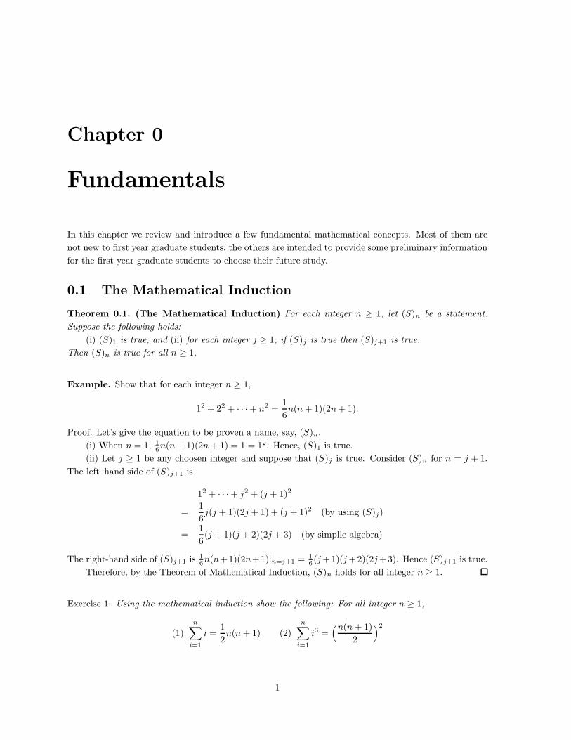
0.1 The Mathematical Induction

Theorem 0.1. (The Mathematical Induction) For each integer n ≥ 1, let (S)n be a statement.

Suppose the following holds:

(i) (S)1 is true, and (ii) for each integer j ≥ 1, if (S)j is true then (S)j+1 is true.

Then (S)n is true for all n ≥ 1.

Example. Show that for each integer n ≥ 1,

12 + 22 + · · · + n2 =1

6n(n + 1)(2n + 1).

Proof. Let’s give the equation to be proven a name, say, (S)n.

(i) When n = 1, 16n(n + 1)(2n + 1) = 1 = 12. Hence, (S)1 is true.

(ii) Let j ≥ 1 be any choosen integer and suppose that (S)j is true. Consider (S)n for n = j + 1.

The left–hand side of (S)j+1 is

12 + · · · + j2 + (j + 1)2

=1

6j(j + 1)(2j + 1) + (j + 1)2 (by using (S)j)

=1

6(j + 1)(j + 2)(2j + 3) (by simplle algebra)

The right-hand side of (S)j+1 is 16n(n+1)(2n+1)|n=j+1 = 1

6 (j +1)(j +2)(2j +3). Hence (S)j+1 is true.

Therefore, by the Theorem of Mathematical Induction, (S)n holds for all integer n ≥ 1.

Exercise 1. Using the mathematical induction show the following: For all integer n ≥ 1,

(1)

n∑

i=1

i =1

2n(n + 1) (2)

n∑

i=1

i3 =(n(n + 1)

2

)2

1

2 CHAPTER 0. FUNDAMENTALS

0.2 Sets

A set is a collection of things that have certain properties. It can be represented by a list, or

{x | properties of x} or {thing in category | properties of the thing}

If every element in a set A is also in a set B, then A is called a subset of B and B a supset of A,

written as A ⊂ B or B ⊃ A. The notation x ∈ A means that x is an element of A; similarly, x 6∈ A

means x is not in A.

One notices that A ⊂ A but A 6∈ A.

A set contains nothing is called an empty set, written as ∅.

For sets, we can define a few operations:

(i) Union: A ∪ B := {x | x ∈ A or x ∈ B};(ii) Intersection: A ∩ B := {x | x ∈ A and x ∈ B};(iii) Exclusion: A \ B := {x | x ∈ A, x 6∈ B};(iv) Product: A × B := {(a, b) | a ∈ A, b ∈ B};(v) power : S2 = S × S, AB = Πb∈BA.

Common Notations:

Z = all integers = {0,±1,±2, · · · }Q = all rational numbers = {p/q | p, q ∈ Z, q 6= 0}R = all real numbers

C = all complex numbers

Sn−1 = the unit sphere centered at the origin in Rn = {x ∈ Rn | |x| = 1}

Example. Let A = {0, 1}, B = {1, 2, 3, 4, · · · }. Then

A ∪ B = {0, 1, 2, · · · } = {n ∈ Z | n ≥ 0},A ∩ B = {1};A \ B = {0};

AB = Π∞i=1A = {(a1, a2, · · · ) | ai = 0 or 1 for all i ≥ 1}

There are two other ways to visualize the set AB .

(1) For any element (a1, a2, · · · ) ∈ AB , we relate it to a set consisting of those integer i for which

ai = 1. In such a manner, AB has a 1-1 correspondance to all subsets of B. Quite often, we use 2S to

denote all the subsets of S.

(2) If we use the binary system for all real numbers, any real number in [0, 1) can be written as

0.a1a2 · · · where ai is either 0 or 1. Hence, there is a 1-1 correspondance between all real numbers in

[0, 1) to AB . A sequence a1a2 · · · is called a binary sequence.

Exercise 2. Show that A ⊂ B ⇐⇒ A ∩ B = A.

Exercise 3. Let |A| denote the number of elements in A. With the convention that ∞ = ∞ show that for

any sets A and B,

|A ∩ B| + |A ∪ B| = |A| + |B|

0.3. MAPPING 3

0.3 Mapping

Let X and Y be two sets. A mapping, also called a map or a function, from X to Y is a rule that

assigns each element in X a value in Y . Y is called the image domain and X the definition domain. For

x ∈ X , its assigned value under a mapping f is denoted by f(x).

A mapping f from X to Y is written as f : X → Y or with more information, f : x ∈ X → f(x) ∈ Y .

A mapping is a rule. It can be regarded a machine. The entry can be regarded as an input, its

assigned value as the output.

x −→ f −→ f(x)

Definition 0.1. Let f : X → Y be a map.

(i) f is called injective (or one-to-one) if

∀x1, x2 ∈ X, x1 6= x2 =⇒ f(x1) 6= f(x2).

Alternatvely, f is injective if and only if f(x) = f(y) =⇒ x = y.

(ii) f is called surjective (or onto) if f(X) = Y ; in other words, for each y ∈ Y , there eixts x ∈ X

such that f(x) = y. (Here f(X) = {f(x) | x ∈ X}.)(iii) A function is called bijective (or a bijectin, or a one-to-one correspondence) if it is both

injective and surjective.

Definition 0.2. Let f : X → Y and g : Y → Z. The composition g ◦ f : X → Z is defined by

g ◦ f(x) = g(f(x)) ∀x ∈ X.

Consider the sine function. For an input x ∈ R, its output is sin x. Here we should make a clear

distinction between ”sin” and sinx; the former is a function and the later is a number.

On the other hand, notations are often abused for the purpose of convenience. The notation x2

could have two meanings: (i) the value x2, which is a default meaning, and (ii) the square function

: x ∈ C → x2 ∈ C. Whenever necessary, the second meaning needs to be specified.

Example. Let f : (u, t) ∈ U × [0,∞) → V be a function.

For each fixed t ≥ 0, we have a function f t : u ∈ U → f(u, t) ∈ V .

In addition, F : t ∈ [0,∞) → f t is also a function whose definition domain is [0,∞) and whose

image domain is the set W consisting of all functions from U to V .

To avoid the indexed notation f t, we use the notation f(·, t) to represent the function u → f(u, t),

where the · is called the dummy variable. The advantage of using f(·, t) instead of f(u, t) is that the

later could have many meanings.

Therefore, F : t ∈ [0,∞) → f(·, t) ∈ W defines a function. The definition domain of F is [0,∞),

the image domain is W , and the rule is F (t) = f(·, t).Similarly, f(u, ·) represents the function: t ∈ [0,∞) → f(u, t) ∈ Y . Also G : u ∈ U → f(u, ·) defines

a function with definition domain U and image domain Z being the set of function from [0,∞) to V .

Now suppose U = C2([0, 1] → R), the set of all twice differentiable functions from [0, 1] to R, and

V = C([0, 1]), the set of all continuous functions from [0, 1] to R. Define f(u, t) =√

t u + u′′ where u′′

represents the second order derivative of u. Then for any t ≥ 0, f(·, t) is a function, whose definition

domain U and image dimain V are spaces of functions.


Depending on the definition and image domains, more accurate names are used for mappings.

When the definition domain and the image domain are quite simple, e.g. points, a mapping is often

called a function.

When the image domain consists of numbers and the definition domain is not considered as very

simple, a mapping is often referred to as a functional.

When both the definition domain and the image donain are sets of functions, so the mapping maps

one function to another, the mapping is often called an operator. That is, an operator is a function of

functions.

Example. Let C([0, 1]) denote the set consisting of all functions that are continuous on [0, 1]. Set

X = C([0, 1]) and Y = R. We define a mapping L from X to Y by

L(f) :=

∫ 1

0

f(t)dt ∀f ∈ X.

Note that the definition domain X of L consists of functions, i.e., the entry of L are functions. Since

the image domain is the real line, L is a also called a functional. It mapps the “sine” function to the

real value 1 − cos 1, the “cosine” function to the real value sin 1, the “square” function to 1/3, and the

“cubic” function to 1/4.

An abused expression L(2x) = 1, however, should be correctly understood as L(f) = 1 where f is

the function defined as f : x ∈ [0, 1] → 2x.

Example. Let C1((0, 1)) be the set consisting of all functions that are differentiable in (0, 1). Set

X = C1((0, 1)) and Y = C((0, 1)) we define L from X to Y by

L(f) = f ′ ∀f ∈ X

where f ′ represents the derivative of f . In this setting, L is often called an operator, or a linear differential

operator.

In the same manner, the expression L(x2) = 2x should be understood correctly.

0.4. BINARY OPERATION 5

0.4 Binary Operation

Let S be a set.

A unitary operation on S is a mapping from S to S. For R, sin, cos, exp, log,√

are unitary operations.

It takes only one entry.

A binary operation on S is a mapping from S2 to S. For R, addition, subtraction, multiplication,

division are all binary operations. Each of them needs two entries.

Definition 0.3. Let ∗ : (a, b) ∈ S2 → a ∗ b ∈ S be a binary operation.

(i) ∗ is called associative if (a ∗ b) ∗ c = a ∗ (b ∗ c) ∀ a, b, c ∈ S.

(ii) ∗ is called commutative if a ∗ b = b ∗ a ∀ a, b ∈ S.

(iii) A left identity for ∗ is an element e ∈ S such that e ∗ a = a ∀ a ∈ S.

A right identity for ∗ is an element e ∈ S such that a ∗ e = a ∀ a ∈ S.

An identity for ∗ is an element e ∈ S such that a ∗ e = e ∗ a = a ∀ a ∈ S.

Suppose ∗ admits an identity e. If a ∗ b = b ∗ a = e, then b is called the inverse of a.

An indentity, if it exists, is unique. Similarly, an inverse, if it exists, is also unique.

When a set is equipped with certain operations, it becomes a structured set.

For an associative binary operation +, the expression a1 + a1 + a3 or

a1 + a2 + · · · + an

makes perfect sense, since the order of performing + is irrelavent.

Exercise 4. Let S = R2 = {(a, b) | a, b ∈ R} and define a binary operation “∗” for S by

(a, b) ∗ (c, d) := (ac, ad) ∀ (a, b), (c, d) ∈ S.

Show (i) ∗ is asociative; (ii) ∗ is not commutative; and (iii) there are infinitely many left identities.

Definition 0.4. Let (S1, ∗) and (S2, ·) be two sets with binary operations ∗ and ·. A mapping f : S1 → S2

is said to commute with or preserve the binary operation if

f(a ∗ b) = f(a) · f(b) ∀ a, b ∈ S1.

Example. Consider C. Fix a complex number a ∈ C. Assume that a 6= 0 and a 6= 1.

The map f : x ∈ C → f(x) = ax ∈ C preserves the addition of C since for every x, y ∈ C,

f(x + y) = a(x + y), f(x) + f(y) = ax + ay,

and by the law of distribution, a(x + y) = ax + ay.

On the other hand, the map does not preserve the multiplication since

f(xy) = axy, f(x)f(y) = axay = a2xy.

The map g : x ∈ C → g(x) = a + x ∈ C preserves neither the addition nor the multiplication since

g(x + y) = a + (x + y) = a + x + y, g(x) + g(y) = (a + x) + (a + y) = 2a + x + y;

g(xy) = a + xy, g(x)g(y) = (a + x)(a + y) = a + xy + a(x + y).

Definition 0.5. Let S be a set equipped with two binary oprations + and ∗. We say ∗ distributes on +

(or (+, ∗) satisfies the distribution law) if

a ∗ (b + c) = (a ∗ b) + (a ∗ c), (b + c) ∗ a = (b ∗ a) + (b ∗ c) ∀ a, b, c ∈ S.


0.5 Group

Definition 0.6. Let S be a set and ∗ be a binary operation. (S, ∗) is called a group if

(i) ∗ is associative, (ii) there is an identity, and (iii) every element in S admits an inverse.

A group is called commutative, or Abelian, if its binary operation is commutative.

Example. The following are commutative groups:

(Z, +), (Q \ {0},×), (C, +), (C \ {0},×).

Example. Let A be a set. Let S be the set that consists of all bijective functions from A to A. On S,

we define the binary operation “◦” as the composition of functions; more precisely, for f, g ∈ S, f ◦ g is

defined by

(f ◦ g)(x) = f(g(x)) ∀x ∈ A

Since the image domain of g is A and the definition domain of f is also A, f ◦ g is a function from A to

A. It is easy to show that f ◦ g : A → A is bijective. Hence f ◦ g ∈ S. One can show that (S, ◦) is a

group, called the permutation group of A.

Now suppose A = {1, 2, · · · , n}. A bijective mapping from A to A is called a permutation of n

objects. A permutation p can be recorded as

(1 2 · · · n

p(1) p(2) · · · p(n)

)

or simply (p(1) p(2) · · · p(n))

There are a total of nn number of functions from A to A. Among them, only n! of them are 1 − 1.

Hence, a permutation group of n objects has a total of n! elements.

Definition 0.7. Let (G, ∗) be a group and a ∈ G. The (left) action of a on G is a mapping T a : G → G

defined by

T a(x) = a ∗ x ∀x ∈ G.

All actions of a group, under the binary operation defined as the composition of mapping, form

a group call the group of action. The group of action is identical, modulo an isomprphism, to the

original group. Namely, the mapping a → T a is a 1-1 correspondance and preserves the multiplcation:

a ∗ b → T a∗b = T a ◦ T b.

Although a group is isomprphic to its action group, sometimes the study of later is easier than that

of the former.

Exercise 5. Consider the magic cube which has six faces and each face is covered by 9 identical square

tiles.

Provide an identification that associates the transformation of the magic cube to the permutation

group of 54 objects.

Also discuss the action group.

0.6. RING AND FIELD 7

0.6 Ring and Field

Definition 0.8. Let S be a set and + and ∗ are two binary operations on S.

(i) (S, +, ∗) is called a ring if (S, +) is a commutative group, ∗ is associative, and there holds the

laws of distribution

a ∗ (b + c) = (a ∗ b) + (a ∗ c), (a + b) ∗ c = (a ∗ c) + (b ∗ c) ∀a, b, c ∈ S.

(ii) (S, +, ∗) is called a field if (S, +, ∗) is a ring and (S \ {0}, ∗) is a commutative group, where 0

is the identity for the + operation.

The extra property needed for a commutative ring to become a field is the binary operation of

division (multiplication of the inverse). We use −a to denote the inverse of a under addition, and a−1

the inverse of a under multiplication. Also, 0 is the identity for addition, 1 the identity for multiplication,

and −1 the inverse of 1 under addition. Note that −a = (−1)a = a(−1)

Example. (Z, +,×) is a commutative ring, but not a field, whereas (Q, +,×) is a field.

Example. For every f, g ∈ C([0, 1]), we define f + g and fg by

(f + g)(x) = f(x) + g(x), (fg)(x) = f(x)g(x) ∀x ∈ [0, 1].

Then f + g, fg ∈ C([0, 1]). With such defined addition and multiplication, C([0, 1]) is a commutative

ring, but not a field.

Example. For a positive integer p and any integer q, let q mod (p) denote the remainder of q divided

by p, where the remainder lies between 0 and p − 1.

Let p be a prime number and set Zp = {0, 1, · · · , p− 1}. On Zp we define addition + and multipli-

cation × by

i+j = (i + j) mod (p), i×j = ij mod (p)

Then (Zp, +,×) is a field, having p elements.

Exercise 6. Show that Zp, under the mod (p) calculation, is a field if p is a prime number.

Exercise 7. Let S = {a + b√

5 | a, b ∈ Q} and U = {a + b√

5 + c√

7 + d√

35 | a, b, c, d ∈ Q}. Define

the addition “+”and multiplication “×” as that for real numbers. Show that (U, +,×) is a subfield of

(R, +,×), and (S, +,×) is a subfield of (U, +,×).


0.7 The Fundamental Theorem of Algebra

Let F be a field. We can introduce a polynomial of degree n:

P (x) = a0xn + a1x

n−1 + · · · + an−1x + an

where x ∈ F is a variable, a0, a1, · · · , an are given coefficients in F and a0 6= 0.

Similarly, one can form polynomials of multiple variables x = (x1, · · · , xm) ∈ Fm:

P (x) =∑

|α|≤n

aαxα

where

α = (α1, · · · , αm), αi a non-negative integer,

|α| = α1 + · · · + αm

xα = xα1

1 · · ·xαm

m

An algebraic equation is an equation of the form P (x) = 0 where P is a polynomial of x. For a

single variable, an algebraic equation of degree n can be written as

xn + a1xn−1 + · · · + an−1x + an = 0.

By using long-division, we have

Lemma 0.1. Let P (x) = xn + a1xn−1 + · · ·+ an be a polynomial of degree n. Suppose P (r) = 0. Then

there is a polynomial Q of degree n − 1 such that

P (x) = (x − r)Q(x).

We remark that the result is true only if the underlying set for coefficients is a field.

Theorem 0.2. (Theorem of Common Divisior) Let P and Q be polynomials and R = (P, Q) the

common divisor of P and Q. Then there exist polynomials f and g such that

f(x)P (x) + g(x)Q(x) = R(x).

As a consequence, if two polynomials P and Q are prime to each other, i.e., (P, Q) = 1, then there

exist polynomials f and g such that

f(x)P (x) + g(x)Q(x) = 1.

Exercise 8. Prove the Theorem of Common Divisor.

It is easy to see that not every algebraic equation is solvable if F = Q or R. However, for C, we

have the following theorem:

Theorem 0.3. (The Fundamental Theorem of Algebra) Let C be the set of complex numbers.

For every a1, · · · , an ∈ C, there exist r1, · · · , rn ∈ C such that

P (z) := zn + a1zn−1 + · · · + an−1z + an = (z − r1)(z − r2) · · · (z − rn).

Consequently, the algebraic equation

zn + a1zn−1 + · · · + an−1z + an = 0

has exactly n roots (counting multiplicity) in C.

0.7. THE FUNDAMENTAL THEOREM OF ALGEBRA 9

Proof. We need only consider the case n ≥ 2. It suffcies to show that P (z) = 0 has a root in C.

Setp 1. We show that there exists r ∈ C such that |P (r)| ≤ |P (z)| for all z ∈ C.

Let R = 1 + |a1| + · · · + |an|. When |z| ≥ R, we see that

|P (z)| = |zn−1(z + a1 + · · · + an/zn−1)| ≥ Rn−1(R − |a1| − · · · − |an|) ≥ Rn−1 ≥ R.

Since |P (·)| is continuous on BR := {z ∈ C||z| ≤ R} and BR is bounded and closed, there exists a point

r ∈ BR such that |P (r)| ≤ |P (z)| for all z ∈ BR. As |P (r)| ≤ |P (0)| = |an| ≤ R − 1, we see that

|P (r)| ≤ |P (z)| for all z ∈ C.

Setp 2. We show that |P (r)| = 0 by using a contradiction argument. Suppose, on the contrary, that

|P (r)| > 0. Note that, for any y ∈ C,

P (r + y) = (r + y)n + a1(r + y)n−1 + · · · + an = P (r) + b1y + · · · + bn−1yn−1 + yn

where b1, · · · , bn−1 are complex numbers depending only on a1, · · · , an−1, and r. We write bn = 1.

Let j ∈ {1, · · · , n} be the minimum integer such that bj 6= 0. Then, when |y| < 1,

|P (r + y)| = |P (r) + bjyj + · · · + bnyn|

≤ |P (r) + bjyj | + |y|j+1M, M :=

n∑

i=j+1

|bi|(= 0 if j = n.)

Now let c be one of the jth roots to −P (r)/bj , i.e., cj = −P (r)/bj . Set y = εc where ε is a real

number satisfying 0 < ε < 1/(1 + |c|). Then |y| < 1, yj = −εjP (r)/bj , and ε < 1. Consequently,

|P (r + y)| ≤ |P (r) − εjP (r)| + εj+1|c|j+1M

= |P (r)|{1 − εj + εj+1|c|j+1M/|P (r)|} < |P (r)|

for all sufficiently small positive ε. But this contradicts the mimimality of |P (r)|. This contradiction

shows that P (r) = 0, thereby completing the proof.

In this proof, we used two non-trivial facts:

(i) A continuous function attains its minimum over a bounded closed set.

(ii) For any complex number a and any positive interger j, there exixts at least a complex number

c such that cj = a.

In the theory of algebra, the following language is used.

Definition 0.9. A field is called closed if every polynomial can be factorized into linear factors.

The fundamental Theorem of Algebra: The field of complex number is closed.

Exercise 9. Let f be a continuous function defined on [0, 1]. Show that there exists a ∈ [0, 1] such that

f(a) ≤ f(x) for all x ∈ [0, 1].

Exercise 10. Show that for every complex number a 6= 0 and integer n ≥ 1, the equation zn = a has at

least one root.


0.8 Vector Space

In the sequel, F is a field whose addition is denoted by a + b and multiplcation by ab for any a, b ∈ F.

The identity of the addition is denoted by 0 and the identity of multiplication by 1. An element in F

will be referred to as a number or a scalar.

Definition 0.10. Let (V, +) be an commutative group and F be a field. V is called a vector space

over F if a scalar muliplition : (a,x) ∈ F × V → ax ∈ V is so defined that it satisfies the following

1x = x, a(bx) = (ab)x, a(x + y) = (ax) + (ay), (a + b)x = (ax) + (bx) ∀ a, b ∈ F,x,y ∈ V.

When the field F is replaced by a ring R, the corresponding V is called an R-module.

There are two additions here: the addition of vectors and the addition of numbers. The identity of

the vector addition will be denoted by 0.

There are also two “multiplications” here: the multiplication of numbers and the scalar mutiplication

between numbers and vectors. One notices that multiplcation between vectors is not defined.

Definition 0.11. A vector space V over a feld F is called an algebra if V is supplemented with an

multiplication ∗ : V 2 → V such that ∗ is associative and satisfies

a(x ∗ y) = (ax) ∗ (y) = x ∗ (ay) ∀ a ∈ F,x,y ∈ V.

In the sequel, a vector space means a vector space over a field F.

In the previous definition of vector spaces, scalars are multiplied from the left to vectors. Hence,

the vector space is indeed a left vector space. Similarly, we have right vector spaces. Throughout this

course, we avoid this distinction by using the convention

xa := ax ∀a ∈ F, x ∈ V.

Also we use the convention that scalar multiplication proceeds the addition operation. In this

manner, the following expression is well–defined:

n∑

i=1

aixi = a1x1 + · · · + anxn

Exercise 11. Let V be a vector space. Show that 0x = 0 and a0 = 0 for all a ∈ F and x ∈ V . Also show

that ax = 0 if and only if either a = 0 or x = 0.

Definition 0.12. Let X and Y be subsets of a vector space V (over a field F).

(i) X is called a subspace of V if X itself is a vector space (with the same addition and scalar

multiplication as that for V );

(ii) X ∪ Y := {z | z ∈ X or z ∈ Y };(iii) X + Y := {x + y | x ∈ X,y ∈ Y };(iv) X ∩ Y := {z | z ∈ X and z ∈ Y }.

Lemma 0.2. Let X be a subset of a vectoe space V over a field F. X is a subspace if and only if

ax + y ∈ X ∀x,y ∈ X, a ∈ F.

0.8. VECTOR SPACE 11

Lemma 0.3. If X and Y are subspaces, so are X + Y and X ∩ Y .

Exercise 12. Prove Lemmas 0.2 and 0.3.

Exercise 13. Let X and Y be subspaces of V . Show X ∪ Y is a subspace if and only if either X ⊂ Y or

Y ⊂ X.


0.9 Relations and Quotients

Definition 0.13. Let S be a set.

(1) Let R ⊂ S2 := S × S. Then a relation ∼ induced by R is defined by

x ∼ y ⇐⇒ (x, y) ∈ R.

(2) A relation ∼ is called

(i) symetric if x ∼ y ⇒ y ∼ x;

(ii) reflective if x ∼ x for all x ∈ S;

(iii) transitive if x ∼ y, y ∼ z ⇒ x ∼ z;

(3) A relation is called an equivalence relation if it is symmetric, reflective, and transitive.

(4) Given an equivalence relation ∼, the congruence class containing x ∈ S is the set

{x} := {z ∈ S | z ∼ x}.

and the set of congruence classes is defined as

G/ ∼:= {{x} | x ∈ G}.

(5) Let ∗ be a binary operation for S. An equivalence relation ∼ is called preserving the operation if

x1 ∼ x2, y1 ∼ y2 =⇒ x1 ∗ y1 ∼ x2 ∗ y2.

Example. Let S = R.

(1) Define x ∼ y if x < y. This relation is transitive, but neither symmetric nor reflective.

(2) Define x ∼ y if x ≤ y. This relation is transitive and reflective, but not symetric.

(3) Define x ∼ y if x − y ∈ Q. This is an equivalence relation, and {x} = x + Q defined as

x + Q := {x + y | y ∈ Q}

Theorem 0.4. (1) Let (G, ·) be a group and ∼ be an equivalence relation for G that preserves the binary

operation ·. Define a binary operation ∗ for G/ ∼ by

{a} ∗ {b} := {a · b} ∀a, b ∈ G

Then (G/ ∼, ∗) is also group.

(2) Let (F, +, ∗) be a field and ∼ be an equivalence relation on F that preserves +and ∗. Define

{a}+ {b} := {a + b}, {a} ∗ {b} := {a ∗ b} ∀a, b ∈ F.

Then (F/ ∼, +, ∗) is also a field.

(3) Let (V, +) be a vector space over a field F and ∼ be an equivalence relation on V that preserves

the vector addition and scalar multiplication, i.e,

x1 ∼ x2,y1 ∼ y2 =⇒ x1 + y1 ∼ x1 + y2, ax1 ∼ ax2∀a ∈ F

Then V/ ∼ is also a vector space if the vector addition and scalar multipliction are defined by

{x} + {y} := {x + y}, a{x} := {ax} ∀x,y ∈ V, a ∈ F.

0.9. RELATIONS AND QUOTIENTS 13

Proof. We only prove (1). First we show that ∗ is well–defined for G/ ∼; i.e., the definition is

independent the choices of a and b.

Let a, b ∈ G be arbitrary. Suppose a1 ∼ a and b1 ∼ b. Then as ∼ preserve the operation ·,a1 · b1 ∼ a · b so that {a1 · b1} = {a · b}. Hence, ∗ is well–defined.

Since (G, ·) is a group, for any {a}, {b}, {c} ∈ G/ ∼,

({a} ∗ {b}) ∗ {c} = {a · b} ∗ {c} = {(a · b) · c} = {a · (b · c)} = {a} ∗ {b · c} = {a} ∗ ({b} ∗ {c}).

{a} ∗ {e} = {a · e} = {a} = {e · a} = {e} ∗ {a}{a} ∗ {a−1} = {a · a−1} = {e}.

Hence, G/ ∼ is a group, with identity being {e} and the inverse of {a} being {a−1}.

Exercise 14. Prove (2) and (3) of the Theorem 0.4.

Exercise 15. Provide an example of a group (G, ·) and an equivalence relation ∼ which does not proserve

the multiplation of G. What would be the consequence if we try to define {a} ∗ {b} = {a · b} on G/ ∼.

Definition 0.14. (1) Let (G, ∗) be a group and H be a subgroup of G. Two elements a, b ∈ G are called

congruent modulo H, denoted by a ≡ b mod (H), if ab−1 ∈ H. (Here b−1 denote the inverse of b under

∗. )

(2) Let V be a vector space and H be a subspace. Two vectors x and y are called congruent modulo

H, denoted by x ≡ y mod (H), if x− y ∈ H.

Theorem 0.5. (1) Let (G, ∗) be a group, H be a subgroup of G, and ≡ be the congruent modulo H

relation. Assume in addition that H is a normal subgroup, i.e., aHa−1 = H for all a ∈ G. Then the set

G/ ≡, with the induced operation

{x} ∗ {y} := {x ∗ y}is a group, denoted by G/H and called the quotient group of G modulo H.

(2) Let V be a vector space over a field F, H be a subspace V , and ≡ be the congruent modulo H

relation. Then the set V/ ≡, with the induced vector addition and scalar multiplication

{x}+ {y} := {x + y}, a{x} := {ax}

is a vector space over F, denoted by V/H and called the quotient space V modulo H.

Proof. We only prove (1), leaving the proof of (2) as an exercise.

First we show that ≡ is an equivalence relation.

(i) Suppose x ≡ y. Then xy−1 ∈ H . As H is a group, (xy−1)−1 = yx−1 ∈ H , so that y ≡ x.

(ii) As xx−1 = e ∈ H , x ≡ x.

(iii) Suppose x ≡ y and y ≡ z. Then xy−1 ∈ H and yz−1 ∈ H . Consequently, xz−1 =

(zy−1)(yz−1) ∈ H so x ≡ z. Hence, ≡ is an equivalence relation.

Next we show that ≡ preserve the multiplication structure. Suppose x1 ≡ y1 and x2 ≡ y2. Then

x1y−11 ∈ H and x2y

−12 ∈ H . Consequently, (x1x2)(y1y2)

−1 = x1x2y−12 y−1

1 = x1(x2y−12 )y−1

1 (x1y−11 )y1x

−11 ∈

x1Hy−11 Hy1x

−11 = x1HHx−1

1 = x1Hx−11 = H . Hence, x1x2 ≡ y1y2. By the previous theorem, G/ ≡ is

a group.

Exercise 16. Let (G, ∗) be a finite group and H be a subgroup. Denote by |G| the number of elements

in G. Show that |G|/|H | is an integer. In particular, if G is commutative or H is normal, then

|G/H | = |G|/|H |.Exercise 17. Prove the second assertion of Theorem 0.5


0.10 Banach and Hilbert Spaces

Binary operations are structures mainly used in algebra. Here we introduce some structures used in

analysis.

Definition 0.15. (1) Let S be a set. A function d : S2 → R is called a distance function if

(i) d(x, x) = 0 for all x ∈ S;

(ii) d(x, y) = d(y, x) > 0 for all x 6= y;

(iii) d(x, z) ≤ d(x, y) + d(y, z) for all x, y, z ∈ S.

(2) Let S be a set equipped with a distance. A sequence {xi}∞i=1 is called a Cauchy sequence if

limi,j→∞

d(xi, xj) = 0

The set S is called complete if every Cauchy sequence has a limit in S; namely, if {xi}∞i=1 is a

Cauchy sequence in (S, d), then there exists x ∈ S such that

limi→∞

d(xi, x) = 0.

When the underlying set S is a vector space over the field R or C, we ofter require the distance

scale with the scaler multiple and the triangle inequality be compatible with the vector addition. This

leads to a metric space.

Definition 0.16. Let V be a vector space over F = R (or C). A norm on V is a mapping ‖ · ‖ : x ∈V → ‖x‖ ∈ [0,∞) that has the following properties:

(i) ‖x‖ = 0 if and only if x = 0;

(ii) ‖x + y‖ ≤ ‖x‖ + ‖y‖ for all x,y ∈ V ;

(iii) ‖ax‖ = |a|‖x‖ for all a ∈ F and x ∈ V .

A normed vector space (V, ‖ · ‖) equipped with the distance

d(x,y) := ‖x− y‖

is called a metric (vector) space.

Definition 0.17. A Banach Space is a complete normed vector space (over R or C).

Theorem 0.6. Any normed vector space over R or C can be completed to become a Banach space.

In the history of mathematics, the completion (fill in “gaps”) from the rational number field Q

to the real number field R took thousands of years, and is considered as one of the most important

development of mathematics. The stated theorem follows this line of development.

Proof. Let (V, | · |) be a normed vector space over R. Then Cauchy sequences are well–defined. We

let U be the collection of all Cauchy sequences. We define a relation ∼ on U by

{ξj}∞j=1 ∼ {ηj}∞j=1 if limj→∞

|ξj − ηj | = 0.

It is easy to see that ∼ is an equivalence relation. In a ddition,

limj→∞

|ξj | = limj→∞

|ηj | if {ξj}∞j=1 ∼ {ηj}∞j=1

Set V = U/ ∼. Define, for an arbitrary element{

{ξj}∞j=1

}

∈ V ,

∥∥∥

{

{ξj}∞j=1

}∥∥∥ = lim

j→∞|ξj |.

0.10. BANACH AND HILBERT SPACES 15

This is well–defined since the right–hand side does not depend on the choice of the Cauchy sequence

in {{ξj}∞j=1}. We define {{ξj}} + {{ηj}} = {{ξj + ηj}} and a{{ξj}} = {{aξj}} for all a ∈ R and

{{ξj}}, {{ηj}} ∈ V .

One can also show that (V , ‖ · ‖) is a normed vector space over R (We leave the details to the

readers), with zero defined by {{0}∞j=1}, the class of all sequences that approach 0.

We now show that V is complete. Suppose {uk}∞k=1 is a Cauchy sequence in V , i.e., writing

uk = {{ξkj }∞j=1}, there holds

0 = limk,l→∞

‖uk − ul‖ = 0 where ‖uk − ul‖ = limj→∞

|ξkj − ξl

j |.

Since for each fixed k, {ξkj }∞j=1 is a Cauchy sequence, there is J(k) ≥ k such that |ξk

j − ξki | ≤ 1/k

for all i, j ≥ J(k).

We now define ηn = ξnJ(n) for n ≥ 1 and consider the sequence {ηn}∞n=1. For all k, l ≥ 1,

|ηk − ηl| = |ξkJ(k) − ξl

J(l)| ≤ lim supj→∞

(

|ξkJ(k) − ξk

j | + |ξkj − ξl

j | + |ξlj − ξl

J(l)|)

≤ 1/k + ‖uk − ul‖ + 1/l

Sending k, l → ∞ we see that {ηn}∞n=1 is a Cauchy sequence. Hence u := {{ηn}∞n=1} ∈ V . In addition,

liml→∞

‖u− ul‖ = liml→∞

limn→∞

|ηn − ξln| = lim

l→∞lim

n→∞|ξn

J(n) − ξln|

≤ liml→∞

limn→∞

lim supj→∞

(

|ξnJ(n) − ξn

j | + |ξnj − ξl

j | + |ξlj − ξl

n|)

≤ limn,l→∞

(

1/n + ‖un − ul‖)

+ liml→∞

limn,j→∞

|ξlj − ξl

n| = 0

Thus, u ∈ V is the limit of the Cauchy sequence {uk}∞k=1. This shows that V is complete.

Finally, V can be regarded as a subset of V if we identify each element x ∈ V to x := {{x}∞j=1} in

V . In addition, |x| = ‖x‖ for all x ∈ V . Hence, V is a completion of V . In addition V is dense in V

(The proof is left as an exercise).

Definition 0.18. An inner product for a vector space V over R or C is a mapping (·, ·) : (x,y) ∈ V 2 → R

or C such that

(i) (·, ·) is (complex) symmetric and bilinear,i.e.

(x,y) = (y,x), (ax + by, z) = a(x, z) + b(y, z), ∀x,y, z ∈ V, a, b ∈ R or C;

(ii) (x,x) > 0 for all x 6= 0.

Lemma 0.4. Let V be a vector space over R or C and with an inner product (·, ·). Then the following

defined

‖x‖ :=√

(x,x) ∀x ∈ V

is a norm, and is called the induced norm by the inner product.

Exercise 18. Prove Lemma 0.4.

Definition 0.19. A Hilbert space is a vector space over R or C equipped with an inner product with

the property that the space is complete with the induced norm (i.e., a Banach space).


Hence, a Hilbert space is a Banach space (V, ‖ · ‖) equipped with an inner product (·, ·) that is

compatible with the norm: ‖x‖2 = (x,x) for all x ∈ V .

Theorem 0.7. Any vector space over R or (C) equipped with an inner product can be completed to

become a Hilbert space.

Exercise 19. Using Theorem 0.6 prove Theorem 0.7.

Example. The Euclidean space Rn is a Hilbert space.

0.11. TOPOLOGICAL SPACE 17

0.11 Topological Space

Definition 0.20. (1) Let S be a set and O be a certain collection of subsets of S. We say that O defines

a topology for S if

(i) ∅ ∈ O, S ∈ O;

(ii) If U1, U2 ∈ O then U1 ∩ U2 ∈ O;

(iii) The union of arbitrary number of sets in O is still in O; i.e., for arbitrary index set I, if Ui ∈ Ofor all i ∈ I, then ∪i∈IUi ∈ O.

(2) For a topological space (S,O), a subset of S is called open if it is an element of O; a subset D

of S is called closed if its complement Dc := {x ∈ S | x 6∈ D} is an open set.

Example. Let S = R. A set O in R is called open if for every x ∈ S, there exists δ > 0 such that

(x − δ, x + δ) ⊂ O.

Let O the collection of all open sets of R. Then (R,O) is a topological space.

Theorem 0.8. Let S be a set and A be a collection of certain subsets of S (i.e a subset of 2S). Then

there exists a unique topological space (S,O) such that

(i) A ⊂ O;

(ii) If (S, O) is a topology space such that A ⊂ O, then O ⊂ O.

In Rn, distance is defined, and a compact set can be defined as a bounded closed set. For a

topological space where distance maynot be defined, a compact is defined as follows.

Definition 0.21. Let {S,O} be a topological space and A be a subset.

(i) A collection of sets {Oi}i∈I is called an open covering if Oi ∈ O for all i ∈ I and A ⊂ ∪i∈IOi.

(ii) A set is called compact if any open covering contains a finite subcovering, ( i.e. finitely many

open sets whose union cover the set).

(iii) A set is called precompact if its closure (the smallest supset that are closed) is compact.

Exercise 20. Show that in R, a set is compact if and only if it is closed and bounded. Consequently, a

set is precompact if and only if it is bounded.


0.12 Morphsims

Given a space (i.e. set) with a structure (algebric, analytic, or topologic), the name, or representation,

of each element in the space is irrelavant to the structure. A mathematical way of identifying all spaces

with the same structure is using isomorphism.

Definition 0.22. (1) Let (G1, ∗) and (G2, ·) be two groups. A mapping f : G1 → G2 is called an

homomorphism if it preserves the group structure, i.e.

f(a ∗ b) = f(a) · f(b) ∀ a, b ∈ G1.

Thst is, the image of the multiple is the multiple of the images.

(2) Let F1 and F2 be two fields. A mapping f : F1 → F2 is called a homomorphism if preserves the

field structure, i.e.

f(a + b) = f(a) + f(b), f(ab) = f(a)f(b) ∀a, b ∈ F1.

That is, the image of the sum or multiple is the sum or multiple of the images.

(3) Let V1 and V2 be two vector spaces over the same field F. A mapping f : V1 → V2 is called a

homomorphism if it preserves the vector space structure:

f(x + y) = f(x) + f(y), f(ax) = af(x) ∀a ∈ F,x,y ∈ V1.

That is, the image of the vector sum is the vector sume of the images, and the image of scalar multiple

is the scalar multiple of the image.

Hence, a homomorphism of group is a map commuting with the group multiplication. A homo-

morphism of field is a map that commutes with the field multiplication and addition. A homorphism of

vector space is a map that commutes with the vector addition and scalar multiplication.

Definition 0.23. A homomorphism X → Y is called

(i) monomorphism or an embedding if it is injective,

(ii) epimorphism if it is surjective,

(iii) isomorphism if it is bijetive,

(iv) endomorphism if X = Y (including the structures),

(v) automorphism if it is an isomorphism and X = Y (inclding the structures).

Two spaces are called isomorphic if there is an isomorphism.

Exercise 21. Define isomorphism for Banach spaces, Hilbet Spaces, and Topological spaces.

Exercise 22. Let F be a field. Let S = {1, 2, · · · , n}. Let V be the collection of all functions from S to

F. For f, g ∈ V and a ∈ F, we define functions f + g and af by

(f + g)(x) = f(x) + g(x), (af)(x) = af(x) ∀x ∈ S.

Then f + g ∈ V and af ∈ V . With such defined addition of elements in V and the scalar multiplication

between F and V , show that V is a vector space that is isomorphic to Fn.

Exercise 23. In what sense can one say that Cn is isomorphic to R2n?

Theorem 0.9. All automorphism of a space G, together with multiplication defined as the composition

of mappings, form a group.

0.12. MORPHSIMS 19

For vector spaces, all homomorphism form a vector space itself.

Theorem 0.10. Let U and V be vector spaces over the same field F. Then, Hom(U, V ), the set of all

homomorphisms from U to V , is a vector space over F if the vector addition f+g and scalar multiplication

af for f, g ∈ Hom(U, V ) and a ∈ F are defined by

(f + g)(x) = f(x) + g(x), (af)(x) = af(x) ∀x ∈ U.

Theorem 0.11. Let U be a vector space. Then Hom(U, U) is an algebra.

Exercise 24. Prove Theorems 0.9, 0.10, and 0.11.


0.13 Matrix Algebra

Linear mappings from Rn to Rm can be characterized by matrices. Consequently, the algebra of linear

mapping carries over to matrices.

Let A : Rn → Rm be a map that is linear, i.e.

A(ax + by) = aA(x) + bA(y) ∀ a, b ∈ R,x,y ∈ Rn.

From the definition of vector spaces and homomorphism of vector spaces, a mapping is a homomorphism

if and only if it is linear. We denote all the homomorphsm (linear mapping) by Hom(Rn, Rm).

A linear mapping can be characterised by nm real numbers. Indeed, let {e1, · · · , en} be the canonical

basis for Rm (i.e., ei has the ith component 1, all other 0), and {e′1, · · · , e′m} the canonical basis for Rn.

For each j = 1, · · · , n, A(e′j) ∈ Rm can be written as

A(e′j) = a1je1 + · · · + am

j em =

m∑

i=1

aijei, j = 1, · · · , m (0.1)

It is conventional an traditional to arrange the coefficients aij in a rectangle array

A = (aij)m×n :=

a11 · · · a1

n

.... . .

...am1 · · · am

n

. (0.2)

Such an array is called an m by n matrix, m being the number of rows, and n the number of columns.

We shall use a short notation (aij)m×n to denote the m × n matrix whose entry at the ith row and jth

column is aij for i = 1, · · · , m, j = 1, · · ·n.

Unlike the traditional notation where aij is used, here we use a tensor like notation aij , the superindex

i is the position in rows, and the subscript j the position in columns.

The jth column vector aj and the ith row vector ai can be written as

aj =

a1j

...am

j

, ai = (ai

1 · · · ain).

For each x ∈ Rn, writing x = x1e′1 + · · · + xne′n we then have, by the lienarity of A,

A(x) =

n∑

j=1

xjA(e′j) =

n∑

j=1

xj

m∑

i=1

aijei =

m∑

i=1

eiyi, yi :=

n∑

j=1

aijx

j

Hence, A is uniquely determined by the matrix A. It is easy to show that given an m by n matrix A,

the last quantity in the preceding equation defines a linear mapping from Rn to Rm. Hence, there is a

one-to-one correspondence betweem Hom(Rn, Rm) and all real m × n matrices.

Since Hom(Rn, Rm) is a vector space, it is natural to carry this structure (addition and scalar

multiplication) to matrices. This leads to the following definition:

Definition 0.24. Let F be a field (or a ring). Let α ∈ F and A = (aij)m×n and B = (bi

j)m×n be two

matrices whose enteries aij , b

ij are ∈ F. The matrix addition A + B and scalar multiplication αA is

defined by

A + B = (aij + bi

j)m×n, αA = (αaij)m×n.

0.13. MATRIX ALGEBRA 21

The (commonly used) matrix multiplication is induced from the composition of linear mappings.

Consider two linear mappings: B : Rp → Rn and A : Rn → Rm with its associated matrices

A = (aij)m×n and B = (bj

k)n×p, under the bases (e1, · · · , ep) for Rp, (e′1, · · · , e′n) for Rn and (e1, · · · , em)

for Rm. For mappings, the compositipn A ◦ B : Rp → Rm is defined by A ◦ B(x) = A(B(x)). Using

A(e′j) =∑m

i=1 aijei, B(ek) =

∑n

j=1 bjke

′j , and the linearity of the mappings, for each k = 1, · · · , p,

A ◦B(ek) = A(B(ek)) = A(

n∑

j=1

bjke

′j) =

n∑

j=1

bjkA(e′j)

=n∑

j=1

bjk

m∑

i=1

aijei =

m∑

i=1

( n∑

j=1

aijb

jk

)

ei =m∑

i=1

cikei, ci

k :=n∑

j=1

aijb

jk.

Thus, the mapping A◦B : Rp → Rm corresponds to the matrix C = (cik)m×p. This leads to the following

definition of the multiplication of matrices.

Definition 0.25. Let A = (aij)m×n be an m by n matrix and B = (bj

k)n×p be an n by p matrix with

enteries aij , b

jk ∈ F, a field or a ring. Then AB = (ci

k)m×p is an m by p matrix whose entry cik at the ith

row and kth column is defined by

cik =

n∑

j=1

aijb

jk, i = 1, · · · , m, k = 1, · · · , p.

Theorem 0.12. Let F be a field and m, n be positive integers. Then Mm,n(F), the set of all m × n

matrices with enteries in F form a vector space under componentwise addtion and scalar multiplication

in the Definition 0.24.

Theorem 0.13. Let F be a field and n be a posiive integer. Then Mn(F) = Mn,n(F) is an algebra,

under the matrix operations defined in Definitions 0.24 and 0.25.

The study of matrices is equivalent to the study of linear mappings, if one concerns only with the

matrix addition, scalar and matrix multiplication, as defined.

In the sequel, we shall identify a 1×1 matrix as a number; i.e. (a) = a. Also, we call a m×1 matrix

a row vctor and a 1 × p matrix a column vector. Also we use AT to denote its transpose, defined by

for A = (aij)m×n, AT = (bj

i )n×m, bji := ai

j .

In the spacial case where matrices are vectors, we have,

for x = (x1, · · · , xn), y =

y1

...yn

xy = (x1 · · ·xn)

y1

...yn

= x1y1 + · · ·xnyn = 〈x,y〉,

yx =

y1

...yn

(x1 · · ·xn) = (yi)n×1(xj)1×n = (yixj)n×n =

y1x1 · · · y1xn

.... . .

...ynx1 · · · ynxn

.


Also if for each j = 1, · · ·n, uj = (u1j · · ·um

j )T is a column vector, then

y1u1 + · · · + ynun = Uy, U := (u1 · · ·un) =

u11 · · · u1n

.... . .

...um1 · · · umn

, y :=

y1

...yn

.

The mapping in (0.1) can be written as

A(e′j) = (e1 · · ·em)aj , aj = a·j =

a1j

...am

j

,

A(e′1 · · · e′n) := (A(e′1) · · · A(e′n)) = (e1 · · · em)A, A = (aij)m×n.

0.14. HOMEWORK 23

0.14 Homework

1. Use the mathematical induction show the following:

(1)

n∑

i=1

i =1

2n(n + 1) (2)

n∑

i=1

i3 =(n(n + 1)

2

)2

2. Show that A ⊂ B ⇐⇒ A ∩ B = A.

3. Let S = R2 = {(a, b) | a, b ∈ R} and define a binary operation “∗” for S by

(a, b) ∗ (c, d) := (ac, ad) ∀ (a, b), (c, d) ∈ S.

Show that (i) “*” is asociative; (ii) “*” is not commutative; and (iii) there are infinitely many left

identities.

4. Show that if an associative binary operation admits a left identity and a right identity, then it

admits a unique identity.

5. Display the summation and multiplication tables for Z3, and show that it is a field.

6. Let S = {a + b√

5 | a, b ∈ Q} and U = {a + b√

5 + c√

7 + d√

35 | a, b, c, d ∈ Q}. Define the addition

“+”and multiplication “×” as that for real numbers. Show that (U, +,×) is a subfield of (R, +,×),

and (S, +,×) is a subfield of (U, +,×).

7. Let V be a vector space over F. Show that 0x = 0 and a0 = 0 for all a ∈ F and x ∈ V . Also show

that ax = 0 if and onlt if a = 0 or x = 0.

8. Let X and Y be subspaces of V . Show the following:

(i) X + Y is a subspace;

(ii) X ∩ Y is a subspace;

(iii) X ∪ Y is a subspace if and only if either X ⊂ Y or Y ⊂ X .

9. Let X be a subset of a vector space V . Show that X is a subspace if and only if ax + y ∈ X for

all x,y ∈ X and a ∈ F.

10. Discuss the possible extension for quotient fields.

11. Let (G, ∗) be a finite group and H be a subgroup. Denote by |G| the number of elements in G.

Show that |G|/|H | is an integer. In particular, if G is commutative, then |G/H | = |G|/|H |.

12. Let f be a mapping between two vector spaces V1, V2 over the same field F . Show that the

properties

f(x + y) = f(x) + f(y), f(ax) = af(x) ∀a ∈ F,x,y ∈ V1

is equivalent to the property

f(ax + y) = af(x) + f(y) ∀a ∈ F,x,y ∈ V1.

13. Provide an example of a group (G, ·) and an equivalence relation ∼ which does not proserve the

multiplation of G. What would be the consequence if we try to define {a} ∗ {b} = {a · b} on G/ ∼.

14. Define isomorphism for Banach spaces, Hilbet Spaces, and Topological Spaces.


15. Let F be a field. Let S = {1, 2, · · · , n}. Let V be the collection of all functions from S to F. For

f, g ∈ V and a ∈ F, we define function f + g and af by

(f + g)(x) = f(x) + g(x), (af)(x) = af(x) ∀x ∈ S.

Then f + g ∈ V and af ∈ V . With such defined addition of elements in V and the scalar

multiplication between F and V , show that V is a vector space that is isomorphic to Fn.

16. In what sense can one say that Cn is isomorphic to R2n?

Project 1 Write a short essay (1-3 pages) with a title discussing the development of numbers, from

positive integers to integers, then to rational numbers, to real numbers, and to its final destination,

the complex numbers. Conclude your essay with a brief introduction of (Abelien) groups and fields. If

possible, provide your opinion on the “finality” of the complex numbers.

Pay attention on smoothness of the flow of your essay. State clearly on the causes and effects.

Project 2. Put the game of playing the magic cube into a mathematical framework which uses permu-

tation group, subgroup, and group action.

Project 3. A quadratic curve in R3 consisits of all points (x, y) ∈ R2 that satisfies an equation

a11x2 + a12xy + a21yx + a22y

2 + b1x + b2y + c = 0.

By using linear change of coordinate systems, classify all quadratic curves. Show that all these curves

can be obtained by taking the (planar) cross section from the surcace of a cone, and vice versa.

Chapter 1

Finite Dimensional Vector Spaces

In this chapter, F is a field, whose multiplication is denoted by ab and addtion by a + b. The identity

of the addition is denoted by 0 and identity of multiplication by 1. The inverse of a under addition is

denoted by (−a) and the inverse of a 6= 0 under multiplication by a−1. Also we assume that for all

positive integer n,

1 + · · · + 1︸︷︷︸

n

6= 0.

1.1 Vector Space

A set V becomes a vector space over F if a commutative and associative vector addition (x,y) ∈ V →x+y ∈ V and a scalar multiplication (a,x) ∈ F×V → ax ∈ V are defined such that for all a, b ∈ F and

x,y ∈ V , there hold

0x = 0y, x = 1x, a(bx) = (ab)x, (a + b)x = (ax) + (by), a(x + y) = (ax) + (ay) (1.1)

We claim that (1.1) is all we need for V to become a vector space. It suffices to show that (V, +) is

a group. Define 0 = 0x which is independent of the choice of x ∈ V . Then x+0 = 1x+0x = (1+0)x =

1x = x for all x ∈ V . Furthermore, x + (−1)x = 1x + (−1)x = (1 + (−1))x = 0x = 0. Thus, (V, +) is a

commutative group, with 0 being the identity, and (−1)x being the inverse of x.

In the sequel, a vector space means a vector space over the field F. We use the convention that

scalar multiplication preceeds the vector addition. An expression

n∑

i=1

aixi := a1x1 + · · · + anxn, (ai ∈ F,xi ∈ V )

is then well–defined, and called a linear combination of the vectors x1, · · · ,xn.

Definition 1.1. Let V be a vector space and X be a non-empty subset of V. X is called a subspace if

ax + by ∈ X ∀ a, b ∈ F,x,y ∈ X

Exercise 1. Show that X is a subspace if and only if X is a vector space over F.

Definition 1.2. Let x1, · · · ,xn be vectors in V . The set

span{x1, · · · ,xn} := {a1x1 + · · · + anxn | a1, · · · , an ∈ F}

is called the span of x1, · · ·xn.

25

26 CHAPTER 1. FINITE DIMENSIONAL VECTOR SPACES

Lemma 1.1. span{x1, · · · ,xn} is a subspace and is the minimum subspace that contains x1, · · ·xn.


1.2 Sum and Direct Sum

For subsets X1, · · · , Xn of a vector space V , its sum X1 + · · · + Xn is defined as

n∑

i=1

Xi = X1 + · · · + Xn := {x1 + · · · + xn | xi ∈ X, for all i = 1, · · · , n}.

Lemma 1.2. If for each i = 1, · · · , n, Xi is a sbspaces, then both

n∑

i=1

Xi and

n⋂

i=1

Xi are also subspaces.


Definition 1.3. Let Xi, i = 1, · · · , n be subspaces. If for each x ∈ ∑n

i=1 Xi there exist unique xi ∈ Xi

for i = 1, · · · , n such that x =∑n

i=1 xi, then∑n

i=1 Xi is called a direct sum and written as ⊕ni=1Xi.

For the special case of the sum of two subspaces, we have the following:

Lemma 1.3. Let X and Y be subspaces. Then X + Y = X ⊕ Y if and only if X ∩ Y = {0}.

Proof. “⇐=”. Assume X ∩ Y = {0}. Suppose z ∈ X + Y can be written as z = x1 +y1 = x2 +y2

with xi ∈ X and yi ∈ Y for i = 1, 2. Then x1−x2 = y2−y1 ∈ X∩Y = {0}. Hence, x1−x2 = 0 = y1−y2,

i.e. x1 = x2 and y1 = y2. Thus, X + Y = X ⊕ Y .

“ =⇒”. Assume X +Y = X ⊕Y . Let z ∈ X ∩Y . Then −z = (−1)z ∈ X ∩Y . From 0 = z+(−z) =

(−z) + z ∈ X + Y and the unique decompositin of 0, we have z = −z,or 2z = 0. Since 2 6= 0, after

multiplying 2−1 we obtain 0 = 2−12z = 1z = z. Hence X ∩ Y = {0}.Remark: Here we have used the assumption that the underlying field has the property that 2 :=

1 + 1 6= 0.

Definition 1.4. Let X and Y be subspaces. If V = X ⊕ Y , then Y is called the complement of X.

One sees from Lemma 1.3 that Y is a complement of X if and only if V = X +Y and X ∩Y = {0}.

1.3 Linear Independency

Theorem 1.1. Let V be a vector space over a field F and x1, · · · ,xn be vectors. The following statements

are equivalent:

(i) For every x ∈ span{x1, · · · ,xn}, there is a unique (a1, · · · , an)T ∈ Fn such that x = a1x1 +

· · · anxn;

(ii) If a1x1 + · · · anxn = 0, then a1 = · · · = an = 0;

(iii) span{x1, · · · ,xn} = ⊕ni=1span{xi}

If x1, · · · ,xn satisfy any one of the above equivalent conditions (i)–(iii), they are called linearly

independent; otherwise, they are called linearly dependent.

Exercise 4. Show that if x1, · · · ,xn are linearly independent, then xi 6= 0 for all i = 1, · · · , n.

1.4. BASIS AND DIMENSION 27

1.4 Basis and Dimension

Definition 1.5. A finite (ordered) collection {x1, · · · ,xn} of a vector space over a field F is called a

basis if

V =

n⊕

i=1

span{xi}.

A vector space is called finite dimensional if it has a basis.

When {x1, · · · ,xn} is a basis, for every x ∈ V , we can write uniquely x = a1x1 + · · · + anxn. The

coefficients (a1, · · · , an)T ∈ Fn is called the coordinates of x under the coordinate system {x1, · · ·xn}.

Theorem 1.2. All bases for a finite dimensional vector space V over a field contain the same number

of vectors. This number is called the dimension of the vector space V and is denoted by

dim(V ).

Proof. Let {x1, · · · ,xn} and {y1, · · · ,ym} be two bases. We want to show that n = m. Without

loss of generality, we can assume that m ≥ n.

Since {x1, · · · ,xn} is a basis, we can write y1 =∑n

i=1 aixi. As y1 6= 0, one of a1, · · · , an is not

zero. By reordering xi if necessary, we can assume that a1 6= 0. Hence, we can write

x1 = (a1)−1y1 − (a1)−1a2x2 − · · · − (a1)−1anxn.

Thus

V = span{x1, · · · ,xn} = span{y1,x2, · · · ,xn}.

We now use the mathematical induction to show that for each i ∈ {1, · · · , n}, upto a reordering of

elements in {x1, · · · ,xn},

V = span{y1, · · · ,yi,xi+1, · · · ,xn} (1.2)

In particular, for i = n we have V = span{y1, · · · ,yn} which implies that m = n and concludes the

proof.

Hence, let i ∈ {1, · · · , n − 1} be arbitrary and assume that (1.2) is true. We then can write

yi+1 = b1y1 + · · · + biyi + bi+1xi+1 + · · · + bnxn.

Since y1, · · · ,yi+1 are linear independent, we cannot have bj = 0 for all j ≥ i + 1. Hence, by reordering

{xi+1, · · · ,xn} if necessary, we can assume that bi+1 6= 0. This implies that

xi+1 = −(bi+1)−1b11y1 − · · · − (bi+1)−1biyj + (bi+1)−1yi+1 − (bi+1)−1bi+2xi+2 − · · · − (bi+1)−1bnxn

Hence,

V = span{y1, · · · ,yi,xi+1, · · · ,xn} = span{y1, · · · ,yi+1,xi+2, · · · ,xn}.

Thus, by the (generalizerized) mathematical induction, (1.2) holds for i = 1, · · · , n. This completes the

proof.

In the above proof, we only used the fact that {y1, · · · ,ym} are linearly independent. Indeed, we

can prove the following:

Lemma 1.4. If dim(V ) = n < ∞, then any set of n linearly independet vectors is a basis.



The following theorem characterizes all finite dimensional vector spaces.

Theorem 1.3. Any n-dimensional vector space is isomorphic to Fn defined by

Fn =

a1

...an

∣∣∣∣∣∣∣

a1, · · · , an ∈ F

,

a1

...an

+

b1

...bn

=

a1 + b1

...an + bn

, α

a1

...an

=

αa1

...αan

Proof. Let V be a n dimensinal vector space over the field F. Let {u1, · · · ,un} be a basis. We

define f : Fn → V by

f(a) = a1u1 + · · · + anu1 ∀ a = (a1, · · · , an)T ∈ Fn.

Direct calculation shows that f is a homomorphism. Since u1, · · · ,un are linearly independent, if

f(a) = f(b) then a = b. Thus f is injective. As {u1, · · · ,un} is a basis, f is also surjective. Thus, f is

an isomorphism.

Theorem 1.4. (a) Every linearly independent set of vectors of a finite dimensional vector space can be

expanded to become a basis.

(b) Every subspace of a finite dimensional vector space has a complement.

Proof. (a) Suppose {x1, · · · ,xm} is a set of linear independent vectors and dim(V ) < ∞. If

span{x1, · · · ,xm} 6= V , then there is a vector, which we call it xm+1, that is not in span{x1, · · · ,xn}.We claim that x1, · · · ,xn+1 are linearly independent. Indeed, if

∑m+1i=1 aixi = 0 we must have am+1 = 0

since otherwise we would have xm+1 = −(am+1)−1∑m

i=1 aixi ∈ span{x1, · · · ,xm} which contradicts the

choice of xm+1. Once we know am+1 = 0, we conclude from the linear independency of {x1, · · · ,xn}that a1 = · · · = am = 0. Thus x1, · · · ,xm+1 are linear independent. Repeating the same process we

conclude that we can find xm+1, · · · ,xn (n = dim(V )) such that x1, · · · ,xn are linearly independent,

and hence is a basis.

(b) The proof is left as an exercise.

Exercise 6. Prove Theorem 1.4 (b).

Theorem 1.5. (1) If X and Y are subspaces, then

dim(X + Y ) + dim(X ∩ Y ) = dim(X) + dim(Y ).

(2) If X1 + · · · + Xn is a direct sum, then

dim(⊕ni=1Xi) =

n∑

I=1

dim(Xi)

.

(3) If X is a subspace, then

dim(V ) = dim(V/X) + dim(X)

(4) If Y is a subspace and dim(V ) = dim(Y ) < ∞, then Y = V .

Theorem 1.6. Ler U and V be finite dimensional vector spaces over the same field F. Then

dim(Hom(U, V )) = dim(U) dim(V )

Exercise 7. Prove Theorems 1.5 and 1.6.

1.5. CHANGE OF BASES 29

1.5 Change of Bases

In this section we use matrix notation to study the change of bases.

Let V be a n dimensional vector space and {e1, · · · , en} and {e1, · · · , en} be two basis (which we

call coordinate systems). Then there exist matrices (pij)n×n and (qi

j)n×n such that

ej =n∑

i=1

pij ei, ej =

n∑

i=1

qijei ∀ j = 1, · · · , n. (1.3)

To use matrix notation, we set

E = (e1 · · · en), E = (e1 · · · en), P = (pij)n×n, Q = (qi

j)n×n

Then all equations in (1.3) can be written as

E = EP, E = EQ (1.4)

Exercise 8. Show that (1.3) and (1.4) are the same.

The relation between P and Q can be seen as follows:

ej =

n∑

i=1

pij ei =

n∑

i=1

pij

n∑

k=1

qki ek =

n∑

k=1

rkj ek, rk

j :=

n∑

i=1

qki pi

j .

By the unique decompsition of ej in the coordinate system {e1, · · · , en}, we conclude that rkj = δk

j where

δkj is the Kronecker delta notation

δij =

{1 if i = j0 if i 6= j

In the matrix notation,∑

i qki pi

j = δkj means that QP = I where

I = (δij)n×n =

1 0 · · · 00 1 · · · 0...

.... . .

...0 0 · · · 1

is called the identity matrix of rank n, whose diagnoal enteries are all 1 and off diagonal enteries are

all 0.

Similarly, we can show that PQ = I .

Definition 1.6. A matrix P ∈ Mn(F) is called non-singular or invertiable if there exists a matrix

Q ∈ Mn(F) such that

PQ = QP = I.

In such a case Q is called the inverse of P and writes as P −1.

Theorem 1.7. (1) Let I be the identity matrix of rank n. Then IA = A and BI = B for all A ∈ Mn,p(F)

and all B ∈ Mp,n((F )) where p is any positive integer.

(2) A non-singular square matrix has a unique inverse.

(3) If P, Q ∈ Mn(F) satisfy QP = I, then PQ = I.


Proof. (1) The first assertion follows directly from computation.

(2) Suppose P is non-singular, and Q1, Q2 are two inverses. Then Q1 = Q1I = Q1(PQ2) =

(Q1P )Q2 = IQ2 = Q2. Hence, inverse is unique.

(3) Let {e1, · · · , en} be a basis of an n-dimensional vector space (such as Fn). Define, for each

j = 1, · · · , n, ej =∑n

i=1 qijei. Then

∑pi

j ei =∑

i pij

∑

k qki ek =

∑

k ek(∑

i qki pi

j) =∑

k ekδkj = ej since

QP = I . Hence,

V = span{e1, · · · , en} ⊂ span{e1, · · · , en} ⊂ V

This implies that {e1, · · · , en} is a basis.

Simple calculation gives

ej =∑

i

qijei =

∑

i

qij

∑

k

pki ek =

∑

k

`kj ek, `k

j :=∑

i

pki qi

j .

As {e1, · · · , en} is a basis, the coordinates of any vector under this basis is unuque. Thus, we must have

`kj = δk

j ; namely, PQ = I .

Exercise 9. Let U be a n dimensional vector space and T ∈ Hom(U, U). Show that the following are

equivalent:

(i) T is an isomorphism;

(ii) T is injective;

(iii) T is surjective;

(iv) For any basis {u1, · · · ,un} for U , the matrix A defined by (T (u1) · · ·T (un)) = (u1 · · ·un)A

is non-singular.

1.6 Coordinates Change for Vectors

Now we consider the change of coordinates of a fixed vector under the change of bases (coordinate

systems).

As beforen, let {e1, · · · , en} and {e1, · · · , en) be two bases. We use notation

E = (e1 · · · en), E = (e1 · · · en), E = EQ, E = EQ−1.

Fix a vector v ∈ V . Denote by x = (x1, · · · , xn)T ∈ Fn and (x1, · · · , xn)T ∈ Fn the coordinates of

v in the two coordinate systems; i.e

v = Ex = Ex

Then replace E by EQ we see that Ex = EQx, so that x = Qx and x = Q−1x. Thus we have the

following:

Theorem 1.8. Let {e1, · · · , en} and {e1, · · · , en} be two bases of a vector space V . Suppose

(e1 · · ·en) = (e1 · · · en)Q, Q = (qij)n×n ∈ Mn(F)

Then for any fixed vector v ∈ V , its coordinates x ∈ Fn under the basis {e1, · · · , en} and coordinates

x ∈ Fn under basis {e1, · · · , en} satify the law of change of coordinates

x = Q−1x.

1.7. COORDINATES CHANGE FOR LINEAR MAPPING 31

1.7 Coordinates Change for Linear Mapping

Let U be an n dimensional vector and V be an m dimensional vector space. Let A ∈ Hom(U, V ) be a

homomorphism, i.e a lineay map from U to V .

Let {u1, · · · ,un} be a basis for U and {v1, · · · ,vm a basis for V . Denote

U = (u1 · · · un), V = (v1 · · ·vm)

Since A is linear, A is uniquely determined by its value on the basis. Hence, we write

A(U) = (A(u1) · · ·A(un)) = (v1 · · ·vm)A = VA, A = (aij)m×n.

For u ∈ U with coordinates x ∈ Fn under coordinates system {u1 · · ·un} we have u = Ux so that

A(u) = A(Ux) = A(U)x = VAx

Hence, the coordinates y of the vector v := A(u) under the coordinates system {v1, · · · ,vm} is

y = Ax

Exercise 10. Show that A(Ux) = A(U)x

Now let {u1, · · · , un} be a new basis for U and {vi, · · · , vm} be a new basis for V , which relate to

the old ones by

U = UP, V = VQ

where U = (u1 · · · un) and V = (v1 · · · vm).

As before, we use x and x to denote the coordinates of u in the coordinate system {u1, · · · ,un}and {u1, · · · , un} respectively. Similarly, we use y and y to denote the coordinates of the vector A(u)

under the coordinate system {v1, · · · ,vm} and {v1, · · · , vm} respectively. Then

v = A(u), A(U) = VA, u = Ux = Ux, v = Vy = By, U = UP, V = VQ. (1.5)

From this we derive y = Ax, x = P x, y = Q−1y = Q−1Ax = Q−1AP x. In summary, we have the

following:

Theorem 1.9. Let A ∈ Hom(U, V ), {u1, · · · ,un} and {u1, · · · ,un} be two bases for U , {v1, · · · ,vm}and {v1, · · · , vm} be two bases for V , and the bases are related by

(u1 · · · un) = (u1 · · · un)P, (v1 · · · vm) = (v1 · · · vm)Q, P ∈ Mn(F), Q ∈ Mm(F).

Then there exists A ∈ Mm,n(F) such that for each u ∈ U with coordinates x ∈ Fn in the coordi-

nate system {u1, · · · ,un} and coordinates x in {u1, · · · , un}, the coordinates of the image vector A(u),

denoted by y and y under the coordinate systems {v1, · · · ,vm} and {v1, · · · ,vm} respticely, are given

by

y = Ax, y = Ax, A = Q−1AP

In particular, if U = V and ui = vi, ui = vi, we have

A = P−1AP


Definition 1.7. (1) Given a non-singular matrix P ∈ Mn(F), the mapping

A ∈ Mn(F) → P−1AP ∈ Mn(F)

is called a similarity transformation.

(2) Two matrices A and B in Mn(F) are called similar if B can be obtained from A by a similarity

transformation, i.e., there exists a non-singular P ∈ Mn(F) such that

B = P−1AP.

Exercise 11. Show that the similar relation is an equivalence relation.

One of the most important problem is to find basis such that an endomorphism has the simplest

expression under the basis. In terms of matrices, one would like to find the simplest matrix that is

similar to a given matrix A.

1.8. HOMEWORK 33

1.8 Homework

1. Let X be a non-empty subset of a vector space. Show that X is a vector space if and only if

ax + y ∈ X ∀ a ∈ F, bx,y ∈ X.

2. Show that span{x1, · · · ,xn} is a subspace and is the minimal subspace containing x1, · · · ,xn.

3. Prove that if X1, · · · , Xn are subspaces, then so are∑n

i=1 Xi and ∩ni=1Xi

4. Show that if x1, · · · ,xn are linearly independent, then xi 6= 0 for all i = 1, · · · , n.

5. Show that if dim(V ) = n, then any set of n linearly independent vectors form a basis.

6. Show that every subspace of a finite dimensional vector space admits a complement.

7. Prove Theorems 1.5 and 1.6.

8. Show that equation ej =∑n

i=1 pij ei for all j = 1, · · · , n can be written as (e1 · · · en) = (e1 · · ·en)P, P :=

(pij)n×n.

9. Let U be a n dimensional vector space and T ∈ Hom(U, U). Show that the following are equivalent:

(i) T is an isomorphism;

(ii) T is injective;

(iii) T is surjective;

(iv) For any basis {u1, · · · ,un} for U , the matrix A defined by (T (u1) · · ·T (un)) = (u1 · · ·un)A

is non-singular.

10. Let A ∈ Hom(U, V ) show that A(Ux) = A(U)x

11. Show that the similar relation is an equivalence relation.

Chapter 2

Linear Functionals

2.1 Linear Functionals

Definition 2.1. Let V be a vector space over a field F.

(1) A functional of V is a mapping from V to F.

(2) For two functionals f and g its sum f + g : V → F, also a functional, is defined to be

(f + g)(x) = f(x) + g(x)∀x ∈ V

(3) Given a functional f and a scalar a, the scalar multiple af : V → F, also a functional, is defined

by

(af)(x) = af(x) ∀x ∈ V.

(4) A functional ` : x ∈ V → `(x) ∈ F is called linear if

`(ax + by) = a`(x) + b`(y) ∀x,y ∈ V, a, b ∈ F.

(5) The set of all linear functional on V , together wih the addition of functionals and scalar multi-

plication of scalar with functions, is called the dual of V , and denoted by V ′.

Theorem 2.1. (1) The dual of a vector space is also a vector space.

(2) For a finite dimensional vector space V , dim(V )=dim(V ′).

(3) Let V be a vector space. For every x ∈ V , define x∗ : V ′ → F by

x∗(f) = f(x) ∀f ∈ V ′.

Then x∗ ∈ (V ′)′ and tha mappint x → x∗ is a isomorphism, called the default isomorphsm. After

identifying x and x∗, we say V = (V ′)′.

35

36 CHAPTER 2. LINEAR FUNCTIONALS

2.2 The Dual of a Vector Space with an inner product

2.3. ANNIHILATOR AND OTHOGONAL SPACE 37

2.3 Annihilator and Othogonal Space

Index

action, 6

algebra, 10

associative, 5

automorphism, 18

Banach Space, 14

bijective, 3

binary operation, 5

closed set, 17

common divisor, 8

commutative, 5

commute, 5

compact, 17

congruence, 12

modulo, 13

coordinate system, 27, 29

dimension, 27

direct sum, 26

distance, 14

distribution, 5, 7

division, 7

dual, 35

dummy, 3

embedding, 18

empty set, 2

endomorphism, 18

epimorphism, 18

field, 7

finite dimensional, 27

function, 3

bijective, 3

injective, 3

one-to-one, 3

onto, 3

surjective, 3

functional, 4

Fundamental Theorem of Algebra, 8

group, 6

Abelien, 6

commutative, 6

Hilbert space, 15

homomorphism, 18

identity matrix, 29

injective, 3

invertiable, 29

isomorphism, 18

Kronecker delta notation, 29

linear combination, 25

linearly independent, 26

map, 3

mapping, 3

Mathematical Induction, 1

module, 10

modulo, 13

monomorphism, 18

non-singular, 29

open set, 17

operation

binary, 5

distrubitive, 5

unitary, 5

permutation, 6

preserve, 5

quotient

group, 13

vector space, 13

relation, 12

38

INDEX 39

congruence, 12

equivalence, 12

reflective, 12

symmetric, 12

transitive, 12

ring, 7

set, 2

compact, 17

exclusion, 2

intersection, 2

open covering, 17

power, 2

precompact, 17

product, 2

subset, 2

union, 2

similar, 32

similarity transformation, 32

space

Banach, 14

Hilbert, 15

subspace, 10

vector, 10

span, 25

subspace, 10

surjective, 3

topology, 17

vector

sum, 26

vector space, 10

lecture notes: matrix theory & linear operatorxfc/math2370/notes.pdf · lecture notes: matrix...

Documents