lecture notes of the icase 228 p uaclas 17267 · lecture notes of the icase 228 p uaclas 17267 ......

LECTURE NOTES OF THE ICASE

228 p

Uaclas

17267

https://ntrs.nasa.gov/search.jsp?R=19800073308 2018-07-30T01:12:05+00:00Z

ATTENTION

PORTIONS OF THIS REPORT ARE NOT LEGIBLE.

HOWEVER, IT IS THE BEST REPRODUCTION

AVAILABLE FROM THE COPY SENT TO NTIS.

• o ,

ICASE WORKSHOP ON

MULTI-GRID METHODS

i. Introduction. Basic multl-grld processes and results.

2. Nonlinear Problems. The Full Approximation Scheme (FAS).

3. Nonuniform grids and adaptation techniques.

4. Finite-element formulations.

5. Multi-grld analysis, prediction and optimization.

6. Generalized relaxation schemes.

7. Navier-Stokes equations. Distributed relaxation.

8. Transonic flow problems. (J. C. South)

9. Parabolic time-dependent problems.

i0. Using composite meshes for time-dependent problems.

ii. Singular perturbation multl-grld techniques.

12.

13.

14.

15.

16.

Multl-grid programming.

The multi-grid software. (F. Gustavson)

o

(2. Oliger)

Multi-grid processes on large array computers. (C. E. Grosch)

Multi-grid experience on the minlmal-surface equations. (D. J. Jones)

Multi-grid experiments to elliptic problems with flnite-element

formulation. (C. Poling)

Residual weighting and non-Dirlchlet boundary conditions.

Debugging techniques.

List of participants.

I, INTRODUCTION,

BASICMULTI-GRIDPROCESSESAND RESULTS

n

i_,,_..ev"l,,H;)<._.

- c. k_o,_K_RoP, . C, P_,

Yl.

=

I -IIG-_o 16-IU - AU +OI_l

f

/I

I,

//

U'= I:"

. .

Vk _.t _'

I

p<4 -' G'I_, _D¢o,-_II(+,+)+ , + SOmC O_e l_ ,

(+ )•erro_ _01_IM

error _o_ _ sl_et_ e_xrl,'+v.

=I-

..- • .;_,; _.._:-,: :-:_._,.;:-. :, ..--- _:..::.-...: ..:-i_. ': .: " - . . _ .... . " " - " . " I _ _ . ._t;.,7 . _ I

_.- o(i_,,,).-_ ,,,.!

Loc,,.q_',='ou.,-,'ev"_,o.l,_s,'s ,_,,.÷ov"

II III I II III I I III

0

b,,.

ii,,-

-ME$1_S|ZE

hal, _.(,

/_CCUM. /4 _ RESII)UAI. .WOK_ SIZE: l_OkM WoRt¢

28.1 ].00_7.,(, 2.00

_.:t5

:zk :LS'.& jz,So4k 23.z ._.5"{,

I_h 7,_Z. :t._

:zh _._ _.so_k _,rT (.s7

16.._ _..(_ I{ k

.o_a. _.97i

3 ,'t/_ :3.Or _k ,S6(. "/.%a.,_(, .c_.3o .zk .Io6 -/.¢,t

.9..#0 6.'_0 ,_ _ ,lot iO. {,I0,,.$5" 6._'_; i Z .09_ IO.S_

_'0 I/b• I III1

p_oces_o_-

o .ol35

.,_ .os'l

_.G_.

3._'7

_.c33

I_l, .0o_ _,0_

.oo_=3.ooz_ |61_ .oo'_' _.o3

.o!_7 1._ _.1, .oo_ /_.o_6;_ .oIq I._ .oo_.I.ooo,_

_I, .oo_" _.o'_ I(_,_I, ,ooo'7 l.O_b ,oo2_ .oo=;

(, I,, .oo_ _.c_ .oo_ .ooo_ 41,

Sk .o_'I I. oS ,oo_to .o_o:z 2k .o I(,_/I, .oSO I. I_ .oo_o .ooo_

.oool 4.0_

.ooI_ _.o_

•o_'7 _.o5"

,o1'_ 4.1_

II, .o(G _._'7 .o04_ .oo_f

_k o .oo3$] .,

II

.00_1 .ooo/_

• 003'3 .ooo(

. O03,/,f.ooo.,=

!

,ot)o_ .oooo;

.O00t_1.oooo:

,00o11'.oooo:

.000_II .ooo0:

,00102 .ocxx>

k o .oooe6,_k ._o . ,,r.3"/ .00106 .oooo

2. NONLINEARPROBLEMS,

THE FULLAPPROXIMATIONSCHEME (FAS)

=. F__L_ _

-1:),m

J

7"lP. -:..,- -.; . ..."'

: I_ 4-

1_,1_,_,L'_'-,_----_

YE'$ vE's

END _-

e

® _o_l,'.eo.v-?robl.,.s: _o

0

-O&) &,,._ .;.,F _, /I

C

ca,+.-ol._, _o,,'_, _,,',('.

"..... _.o Co _- co,." _,'o-• I • I I II I II El . li

.... ii : i I I II I I_ _I II _I II=

o./ Io,_,,,,,__. ,_,,

or: LhU_ : F + or •

r U_, Uk-" Lk - LI, f-or,/_ co,_,_{'oo,_

T_I,...Czl, - TI , Ig

- +'r +0

• -r-_ _-.

-. ._

.- r . ''_..--r _ L_ _- "=

" . .. . "'. ....

• rL" " '

-I_._-lJl-zl

l

Q

O_OxO

_ _¼_ _

o,®to16 16 X

0 x .0 x..O

. E4.N

'_,',,ei,- ,t, sc,,'e{',':_..{','o,,,

3, NONUNIFORMGRIDSAND ADAPTATIONTECHNIQUES,

a/£w

• • -4_

i il i1|

•"-]7"

W

"" e e II Q

volu.,_

E" ":- JG.-c. _._.

TO

"e_:

9 _,(x) <. :p;f,

m

G_ "*"_i_ 'L-.r-

o,,,.co._,..ol

0

• . _ .................. _- .It' f

7w.

I,/o b<>__,,._ I.._t,,-

i

_,_,_,._d C .

o__l,'_;<d<,,'<_<_;_

x(r,s]-- g_) - r v"(_)

" "',I,"qs5 _ - ¢+_(s}

4, FINITE-ELEMENTFORMULATIONS,

P,-o_o6,,,i m • --

//////_///////_///////_////////_

C'o._. ,- /',-f _v'ox,,,,,,,l,'+,,,

...,_ ,-5 , S c .S"

e._., S_c S_'1' S6c cS

•r . -

. .. .j

II I Q

wl

r

• --/ t ..... • - , ,

%- - ;_ . . .. !

• . , " ....... P •

V

pv'occss

flpp_,o,'- ' k _ V:tk

= t_k

t., I --

13 z_

' k.'. _" • _ ' c / - 'U u ,

,,,-,,,,..,,-, <").

• Q " O

01,"

M+,_+m.,I5o_k_l_'., _ <---+ l='l+,,;bl= ++,_..'I'=_

5, MULTI-GRIDANALYSIS,

PREDICTIONAND OPTIMIZATION

%-_r,,,x.

0,.

m

Ef'v'or'S

_, , ., +C .-C

-'- _ _ _-" - "J_" _'_-' _ " "_ " '_, "- 7." _'_-_-._ • -_ "- -- _:

,(-=%. ¢ o

0.'-- IX eve_

I

itl,

_eo ,:lDz

(_") - _ e-_'''- c_-_'

rce).i-O(k')_ I_I-0_)

_... ,= _v" _L(_-_j Q

f _(..,o,)

- _p *_

Lo o o

....... _m" 7 -N

W

\

('_,.c_t._, _e.c )

6, GENERALIZEDRELAXATIONSCHEMES,

, G<<,,,-s,<_,rCGs).

i'e_ t' i_.l{

o,,e,.-i_,I,<,<,<4-,o,_(_o.), ,J=<>i_,x,,.-_l,_,.d..o,.

m

_,T4 I_I--'n"_m.._ _o_o_

.._ 0 •

l_,,l_,l_,t_.

I

5

&

"7

3

9Io

II

TABLE i. Theoretical smoothing and MG-convergence rates.., .| . ,. ,,.

A o -id Relax. Scheme t_: 0 _ _ [9.n_ [

1 SOR

m

2 SOR

. j.

LSOR

ADLR

SD

WSD

3 SOR

2 SOR

15

(4)

.n

-k"

t , •

:. _x x y yy

m ....

2

2'

5_

%

3"7I

3_

,, m

:{A'rl=.-'_- STOKES

lqh., 0

any

i00

i00

i0

100

I00

0

any

i0

100H ,t w

STO_Y,S' (Rh " O)ttl ....

LSOR

3 SOR

SOR

mm

CSOR

downs tr.

upstream

i11:3 .557 .693

1:2 .4#7 .668

2-3 .378 .723

i11:3 .667 .697

.81 1-2 .552 .640

1 .500 .595

1.2 .552 .640

i12:3 .400 .601

1 1:2 .447 .547

1 .386 .490

.8 .456 .555

.8 1:2 .600 .682

1.17, .195 .220 .321

1.40, .203 .506 .600

1 1:3 .738 i.746

1:2 .567 [.6082:3 .441 .562. %,

.8 1:2 1.581 1.665

1 .534 !.625

t.6661.2 :582 :

II !.484 _.580

1t 1.996 .636i

SOR 111:2 [ 62 ;.699LSOR,ADLR 447 _ .547

ii1:2 ._02 _ .847

i!2:3 .666 4 .798

WSD 1.552, .353 1:2 [.549 .1"638

1.4 , .353 1.03 _,div.

WSDA 1.552, .353 ! .549 ; .638

i, .5 1:2 .800 !.846

1, .5; .8eo 1.846I.i, .5! 1.73 {div.

.8, .5! .93 [.947

l, ..5i .884 .912

3 downstr.

ups tre am

. tm

SOR

me_

I w 151

.8, .5!

i, .51

I, .51

I, ._I

i, .5

i,.33

.994 .995

.984 .98_

.845 .863

.845 .863

.874 .889

.989 .990

.707

•goo ._

2.73

2.49

3.08

add mult W M

2 1 [ 9.0

3 2 ] 6.93 2 7.5

2.77

2.24

1.92

2.24

1.96

1.66 8

1.40 8

1.70 8

2.61 5

0.88 9

1.96 9

3.42 6

2.01 6

1.73 6

2.46 ! 9

2.13 i 82.46 ] 9

1.84 | 14

2.21 _ 12

2.79 [

1.66 ! 12

!

4 1 I 6.8

5 2 ! 4.14 1 3.5

5 2 I 4.1!

4 112.9

4 3.1

4 2.6

4 3.1

2 4.8

3 !.6

3 3.6

1 ] 7.81 3.7

i 2.0

3 9.1

2 7.9

2 9.1

7 6.8

2 7.0

2 _ _25 I 3.1

6.04 { li 3 zz.z

4.43 ! || 3 6.52.22 17 5 : 4.1

div. ! 17 5 ' div.2.22 14 4 ! 4.1

i C -

5.98 i 189

5.98 ! 33

div. i 3318.7 _ 33

6 : !i.0

16 I ii.0

16 1 div.

10.8I !2 .o220. : 33 !6 00.

83. [ 33 16 _50.! _ I

6.79 33 8 (lO.7

6.49 60 25 13.4

!C0. 60 25 L60.

. . [ | •

!

I.Sl _ 4

32b

TABLE 1.A

(Cont'd. Here d=2, p=l:2)

axx + Cayy,

aa + caxx yy

a(q- rain(c, a

Navier - Stokes

with large Rh in

2 or 3 dimensions

.Relax.

Schemeii

SOR, xLSOR any

yLSOR 1

ADLR

SD, yLSD, ADLSD 1

SD (2q+2) / (3q+2)

yLSD (2a+2c) / (2a+3c)

ADLSD 2/3, 2/3

yLSOR !

yLSOR+

yLSOR-

yLSORsI

SOR (pressure

corrected by the

continuity equation),

downstream or up-

strew-m, with any

relaxation parameters.

_ u t I

max (5-1/2 a, a--C_)

5-1/4 (l+2q) -i/2

1

(q+2) / (3q+2)

(2a+c) / (2a÷3c)

< -3"_1/2 = .577

, 1

< 3-1/2 - .577

2>'i ---- Rh

/! -1/2>m_x \_ , [5+6n+2n 2]

1 !+n(g '12÷n+it)

-n "i-_.2/'4 1/21max (3---/_ '

5÷r+n2/4k

Y_OIA- __'V_

_px_ -p

l',_t_ .

S •

_.,<__ _.,_.

Lk =ll_r_'_ "_(e,o)÷o , "V'o-lel__-

;L

q

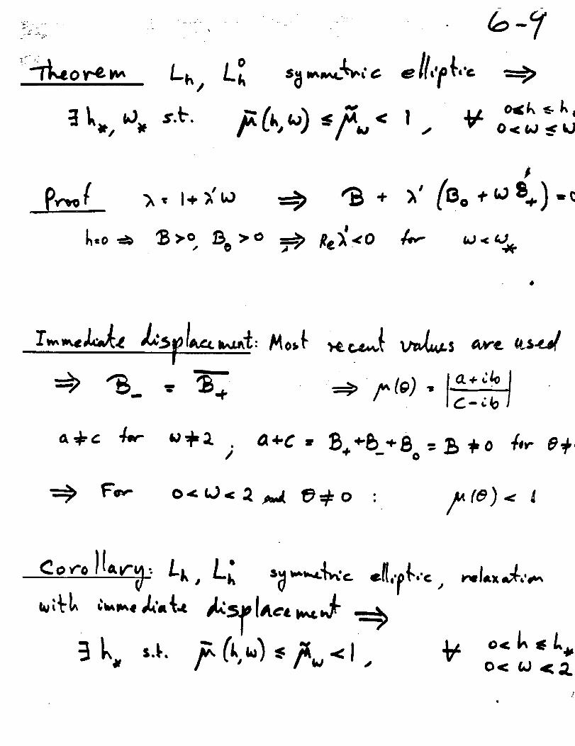
o¢ ¢J.= _. ,j. _=fo : t, ce) ._ 4

/.

• m ii _ ,

,tS c_._ oI

(÷,-_,.,_._ _1o_

\ _Oe" /

! NAVIER-STOKESEQUATIONS,

DISTRIBUTEDRELAXATION

11,,

_I _ Ar' ,IY"

13"

i

/

/

/

T.

o -_ p, .-=4o_L,/

I 1'14,,ILI/"

It

e

.O

0

+_* .+ + , _-"'+ +' . '- -" ':-'. + _J :-+ +_ _.". :_ " •. ' - _ , - _ r '. +++., • - . " +.>+ "_ -. " -:

_ ..... .+ .... +. _,+:?.+'-_ :-++ + - . , .,.+

upst__ gml+_ _;om++

"_ C,.-5

I"-+.+l I

".r + ______.___,...... • "+ -- " .--_--_ ..... -J_J_--J,_"-=-,J

r-" ,_s_,+-e_',++'_op,_,+,+_o+,-.+

L_ ; 0. -_-b-c-_ _ i

_. b .j,. | II I I

,,2._

o

tin,

I

C

_.ol

I

I

I

t

._.+oI _

. Eoo

• St+

. _Jgo

I.Oo_

D

i

.3(_"

,3_

.#_

._81..

.7_._

") _,:,m,.,,'_, 5_le.: I,,A+0

,vt-,,,.+._t,,,,.,,...,+e°+,,_, r.,,.Po,.,+o,,,.+._.+.

P.,,I,,,_,_,.,_.

!

I÷_

rut I÷_bo,

Ax-_s,._,.,,o,sd/.,'lb.,

IIII

/

_eled:;ve '_..e'L_c

8, TRANSONICFLOWPROBLEMS

unto

iimuD

m_

v_

I

0

0II

"f

II

o ,dmID

"'7

I

0_

!

I

Qd

O_mll

,'Ie_idm

II

l

I

6_

..,,.

o ._IUJ

Ik

0 o

o_

B _B

e_

tl II

°,.._

LD

"Z

0

!

l

_m

4

Pql_ 1

I

l

Q

Il• o_

_, II II, ,._.j

3" _ o

0--

,JJ

.°

o.._

I-"LU4-

° "-I

+ _

II . _

°I

-- g

_.... --_c_

•_, _ .z_

o.-_

4-I

°-'I

I,--==J

W

U..

.>-

_J

wo,.

w

I--

1.1.1

I.LUJ

Z0

uJ

ILl

P_0

b

O,_.1t.j")

,....m"q'4

0'_JuJ>ILl

ILlZ

OO ,--,L._

O

.-....'-'1"

• t#3

,...;

ZI.-OO_E

t.,,O

W

ij

J

-..I

ILl'1"

I-,,-LLI

I-- _

Z..%0

r .,.

0C L.t"L.C Lt"0C O_

L._a

C-D. w

"A

X

._1N

3."Y

J

dD

l--

z

0

V

0

_.1

I--II-,-I

z

0¢w,r_

LI_I

_1

U_

II

&

dQ.

t2L,.J

w

fJ_I----I

w

n,,*

I-,.J

LI,..O

>,..r_"

=3

I

,.q,---I

LIJr_:C)

LI_

m

O

I--"O0

X

<:1A<1

ZW

oOO

I_I.-O

ILl

QOc_

ZO

:3=

OO

O

I--

ILl

m

X

<1

oO

CD

V

OO

W

oO!

,-..., LL..I-- CD

I-- 6"_,--, O

O0 W

_-" O--:D ::_..--JCD _'*

CDv I_1_

CO ::,-

W O:3=

I LulX

l---

ILl W

'

0

CDO0

ILl

OO

OO

I'---Z

OID_

U_

O

I--"

ILl

O

O

N

I

f-,

I

-p

q,

"T_

I

t

! t

I"

I

W

Z0

b--<JU-]

-J Z0--4

i,I

--1 O0

J

J

e_

..-i-

I--

I-

v

0.--I

8t,D

.._1

r,,,-l.---

I.J_l

L.I_.I_1...i

I.--0.,.

O0I.J..]

0

b_

II

g

b_

II

V

b_

m

0

II

8

0

Ii

i,Ib--

U-

m

I_U

Z

0

v

0

• ._1

II

W

L]-.m

,3

n,/l 3I _ I'U 'u_

I I I ÷ hi

h.l _ lid IJj /,PI.-,'_ -r '.r t"l _.. t+kl

¢_" I-- o ,IP" ,..+ I-

• i'-- IO m_"_ I .¢"_,

I _ ("'_ _.,./ I

<_ l X • • II l+_J +"',._ I

.,,-I I I II I

I- I I

0 _ ful I'-

I--

3I

tll

7r'l.t_

tL

r_l • ,

Ct_ <.)

I+I

2:

_,_ bJ

>- • • bl

II

-1 mrp,- 1

!

• . _0_

Ill _

_1_ _-_

¢1,' • + •

"_. ,,-I,,-4,,...I

,-, Cq l't) ('tl

• • •

I'll

I

ladC_ I_

.0 n..I

4- ! 4

Ld '..,.J Ldn.I _.-J c,"l

rd OJ _1

4. I I

_ mmm

riJ _rl

! i

I_ bJ

(u c_

÷11 ÷1|

+II ÷II

gg_ 2gg

C_

H

Iv"

F--

0

W

0lad

I.

W!

II!

II

C)

7"b.l(.5

kd

00

(t.

_ I I

_o_ --. 3_g"

_-_ _m_ __0_.

_ +÷I ÷II

_ .oo o.,

,,,_11

0

.1.

I,a°G

I'-

lL

÷

++

+

+

S

I+

!I

+ !

!+

I!

!I

OIf + !

! @ I !! !

I + II !

!I

T

g ,,, g

I _ __q_____

|1||11111111 _-r

,0

2_

,,,4

T

o

0

_25

J_

__0___

__ _1___ _1_

_4____

nJ

('1(X9

_,j(,J

d

_ o

oQ

II

OJ_

II

_1_

2d

mm

illcu fu• q o

i

ulp-

-1- I I

Uibib.IO'p t_ I_r_liu og

_ ,,-4 rU_OQ÷ I !

¢_J III IJ'i

I_- .-_ I_1

I,t. _.1 l::li._l t,f'_ l,Pl

i"-

t',- 17Q_

U'i Id'l Id_

i_. C,- p-

Ill rU O_

_D!

I.d

.,,._ i%1 i'_l

! I IW t.d LLI

_r tD t"-

_ I'Ll i'U

-tl- I !

I,II.d bl

(7_ t"- I21

• • •

P'l Ot U'l

ti3 U_ IJ'l

I

tI .,i ¢t]_

I I i-4 I .41-

-,_ _ I +"i" M bJl,I

i- ¢I _ i_ l.rl

I _ I TI

..,I I I

'0_ II'-- I() t4 fl] (_

IFl

I_ Ctl f'd Ctli-i _i ,r-i .r--_

Il,I

3

•I- I I

fll i'll t'_

4* I Il.l.l I, I t=l

.'_ (,.1) U_ t_

i"l _11 i'd

..l l.i'l I/_ t_l

I,l'l tO t.._t'ki t'tl GI

IbJ

I I I

! ! !

q" _'_ U'_

_d_]

Ihi

CIJLJ'l

4- I ti_ L_ LJ

-i- I I

W LL.I b.i00"!

i'_rl I_') (""1

t,. _"3_

113 I_ ffl

t,i II

t,i t_t_! II

i,t t'4tt tt

.M 0_ f_

_bJ_

Lx-

I I

I

@I

-•+!1

_,_

.=o

b. _-3 ,'_

"-5-

.._q

÷

.#-

-r _7)

b_

TU_= •

_r_"

_r_r

I ILIJ l..l.l(,D t0

r,-(_

•,qr,....i

I I

l,d i.i

C01")O_ "4"

:::)¢_U_ I./I

-_r .st T

cn r31 o)q..4.P.4-...4• o •

w.._r.l I-i

f.9

iLdsr

[.,.

,4 _.- L/I

I I I_W_J

G_P3 _r

+ I I

L_blLd_ U'_ r'-

rlj Cu (u

.iTi -r rrll

h _,"S

U'1 l-n i/_

('..

rIJI'1 [_I I_I I_j

p. ,-_

01Q

0"I'

I I I I IlcJ [IJ I_l I_J I_1

...., fvl -qr ,._..,-, P11

•.-. _ ix) CU ¢.0 _I"

! ¢t,1 e'l _¢_m

--_1 I ÷ ! I

t_. Oi --4 _'_ '_J

_r

i

u_

H

r__E

r_

J<E

I-oi,i

_L

hi

H

t--_J

h,I,h

I

I1II

I

JJJ

(_. r_ [_-

_GOCO

LO

I

_JtO

CII "q" '_

I ! !

_¢tl -

I I |

h.;_

L,I

Z:LI

_J

OL>

U_ (D r'-

PI_P_

r-r-_o3 o3 ,_

L_

I

I I I

! ! !

t_ LM bJU2 _ o'1

-It! L[; U'I

H

H _4

_4 _4

_0_

_l_ L_I _-

_O_

_O+_

r..-

o_ c71 oi

eD_da

t.O

I

_DCO

i I I

l,,J LU l.d

%",,.-.('I

_4' l't.l '_"• • .

+ I IbJhl_J

rJ _J '.J_

,r-,i ,,,.4

I_dt_

I ! !

L_WW

+ ! I

I

bJ

&

L_

0

_(H}4

4_(0_ _

._O_

_O_

•I,(.O: _

1.e ¥_

H

LS

--j-

•,-I.-Ir'-

_IJ(U P1

i_..i_. i..

I

I I i

• I,_ I,_ I_I

"d"

'_r

0

0

o 0!

+ I I 4 t_Ld ljII._J I.I

I

7-

7-

flJ(:Q

r- ÷÷ ,11,.

÷+4-

• ,4-4-

@ 4- I4- I !

4- I iI" ! !

4" ! I+ I

÷ n4. t

@

+4-t"

@4-4"

4"

Lrl

.J • • • • • • • o • • • • • • • , • _ • • • • • • • • • _ • • • _ • • ° • • • • • • t • • • • o ° • • • _ •L_J ! I I I I I I I I I | i I 1 I I t I I I I I I I I ,,_,*,,,,(,,,_,.-4 I-_ I I i I I

0

¢._ ,,3"I..-

.3 ! I lO.

_4"-h"

o

----

A

J_

0...,,,

Itl-.J

0

O0

o,LL.

LL.

_.J

.__]

U

rY"

I,I

O0

0LL-

.J

_.JLLJ

0

0

E_L_

__J

ZLLJ

0C_-

._J__J

LI_

0__JLL.

___0t..,,O

I---

!

0

9, PARABOLICTIME-DEPENDENTPROBLEMS,

................................ ..........................................................

t • • "

Hi

c. ""-

I

v(,,4: _o(,).u=(,,)

"_'m,P.. _ Coo.l_,l..

L=U _ _ Fk - _.._ _;sc._ _.

co_ r$_

a_'l o,a,,, ,.,,, ,.(I levds

3t

la.$

,5

'3

_-Lr

. o2.o_

.oo_

,0o 17

.ooo41

.00o10

.Oooo_C

.OOOOq_

.oo_#

.ooo(,

• Oo o2.0

.00015

,oooot_

.ooooo_o

i

vuu_ _o_.st,,_

8

3_

I_.c/

.._OS

ltoo

Sooo

_oo0

.':lt_ mll '

Lo_-I _e,;_'_ => y_ _,'H e. I. eMJc $ •

q)

I • • • •

_X

A

• • T • * • •• • • o 0 •

• g.®-;. •

,_-u_'_,f,.. s__v'_-.

i0, USINGCOMPOSITEMESHESFORTIME-DEPENDENTPROBLEMS

/0-- /

I_,,f(_er 1_6I,'c

o,- o_er s;.,.,: la.- ,,,.._'_d_

o,,. C.a_-c_,,.._f,..._ ,,,,,.,_,..ds'

/o- _z--

8 RX

cl

dt _ -

-2.-

/0--_

ea.je o'P R,

pv.+_le,,,,.,

oke

...._ -

_e "__ ,,_e _'_.r

foo-,-_ o,l_r/_e.d

_. 4 _I _',__.

w

I:"

t

.¢ a,¢_,-_ct

,i i

c.,,,,'t';',,,_ez _'_s pe..d

m

C_;i_Se

cJoe _c__

._.=__. $ >0 .

_Lt

_amlmmmmmm

f_

0

F

• I ..... -_ II •

I II

mira u Ill ml mm_ Ill i

' _/ l -"I

_r

'-L

• g •

/0 -L

!,,'tet-_ o_-

i

%1 lip

ZlI,,_,,-_Ii-_<l.

+ti"(:T+,,,(',+

_+,,.,I-+.C__,,;,'+'_)

_+p_,+..+,,c,_C,_'_) •

+rm), m +..,t,l+. ,-I" k.

t

A

"l'k,_ e,,Je_I_?p;,,.,_ _.,_',e.

q_

a

AJa '

(x,_) - %(x)

;

o_-e s T

;_ -, I;Ol,,,a_o_.

--|1--

3,.;J _e ,_l,f)"o_;,,-_'l'eby

Lef L,_. /oe "t_e

I

# I

(

IO.-t" _.

gg._e

,,6-,,y-

--'L_I'OS_'_ _0 _I"

0

4",

J k" "

R--

._. ' "" " tT,/_ ,q__ j

1

I

6

,_ ,,_;_ __"_a-- III

• o ,

I

r

",eeP

:)2.q- ;_3_ a__.J

qrs_

11, SINGULARPERTURBATIONMULTI-GRIDTECHNIQUES

- e_._,_d'- "_-

,:.e. _ .?.l,._._.

g _(!

ko{4_,, t..,.,/,, p-._.,

© _-.il _, _(_<)---x:

<o =_ F_

_-3

_..2_

a.o_

_=1o

i i i

ca_

.... --.---- L_

e('Lkev,

o,,. +.+o(++,,.++_)

u:.__,++.++-_(,,,,_£

Co,,,,_k,,,,,c÷c,s.,,,o_ h-+ll,.p+,._ff,+,-,,+o,-+

Lk

L_ _ _

_- e/I,'p _','c.

I_,"o_1{_

0

(_,-) ell_p{,'c.,

!

AeCx) _c_ x

(_,-,+,,,,,._.'l-,..,,+t_,-._ +,+,...+,+.,o+ ,,,..+,,.._,,.,I,+,.o,,,)

12, MULTI-GRIDPROGRAMMING,

f •_-,_/._-.,/---....

eC@l_O l_t

5__5

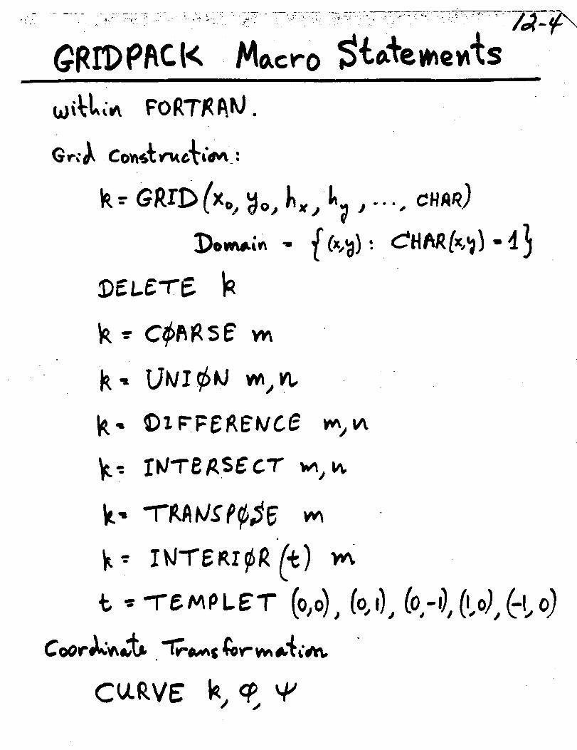
GRll)P_cl4

_oRT_J.

_d>FF I_

"/"y"/Lws _ (y"

,pt_-1"@

e

/.2.-'7

APPENDIX _: SAMPLE MULTI-GRID PRDGRAM AND OUTPUT.

This simple program of Cycle C (written in 1974 by the author at the

Weizmann Institute) illustrates multi-grid programming techniques and

exhibits the typical behavior of the solution process. For a full

description of Cycle C, see Sec. 4 or the flowchart in Fig. i.

The program solves a Dirichlet problem for Poisson equation on a

rectangle. The same 5-point operator is used on all grids. The Ikk 1

residuals transfer is the trivial one (injection), the Ikk_l interpolation

is linear. The higher interpolation (A.7) and the special stopping

criterion (A.16), reco-_ended _or the first [q/p] cycles, are not implemented

here.

For each grid Gk we store both vk and _ (k_l,2,... ,M). For handling

these arrays _ is a/so called vk+M. -- The coarsest grid has NX0 x NY0

intervals of length H0 each. Subsequent grids are defined as straight re-

finements, with mesh sizes H(k) - H0/2**(k-1). The function F(x,y) is the

right-hand side of the Poisson equation. The function G(x,y) serves both

as the Dirichlet boundary condition (#M) and as the first approximation

(UoM) . The program cycles until the L 2 norm of the residuals on GM is re-

below TOL, unless the work WU exceeds WMAX. After each relaxation

sweep on any grid G k, a line is printed out showing the level k, the L 2

norm of the ("dynamic") residuals computed in course of this relaxation,

and WU, which is the accumulated relaxation work (where a sweep on the

finest grid is taken as the work unit).

_T

.... " .i,,,,?-

Note the key role of the GRDFN and KEY subroutines. The first is used

to define a grid (vk) , i.e., to allocate for it space in the general vector

Q (where IQ points to the next available location), and to store its para-

meters. To use grid vk, CALL _Y(k,IST,M,N,H) retrieves the grid para-

meters (dimension MxN and mesh-size H) and sets the array IST(i) so that

k

vij - Q(IST(i)+j). This makes it easy to write one routine for all grids

kv ; see for example, Subroutine POTZ(k). Or to write the same routines

(RELAX, INTADD, RESCAL) for all levels.

To solve an the same domain problems other than Poisson, the only

subroutines to be changed are the relaxation routine RELAX and the re-

sidual injection routine RESCAL, the latter being just a slight variation

of the first.

For different domains, more general GRDFN and KEY subroutines should

be written. A general GRDFN subroutine, in which the domain characteristic

function is one of the parameters, has been developed, together with the

corresponding KEY routine. This essentially reduces the pro crammin_ of

any _ulti-_Tid solution to the _ro_rammin_ of a usual relaxation routine.

fk..._ ik (fk+l _ Lk*i vk+l )k<.l

_k__ik (q,k.l_Ak,.Ivk','l)k_l

NO

v

Figure I. Cycle C, Linear Problems

FROGRA_ CYCLE C

EXTERNAL G,F

CALL MULTIG (3,2,1.,6,.01,30.,G,F|

STOP

END

F_NCTION F(X,Y)

F=SiN (3.* (X÷Y))

RETURN

END

FUNCTION G(X,Y)

G=COS(2.*(X÷Y))

_TURN

END

CYCLE C F 2-/0

Right-hand side of the equation

Boundary values and first approximation

__UBROUTINE

EXTERNal U1,Y

DIMENSION EPS (I0)

DO I K=I ,M

K2=2"" (K-I)

CALL GRDFN (K,NXO*K2*I,NYO*K2+I,H3/K2)

1 CALL GRDFN (K÷M,NXC_K2+I,NYC*K2+I,HO/K2)

EPS (4) =_OL

K:M

_U=O

C_LL PUFF(Z,UI,0)

CALL PU_Y(2*M,F,2)

5 ERR=I.E30

3 E_EP=E_R

CALL RELAX(K,K_M,ERR)

WU=_U+a.*_ (K-_)

WRI_ (6,_) K,ZR_, WU

FORdAT(' LEVEL',I2,' _ESIDUAL _IOR_.='

IF (IRE.LT.EPS(K))GOTO 2

IF (WU.GX.WMAX) EETU_N

IZ (K.E_. 1.0._,. EKRfERRP.LT. .6) GO_O 3

CALL RESCAL (K,K+M,K*M-I)

EPS (K-I) =.3*ERR

K=K-1

C''' PUTZ (K)

GOTO 5

2 IF (K.__C.a) RETUEN

C&LL IN.'_DD (K,K+I)

K=K+I

GOTO 5

_ND

MULTIG (NXO,NYO,HO,M,TOL,WMAX,UI,F)

Multi-grid algorithm (see Fig. i)

, 1PEIO. 3, ' WORK=' , CPF7.3)

SUB_OUTINi GSDFN (N,IMAX,JMAX,HH)

CO_SON/GRD/NST(20) ,i_X(20) ,JMX(23) ,H(20)

DATA __QII/

I_ST (N) --!Q

JMX (N) =J_AX

H (N)=HHI_=IQ÷iMAX*JMAX

F_E_URN

END

Define an IMAX × JMAX

Narray v .

SUB2OUTISE KEY(K,IST,IMAX,JMAX,HH)

CO_|ON/GRD/NST (20),!MX (20) ,JMX(20) ,!! (20)D_MENSION IST(1)

iMAX=IMX(K)

JIIA_=JMX (K)

IS=NST (K) -J_IAX- 1

DO 1 I=I,IMAX

IS=IS + JMAX

ZSr (Z) =IS

HH=H (K) •

RE_URN

_ND

iSet IST such that /_ "_//

vk(I,J)-Q(IST(T) + J),

and set IMAX - IMX(K)

JMAX - JMX(K)

- H(K)

SUBROUTINE PUTF(K,F,NH)

COMaON Q (18000) ,IST(600)

CALL KEY (K,IST,Ii,JJ,H)

H2=H*_NH

DO 1 I=1 ,If

DO I J=l ,JJ

x= (i- I)*HY= (J- 1) _H

Q (!ST (i) +J) =F (X,Y)*H2

EETURN

F_ D

K NH FKv ÷ H(K) •

SUBZOUTINE PUTZ(K)

CO_aON Q (18000) ,IST(200)

CALL KEY (K,iST,II,JJ,H)

DO 1 !=1,If

DO 1 J=l ,JJ

(IST (Z) _J) =0.

RETURN

FND

SUBROUTINE RELAX(K, KRHS,ERR)

CDM_ON Q (18000) ,iS_(200) ,IRHS(203)

CALL KZY (K,IST,II ,JJ,H)

CALL KEY (KEHS,IEHS,II,JJ,H)

rl-r'-- 1

J 1=JJ- 1

E.:.R=0.

DO I i=2,_I

IE =-.=HS (i)

IO=-ST (i)

IM=IST (!-1)

IP=IST(I-1)

DO I J=2,J1

A=Q (I_-J)-Q (IO+J÷l)-Q(IO+J-1)-Q(lif*J) -Q(IP+J)

ERE=ERR+ (A+a.*Q(IO+J))_*2

Q (IO-_J) =-.25.A

ER._.=SQRT (ERR)/H

RETURN

END

A Gauss-Seidel Relaxation sweep

on the equation

K KRHSv _ v

giving

ERR " I iresidualsllL2

SUBBOUTINE INTADD(KC,KF)

C3_?ION Q (18000) ,!STC(2C0) ,_TSTF(200)

CALL KEY (KZ,ISTC,IIC,JJC,HC)

CALL KEY (KF,ISTF,I-_F,JJF,HY)

DO I IC=2,IIC

IF=:*IC- 1

JZ=I

Linear interpolation and addition

_ i_ KCv _v + v

KC

ZFO=ISZF (IZ)IFM=ISTF (IF- I)ZCO=ISTC (IC)ICM=ISTC (IC- I)

DO 1 JC-2,JJCJF=JF÷2

A=.5 _ (Q (ICO+JC)eQ(iCO÷JC-I))

An=. 5_ (Q (IC_+JC) ÷Q (ICM÷JC-1))

Q(IFO÷JF) = Q(IFO*JF) +Q(ICO÷JC)Q (iFM÷J_) = Q(IFM*JF) +.5_(Q(ICO-JC) +Q(ICM+JC))

Q (IFO+JF-I) =Q (iFO÷JF-I) +A

Q(IFM+JF-I) = Q (IFM+JF-I) +.5_(A÷AM)

RETURN

END

SUBROUTINE RESCAL(KF,KRF,KRC)

COMMON Q (13000) ,1OF (200) ,IRF (200) ,I_C(209}

CALL KEY (KF,IUF,iIF,JJF,HF)

CALL KEY (KRF,IRF,IIF,JJF,HF)CALL KEY (KRC,I_C,IIC,JJC,HC)

IIC I=IIC- 1

JJC I=JJC- 1

DO I IC=2,11Cl

ICR=iRC (IC)- = IC-I±F 2_

JF=I

IFR=IRF (IF)!FO=!UF (iF)IFM=IU? (iF- I)

_'_D=IUF (iF+ I)

DO I JC=2,JJCI

JF=JF+2

S=Q (!FOeJF_I)_Q(IFO÷JF-I) +Q(!IM+JF)+Q(IFP+JF)

Q'(iCR÷JC) =_ ._ (Q (!FR+J- _) -S÷_. *Q(iFO+JF) )KETURN

END

Residuals injection

KRC _coarse (vKRF _vKF)v _ Ifine

"_L 6 RESIDUAL NOFM= 2.31aE÷01

EL 6 RESIDUAL N3RM = 2.76_E÷01

EL 5 RESIDUAL NORM = 2.659E÷01

EL 5 RESIDUAL NORM= 2.555E÷01

EL a RESIDUAL NORM = 2.317E+01

"EL _ RESIDUAL NORM = 2.095E÷01

EL 3 RESIDUAL NORM= 1.649E÷01

'?L 3 RESIDUAL NO_M= 1.285E+01

tEL 2 RESIDUAL NORM= 7.626E+00

tEL 2 _ESIDUAL NORM= 3.840E+00

_EL 3 RESIDUAL NORM= 5.058Z+00

r_L _ RESIDUAL NORM= 8.006E,00

/EL _ RESIDUAL NORM= 2.5_5E÷00

/EL 5 RESIDUAL NORM= 9.736E÷00

/EL 5 RESIDUAL NORM= 2._6_E+00

/EL 6 RESIDOAL NORM= 1.06_E÷01

/FL 6 RESIDUAL NORM= 2.4_2E÷00

;EL 6 RESIDUAL NORM= 2.399E.00



/EL a RESIDUAL NO_M= 2.173E+00/EL _ RESIDUAL NO&M= 2.0_3;÷00

;EL 3 RESIDUAL NORM= 1.739E,00

VEL 3 RESIDUAL NORM = I._53E÷00

7EL 2 RESIDUAL NORM = 5.889E-01

VEL 2 RESIDUAL NORM= 6.183E-01

_EL 1 RESIDUAL NORM= 2.760Z-01

VEL I RESIDUAL NORM= 5.170E-02


VEL 3 RESIDUAL NORM= 5._65_-01

VELa RESIDUAL NORM = 7.710E-01

VEL _ RESIDUAL NORM = 1.163E-01

VEL 5 RESIDUAL NORM = 8.657E 01

VEL 5 RESIDUAL NORM = 1.058E-01






VELa RESIDUAL NORM = 8.710E-02

VEL _ RESIDUAL NORM= 7.960E-02


%"V.L 3 RESIDUAL NORM = _ 931E-02




VEL 3 RESIDUAL NORM= 1.9_9E-02

VEL _ RESIDUAL NORM = 3.128E-02

VZL _ RESIDUAL NORM = 8.843E-03

VEL 5 RESIDUAL NORM= 3.710 =_-02

VEL 5 RESIDUAL NORM= 8.a86E-03

VEL 6 RESIDUAL NORM= _.007=-02


WORK=

WORK=

WORK=

WORK-

WORK=WORK =

WORK=

WO RK=WORK=

WORK=

WORK =

WORK=

WORK=

WO R K=

WORK=

WORK=

WORK=WO R K=

WORK=

WOR K=

WORK =

WORK=

WORK=

WORK=

WORK=

WOR K=

WORK=

WOR K=

WORK=

WORK=

WORK=

WORK=

WORK=

WORK=

WORK=

WORK=WORK=

g0 R K=

YORK=

WORK=

WORK=

WOR K=YORK=

WOR K=

WORK=

WOR K=

WORK=

WOPK=WORK=

WO R K=

WORK=

WORK=

WORK=

°I. 000

2.000

2.2502. 500

2.563

_.6252.641

2.656

2.660

2.664

2.680

2.7_2

2.805

3.055

3.305

_.305

5.305

6.305

6.555

6.805

6.867

6.9306.9_5

6.961

6.965

6.969

6.970

6.971

6.975

6.990

7.053

7.1157.3657.615

8.6159.615

10,61510.86511.11511. 17811.2_011.25611.27111.27511.27911.28311.29911.36111. _24

11.67_

11.92_

12.92_

13.92_

OUTPUT

Error reduction by a factor

greater than 10 per cycle.

Each cycle costs 4.3 WU

Insensitivity: Results would

be practically the same

for any .005 < _ < .5

or any 0 < n < .65

PEOGRA_ CYCLE C

EXTERNAt G,F

CALL MULTIG (3,2,1.,6,.01,30.,G,F)

STOP

END

FUNCTION F (X,Y)

F=SiN (3.* (X÷Y))

RETURN

END

CYCLE C

Right-hand side of the equation

FUNCTION G(X,Y)

G=COS(2.'(X÷Y})

_ETURN

ZND

Boundary values and first approximation

SUBROUTINE

EXTERNAL UI,F

DIMENSION EPS (10)

DO I K=I ,M

K2=2 _* (K- I)CALL GRDFN (K,NXO*K2*I,NYO'K2÷I,HD/K2)

I CALL GRDFN (K+M,NXO*K2÷I,NYCSK2+I,HO/K2)

EPS (Z) =TOL

K=M

_U=O

CALL PUTF(M,UI,O)

CALL PUTF(2*_,F,2)

5 ERR=I.E30

3 ERRP=ERI_

CALL RELAX(K,K_M,EER)

• WU=WU÷_.** (K-E)

WRITE (6,4) K,ER_, WU

FORMAT(' LEVEL',f2,' RESIDUAL NOR_--'

IF (ZRR.LT.EPS (K)) @OTO 2

IF (WU.GE.WMAX) RETURN

!Z (K.EQ.I.0R. ERR/_RRP.LT. .6) SOLO 3CALL RESCAL (K,K+_,K*M-I)

EPS (K-l) =.3*ZRF

K=K-I

GOTO 5

2 IF (K.EQ._) RETUP.N_..C_Ll INTADD (K,,K* i)"_

K=K÷IGOTO 5

?-ND

SULTIG (NXO,NYO,HO,_,TOL,_AX,UI,T}

Multi-grid aulgorit_ (see Fig. I)

,1PEI0.3,' WORK=', 0PF7.3)

11t.6

cAu.cAu.

SUBROUTINE gRDF_(N,i_KX,JNAX,HH)

COBMON/GRD/NST (20) ,IBX (20} ,JMX(20) ,H (20}

D_TA IQ/I/

NST (N) =IQ

JZX (N) =JMAX

XD=ZQ+IMAX*JM_XRETURN

END

Define an IMAX x JMAX

array v .

SUBROUTINE KEY(K,T-ST, IZAX,JMAX,HH} ' _ .... _

_ 1

_UBR0ttTZ_E PUTU(_F,KC)COMMON _(18000],IUF(2g0)wIUC(200}CA_L KEY(K_,IUFwI_F,JJF,HF)CALL <EY(KCsIUCeIIC,JJC#HC)O0 I ICml,]ICIFI2*IC=tIF0uZUF(IF)ICO=IUC(IC)jFa-!O0 I JCmt,JJCj_=JV*E .__(ICO+JC)mQ(IFOeJF)

COnTInUE .................._ETURN.END ........

h ,

O00Ut2tO000012200000t230000012a00o00125Cooootaacoooot2?(000_8(OOUUt29(QOOOt_O(

_000_31¢000oi]2(

3UOOt3_'O000t)a0000135

--I-L

III

o

_8UB_O_)iI_E_m_dp_W,(_F,KC)

CO".ON Q(18OOO)elUf(ZgO)wlOC(2OO)

C_LL wEY(_@,IUF,IIF,jJF,MF)C_LL <EY(KC#IIJCeIICejjC#_C)O0 l I.¢=lwllC ..IF=_tIC-IZ_O=IuFCIF)ICO=ZuC(lCI

jFm-l_o0 I JC=t,JJ¢ ....

C0_T_NU_

_. ENO........

.............. QOO_LELO_O00012ZE

__ _000%230. 0000_0.. QOOOI_50

.. Oooot2_O

....... _OL270000_t280

...... 00001290

_oO0_LC.._ 00001]ZC

....... O_OL1tC........... _00_3_(

_00_L35(

COB_{ON/GRD/NST(20) ,INX(20) ,JMX(20) ,! (20|

DiBENSION IST(1)

i_AX=IMX (K)

JIIAX=JMX (K)

IS=NST (K) -JMAX- I

DO I I=I,IMAX

IS=IS + JMAX

ISr (1) =iS

HH=H (K) •EE_URN

END

Set IST such that

vk(I,J) = Q(IST(1) + J),

and set IMAX - IMX(K)

JMAX " JMX(K)

HH - H (K)

12.- 17

SUBROUTINE PUTF(K,F,NH)

COMMON Q(18000) ,15T(600)

CALL KEY (K,IST,II,JJ,H)

H2=H**NH

DO 1 I=I ,II

DO I J=l ,JJ

X= (l- 1) *H

Y= (J- 1) _H

Q (IST (!) +J) =Y (X, Y) _H2RETURN

K NH FKv ÷ H(K) •

SUBROUTINE PUTZ (K)

COMZON Q (18000) ,IST(200)

CALL KEY(K,IST,II,JJ,H)

DO I I=I ,II

DO I J=1 ,JJ

I _ (IsT (1) _J) =o.RETURN

CD_ON Q (18000) ,IS_(200) ,IRHS(203)

CALL KEY (K,IST,II,JJ,H)

CALL KEY (KEHS,IEHS,I_,JJ,H)i1=iI-1

J1=JJ-1

EKR=0.

DO I !=2,II

I_ =.T.RHS (i)-0=iST (!)

Kv ÷ 0

(!-I)= ST _i

DO_I J=2,J_l/_

A=(_I-R-_-Q (IO+J÷ 1) -Q (IO* J- I) -Q (I _.*J) -Q (Tp÷J)

ln'_n ...... _ ..........

::,-- Q(',:,.,,.olERE=SQRT (ERR) /H

F.ErURN

END

A Gauss-Seidel Relaxation sweep

on the equation

_v K - vKRHS

giving

ERR = I lresidualsl IL2

SUBROUTINE INTADD(KC,KF)

COM_ION Q (18000) ,ISTC(2C0) ,ISTF(200)

CALL KEY (KC,ISTC,IiC,JJC,HC)

CALL KEY (KF,ISTF,IiF,JJF,HF)

DO 1 IC=2,11C

_ -_* IC- 1

JF=I

Linear interpolation and addition

_ i_ KCV _V + V

KC

13, THE MULTI-GRIDSOFTWARE

• i

• tS-/

!,

IMPLEMENTATION OF THE MULTI-GRID METHOD FOR

SOLVING PARTIAL DIFFERENTIAL EQUATIONS

Fred G. Gustavson

Mathematical Sciences Department

IBM T. J. Watson Research Center

Yorktown Heights , New York 10598

Introduction: In the MULTT-GR_D method developed by A. Brandt [1], [2] for

solving partial differential equations (PDE), the boundary-value problem is

dlscretized in several grids of widely different mesh sizes. Interaction

between these levels enables one to solve the possibly nonlinear system of

N discrete equations in O(N) operations and to conveniently adapt the dis-

crstlzation (local mesh size, local order of approximation, etc.) to the

evolving solution in a nearly optimal way.

This paper presents an overview of a system of programs that allow a

user to generate and manipulate arbitrary two-dimensional grids. The user

would write a high-level program that would apply the MULTI-GRID theory to

his PDE. In so doing he would call upon system programs that allow him

to conveniently interact between various grids he must generate. In effect,

the system programs convert the FOETRAN language into a language to solve

PDE1svia the MULTX-GRID approach.

Our overview will show how one can effectively represent and manipulate

arbitrary two-dimensional grids. Generalization to three and higher dimen-sions will be mentioned. Section 2 of the paper will describe our data

structure. Section 3 will catalog some of the syst_n programs and the

reason for their existence. Some brief details of their implementation

will be mentioned.

Section 2: A MULTI_GRTD DATA STRUCTURE

The basic tmlt of work in the MULTI-GRID method is the cost of one

relaxation sweep over the finest grid. Sweeping, therefore, must be an

efficient process. Assuming an x-y coordinate system* we will set up

a unlform mesh given by

X m X +iho x

y- yo+Jhy

where Xo' Yo' hx' h Y

specified by integers

(1)

are input parameters and grid points (x,_ are

i and J. We will assume that sweeping is done

in the coordinate direction; so, for example, we may sweep vertical lines

in the negative x direction. One-dimensional storage is very attractive

for storing a contiguous llne of data points since a minimal amount of

pointer structure is necessary to access It quickly. When there are gaps

in the llne we shall represent the data points as a union of intervals; an

interval is a contiguous llne of data points. An example will clarify these

ideas.

More generally, a coordinate system described by two parameters.

6

l 2 3 4 5 6

Figure 1

>

i IR •

Let Xo = Yo 0 and h x 2h - I. _n Figure 1 there are lln_s of dataY

at x values between 2 and 6; i.e., integers in the interval [2,6]. For

each i, 2 < i < 6, there are one or more intervals of grid points; e.g.,

for i - 5 there are two intervals described by integer intervals [2,4]

and [8,11]. (See equation (i) for the relation between numerical value y

and integer value J.)

MULT_-GEID requires four different typ_s of sweeps: They are adaptive

sweeps, partial sweeps, segmental refinement, and selective sweeping.

Because of this we must be able to break up and/or combine grids easily into

other grids. This requires breaking up intervals and reforming them; in

many cases, however, the associated data does not have to be moved. To

facilitate this we propose a more flexible pointer structure, called theQUAD* structure, to describe an interval.

Our data structure for a grid is made of two parts; logical or pointer

arrays to describe grid point (x,y) and data arrays for numerical values

associated with grid point (x,y). Pointer and integer data will be stored

In L space and numerical data in Q space. Assume that our grid is

arranged in lines pointing in the y direction. A quad consisting of four

integer values will describe the first x interval of lines. An x quad

representing interval [a,b] has the following representation:

Qua- ILoc I a I I NEX I

1 2 3 4

The second and third entries describe a and b; i.e., QUAD(2) - a and

QUAD(3) - b-a+l. The third entry of QUAD is the length (number of 7 lines)

of the interval. Entries one and four of QUAD are pointers into L space.QUAD(1) contains the location in L space of the y QUAD describing line

x " xo + ahx. By convention the y QUAD describing llne x , Xo + lhx,

where a < I s b, is located at position LOt + 4(i-a) of L. QUAD(4)

contains the location in L space of the next x quad, if any, of the

QUAD is an abbreviation of quadruple.

I

given interval of lines. The structure of any y QUAD is the same except LOC

points into Q space; i.e., the y intervals refer to grid points• Thus LOC

points at the numerical values that are associated with the given grid point.

Figure _ contains the QUAD structure for Figure i.

L-SPACE

ADDKESS

LOC

a j

8 7

8+4 y+5

8+8 7+11

8+12 y+17

B+16 y+24

8+20 y+7

8+24 y+14

8+28 y+20

QUAD- r

a _ NEXT

2 5 0• • Q"

4 5 0i

3 2 8+20

2 3 B+24

2 3 _+28

2 9 0

7 4 0

8 3 0

8 4 0

ADDRESS

Y

y+4

y+5

7+6

y+7

e"

7+11

y+14

y+17

y+20

,0-24

7+32

Q-SPACE

VALUE

v(2,2)

O

v(2,4)

v(3,1•5)

v(3,2)

V(3,3.5)

-v(4_l)

v(4_4)

v(5_l)

v(S 4)

v(6_1)

v(6_5)

Figure 2

J

If we want to process the points on line i = 5 we access location

L(_) + 4(5-2) " B + 12 in L. The QUAD at location 8+12 tells us that

grid points (5,1), (5,1.5), and (5,2) (see equation (i) to make translation

from J to y) are present; in addition, another interval is located at

L location 8+28. Looking at the QUAD at location 8+28 tells us that

grid points (5,4), (5,4.5), (5,5), and (5,5.5) are present. Also the

numerical values associated with those seven polr._s are stored, in order,

at locations 7+17 to 7+23 of Q space; e.g., v(5,1.5) = Q(7+18).

Section 3: SOME SYSTEM PROGRAMS FOR MULTI-GRID

The System Programs for MULTI-GKID will be classified according to

MULTI-GRID operations as described by the theory [1], [2]. Because of our

choice of data structure, some of these operations will be subdivided into

three parts. These parts are logical creation of pointer structure,

allocation of Q space for numerical values, and putting numerical values on a

grid. Table 1 below details our routines: they are listed as Routines 0

to Routines 4.

Routines 0 - INITIALIZATION I COMPACTIFICATION

INIT

CMPCTL(h)

CMPcrq(k)

FUNCTION/DESCRIPTION

Get parameters from user; set up L and Q space

C_o_bac__ify L space via garbage collection

Compactlfy Q space via _arb_-_e collection

Routines ! - LOGICAL GRID OPERATIONS


LGRDCR

LGRD2F

LCOARS (k, Z)

LUNION (k, &,m)

LSECT (k, & ,m)

LTPOSE (k,&)

L_N_S (k, _ ,m)

DELETE (k)

Create l ogicalgri_ structure given a c_ha_acteristic

function CR(x,y); i.e.,

CR(x,y) = t 0 (x,y) _ grid

1 (x,y) c grid

Create l_oglcal gri_ structure given 2 ftmctions,i.e., Inequalities a £ x _ b and _(_) _ y _ g(x)

describe the boundary curve of the grid

Create l_ogical coarsening of grid k; call _t grid &

Create logical union of two grids; m - ku£

Create logical intersection of two grids, m - kn£

Create logical transpose of two grids; _ = kT:

i.e., Convert a grid stored by vertical lines into

one stored by horizontal lines.

Create logical difference of two grids; m - k-£

Create set of inner points from grid k; £ - INNER(k)

Delete logical structure of grid k

Routines 2 - ALLOCATION OF q SPACE AND INSERTION OF NUMERICAL VALUES

Name FUNCTION/DESCRIPTION

QSPACE (k)

qOFF (k)

POINTO (k, £)

TFERTP (k, £)

PUTF (k,F)

?UTVF (k, VF)

PUTSF(k, J ,F)

PUTC(k,C)

PUTVC (k,VC)

PUTSC(k,J,C).

Allocate storage in O and supply pointers in L for grid

Delete storage in Q previously allocated to grid k.

Poin______the logical structure of grid k intothe numerical storage of grid £

T_.ransfer numerical values from grid k to grid £

T_ransfernumerical values in _rans_osed order from

grid k to grid £

Put function values F(x,y) into the Q space of grid k.

Each grid point (x,y) can have several values associated

with it. A parameter NF st,nding for number of function

values is associated with each grid. If NF > 1 then

PUTF inserts the first function value into Q space

Put vector f_unction VF(x,y) into the Q space of grld k.

Put scalar _unction F(x,y) into the jth function of

grid k; 1 _ J _ NF

Replace function by'constant in the above descriptions

of PUTF, PUTVF, and PUTSC_

Name

CTF(k,£)

FTC(k,_)

LINT(k,£)

Routines 3 - INTERPOLATIONS

FUNCTION/DESCRIPTION -

Transfer coarse values from grid k to fine values on grid £

Transfer _ine values from grid k to _oarse values on grid £

Perform _linear int___erpolation on grid k and put Interpolants

on grid £

Name

KEYS

KEYG

Routines 4 - E_OSURE ROUTINES


Supply user with array JR so that v(l,J) = Q(JR(IR+I)+J).

JR is the KEY array and S stands for single.

Single means each line consists of exactly one interval;

i.e., no continuation strings.

Supply user with several arrays so that user can sweep

easily an arbitrary grid.

Tab le 1

Several of the above routines are easy to implement. The more difficult

ones are in Routines 1 and 3. Since our data structure is predicated on the

interval many of the programs in Routines 1 become simpler if one considers the

corresponding operation for interval. In LUNION, for example, we consider

the problem of finding a union of intervals; i.e., given [al,bl],...,[ai,bi]

and [Cl,dl],...,[cj,dj] we want to form [el,fl],...,[eK, fK] as the union

of these two lines. An efficient algorithm can be implemented to solve this

subproblem; the algorithmcan then be used as a subroutine within LUNION

to find the union of two grids.

A sim/lar algorithm exists for the intersection of two sets of intervals.

However a complication arises which necessitates a type of recursive pro-

Eramming. To see this, suppose [a,b] and [c,d] have a nonempty intersection

[e,f]. If [e,f] represents an interval of lines that are common to both

grid k and grid £ then [e,f] may not be m - kn£. For this to be true each

i, e _ i _ f, must have the property that two lines in grids k and £ associated

with i have a honesty intersection. In general [e,f] is itself an inter-

section of intervals. To find this out we must call the intersection of in-

tervals program for each i; thus we have recursion of depth d equal to the

number of dimensions. This phenomena occurs whenever grid points are deleted

from a region; a change occurs in the quad structure when a part of the region

becomes'empty. Another example is the logical coarsening routine in which a

and H - 2hy, Therefine mesh is replaced with a coarse one; e.g., H x = 2h x . Y

are less points in the coarse grid and possibly the quad structure changes

because of the coarsening.

Probably the most difficult routine to implement is the logical transpose

routine. The problem here is to convert vertical lines into horizontal lines;

i.e., interchange the order of sweeping. We will only meution that our solu-

tion is 0(q lob q) where q is the number of quads. The Io Z q comes in

because it appears crucial to sort separately the end points of the entire setof intervals.

The Routines 3 are difficult because we accept essentially arbitrary grid

configurations. Let K and k represent a coarse and fine grid and assume

that K contains values which we want to interpolate to k. We use billnear

interpolation and everything is okay when there are enough coarse points near

a fine point to interpolate. It turns out, even under reasonable assumptions,

that there are a large number of abnormal cases to consider. Proper pro-

gramming requires code to handle these cases no matter how infrequently they

might occur. It is the cataloging and programming of these cases that makes

the Routines 3 difficult. Also, we want to program so that code goes over to

hAgher order interpolation; e.g. , cubic interpolation.

@

Acknowledsement

The implementation described in this report has benefitted from many

fruitful discussions with Achl Brandt, Allan Goodman and Donald Quarleso

In addition, Allan Goodman has implemented the programs in Routines 2.

References

Brandt, A. - '_ulti-Level Adaptive Techniques (MLAT) I. The Multi-Grld

Method, RC 6026, June 3, 1976.

Brandt, A. - '_ulti-Level Adaptive Solutions to Boundary-Value Problems,

RC 6159, August 20, 1976.

/qVL Tr - GRID

t4Ul.. TE.'_R r.D "__ e e c y

level

(.J s e f C _ //_

_ //o _

I_/em a E Z_

F ;_¢ - t_o- co_rse

'S) P _'-;___orL t.h

/._ -/0

F]ex,' l-b,,needeJ -_ rep,,'ese-'t" (.J_/'for_

_¢ID

_weepsn_,

L.O61C I_L.

6

• 0 °

.T.[IV T G O.P O L P,T t ON vo ;"/: l_ _ ._ I D o -J. Vle _<"_" $ ; _ C

G RID C _E_TXOH

L<_IO Z 1_

(.A t"_ _¢ Pt" I ion./

EY$

._ Y G -USer c_n

/Vu_er;c_. / 4,'ll/Ue.s

sever_ _ zrr_ s so

,j /3-/ _

V"/c'_ _sy.,,

CMPCTL

CI_ PCT Q

I

Q pa.ce

X= c4

"_:S

L. S p_c_" ,¢ (._,,5 )

"u"(.% _.),_.(.%s)

Y :q,

i>,4T_

_ U_qc) Q

LOC ME_T po,',,_,_="l'he_e _re

d'_" "_,p.'- I$ I PI# VtS •

l/if/o'-#

s weep

6t//"

_.. 0_ S _, o_'¢_

Q_/ID s

,rep _ese.'_

d.: d." c_u,___, *7" /'_s_

_e para Jc.e _r_r_J

p_ rJc3

STROCTO_E

t'_ EPeEs _ N "FFe"/'to

_y;Co

yo

JY

• °

I •

_e_ween

( JiJ2) (_O _ D ST_OCTU_

LSEC-T _ - ..{/?Z

C: ,_/9 8

g'o b too 6 _'_,,.

NE_Q ,o/Zo eL _',_

: u_e_f.7

4='_.,s/ ;_'erse=t;o,t C

GCaerd I r..e,_c_]- U Le:, _:3

OF ( e "_V 4J _ _ •

HU_T

T'O 1="JND

[e_-F3

-r o Lo _Es-r- DI_--

u T s Teuc.'rur_ _.

_DC C _ r._ W Jl _n_v'_E

t__-k¢ ,sb_ w'

I

F u _/D _ MEIVT t6 L. I_E L t_ TI O M

,5 =5 - T_.I +_ "r

• _ • - e -6

3: " _"

II • • • t

I •

//L 6 0_ / THm L T PO _k:_/_-_s

tt II

D _ _'r _ ,'_,, "b_fie

o,,t._," _uaJ =_,.,,=_..= ,'.,

Is -r= / +

= Sz-'r_.

t

_oJu lar Z)es,#.

5o _¢oo÷C,,, s _ ( A_ S_ B)

I_=O t=,..,.:_, s:_'_.,...,s,=}8= O [_,a.]

Cos'_

/

LC_OzF

q

fVEE DE D

"i • _ .f

,CEYS

/_EY6. -

2_ j!

5_eep

cao r_ ,_,t÷e

_ _,';_ _'_.,_,_

g z D .)

m rwf

wE

L

L

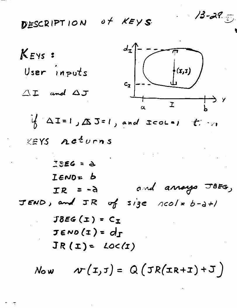
l_'_qC 2 IPT I 0 M A_ y $.).4-.,_q --

p .-_ ,

_:£=1 ,_Z1_3-- I )

._. Y5

z b

,¢coc. -I P,' ";r_

Y

Z_;NO= b

,T_IZ = -;_

s,3¢ ncol= 6-a +l

JSE_ (:z) -- c z

=_,,,o(=) = ot.r3R (.T.) ,= LO<(.T.)

._'-'-_ 1_-. _1

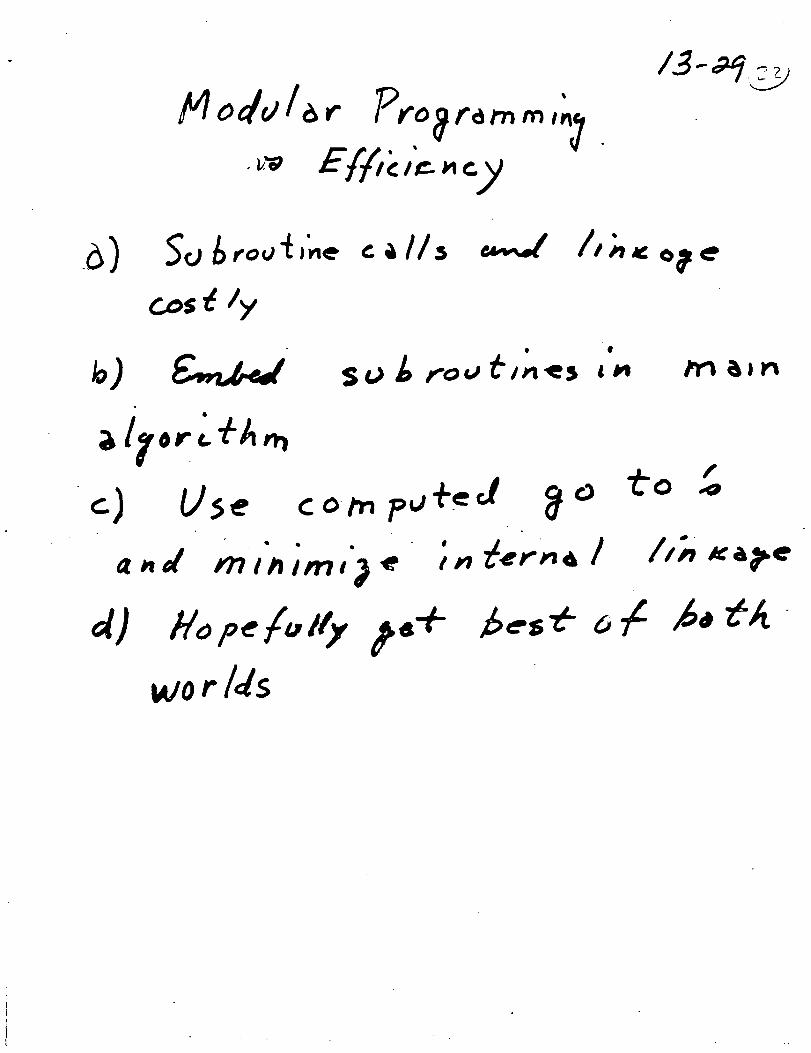
/3- _,:_y

cos _ ly

• • e

c om Fu ÷eJ#

,0

WO r/dS

FOR TRAH- /_ __

_IT Z

3- d,'.' _'t-

_) 3_s were

/so 4_e _-_e

o-/cede

lO l'O#_/"4

e clsl@ f- -C'-o-/_,,d

modv/dr -

"_ Cro¢

F o _.T_N

_ s,e_ b /7

14. MULTI-GRIDPROCESSESON

LARGEARRAYCOMPUTERS

Z-l,/+0

-54-

(e'_/..-t)

(d-Ijj:lj

CELL ARRAY

MEMORY

[ e ii

REGISTERS

ONE CELL

I

p.A0

p._ p.A0

"_ "_ "_ "_ EJ,I 0 -_ _ 0 _.

0

bJ

/',.I

0

0

0

0

,.o

l.n

O0

!

0

w

0

I,,,3

0

0_D

¢)

0

_n

Co

&0

Co

._'_,1 00 _.._ _

E_0

0

0

0

C_

0t_',-.4

0

o

0

0

ocr"

mB

_0 _ _

'_ 0m C

m

C_

,-I I-_

o m_ 0 _

r_ _-_ r_ 0

O.

0

A

0

_-" • 0 _ 0 r_ I"_

;g r_ r_ 0

@ - X "g) f

L t

X - X • X -- X • X

• i,, • • b • ==' b

® • i_ • _- x • @ii, •

• p I- i = II

g • X ,. K " K " X

• w _ v@

.,'_/ , /.L .: ,,4/,,,'o_ .rC • _'-.G.

-d"--->...-T,t't e. ,, a /

o. -w> _ d e/ ,"_c o_,J

1.c"_ea _- .._a z"eJ,po / ,t t ,'an :

a

0

5

!

t_

!

I

0

t_ 0o0

F','ve We, ,A "t"

/# J o /z

.T'a c o/a c"-t- R e_ ,"d ,, ,*I s ;

L--xp ._,_s"c'o_

5"a,,_ J

K_

C:?.o*" ,J-'o'v ,k/a- ,v s_'c

#I"#o -'- _'X t0" ¢"

_o "= /cry X tv -_

"0 = "6,

ef 7_ cO d:'

0

_ &tl-t ¢ #

O,dO

], o-o

0 0

Y[

_" _

,,iCe ÷ /_o dI,,,4/ o _ /_

_-_c o_ c*

"z '7._

L/% 9_o

(M, _,j /, 9"6-o

I_d- /3 /_c/r ..,eo,,_7-_313

15, MULTI-GRID EXPERIENCEON THE MINIMAL-SURFACE EQUATIONS

• • o " • °

. m j _ ._

i

°w

T

p

gi?

i

i

0 !

........ • _ __ • •

• ,w w • •

_D _ _p_ O""• I1_ Q

/_-'2

r,

!

U _-- _r_ _'+V _m

.o

_o

=Z r" +!.. Z._ , .....

= F '_ I

_kO_ • w_R4_l Fo_ IqULTI _ I¢I_.

IdC,YC = S VC,'I,IT mr. II

i.e. -KI,N ; o

•_.aT'lo_" . ._L 14

__ _ +: _'.'. I;,_"+_'0;,__)$oLmT_Bd : U'

....... I'we_ : V ' .. 14: - Z_ U'Pet

so_.u_oAl: 11s Z'_4z_ : V z- _ --_• .. . *. ITTG.

h

(_N--t : _, N-I _ N--t /I N" I

SW_ ncvc .a_.'N V, Pil-i

C

f%

V

t_°j,lt_

wit4"

x_

tQo

_oqF

ape

o tit'_" o

_o

_ -

.i

,,¢

v

,m

v

..... . o

_ mi)'1='S 01_ G_,) "_'k- I,.,..&5). _

_l',-...... -of&

G,G,.

'o¢_ ;ooS "1•o_ .Iq#, "o,o "2•)o:L .S_ "o:_g "5•_)o l':15 -Io=t. I-1t

I , F

•(, J.ll "2 ;.6

"1.lib

"I=1"5

m

| °

16. MULTI-GRIDEXPERIMENTSTO ELLIPTICPROBLEMS

WITHFINITE-ELEMENTFORMULATION

•

°_

_ _.n. _col_s

I •

o_ o,,,

O I"_ • 0,.,,

I

Z

I_l _ ll

_ep_ on

.e rcO r',

_ ul_r,_ri d

-I

-qw.

)

,_tole. L:

,!

na..1-uro.l one s

Cl 761_4 5o1_ _-.I

o.r_c_ rtsic_ _o.I

41' •

,_, _ • _vt

_V m_

l o0 I

o

0 0

0 0

0 0

I

o '_ o '4./

0 o I 0 ¢

o o

o 0 0 I

V

II

.tD.P 4,:_

3.._C."cI.6¢o

.zz3#3 ,.l.¢qV .o53 3.._ q,_f_¢3.7og 3.vo 9 3. _//

0

_3._% 3. 9_B ,,,e..el_3.1all 3._q 3,9, _' 3.q¢,0 3.7#g

i i

t.Z j q

,3.t _.33

3 d_ Its

Co_ff,'c;_ ?:s

_,£_/.,..¢

J.3

j C=o

A.a. d,._,/x-._/:7, C ='0 3,3

3._ ,a2zJJ

33)c33

_._L + +

30 J¢ 3,3

_.o .9.)3

• 50 /. 02.0

.._' _..2_.¢

.8o'/ + j .¢.'1

.gT& + I?.3

.991 + .2. _'

/. .273 - .7

/6-,Z

IO

_.o3o /. 967 ÷3. o

=K..2Jo

S.3oq

#.zl. E>17

*10._

fro.2.

+I0._

¢/. 7

=0

\

._,,_ _-_" o_

- _. _ __.

_., ",,.+ _.-,..__

t

,c,,6 rII "lr t t _ _1

_ x 33

_,_/1_ "__,a,,¢l,on

I0

a.5__.?

'7.1

/6.3

/_3._

_12.8

_7,5

..z5"_.5

i

-I -a. -3Io lO Io

,9."/ _'.q ¢,.I

q.o '/.el _'.1

Ic_ Io Ioii

_,.c_ C,,._. .¢.q_,._ .e._ _.1

I

)m-I )o "'7'

3.(, _t._ _/.I

-G-,I )_'; IoIo

1.1.1 _/.)

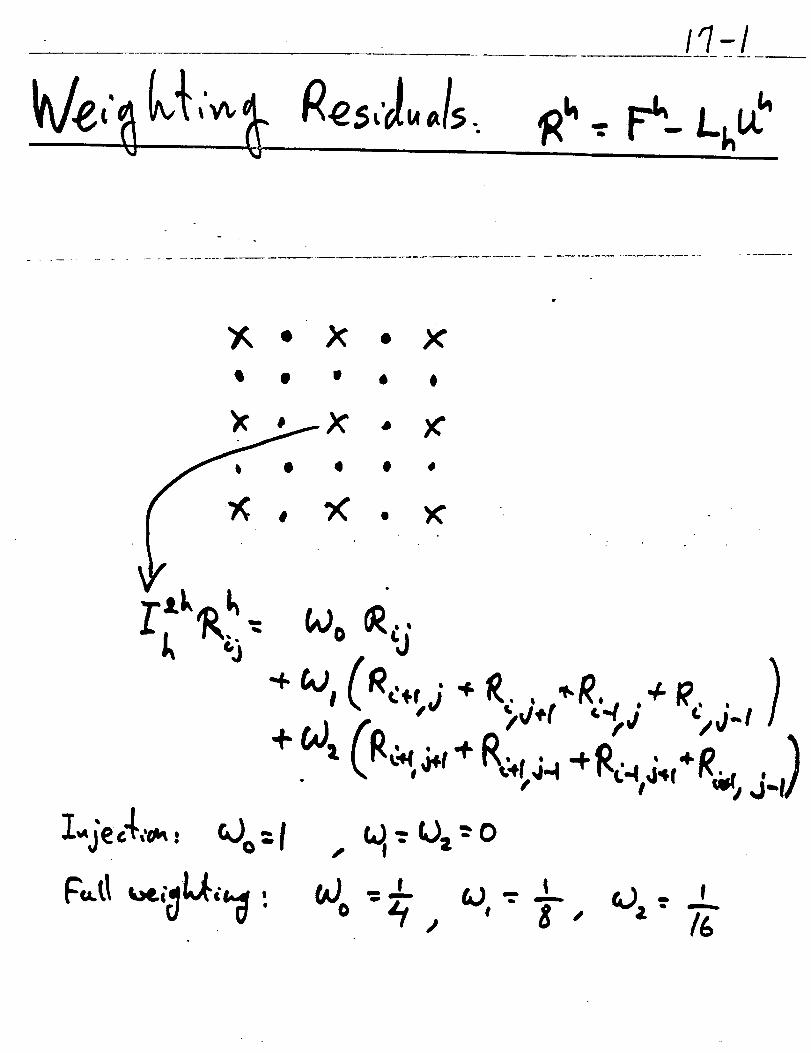
17, RESIDUALWEIGHTING

ANDNON-DIRICHLETBOUNDARYCONDITIONS,

"TU--_ 0

\\

• •

°,i

"_ - h

It

Z'm'l+,e,,v-,:o'v'. • + o.'

.,,.,,t,,.)

, .... I, ....,_ I/,_

I

t

¢

.ol F"

tl

¢,

/,2

.'$ F"

.I I=

•01 I=

.oi F,ol I:_

O.

¢,

_r

t,

-f,d- Jog

.5"1

._'-/

a_¢ it.(,#

"= . • : ¢o|11_1_$ ,

18, DEBUGGINGTECHNIQUES,

_ReLe,_,,..s,'J_-,,_v',,,,,,_ CGC.

_.1,, W_ _' .. ,

k v;,_ ..1, _ ...

'.'-" <<

. |

t_-',\

or',

0_-

'2

ICASEWORKSHOPON MULTI-GRIDMETHODS

JUNE19 - 23, 1978

NAME LIST

Raymond AlcouffeMS 269Los Alamos Scientific Lab

Los Alamos, NM 87545

Alvin BaylissICASEMS 132C

NASA Langley Research CenterHampton, VA 23665

Aivars Celmins

BRL - BMD, Building 394Aberdeen Proving Ground, MD 21005

Jagdish ChandraDirector, Mathematics DivisionU.S. Army Research OfficeP. O. Box 12211

Research Triangle Park, NC 27709

Robert M. BennettMS 340


Marsha BergerSerra HouseComputer Science DepartmentStanford UniversityPalo Alto, CA 94301

Dana Brewer

George Washington University3IS 169

NASA Langley Research CenterHampton. VA 23665

Dennis BushnellMS 163NASA Langley Research Center

Hampton, VA 23665

Fred Carlson

MS 473NASA Langley Research CenterHampton, VA 23665

Hai-Chow Chen

29 Newport KeyBellevue, WA 98006

Ivan ClarkMS 473


Joel Cohen

Department of MathematicsUniversity of DenverDenver, CO 80208

K. R. CzarneckiTABMS 360


Wolfgang DahmenInstitut FUr Angewandte Mathemati_University of Bonn

WegelerstraBe 653 Bonn , WEST GERMANY

-2-

Nathan Dinar

ICASE

MS 132C

NASA Langley Research Center

Hampton, VA 23665

Craig Douglas

Department of Computer Science

Yale Universityi0 Hillhouse Avenue

New Haven, CT 06520

J. P. DrummondMS 168


Douglas L. DwoyerMS 360

NASA Langley Research CenterHampton, VA 23665-

Jim EppersonDepartment of Mathematics

Carnegie-Mellon University

Pittsburgh, PA 15213

F. Farassat

George Washington UniversityMS 461


Donald D. FisherSchool of Math Sciences

Oklahoma State UniversityStillwater, OK 74074

Hartmut FoersterGMD

Schloss BirlinghovenPost fach 1204

D-5205 St. Augustin 1WEST GERMANY

John Gary

Computer Science Department

University of Colorado

Boulder, CO 80309

Gary L. GilesMS 243


Peter A. GnoffoMS 366


Randy GravesMS 366


Anne Greenbaum

1062 Catalina Dr., #58Livermore, CA 94550

Chester E. Grosch

Institute of OceanographyOld Dominion University

Norfolk, VA 23508

Fred GustavsonIBMT. J. Watson Research Center

Yorktown Heights, NY 10598

Mohamed M. Hafez

Flow Research Company21414 68th Avenue South

Kent, WA 98031

Harris HamiltonMS 366


--3--

R. J. HaydukMS 243

NASA Langley Research CenterHampton, Vh 23665

Forrester Johnson

3826 S. W. 313th

Federal Way, WA 98003

D. J. Jones

26 Tiverton Dr.

Ottawa

CANADA

Gershon Kedem

Computer Sciences Department

Math Sciences Building

University of RochesterRochester, NY 14627

E. B. Klunker

MS 360


Jay LambiotteMS 125


Hsi-Nan Lee

Atmospheric Science Division

Building 51

Brookhaven National Laboratory

Upton, NY 11973

Chen-Huei LiuMS 460


Nan-suey Liu



Wayne MastinICASEMS 132C


Stephen F. McCormickDepartment of MathematicsColorado State UniversityFort Collins, CO 80523

David S. McDougalMS 325


Gunter H. MeyerSchool of Mathematics

Georgia TechAtlanta, GA 30332

Ahmed K. Noor



Youn Hwan Oh

103 Sleepy Hollow LaneYorktown, VA 23692

Joseph OligerSerra House - Serra St.

Stanford, CA 94305

-4-

Seymour V. ParterMathematics DepartmentVan Uleck HallUniversity of WisconsinMadison, Wis. 53706

Joe PasciakBrookhaven National LaboratoryBuilding 515Upton, Long Island, NY 11973

T. Craig Poling1645 Ardmore Blvd., Apt. 8Forest Hills, PA 15221

John RadbillJPL 125/1284800 Oak Grove Dr.Pasadena, CA 91103

John W. Ruge200 E. LaurelFt. Collins, CO 80521

Bob SmithMS 125NASA Langley Research CenterHampton, VA 23665

Jerry SouthMS 360NASA Langley Research CenterHampton, VA 23665

Brooke StephensNaval Surface Weapons CenterCode R44Building 427, Room 530White Oak, MD

Robert ReklisLaunch /nd Flight Division •Building 120Aberdeen Proving Ground, MD 21005

J. C. RobinsonMS 395


M. E. Rose

ICASEMS 132C


Hampton, VA 23665

D. H. RudyMS 163


John StrikwerdaICASEMS 132C


Klaus Stueben

GMD, Schloss BirlinghovenPostfach 1204

D-5205 St. Augustin 1WEST GERMANY

Charles SwansonMS 280


Frank C. Thames

Vought CorporationMS 360


--5--

J. W. Thomas

Department of MathColorado State University

Ft. Collins, CO 80521

Deene J. Weidman

MS 190


Hampton, VA 23665

Sylvester ThompsonBabcock & Wilcox CompanyP. O. Box 1260

Lynchburg, VA 24505

Jim WeilmuensterMS 366


J. S. TrippMS 238


Carl Weiman

Department of Math andComputer Science

Old Dominion UniversityNorfolk, VA 23508

John Van Rosendale

31F Digital Computer LabUniversity of IllinoisUrbana, IL 61801

Veer N. VatsaOld Dominion' UniversityMS 163


P. R. Wohl

Department of Math andComputer Science

Old Dominion UniversityNorfolk, VA 23508

Stephen F. WornomMS 360


Robert G. VoigtICASEMS 132C


Eleanor C. WynneMS 340


H. H. Wang1530 Page Mill RoadPalo Alto, CA 94303

E. Carson Yates, Jr.MS 340


Willie R. WatsonMS 460


Warren YoungMS 340


-6-

Csaba K. ZoltaniBMDBallistic Research LabAberdeen Proving Ground, MD 21005

Late Registrants

Lois Mansfield

Department of MathematicsNorth Carolina State UniversityRaleigh, NC 27606

lecture notes of the icase 228 p uaclas 17267 · lecture notes of the icase 228 p uaclas 17267 ......

Documents