lecture notes on damages - s u
TRANSCRIPT
Lecture Notes on Damages
John Hassler
IIES
May 2020
John Hassler (Institute) Lecture Notes on Damages 05/20 1 / 30

Purpose today
Give examples of different approaches to measuring and aggregatingdamages of climate change.
Climate change is a global phenomenon and affects the economy in alarge number of ways.
Two ways to estimate total effects:
bottom up —quantifying all potential effects and summing.reduced form — looking at correlation between natural variation inclimate and variables like GDP, productivity, political stability andothers.
Approaches have different pros and cons. Complementary.
John Hassler (Institute) Lecture Notes on Damages 05/20 2 / 30
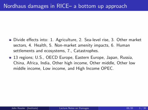
Nordhaus damages in RICE—a bottom up approach
Divide effects into: 1. Agriculture, 2. Sea-level rise, 3. Other marketsectors, 4. Health, 5. Non-market amenity impacts, 6. Humansettlements and ecosystems, 7., Catastrophes.
13 regions; U.S., OECD Europe, Eastern Europe, Japan, Russia,China, Africa, India, Other high income, Other middle, Other lowmiddle income, Low income, and High Income OPEC.
John Hassler (Institute) Lecture Notes on Damages 05/20 3 / 30

Functional specification
For each sector and region, collect studies on how climate changeaffects the economy.
Use studies to specify and calibrate a damage function. This specifieshow climate change (represented by change in global meantemperature) affects damages to output/capital stocks or willingnessto pay for non-market items. All is measured as % of GDP.
For each region, sum over sectors.
Produces a damage function for each region j , D j (T ) .Damages inregion j as a function of the (increase in) the global meantemperature T .
By summing over regions, a global damage function is constructedD (T ) , % of GDP lost as a function of global mean temperature.
John Hassler (Institute) Lecture Notes on Damages 05/20 4 / 30

Example agriculture
Most studied. Damage depends on; CO2, temperature, precipitationand adaptation.Nordhaus summarizes various studies of effects on agriculture
He finds effects that tend to be positive if initial temperature is below11.5 degrees, negative otherwise.
John Hassler (Institute) Lecture Notes on Damages 05/20 5 / 30

Quadratic damage function
The non-monotonic effects of T suggests quadratic damage function
D j (T ) = αjag + α1,ag(T + T j0
)+ α2,ag
(T + T j0
)2Here, superscript j indicates region. T j0 is initial temperature and αjaga country specific constant. α1,ag estimated to be positive and α2,agnegative. Marginal effect of increase in T given by
∂
(αjag + α1,ag
(T + T j0
)+ α2,ag
(T + T j0
)2)∂T
= α1,ag + 2α2,ag(T + T j0
).
Thus, the effect is negative if(T + T j0
)>
α1,ag2α2,ag
.
John Hassler (Institute) Lecture Notes on Damages 05/20 6 / 30
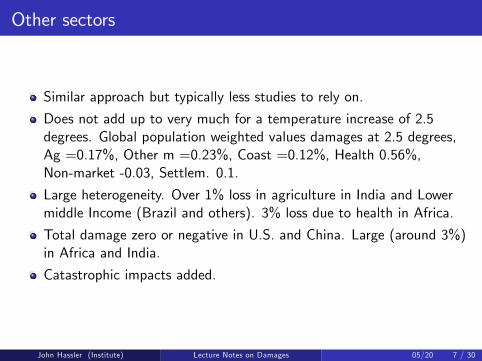
Other sectors
Similar approach but typically less studies to rely on.
Does not add up to very much for a temperature increase of 2.5degrees. Global population weighted values damages at 2.5 degrees,Ag =0.17%, Other m =0.23%, Coast =0.12%, Health 0.56%,Non-market -0.03, Settlem. 0.1.
Large heterogeneity. Over 1% loss in agriculture in India and Lowermiddle Income (Brazil and others). 3% loss due to health in Africa.
Total damage zero or negative in U.S. and China. Large (around 3%)in Africa and India.
Catastrophic impacts added.
John Hassler (Institute) Lecture Notes on Damages 05/20 7 / 30

Catastrophe
Survey to experts. "What is the probability of permanent 25% loss inoutput if global warming is 3 and 6 degrees respectively?"
Varied answers with mean 0.6 and 3.4%. (median 0.5 and 2.0).Arbitrarily doubled and damage increased to 30% globally.
Distributed over regions reflecting different vulnerability.
Assuming risk aversion of 4 translated into willingness to pay to avoidrisk.
Leads to 1.02% and 6.94% WTP for 2.5 and 6 degrees warmingglobally.
India twice as willing, US and China less than half.
John Hassler (Institute) Lecture Notes on Damages 05/20 8 / 30

Nordhaus aggregate damage
Damages as percent of GDP, described by D j (T ) = 1− 11+θj1T+θj2T
2
with region-specific θj s (Blue-USA, Red-Chi, Green-Eur, Black-LI).
0
0.02
0.04
0.06
0.08
0.1
0.12
0.14
1 2 3 4 5 6T
John Hassler (Institute) Lecture Notes on Damages 05/20 9 / 30

Nordhaus (2013)
Goes back to more ad hoc description. Global damages
D (T ) = 1− 11+ 0.00267T 2
≈ 0.023(T3
)2Also allows a term in T 3 producing more convex damages.
Other models have included even larger exponents on T .
The model FUND uses a random exponent from the interval 1.5-3.
Weitzman (2010) has an exponent of 6.8.
Nordhaus stresses that damage function for high temperatures (>3 or4 degrees?) should not be taken very seriously.
John Hassler (Institute) Lecture Notes on Damages 05/20 10 / 30

Damages of carbon (Golosov et al. 2014)
Nordhaus’s aggregate damage function maps temperature intodamages.
Now consider the two steps from increased CO2 concentration (S) tothe change in global mean temperature (T ) and from T to damagestogether. S → T → D.
For the first step S → T use Arrhenius T (S) = 3ln 2 ln
( S+600600
)where
S is GtC over the pre-industrial level (600 GtC). Dynamics aredisregarded.
For the second T → D, we used Nordhaus’global damage functionD (T ).
Together, the two steps are D (T (S)) mapping additionalatmospheric carbon to damages.
John Hassler (Institute) Lecture Notes on Damages 05/20 11 / 30

Simplification of Nordhaus
It turns out that 1−D (T (S)) , i.e., how much is left after damagesas a function of S , is well approximated by the function e−γS forγ = 5.3 ∗ 10−5 (black) and 1−D (T (S)) (red dashed) as seen in thefigure.
0.86
0.88
0.9
0.92
0.94
0.96
0.98
1
0 500 1000 1500 2000 2500 3000S
John Hassler (Institute) Lecture Notes on Damages 05/20 12 / 30

Exponential function very convenient
Define Ynet as output net of damages and Y as gross output,implying Ynet = (1−D (T (S)))Y .Using the approximation (1−D (T (S))) ≈ e−γS ,Ynet = e−γSY .
Then, ∂Ynet∂S
1Ynet
is the marginal loss of net output from additional GtCin the atmosphere expressed as a share of net output.
Using our approximation, we have ∂Ynet∂S
1Ynet
=∂(e−γSY )
∂S1
e−γSY = −γ,i.e., marginal losses are a constant proportion of GDP!
Marginal damage flow independent of GDP and CO2 concentration.
With γ = 5.3 ∗ 10−5 one GtC extra in the atmosphere gives extradamages at 0.0053%. Recall the rate of accumulation of St .
Robust?
John Hassler (Institute) Lecture Notes on Damages 05/20 13 / 30

Ciscar et al. PNAS Feb 2011
Another bottom-up study, but for Europe only.
Sums the impact for 5 types of damages; agriculture production, riverfloods, coastal effects, tourism (market) and health.
Use different high-resolution models 50x50 km, and use distribution ofweather outcomes, not only temperature.
Compare different scenarios for year 2080 to baseline of no climatechange.
For EU as a whole yearly damages equivalent to 1% of consumptionfor 5.4 degree heating in EU. Small positive effects on tourism andsubstantial positive effects on Northern Europe.
Relative to growth rate over 70 years (1.0270 ≈ 4), these effects seemfairly small.
John Hassler (Institute) Lecture Notes on Damages 05/20 14 / 30

Survey Nordhaus and Moffat (2017)
Figure: Metastudy of studies on effects of climate change. Area of ball indicatesreliability judged by Nordhaus and Moffat.
John Hassler (Institute) Lecture Notes on Damages 05/20 15 / 30

Survey Howard&Sterner (2017)
Figure: Metastudie H&S Red dots are non-duplicate studies and line is preferedregression.
John Hassler (Institute) Lecture Notes on Damages 05/20 16 / 30

Reduced form
Idea is to use natural temporal variation in climate and correlate witheconomic outcomes —natural experiments.
Microstudies on agriculture, labor productivity, industrial output,health and mortality, conflicts and stability, crime, .... See Dell, Jonesand Olken, "What Do We Learn from the Weather? The NewClimate-Economy Literature," (Journal of Economic Literature, 2014)
Microstudies yield credible identification but little external validityand no general equilibrium effects.
Fewer aggregate reduced form studies. One of few: Dell, Jones andOlken. American Economic Journal: Macroeconomics (2008).
Monthly data on weather from 1900, 0.5 degree spatial resolution(interpolation) (use 50 last yearly obs.). Economic data from PennWorld Tables, 136 countries.
John Hassler (Institute) Lecture Notes on Damages 05/20 17 / 30

Blue circle (red plus) is mean temp in 1950-1959(1996-2005). Gray lines is range of annual
temperature over sample period.John Hassler (Institute) Lecture Notes on Damages 05/20 18 / 30
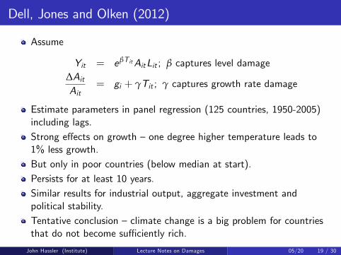
Dell, Jones and Olken (2012)
Assume
Yit = eβTitAitLit ; β captures level damage∆AitAit
= gi + γTit ; γ captures growth rate damage
Estimate parameters in panel regression (125 countries, 1950-2005)including lags.Strong effects on growth —one degree higher temperature leads to1% less growth.But only in poor countries (below median at start).Persists for at least 10 years.Similar results for industrial output, aggregate investment andpolitical stability.Tentative conclusion —climate change is a big problem for countriesthat do not become suffi ciently rich.
John Hassler (Institute) Lecture Notes on Damages 05/20 19 / 30

Kahn, Mohaddes, Ng, Pesaran, Raissi, Yang (2019)
Panel estimate (174 countries, 1960-2014) of
∆yi ,t = ai +p
∑l=1
ϕl∆yi ,t−l +p
∑l=0
β+l ∆ (Ti ,t−l − T̄i ,t−l )+
+p
∑l=0
β−l ∆ (Ti ,t−l − T̄i ,t−l )− + εi ,t ,
where ∆yi ,t is output growth in country i , Ti ,t is yearly averagetemperature in country i and T̄i ,t−l is 30 year average.Results:
Increasing and decreasing temperature has same negative effect. Statusquo bliss.No significant difference between rich and poor, or hot and cold.Effect non-trivial. 0.01 degrees per year, reduces growth by 0.06%(with no rebound).BAU leading to 4 degrees higher GMT by 2100 (0.04 degrees/yearincrease) reduces global GDP by 7%.
John Hassler (Institute) Lecture Notes on Damages 05/20 20 / 30

Temperature - GDP with high resolution data
Unit of analysis: 1◦ × 1◦ global grid (land). 19,000 regions (cells).Nordhaus G-Econ database: GDP and population for all cells in 1990,1995, 2000 and 2005.
Produces nice charts!
John Hassler (Institute) Lecture Notes on Damages 05/20 21 / 30

John Hassler (Institute) Lecture Notes on Damages 05/20 22 / 30
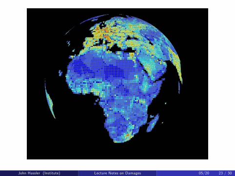
John Hassler (Institute) Lecture Notes on Damages 05/20 23 / 30
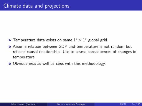
Climate data and projections
Temperature data exists on same 1◦ × 1◦ global grid.Assume relation between GDP and temperature is not random butreflects causal relationship. Use to assess consequences of changes intemperature.
Obvious pros as well as cons with this methodology.
John Hassler (Institute) Lecture Notes on Damages 05/20 24 / 30

Share of Global GDP vs Yearly Mean Temp
John Hassler (Institute) Lecture Notes on Damages 05/20 25 / 30
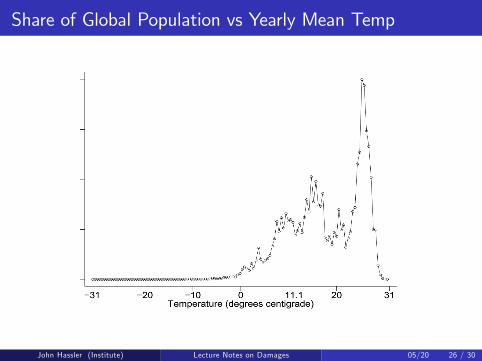
Share of Global Population vs Yearly Mean Temp
John Hassler (Institute) Lecture Notes on Damages 05/20 26 / 30

Climate change affects regions very differently. Stakes big at regionallevel.
Though a tax on carbon would affect welfare positively in someaverage sense, huge disparity of views: 55% of regions hurt, 45%benefit from climate change.
Strong migration pressures from climate change.
John Hassler (Institute) Lecture Notes on Damages 05/20 27 / 30

Dangerous to use model-free econometrics?
A model is a way of imposing discipline on predictions.Predictions based on empirical analysis without model can bedangerous.Recent example: Burke, Davis, Diffenbaugh, Nature 2018.Estimates effects of temperature on national GDP per capita growthrates from a panel regression with yearly observations on growth andtemperature (country fixed effects and quadratic time trends).
∆yi ,t = β1Ti ,t + β2T2i ,t + µi + νt + γ1t + γ2t
2 + εit
Finds β1 > 0, β2 < 0. Growth increases (decreases) in temperature iftemperature is below (above) 13 degrees. Uses the estimates toproject the long-run consequences of global warming.Gives nonsensical results out of line with growth facts.I used their estimates to look at consequences for EU of an increasein the Global Mean Temperature by 2.5 degrees (peaking at 2080).
John Hassler (Institute) Lecture Notes on Damages 05/20 28 / 30

Consequences of 2.5 degrees increase in GMT for EU15
John Hassler (Institute) Lecture Notes on Damages 05/20 29 / 30

Conclusion
Empirical support for substantial effects on the economy from climatechange.
Effects can be large in particular regions.
Evidence does not clearly point towards very large aggregate effectsfor moderate heating (<3 degrees). But substantial uncertainty andheterogeneity.
Very little is known for more extreme scenarios.
At least for moderate heating marginal damage per unit of extra tonin atmosphere may be approximately constant.
Much to be learnt from further research.
John Hassler (Institute) Lecture Notes on Damages 05/20 30 / 30