lecture notes on game theory - university of...

LECTURE NOTES ON GAME THEORY

September 11, 2012

Introduction:So far we have considered models of perfect competition and monopoly which are the two

polar extreme cases of market outcome. In models of monopoly, the notion of an equilibriumis straightforward: A firm maximizes profits.

Most industries have more than one firms but are still not perfectly competitive. In otherwords, they are oligopolies. In models of oligopoly, the notion of an equilibrium is morecomplicated since a firm’s profit depends not only on its own price but also on its rival’sprices. We now turn to game theory which is the formal study of interactions between smallnumber of agents. This will provide us with a guide fir how to think about equilibrium andoutcome with oligopoly.

There are two type of games- simultaneous (normal form) and sequential1 (extensiveform) games. Normal form games are games when the move of agents are simulta-neous. Later we will look at extensive form games, which allow for agents to movesequentially.

The following are three examples of game:(i) Here is the representation of a normal form game called the Prisoner’s Dilemma.

Player 2

Player 1

Cooperate DefectCooperate (10,10) (-1,11)Defect (11,-1) (0,0)

Here is how to read a normal form game: Inside the matrix are the payoffs, firstto agent 1 then to agent 2. On the left are the strategies of agent 1. On thetop are the strategies of agent 2. Payoffs are a function of an agent’s strategiesand of its rival’s strategies.Within this framework of a normal form game, we would like to develop a notionof an equilibrium. The first coherent notion of equilibrium for normal formgames and one that remains powerful today- is Nash equilibrium. Developed inthe 1950s by the now Nobel laureate John Nash., this concept allows us to thinkabout equilibria in economic models where they may be gains from cooperationas in the Prisoner’s Dilemma.A Nash equilibrium (NE) is a set of strategies, one for each players, such thatno unilateral deviation is profitable.For the Prisoner’s Dilemma game, the 4 strategy sets are:{C,C} : Both players have incentive to deviate ⇒ Not a NE

1Such as in predatory pricing1

LECTURE NOTES ON GAME THEORY 2 of 25

{C,D} : Player 1 has incentive to deviate to increase the payoff from -1 to 0 ⇒it’s not an NE.

{D,C} : Player 2 has incentive to deviate to increase the payoff from -1 to 0 ⇒it’s not an NE.

{D,D} : No players have incentives to deviate ⇒ NE

From the Prisoner’s Dilemma example, we learned that:(a) This game has a unique NE.(b) The NE in this game is not Pareto optimal.

(ii) Let’s consider another example of a normal form game. The game is calledChicken Game. In the game of chicken, both players want to show that theyare tough. They are driving towards each other on a road. The one who choosesto pull over is the chicken and suffer a loss of face. Of course, if neither pullover, then both individuals will die and get an even worse payoff.

Player 2

Player 1

Drive Pull overDrive (-10,-10) (7,-5)Pull over (-5,7) (0,0)

For the Chicken game, the 4 strategy sets are:{D, D} : Both players have incentive to deviate ⇒ Not a NE{D, P} : Neither player has incentive to deviate ⇒ NE.{P, D} : Neither player has incentive to deviate ⇒ NE.{P, P} : Both players have incentives to deviate ⇒ Not a NE

Lesson from the Game of Chicken: NE is not necessarily unique and hence itdoesn’t always tell us what will happen, it only rules out some possibilities. Infact this example is probably typical of some negotiation situations, where NEcannot tell us who will come out ahead.

(iii) Consider a final game- Matching Pennies. In this game both players simulta-neously choose whether to put a penny as head or tail. If both pennies match,the player 1 gains $1, otherwise player 2 gain $1.

Player 2

Player 1

Head TailHead (1,-1) (-1,1)Tail (-1,1) (1,-1)

For the Matching Pennies game, the 4 strategy sets are:{H, H} : Player 2 has incentive to deviate ⇒ Not a NE{H, T} : Player 1 has incentive to deviate ⇒ Not a NE{T, H} : Player 1 has incentive to deviate ⇒ Not a NE{T, T} : Player 2 has incentive to deviate ⇒ Not a NE

Prepared by Chrystie Burr


Lesson from the Matching pennies game: There is no NE where everyone picksone strategy. This is true of most zero sum games. We will detail next classthat in this case people can choose mixed strategies.

Elements of a Game:• Players• Strategies/Actions• Payoff functions

Definition of Nash Equilibrium: Agents who are acting as a profit maximizer inter-acting with other agents have no unilateral incentive to deviate from the equilibriumstrategy.



September 13 2012 continue on Game Theory

On mixed strategy equilibrium: Let’s continue with the matching penny game, whichis really a metaphor for most zero-sum games. (Note again that the equilibrium isin terms of strategy not payoff. For example The Nash equilibrium of the Prisoner’sdilemma game is that both players choose to Defect).

Player 2

Player 1

Head TailHead (1,-1) (-1,1)Tail (-1,1) (1,-1)

We showed last class that there is no NE to this game where the agents pick one ofthe strategies H or T. In this type of situation, one can define an Nash equilibrium inmixed strategies. The earlier equilibria that we defined on Tuesday are called purestrategy Nash equilibria. A mixed strategy equilibrium specifies that players ”flipa coin” and randomize over strategies. E.g. for matching pennies, a potential mixedstrategy is to roll a dice, choose head if it is 1 or 2 and choose tail if it comes out3, 4,5, or 6. It turns out that this game has a unique mized strategy NE, and as weshowed in the last class, there is no pure NE in the matching pennies game.

In this case, the mixed strategy NE is:

payer 1 plays

H

1

2the time

T1

2the time

and player 2 does the same.It’s easy to see that the chance of landing on any of the 4 boxes of the outcomes

is 14. Any deviation, e.g., playing H 2

3of the time (as our dice example) will leave

the agent with a payoff of 0/ Hence, no unilateral deviation is profitable, and thisstrategy profile is a NE.

On extensive form game: motivating example of predatory pricing game. Up tonow, we have considered normal form game, which do not specify the order at whichactions occur, and hence are most useful with simultaneous moves. Sometimes, it’sgoing to be necessary to understand the order of actions as this may affect what wethink happens.

Consider the case of predatory pricing game timing:(i) A potential entrant decides whether to challenge the incumbent by entering.

(ii) The incumbent decides whether to fight the entrant by starting a price war oraccommodate only if the potential entrant has entered. Here is the extensiveform of the game which we also called a game tree:

For every extensive form game, we can find a unique normal form game that repre-sents the same situation. However, the normal form representation is incomplete, asit doesn’t tell us the order of the actions: did the entrant move first, the incumbentmove first, or did they move together? We need the extensive form game to tell us.



Figure 1. Game tree representative of the predatory pricing game

Let’s write down the normal form representation of the game of predation.

Player 2 (Incumbent)

Player 1 (Pot. ent)

Fight AccomodateEnter (-4,-4) (4,4)Stay out (0,10) (0,10)

Note that if the potential entrant stays out, the decision of fight or accommodate isirrelevant: that node of the game tree isn’t even reached.

Let’s consider the NE of this game.

{Enter, Fight} : Either players have incentive to deviate ⇒ Not a NE{Enter, Accommodate} : Neither player has incentive to deviate ⇒ NE.

{Stay out, Fight} : Neither player has incentive to deviate ⇒ NE.{Stay out, Accommodate} : Player 1 has incentives to deviate ⇒ Not a NE

Note that we have 2 NE, but one of them is not ver appealing: {Stay out, Fight}looks like an equilibrium only because we have not put in the timing of this game.Otherwise, we would recognize that once the potential entrant has entered, it doesn’tmake sense to fight.

Because the NE concept doesn’t seem very useful for extensive form games, wetypically use a different solution concept, call backward induction. We saw graph-ically how to do backward induction. It involves starting at a terminal node of thegame and eliminating strategies that are dominated. Then we worked backwards tothe beginning of the game, iteratively eliminating the dominated strategies, until wefind the exact set of strategies that are not iteratively dominated. In this case, theonly strategy profile that survives backward induction is {Enter, Accommodate}.

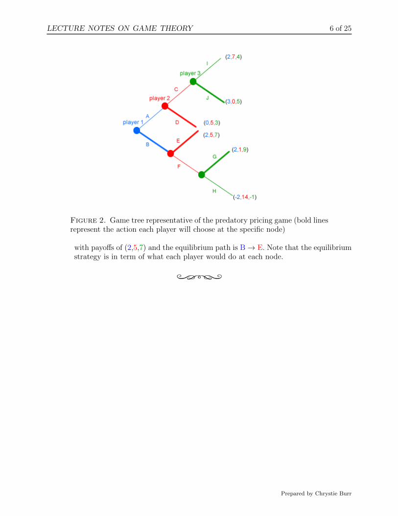
Last example of the extensive form game. We gave just now an example of a moreinvolved game. But we can see that it’s straghtforward to use backward inductioneven for this game. The equilibrium strategy for each player is: {B, {D, E },{J, G}}



Figure 2. Game tree representative of the predatory pricing game (bold linesrepresent the action each player will choose at the specific node)

with payoffs of (2,5,7) and the equilibrium path is B→ E. Note that the equilibriumstrategy is in term of what each player would do at each node.



September 18, 2012 continue on extensive form game

On information structure of the extensive form game:One last point regarding extensive form games. Up to now, we have considered

only extensive form game where agents move sequentially. It is possible to modelextensive form games with simultaneous move. In this case, we put a big bub-ble around nodes to indicate that the agent can’t distinguish between nodes in abubble. This allows us to represent simultaneous games or games that are partlysimultaneous.

Figure 3. The bubble represnt that player 2 can’t tell whether player 1 played C or D

Although this game looks sequential, it is essentially simultaneous and is in factthe prisoner’s dilemma. Or consider another game (see Fig. 4), player 2 doesn’tknow if player 1 played C or D. But she does know if player 1 played E or (C, D).



Figure 4. Last example

Cournot Competition

We are now going to analyze the Cournot model. The Cournot model is the first economicgame theoretic model and dates to the early 19 century. The model is as follows: Thereare 2 firms, each of which produce the same homogeneous product (Later we will expand tothe case when there are more than two firms.) Each firm simultaneous chooses a quantity.Denote the quantities q1 and q2 respectively. The total quantity is Q = q1 + q2. Demand isgiven by Q(P ) which is some function often similar to demand curves we have used before.The goal of the firms is to maximize profits. We solve for the Nash equilibrium, also calledthe Cournot equilibrium out of historical reason.

Let’s proceed with the same example as the monopoly case. Q(P ) = 10−P and MC(Q) =4 for both firm 1 and 2. Solve for the best response of firm 1 and 2. The best response is afunction of the other player’s action.

By the Nash equilibrium definition, we want to solve for the (q1, q2) such that no unilateraldeviation is profitable. This means that we will condition on q2 and find out what q1 leavesfirm 1 feeling like she doesn’t want to deviate. We will then go back and do the same forfirm 2. We will then combine them to get an answer. For now, consider a given q2 and we’regoing to solve firm 1’s optimal q1 which is equivalent to saying that no unilateral deviationis profitable.

Profits=Price × my quantity - my total costLet’s write the demand curve as P = 10−Q, which is the inverse demand curve. Formally

Π1(q1; q2) = (10−Q)q1 − 4q1

= (10− q1 − q2)q1 − 4q1(0.1)

This is similar to the monopoly case except that q2 is in the expression. Let’s differentiateto find the optimal q1:

dΠ1

dq1(q1, q2) = (10− q1 − q2) + (q1)(−1)− 4 = 0



at the optimal quantity. Collecting terms, we have

6− 2q1 − q2 = 0

⇒ q1 =6− q2

2

This defines a reaction function. It says what firm 1 should do as a function of what firm2 is doing. Suppose firm 2 chooses: Note that if q2 = 0, then your rival doesn’t produce

Table 1. Reaction function table of firm 1

Firm 2 chooses: Firm 1 should choose:q2 = 0 q1 = 3q2 = 1 q1 = 5/2q2 = 2 q1 = 2q2 = 3 q1 = 3/2q2 = 4 q1 = 1q2 = 5 q1 = 1/2

at all and you have the incentives of a monopolist. Thus q1 = 3 in this case, which is themonopoly quantity. Now to solve the equilibrium, we need to update what firm 2 does as afunction of firm 1’s quantity.

Π1(q1; q2) = (10−Q)q2 − 4q2

= (10− q1 − q2)q2 − 4q2

= 6q2 − q1q2 − q22

(0.2)

dΠ2

dq2(q1, q2) = 6− q1 − 2q2 = 0

q2 =6− q1

2(0.3)

which is firm 2’s reaction function. Let’s plot out this reaction function: It’s probably easiest


q1 q20 31 5/22 23 3/24 15 1/2

to see the uniqueness from the graph. The only point at which the reactioni function touchis q1 = q2 = 2. This is the only NE. The final way that we will solve for the NE quatities isusing the algebra of simultaneous equations systems. Reaction functions are:

Firm 1 : q1 = 6−q22

Firm 2 : q2 = 6−q12



Figure 5. Graphical solution of the Cournot duopoly example

Substituing Firm 2’s output into firm 1’s reaction curve gives

q1 =6− 6−q1

2

2

q1 =6 + q1

44q1 − q1 = 6

q∗1 = 2 (= q∗2)



1. September 20, 2012

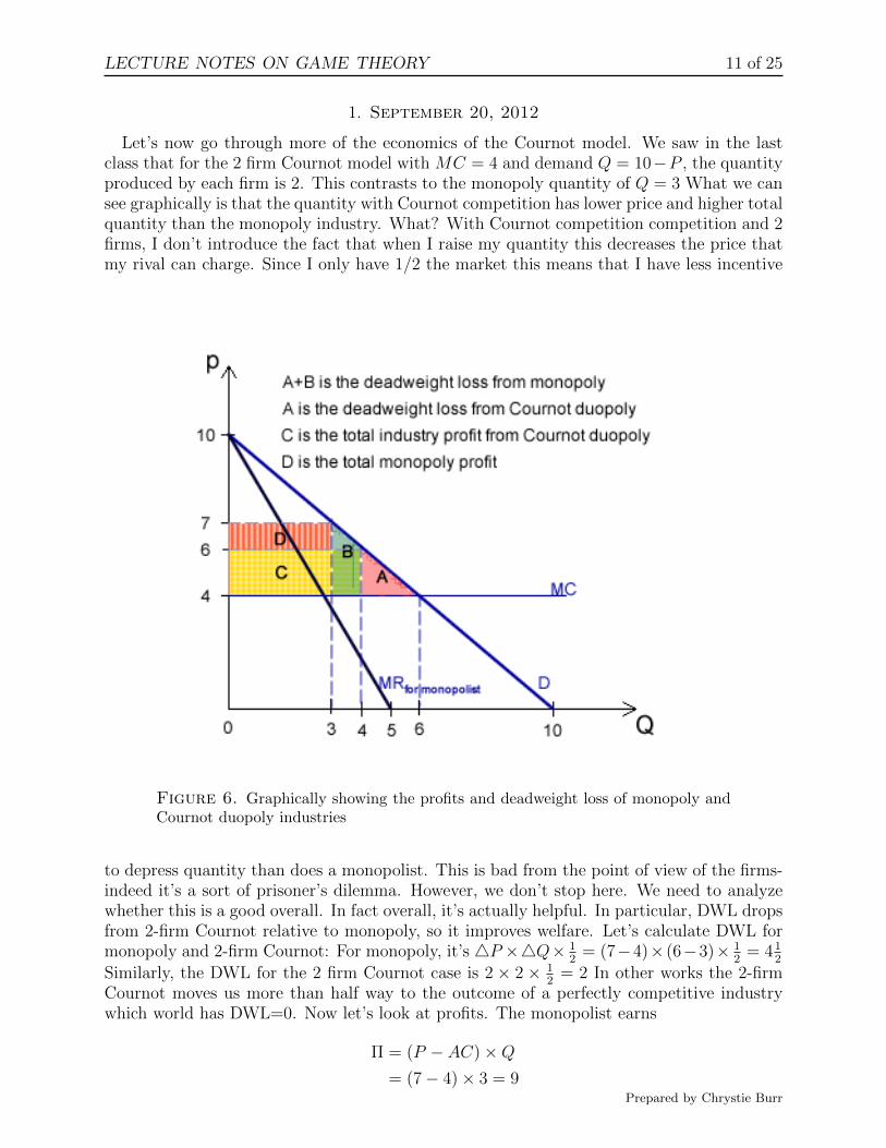
Let’s now go through more of the economics of the Cournot model. We saw in the lastclass that for the 2 firm Cournot model with MC = 4 and demand Q = 10−P , the quantityproduced by each firm is 2. This contrasts to the monopoly quantity of Q = 3 What we cansee graphically is that the quantity with Cournot competition has lower price and higher totalquantity than the monopoly industry. What? With Cournot competition competition and 2firms, I don’t introduce the fact that when I raise my quantity this decreases the price thatmy rival can charge. Since I only have 1/2 the market this means that I have less incentive

Figure 6. Graphically showing the profits and deadweight loss of monopoly andCournot duopoly industries

to depress quantity than does a monopolist. This is bad from the point of view of the firms-indeed it’s a sort of prisoner’s dilemma. However, we don’t stop here. We need to analyzewhether this is a good overall. In fact overall, it’s actually helpful. In particular, DWL dropsfrom 2-firm Cournot relative to monopoly, so it improves welfare. Let’s calculate DWL formonopoly and 2-firm Cournot: For monopoly, it’s 4P ×4Q× 1

2= (7−4)× (6−3)× 1

2= 41

2

Similarly, the DWL for the 2 firm Cournot case is 2 × 2 × 12

= 2 In other works the 2-firmCournot moves us more than half way to the outcome of a perfectly competitive industrywhich world has DWL=0. Now let’s look at profits. The monopolist earns

Π = (P − AC)×Q= (7− 4)× 3 = 9



Each Cournot firms earnsΠ = (P − AC)× q1

= (6− 4)× 2 = 4

So total profit is 8 (note that it’s less than monopoly profit). Probably the biggest deviationof the Cournot model from the real world is that we have assumed a model of homogeneousproducts. In a real world duopoly, like Coke and Pepsi, some people prefer Coke and otherPepsi. This then implies that competition will be less stark: if Coke raises its quantity, itwill have to lower price more than in our model to get Pepsi drinkers to switch. Hence, itwon’t raise its quantity as much as we predict. Let’s now consider a slightly more generalmodel. The aim will be to evaluate how industry performance varies as we allow for moreand more firms.

Instead of assuming that demand is

Q = 10− P,Let’s now use

Q = a− P,Similarly, instead of TC(q) = 4q, let’s use TC(q) = cq so MC = c. More importantly,instead of having 2 firms. Let’s allow N ≥ 2 firms. Let’s start by writing profits for firm 1:

Π = market price× q1 − c× q1= (a−Q)× q1 − c× q1= (a− q1 − q2 − ...− qN)× q1 − c× q1

Let’s now differentiate the profit function in order to find the optimal reaction function forfirm 1, exactly as we did in the 2-firm Cournot case.

dΠ(q1)

dq1= q1 × (−1) + a− q1 − ...− qN − c = 0

at the optimum.

⇒ a− q2 − q3 − ...qN − c = 2q1

⇒ q1 =a− q2 − ...− qN − c

2This is very similar to the reaction function for the 2-firm Cournot case, which was

q1 =a− c− q2

2

Let’s solve for the Cournot equilibrium quantities. Here we will use the fact that costs arethe same across firms to impose that

q1 = q2 = ... = qN ,

or that quantities are the same across firms

⇒ q1 =a− (N − 1)q1 − c

2

We want to solve for q12q1 + (N − 1)q1 = a− c⇒ (N + 1)q1 = a− c

⇒ q1 =a− cN + 1



Because all firms produce the same, total industry output is

Q =N

N + 1(a− c)

Let’s now evaluate what happens to q1 and Q as we raise N: What we can see is that as we


N q1 Q

2 a−c3

23(a-c)

3 a−c4

34(a-c)

4 a−c5

45(a-c)

5 a−c6

56(a-c)

......

...

1000 a−c1001

10001001

(a-c)

get more and more firms in the industry, Q approaches a − c, even though each individualfirm produces less and less. As we’ll see on Oct.2, perfect competition has Q = a− c. ThusCournot competition with many firms approaches perfect competition.



October 2 2010 Lecture on Cournot and Stackelberg model

At the end of the class of Sept. 20, we considered Cournot models with more than 2firms. The general intuition for what happened is that as the number of firms got larger,industry quantity approached perfectly competitive level, industry profits approached 0,prices approached MC and individual firm quantity approached 0.

Let’s replicated the same table form the end of last class adding in price and profits.TC(q) = cq, Demand curve of Q(P ) = a − P ⇒ P = a − Q. Thus we see that profits

Table 4. A individual Cournot Firm’s quantity and profit table

N q1 Q P Πi

1 a−c2

12(a-c) 1

2(a+c)

(a−c2

)22 a−c

323(a-c) 1

3a+2

3c

(a−c3

)23 a−c

434(a-c) 1

4a+3

4c

(a−c4

)24 a−c

545(a-c) 1

5a+4

5c

(a−c5

)26 a−c

656(a-c) 1

6a+5

6c

(a−c6

)2...

......

......

1000 a−c1001

10001001

(a-c) 11001

a+10001001

c(a−c1001

)2per-firm one deciding in the number of firms. For out earlier example with a = 10 andprofits are Thus for we have considered industries without any fixed costs. Suppose nowthat we add in a fixed cost, as that TC(q) = cq + FC. Suppose we take the same exampleof D = 10, c = 4 but now add in FC = 2. How many firms will choose to produce?

We can see that for FC = 2, it will be profitable for 3 firms to enter, but not for 4. Thusin equilibrium, we will expect to see 3 firms. Moreover, it should be clear from the example,that as we decrease FC, we will see more and more firms. This is a general property ofCournot models.

Stackelberg model Another model that closely related to he Cournot model is theStackelberg model. In the Stackelberg model, there is a dominant firm that movefirst and picks quantity. Then there is a entrant firm that observes the quantity ofthe dominant firm and picks its quantity. These firms are known as the Stackelbergleader and follower respectively.

Since the games is a sequential move game with perfect information, we can solve itwith backward induction. In particular, let q1 denote the quantity of the leader and



Table 5. Number of firm and Cournot profit with/without fixed cost

N πi with FC = 2

1 364

7

2 369

2

3 3616

0.25

4 3625

∼ −.6

5 3636

< 0

6 3649

< 0

......

...

q2 denote the quantity of the follower. We will first evaluate what q2 is as a functionof q1 and then go back and figure out the optimal q1.

Let’s again use the example of Q(P ) = 10− P and TC(q) = 4q.(i) Starting with firm 2, firm knows q1 and must choose q2.

Π2(q1, q2) = P · q2 − TC(q2)

= (10− q1 − q2)q2 − 4q2(1.1)

As in the Cournot model, we can solve for firm 2’s reaction function as a functionof q1.

∂Π2(q1, q2)

∂q2= (10− q1 − q2)− q2 − 4 = 0

⇒ 10− q1 − q2 − q2 = 4

⇒ q2 =6− q1

2

(1.2)

which is exactly the Cournot reaction function.(ii) Let’s now write out the profits for firm 1, the Stackelberg leader.

Π1(q1) = P · q1 − TC(q1)

= (10− q1 − q2)q1 − 4q1

= (10− q1 −6− q1

2)q1 − 4q1

(1.3)



In words, firm 1 knows that if it produces more, then firm 2 will produce less.This is different than in the Cournot model. Let’s solve for q1

Π1(q1) = (10− q1 − 3 +q12

) · q1 − 4q1

=(

7− q12

)q1 − 4q1

∂Π2(q1, q2)

∂q2=(

7− q12

)+ q1

(−1

2

)− 4 = 0

⇒ 3− q1 = 0

⇒ q1 = 3

(1.4)

(iii) We can solve for firm 2’s quantity substituting into (1.2) and find q2 = 6−32

= 1.5.

In summary, in a Stackelburg model the total quantity produced is 4.5 which ishigher than in the Cournot model where we see a total production of 4 units.



Octorber 4, 2012 Bertrand Competition

One detail for the homework: A Herfindahl Index is a measure of competition in themarket. It’s used in antitrust policy as a marker for concern over potential mergers.

The Herfindahl index is defined as:

10, 000×N∑i=1

(sj)2

where sj is the market share of firm j.

Example 1. If we have a market with N = 3 firms and q1 = q2 = q3 = 2, themarket shares for each firm is then

s =q1

q1 + q2 + q3

=2

2 + 2 + 2

=1

3= s2 = s3

The Herfindahl index is then[(

13

)2+(13

)2+(13

)2]× 10, 000 = 3, 333.

Bertrand Competition Thus far, we have consider models where the strategyvariable is quantity notably the Cournot and Stackelberg models. We’re now goingto analyze models where the strategic variable is price. In other words every firmannounces a price and then sells whatever quantity they can given their price andtheir rival’s price.• The Bertrand model is exactly like the Cournot model except that firms chooseprices (not quantities) simultaneously.• Let’s consider the same demand and cost structure as earlier:

Q(P ) = 10− P ⇒ P = 10−QTC(q1) = 4q1

TC(q2) = 4q2

• We can’t solve for the equilibrium price as in the case of Cournot so let’s dothe following logic:

(i) With Cournot strategies of q1 = q2 = 2, and see if the the correspondingprices form an equilibrium. Let’s think of p1 = p2 = 6. If both firms pickprice of 6, Q=4. We don’t know how this will be split among the 2 firms,but it’s reasonable to assume that q1 = q2 = 2 in this case. Profits in thiscase are

Π1 = Pq1 − TC(q1)

= 12− 8 = 4 = Π2 by symmetry

(ii) Let’s consider whether the strategy profile (q1, q2) is a N.E. of this game.Consider a unilateral deviation to raise price, say from p1 = 6 to p1 = 6.1.In this case, firm 1 would see its sales drop to 0 and its profit also dropto 0. So this deviation is not profitable.



(iii) Suppose firm 1 instead choose to drop price a little, say to p1 = 5.9. Inthis case, it would capture the entire market! So its profits would now be:

Q(5.9) · p1 − TC(Q)

= 4.1× 5.9− 4.1× 4

= 4.1× (5.9− 4)

= 4.1× 1.9 = 7.79

(iv) This deviation is very profitable to firm 1. It has almost doubled itsprofits from 4 to about 7.8. Why are its profits almost double? Becauseit’s doubled its quantity.

(v) So we have seen that (6,6) is not a NE of this game. But (5.9,6) isn’t aNE either. In this case firm 2 has an incentive to lower its price to justunder 5.9.

(vi) But then firm 1 has an incentive to further lower its price, etc.(vii) We’ve shown that any price vectors where the firms make profits is not a

NE of this game.(viii) Let’s consider then the strategy profile (4,4) where p1 = MC1, p2 = MC2.

In this case, firm 1 can’t make any money from using price (as before)and lowering price would increase its quantity but make it lose money oneach unit and hence overall loss.

(ix) Thus we have shown that firm 1 can’t profit from deviating neither canfirm 2. Hence this is a NE of this game. Since we have ruled out all otherequilibria, this is a unique NE.

• The bottom line is that price competition is much harsher for firms althoughits better for total welfare. The 2 firm Bertrand competition brings us back toperfect competition.• We have made 2 assumptions that are not very tenable in the real world:

(i) We have assume that the products are completely homogeneous.(ii) We’ve assumed that MCs are constant, without any capacity constraint.

With some more math, it’s possible to analyze what would happen if theseassumptions are relaxed. The bottom line is that Bertrand competition stilltends to result in lower margins than Cournot competition but we don’t getknife-edged results in this case.• Do industries engage in price or quantity competition? For many industries,

quantity is almost synonymous with capacity. So for many industries the de-cision of capacity or quantity are made in the medium-run. In the short-run,firms will make pricing decisions. However, these decisions will reflect the factthat they do not have unlimited capacity but only have finite capacity.• In fact 2 Stanford professors, David Krep and Robert Wilson showed that in a

2 stage model where firms first simultaneously choose capacity levels and thensimultaneously choose prices, they would choose capacity exactly to produceCournot quantities. In the second stage, their prices will then be adjusted touse their capacity which will generate Cournot quantities.



October 9, 2012 Product Differentiation :: Hotelling Model

Continue on Bertrand competition and introduction product heterogeneityLast class, we went through the case of price competition when firms were homo-

geneous, we saw that this resulted in price being driven down to MC. We would nowlike to consider happens when there is differentiation across firms.

There are 2 general types of differentiation:

Sources of heterogeneity:• Vertical differentiation (quality, absolute difference):

Some products are strictly better than others such as BMW is better thanChevrolet.• Horizontal differentiation (location, relative difference):

One product is preferred by some people and another product by other people,perhaps due to a location choice.

We will study horizontal differentiation this class.

Hotelling model(i) A set of consumers uniformly distributed a long a road.

(ii) Each consumer bears a transportation cost of getting to the store(iii) A utility from buying the product(iv) There are 2 stores each of which must decide

(a) where to locate(b) how much to charge

Let’s write down the math for this model. Assume that the road has length of 1and the total measure of consumers is also 1. In this model each consumer makes adiscrete choice between buying a product or buying nothing. Her utility is:

u(d) =

{0, if d = 0,

v − p− t|a− x| if d = 1

Let v denotes the fixed utility from the product, p be the price of the product andt be the transportation cost.

Figure 7. A Hotelling line, or road

Example 2. Suppose v = 1, p = 1/2, t = 4 Let’s say for now there is a monopoly.Suppose the monopolist locates at x = 1

10.

We can see that consumers will only choose to buy the product if they are suffi-ciently near the firm with location x. Let’s work out exactly what the cutoff distanceis going to be. That will then tell us the demand curve for the firm.



Table 6. utility for consumers in different locations

Location utility

0 1− 12− 4

10= 1

10

1/10 1− 12

= 12

2/10 1− 12− 4

10= 1

10

3/10 1− 12− 8

10= − 3

10

Figure 8. utility of the consumer along the Hotelling line

Consider the person who is exactly indifferent between buying the coffee andstaying in bed. She must obtain utility of 0. Let’s find the distance such that theutility from a consumer at that distance is 0. Let that distance be denoted d. Weneed to set

u = 1− P − 4d = 0

=⇒ 4d = 1− p

=⇒ d =1− p

4

(1.5)

In our case, d =1− 1

2

4= 1

8For this example, the demand for the product is going to

equal to the demand from the left side, which is 110

plus the demand from the right

side which is 18

= 0.225One thing that comes out of this is that the monopolist, as we have set it up

is inefficiently located. It is missing out on the demand on the far left side, sinceno one lives there. The monopolist should instead move towards the center of theHotelling line. Let’s assume that the monopolist is located at x = 1

2. In this case,



it would obtain 18

from each side, or a total demand of 14. Let’s now consider the

decision of the monopolist as to profit maximization. We’ll assume for now that thecost of production are 0.

Let’s write down monopoly profit:

π(p) = p× quantity

= p× 2× 1− p4

=1

2p× (1− p)

=1

2(p− p2)

The quantity demanded comes from (1.5) which gives us a demand from each sideof the firm. In this, we can differentiate profits can write down the FOC:

dπ

dp= 0⇒ 1

2(1− 2p) = 0 ⇒ p =

1

2

Note that in this case the monopolist can never get everyone to buy. Ho do we knowthis? If the monopolist locates at x = 1

2, then the distance for people on the edge of

the street is 12, implying that their transportation costs are 2. But, the gross utility

of the product is u = 1. So these people wouldn’t buy without a negative price.But, a negative price would make the monopolist lose money.

Let’s instead consider the case where the gross utility is higher, say u = 10. Inthis with p = 1/2, the consumer at a = 1/2 would get utility of 9.5. Th that casethe utility from someone at 0 would be 7.5. In this case, even the furthest consumergets a surplus of 7.5. Clearly the monopolist would want to raise its price in orderto lower utility.

Figure 9. Consumer utility along the Hotelling line when the monopoly firmis located at x = 0.5

Now let’s consider the case with 2 firms. In this case, the consumer effectively has3 choices: buy from firm 1, buy from firm 2, or don’t buy. Graphically, In this case,the point a marks the indifference point between x1, x2. Everyone to the left of abuys from x1; everyone to the right buys from x2.



Figure 10. Consumer utility along the Hotelling line when the there are two firms

October 11, 2012 Finishing on Hotelling model

Hotelling model with duopoly firms• Let’s now consider further the duopoly version of the Hotelling model. Recall

that the location of consumers is giving by a, and the location of firms is givenby x1 and x2.Let’s consider 2 polar opposite cases:

(i) Firms are both located at x1 = x2 = 12.

(ii) Firms are located at maximal differentiation, which is x1 and x2 = 1.Let’s consider this graphically. Let utility be u = ν − p − 4|a − x|. Wewill consider the cases of ν = 1 and ν = 10.Note that in the example is the drawn, consumers who are near x1 preferx1 and consumers who are near x2 prefer x2. Consumers in the mid-dle don’t like either product enough to buy something instead of buyingnothing. In particular consumer who are between [x, y] would rather bynothing.

Figure 11. Consumer utility along the Hotelling line when the there are twofirms who are located at each end of the line where v is the utility gained fromthe good



• In the first case, the 2 firms are effectively monopolists: they are not competingfor any common customers. If u were higher, then the marginal customer mightstill prefer to buy a product instead of nothing- this is the green line.If u is low, then our monopoly results from Tuesday apply. So, here we willconsider a high u, to see what happens with a true duopoly. Let’s now thinkwhat would happen if x1 = x2 = 1

2In this case, the 2 utility function will be

Figure 12. Consumer utility along the Hotelling line when the there are twofirms who are both located in the middle of the line

right on top of each other. The only difference will be if p1 6= p2. If p1 > p2,then the utility of buying form firm 1 will always be below the utility of buyingfrom firm 2 as drawn.• Thus price = MC ⇐⇒ p1 = p2 = 0. This is not a very appealing outcome

for firms. Let’s consider again the case of maximal differentiation and solve forprofits here.We will use the same 4 step process to solve for the equilibrium that we did forthe Cournot model:

(i) Solve demand as a function of prices(ii) Solve for profits as a function of prices

(iii) Solve for the optimal price as a function of rival’s price(iv) Solve for the equilibrium prices.

• We need to solve for the location a such that the consumers at this location isexactly indifferent between firm 1 and firm2. This wil then allow us to solve fordemand

ν − p1 − 4a = ν − p2 − 4(1− a)

⇒ ν − p1 − 4a = ν − p2 − 4 + 4a

p2 − p1 + 4 = 8a

⇒ a =4

8+p2 − p1

8

⇒ a =1

2+p2 − p1

8Prepared by Chrystie Burr


Figure 13. Consumer utility along the Hotelling line when the there are twofirms who are located at the end of the line

Step 1 If prices are identical then the indifference point is 12. As p2 > p1 (as in the

graph), the indifference point moves to the right. Note that we have just cal-culated demand. Demand for firm 1 is a, demand for firm 2 is 1− a.

Step 2 Let’s now solve for profits.

Π1(p1, p2) = P − 1×Demand given p1, p2

= p1 ×(

1

2+p2 − p1

8

)Step 3 To solve for the optimal price, we take the FOC and set it to 0.

dΠ

dp1= p1

(1

8

)+

(1

2+p2 − p1

8

)= 0

Now we solve for p1

− 1

8p1 +

1

2+

1

8p2 −

1

8p1 = 0

⇒ 1

2+

1

8p2 =

1

4p1

⇒ p1 = 2 +1

2p2

• We can do the same process for firm 2 and we would get the analogous resultthat

p2 = 2 +1

2p1

Let’s substitute in

p1 = 2 +1

2

(2 +

1

2p1

)⇒ p1 = 2 + 1 +

1

4p1

⇒ 3

4p1 = 3

⇒ p1 = 4Prepared by Chrystie Burr


In the Hotelling model, we can see that the point of maximal differentiationgives prices of p1 = p2 = 4, which is much better than when the firms arelocated at the same place. This is part of a broader point. Differentiation byfirms in some long-run strategy, helps them when it’s time to play short-runpricing. We see this in the real world all the time. Firms choose to differentiatethrough advertising, R& D, different product mixers, etc.


lecture notes on game theory - university of...

Documents