lecture notes on gene genealogies
TRANSCRIPT
Lecture Notes on Gene Genealogies1
Alan R. Rogers
October 19, 2015
1 c©2009, 2010, 2013 Alan R. Rogers. Anyone is allowed to make verbatim copies of this document and also todistribute such copies to other people, provided that this copyright notice is included without modification.

2
Contents
1 Descriptive Statistics for DNA Sequences 51.1 DNA sequence data . . . . . . . . . . . . . . . . . . . . . . . . . . . . . . . . . . . . . . . 51.2 Statistics . . . . . . . . . . . . . . . . . . . . . . . . . . . . . . . . . . . . . . . . . . . . . 61.3 Data analysis . . . . . . . . . . . . . . . . . . . . . . . . . . . . . . . . . . . . . . . . . . 7
2 The Method of Maximum Likelihood 112.1 Maximum likelihood exercises with genetics problems . . . . . . . . . . . . . . . . . . . . 11
3 Genetic Drift 133.1 The four causes of evolutionary change . . . . . . . . . . . . . . . . . . . . . . . . . . . . 133.2 What is genetic drift? . . . . . . . . . . . . . . . . . . . . . . . . . . . . . . . . . . . . . . 133.3 The Wright-Fisher model . . . . . . . . . . . . . . . . . . . . . . . . . . . . . . . . . . . . 133.4 Classical theory of homozygosity and heterozygosity . . . . . . . . . . . . . . . . . . . . . 15
4 Gene Genealogies 194.1 Preliminaries . . . . . . . . . . . . . . . . . . . . . . . . . . . . . . . . . . . . . . . . . . 194.2 Coalescence time in a sample of two genes . . . . . . . . . . . . . . . . . . . . . . . . . . . 204.3 Coalescence times in a sample of K genes . . . . . . . . . . . . . . . . . . . . . . . . . . . 214.4 The depth of a gene tree . . . . . . . . . . . . . . . . . . . . . . . . . . . . . . . . . . . . . 224.A A more detailed treatment (optional) . . . . . . . . . . . . . . . . . . . . . . . . . . . . . . 254.B The mean of an exponential random variable (optional) . . . . . . . . . . . . . . . . . . . . 28
5 Relating Gene Genealogies to Genetics 295.1 The number of mutations on a gene genealogy . . . . . . . . . . . . . . . . . . . . . . . . . 295.2 The model of infinite sites . . . . . . . . . . . . . . . . . . . . . . . . . . . . . . . . . . . 315.3 The number of segregating sites . . . . . . . . . . . . . . . . . . . . . . . . . . . . . . . . 325.4 The mean pairwise difference . . . . . . . . . . . . . . . . . . . . . . . . . . . . . . . . . . 325.5 Theta and Two Ways to Estimate It . . . . . . . . . . . . . . . . . . . . . . . . . . . . . . . 335.6 Example . . . . . . . . . . . . . . . . . . . . . . . . . . . . . . . . . . . . . . . . . . . . . 335.7 The probability that a nucleotide site is polymorphic within a sample . . . . . . . . . . . . . 345.A Sampling error in π and S (optional) . . . . . . . . . . . . . . . . . . . . . . . . . . . . . . 355.B When you assume the model of infinite sites, how wrong are you likely to be? (optional) . . 36
3

4 CONTENTS
6 The Site Frequency Spectrum 376.1 The empirical site frequency spectrum . . . . . . . . . . . . . . . . . . . . . . . . . . . . . 376.2 The expected spectrum under neutrality and constant population size . . . . . . . . . . . . . 396.3 Human site frequency spectra . . . . . . . . . . . . . . . . . . . . . . . . . . . . . . . . . . 416.4 Exercises . . . . . . . . . . . . . . . . . . . . . . . . . . . . . . . . . . . . . . . . . . . . 43
7 The Mismatch Distribution 457.1 The observed mismatch distribution . . . . . . . . . . . . . . . . . . . . . . . . . . . . . . 457.2 The expected mismatch distribution under neutral evolution with constant population size . . 467.3 Coalescent theory in a population of varying size . . . . . . . . . . . . . . . . . . . . . . . 477.4 The coalescent as an algorithm for computer simulations . . . . . . . . . . . . . . . . . . . 477.5 Stepwise models of population history . . . . . . . . . . . . . . . . . . . . . . . . . . . . . 487.6 Simulations of stationary populations . . . . . . . . . . . . . . . . . . . . . . . . . . . . . 497.7 Simulations of expanded populations . . . . . . . . . . . . . . . . . . . . . . . . . . . . . . 547.A Point estimators for expanded populations (optional) . . . . . . . . . . . . . . . . . . . . . 597.B Statistical properties of point estimates (optional) . . . . . . . . . . . . . . . . . . . . . . . 59
8 Microsatellites 658.1 Repeat polymorphisms: Nomenclature . . . . . . . . . . . . . . . . . . . . . . . . . . . . . 658.2 Properties relevant to statistical analysis . . . . . . . . . . . . . . . . . . . . . . . . . . . . 658.3 A sample of 60 STR loci . . . . . . . . . . . . . . . . . . . . . . . . . . . . . . . . . . . . 668.4 Remark about statistical methods . . . . . . . . . . . . . . . . . . . . . . . . . . . . . . . . 688.5 Descriptive statistics . . . . . . . . . . . . . . . . . . . . . . . . . . . . . . . . . . . . . . 688.6 The method of Kimmel et al [16] . . . . . . . . . . . . . . . . . . . . . . . . . . . . . . . . 688.7 A method-of-moments estimate of τ . . . . . . . . . . . . . . . . . . . . . . . . . . . . . . 69
9 Alu Insertions 779.1 What is an Alu insertion? . . . . . . . . . . . . . . . . . . . . . . . . . . . . . . . . . . . . 779.2 The “master gene” model . . . . . . . . . . . . . . . . . . . . . . . . . . . . . . . . . . . . 779.3 Properties that make Alus interesting . . . . . . . . . . . . . . . . . . . . . . . . . . . . . . 779.4 Average Alu frequencies . . . . . . . . . . . . . . . . . . . . . . . . . . . . . . . . . . . . 789.5 The study of Sherry et al . . . . . . . . . . . . . . . . . . . . . . . . . . . . . . . . . . . . 829.6 Ascertainment bias . . . . . . . . . . . . . . . . . . . . . . . . . . . . . . . . . . . . . . . 849.7 Exercises . . . . . . . . . . . . . . . . . . . . . . . . . . . . . . . . . . . . . . . . . . . . 84
A Mean, Variance and Covariance 87A.1 The mean . . . . . . . . . . . . . . . . . . . . . . . . . . . . . . . . . . . . . . . . . . . . 87A.2 Variance . . . . . . . . . . . . . . . . . . . . . . . . . . . . . . . . . . . . . . . . . . . . . 88A.3 Covariances . . . . . . . . . . . . . . . . . . . . . . . . . . . . . . . . . . . . . . . . . . . 89
B Answers to Exercises 95

Lecture 1
Descriptive Statistics for DNA Sequences
1.1 DNA sequence data
Not until the 1980s did population geneticists begin the study of DNA sequence data. Until then, ourmeasures of genetic variation were incomplete. We worked only with a small fraction of the genetic variationin our samples. With DNA sequence data we were finally able to study it all.
But this opportunity posed an immediate challenge. How should we measure that variation? Popula-tion geneticists were used to summarizing variation with statistics such as the sample heterozygosity: theprobability that two random gene copies are copies of different alleles. But if the DNA sequences are longenough, it is unlikely that any two of them will be identical. The heterozygosity, in other words, is always 1.Clearly, new measures of variation are needed.
Table 1.1: Ten DNA sequences, each consisting of 40 sites. The sites are numbered across thetop. The dots represent sites that are identical to the reference sequence at the top.
0000000001 1111111112 2222222223 33333333341234567890 1234567890 1234567890 1234567890
Sequence01 AATATGGCAC CTCCCAACCC TCTAGCATAT ACCACTTACASequence02 .......T.. .C......TG C......C.. ..........Sequence03 ..C....... .......... .......... ..........Sequence04 .......T.. .C......TG C......... G.........Sequence05 .......... .......... .......... ..........Sequence06 .....A.... ........T. C......... G....C....Sequence07 ..C....T.. .C......TG C......... G.........Sequence08 .....A.T.. TC......TG C......... G.........Sequence09 .......... .......... C......... ..........Sequence10 .G...A.... ........T. C......C.. .T....C..GSegregating: ˆˆ ˆ ˆ ˆˆ ˆˆ ˆ ˆ ˆˆ ˆˆ ˆ
5

6 LECTURE 1. DESCRIPTIVE STATISTICS FOR DNA SEQUENCES
Table 1.1 presents 10 DNA sequences from some hypothetical species. Take a minute to study them.How many ways can you think of to summarize the variation in these data? This is precisely the problemthat confronted population geneticists during the 1980s. The lecture that follows will summarize some ofthe ideas they came up with.
1.2 Statistics
Gene diversity (a.k.a. heterozygosity) is the probability that two random sequences are different. To cal-culate it, the straightforward approach is to examine all pairs and count the fraction of the pairs inwhich the two sequences are different from each other. It is often faster, however, to start by countingthe number of copies of each type in the data. Let ki denote the number of copies of type i, andK =
∑ki the number of gene copies in the sample. The the heterozygosity is estimated by
H = 1−∑i
(kiK
)(ki − 1
K − 1
)
In the past, we have expressed heterozygosity as 2p(1 − p) (for bi-allelic loci) or as 1 −∑i p
2i (for
loci with multiple alleles). These formulas are correct when p is the population allele frequency ofthe parents but contain a subtle bias when p is the allele frequency within a sample. The new formulacorrects this bias.1
Number of segregating sites A “segregating site” is a site that is polymorphic in the data. The number ofsuch sites is usually denoted by S.
Mean pairwise difference The average number Π of differences between pairs of sequences.
Mean pairwise difference per nucleotide If the sequences are L bases long, it is often useful to standard-adize Π by dividing it by L. The resulting statistic is
π = Π/L
Mismatch distribution A histogram whose ith entry is the number of pairs of sequences that differ by isites. Here, i ranges from 0 through the maximal difference between pairs in the sample.
Site frequency spectrum A histogram whose ith entry is the number of polymorphic sites at which themutant allele is present in i copies within the sample. Here, i ranges from 1 to K − 1.
Folded site frequency spectrum It is often impossible to tell which allele is the mutant and which is an-cestral. In that case, we combine the entries for i and K − i, so the new i ranges from 1 throughK/2.
1Imagine drawing two gene copies without replacement from a sample of sizeK. The first is a copy of alleleAi with probabilityki/K. Given this, the second is a copy of Ai with probability (ki − 1)/(K − 1). Thus, the sum of these quantities is thehomozygosity and 1 minus this sum is the heterozygosity.

1.3. DATA ANALYSIS 7
1.3 Data analysis
1.3.1 The number (S) of segregating sites
On the last line of Table 1.1, segregating (i.e. polymorphic) sites are indicated with a caret (ˆ). There are 15such sites. Thus, the number of segregating sites is S = 15.
1.3.2 The mean pairwise difference (Π)
We want the average number of differences between pairs of individuals. There are two ways to do thiscalculation, the direct way and the easy way.
The direct way
Count the number of differences between each pair of sequences. For example, sequences 1 and 2 differat 6 sites. Compare every pair of sequences, and write down the number of differences between each pair.If you do this (and I don’t recommend it), you should end up with 45 numbers that sum to 248. The averageis Π = 248/45 = 5.511111.
The easy way
The direct calculation involved two steps. Step 1 calculated the number (248) of pairwise differences, andthen step 2 divided by the number (45) of pairs. The first of these numbers can be thought of as a sum oversites: the number of pairwise differences at site 1 plus that at site 2 and so on. The monomorphic sites makeno contribution to this sum, so we need consider only the 15 polymorphic sites. And each site makes acontribution that is easy to calculate.
Suppose that at some site the sample contains only two nucleotides: x As and y Gs. Among pairs ofsequences there will be some AA pairs, some AG pairs, and some GG pairs, but only the AG pairs willcontribute a difference. The number of such pairs is x× y, so this is the value that this particular site makesto the sum of pairwise differences.
For example, consider site 6 in the data above. There are 3 As and 7 Gs, so there are 3 × 7 = 21 AGpairs, and site 6 contributes 21 to the sum of pairwise differences. At site 2, on the other hand, there are 1 Gand 9 As, so the site contributes 1× 9 = 9 to the sum. Summing across the 15 polymorphic sites gives 248as before.
There is also an easy way to find the number of pairs. In a sample ofK sequences, there areK(K−1)/2pairs. There are 10 sequences in the data above, so the formula gives (10× 9)/2 = 45 pairs.
1.3.3 Computer output
Here is the output of my seqstat program, which calculates descriptive statistics for DNA sequences:
% seqstat% (descriptive statistics from sequence data)% by Alan R. Rogers% Version 5-1

8 LECTURE 1. DESCRIPTIVE STATISTICS FOR DNA SEQUENCES
% 30 Jan 2000% Type ‘seqstat -- ’ for help
% Cmd line: seqstat af10.seq
% Population 0meanPairwiseDiff = 5.511111 ;nsequences = 10 ;nsites = 40 ;mismatch = 1 5 3 2 2 6 8 8 5 2 2 1 ;segregating = 15 ;spectrum = 6 2 2 5 0 ;% Count of minor allele at each polymorphic site:%psite site count | psite site count
1 2 1 | 9 21 32 3 2 | 10 28 23 6 3 | 11 31 44 8 4 | 12 32 15 11 1 | 13 36 16 12 4 | 14 37 17 19 4 | 15 40 18 20 4 |
1.3. DATA ANALYSIS 9
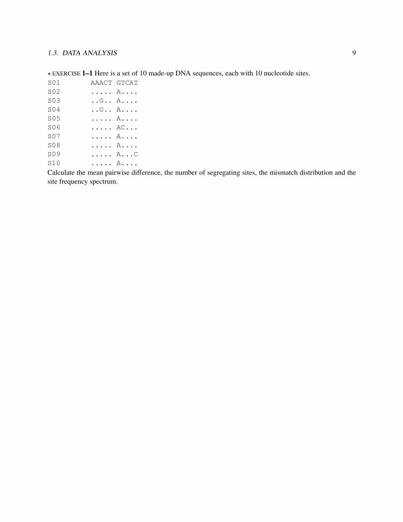
? EXERCISE 1–1 Here is a set of 10 made-up DNA sequences, each with 10 nucleotide sites.S01 AAACT GTCATS02 ..... A....S03 ..G.. A....S04 ..G.. A....S05 ..... A....S06 ..... AC...S07 ..... A....S08 ..... A....S09 ..... A...CS10 ..... A....
Calculate the mean pairwise difference, the number of segregating sites, the mismatch distribution and thesite frequency spectrum.

10 LECTURE 1. DESCRIPTIVE STATISTICS FOR DNA SEQUENCES
Lecture 2
The Method of Maximum Likelihood
Before doing this exercise, please read Using Likelihood, which you can find at http://www.anthro.utah.edu/˜rogers/pubs/index.html.
2.1 Maximum likelihood exercises with genetics problems
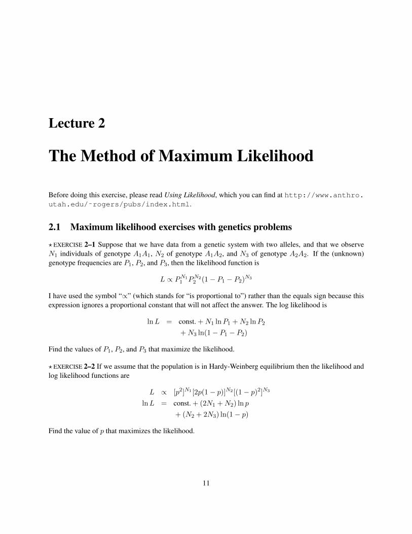
? EXERCISE 2–1 Suppose that we have data from a genetic system with two alleles, and that we observeN1 individuals of genotype A1A1, N2 of genotype A1A2, and N3 of genotype A2A2. If the (unknown)genotype frequencies are P1, P2, and P3, then the likelihood function is
L ∝ PN11 PN2
2 (1− P1 − P2)N3
I have used the symbol “∝” (which stands for “is proportional to”) rather than the equals sign because thisexpression ignores a proportional constant that will not affect the answer. The log likelihood is
lnL = const. +N1 lnP1 +N2 lnP2
+N3 ln(1− P1 − P2)
Find the values of P1, P2, and P3 that maximize the likelihood.
? EXERCISE 2–2 If we assume that the population is in Hardy-Weinberg equilibrium then the likelihood andlog likelihood functions are
L ∝ [p2]N1 [2p(1− p)]N2 [(1− p)2]N3
lnL = const. + (2N1 +N2) ln p
+ (N2 + 2N3) ln(1− p)
Find the value of p that maximizes the likelihood.
11

12 LECTURE 2. THE METHOD OF MAXIMUM LIKELIHOOD

Lecture 3
Genetic Drift
3.1 The four causes of evolutionary change
1. mutation
2. selection
3. migration (a.k.a. gene flow)
4. genetic drift
3.2 What is genetic drift?
• It is everything that is left over after you account for the effects of mutation, selection, and migration.
• It consists of all the stochastic (random) effects on allele frequencies. These include everything fromMendelian segregation to the risk of accidentally walking in front of a bus.
How can one possibly model such an ill-defined hodgepodge?
3.3 The Wright-Fisher model
The population does not vary in size. In each generation, it consists of N individuals, each produced by theunion of two randomly chosen gametes.
Generating gametes Each gamete is constructed by the following algorithm: (1) choose a parent at ran-dom from among the N individuals of the previous generation. (2) Choose a random half of that parent’sDNA. (Don’t worry about genetic linkage; we will be dealing here with one locus at a time.) If there are twoalleles A1 and A1, segregating at some locus, what is the probability that the gamete that we construct car-ries a copy of A1? If the parent was an A1A1 homozygote, then we are bound to get A1 in the gamete. If theparent was an A1A2 heterozygote, then the gamete has a 50% chance of carrying A1. Thus, the algorithm
13

14 LECTURE 3. GENETIC DRIFT
generates an A1-bearing gamete with probability p1 = P11 + P12/2, where P11 and P12 are the frequen-cies of genotypes A1A1 and A1A2 within the parental generation. Note that the formula for p1 is exactlythe same as the formula for the frequency of A1 among the parents. Conclusion: The Wright-Fisher algo-rithm for generating gametes is equivalent to drawing genes at random with replacement from the parentalpopulation. To clarify this idea, many authors have made use of the urn metaphor.
The urn metaphor In an urn full of balls, a fraction p of the balls are red and a fraction 1 − p are black.Each ball represents a gene. The red balls represent copies of one allele; the black ones copies of another.The fraction p represents the frequency of the red allele in the population. The urn will be used to produce anew generation in which there are N diploid individuals, or 2N genes. To produce the new generation, weperform the following operation 2N times: draw a random ball from the urn, write down its color, and thenreturn the ball to the urn. The number of red balls drawn represents the number of copies of the red allele inthe new generation, and similarly for the black balls. Both numbers are random variables. Their probabilitydistribution was taken by Wright and Fisher as a model of the process of genetic drift.
The Wright-Fisher model is undoubtedly simpler than reality, but it has been remarkably successful atdealing with the stochastic variation in real populations. Let us be content with it, at least for the moment,and ask about its properties. In the urn, the frequency of red balls is p. Let p′ denote the frequency of redballs among those drawn. The difference between p′ and p represents the effect of genetic drift. How largeis this difference likely to be?
If we repeated the urn experiment over and over, the average value of p′ would get closer and closer top. Another way to say this is to say that the expected value of p′ equals p. In notation,
E[p′] = p
where the symbol E represents the “expectation,” or average.But unless N is extremely large, there will be some difference between p′ and p, so we can write
p′ = p+ ε
Here, ε (the greek letter “epsilon”) represents the effect of genetic drift. Its expected value is 0, but itsvariance is1
V [ε] = E[ε2] =p(1− p)
2N
Genetic drift is important when this variance is large; unimportant when it is small. The formula capturestwo influences:
1. Drift is unimportant when p(1− p) is near 0. This happens when p ≈ 0 and also when p ≈ 1.
2. Drift is unimportant when N is very large.
3. Drift is most important when p ≈ 1/2 and N is small.
Show a plot of p against t.
1To see where this formula comes from, look up the binomial distribution in any text on probability and statistics.

3.4. CLASSICAL THEORY OF HOMOZYGOSITY AND HETEROZYGOSITY 15
Table 3.1: Average heterozygosity
Pop. Bl. grp.a Proteinb Classicalc RFLPd RSPe STR-4f STR-2g STR-3h
Africa 0.164 0.179 0.163 0.297 0.322 0.769 0.807 0.850Asia 0.145 0.164 0.189 0.327 0.377 0.681 0.685 0.820Europe 0.179 0.186 0.202 0.379 0.432 0.724 0.730 0.807
Note: Largest entry in each column is in boldface. Columns are in order of increasing European heterozygosity.a32 blood groups [22].b80 protein polymorphisms [22].c110 classical polymorphisms [1].d79 restriction fragment length polymorphisms [1].e30 RFLPs consisting solely of restriction site polymorphisms [13].f30 tetranucleotide STRs [13].g30 dinucleotide short tandem repeat polymorphisms (STRs). Difference between Africa and Europe is significant [1].h5 trinucleotide STRs [35].
3.4 Classical theory of homozygosity and heterozygosity
Let Jt represent the probability that two genes chosen at random from some population are copies of thesame allele. If the population mates at random, then J will also be the homozygosity. The gene diversity (orheterozygosity) is H = 1 − J . Several gene diversity estimates are shown in table 3.1. These statistics areaffected by several evolutionary forces:
1. Mutations reduce J because they are more likely to make identical genes less similar than to makedifferent genes identical.
2. Genetic drift tends to move allele frequencies toward 0 and 1. Consequently 2pq gets smaller, het-erozygosity declines, and homozygosity increases.
To measure the effects of these forces, we need a model. Let us begin with a model dealing only with thefirst force.
3.4.1 Drift only
Let Jt denote the probability that two genes drawn at random from the population of generation t are copiesof the same allele. There is a simple model that relates J in one generation to its value in the generationbefore:
Jt+1 =1
2N+
(1− 1
2N
)Jt
The first term on the right accounts for the possibility that the two genes in generation t+ 1 may be copiesof the same gene in generation t. Since there are 2N genes in the population, the two genes are copies ofthe same gene with probability 1/(2N) and are copies of distinct genes with probability 1− 1/(2N). In thelatter case, they are by definition copies of the same allele with probability Jt.
This model says that each generation’s value of J is a weighted average of 1 and the previous value ofJ . Consequently, J converges toward 1. We are eventually left with no heterozygotes at all.

16 LECTURE 3. GENETIC DRIFT
3.4.2 Drift plus mutation
To make the model interesting, we need to add in some other evolutionary force. Let us add in mutation. Theeasiest way to do this employs the model of “infinite alleles,” which assumes that every mutation producesan allele that has never existed before. Thus, two genes can be identical only if there has been no mutationalong the evolutionary path that connects them. In particular, there can have been no mutation during thepast generation in the path leading to either of our two genes. If u is the mutation rate per generation, then1 − u is the probability that no mutation occurs along a single evolutionary path during a generation, and(1− u)2 is the probability that neither of our two genes has mutated in the past generation. Thus,
Jt+1 = (1− u)2(
1
2N+
(1− 1
2N
)Jt
)Population geneticists are not very accurate people and tend to ignore whatever they can. Consider thefollowing:
u (1− u)2 1− 2u
0.00100 0.9980010000 0.998000.00010 0.9998000100 0.999800.00001 0.9999800001 0.99998
The smaller the value of u, the less the difference between (1 − u)2 and 1 − 2u. Since mutation rates arevery small numbers, population geneticists never trouble themselves about the difference between (1− u)2
and 1 − 2u. In the present case, 1 − 2u makes the algebra simpler. Similarly, if u is small and N is large,(1− 2u)/(2N) is hardly different from 1/(2N). Applying both simplifications gives
Jt+1 ≈1
2N+
(1− 2u− 1
2N
)Jt
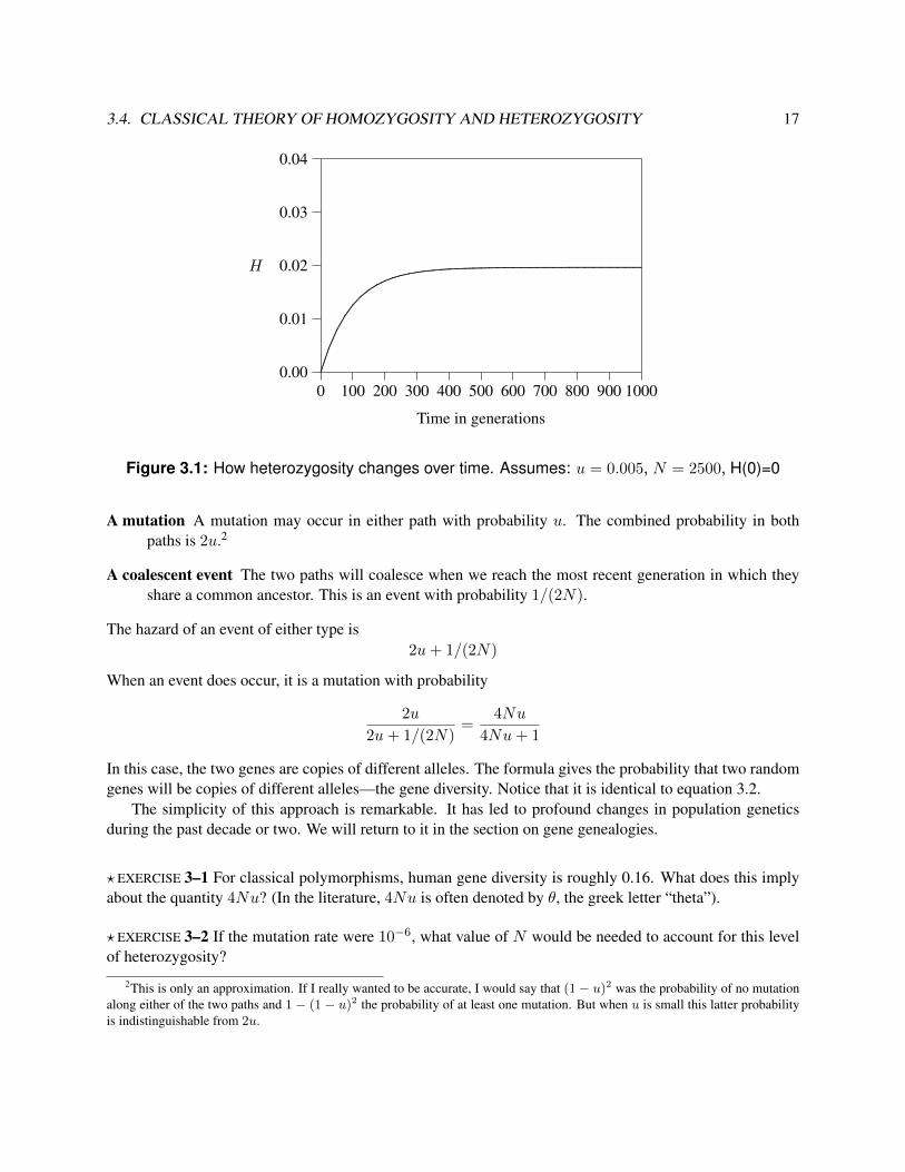
This equation doesn’t look very different from the one with drift only, but it leads to a very different conclu-sion. Rather than converging toward unity, this one levels out at a different equilibrium value, as shown infigure 3.1.
To find the equilibrium algebraically, set Jt+1 = Jt and solve the resulting equation. The result is
J =1
4Nu+ 1(3.1)
The gene diversity (or heterozygosity) is
H = 1− J =4Nu
4Nu+ 1(3.2)
3.4.3 A simpler way: coalescent theory
Take a random pair of genes and peer backwards down their ancestries. So long as the two evolutionarypaths remain distinct, two types of event may happen in any given generation:
3.4. CLASSICAL THEORY OF HOMOZYGOSITY AND HETEROZYGOSITY 17
0.00
0.01
0.02
0.03
0.04
H
0 100 200 300 400 500 600 700 800 900 1000
Time in generations
.................................................................................................................................................................................................................
.....................................................................................
....................................................................................................................................................................................................................................................................................................................................................................
Figure 3.1: How heterozygosity changes over time. Assumes: u = 0.005, N = 2500, H(0)=0
A mutation A mutation may occur in either path with probability u. The combined probability in bothpaths is 2u.2
A coalescent event The two paths will coalesce when we reach the most recent generation in which theyshare a common ancestor. This is an event with probability 1/(2N).
The hazard of an event of either type is2u+ 1/(2N)
When an event does occur, it is a mutation with probability
2u
2u+ 1/(2N)=
4Nu
4Nu+ 1
In this case, the two genes are copies of different alleles. The formula gives the probability that two randomgenes will be copies of different alleles—the gene diversity. Notice that it is identical to equation 3.2.
The simplicity of this approach is remarkable. It has led to profound changes in population geneticsduring the past decade or two. We will return to it in the section on gene genealogies.
? EXERCISE 3–1 For classical polymorphisms, human gene diversity is roughly 0.16. What does this implyabout the quantity 4Nu? (In the literature, 4Nu is often denoted by θ, the greek letter “theta”).
? EXERCISE 3–2 If the mutation rate were 10−6, what value of N would be needed to account for this levelof heterozygosity?
2This is only an approximation. If I really wanted to be accurate, I would say that (1 − u)2 was the probability of no mutationalong either of the two paths and 1 − (1 − u)2 the probability of at least one mutation. But when u is small this latter probabilityis indistinguishable from 2u.
18 LECTURE 3. GENETIC DRIFT
? EXERCISE 3–3 Using these same values for N and u, suppose that H were equal to 0.01 in generation 0.What would its value be in generation 20?
? EXERCISE 3–4 Using the same value for N , plot the variance of ε for values of p ranging from 0 through 1.
? EXERCISE 3–5 The square root of the variance is called the standard deviation and (in this case) providesan estimate of the magnitude of a typical value of ε. For what value of p is this standard deviation largest?How large is it at this value of p?
? EXERCISE 3–6 Figure 3.1 assumed that u = 0.005 and N = 2, 500. Under these assumptions, what is theequilibrium value of H? Is it consistent with the figure?

Lecture 4
Gene Genealogies
The coalescent process [12, 17] describes the ancestry of a sample of genes. As we trace the ancestry of eachmodern gene backwards from ancestor to ancestor, we occasionally encounter common ancestors—geneswhose descendants include more than one gene in the modern sample. Each time this happens, the numberof ancestors shrinks in size. Eventually, we reach the gene that is ancestral to the entire modern sample, andthe process ends.
Since the mid-1980s, this model has revolutionized our understanding of the effects of genetic drift andmutation. Many of the results obtained this way have been entirely new. Others have merely confirmedresults that were obtained long before. Either way, the coalescent model provides a method of studying driftand migration that is far easier than the methods that geneticists used to use. The material presented belowis not difficult, but you need to learn several mathematical tricks before you start. I will get these out of theway in the first section below.
4.1 Preliminaries
Trick 1 If the hazard of death is h per day, then the expected life-span is 1/h days.
For concreteness, suppose that we are talking about the life-span of a piece of kitchen glassware. Eventually,someone will drop it and it will break. Suppose that the hazard of breakage is h per day and its expectedlifespan is T days. Trick 1 tells us that T = 1/h.
We are envisioning time here as a continuous variable and assuming that the glass may break at anyinstant. It makes no sense to talk about the probability of breakage at a particular instant, because that hasto be zero. Instead, h is a probability density. (See Just Enough Probability.) Specifically, it is the densitythat the glass will break at a particular instant given that it has not broken already. This sort of density isoften called a hazard, and we are assuming that the hazard does not change. This implies that the lifespan(t) is a random variable whose probability distribution is exponential. The mean of this distribution is 1/h,as shown in appendix 4.B. In the exercise below, you will derive this formula for the case in which time isdiscrete.
? EXERCISE 4–1 Trick 1 refers to the case in which time is continuous, but the result also holds when timeis discrete. For example, suppose you are tossing a glass into the air and then catching it. On each toss,
19
20 LECTURE 4. GENE GENEALOGIES
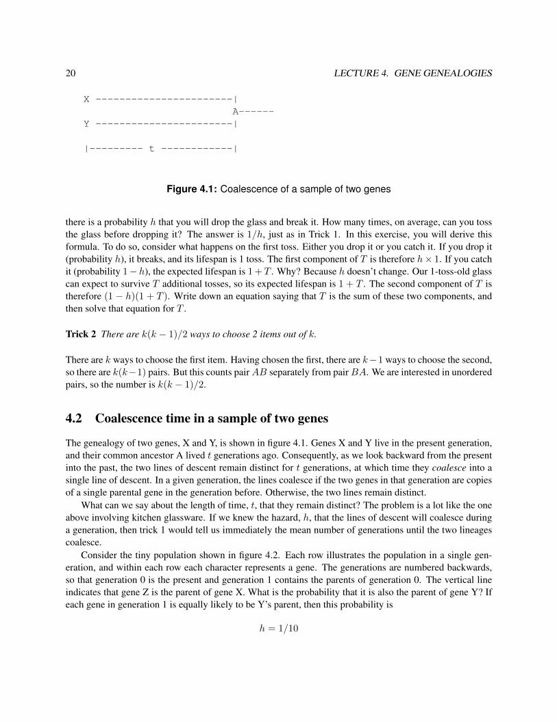
X -----------------------|A------
Y -----------------------|
|--------- t ------------|
Figure 4.1: Coalescence of a sample of two genes
there is a probability h that you will drop the glass and break it. How many times, on average, can you tossthe glass before dropping it? The answer is 1/h, just as in Trick 1. In this exercise, you will derive thisformula. To do so, consider what happens on the first toss. Either you drop it or you catch it. If you drop it(probability h), it breaks, and its lifespan is 1 toss. The first component of T is therefore h× 1. If you catchit (probability 1− h), the expected lifespan is 1 + T . Why? Because h doesn’t change. Our 1-toss-old glasscan expect to survive T additional tosses, so its expected lifespan is 1 + T . The second component of T istherefore (1 − h)(1 + T ). Write down an equation saying that T is the sum of these two components, andthen solve that equation for T .
Trick 2 There are k(k − 1)/2 ways to choose 2 items out of k.
There are k ways to choose the first item. Having chosen the first, there are k−1 ways to choose the second,so there are k(k−1) pairs. But this counts pairAB separately from pairBA. We are interested in unorderedpairs, so the number is k(k − 1)/2.
4.2 Coalescence time in a sample of two genes
The genealogy of two genes, X and Y, is shown in figure 4.1. Genes X and Y live in the present generation,and their common ancestor A lived t generations ago. Consequently, as we look backward from the presentinto the past, the two lines of descent remain distinct for t generations, at which time they coalesce into asingle line of descent. In a given generation, the lines coalesce if the two genes in that generation are copiesof a single parental gene in the generation before. Otherwise, the two lines remain distinct.
What can we say about the length of time, t, that they remain distinct? The problem is a lot like the oneabove involving kitchen glassware. If we knew the hazard, h, that the lines of descent will coalesce duringa generation, then trick 1 would tell us immediately the mean number of generations until the two lineagescoalesce.
Consider the tiny population shown in figure 4.2. Each row illustrates the population in a single gen-eration, and within each row each character represents a gene. The generations are numbered backwards,so that generation 0 is the present and generation 1 contains the parents of generation 0. The vertical lineindicates that gene Z is the parent of gene X. What is the probability that it is also the parent of gene Y? Ifeach gene in generation 1 is equally likely to be Y’s parent, then this probability is
h = 1/10

4.3. COALESCENCE TIMES IN A SAMPLE OF K GENES 21
________Population__________Generation 1: 0 Z 0 0 0 0 0 0 0 0
|Generation 0: 0 X 0 Y 0 0 0 0 0 0
Figure 4.2: A sample of two genes (X and Y) in a population of size 10. Gene Z is the parent ofgene X.
since there are 10 genes in generation 1. This answer would be the same no matter which gene in genera-tion 1 had been X’s parent.
Trick 1 immediately tells us that the mean coalescence time is 10 generations. Of course, 10 is reallythe number of genes in the population. If there are 2N genes in the population, then
h = 1/2N (4.1)
Now the answer becomes somewhat more interesting. The average pair of genes last shared a commonancestor 2N generations ago. This provides a connection between population size and the genealogy ofgenes. As we shall see in lecture 5, this connection lets us use genetics to study the history of populationsize.
In equation 4.1, the symbol N is a little confusing. If we are talking about an autosomal locus, thenthere are two genes for every person and N is the number of people in the population. The meaning of N isdifferent, however, if we are talking about a mitochondrial locus. In that case, the gene is transmitted onlythrough women, and locus is effectively haploid. Consequently, the number (2N) of genes is the number offemales in the population, and the symbol N represents half the number of females.• EXAMPLE 4–1Suppose that we somehow knew that the average pair of mitochondrial genes last shared a common an-cestor 100,000 years ago. What would this imply about population size? (Ignore the issue of statisticalerror.)◦ANSWER100,000 years is about 4000 generations, so the assumption implies that
2N = 4000
Since we are talking about a mitochondrial gene, this is really the number of women. If there are as manymen as women, then the population would contain 8000 individuals. This is about the size of a large villageor a very small town.
4.3 Coalescence times in a sample of K genes
Now consider a sample of K genes. (Figure 4.3 shows the case in which K = 4.) As we move backwardsin time from the present, the first coalescent event that we encounter reduces our sample from K to K − 1,the second from K − 1 to K − 2, and so on. After K − 1 coalescent events, only a single lineage is leftand no further coalescent events can occur. There are thus K − 1 intervals to consider. The first (i.e. themost recent) interval is the one in which there are K lines of descent. This interval is tK generations. Thenext interval has K − 1 lines of descent and is tK−1 generations long. The last interval is the one with two
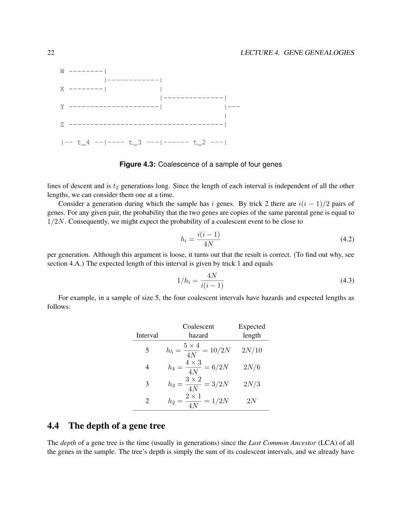
22 LECTURE 4. GENE GENEALOGIES
W --------||------------|
X --------| ||--------------|
Y ---------------------| |---|
Z ------------------------------------|
|-- t_4 --|---- t_3 ---|------ t_2 ---|
Figure 4.3: Coalescence of a sample of four genes
lines of descent and is t2 generations long. Since the length of each interval is independent of all the otherlengths, we can consider them one at a time.
Consider a generation during which the sample has i genes. By trick 2 there are i(i − 1)/2 pairs ofgenes. For any given pair, the probability that the two genes are copies of the same parental gene is equal to1/2N . Consequently, we might expect the probability of a coalescent event to be close to
hi =i(i− 1)
4N(4.2)
per generation. Although this argument is loose, it turns out that the result is correct. (To find out why, seesection 4.A.) The expected length of this interval is given by trick 1 and equals
1/hi =4N
i(i− 1)(4.3)
For example, in a sample of size 5, the four coalescent intervals have hazards and expected lengths asfollows:
Coalescent ExpectedInterval hazard length
5 h5 =5× 4
4N= 10/2N 2N/10
4 h4 =4× 3
4N= 6/2N 2N/6
3 h3 =3× 2
4N= 3/2N 2N/3
2 h2 =2× 1
4N= 1/2N 2N
4.4 The depth of a gene tree
The depth of a gene tree is the time (usually in generations) since the Last Common Ancestor (LCA) of allthe genes in the sample. The tree’s depth is simply the sum of its coalescent intervals, and we already have
4.4. THE DEPTH OF A GENE TREE 23
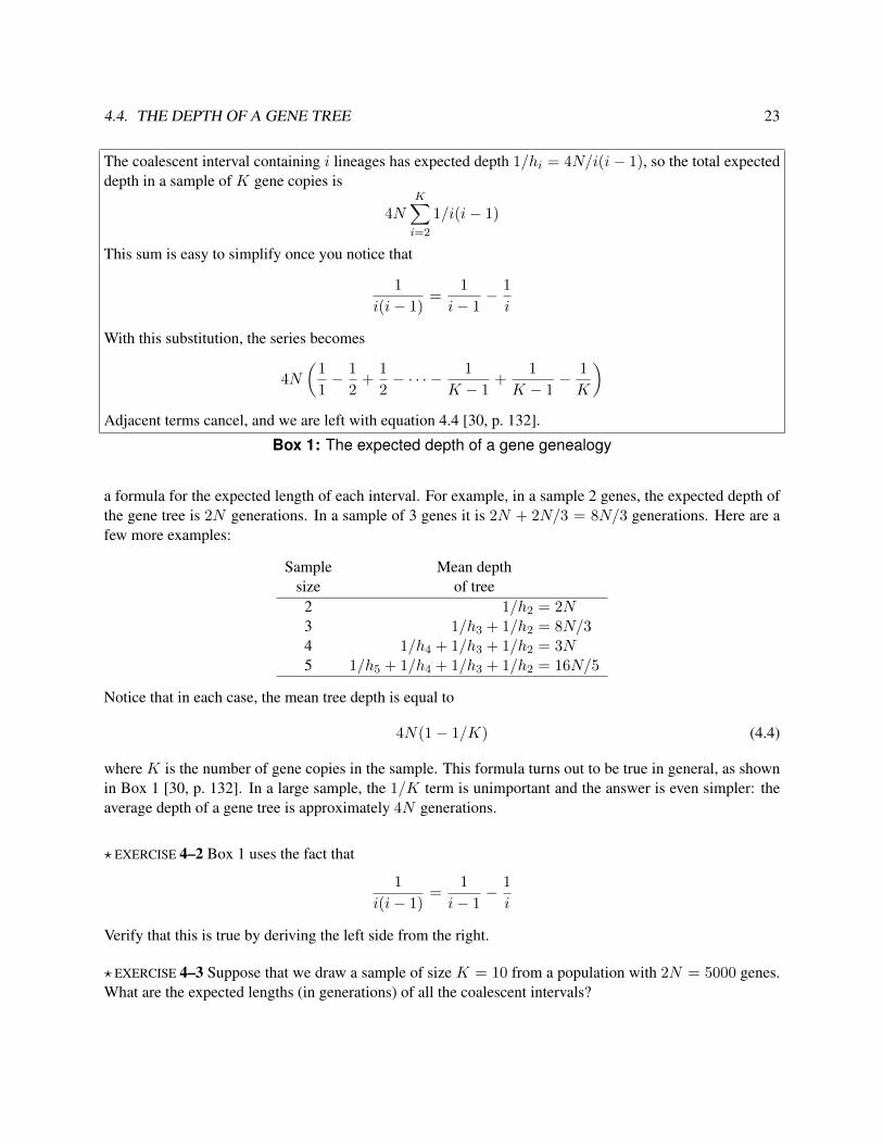
The coalescent interval containing i lineages has expected depth 1/hi = 4N/i(i− 1), so the total expecteddepth in a sample of K gene copies is
4NK∑i=2
1/i(i− 1)
This sum is easy to simplify once you notice that
1
i(i− 1)=
1
i− 1− 1
i
With this substitution, the series becomes
4N
(1
1− 1
2+
1
2− · · · − 1
K − 1+
1
K − 1− 1
K
)Adjacent terms cancel, and we are left with equation 4.4 [30, p. 132].
Box 1: The expected depth of a gene genealogy
a formula for the expected length of each interval. For example, in a sample 2 genes, the expected depth ofthe gene tree is 2N generations. In a sample of 3 genes it is 2N + 2N/3 = 8N/3 generations. Here are afew more examples:
Sample Mean depthsize of tree
2 1/h2 = 2N3 1/h3 + 1/h2 = 8N/34 1/h4 + 1/h3 + 1/h2 = 3N5 1/h5 + 1/h4 + 1/h3 + 1/h2 = 16N/5
Notice that in each case, the mean tree depth is equal to
4N(1− 1/K) (4.4)
where K is the number of gene copies in the sample. This formula turns out to be true in general, as shownin Box 1 [30, p. 132]. In a large sample, the 1/K term is unimportant and the answer is even simpler: theaverage depth of a gene tree is approximately 4N generations.
? EXERCISE 4–2 Box 1 uses the fact that
1
i(i− 1)=
1
i− 1− 1
i
Verify that this is true by deriving the left side from the right.
? EXERCISE 4–3 Suppose that we draw a sample of size K = 10 from a population with 2N = 5000 genes.What are the expected lengths (in generations) of all the coalescent intervals?

24 LECTURE 4. GENE GENEALOGIES
-||--|-| |
|---|---|| |
|| |---| |---|
| |--------| |-------------------------------------------|
| |------------| |
|------| |
| |---| |-------| |
|--| | |------| |------| |
| | |-| | | ||------------| | |-| | |
| |-------------| |----------------------------------|
| |-| |-| ||-----------| | |-| | |
| || | ||---| |-----|| | |
|-| |----| | |
| |-| |--------||| |-|| |
|---|--|
Figure 4.4: Coalescence of a sample of twenty genes

4.A. A MORE DETAILED TREATMENT (OPTIONAL) 25
? EXERCISE 4–4 In a sample of 10,000 genes, what is the expected age of the LCA? What fraction of thisage is accounted for by the interval during which the tree contained only two lineages?
When the sample is large, K(K−1)/2 is a large number. Consequently, initial coalescent intervals tendto be short. In a sample of size 20, the most recent coalescent interval is (on average) 0.5 percent as long asthe interval that ends with the root. Figure 4.4 shows an example. Note the short terminal branches and thedeep basal branch.
4.A A more detailed treatment (optional)
4.A.1 Preliminaries
Before explaining the formula for the general case—that of a coalescent interval during which the samplehas K genes—we need one additional mathematical trick.
Trick 3 The sum of the numbers from 1 through k is k(k + 1)/2.
This trick was supposedly discovered by Carl Friedrich Gauss (one of the greatest mathematicians of alltime) when he was just six years old. According to the story, Gauss’s teacher gave the class an assignmentto keep it busy while he graded papers: Sum the numbers from 1 through 100. Two minutes later, Gausswalked to the front of the room with his answer. The answer was correct, but Gauss was punished for failingto do the work the hard way. Here is how he did it.
First he wrote down1 + 2 + · · ·+ 99 + 100
Then, being bored and discouraged, he wrote it out backwards just below:
1 + 2 + · · · + 99 + 100100 + 99 + · · · + 2 + 1
Then the insight struck—he noticed that each of the columns added to 101:
1 + 2 + · · · + 99 + 100100 + 99 + · · · + 2 + 1
101 + 101 + · · · + 101 + 101
Since there are 100 columns, the sum of all the numbers here is 100 × 101. And this is twice the sum thathe was looking for. Thus,
1 + 2 + · · ·+ 99 + 100 =100× 101
2
In the general case,
1 + 2 + · · ·+ k =k(k + 1)
2
Trick 4 ex is approximately 1 + x when x is small.
Here ex is the exponential function, and is also written as exp(x). You can verify the trick with a calculator.

26 LECTURE 4. GENE GENEALOGIES
X --------------------|B---------------|
Y --------------------| |A---
Z ------------------------------------|
|--------- t_3 -------|------ t_2 ----|
Figure 4.5: Coalescence of a sample of three genes
4.A.2 Coalescence times in an interval with three genes
Figure 4.5 shows the genealogy of a sample of three genes. It has two coalescent events, one at node A (theroot) and another at node B. The time between the present and the root can be broken into two intervals oflength t2 and t3, where t2 is the number of generations during which the genealogy has two lines of descentand t3 is the number of generations during which it had three. What can we say about the lengths of theseintervals?
The first point to notice is that the intervals are independent. As we ponder the length of one interval,we need not worry about the length of the other. The second point to notice is that we already know themean of t2. The preceding section showed that the mean coalescence time for a sample of two genes is 2Ngenerations.
This leaves us with only one question to answer: What is the mean time until the first coalescent event ina sample of three genes? We could answer this question using trick 1 if we knew the hazard of a coalescentevent in a sample of that size. Let us therefore consider the probability that a coalescent event occurs duringsome given generation.
It is easier to calculate first the probability of the event that all three lines of descent remain distinct.This requires that
1. X and Y are copies of different parental genes. We already know that this event has probability1− 1/2N .
2. Z is neither a copy of X’s parent nor a copy of Y’s parent. This event has probability (2N − 2)/2N .(Of the 2N genes that we can choose between, 2 produce a coalescent event and 2N −2 do not.) Thisprobability can also be written as 1− 1/N .
Thus, the probability that no coalescent event occurs in some particular generation is equal to
1− h = (1− 1/2N)(1− 1/N)
Now it is time to invoke trick 4. If the population is large, then 2N will be a large number and 1/2N and1/N will both be small. Trick 4 thus allows the probability above to be re-expressed as
1− h ≈ e−1/2Ne−1/N = e−3/2N
4.A. A MORE DETAILED TREATMENT (OPTIONAL) 27
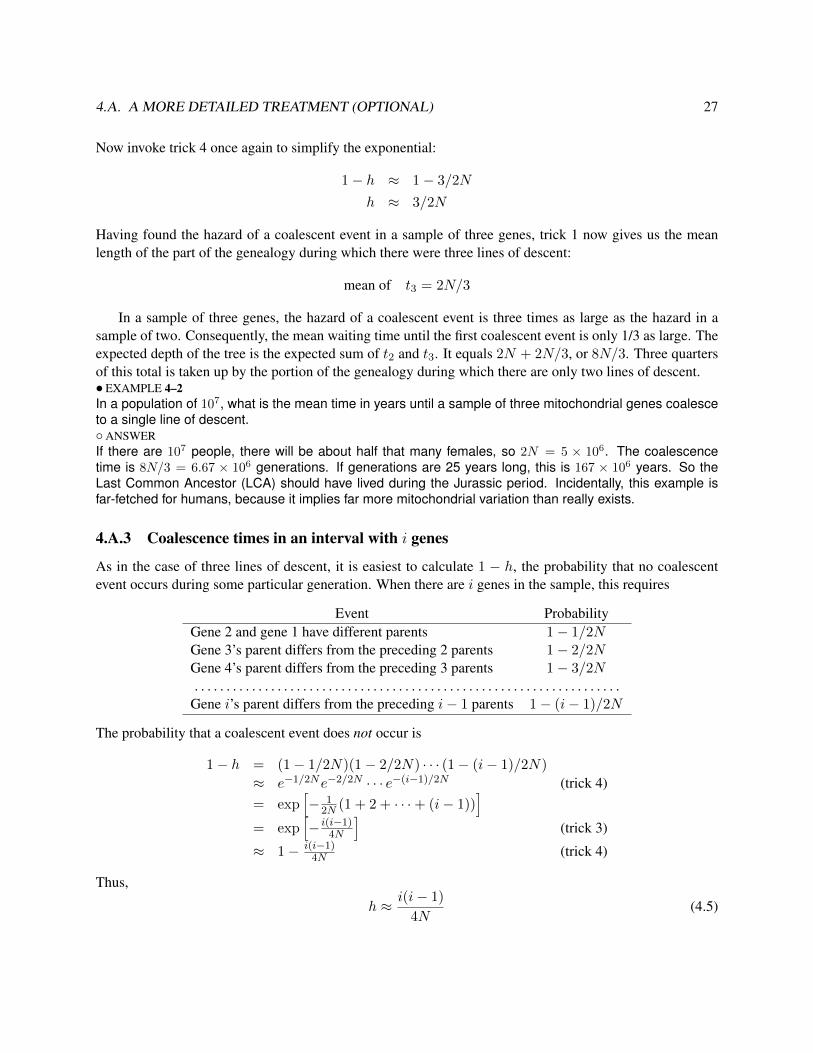
Now invoke trick 4 once again to simplify the exponential:
1− h ≈ 1− 3/2N
h ≈ 3/2N
Having found the hazard of a coalescent event in a sample of three genes, trick 1 now gives us the meanlength of the part of the genealogy during which there were three lines of descent:
mean of t3 = 2N/3
In a sample of three genes, the hazard of a coalescent event is three times as large as the hazard in asample of two. Consequently, the mean waiting time until the first coalescent event is only 1/3 as large. Theexpected depth of the tree is the expected sum of t2 and t3. It equals 2N + 2N/3, or 8N/3. Three quartersof this total is taken up by the portion of the genealogy during which there are only two lines of descent.• EXAMPLE 4–2In a population of 107, what is the mean time in years until a sample of three mitochondrial genes coalesceto a single line of descent.◦ANSWERIf there are 107 people, there will be about half that many females, so 2N = 5 × 10⁶. The coalescencetime is 8N/3 = 6.67 × 10⁶ generations. If generations are 25 years long, this is 167 × 106 years. So theLast Common Ancestor (LCA) should have lived during the Jurassic period. Incidentally, this example isfar-fetched for humans, because it implies far more mitochondrial variation than really exists.
4.A.3 Coalescence times in an interval with i genes
As in the case of three lines of descent, it is easiest to calculate 1 − h, the probability that no coalescentevent occurs during some particular generation. When there are i genes in the sample, this requires
Event ProbabilityGene 2 and gene 1 have different parents 1− 1/2NGene 3’s parent differs from the preceding 2 parents 1− 2/2NGene 4’s parent differs from the preceding 3 parents 1− 3/2N. . . . . . . . . . . . . . . . . . . . . . . . . . . . . . . . . . . . . . . . . . . . . . . . . . . . . . . . . . . . . . . . . . .
Gene i’s parent differs from the preceding i− 1 parents 1− (i− 1)/2N
The probability that a coalescent event does not occur is
1− h = (1− 1/2N)(1− 2/2N) · · · (1− (i− 1)/2N)
≈ e−1/2Ne−2/2N · · · e−(i−1)/2N (trick 4)= exp
[− 1
2N (1 + 2 + · · ·+ (i− 1))]
= exp[− i(i−1)
4N
](trick 3)
≈ 1− i(i−1)4N (trick 4)
Thus,
h ≈ i(i− 1)
4N(4.5)
28 LECTURE 4. GENE GENEALOGIES
4.B The mean of an exponential random variable (optional)
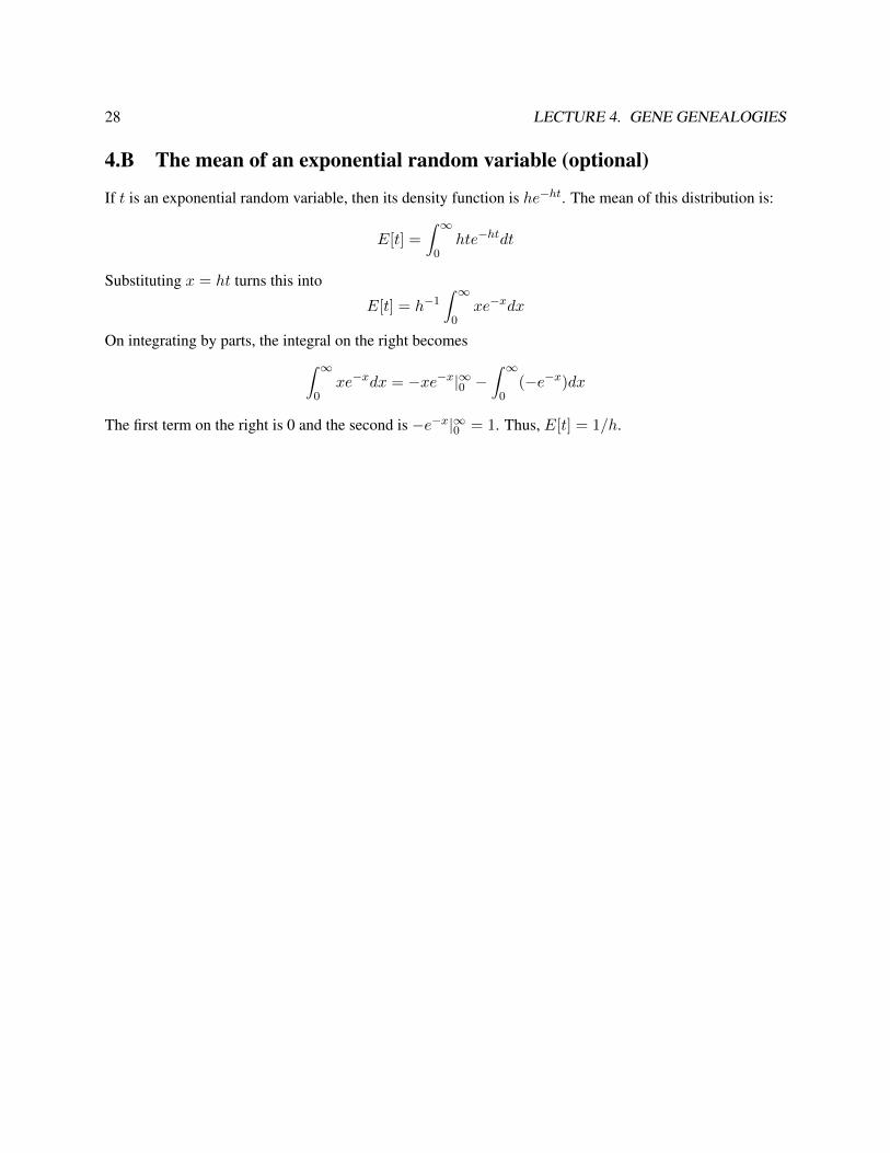
If t is an exponential random variable, then its density function is he−ht. The mean of this distribution is:
E[t] =
∫ ∞0
hte−htdt
Substituting x = ht turns this into
E[t] = h−1∫ ∞0
xe−xdx
On integrating by parts, the integral on the right becomes∫ ∞0
xe−xdx = −xe−x|∞0 −∫ ∞0
(−e−x)dx
The first term on the right is 0 and the second is −e−x|∞0 = 1. Thus, E[t] = 1/h.
Lecture 5
Relating Gene Genealogies to Genetics
This course began with a section on probability theory. Then came material on genetic variation and geneticdrift. In the last lecture, we discussed gene genealogies. These may have seemed like disconnected threads.This lecture will tie them all together.
We will make extensive use of the theory introduced last time about genealogical relationships amonggenes. Although that theory is elegant, it is also limited, for gene genealogies cannot be observed. Theydescribe obscure events that happened many thousands of years ago. We can never know the genealogyof a sample of genes. We can estimate it from genetic data, but that requires a theory that relates genegenealogies to observable genetic data.
This lecture begins by adding mutations to gene genealogies, and then relates these to two genetic statis-tics: the number S of segregating sites, and the mean pairwise difference π between nucleotide sequences.Finally, it will consider two ways to estimate the parameter θ.
5.1 The number of mutations on a gene genealogy
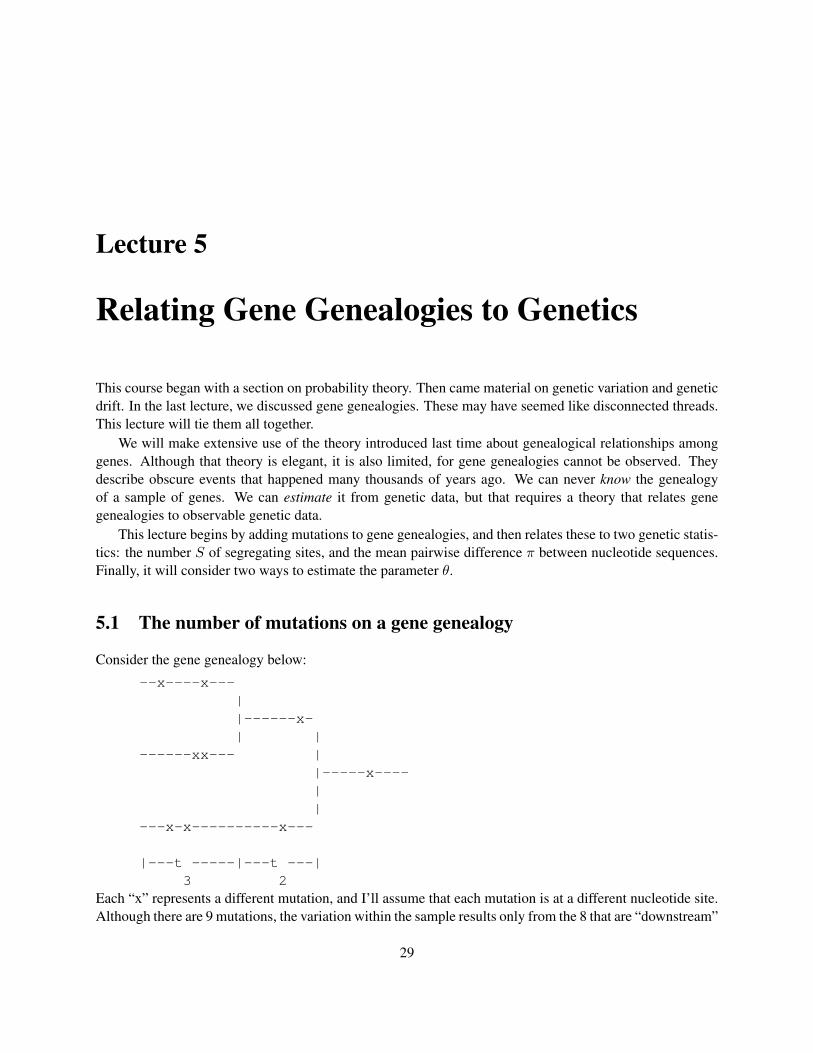
Consider the gene genealogy below:
--x----x---||------x-| |
------xx--- ||-----x----||
---x-x----------x---
|---t -----|---t ---|3 2
Each “x” represents a different mutation, and I’ll assume that each mutation is at a different nucleotide site.Although there are 9 mutations, the variation within the sample results only from the 8 that are “downstream”
29
30 LECTURE 5. RELATING GENE GENEALOGIES TO GENETICS
of the genealogy’s root. The 9th mutation would produce an identical effect on all members of the sampleand is therefore of no interest to us. For our purposes, this is a genealogy with 8 mutations.
How many mutations would we expect to see in a sample of 3 genes? The answer will depend in parton the number of nucleotide sites being examined. We expect more mutations per generation on an entirechromosome than at a single nucleotide site. Although this effect is large, we can avoid dealing with itdirectly by using a flexible definition of the mutation rate, u. If we are studying a single nucleotide site,then u will represent the expected number of mutations per generation per site. If we are studying a largerregion—say an entire gene or chromosome—then u will represent the expected number of mutations pergeneration in this entire region.
Unless we are studying a large genomic region, u will be very small and can be interpreted not only asthe expected number of mutations per generation, but also as the probability of a single mutation. This isbecause we don’t lose much, when mutations are very rare, by ignoring the remote possibility that severalof them happen at once.
The expected number of mutations depends not only on the mutation rate, u, but also on the total lengthof the gene genealogy. In a sample of 3 genes, this length is
L = 3t3 + 2t2 (5.1)
where t3 is the length of the coalescent interval during which the genealogy had 3 lines of descent, and t2is the length of the other interval. If there are u mutations per generation, then we would expect this tree tohave uL mutations—if we knew the value of L.
But since the value of L is ordinarily unknown,
E[# of mutations] = E[uL] = uE[L]
To calculate this expected value, we need the expectation ofL. The direct approach would involve inspectingthousands of gene genealogies, each generated by the coalescent process described in the last lecture. Youcannot, of course, look at even one real gene genealogy, let alone thousands of them. You could write acomputer program to simulate the process, but we can do the same job more easily using the theory fromthe previous lecture.
The E stands for “expectation,” and in the present context it refers to an average over genealogies. Forexample,E[t2] is the expectation (that is, average) of t2 over a very large number of genealogies. We learnedin the last lecture that E[t2] = 2N and E[t3] = 2N/3. Thus, equation 5.1 implies that the expectation of Lis
E[L] = 3E[t3] + 2E[t2] = 2N + 4N
In general, the expected length of the coalescent interval during which there are i lines of descent is (seeequation 4.3)
E[ti] =4N
i(i− 1)
and the contribution of this interval to the expected length (including all branches) of the tree is
iE[ti] =4N
i− 1
5.2. THE MODEL OF INFINITE SITES 31
The total expected length of the tree is
E[L] =K∑i=2
iE[ti] = 4NK−1∑i=1
1
i(5.2)
where K is the number of genes in the sample. The expected number of mutations on the gene genealogy isthus
E[# of mutations] = uE[L]
= 4NuK−1∑i=1
1
i
= θK−1∑i=1
1
i(5.3)
where u is the mutation rate per generation, and θ = 4Nu, a quantity that appears often in the formulas ofpopulation genetics. It equals twice the number of mutations that occur each generation in the populationas a whole. Like u its magnitude depends on the size of the genomic region under study (see p. 30). Below,we will consider the problem of estimating θ from genetic data.
5.2 The model of infinite sites
We can now calculate the expected number of mutations in a gene genealogy of any size. The next chal-lenge is to connect this result to data—to genetic differences between individuals. The easiest approachinvolves what is known as the “model of infinite sites.” This model assumes mutation never strikes the samenucleotide site twice. This model is never really correct, but it is often a good approximation, especially inintra-specific data sets where the genetic differences between individuals are small. It makes sense to use itwhen the mutation rate per nucleotide site is low enough that only a small fraction of nucleotide sites willmutate twice in any given gene genealogy.
This model, of course, is only an approximation. In the real world, nucleotide sites may mutate morethan once. Appendix section 5.B (p. 36) shows that these violations occur, on average, at a fraction (ut)2/2of sites, where u is the mutation rate per site per generation and t is the number of generations.
For example, suppose that some branch of the gene genealogy is t = 104 generations long and thatu = 10−8. Along this branch, the expected number of mutations at a single nucleotide site is ut = 10−4. Inan entire human genome, the number of sites is about 3× 10⁹. The expected number of sites that violate theinfinite sites model is therefore
3× 109 × 10−8/2 = 15
The model of infinite sites is expected to fail only at 15 sites out of 3 billion. This analysis should notbe taken too literally, because the mutation rate is not really constant across the genome, and we may beinterested in much longer time intervals. Nonetheless, it does show that the model of infinite sites workswell when the product ut is small.
32 LECTURE 5. RELATING GENE GENEALOGIES TO GENETICS
5.3 The number of segregating sites
If mutation never strikes the same site twice, then the number S of segregating (i.e. polymorphic) sites in adata set is the same as the number of mutations in its gene genealogy, as given in equation 5.3. The expectednumber of segregating sites is [37]
E[S] = θ{1 + 1/2 + 1/3 + · · ·+ 1/(K − 1)} (5.4)
Finally, we have arrived at a statistic that can be calculated from data. The expected number of segregatingsites is equal to θ times some number that increases with sample size. Thus, we expect more segregatingsites in a large sample. But the effect of sample size is not pronounced, because the sum in the expressionabove doesn’t increase very fast. Here are a few example values:
K∑K−1i=1 1/i
2 1.003 1.505 2.08
10 2.82100 5.17
1000 7.48
In a sample of 100, we expect only about 5 times as many segregating sites as in a sample of 2.The effect of the population size, on the other hand, is pronounced since E[S] is proportional to θ, and θ
is proportional to the population’s size. In a population twice as large, we expect twice as many segregatingsites.
5.4 The mean pairwise difference
Given any pair of DNA sequences, it is a simple matter to count the number of nucleotide positions at whichthey differ. Given a sample of size K, there areK(K−1)/2 pairwise comparisons that can be made and wecan count the number of nucleotide differences between each pair. Averaging these numbers gives a statisticthat is called the “mean pairwise nucleotide difference” and is generally denoted by the symbol π.1
What is the expected value of π? The number of nucleotide site differences between a pair of sequencesis the same as the number of segregating sites in a sample of size 2. Thus, equation 5.4 tells us that theaverage pair of sequences differs at θ sites. Averaging over all the pairs in a sample doesn’t change thisexpectation, so
E[π] = θ (5.5)
This gives us the expected value of a second statistic that can be estimated from genetic data, and thistime the formula is especially simple. As in the case of S, we can expect the value of π to be large if thepopulation is large, small if the population is small.
1Some authors [20] use the capital letter (Π) to denote the mean pairwise differences per sequence and the lower-case letter (π)to refer to the mean pairwise difference per site. I use the lower-case letter for both purposes.
5.5. THETA AND TWO WAYS TO ESTIMATE IT 33
? EXERCISE 5–1 Just above, I said that if the expected difference between each pair of sequences is θ, thenthe expectation of π is also θ. Prove that this is so.
? EXERCISE 5–2 For the following questions, assume that the population mates at random, has constant size2N = 1000, that there is no selection, and that the mutation rate is u = 1/2000 per sequence per generation.Assume that you are working with a sample of K = 5 DNA sequences, and that mutations obey the modelof infinite sites.
1. What is the expected depth of the gene tree? (In other words, the expected number of generationssince the last common ancestor.)
2. What is the expected length of the tree? (In other words, the expected sum of the lengths of allbranches in the tree.)
3. What is the expected number of mutations on the tree?
4. What is the expected number of mutational differences between each pair of sequences?
5.5 Theta and Two Ways to Estimate It
In this lecture, we have twice run into the parameter θ, which is proportional to the product of mutation rateand population size. This parameter appears often in population genetics, and it is useful to have a way toestimate it. The results above suggest two ways. Equation 5.4 suggests
θS =S∑K−1i=1
1i
(5.6)
and equation 5.5 suggests.θπ = π (5.7)
Here θ is read “theta hat.” The “hat” indicates that these formulas are intended to estimate the parameter θ.To make sure that these formulas estimate the same parameter, it is important to be consistent. S usually
refers to the number of segregating sites within some larger DNA sequence. To make π comparable, weinterpret it here as the mean pairwise difference per sequence rather than that per site. We also need tointerpret u as the mutation rate per sequence when we define θ = 4Nu.
With these consistent definitions, θS and θπ estimate the same parameter. It seems natural to suppose thattheir values would be similar in real data. Let’s have a look at some human mitochondrial DNA sequencedata.
5.6 Example
Jorde et al (ref) published sequence data from the control region of human mitochondrial DNA. The ex-ample described here uses 430 nucleotide positions from HVS1 (the first hypervariable region). Jorde etal sequenced DNAs from all three major human racial groups, but this example will deal only with the 77Asian and 72 African sequences. In these data:

34 LECTURE 5. RELATING GENE GENEALOGIES TO GENETICS
Asian AfricanS 82 63∑K−1i=1 1/i 4.915 4.847
θS (per sequence) 16.685 12.998π (per sequence) 6.231 9.208
To compare statistics referring to sequences of different lengths, it is often convenient to divide by thenumber of sites, which produces:
Asian AfricanθS (per site) 0.039 0.030π (per site ) 0.014 0.021
The pattern is unchanged here because both data sets have the same number of sites.The theory above says that π and θS are both estimates of the parameter θ, so we have every reason to
expect their values to be similar. Yet θS is half again as large as π in the African data and nearly three timesas large in the Asian. Why are these numbers so different?
There are at least four possibilities worth considering:
Sampling error To figure out whether these discrepancies are large enough to worry about, we need atheory of errors.
Natural selection The theory we have used assumes neutral evolution. If selection has been at work, thenwe have no reason to think that π and θS will be equal. In fact, the difference between π and θSis often used to test the hypothesis of selective neutrality. (Look up Tajima’s D in any textbook onpopulation genetics.)
Variation in population size Our theory also assumes that the population has been constant in size. Weneed to investigate how π and θS respond to changes in population size.
Failure of the infinite sites model Our theory assumes that mutation never strikes the same site twice.
5.7 The probability that a nucleotide site is polymorphic within a sample
In comparisons between pairs of haploid human genomes, about one nucleotide site in a thousand is poly-morphic. In larger samples, of course, the polymorphic fraction is larger. What is the fraction (QK) thatis expected to be polymorphic in a sample of size K? It is easier to work with the monomorphic fraction,1 − QK . The gene genealogy is monomorphic only if no mutation occur in any coalescent interval. Letus consider first the coalescent interval during which there were k ancestors. As we trace time backwardsacross this interval, we might encounter either of two types of event: a mutation or a coalescent event. Weencounter a coalescent event first if (and only if) the interval is free of mutations.
During this interval, coalescent events happen with hazard λ2 = k(k − 1)/4N per generation, andmutations happen with hazard λ1 = ku, where u is the mutation rate per site per generation. Once an eventdoes occur, it is a coalescent event with probability
zk =λ2
λ1 + λ2= 1− θ
θ + k − 1
5.A. SAMPLING ERROR IN π AND S (OPTIONAL) 35
where θ = 4Nu [see reference 33, pp. 48–49]. This is the probability that the kth coalescent interval is freeof mutations. When θ is small, zk is approximately
zk ≈ 1− θ
k − 1≈ e−θ/(k−1)
Because the mutations that occur in different coalescent intervals are independent, these probabilities mul-tiply. The entire gene genealogy is free of mutations with probability
1−QK = z2z3z4 · · · zK≈ exp[−θ{1 + 1/2 + 1/3 + ...+ 1/(K − 1)}] (5.8)
The expected fraction of polymorphic sites is QK . For example, if θ = 1/1000, the fraction of polymorphicsites should be 0.001 in a sample of size 2, 0.003 in a sample of 10, and 0.005 in a sample of 100. Thepolymorphic fraction increases with K, but not very fast.
5.A Sampling error in π and S (optional)
If π and S are calculated from a sample of K sequences drawn at random from a randomly-mating popula-tion, their sampling variances are
V [π] = θK + 1
3(K − 1)+ θ2
2(K2 +K + 3)
9K(K − 1)[28, p. 449] (5.9)
V [S] = θK−1∑i=1
1
i+ θ2
K−1∑i=1
1
i2(5.10)
V [θS ] = θ1∑K−1
i=11i
+ θ2∑K−1i=1
1i2(∑K−1
i=11i
)2 (5.11)
To find the standard errors of π, S, and θS are the square roots of these variances.To apply these formulas, we need to know the value of θ, but this we do not know—all we have are
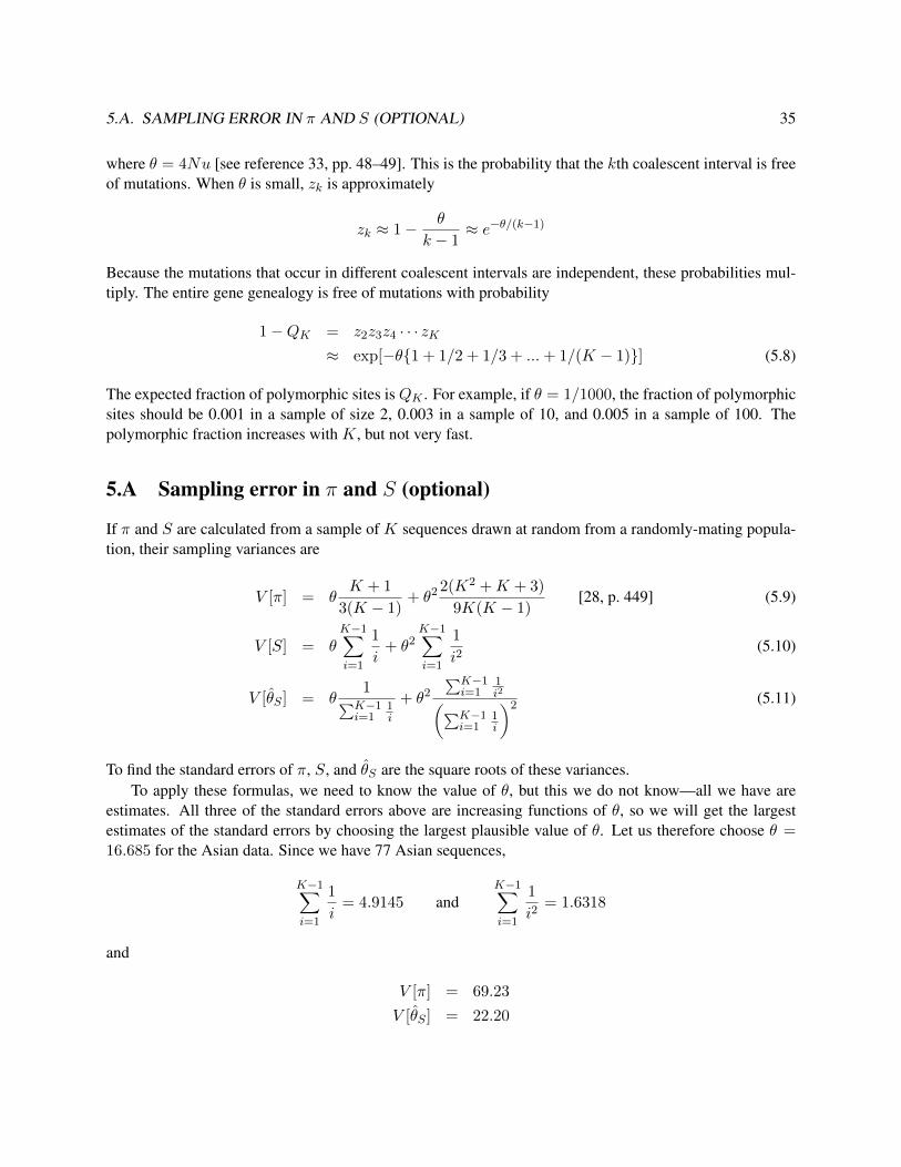
estimates. All three of the standard errors above are increasing functions of θ, so we will get the largestestimates of the standard errors by choosing the largest plausible value of θ. Let us therefore choose θ =16.685 for the Asian data. Since we have 77 Asian sequences,
K−1∑i=1
1
i= 4.9145 and
K−1∑i=1
1
i2= 1.6318
and
V [π] = 69.23
V [θS ] = 22.20

36 LECTURE 5. RELATING GENE GENEALOGIES TO GENETICS
The standard errors are the square roots of these numbers:
S.E.[π] = 8.23
S.E.[θS ] = 4.71
If our estimates were independent and normally distributed, π would provide a confidence interval with anupper bound equal to
6.231 + 1.96× S.E.[π] = 22.59
The estimate of θS would provide a confidence interval with a lower bound equal to
16.685− 1.96× S.E.[π] = 7.4
Since the two confidence intervals overlap, we cannot reject (at the 0.05 significance level) the hypothesisthe two estimates reflect the same underlying value of θ.
But there is every reason to be skeptical of this analysis: There is no reason to think that the samplingdistributions of these statistics are normal and even less to think that they are independent. (After all, theyare calculated from the same data.) So this approach is hard to defend.
The alternative approach is to use the coalescent principle to generate simulated data sets on a computer.The joint sampling distribution of π and θS can be estimated from the simulated data.
5.B When you assume the model of infinite sites, how wrong are you likelyto be? (optional)
The model of infinite sites assumes that mutation never strikes the same site twice. Clearly, this is only anapproximation, and when we use this model we are bound to introduce errors. The question is, how large arethese errors likely to be? What fraction of the sites in our data can be expected to mutate more than once?
To find out, let us consider the mutations that occur at some nucleotide site along a single branch of agene genealogy. If the branch is t generations long, then the number,X , of mutations is a Poisson-distributedrandom variable with mean λ = ut, where u is the mutation rate per generation.
Consider the probability, P , that X < 2. This is the probability that our site conforms to the model ofinfinite sites. Because X is Poisson,
P = e−λ + λe−λ
If λ is small, e−λ ≈ 1 − λ + λ2/2, ignoring terms of order λ3. (This is from the series expansion of theexponential function.) To this standard of approximation,
P ≈ 1− λ+ λ2/2
+ λ− λ2 + λ3/2
≈ 1− λ2/2
The fraction of sites that violate the infinite sites model is approximately 1 − P = λ2/2—a very smallnumber.

Lecture 6
The Site Frequency Spectrum
6.1 The empirical site frequency spectrum
In a sample of K genes, a polymorphic site can divide the sample into 1 mutant and K − 1 non-mutants,into 2 mutants and K − 2 non-mutants, and so on. There may be at most K − 1 copies of the mutant if thesite is to be polymorphic. In many cases we can’t tell which allele is the mutant, so category i gets conflatedwith category K − i. Such spectra are called “folded.” I will call a site a “singleton” if the mutant is presentin a single copy, a “doubleton” if it is present in two copies, and so on.
6.1.1 An unfolded spectrum
Consider the set of DNA sequence data below:
123456HumanSequence1 AATAGCHumanSequence2 ..AC..HumanSequence3 .TACT.HumanSequence4 ..ACT.---------------------ChimpSequence1 AAAATCChimpSequence2 AAAATC
There are 4 human sequences and 2 chimpanzee sequences. There are 6 sites of which 4 are polymorphic(segregating) within the human sample. We calculate the empirical spectrum by considering the sites one ata time.
Site 1 is fixed and therefore does not contribute to the spectrum.
Site 2 has both an A and a T within the human sample but has only an A within the chimpanzee sample.The odds are that the ancestor of humans and chimps had an A at this site, so we can infer that T isthe mutant allele. Since there is only one copy of T in the human sample, site 2 is a singleton. So far,our spectrum looks like this:
37
38 LECTURE 6. THE SITE FREQUENCY SPECTRUM
Singletons : 1Doubletons :Tripletons :
Site 3 is like site 2. The human sample has a T and 3 As, and the chimp sample has only As. We infer thatT is the mutant allele and count this site as another singleton. The spectrum now looks like this:
Singletons : 2Doubletons :Tripletons :
Site 4 has an A and 3 Cs, but it appears that A was the ancestral allele. We count this site as a tripleton, sothe spectrum becomes
Singletons : 2Doubletons :Tripletons : 1
Site 5 has 2 Gs and 2 Ts. It does not matter which of these is ancestral. Either way, the site is a doubleton.The spectrum becomes
Singletons : 2Doubletons : 1Tripletons : 1
Site 6 does not contribute to the spectrum.
We are done. The empirical spectrum has 2 singletons, 1 doubleton, and 1 tripleton.
6.1.2 A folded spectrum
In the preceding section, the chimpanzee sequences were used at each site to infer which nucleotide wasancestral and which was the mutant. Let us now pretend that we have no chimpanzee sequences and thereforecannot tell the the ancestral allele from the mutant. Instead of counting mutants, we will count the rarest(sometimes called the minor) allele at each site. This time, however, I will omit the invariant sites (1 and 6),which do not contribute to the spectrum.
Site 2 The rare allele, T, is present in a single copy, so this site contributes to the singleton category just asit did for the unfolded spectrum.
Site 3 Ditto: another singleton
Site 4 The rare allele, A, is present in a single copy, so this site is a singleton. Recall that it was a tripletonin the unfolded spectrum.
Site 5 A doubleton

6.2. THE EXPECTED SPECTRUM UNDER NEUTRALITY AND CONSTANT POPULATION SIZE39
The folded spectrum looks like this:
Singletons : 3Doubletons : 1
The only difference is that site 4, which was a tripleton in the unfolded spectrum, becomes a singleton in thefolded spectrum.
In general, the ith category of the folded spectrum contains not only category i of the unfolded spectrum,but also category K − i, where K is the number of DNA sequences in the sample.
6.2 The expected spectrum under neutrality and constant population size
This section deals with the special case of selective neutrality and constant population size. I will assumeinitially that we can tell mutants from ancestral alleles so that our spectrum will be unfolded.
6.2.1 A site’s position in the spectrum depends on its position in the gene tree
Consider the following gene tree:
----A------||----B---| |
----------- ||-----------||
------C-------------
Mutations A and C are singletons, whereas B is a doubleton. A mutation that occurs in the most recentcoalescent interval can only be a singleton. One that occurs in the next most recent interval can be either asingleton or a doubleton. One in the interval before that can be a singleton, a doubleton, or a tripleton. Andso on.

40 LECTURE 6. THE SITE FREQUENCY SPECTRUM
6.2.2 A tree with two leaves has nothing but singletons
To get a sense of how the process works, it helps to start with a tree with just two leaves:
-------------------|||-----------||
-------------------
|- 2N generations --|
Since the hazard is 1/2N , the mean depth of this tree is 2N generations and the total length is 4N . Weexpect 4Nu = θ mutations, all of which will be singletons.
6.2.3 A tree with three leaves has (on average) the same number of singletons and half thatnumber of doubletons
Now consider a tree with three leaves:---------
||--------------------| |
--------- ||--------||
------------------------------
|--2N/3--|-------- 2N --------|
Generations
If we could look at the spectrum just before the most recent coalescent event, it would look just like that ofthe tree with two leaves: θ singletons and no doubletons. At the time of the coalescent event, half of thesemutations (the ones on the upper branch) become doubletons. There is no further change in the number ofdoubletons, so the expected number of doubletons in a 3-leaf gene tree is θ/2. (We don’t need to worrythat mutation will turn any of our doubletons back into singletons because, under the infinite sites model,mutation never strikes the same site twice.)
We start this latest coalescent interval with θ/2 singletons, but then more singletons are added because ofnew mutations. How many new mutations should we expect to see? The interval’s expected length is 2N/3generations (see section 4.3), and it contains 3 lines of descent, so the sum of the branch lengths within thisinterval is (on average) 2N generations. We therefore expect 2Nu = θ/2 new singleton mutations.

6.3. HUMAN SITE FREQUENCY SPECTRA 41
The number of singletons that is added is precisely equal to the number that was lost. Thus, the newspectrum has θ singletons and θ/2 doubletons.
6.2.4 The theoretical spectrum for an arbitrary number of leaves
The argument that I used above gets progressively more tedious as leaves are added. It is better to use adifferent argument. I will skip the details here, but the results look like this [6]:
Sample Theoretical spectrumsize (singletons, doubletons, . . .)
2 θ3 θ, θ/24 θ, θ/2, θ/35 θ, θ/2, θ/3, θ/4
Etcetera
It is remarkable that as we increase sample size, the number of mutants in each category doesn’t change.We merely add a new category at the right side of the spectrum.
To use the theoretical formula with data, we need to substitute some estimate of θ. We might use themean pairwise difference, π, or the estimator
θS =S∑K−1i=1
1i
where K is the number of DNA sequences in the sample. Either of these estimators might work, since bothof them estimate θ under the stationary neutral model (see the discussion of equation 5.6 on page 33). Tochoose between these estimators, we need some additional criterion.
The sum of the observed spectrum is equal to the number S of segregating sites. It would be useful ifthe theoretical spectrum summed to the same value. This turns out to be so only if θS is used to estimate θ.
6.2.5 Folded theoretical spectra
When the spectrum is folded, we cannot distinguish category i from category K − i. Consequently, theexpected number in category i in the folded spectrum is the sum θ/i and θ/(K − i), the expected numbersin the two corresponding categories in the unfolded spectrum.
This works so long as i and K − i are not the same number. If they are the same number, then theexpected spectrum is simply θ/i.
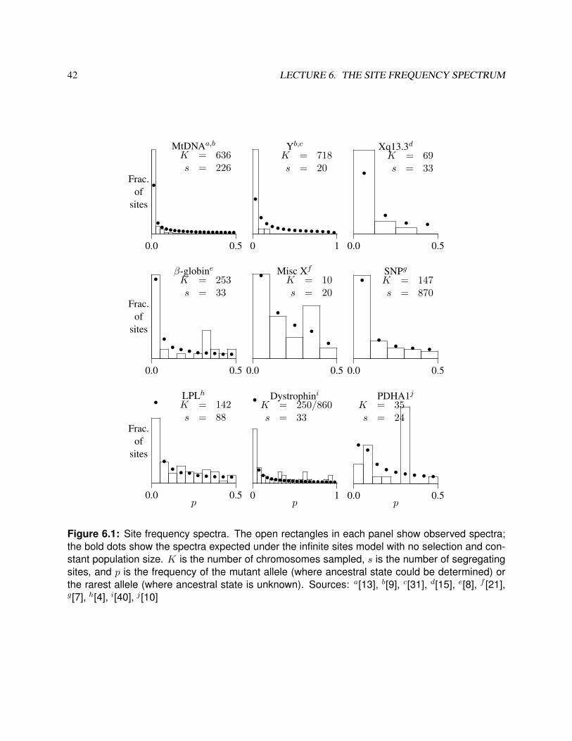
6.3 Human site frequency spectra
Figure 6.1 shows all of the human site frequency spectra that I was able to cull from the literature in the year2000. In each plot, the empirical spectrum is shown as a histogram, and the expected values under neutralevolution with constant population size are shown as bold dots. The top row shows three systems in whichthere is an excess of singletons, compared with the stationary neutral model. The middle row shows threesystems that seem to fit the neutral model, and the bottom row shows three systems in which there is a deficitof singletons and an excess of sites at intermediate frequency.
42 LECTURE 6. THE SITE FREQUENCY SPECTRUM
Frac.of
sites
0.0 0.5
MtDNAa,b
K = 636s = 226
•
•••••••••••••••••••
0 1
Yb,c
K = 718s = 20
•
••• • •• • •• • •• • •
0.0 0.5
Xq13.3dK = 69s = 33•
•• •
Frac.of
sites
0.0 0.5
β-globineK = 253s = 33
•
•• • • • • • • •
0.0 0.5
Misc Xf
K = 10s = 20
•
••
••
0.0 0.5
SNPgK = 147s = 870
•
•• • •
Frac.of
sites
0.0 0.5p
K = 142s = 88
LPLh•
•• • • • • • • •
0 1p
K = 250/860s = 33
Dystrophini•
•••••••••••••••••••
0.0 0.5p
PDHA1jK = 35s = 24
• •• • • • • • •
Figure 6.1: Site frequency spectra. The open rectangles in each panel show observed spectra;the bold dots show the spectra expected under the infinite sites model with no selection and con-stant population size. K is the number of chromosomes sampled, s is the number of segregatingsites, and p is the frequency of the mutant allele (where ancestral state could be determined) orthe rarest allele (where ancestral state is unknown). Sources: a[13], b[9], c[31], d[15], e[8], f [21],g[7], h[4], i[40], j [10]
6.4. EXERCISES 43
6.4 Exercises
? EXERCISE 6–1 For this exercise, use the toy data set in section 1.1, on p. 5. (1) Use S to estimate θ,(2) from this value, calculate the number of sites expected in each frequency category, (3) fold the resultingtheoretical spectrum by summing values for i andK− i. (4) Compare the result with the empirical spectrumthat we calculated earlier, in section 1.3.3.

44 LECTURE 6. THE SITE FREQUENCY SPECTRUM
Lecture 7
The Mismatch Distribution
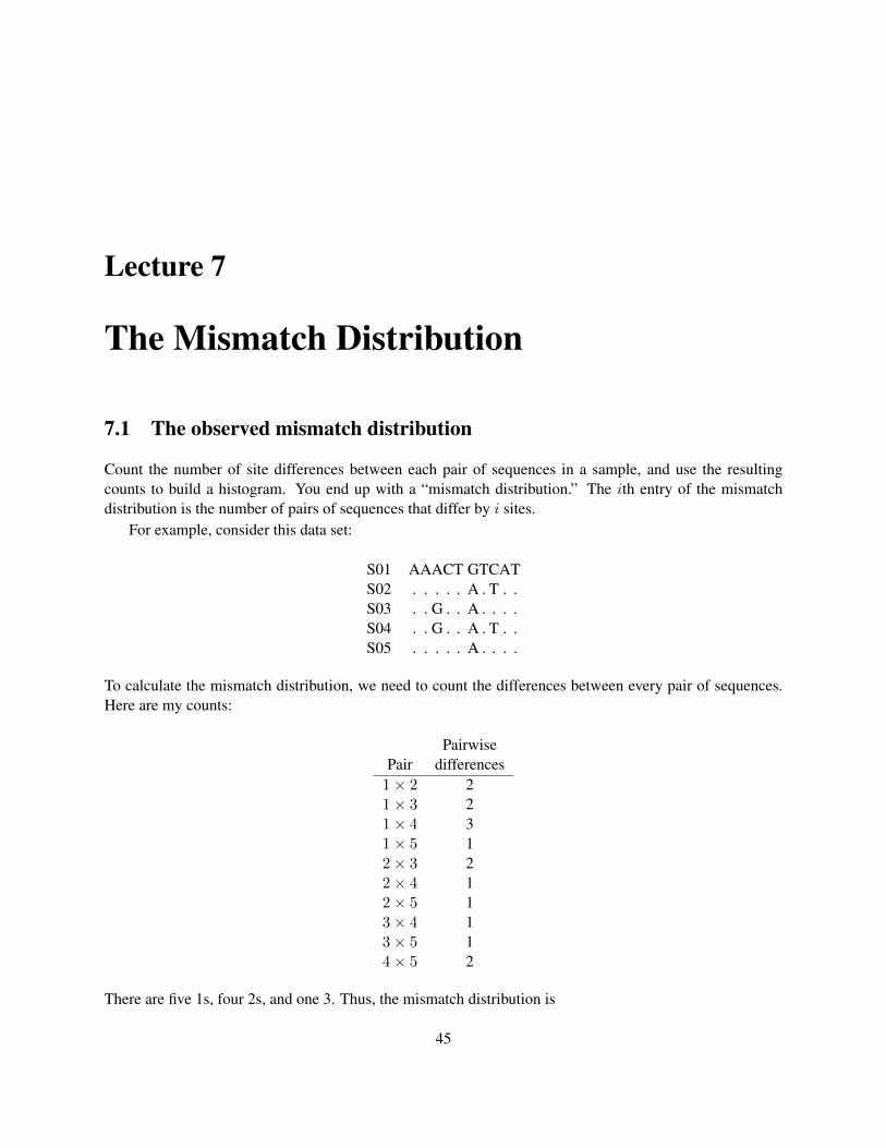
7.1 The observed mismatch distribution
Count the number of site differences between each pair of sequences in a sample, and use the resultingcounts to build a histogram. You end up with a “mismatch distribution.” The ith entry of the mismatchdistribution is the number of pairs of sequences that differ by i sites.
For example, consider this data set:
S01 AAACT GTCATS02 . . . . . A . T . .S03 . . G . . A . . . .S04 . . G . . A . T . .S05 . . . . . A . . . .
To calculate the mismatch distribution, we need to count the differences between every pair of sequences.Here are my counts:
PairwisePair differences
1× 2 21× 3 21× 4 31× 5 12× 3 22× 4 12× 5 13× 4 13× 5 14× 5 2
There are five 1s, four 2s, and one 3. Thus, the mismatch distribution is
45
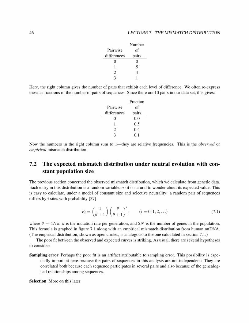
46 LECTURE 7. THE MISMATCH DISTRIBUTION
NumberPairwise of
differences pairs0 01 52 43 1
Here, the right column gives the number of pairs that exhibit each level of difference. We often re-expressthese as fractions of the number of pairs of sequences. Since there are 10 pairs in our data set, this gives:
FractionPairwise of
differences pairs0 0.01 0.52 0.43 0.1
Now the numbers in the right column sum to 1—they are relative frequencies. This is the observed orempirical mismatch distribution.
7.2 The expected mismatch distribution under neutral evolution with con-stant population size
The previous section concerned the observed mismatch distribution, which we calculate from genetic data.Each entry in this distribution is a random variable, so it is natural to wonder about its expected value. Thisis easy to calculate, under a model of constant size and selective neutrality: a random pair of sequencesdiffers by i sites with probability [37]
Fi =
(1
θ + 1
)(θ
θ + 1
)i, (i = 0, 1, 2, . . .) (7.1)
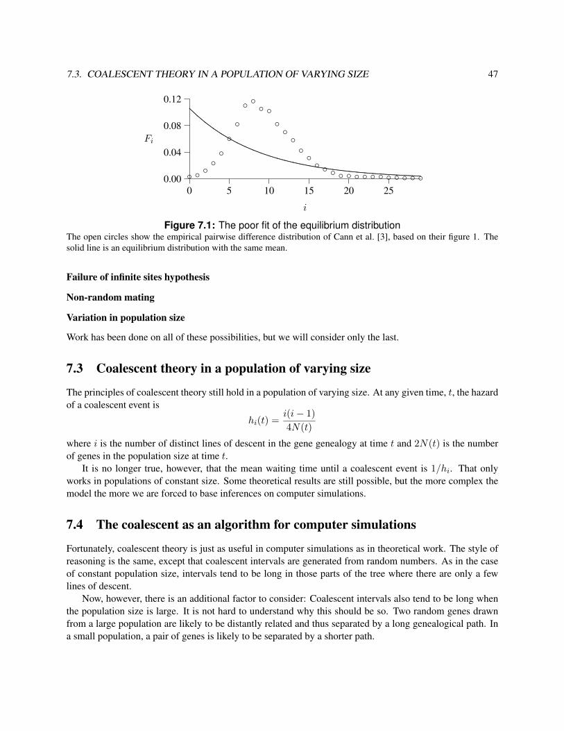
where θ = 4Nu, u is the mutation rate per generation, and 2N is the number of genes in the population.This formula is graphed in figure 7.1 along with an empirical mismatch distribution from human mtDNA.(The empirical distribution, shown as open circles, is analogous to the one calculated in section 7.1.)
The poor fit between the observed and expected curves is striking. As usual, there are several hypothesesto consider:
Sampling error Perhaps the poor fit is an artifact attributable to sampling error. This possibility is espe-cially important here because the pairs of sequences in this analysis are not independent: They arecorrelated both because each sequence participates in several pairs and also because of the genealog-ical relationships among sequences.
Selection More on this later
7.3. COALESCENT THEORY IN A POPULATION OF VARYING SIZE 47
0.00
0.04
0.08
0.12
Fi
0 5 10 15 20 25
i
◦ ◦ ◦◦◦◦◦
◦ ◦ ◦ ◦◦◦◦◦◦◦ ◦ ◦ ◦ ◦ ◦ ◦ ◦ ◦ ◦ ◦ ◦ ◦ ◦
.............................................................................................................................................................................................................................................................................................................................................................................................................................................................................................................................................................................................................................................................................................................
Figure 7.1: The poor fit of the equilibrium distributionThe open circles show the empirical pairwise difference distribution of Cann et al. [3], based on their figure 1. Thesolid line is an equilibrium distribution with the same mean.
Failure of infinite sites hypothesis
Non-random mating
Variation in population size
Work has been done on all of these possibilities, but we will consider only the last.
7.3 Coalescent theory in a population of varying size
The principles of coalescent theory still hold in a population of varying size. At any given time, t, the hazardof a coalescent event is
hi(t) =i(i− 1)
4N(t)
where i is the number of distinct lines of descent in the gene genealogy at time t and 2N(t) is the numberof genes in the population size at time t.
It is no longer true, however, that the mean waiting time until a coalescent event is 1/hi. That onlyworks in populations of constant size. Some theoretical results are still possible, but the more complex themodel the more we are forced to base inferences on computer simulations.
7.4 The coalescent as an algorithm for computer simulations
Fortunately, coalescent theory is just as useful in computer simulations as in theoretical work. The style ofreasoning is the same, except that coalescent intervals are generated from random numbers. As in the caseof constant population size, intervals tend to be long in those parts of the tree where there are only a fewlines of descent.
Now, however, there is an additional factor to consider: Coalescent intervals also tend to be long whenthe population size is large. It is not hard to understand why this should be so. Two random genes drawnfrom a large population are likely to be distantly related and thus separated by a long genealogical path. Ina small population, a pair of genes is likely to be separated by a shorter path.

48 LECTURE 7. THE MISMATCH DISTRIBUTION
Table 7.1: Hypothetical two-epoch population history
2Ni tiEpoch (genes) (generations)
0 106 20001 104 ∞
Computer simulations are most useful if they deal with only a few parameters at a time. Thus, we needsome economical way to describe the history of a population that changes in size.
7.5 Stepwise models of population history
Population growth is ordinarily regulated by density-dependent mechanisms that allow small populations togrow and cause large ones to shrink. Consequently, most biologists think that the sizes of most populationsare roughly constant most of the time. Now and then, something happens to disturb this equilibrium, and thepopulation either grows or shrinks until a new equilibrium is attained. Over a long time scale, the periodsof change would look like relatively sudden changes in the size of a population that was otherwise roughlyconstant.
This is the conventional view of demographic history, and it motivates the stepwise model of popu-lation history that is used here. I will assume that history can be divided into a series of epochs duringwhich the population does not change. Epochs are separated by episodes of rapid change, which I treat asinstantaneous. They are numbered backwards from the most recent (epoch 0) to the most ancient.1
Table 7.1 shows the parameters of a hypothetical population history with two epochs. The table describesa population that was small (10,000 people) early in time, grew suddenly 2000 generations ago, and has beenlarge (1,000,000 people) ever since. The history of this hypothetical population is graphed in figure 7.2.
With genetic data is it not possible to estimate Ni and ti directly. We can, however, estimate the related
1Rogers and Harpending [25] numbered them in the opposite direction.
N0
N1
0 tTime before present, measured in generations
Population Size.....................................................................................................................................................................................................................................................................................................................................................................................................................................................................................................................................................................................................................................................................................................................................................
Figure 7.2: At t generations before the present, the population expands from female size N1 tofemale size N0. The model’s 3 parameters are θ0 ≡ 2uN0, θ1 ≡ 2uN1, and τ ≡ 2ut, where u is theaggregate mutation rate over all sites.

7.6. SIMULATIONS OF STATIONARY POPULATIONS 49
Table 7.2: Alternate parameterization of the same population history
Epoch θi τi
0 2000 41 20 ∞
parameters
θi = 4Niu (7.2)
τi = 2uti (7.3)
where u is the mutation rate. θi measures the size of the population during epoch i in units of 1/(2u) genes;τi measures the length of this epoch in units of 1/(2u) generations. The population history of table 7.1 canbe re-expressed in terms of θ and τ by multiplying each parameter by 2u. For example, if the mutation rateis 0.001 (per sequence per generation), then we obtain table 7.2.
7.6 Simulations of stationary populations
Figures 7.3–7.6, on pages 50–53, each show a simulation of a population with constant size. In each figure,the upper panel shows the time path of population size, which is simply a horizontal line in these first fourfigures. Proceding down each page, you will find the gene genealogy, the mismatch distribution and thespectrum. The expected mismatch distribution is shown as a solid line; the expected spectrum is shown as aseries of filled circles. In both cases, the expected values refer to a model of neutral evolution in a populationof constant size.
These figures make use of what I will call the “mutational time scale.” A unit of mutational time is theamount of time it takes, on average, for one mutation to accumulate along the genealogical path separatingtwo sequences. Thus, if two sequences have been separate for 5 units of mutational time, we expect them todiffer at about 5 nucleotide sites. Each unit of mutational time is equal to 1/(2u) generations.• EXAMPLE 7–1In human mitochondrial D-loop sequence, it has been estimated that the mutation rate is 4.1 × 10⁻⁶ pernucleotide per generation [34]. In the Jorde et al HVSI data there are 430 nucleotides, so u = 430 × 4.1 ×10−6 = 0.0018 per generation. Each unit of mutational time is 1/(2u) = 278 generations, which wouldcorrespond roughly to 6950 years.
Notice that neither the mismatch distributions nor the spectra of these equilibrium populations look muchlike the theoretical formulas would predict. Far from showing the smooth decline seen in the theoreticalcurves, the simulated mismatch distributions tend to be ragged, with multiple peaks. The site frequencyspectra also exhibit pronounced departures from their expected values. In order to get answers that look likethe theory, we would need to run the simulations many times and average the results. This is bad news, sincein real data analysis we cannot rewind the evolutionary process and look at it again and again. The situationis not hopeless, but it is clear that merely inspecting graphs such as these is not going to give us dependableanswers. We are going to need more sophisticated statistical methods.

50 LECTURE 7. THE MISMATCH DISTRIBUTION
Populationsize
0 9 18 27Mutational time before present
Genegenealogy
Mutational time before present
••••
• • ••
• •• •
•••• •••
••
•••
• •••• • •• • • ••
Mismatchdistribution
0 9 18 27Pairwise differences
◦
◦
◦
◦
◦ ◦ ◦
◦◦ ◦ ◦ ◦ ◦ ◦ ◦ ◦ ◦ ◦ ◦ ◦
◦ ◦
◦
◦
◦
◦◦
..............................................................................................................................................................................................................................................................................................................................................................................................................................................................................................................................................................................................................................................................................................................................................
Sitefrequencyspectrum
0 1/2Frequency of minor allele
•
•• • • • • • • • • • • • • • • • • • • • • • •
Figure 7.3: An equilibrium population with θ = 7
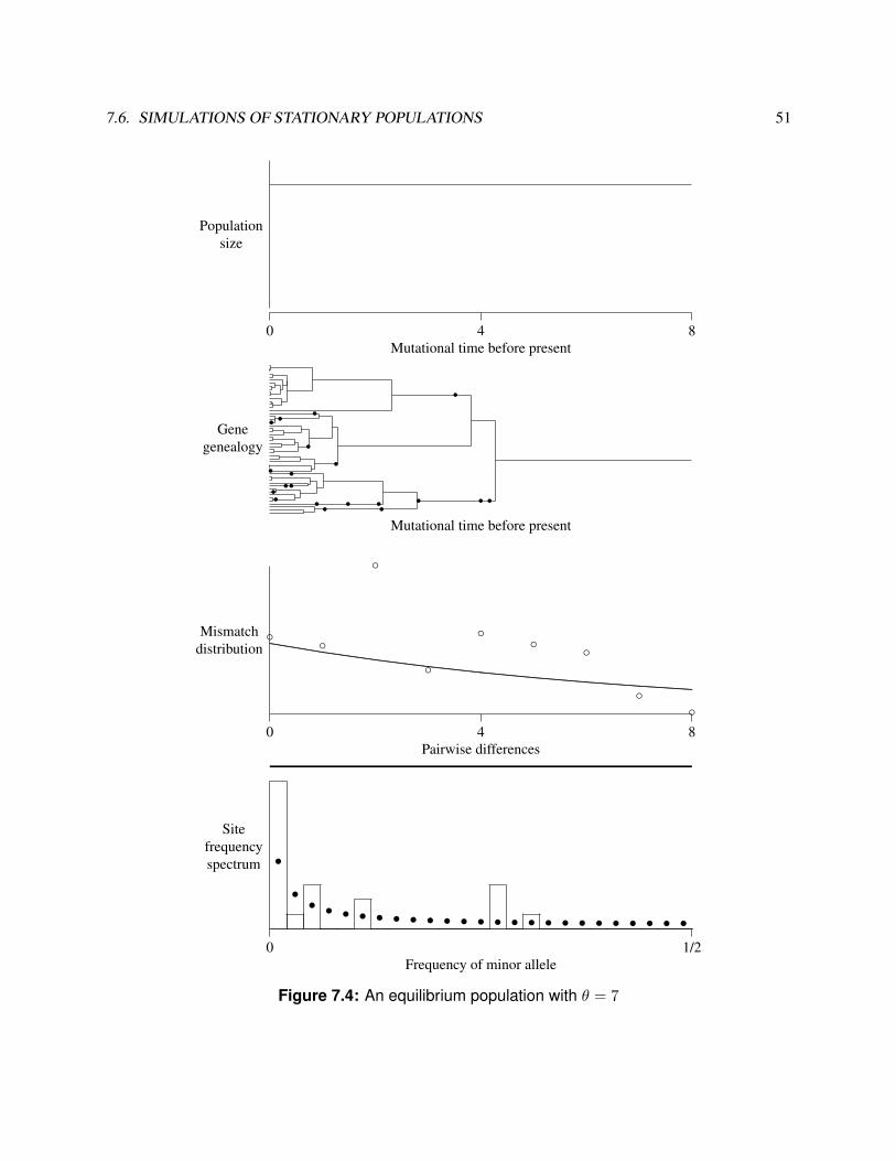
7.6. SIMULATIONS OF STATIONARY POPULATIONS 51
Populationsize
0 4 8Mutational time before present
Genegenealogy
Mutational time before present••• •••
••••
•• •
••
•
• • •
•
Mismatchdistribution
0 4 8Pairwise differences
◦ ◦
◦
◦
◦◦ ◦
◦◦
...........................................................................................................................................................................................................................................................................................................................................................................................................................................................................................................................................................................................................................................................................................................................................................
Sitefrequencyspectrum
0 1/2Frequency of minor allele
•
•• • • • • • • • • • • • • • • • • • • • • • •
Figure 7.4: An equilibrium population with θ = 7

52 LECTURE 7. THE MISMATCH DISTRIBUTION
Populationsize
0 5 10 15Mutational time before present
Genegenealogy
Mutational time before present
••
••
••• ••
•
••
• •
••
Mismatchdistribution
0 5 10 15Pairwise differences
◦
◦
◦ ◦
◦ ◦ ◦
◦
◦
◦
◦◦
....................................................................................................................................................................................................................................................................................................................................................................................................................................................................................................................................................................................................................................................................................................................................................................
Sitefrequencyspectrum
0 1/2Frequency of minor allele
•
•• • • • • • • • • • • • • • • • • • • • • • •
Figure 7.5: An equilibrium population with θ = 7

7.6. SIMULATIONS OF STATIONARY POPULATIONS 53
Populationsize
0 9 18Mutational time before present
Genegenealogy
Mutational time before present• •• •• • • •
•
•
•
••
••
••
••
•
• ••
•
Mismatchdistribution
0 9 18Pairwise differences
◦
◦ ◦◦
◦ ◦
◦
◦
◦
◦ ◦ ◦◦
◦
◦
.......................................................................................................................................................................................................................................................................................................................................................................................................................................................................................................................................................................................................................................................................................................................................................................................
Sitefrequencyspectrum
0 1/2Frequency of minor allele
•
•• • • • • • • • • • • • • • • • • • • • • • •
Figure 7.6: An equilibrium population with θ = 7

54 LECTURE 7. THE MISMATCH DISTRIBUTION
7.7 Simulations of expanded populations
Figures 7.7–7.10, on pages 55–58, show simulations of populations that grew suddenly by 100-fold at 7units of mutational time before the present. In these graphs, the solid lines drawn for mismatch distributionsrefer to the expectation under the model of population history that was used in the simulations. On theother hand, the filled circles shown with the site frequency spectra refer as before to a model of constantpopulation size.
The gene genealogies of these expanded populations look different. Coalescent events occur only rarelyduring the period when the population was large, but occur rapidly in the earlier period when the populationwas small. This gives the gene genealogies a comb-like shape, which seldom appears in the genealogies ofstationary populations. Many pairs of individuals differ by just over 7 units of mutational time.
The mismatch distributions in these simulations are all unimodal, with peaks just a little before 7. Thisreflects the fact that many pairs of individuals differ by just over 7 units of mutational time.
The spectra in these simulations exhibit an excess of singletons. This is because the terminal branches inthe gene genealogies are long and attract a disproportionate number of the mutations. The mutations thatfall on these long terminal branches are all singletons. Methods for calculating the expected spectrum areintroduced by Harpending et al. [9] and by Wooding and Rogers [39].

7.7. SIMULATIONS OF EXPANDED POPULATIONS 55
Populationsize
0 10 20Mutational time before present
Genegenealogy
Mutational time before present•• ••• • ••••
• • •• ••• ••••• ••• •••• •• • ••
•• • •• •• •• • •• •
•••• •• •• • ••
• ••• • •• •••• •• •• •
••• •••• ••
•••
••
• •• ••• •• •• •••• •• • • • •
•
Mismatchdistribution
0 10 20Pairwise differences
◦◦ ◦ ◦
◦◦
◦
◦◦ ◦
◦◦◦
◦ ◦ ◦ ◦ ◦◦ ◦ ◦
..................................................................
........................................................................................................................................................................................................................................................................................................................................................................................................................................................................................................................................................................................................................................................................................................................................................................................................................................................
Sitefrequencyspectrum
0 1/2Frequency of minor allele
•
• • • • • • • • • • • • • • • • • • • • • • • •
?
?
?? ? ? ? ? ? ? ? ? ? ? ? ? ? ? ? ? ? ? ? ? ?
Figure 7.7: A coalescent simulation with growth: θ0 = 1, θ1 = 100, τ = 7. ?: expected; •: expectedif population size is constant.

56 LECTURE 7. THE MISMATCH DISTRIBUTION
Populationsize
0 8 16Mutational time before present
Genegenealogy
Mutational time before present•••• •• •• •••• ••
• ••• ••
• •• ••• • • ••• • • •••• •• • • • ••• •• •• •• ••••• ••• •• • •• •••• •••••• • • • •
••• • •• ••
•
• •••• ••• •• •
••••
• • • •• • •
Mismatchdistribution
0 8 16Pairwise differences
◦ ◦◦ ◦
◦
◦
◦◦◦ ◦ ◦
◦
◦
◦◦◦ ◦
.............................................................................
............................................................................................................................................................................................................................................................................................................
...........................................................................................................................................................................................................................................................................................................................................................................................................................................................................................................................
Sitefrequencyspectrum
0 1/2Frequency of minor allele
•• • • • • • • • • • • • • • • • • • • • • • • •
?
?
?? ? ? ? ? ? ? ? ? ? ? ? ? ? ? ? ? ? ? ? ? ?
Figure 7.8: A coalescent simulation with growth: θ0 = 1, θ1 = 100, τ = 7. ?: expected; •: expectedif population size is constant.

7.7. SIMULATIONS OF EXPANDED POPULATIONS 57
Populationsize
0 9 18Mutational time before present
Genegenealogy
Mutational time before present• •• •
•• • ••
•• ••• •••
• •••• •
••
•
• •••• • •• •• ••• ••• •• •• ••• •
• •• • •• •• •• ••
•
•
• • • ••• ••• • •• •• ••• •
• •• • ••
•• •
Mismatchdistribution
0 9 18Pairwise differences
◦◦◦ ◦
◦◦◦◦◦◦
◦
◦
◦◦◦◦◦ ◦ ◦ ◦
............................................................
................................................................................................................................................................................................................................................................................................................................................................................................................................................................................................................................................................................................................................................................................................................................................................................................................................................................................................................................................
Sitefrequencyspectrum
0 1/2Frequency of minor allele
•
• • • • • • • • • • • • • • • • • • • • • • • •
?
?
?? ? ? ? ? ? ? ? ? ? ? ? ? ? ? ? ? ? ? ? ? ?
Figure 7.9: A coalescent simulation with growth: θ0 = 1, θ1 = 100, τ = 7. ?: expected; •: expectedif population size is constant.

58 LECTURE 7. THE MISMATCH DISTRIBUTION
Populationsize
0 5 10 15Mutational time before present
Genegenealogy
Mutational time before present•••• • • •
••• ••• •• •••••• ••• • •• ••• • •• • •• •• •
• • •• •• ••• ••••• •• ••• • •
• • •• •• •
•• • • •••• • •• • •• ••
• ••• • •• ••••• • • ••
•
Mismatchdistribution
0 5 10 15Pairwise differences
◦ ◦ ◦◦
◦
◦◦◦ ◦
◦
◦◦ ◦ ◦
◦ ◦........................................................................................
.................................................................................................................................................................................................................................................................................................
........................................................................................................................................................................................................................................................................................................................................................................................................................................................................................
Sitefrequencyspectrum
0 1/2Frequency of minor allele
•
• • • • • • • • • • • • • • • • • • • • • • • •
?
?
?? ? ? ? ? ? ? ? ? ? ? ? ? ? ? ? ? ? ? ? ? ?
Figure 7.10: A coalescent simulation with growth: θ0 = 1, θ1 = 100, τ = 7. ?: expected; •:expected if population size is constant.

7.A. POINT ESTIMATORS FOR EXPANDED POPULATIONS (OPTIONAL) 59
7.A Point estimators for expanded populations (optional)
If the expansion has been dramatic, the mismatch distribution will be a smooth wave with a single mode. Inthat case, the time of the expansion and the size of the pre-expansion population can be estimated using thefollowing statistics [23]:
θ1 =√v − π (7.4)
τ0 = m− θ1 (7.5)
where π is the mean pairwise difference per sequence within the sample, m is the mean of pairwise differ-ences, and v is the variance.
7.B Statistical properties of point estimates (optional)
To determine the statistical properties of θ1 and τ0, I used the coalescent algorithm [12] to generate 1,000simulated data sets at each of a wide variety of parameter values. In order to allow for changes in populationsize, I used a modified version of the coalescent algorithm, which is described elsewhere [24]. I estimated θ1and τ0 from each simulated data set, thus obtaining an estimate of the sampling distribution of the estimatorsfor each set of parameter values.
Figure 7.11 shows how the sampling distribution of τ0 changes in response to variation in the underlyingparameter τ0. If τ0 is in fact an estimator of τ0, we would expect the median of τ0 (shown as a solid linein the figure) to increase in response to increases in τ0. This is indeed the case. An ideal estimator shouldalso have a relatively narrow distribution at each value of τ0. The dashed and dotted lines show that τ0also satisfies this test. The dashed lines enclose the central 50% of the distribution, and the dotted lines thecentral 95%. Both sets of lines enclose a relatively narrow interval about the median. In all of these respects,τ0 behaves as an estimator of τ0.
Figure 7.12 performs a similar analysis on θ1, and shows it to perform well as an estimator when θ1 > 1.The distribution is tightly centered about the bold dots, showing that θ is rich in information and nearlyunbiased when θ1 > 1. But when θ1 < 1, the upper quantiles of log10 θ1 are horizontal, while the medianand lower quantiles of θ1 equal 0. Thus an estimate of θ1 ≈ 1 is equally consistent with the hypotheses thatθ1 = 1 and that θ1 = 0. Although θ1 will always allow us to place an upper bound on θ1, it can provideno lower bound unless θ1 is much greater than 1. This is no serious problem; it means only that when theestimate is near unity, the confidence interval will reach all the way to 0.
(Need some prose to go with figure 7.13.)
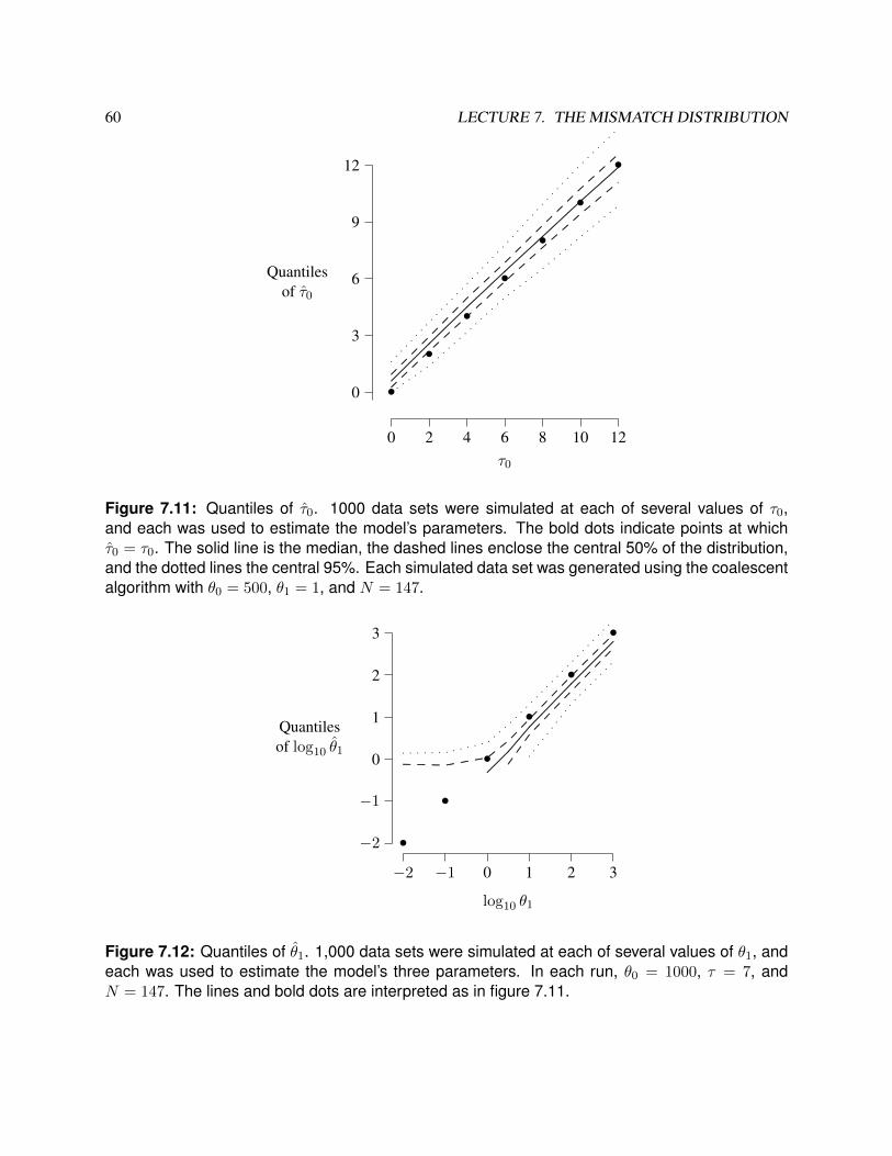
60 LECTURE 7. THE MISMATCH DISTRIBUTION
0
3
6
9
12
Quantilesof τ0
0 2 4 6 8 10 12τ0
•
•
•
•
•
•
•
. .. .
. ....................................
..................................................................................................................................................................................................................................................................................
...........................................................................................................................................................................................................................................................................................................................................................................................................................................................................................................................................................
..............................................................................................................................................................................................................................................................................................
.............................................
Figure 7.11: Quantiles of τ0. 1000 data sets were simulated at each of several values of τ0,and each was used to estimate the model’s parameters. The bold dots indicate points at whichτ0 = τ0. The solid line is the median, the dashed lines enclose the central 50% of the distribution,and the dotted lines the central 95%. Each simulated data set was generated using the coalescentalgorithm with θ0 = 500, θ1 = 1, and N = 147.
−2
−1
0
1
2
3
Quantilesof log10 θ1
−2 −1 0 1 2 3
log10 θ1
•
•
•
•
•
•
..................
...............................................................................................................................................
..........................................................................................................................................................................................................................................................................................................................
............. ............. ............. ............. ............. ............. ..........................
..................................................................................................................................
. . . . . . . . . . . . ........................
Figure 7.12: Quantiles of θ1. 1,000 data sets were simulated at each of several values of θ1, andeach was used to estimate the model’s three parameters. In each run, θ0 = 1000, τ = 7, andN = 147. The lines and bold dots are interpreted as in figure 7.11.

7.B. STATISTICAL PROPERTIES OF POINT ESTIMATES (OPTIONAL) 61
0.0
0.1
Fi
0 5 10 15 20 25
i
↙Africa
............................................
......................................................................................................................................................................
.........................................................................................................................................................................................................................................................................................................................................................................................................................................................................
↙Asia
............................................................................................................................................................................................................................................................................................................................................................................................................................................................................................................................................................................................................................................................................................................................................................................................................................• • •
••• •• •••••• • •
•••••••• • 0.0
0.1
Fi
0 5 10 15 20 25
i
↙Africa
...................................
.............................................................
...............................................................................................................
...................................................................................................................
.........................................................................................................................................................................................................................................................................................................................................................
↙Europe
.......
.......
.......
.......
.......
.......
.......
.......
.......
.......
.......
.......
.......
.......
................................................................................................................................................................................................................................................................................................................................................................................................................................................................................................................................• •••• • •
••••••• •••••••••• •
0.0
0.1
Fi
0 5 10 15 20 25
i
↙Asia
............................................................................................................................................................................................................................................................................................................................................................................................................................................................................................................................................................................................................................................................................................................................................................................................................................
Eur.↘
.......
.......
.......
.......
.......
.......
.......
.......
.......
.......
.......
.......
.......
.......
................................................................................................................................................................................................................................................................................................................................................................................................................................................................................................................................• •
•••••••••••••••••••••••••••• •
Figure 7.13: Mitochondrial Mismatch DistributionsIn each panel, the solid lines show mismatch distributions for within-population comparisons, and the dotted linesshow the analogous between-population comparisons. The data comprise 72 Africans, 77 Asians, and 89 Europeans[13].
62 LECTURE 7. THE MISMATCH DISTRIBUTION
0.11
10θ1
100-fold growth
◦◦◦◦◦◦◦◦
2.5 5 7.5τ0
0.11
10θ1
101-fold growth
◦◦◦◦◦◦◦◦
◦◦◦◦◦◦◦◦
◦◦◦◦◦◦◦
◦◦◦◦◦◦◦◦
◦◦◦◦◦◦◦◦
◦◦◦◦◦◦
◦◦◦◦◦◦◦
◦◦◦◦
◦
◦◦◦◦
◦
2.5 5 7.5τ0
0.11
10θ1
102-fold growth
◦◦◦◦◦◦◦◦
◦◦◦◦◦◦◦◦
◦◦◦◦◦◦◦◦
◦◦◦◦◦◦◦◦
◦◦◦◦◦◦◦◦
◦◦◦◦◦◦◦◦
◦◦◦◦◦◦◦
◦◦◦◦◦◦◦
◦◦◦◦◦◦◦◦
2.5 5 7.5τ0
0.11
10θ1
103-fold growth
◦◦◦◦◦◦◦◦
◦◦◦◦◦◦◦◦
◦◦◦◦◦◦◦◦
◦••••◦◦◦
••••◦◦◦◦
◦◦◦◦◦◦◦
◦◦◦◦◦◦◦◦
◦◦◦◦◦◦◦
◦◦◦◦◦◦◦
2.5 5 7.5τ0
0.11
10θ1
104-fold growth
◦◦◦◦◦◦◦◦
◦◦◦◦◦◦◦◦
◦◦◦◦◦◦◦◦
◦••••◦◦◦
••••◦◦◦◦
◦◦◦◦◦◦◦◦
◦◦◦◦◦◦◦◦
◦◦◦◦◦◦◦
◦◦◦◦◦◦◦◦
2.5 5 7.5τ0
0.11
10θ1
105-fold growth
◦◦◦◦◦◦◦◦
◦◦◦◦◦◦◦◦
◦◦◦◦◦◦◦◦
•••••◦◦◦
••••◦◦◦◦
◦◦◦◦◦◦◦
◦◦◦◦◦◦◦◦
◦◦◦◦◦◦◦◦
◦◦◦◦◦◦◦◦
2.5 5 7.5τ0
0.11
10θ1
106-fold growth
◦◦◦◦◦◦◦◦
◦◦◦◦◦◦◦◦
◦◦◦◦◦◦◦◦
•••••◦◦◦
••••◦◦◦
◦◦◦◦◦◦◦
◦◦◦◦◦◦◦
◦◦◦◦◦◦◦
◦◦◦◦◦◦◦
2.5 5 7.5τ0
0.11
10θ1
107-fold growth
◦◦◦◦◦◦◦◦
◦◦◦◦◦◦◦◦
◦◦◦◦◦◦◦◦
◦••••◦◦◦
••••◦◦◦◦
◦◦◦◦◦◦◦◦
◦◦◦◦◦◦◦◦
◦◦◦◦◦◦◦◦
◦◦◦◦◦◦◦◦
Figure 7.14: An experiment designed to test the method for generating confidence regions.Rather than beginning with a real data set, this experiment began with a simulated data set that was generated underthe assumptions that N = 147, and (τ, θ0, θ1) = (4, 1, 500). A confidence region was then generated as describedin the text. Open circles (◦) represent points outside the 95% confidence region; closed circles (•) represent pointswithin. Note that the correct hypothesis {(τ, θ0, θ1) = (4, 1, 500)} falls inside the confidence region.

7.B. STATISTICAL PROPERTIES OF POINT ESTIMATES (OPTIONAL) 63
0.11
10θ0
100-fold growth
◦◦◦◦◦◦◦◦
5 100.1
110
101-fold growth
◦◦◦◦◦◦
◦◦◦◦◦◦◦◦
◦◦◦◦◦◦◦
◦◦◦◦◦◦◦
◦◦◦◦◦◦◦
◦◦◦◦
◦◦
◦◦◦◦◦◦◦
◦◦◦◦◦◦◦◦
5 100.1
110
θ0
102-fold growth
◦◦◦◦◦◦◦◦
◦◦◦◦◦◦◦◦
◦◦◦◦◦◦◦◦
◦◦◦◦◦◦◦◦
◦◦◦◦◦◦
◦◦◦◦◦◦◦
◦◦◦◦◦◦◦
◦
◦◦◦◦
5 100.1
110
103-fold growth
◦◦◦◦◦◦◦◦
◦◦◦◦◦•◦◦
◦◦◦•••◦◦
◦◦•••◦◦◦
◦◦••◦◦◦◦
◦◦◦◦◦◦
◦◦◦◦◦◦◦◦
◦◦◦◦◦◦◦◦
5 10τ
0.11
10θ0
104-fold growth
◦◦◦◦◦◦◦◦
◦◦◦◦••◦
◦◦◦••◦◦
◦••••◦◦◦
•••◦◦◦◦◦
◦◦◦◦◦◦◦◦
◦◦◦◦◦◦◦
◦◦◦◦◦◦◦◦
5 10τ
0.11
10105-fold growth
◦◦◦◦◦◦◦◦
◦◦◦◦••◦
◦◦◦•••◦◦
◦•••••◦◦
•••◦◦•◦◦
◦◦◦◦◦◦◦◦
◦◦◦◦◦◦◦
◦◦◦◦◦◦◦◦
Figure 7.15: 95% confidence region for the Cann-Stoneking-Wilson dataOpen circles (◦) represent points outside the 95% confidence region; closed circles (•) represent points within. Themarginal confidence regions are τ : [5, 8], θ0 : [0, 4.6], and θ1/θ0 : (100,∞]. If the mutation rate is u = 0.001per sequence per generation, and generations are 25 years, these intervals become t : [62, 100] thousand years, andN0 : [0, 2320] females.

64 LECTURE 7. THE MISMATCH DISTRIBUTION
Lecture 8
Microsatellites
8.1 Repeat polymorphisms: Nomenclature
tandem repeat polymorphisms A particular sequence is repeated again and again. For example, if therepeated sequence is AT, then one chromosome might have a sting of three repeats (ATATAT) andanother might have a string of five (ATATATATAT). They are called “tandem” repeats because therepeated units are stuck together end-to-end. There are several categories of repeat polymorphism:
Minisatellite the repeated unit is fairly large
Microsatellite the repeated unit is small, commonly 2–6 nucleotides.
Short tandem repeat (STR) a synonym for “microsatellite”
dispersed repeat polymorphisms These also consist of a sequence that is repeated again and again, but inthese polymorphisms the repeated units are adjacent to one another. They are not even close together.They are widely dispersed within the genome. The Alu polymorphisms are an example of this class ofpolymorphism.
8.2 Properties relevant to statistical analysis
Rapid evolution Mutation rate in the neighborhood of 1/1000 per generation [38].
Di- and tetra-nucleotide repeats are likely to be neutral A tetranucleotide repeat doesn’t work very wellwithin a reading frame, because each mutation produces a frame-shift mutation, which probably hascatastrophic consequences. Most of the di- and tetra-nucleotide repeats that we find are outside ofreading frames.
Tri-nucleotide repeats are known within reading frames, and some cause genetic disease.
There are lots of microsatellite loci
Mutational process poorly understood Statistical analysis usually assumes that mutations add or subtractone repeat unit with equal probability. The is almost certainly too simple.
65

66 LECTURE 8. MICROSATELLITES
8.3 A sample of 60 STR loci
Figure 8.1 shows the frequency distributions of repeat counts at a sample of 60 tetra-nucleotide repeat locidescribed by Jorde and his colleagues [13, 14]. Each horizontal axis there shows the number of copies ofthe repeat unit, and each vertical axis shows the number of chromosomes in the sample that exhibited thatnumber of copies.

8.3. A SAMPLE OF 60 STR LOCI 67
◦◦◦◦◦
◦
◦
◦
◦◦◦◦◦◦◦◦◦◦◦◦◦◦ ◦◦◦◦◦
◦
◦◦◦◦◦◦◦◦◦◦◦◦◦◦◦◦ ◦◦◦
◦◦◦◦◦
◦
◦◦◦◦◦◦◦◦◦◦◦◦◦ ◦◦◦◦
◦
◦◦
◦
◦◦◦◦◦◦◦◦◦◦◦◦◦◦ ◦
◦◦◦◦
◦
◦
◦
◦◦◦◦◦◦◦◦◦◦◦◦◦◦ ◦◦◦
◦
◦◦◦◦
◦◦◦◦◦◦◦◦◦◦◦◦◦◦
◦◦◦◦◦◦◦
◦◦◦◦
◦
◦◦◦◦◦◦◦◦◦◦ ◦◦
◦
◦◦◦◦◦
◦◦◦◦◦◦◦◦◦◦◦◦◦◦ ◦◦
◦
◦◦◦◦◦◦◦◦◦◦◦◦◦◦◦◦◦◦◦ ◦◦◦
◦
◦
◦
◦◦
◦
◦◦◦◦◦◦◦◦◦◦◦◦◦ ◦◦◦◦
◦
◦◦
◦
◦◦◦◦◦◦◦◦◦◦◦◦◦◦ ◦◦◦◦◦◦
◦◦
◦◦◦◦◦◦◦◦◦◦◦◦◦◦
◦◦
◦
◦
◦◦
◦◦◦◦◦
◦◦◦◦◦◦◦◦◦◦◦ ◦◦◦
◦
◦◦
◦
◦◦◦◦◦◦◦◦◦◦◦◦◦◦◦ ◦◦
◦◦
◦◦◦◦◦◦◦◦◦◦◦◦◦◦◦◦◦◦ ◦◦
◦◦◦
◦
◦◦◦◦◦◦◦◦◦◦◦◦◦◦◦◦ ◦◦
◦
◦
◦
◦
◦
◦
◦◦◦◦◦◦◦◦◦◦◦◦◦◦ ◦◦
◦
◦◦
◦
◦◦◦◦◦◦
◦◦◦◦◦◦◦◦◦◦
◦◦
◦◦
◦
◦◦◦◦◦◦◦◦◦◦◦◦◦◦◦◦◦ ◦◦◦◦◦
◦◦
◦◦
◦◦◦◦◦◦◦◦◦◦◦◦◦ ◦◦
◦
◦◦◦◦◦◦◦◦
◦◦
◦
◦◦◦◦◦◦◦◦ ◦◦◦◦
◦◦
◦
◦
◦
◦
◦
◦◦◦◦◦◦◦◦◦◦◦ ◦◦◦◦
◦
◦
◦
◦
◦◦◦◦◦◦◦◦◦◦◦◦◦◦ ◦◦◦◦◦◦◦
◦◦
◦
◦◦◦◦◦◦◦◦◦◦◦◦
◦◦◦◦◦◦
◦
◦◦◦◦◦◦◦◦◦◦◦◦◦◦◦ ◦◦◦◦
◦
◦
◦◦◦◦◦◦◦◦◦◦◦◦◦◦◦◦ ◦
◦◦
◦◦◦
◦
◦◦
◦
◦
◦◦◦◦◦◦◦◦◦◦◦ ◦◦◦◦
◦
◦
◦◦◦◦◦◦◦◦◦◦◦◦◦◦◦◦ ◦◦◦
◦
◦◦
◦
◦
◦
◦◦◦◦◦◦◦◦◦◦◦◦◦ ◦◦
◦
◦
◦
◦
◦◦◦◦◦◦◦◦◦◦◦◦◦◦◦◦
◦◦
◦◦
◦◦
◦◦◦◦◦◦◦◦◦◦◦◦◦◦◦◦ ◦◦◦◦◦
◦◦◦◦◦◦
◦
◦◦◦◦◦◦◦◦◦◦ ◦◦◦
◦◦◦◦◦◦◦◦◦
◦
◦◦◦◦◦◦◦◦◦ ◦
◦
◦
◦
◦◦◦◦◦◦◦◦◦◦◦◦◦◦◦◦◦◦ ◦◦
◦
◦
◦
◦
◦◦◦◦◦◦◦◦◦◦◦◦◦◦◦◦ ◦◦
◦
◦◦◦◦
◦◦
◦◦◦◦◦◦◦◦◦◦◦◦◦
◦◦◦◦◦◦◦◦◦
◦
◦◦
◦
◦◦◦◦◦◦◦◦◦ ◦◦◦◦
◦
◦
◦
◦◦◦◦◦◦◦◦◦◦◦◦◦◦◦ ◦◦◦◦
◦
◦◦
◦
◦◦◦◦◦◦◦◦◦◦◦◦◦◦ ◦◦◦
◦
◦◦◦◦◦
◦◦
◦
◦◦◦
◦
◦◦◦◦◦◦ ◦◦◦
◦
◦
◦◦
◦
◦◦◦
◦◦◦◦◦◦◦◦◦◦◦ ◦◦◦
◦
◦
◦◦◦◦◦◦◦◦◦◦◦◦◦◦◦◦◦
◦◦◦◦◦◦
◦◦
◦◦◦◦◦◦◦◦◦◦◦◦◦◦ ◦◦◦
◦
◦
◦
◦◦
◦
◦◦◦◦◦◦◦◦◦◦◦◦◦ ◦
◦◦
◦
◦
◦◦◦◦◦◦◦◦◦◦◦◦◦◦◦◦◦ ◦◦◦
◦
◦
◦◦
◦◦◦◦◦◦◦◦◦◦◦◦◦◦◦ ◦◦◦
◦
◦
◦◦◦◦◦◦◦◦◦◦◦◦◦◦◦◦◦ ◦◦
◦
◦◦◦
◦
◦◦
◦◦◦◦◦◦◦◦◦◦◦◦◦
◦◦
◦
◦◦
◦◦
◦
◦◦◦◦◦◦◦◦◦◦◦◦◦◦ ◦◦◦◦
◦
◦◦
◦◦◦◦◦◦◦◦◦◦◦◦◦◦◦ ◦◦◦◦
◦
◦
◦
◦◦◦◦◦◦◦◦◦◦◦◦◦◦◦ ◦◦◦◦
◦◦
◦
◦◦◦◦◦◦◦◦◦◦◦◦◦◦◦ ◦◦◦
◦
◦
◦◦
◦
◦◦◦◦◦◦◦◦◦◦◦◦◦◦ ◦◦
◦
◦◦◦
◦
◦
◦
◦◦◦◦◦◦◦◦◦◦◦◦◦
0 22◦◦◦◦◦
◦
◦
◦◦◦◦◦◦◦◦◦◦◦◦◦◦◦ ◦◦
◦
◦
◦
◦◦
◦◦◦◦◦◦◦◦◦◦◦◦◦◦◦ ◦◦◦◦◦
◦
◦
◦◦◦◦◦◦◦◦◦◦◦◦◦◦◦ ◦
◦◦◦◦
◦◦◦
◦
◦◦◦
◦
◦
◦◦◦◦◦◦◦◦ ◦◦◦◦◦◦◦
◦◦◦◦
◦◦◦◦
◦◦◦◦◦◦◦ ◦◦◦
◦
◦
◦◦◦◦
◦◦◦
◦◦◦◦◦◦◦◦◦◦
Figure 8.1: Frequency distributions of 60 STR loci
68 LECTURE 8. MICROSATELLITES
8.4 Remark about statistical methods
A variety of statistical methods have been introduced for analysis of STRs. Many of these seem useful, butnone of them have yet become widely used. It is not obvious which should be included in an introductoryaccount.
8.5 Descriptive statistics
Several of the statistical methods used with STRs involve the so-called “moments” of the distribution ofrepeat counts.
The mean For any given locus, the mean is the average number of repeat counts in the sample. Forexample, suppose we had data on 4 haploid genomes with repeat counts 4, 4, 5, and 6. The mean would be
m = (4 + 4 + 5 + 6)/4 = 4.75
The mean is also known as the “first moment” of the distribution.
The variance is the mean squared deviation from the mean. With the data above, this is1
V =((4− 4.75)2 + (4− 4.75)2 + (5− 4.75)2 + (6− 4.75)2
)/4 = 0.6875
The variance is also called the “second moment” of the distribution.
The fourth moment is the mean of the fourth powers of deviations from the mean. With the exampledata,
m4 =((4− 4.75)4 + (4− 4.75)4 + (5− 4.75)4 + (6− 4.75)4
)/4 = 0.7695
Gene identity is defined as usual: it is the probability that a random pair of genes is identical. In theexample data there are 4 genes, so there are (4× 3)/2 = 6 pairs. Only one of these pairs is identical, so thegene identity is
J = 1/6;
This is not a moment of the distribution.
8.6 The method of Kimmel et al [16]
Kimmel et al show that, at equilibrium between mutation and drift,
V = θ
J = 1/√
1 + 2θ
1In a statistics course, you would learn to divide by 3 rather than 4 here in order to obtain an unbiased estimate. I am ignoringsuch niceties.
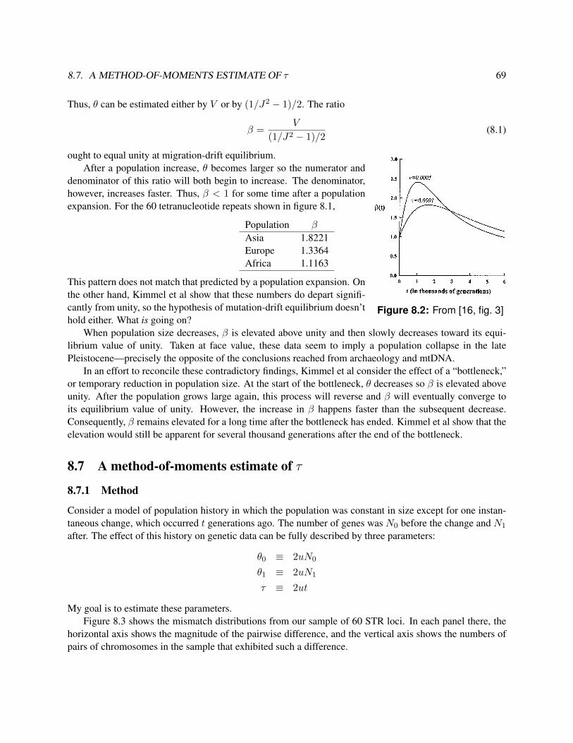
8.7. A METHOD-OF-MOMENTS ESTIMATE OF τ 69
Thus, θ can be estimated either by V or by (1/J2 − 1)/2. The ratio
β =V
(1/J2 − 1)/2(8.1)
ought to equal unity at migration-drift equilibrium.
Figure 8.2: From [16, fig. 3]
After a population increase, θ becomes larger so the numerator anddenominator of this ratio will both begin to increase. The denominator,however, increases faster. Thus, β < 1 for some time after a populationexpansion. For the 60 tetranucleotide repeats shown in figure 8.1,
Population β
Asia 1.8221Europe 1.3364Africa 1.1163
This pattern does not match that predicted by a population expansion. Onthe other hand, Kimmel et al show that these numbers do depart signifi-cantly from unity, so the hypothesis of mutation-drift equilibrium doesn’thold either. What is going on?
When population size decreases, β is elevated above unity and then slowly decreases toward its equi-librium value of unity. Taken at face value, these data seem to imply a population collapse in the latePleistocene—precisely the opposite of the conclusions reached from archaeology and mtDNA.
In an effort to reconcile these contradictory findings, Kimmel et al consider the effect of a “bottleneck,”or temporary reduction in population size. At the start of the bottleneck, θ decreases so β is elevated aboveunity. After the population grows large again, this process will reverse and β will eventually converge toits equilibrium value of unity. However, the increase in β happens faster than the subsequent decrease.Consequently, β remains elevated for a long time after the bottleneck has ended. Kimmel et al show that theelevation would still be apparent for several thousand generations after the end of the bottleneck.
8.7 A method-of-moments estimate of τ
8.7.1 Method
Consider a model of population history in which the population was constant in size except for one instan-taneous change, which occurred t generations ago. The number of genes was N0 before the change and N1
after. The effect of this history on genetic data can be fully described by three parameters:
θ0 ≡ 2uN0
θ1 ≡ 2uN1
τ ≡ 2ut
My goal is to estimate these parameters.Figure 8.3 shows the mismatch distributions from our sample of 60 STR loci. In each panel there, the
horizontal axis shows the magnitude of the pairwise difference, and the vertical axis shows the numbers ofpairs of chromosomes in the sample that exhibited such a difference.

70 LECTURE 8. MICROSATELLITES
◦
◦
◦
◦◦◦◦◦◦◦◦◦◦◦◦◦◦◦◦◦◦◦ ◦
◦
◦◦◦
◦
◦◦◦◦◦◦◦◦◦◦◦◦◦◦◦◦ ◦
◦◦
◦◦◦◦◦◦◦◦◦◦◦◦◦◦◦◦◦◦◦ ◦
◦◦
◦
◦
◦◦◦◦◦◦◦◦◦◦◦◦◦◦◦◦◦ ◦
◦
◦
◦◦◦◦◦◦◦◦◦◦◦◦◦◦◦◦◦◦◦ ◦
◦◦◦◦◦◦◦◦◦◦◦◦◦◦◦◦◦◦◦◦◦
◦
◦◦◦◦◦◦◦◦◦◦◦◦◦◦◦◦◦◦◦◦◦ ◦
◦
◦
◦◦◦
◦◦◦◦◦◦◦◦◦◦◦◦◦◦◦◦ ◦◦
◦
◦
◦
◦◦
◦
◦◦◦◦◦◦◦◦◦◦◦◦◦◦ ◦
◦
◦◦
◦
◦
◦◦◦◦◦◦◦◦◦◦◦◦◦◦◦◦ ◦
◦
◦
◦◦◦◦◦◦◦◦◦◦◦◦◦◦◦◦◦◦◦ ◦
◦
◦
◦◦◦◦◦◦◦◦◦◦◦◦◦◦◦◦◦◦◦
◦
◦
◦◦◦◦◦◦
◦◦◦◦◦◦◦◦◦◦◦◦◦◦ ◦
◦
◦
◦◦◦◦◦◦◦◦◦◦◦◦◦◦◦◦◦◦◦ ◦
◦
◦◦
◦◦◦◦◦◦◦◦◦◦◦◦◦◦◦◦◦◦ ◦
◦
◦
◦◦◦◦◦◦◦◦◦◦◦◦◦◦◦◦◦◦◦ ◦
◦◦
◦◦◦◦◦◦
◦◦◦◦
◦◦◦◦◦◦◦◦◦ ◦
◦
◦◦◦◦◦◦◦◦◦◦
◦◦◦◦◦◦◦◦◦◦
◦
◦
◦
◦
◦
◦◦◦◦◦◦◦◦◦◦◦◦◦◦◦◦◦ ◦
◦
◦◦
◦◦◦◦◦◦◦◦◦◦◦◦◦◦◦◦◦◦ ◦
◦◦◦◦◦◦◦◦◦◦◦◦◦◦◦◦◦◦◦◦◦ ◦
◦
◦
◦
◦
◦◦◦◦◦◦◦◦◦◦◦◦◦◦◦◦◦ ◦
◦
◦
◦◦◦◦◦◦◦◦◦◦◦◦◦◦◦◦◦◦◦ ◦
◦◦
◦◦◦◦◦◦
◦◦◦◦◦◦◦◦◦◦◦◦◦
◦
◦
◦
◦◦◦
◦
◦◦◦◦◦◦◦◦◦◦◦◦◦◦◦ ◦
◦
◦◦◦
◦
◦◦◦◦◦◦◦◦◦◦◦◦◦◦◦◦ ◦
◦◦◦◦◦◦◦◦◦◦◦◦◦◦◦◦◦◦◦◦◦ ◦
◦
◦
◦◦◦◦◦◦◦◦◦◦◦◦◦◦◦◦◦◦◦ ◦
◦
◦◦◦◦◦◦◦◦◦◦◦◦◦◦◦◦◦◦◦◦ ◦
◦
◦
◦◦◦◦◦◦◦◦◦◦◦◦◦◦◦◦◦◦◦
◦
◦
◦
◦◦◦◦◦◦◦◦◦◦◦◦◦◦◦◦◦◦◦ ◦
◦◦◦◦◦◦◦◦◦◦◦◦◦◦◦◦◦◦◦◦◦ ◦
◦◦◦◦◦◦◦◦◦◦◦◦◦◦◦◦◦◦◦◦◦ ◦
◦
◦
◦◦◦◦◦◦◦◦◦◦◦◦◦◦◦◦◦◦◦ ◦
◦◦◦
◦◦
◦◦◦◦◦◦◦◦◦◦◦◦◦◦◦◦ ◦
◦
◦
◦◦
◦◦
◦◦◦◦◦◦◦◦◦◦◦◦◦◦◦
◦
◦
◦◦◦◦◦◦◦◦◦◦◦◦◦◦◦◦◦◦◦◦ ◦
◦
◦◦◦◦
◦◦◦◦◦◦◦◦◦◦◦◦◦◦◦◦ ◦
◦
◦
◦◦◦◦◦◦◦◦◦◦◦◦◦◦◦◦◦◦◦ ◦
◦
◦◦◦◦
◦◦
◦◦◦◦
◦◦◦◦◦◦◦◦◦◦ ◦
◦◦◦◦
◦◦◦◦◦◦◦◦◦◦◦◦◦◦◦◦◦ ◦
◦
◦
◦
◦◦◦◦◦◦◦◦◦◦◦◦◦◦◦◦◦◦
◦
◦
◦◦◦◦
◦◦◦◦◦◦◦◦◦◦◦◦◦◦◦◦ ◦
◦◦◦
◦◦
◦◦◦◦◦◦◦◦◦◦◦◦◦◦◦◦ ◦
◦
◦◦
◦◦◦◦◦◦◦◦◦◦◦◦◦◦◦◦◦◦ ◦
◦
◦
◦◦◦◦◦◦◦◦◦◦◦◦◦◦◦◦◦◦◦ ◦
◦
◦◦
◦
◦◦◦◦◦◦◦◦◦◦◦◦◦◦◦◦◦ ◦
◦◦
◦◦
◦◦◦◦◦◦◦◦◦◦◦◦◦◦◦◦◦
◦
◦
◦◦◦◦◦◦◦◦◦◦◦◦◦◦◦◦◦◦◦◦ ◦
◦◦
◦◦
◦◦◦◦◦◦◦◦◦◦◦◦◦◦◦◦◦ ◦
◦
◦
◦◦◦◦◦◦◦◦◦◦◦◦◦◦◦◦◦◦◦ ◦
◦
◦
◦◦◦◦◦◦◦◦◦◦◦◦◦◦◦◦◦◦◦ ◦
◦
◦
◦◦◦◦◦◦◦◦◦◦◦◦◦◦◦◦◦◦◦ ◦
◦
◦◦◦◦◦◦
◦◦◦◦◦◦◦◦◦◦◦◦◦◦
0 22◦
◦
◦◦◦
◦
◦◦◦◦◦◦◦◦◦◦◦◦◦◦◦◦ ◦
◦
◦
◦◦◦◦◦◦◦◦◦◦◦◦◦◦◦◦◦◦◦ ◦
◦
◦◦◦
◦
◦◦◦◦◦◦◦◦◦◦◦◦◦◦◦◦ ◦
◦◦◦◦◦◦◦◦◦◦◦◦◦◦◦◦◦◦◦◦◦ ◦
◦◦◦◦◦◦◦◦◦◦◦◦◦◦◦◦◦◦◦◦◦ ◦
◦◦◦◦◦◦◦◦◦◦◦◦◦◦◦◦◦◦◦◦◦
Figure 8.3: Mismatch distributions of 60 STR loci

8.7. A METHOD-OF-MOMENTS ESTIMATE OF τ 71
Doing theory with samples of size 2 Rather than attempt a statistical theory for mismatch distributionsfrom samples of size n, I work instead with theory for samples of size 2. This simpler theory should providesome guidance, since the expected values of the components of a mismatch distribution do not depend onsample size [24, footnote 4, p. 61]. Nonetheless, other statistical properties do depend on sample size,so caution is in order. The simple theory of random pairs will provide insight concerning which statisticsare likely to be useful. Before these insights can be trusted, however, they must be tested by computersimulation.
The stepwise mutation model I use a very simple model of mutation, which assumes that each mutationeither adds or subtracts exactly one repeat unit, the two alternatives having equal probability.
We already have a theory describing the effect of population history on mutational differences [19, 25],and the stepwise mutational assumption makes it easy to calculate the probability that two chromosomesdiffer by y repeat units given that they are separated by x mutations.
Figure 8.4 shows the effect of two population histories. The distribution of mutational changes showsa pronounced wave whose position reflects the time of the population expansion. This principle has proveduseful in estimating expansion times from mitochondrial sequence data, where most mutations can be de-tected in comparisons between sequences [23]. But the lower panel shows that the distribution of stepwisedifferences is far less sensitive to differences in population history. Each mutation has an even chanceof erasing the effect of the preceding mutation, and changes in the distribution are subtle. On the otherhand, our sample of 60 STR polymorphisms provides information about 60 essentially independent genegenealogies, whereas the mtDNA provide information about just one. It is not yet clear which will be moreinformative.
The different histories shown in figure 8.4 leave the mode of the stepwise mismatch distribution un-changed but do affect its width. Thus, it seems natural to look for look for effects on the moments of thedistribution (defined above). One can obtain estimators of θ0 and τ by equating the moments of the samplewith theoretical moments in a sample of size 2. This gives
θ0 =√
(m4 − V )/3− V 2 (8.2)
τ = V − θ0 (8.3)
These formulas are analogous to the two-parameter method of moments estimators introduced in lecture 7.There is no estimator for θ1 here because the formulas assume that θ1 is extremely large. They are not likelyto be useful unless the population has in fact expanded.
To verify that these formulas are useful as estimators, I examined their behavior with simulated data. Ateach of a series of values of τ , I generated 1000 10-locus data sets and calculated τ using each data set. Thedistribution of the results, shown in figure 8.5, is gratifying. The sampling distribution of the estimator isrelatively narrow and its central tendency increases in response to increases in τ . There is a modest upwardbias, but since this bias can be measured, it can be corrected. The behavior of θ0, shown in figure 8.6, is lessencouraging. The sampling distribution is wide and its central tendency varies little in response to changesin θ0. Thus, θ0 does not appear to be a useful estimator of θ0.
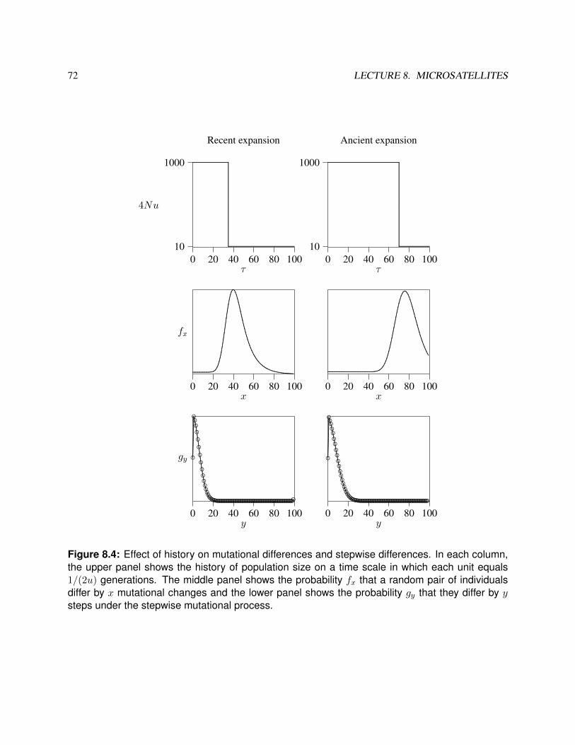
72 LECTURE 8. MICROSATELLITES
Recent expansion
10
1000
4Nu
0 20 40 60 80 100τ
................................................................................................................................................................................................................................................................................................................................................................................................................................................................................................................
0 20 40 60 80 100x
fx
......................................................................................................................................................................................................................................................................................................................................................................................................................................................................................................................................................................................................................................................
0 20 40 60 80 100y
gy ...............................................................................................................................................................................................................................................................................................................................................................................................................................................................................................................................................................................................................
◦
◦◦◦◦◦◦◦◦◦◦◦◦◦◦◦◦◦◦◦◦◦◦◦◦◦◦◦◦◦◦◦◦◦◦◦◦◦◦◦◦◦◦◦◦◦◦◦◦◦◦◦◦◦◦◦◦◦◦◦◦◦◦◦◦◦◦◦◦◦◦◦◦◦◦◦◦◦◦◦◦◦◦◦◦◦◦◦◦◦◦◦◦◦◦◦◦◦◦◦
Ancient expansion
10
1000
0 20 40 60 80 100τ
................................................................................................................................................................................................................................................................................................................................................................................................................................................................................................................
0 20 40 60 80 100x
.........................................................................................................................................................................................................................................................................................................................................................................................................................................................................................................................................................................................................
0 20 40 60 80 100y
........
........
........
........
........
........
........
........
........
........
........
........
........
.....................................................................................................................................................................................................................................................................................................................................................................................................................................................................................
◦
◦◦◦◦◦◦◦◦◦◦◦◦◦◦◦◦◦◦◦◦◦◦◦◦◦◦◦◦◦◦◦◦◦◦◦◦◦◦◦◦◦◦◦◦◦◦◦◦◦◦◦◦◦◦◦◦◦◦◦◦◦◦◦◦◦◦◦◦◦◦◦◦◦◦◦◦◦◦◦◦◦◦◦◦◦◦◦◦◦◦◦◦◦◦◦◦◦◦
Figure 8.4: Effect of history on mutational differences and stepwise differences. In each column,the upper panel shows the history of population size on a time scale in which each unit equals1/(2u) generations. The middle panel shows the probability fx that a random pair of individualsdiffer by x mutational changes and the lower panel shows the probability gy that they differ by ysteps under the stepwise mutational process.
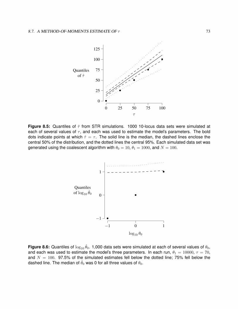
8.7. A METHOD-OF-MOMENTS ESTIMATE OF τ 73
0
25
50
75
100
125
Quantilesof τ
0 25 50 75 100τ
•
•
•
•
•
. .. .
. .. .
. .. .
. .. .
. .. . . . . . . . .
. .. .
. .
..........................
..........................
..........................
..........................
..........................
..........................
..........................
..........................
.................
...........................................................................................................................................................................................................................................................................................................................................................................................................................................................
..........................
..........................
..........................
..........................
..........................
..........................
..........................
......................................................
. .. .
. .. .
. .............................
Figure 8.5: Quantiles of τ from STR simulations. 1000 10-locus data sets were simulated ateach of several values of τ , and each was used to estimate the model’s parameters. The bolddots indicate points at which τ = τ . The solid line is the median, the dashed lines enclose thecentral 50% of the distribution, and the dotted lines the central 95%. Each simulated data set wasgenerated using the coalescent algorithm with θ0 = 10, θ1 = 1000, and N = 100.
−1
0
1
Quantilesof log10 θ0
−1 0 1
log10 θ0
•
•
•............. ............. ............. ............. ............. ............. ............. ............. ............. ............. ............. ............. ............. ............. ............
. . . . . . . . . . . . . . . . . . . . . . . . . . . . . .
Figure 8.6: Quantiles of log10 θ0. 1,000 data sets were simulated at each of several values of θ0,and each was used to estimate the model’s three parameters. In each run, θ1 = 10000, τ = 70,and N = 100. 97.5% of the simulated estimates fell below the dotted line; 75% fell below thedashed line. The median of θ0 was 0 for all three values of θ0.
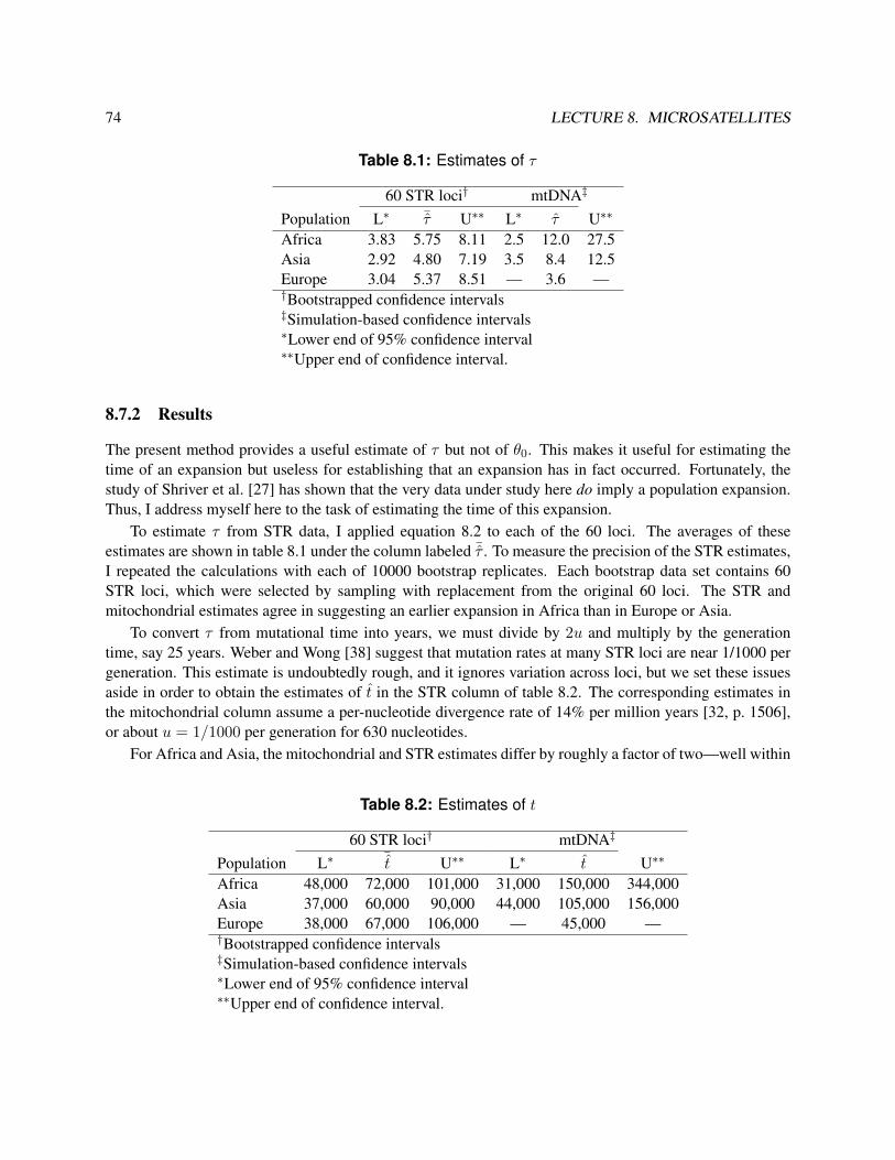
74 LECTURE 8. MICROSATELLITES
Table 8.1: Estimates of τ
60 STR loci† mtDNA‡
Population L∗ ¯τ U∗∗ L∗ τ U∗∗
Africa 3.83 5.75 8.11 2.5 12.0 27.5Asia 2.92 4.80 7.19 3.5 8.4 12.5Europe 3.04 5.37 8.51 — 3.6 —†Bootstrapped confidence intervals‡Simulation-based confidence intervals∗Lower end of 95% confidence interval∗∗Upper end of confidence interval.
8.7.2 Results
The present method provides a useful estimate of τ but not of θ0. This makes it useful for estimating thetime of an expansion but useless for establishing that an expansion has in fact occurred. Fortunately, thestudy of Shriver et al. [27] has shown that the very data under study here do imply a population expansion.Thus, I address myself here to the task of estimating the time of this expansion.
To estimate τ from STR data, I applied equation 8.2 to each of the 60 loci. The averages of theseestimates are shown in table 8.1 under the column labeled ¯τ . To measure the precision of the STR estimates,I repeated the calculations with each of 10000 bootstrap replicates. Each bootstrap data set contains 60STR loci, which were selected by sampling with replacement from the original 60 loci. The STR andmitochondrial estimates agree in suggesting an earlier expansion in Africa than in Europe or Asia.
To convert τ from mutational time into years, we must divide by 2u and multiply by the generationtime, say 25 years. Weber and Wong [38] suggest that mutation rates at many STR loci are near 1/1000 pergeneration. This estimate is undoubtedly rough, and it ignores variation across loci, but we set these issuesaside in order to obtain the estimates of t in the STR column of table 8.2. The corresponding estimates inthe mitochondrial column assume a per-nucleotide divergence rate of 14% per million years [32, p. 1506],or about u = 1/1000 per generation for 630 nucleotides.
For Africa and Asia, the mitochondrial and STR estimates differ by roughly a factor of two—well within
Table 8.2: Estimates of t
60 STR loci† mtDNA‡
Population L∗ ¯t U∗∗ L∗ t U∗∗
Africa 48,000 72,000 101,000 31,000 150,000 344,000Asia 37,000 60,000 90,000 44,000 105,000 156,000Europe 38,000 67,000 106,000 — 45,000 —†Bootstrapped confidence intervals‡Simulation-based confidence intervals∗Lower end of 95% confidence interval∗∗Upper end of confidence interval.

8.7. A METHOD-OF-MOMENTS ESTIMATE OF τ 75
the range of statistical error. For Europe, the two estimates are even closer. Thus, the STR estimates are inbroad agreement with the mitochondrial estimates.
The confidence intervals are narrower with STR data than with mitochondrial data. The mitochondrialinterval is six times as long as the STR interval for Africa and twice as long for Asia. For Europe, themtDNA interval is infinite, but the STR interval is 68,000 years. Thus, STR estimates are appreciably moreprecise. This difference may reflect either the increased information available when one studies 60 locirather than one, or possibly a lack of efficiency in the statistical method used for mtDNA.

76 LECTURE 8. MICROSATELLITES

Lecture 9
Alu Insertions
9.1 What is an Alu insertion?
Transposable elements are DNA sequences that can copy themselves and insert the copies into differentparts of the genome.
• constitute large fractions of eukaryotic genomes
• “selfish DNA”: they don’t have any function that we know of
Short Interspersed Elements (SINEs) are short retroposons (typically 75–500bp) that lack the machineryneeded to transpose themselves. They must be produced by active sites somewhere in the genome, butthe details of this process are mysterious. They are present in huge numbers in eukaryotic genomes.
Alu insertions are SINEs that contain roughly 300bp and are present in huge numbers within the humangenome.
How many? Alus constitute 10.6% of the genome, or just over 290 Mb [18].
Probably neutral (Substitution rate is comparable to that of other non-coding genomic regions.)
9.2 The “master gene” model
It is thought that only a few Alus are capable of transposing. These give rise to all the others. Most of theAlu elements in our genomes are inert.
Families of Alus are defined on the basis of mutations that (presumably) accumulated in the master copies.Many members of younger families are polymorphic in the human gene pool. This makes them especiallyinteresting in intra-specific population genetics.
9.3 Properties that make Alus interesting
1. Insertions are seldom if ever lost cleanly
77
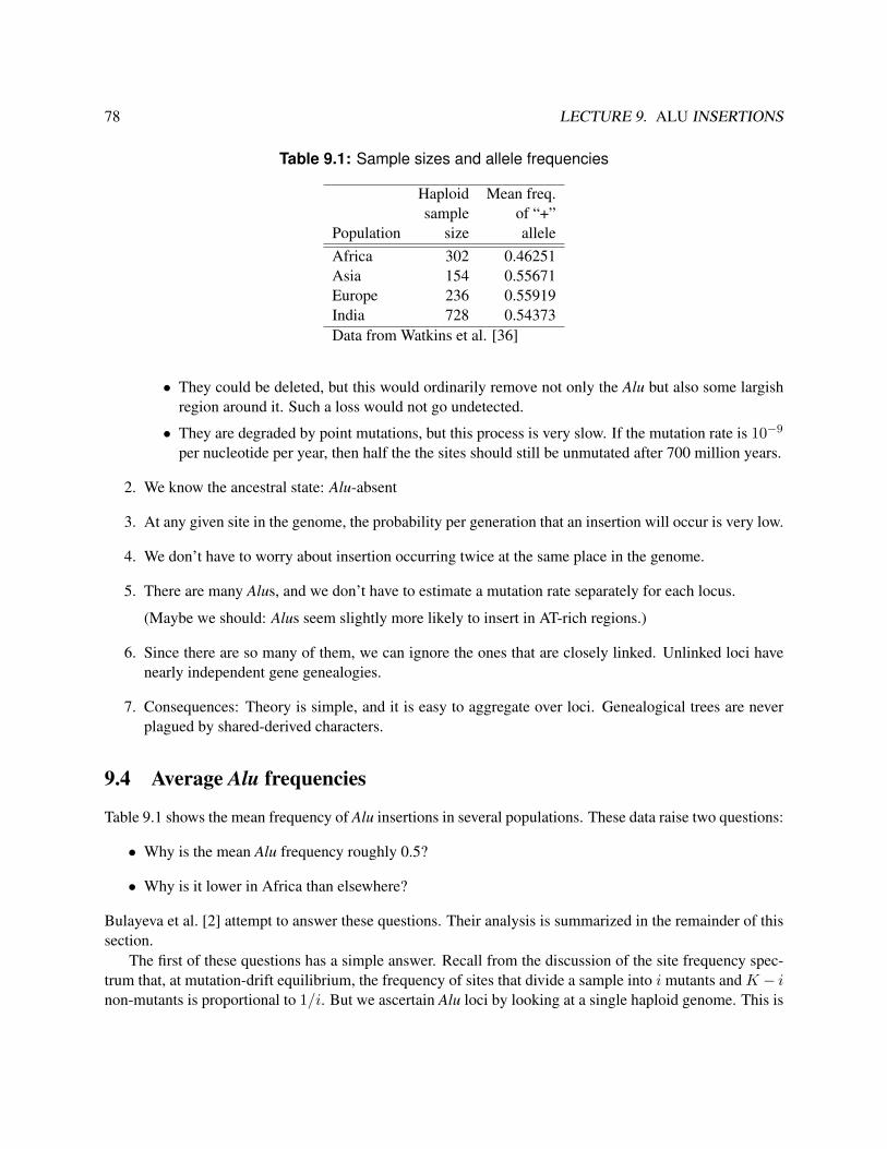
78 LECTURE 9. ALU INSERTIONS
Table 9.1: Sample sizes and allele frequencies
Haploid Mean freq.sample of “+”
Population size alleleAfrica 302 0.46251Asia 154 0.55671Europe 236 0.55919India 728 0.54373Data from Watkins et al. [36]
• They could be deleted, but this would ordinarily remove not only the Alu but also some largishregion around it. Such a loss would not go undetected.
• They are degraded by point mutations, but this process is very slow. If the mutation rate is 10−9
per nucleotide per year, then half the the sites should still be unmutated after 700 million years.
2. We know the ancestral state: Alu-absent
3. At any given site in the genome, the probability per generation that an insertion will occur is very low.
4. We don’t have to worry about insertion occurring twice at the same place in the genome.
5. There are many Alus, and we don’t have to estimate a mutation rate separately for each locus.
(Maybe we should: Alus seem slightly more likely to insert in AT-rich regions.)
6. Since there are so many of them, we can ignore the ones that are closely linked. Unlinked loci havenearly independent gene genealogies.
7. Consequences: Theory is simple, and it is easy to aggregate over loci. Genealogical trees are neverplagued by shared-derived characters.
9.4 Average Alu frequencies
Table 9.1 shows the mean frequency of Alu insertions in several populations. These data raise two questions:
• Why is the mean Alu frequency roughly 0.5?
• Why is it lower in Africa than elsewhere?
Bulayeva et al. [2] attempt to answer these questions. Their analysis is summarized in the remainder of thissection.
The first of these questions has a simple answer. Recall from the discussion of the site frequency spec-trum that, at mutation-drift equilibrium, the frequency of sites that divide a sample into i mutants and K − inon-mutants is proportional to 1/i. But we ascertain Alu loci by looking at a single haploid genome. This is

9.4. AVERAGE ALU FREQUENCIES 79
equivalent to saying that alleles with frequency p should occur with probability proportional to 1/p. Mean-while, we ascertain Alu loci by looking at a single haploid genome. If a locus has allele frequency p, weascertain it with probability p. Thus, the probability that a locus in our sample will have allele frequency pis proportional to 1/p × p = 1. In other words, our sample should contain equal numbers of loci in everyfrequency category. The average of this uniform distribution is 1/2, in good agreement with the data.
9.4.1 Tests of two hypotheses
We are already in a position to test two hypotheses from the literature.
Homo erectus diaspora (HED) hypothesis is an otherwise-plausible hypothesis [11] that is falsified bythese data:
• Homo erectus dispersed out of Africa 1.8 mya, or 72,000 generations ago.
• Consequently, many nuclear gene trees are roughly this deep.
• Neutral theory says that expected time to LCA is 4Ne generations.
• Setting 4Ne = 72, 000 gives Ne = 18, 000.
• This is in fair agreement with Ne as estimated from a variety of nuclear loci.
• Simulations show that, under this hypothesis, the world mean Alu frequency would be smaller than0.19. This did not happen.
Pleistocene population explosion
• Human mitochondrial mismatch distributions suggest that population expanded by several-hundred-fold between 30 kya and 130 kya.
• This would lead to an excess of low-frequency Alus.
• Simulation shows that a history in which human numbers expanded from 3,000 to 300,000 at 5,000generations ago would lead to a world mean Alu frequency between 0.30 and 0.40 in samples of 100Alus.
• This is also excluded by the data.
9.4.2 Why are Alu frequencies higher outside Africa?
To answer this question, we need a model.
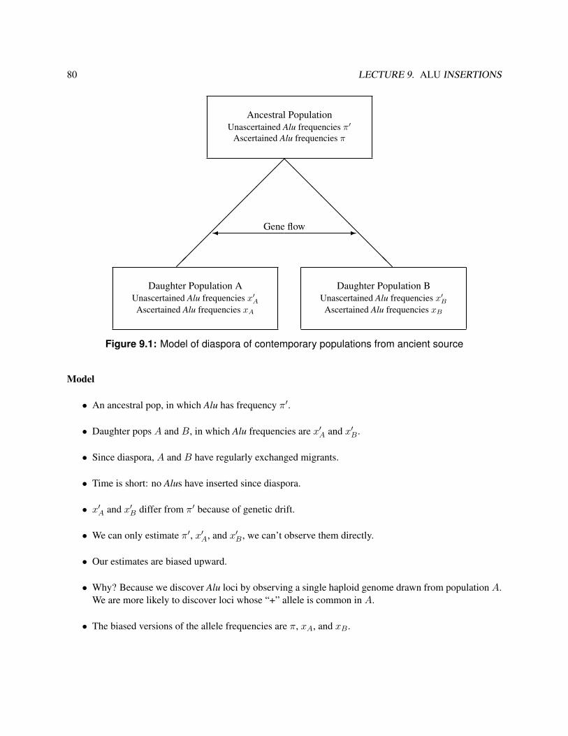
80 LECTURE 9. ALU INSERTIONS
Ancestral PopulationUnascertained Alu frequencies π′
Ascertained Alu frequencies π
Daughter Population AUnascertained Alu frequencies x′AAscertained Alu frequencies xA
Daughter Population BUnascertained Alu frequencies x′BAscertained Alu frequencies xB
��
���
���
��
��
@@@@@@@@@@@@
Gene flow� -
Figure 9.1: Model of diaspora of contemporary populations from ancient source
Model
• An ancestral pop, in which Alu has frequency π′.
• Daughter pops A and B, in which Alu frequencies are x′A and x′B .
• Since diaspora, A and B have regularly exchanged migrants.
• Time is short: no Alus have inserted since diaspora.
• x′A and x′B differ from π′ because of genetic drift.
• We can only estimate π′, x′A, and x′B , we can’t observe them directly.
• Our estimates are biased upward.
• Why? Because we discover Alu loci by observing a single haploid genome drawn from population A.We are more likely to discover loci whose “+” allele is common in A.
• The biased versions of the allele frequencies are π, xA, and xB .
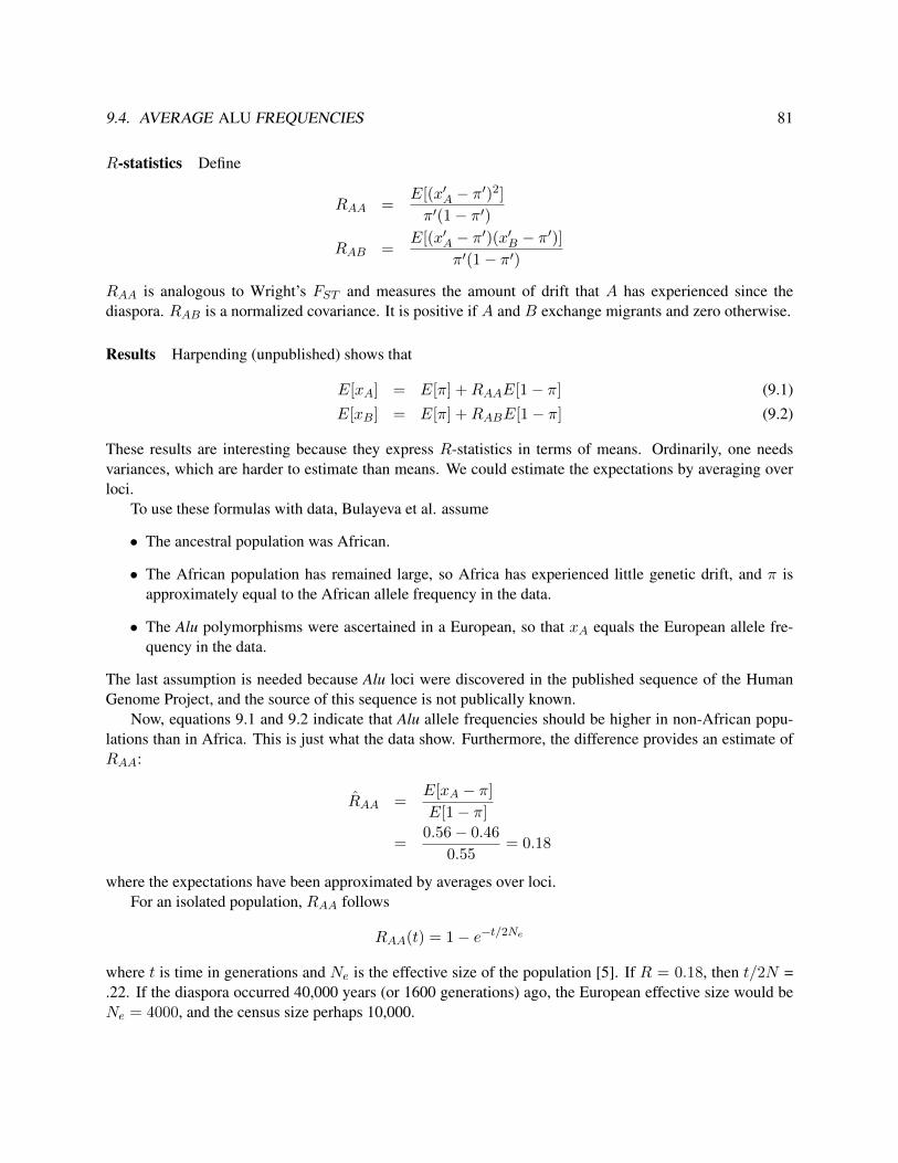
9.4. AVERAGE ALU FREQUENCIES 81
R-statistics Define
RAA =E[(x′A − π′)2]π′(1− π′)
RAB =E[(x′A − π′)(x′B − π′)]
π′(1− π′)
RAA is analogous to Wright’s FST and measures the amount of drift that A has experienced since thediaspora. RAB is a normalized covariance. It is positive if A and B exchange migrants and zero otherwise.
Results Harpending (unpublished) shows that
E[xA] = E[π] +RAAE[1− π] (9.1)
E[xB] = E[π] +RABE[1− π] (9.2)
These results are interesting because they express R-statistics in terms of means. Ordinarily, one needsvariances, which are harder to estimate than means. We could estimate the expectations by averaging overloci.
To use these formulas with data, Bulayeva et al. assume
• The ancestral population was African.
• The African population has remained large, so Africa has experienced little genetic drift, and π isapproximately equal to the African allele frequency in the data.
• The Alu polymorphisms were ascertained in a European, so that xA equals the European allele fre-quency in the data.
The last assumption is needed because Alu loci were discovered in the published sequence of the HumanGenome Project, and the source of this sequence is not publically known.
Now, equations 9.1 and 9.2 indicate that Alu allele frequencies should be higher in non-African popu-lations than in Africa. This is just what the data show. Furthermore, the difference provides an estimate ofRAA:
RAA =E[xA − π]
E[1− π]
=0.56− 0.46
0.55= 0.18
where the expectations have been approximated by averages over loci.For an isolated population, RAA follows
RAA(t) = 1− e−t/2Ne
where t is time in generations and Ne is the effective size of the population [5]. If R = 0.18, then t/2N =.22. If the diaspora occurred 40,000 years (or 1600 generations) ago, the European effective size would beNe = 4000, and the census size perhaps 10,000.
82 LECTURE 9. ALU INSERTIONS
Comments
• The estimate of Ne is in fair agreement with others, even though the method of analysis is verydifferent.
• The method requires knowledge of ancestral state.
• Bias is ordinarily bad, but here it is crucial to the analysis.
• Thus, this analysis makes use of the unusual features of Alu elements.
9.5 The study of Sherry et al
This section will not be used in the 2004 version of the course.Sherry et al. [26] report a series of Alu polymorphisms that were ascertained in HeLa cells. (This means
that an element did not appear in the study unless it was present in HeLa.) They also ignored all elements thatwere present in chimpanzees. (I don’t know how many chimpanzees they looked at.) They then screened apanel of 122 humans for each of the 57 elements that they had identified. Of the 57 elements identified, 13turned out to be polymorphic in humans. The remaining 44 were fixed in humans and absent in chimps.
9.5.1 Consequences of insertions in different parts of the gene tree
1. A locus that is polymorphic in humans inserted inside the human gene tree. This is the portion labeled“a” in figure 9.2.
2. A locus that is fixed in humans and absent in chimps inserted along the branch leading from thechimp/human MRCA to the human MRCA. In the figure, this is the sum of parts b and c.
Part a of the tree
The expected length of part a of the tree (including all branches) is
La = 4NK−1∑i=1
1
i
as shown in section 5.1 and it’s depth is
Ta = 4N(1− 1/K)
as shown in section 4.4. Here, K is the number of haploid genomes in the sample and equals 246. Further-more, these DNA polymorphisms are diploid, so N can be interpreted as the population size. Thus,
La = 4N × 6.08 ≈ 24N generations
Ta = 4N(1− 1/246) ≈ 4N generations

9.5. THE STUDY OF SHERRY ET AL 83
Figure 9.2: Figure 1 from Sherry et al
Part b of the tree
If the human/chimp speciation event occurred 4.5 myr (perhaps 225,000 generations) ago, then the lengthof part b is
Tb = 225, 000− 4N generations
Part c of the tree
This part of the tree represents the coalescence time of a pair of genes within the species ancestral to humansand chimps. On average, it should equal
Tc = 2Nc generations
84 LECTURE 9. ALU INSERTIONS
where Nc is the size of the ancestral species. Takahata et al. [29] estimate that Nc ≈ 100, 000. If this isright, then
Tc = 200, 000 generations
9.5.2 Data analysis
The total branch length isLa + Tb + Tc = 20N + 425000
The sample includes insertions that occur anywhere within these branches. Only a fraction of these muta-tions are polymorphic, however: those occuring in region a, which has length 24N . The fraction of poly-morphic insertions ought to equal (on average) the fraction of the total branch length that holds polymorphicinsertions. In other words,
13
57=
LaLa + Tb + Tc
=24N
20N + 425000
This givesN = 4986
as an estimate of the effective human population size. This is very close to the estimate obtained frommtDNA.
9.6 Ascertainment bias
Unfortunately, the estimate just obtained is biased. The problem is that we only included Alus that werepresent in HeLa cells.
9.7 Exercises
? EXERCISE 9–1 How would the estimate of N have changed if 26 of the 57 Alus has been polymorphic?

9.7. EXERCISES 85
Locus A
A4••A3
A1
A2
B4•
Locus B
B3 •
B1 •
B2 •
Figure 9.3: Haploid (and diploid) ascertainment on a large and a small genealogy

86 LECTURE 9. ALU INSERTIONS
Appendix A
Mean, Variance and Covariance
This is not really a lab exercise. It is a summary and description of concepts of mean, variance, and covari-ance. It is meant to familiarize you with notation and concepts that are used elsewhere.
A.1 The mean
Given a set of numbers such as
x1 = 10, x2 = 12, x3 = 10, x4 = 8
the mean isx = (10 + 12 + 10 + 8)/4 = 10
which can also be written in several other ways, including
x = (x1 + x2 + x3 + x4)/4 =
( 4∑i=1
xi
)/4
In this example there are four elements in the sum. Often the number of elements is represented by a symbolsuch as N . Then
x = N−1N∑i=1
xi
The limits of summation are sometimes omitted, as in
x = N−1∑i
xi
which means that the sum is over all values of i, which here runs from 1 through 4.It is often more convenient to express the mean in terms of the frequencies of elements with particular
values. For example, let nx denote the number of elements with value x. In our example, n1 = n2 = · · · =n7 = 0, n8 = 1, n9 = 0, n10 = 2, n11 = 0, and n12 = 1. With this notation,
x = N−1∑x
xnx
87

88 APPENDIX A. MEAN, VARIANCE AND COVARIANCE
andN =
∑x
nx
Yet another formulation defines the relative frequency of elements with value x by px = nx/N . Then
p8 = p12 = 1/4, and p10 = 1/2
and the mean can be written asx =
∑x
xpx
In this formulation, px is the relative frequency of value x in the data.The same formula also turns up in probability theory. Suppose that some variable, X , takes values that
cannot be predicted exactly, but which occur with specified probabilities, p1, p2, . . . . Then X is called a“random variable” and its expectation, E[x], is defined as
E[X] =∑x
xpx
Note that this is the same as the preceding formulation of the mean.Finally, suppose that X is a continuous variable, such as stature, that takes values over the range from a
to b. Then you cannot enumerate the possible values that it may take. Its expectation, or average value, iswritten as
E[X] =
∫ b
axf(x)dx
where f(x)dx can be thought of as the probability that X takes a value within the (very small) interval fromx to x+ dx, and is thus analagous to px in the discrete formulation.
A.2 Variance
The variance of a series of numbers is the average squared difference from the mean. For example, the meanof the numbers listed above is 10, so the variance is
V = ((10− 10)2 + (12− 10)2 + (10− 10)2 + (8− 10)2)/4 = 2
As with the mean, there is a variety of ways to represent the variance, including
V = N−1∑i
(xi − x)2 (A.1)
=∑x
(x− x2)px
=∑x
x2px − x2 (A.2)
= x2 − x2 (A.3)
The last line says that the variance is the mean square of x minus the squared mean.Equation A.1 provides the most straightforward method of calculating the variance, but it requires two
passes through the data. The first pass calculates the mean, and the second sums the squared deviations fromthe mean. Equation A.3 is often more convenient because it requires only one pass through the data.
A.3. COVARIANCES 89
? EXERCISE A–1 Verify that these formulas are equivalent.
In probability theory, the (theoretical) variance is defined as
V [X] = E[(X − E[X])2
]= E[X2]− (E[X])2
These expressions hold irrespective of whether the random variable is continuous or discrete, but they haveslightly different interpretations in the two cases. For discrete random variables,
E[X2] =∑x
x2px
but for continuous random variablesE[X2] =
∫x2f(x)dx
A.3 Covariances
The covariance of two sets of numbers, x1, . . . , xN , and y1, . . . , yN , is
Cov(x, y) =N∑i=1
(xi − x)(yi − y)
where x and y are the means of the two sets of numbers. Alternate expressions for the covariance include
Cov(x, y) =∑x
∑y
(x− x)(y − y)px,y
=∑xy
(x− x)(y − y)px,y
=∑xy
xypx,y − xy (A.4)
Here px,y is the relative frequency of pairs of numbers with values (x, y) and the sum is taken over allpossible of pairs of numbers. The notation
∑xy means the same thing as
∑x
∑y.

90 APPENDIX A. MEAN, VARIANCE AND COVARIANCE

Bibliography
[1] A.M. Bowcock, A. Ruiz-Linares, J. Tomfohrde, E. Minch, J.R. Kidd, and L. Luca Cavalli-Sforza. Highresolution of human evolutionary trees with polymorphic microsatellites. Nature, 368:455–457, March1994.
[2] Kazima Bulayeva, Lynn B. Jorde, Christopher Ostler, Scott Watkins, Oleg Bulayev, and Henry Harp-ending. Genetics and population history of Caucasus populations. Human Biology, 75(6):837–853,2003.
[3] Rebecca L. Cann, Mark Stoneking, and Allan C. Wilson. Mitochondrial DNA and human evolution.Nature, 325(1):31–36, January 1987.
[4] Andrew G. Clark, Kennety M. Weiss, Deborah A. Nickerson, Scott L. Taylor, Anne Buchanan, JariStengard, Veikko Salomaa, Erkki Vartiainen, Markus Perola, Eric Boerwinkle, and Charles F. Sing.Haplotype structure and population genetic inferences from nucleotide-sequence variation in humanLipoprotein Lipase. American Journal of Human Genetics, 63:595–612, 1998.
[5] James F. Crow and Motoo Kimura. An Introduction to Population Genetics Theory. Harper and Row,New York, 1970.
[6] Yunxin Fu. Statistical properties of segregating sites. Theoretical Population Biology, 48(2):172–197,October 1995.
[7] Marc K. Halushka, Jian-Bing Fan, Kimberly Bently, Linda Hsie, Naiing Shen, Alan Weder, RichardCooper, Robert Lipshutz, and Aravinda Chakravarti. Patterns of single-nucleotide polymorphisms incandidate genes for blood-pressure homeostasis. Nature Genetics, 22:239–247, 1999.
[8] Rosalind M. Harding, S. M. Fullerton, R. C. Griffiths, Jacquelyn Bond, Martin J. Cox, Julie A. Schnei-der, Danielle S. Moulin, and J. B. Clegg. Archaic African and Asian lineages in the genetic ancestryof modern humans. American Journal of Human Genetics, 60:722–789, 1997.
[9] Henry C. Harpending, Mark A. Batzer, Michael Gurven, Lynn B. Jorde, Alan R. Rogers, andStephen T. Sherry. Genetic traces of ancient demography. Proceedings of the National Academyof Sciences, USA, 95:1961–1967, 1998.
[10] Eugene E. Harris and Jody Hey. X chromosome evidence for ancient human histories. Proceedingsof the National Academy of Sciences, USA, 96:3320–3324, 1999. URL http://www.pnas.org/cgi/content/full/96/6/3320.
91

92 BIBLIOGRAPHY
[11] John K. Hawks, K. Hunley, S. H. Lee, et al. Population bottlenecks and Pleistocene human evolution.Molecular Biology and Evolution, 17(1):2–22, 2000.
[12] Richard R. Hudson. Gene genealogies and the coalescent process. In Douglas Futuyma and JanisAntonovics, editors, Oxford Surveys in Evolutionary Biology, volume 7, pages 1–44. Oxford UniversityPress, Oxford, 1990.
[13] Lynn B. Jorde, M. J. Bamshad, W. S. Watkins, R. Zenger, A. E. Fraley, P. A. Krakowiak, K. D.Carpenter, H. Soodyall, T. Jenkins, and Alan R. Rogers. Origins and affinities of modern humans:A comparison of mitochondrial and nuclear genetic data. American Journal of Human Genetics, 57:523–538, Sept 1995.
[14] Lynn B. Jorde, Alan R. Rogers, Michael Bamshad, W. Scott Watkins, Patrycia Krakowiak, SandySung, Juha Kere, and Henry C. Harpending. Microsatellite diversity and the demographic history ofmodern humans. Proceedings of the National Academy of Sciences, USA, 94:3100–3103, April 1997.
[15] Henrik Kaessmann, Florian Heißig, Arndt von Haeseler, and Svante Paabo. DNA sequence variation ina non-coding region of low recombination on the human X chromosome. Nature Genetics, 22:78–81,1999.
[16] Marek Kimmel, Ranajit Chakraborty, J. Patrick King, Michael Bamshad, W. Scott Watkins, andLynn B. Jorde. Signatures of population expansion in microsatellite repeat data. Genetics, 148:1921–1930, 1998. http://www.genetics.org/cgi/content/full/148/4/1921.
[17] J. F. C. Kingman. The coalescent. Stochastic Processes and Their Applications, 13:235–248, 1982.
[18] Eric S. Lander et al. Initial sequencing and analysis of the human genome. Nature, 409:860–921,2001.
[19] Wen-Hsiung Li. Distribution of nucleotide differences between two randomly chosen cistrons in afinite population. Genetics, 85:331–337, 1977.
[20] Wen-Hsiung Li. Molecular Evolution. Sinauer, Sunderland, Mass., 1997.
[21] Michael W. Nachman, Vanessa L. Bauer, Susan L. Crowell, and Charles F. Aquadro. DNA variabilityand recombination rates at x-linked loci in humans. Genetics, 150:1133–1141, 1998.
[22] Masatoshi Nei, Gregory Livshits, and Tatsuya Ota. Genetic variation and evolution of human popula-tions. In C. F. Sing and C. L. Hanis, editors, Genetics of Cellular, Individual, Family, and PopulationVariability, pages 239–252. Oxford University Press, Oxford, 1993.
[23] Alan R. Rogers. Genetic evidence for a Pleistocene population explosion. Evolution, 49(4):608–615,August 1995.
[24] Alan R. Rogers. Population structure and modern human origins. In Peter J. Donnelly and SimonTavare, editors, Progress in Population Genetics and Human Evolution, pages 55–79. Springer-Verlag,New York, 1997.
BIBLIOGRAPHY 93
[25] Alan R. Rogers and Henry C. Harpending. Population growth makes waves in the distribution ofpairwise genetic differences. Molecular Biology and Evolution, 9:552–569, 1992.
[26] Stephen T. Sherry, Henry C. Harpending, Mark A. Batzer, and Mark Stoneking. Alu evolution inhuman populations: Using the coalescent to estimate effective population size. Genetics, 147:1977–1982, 1997.
[27] Mark D. Shriver, Li Jin, Robert E. Ferrell, and Ranjan Deka. Microsatellite data support an earlypopulation expansion in Africa. Genome Research, 7:586–591, 1997.
[28] Fumio Tajima. Evolutionary relationship of DNA sequences in finite populations. Genetics, 105:437–460, October 1983.
[29] N. Takahata, Y. Satta, and J. Klein. Divergence time and population size in the lineage leading tomodern humans. Theoretical Population Biology, 48:198–221, 1995.
[30] Simon Tavare. Line-of-descent and genealogical processes, and their applications in population genet-ics models. Theoretical Population Biology, 26:119–164, 1984.
[31] Peter A. Underhill, Li Jin, Alice A. Lin, S. Quasim Mehdi, Trevor Jenkins, Douglas Vollrath,Ronald W. Davis, L. Luca Cavalli-Sforza, and Peter J. Oefner. Detection of numerous Y chromosomebiallelic polymorphisms by denaturing high-performance liquid chromatography. Genome Research,7:996–1005, 1997.
[32] Linda Vigilant, Mark Stoneking, Henry Harpending, Kristen Hawkes, and Allan C. Wilson. Africanpopulations and the evolution of human mitochondrian DNA. Science, 253:1503–1507, 1991.
[33] John Wakeley. Coalescent Theory: An Introduction. Roberts & Company, Greenwood Village, Col-orado, 2009.
[34] R. H. Ward, Barbara L. Frazier, Kerry Dew-Jager, and Svante Paabo. Extensive mitochondrial diversitywithin a single Amerindian tribe. Proceedings of the National Academy of Sciences, USA, 88:8720–8724, 1991.
[35] W. S. Watkins, M. J. Bamshad, A. E. Fraley, and L. B. Jorde. Population genetics of trinucleotiderepeat polymorphisms. Human Molecular Genetics, 4:1485–1491, 1995.
[36] W. S. Watkins, A. R. Rogers, C. T. Ostler, S. Wooding, M. J. Bamshad, A-M. E. Brassington, M. L.Carroll, S. V. Nguyen, J. A. Walker, B. V. Prasad, P. G. Reddy, P. K. Das, M. A. Batzer, and L. B. Jorde.Genetic variation in world populations: Inferences from 100 Alu insertion polymorphisms. GenomeResearch, 13(7):1607–1618, 2003.
[37] G. A. Watterson. On the number of segregating sites in genetical models without recombination.Theoretical Population Biology, 7:256–276, 1975.
[38] J.L. Weber and C. Wong. Mutation of human short tandem repeats. Human Molecular Genetics, 2(8):1123–1128, Aug 1993.

94 BIBLIOGRAPHY
[39] Stephen Wooding and Alan R. Rogers. The matrix coalescent and an application to human SNPs.Genetics, 161:1641–1650, 2002.
[40] Ewa Zietkiewicz, Vania Votova, Michal Jarnik, Maria Koran-Laskowska, Kenneth K. Kidd, DavidModiano, Rosaria Scozzari, Mark Stoneking, Sarah Tishkoff, Mark Batzer, and Damian Labuda. Ge-netic structure of the ancestral population of modern humans. Journal of Molecular Evolution, 47:146–155, 1998.
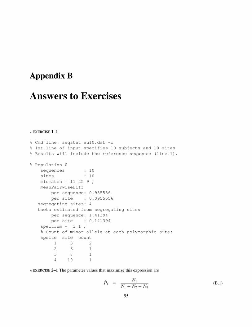
Appendix B
Answers to Exercises
? EXERCISE 1–1
% Cmd line: seqstat eu10.dat -c% 1st line of input specifies 10 subjects and 10 sites% Results will include the reference sequence (line 1).
% Population 0sequences : 10sites : 10mismatch = 11 25 9 ;meanPairwiseDiff
per sequence: 0.955556per site : 0.0955556
segregating sites: 4theta estimated from segregating sites
per sequence: 1.41394per site : 0.141394
spectrum = 3 1 ;% Count of minor allele at each polymorphic site:%psite site count
1 3 22 6 13 7 14 10 1
? EXERCISE 2–1 The parameter values that maximize this expression are
P1 =N1
N1 +N2 +N3(B.1)
95
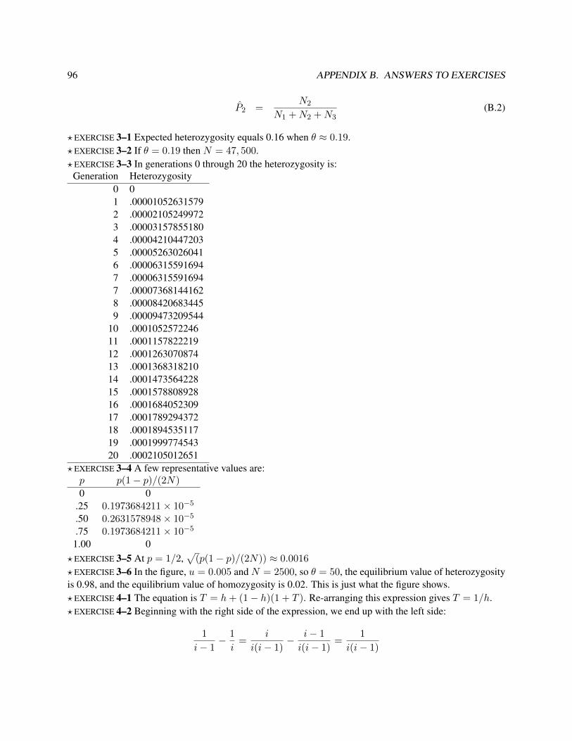
96 APPENDIX B. ANSWERS TO EXERCISES
P2 =N2
N1 +N2 +N3(B.2)
? EXERCISE 3–1 Expected heterozygosity equals 0.16 when θ ≈ 0.19.? EXERCISE 3–2 If θ = 0.19 then N = 47, 500.? EXERCISE 3–3 In generations 0 through 20 the heterozygosity is:
Generation Heterozygosity0 01 .000010526315792 .000021052499723 .000031578551804 .000042104472035 .000052630260416 .000063155916947 .000063155916947 .000073681441628 .000084206834459 .00009473209544
10 .000105257224611 .000115782221912 .000126307087413 .000136831821014 .000147356422815 .000157880892816 .000168405230917 .000178929437218 .000189453511719 .000199977454320 .0002105012651
? EXERCISE 3–4 A few representative values are:p p(1− p)/(2N)
0 0.25 0.1973684211× 10⁻⁵
.50 0.2631578948× 10⁻⁵
.75 0.1973684211× 10⁻⁵
1.00 0? EXERCISE 3–5 At p = 1/2,
√(p(1− p)/(2N)) ≈ 0.0016
? EXERCISE 3–6 In the figure, u = 0.005 and N = 2500, so θ = 50, the equilibrium value of heterozygosityis 0.98, and the equilibrium value of homozygosity is 0.02. This is just what the figure shows.? EXERCISE 4–1 The equation is T = h+ (1− h)(1 + T ). Re-arranging this expression gives T = 1/h.? EXERCISE 4–2 Beginning with the right side of the expression, we end up with the left side:
1
i− 1− 1
i=
i
i(i− 1)− i− 1
i(i− 1)=
1
i(i− 1)

97
? EXERCISE 4–3 The intervals are:i 4N/(i(i− 1))
10 111.11111119 138.88888898 178.57142867 238.09523816 333.33333335 500.00000004 833.33333333 1666.6666672 5000.000000
? EXERCISE 4–4 Since the sample is large, the mean age of the LCA is close to 4N generations. Half of thisperiod is accounted for by the interval during which the tree contained only two lineages.? EXERCISE 5–1 Let xij denote the difference between the ith and jth sequences, and let M denote thenumber of pairs of sequences in the sample. Then π =
∑xij/M , where the sum runs over all i and j such
that i < j. The expected value of π is
E[π] = E[M−1
∑xij]
(definition of π)
= M−1E[∑
xij]
(JEPr eqn. 7)
= M−1∑
[Exij ] (JEPr eqn. 8)
= M−1Mθ (eqn. 5.4 with K = 2)
= θ
Here, JEPr eqn. 7 tells us that E[aX] = aE[X] for constant a and variable X , and JEPr eqn. 8 tells us thatthe expectation of a sum equals the corresponding sum of expectations. Eqn. 5.4 (with K = 2) tells us thatthe expected number of segregating sites in a sample of size 2 is equal to θ. For such samples, the numberof segregating sites is equal to the number of differences between the two sequences.? EXERCISE 6–1 That example was of a sample of K = 10 DNA sequences, which had 15 segregating sites.Thus, we can estimate θ as
θS =15∑9i=1
1i
= 5.3
I’ll use the symbols vu and vf to represent the unfolded and folded spectra respectively. The unfoldedtheoretical spectrum (assuming selective neutrality and constant population size) is
vu = [θ, θ/2, θ/3, . . . , θ/9]
The first entry in this vector is the expected number of singleton sites, the second is the expected number ofdoubleton sites, and so on. Substituting the estimated value of θ turns this into
vu = [5.30, 2.65, 1.77, 1.33, 1.06, 0.88, 0.76, 0.66, 0.59]
The folded spectrum is constructed as follows:
vf = [5.30 + 0.59, 2.65 + 0.66, 1.77 + 0.76, 1.33 + 0.88, 1.06]
= [5.89, 3.31, 2.53, 2.21, 1.06]

98 APPENDIX B. ANSWERS TO EXERCISES
Thus, we expect 5.89 sites at which the minor allele is present in 1 copy, 3.31 sites at which it is present in2 copies, and so on. In the real data (see section 1.3, page 7), we had
vf = [6, 2, 2, 5, 0]
where the “hat” indicates that these values refer to data rather than from theory. The theoretical and observedspectra are similar, but certainly not identical. No inference can be drawn from this difference, because oursample is very small.