lecture notes on static analysis - itu.dk · lecture notes on static analysis michael i....
TRANSCRIPT
Lecture Notes on Static Analysis
Michael I. Schwartzbach
BRICS, Department of Computer Science
University of Aarhus, Denmark
Abstract
These notes present principles and applications of static analysis of
programs. We cover type analysis, lattice theory, control flow graphs,
dataflow analysis, fixed-point algorithms, narrowing and widening, inter-
procedural analysis, control flow analysis, and pointer analysis. A tiny
imperative programming language with heap pointers and function point-
ers is subjected to numerous different static analyses illustrating the tech-
niques that are presented.
The style of presentation is intended to be precise but not overly for-
mal. The readers are assumed to be familiar with advanced programming
language concepts and the basics of compiler construction.
1
Contents
1 Introduction 3
2 A Tiny Example Language 4
Example Programs 6
3 Type Analysis 7
Types 7
Type Constraints 8
Solving Constraints 9
Slack and Limitations 10
4 Lattice Theory 11
Lattices 11
Fixed-Points 12
Closure Properties 13
Equations and Inequations 15
5 Control Flow Graphs 15
Control Flow Graphs for Statements 16
6 Dataflow Analysis 17
Fixed-Point Algorithms 18
Example: Liveness 19
Example: Available Expressions 22
Example: Very Busy Expressions 25
Example: Reaching Definitions 26
Forwards, Backwards, May, and Must 27
Example: Initialized Variables 28
Example: Sign Analysis 28
Example: Constant Propagation 31
7 Widening and Narrowing 32
8 Conditions and Assertions 35
9 Interprocedural Analysis 36
Flow Graphs for Programs 36
Polyvariance 39
Example: Tree Shaking 40
10 Control Flow Analysis 41
Control Flow Analysis for the λ-Calculus 41
The Cubic Algorithm 42
Control Flow Graphs for Function Pointers 44
Class Hierarchy Analysis 46
11 Pointer Analysis 47
Points-To Analysis 47
Andersen’s Algorithm 47
Steensgaard’s Algorithm 49
Interprocedural Points-To Analysis 50
Example: Null Pointer Analysis 51
Example: Shape Analysis 53
Example: Better Shape Analysis 55
Example: Escape Analysis 58
12 Conclusion 58
2
1 Introduction
There are many interesting questions that can be asked about a given program:
• does the program terminate?
• how large can the heap become during execution?
• what is the possible output?
Other questions concern individual program points in the source code:
• does the variable x always have the same value?
• will the value of x be read in the future?
• can the pointer p be null?
• which variables can p point to?
• is the variable x initialized before it is read?
• is the value of the integer variable x always positive?
• what is a lower and upper bound on the value of the integer variable x?
• at which program points could x be assigned its current value?
• do p and q point to disjoint structures in the heap?
Rice’s theorem is a general result from 1953 that informally can be paraphrasedas stating that all interesting questions about the behavior of programs areundecidable. This is easily seen for any special case. Assume for example theexistence of an analyzer that decides if a variable in a program has a constantvalue. We could exploit this analyzer to also decide the halting problem byusing as input the program:
x = 17; if (TM(j)) x = 18;
Here x has a constant value if and only if the j’th Turing machine halts onempty input.
This seems like a discouraging result. However, our real focus is not to decidesuch properties but rather to solve practical problems like making the programrun faster or use less space, or finding bugs in the program. The solution isto settle for approximative answers that are still precise enough to fuel ourapplications.
Most often, such approximations are conservative, meaning that all errorslean to the same side, which is determined by our intended application.
Consider again the problem of determining if a variable has a constant value.If our intended application is to perform constant propagation, then the analysismay only answer yes if the variable really is a constant and must answer no ifthe variable may or may not be a constant. The trivial solution is of course toanswer no all the time, so we are facing the engineering challenge of answeringyes as often as possible while obtaining a reasonable performance.
3
A different example is the question: to which variables may the pointer p
point? If our intended application is to replace *p with x in order to save adereference operation, then the analysis may only answer “&x” if p certainlymust point to x and must answer “?” if this is false or the answer cannot bedetermined. If our intended application is instead to determine the maximal sizeof *p, then the analysis must reply with a possibly too large set {&x,&y,&z,...}that is guaranteed to contain all targets.
In general, all optimization applications need conservative approximations.If we are given false information, then the optimization is unsound and changesthe semantics of the program. Conversely, if we are given trivial information,then the optimization fails to do anything.
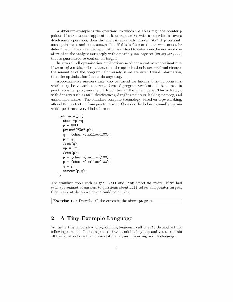
Approximative answers may also be useful for finding bugs in programs,which may be viewed as a weak form of program verification. As a case inpoint, consider programming with pointers in the C language. This is fraughtwith dangers such as null dereferences, dangling pointers, leaking memory, andunintended aliases. The standard compiler technology, based on type checking,offers little protection from pointer errors. Consider the following small programwhich performs every kind of error:
int main() {
char *p,*q;
p = NULL;
printf("%s",p);
q = (char *)malloc(100);
p = q;
free(q);
*p = ’x’;
free(p);
p = (char *)malloc(100);
p = (char *)malloc(100);
q = p;
strcat(p,q);
}
The standard tools such as gcc -Wall and lint detect no errors. If we hadeven approximative answers to questions about null values and pointer targets,then many of the above errors could be caught.
Exercise 1.1: Describe all the errors in the above program.
2 A Tiny Example Language
We use a tiny imperative programming language, called TIP, throughout thefollowing sections. It is designed to have a minimal syntax and yet to containall the constructions that make static analyses interesting and challenging.
4
Expressions
The basic expressions all denote integer values:
E → intconst→ id→ E + E | E - E | E * E | E / E | E > E | E == E→ ( E )
→ input
The input expression reads an integer from the input stream. The comparisonoperators yield 0 for false and 1 for true. Pointer expressions will be added later.
Statements
The simple statements are familiar:
S → id = E;
→ output E;
→ S S→ if (E) { S }→ if (E) { S } else { S }→ while (E) { S }→ var id1,. . . ,,idn;
In the conditions we interpret 0 as false and all other values as true. The outputstatement writes an integer value to the output stream. The var statementdeclares a collection of uninitialized variables.
Functions
Functions take any number of arguments and return a single value:
F → id ( id,. . . ,id ) { var id,. . .,id; S return E; }
Function calls are an extra kind of expression:
E → id ( E,. . . ,E )
Pointers
Finally, to allow dynamic memory, we introduce pointers into a heap:
E → &id→ malloc
→ *E→ null
5
The first expression creates a pointer to a variable, the second expression al-locates a new cell in the heap, and the third expression dereferences a pointervalue. In order to assign values to heap cells we allow another form of assign-ment:
S → *id = E;
Note that pointers and integers are distinct values, so pointer arithmetic is notpermitted. It is of course limiting that malloc only allocates a single heap cell,but this is sufficient to illustrate the challenges that pointers impose.
We also allow function pointers to be denoted by function names. In orderto use those, we generalize function calls to:
E → (E)( E,. . .,E )
Function pointers serve as a simple model for objects or higher-order functions.
Programs
A program is just a collection of functions:
P → F . . .F
The final function is the main one that initiates execution. Its arguments aresupplied in sequence from the beginning of the input stream, and the valuethat it returns is appended to the output stream. We make the notationallysimplifying assumption that all declared identifiers are unique in a program.
Exercise 2.1: Argue that any program can be normalized so that all declaredidentifiers are unique.
Example Programs
The following TIP programs all compute the factorial of a given integer. Thefirst one is iterative:
ite(n) {
var f;
f = 1;
while (n>0) {
f = f*n;
n = n-1;
}
return f;
}
The second program is recursive:
6
rec(n) {
var f;
if (n==0) { f=1; }
else { f=n*rec(n-1); }
return f;
}
The third program is unnecessarily complicated:
foo(p,x) { main() {
var f,q; var n;
if (*p==0) { f=1; } n = input;
else { return foo(&n,foo);
q = malloc; }
*q = (*p)-1;
f=(*p)*((x)(q,x));
}
return f;
}
3 Type Analysis
Our programming language is untyped, but of course the various operations areintended to be applied only to certain arguments. Specifically, the followingrestrictions seem reasonable:
• arithmetic operations and comparisons apply only to integers;
• only integers can be input and output;
• conditions in control structures must be integers;
• only functions can be called; and
• the * operator only applies to pointers.
We assume that their violation results in runtime errors. Thus, for a givenprogram we would like to know that these requirements hold during execution.Since this is an interesting question, we immediately know that it is undecidable.
Instead of giving up, we resort to a conservative approximation: typability. Aprogram is typable if it satisfies a collection of type constraints that is systemat-ically derived from the syntax tree of the given program. This condition impliesthat the above requirements are guaranteed to hold during execution, but theconverse is not true. Thus, our type-checker will be conservative and reject someprograms that in fact will not violate any requirements during execution.
Types
We first define a language of types that will describe possible values:
7

τ → int
→ &τ
→ (τ,. . . ,τ)->τ
The type terms describe respectively integers, pointers, and function pointers.The grammar would normally generate finite types, but for recursive functionsand data structures we need regular types. Those are defined as regular treesdefined over the above constructors. Recall that a possibly infinite tree is regularif it contains only finitely many different subtrees.
Exercise 3.1: Show how regular types can be represented by finite automataso that two types are equal if their automata accept the same language.
Type Constraints
For a given program we generate a constraint system and define the programto be typable when the constraints are solvable. In our case we only need toconsider equality constraints over regular type terms with variables. This classof constraints can be efficiently solved using the unification algorithm.
For each identifier id we introduce a type variable [[id ]], and for each expres-sion E a type variable [[E ]]. Here, E refers to a concrete node in the syntaxtree—not to the syntax it corresponds to. This makes our notation slightlyambiguous but simpler than a pedantically correct approach. The constraintsare systematically defined for each construction in our language:
intconst : [[intconst ]] = int
E1 op E2: [[E1]] = [[E2]] = [[E1 op E2]] = int
E1==E2: [[E1]] = [[E2]] ∧ [[E1==E2]] = int
input: [[input]] = int
id = E : [[id ]] = [[E ]]output E : [[E ]]= int
if (E) S : [[E ]]= int
if (E) S 1 else S 2: [[E ]]= int
while (E) S : [[E ]]= int
id(id1,. . . ,idn){ . . . return E; }: [[id ]] = ([[id1]],. . . ,[[idn]])->[[E ]]id(E1,. . . ,En): [[id ]] = ([[E1]],. . . ,[[En]])->[[id(E1,. . .,En)]]
(E)(E1,. . . ,En): [[E ]] = ([[E1]],. . . ,[[En]])->[[(E)(E1,. . . ,En)]]&id : [[&id ]]= &[[id ]]
malloc: [[malloc]]= &α
null: [[null]]= &α
*E : [[E ]]= &[[*E ]]*id=E : [[id ]]= &[[E ]]
In the above, each occurrence of α denotes a fresh type variable. Note thatvariable references and declarations do not yield any constraints and that paren-thesized expression are not present in the abstract syntax.
8

Thus, a given program gives rise to a collection of equality constraints ontype terms with variables.
Exercise 3.2: Explain each of the above type constraints.
A solution assigns to each type variable a type, such that all equality constraintsare satisfied. The correctness claim for this algorithm is that the existence of asolution implies that the specified runtime errors cannot occur during execution.
Solving Constraints
If solutions exist, then they can be computed in almost linear time using the uni-fication algorithm for regular terms. Since the constraints may also be extractedin linear time, the whole type analysis is quite efficient.
The complicated factorial program generates the following constraints, whereduplicates are not shown:
[[foo]] = ([[p]],[[x]])->[[f]] [[*p==0]] = int
[[*p]] = int [[f]] = [[1]][[1]] = int [[0]] = int
[[p]] = &[[*p]] [[q]] = [[malloc]][[malloc]] = &α [[q]] = &[[(*p)-1]][[q]] = &[[*q]] [[*p]] = int
[[f]] = [[(*p)*((x)(q,x))]] [[(*p)*((x)(q,x))]] = int
[[(x)(q,x)]] = int [[x]] = ([[q]],[[x]])->[[(x)(q,x)]][[input]] = int [[main]] = ()->[[foo(&n,foo)]][[n]] = [[input]] [[&n]] = &[[n]][[foo]] = ([[&n]],[[foo]])->[[foo(&n,foo)]] [[*p]] = [[0]]
These constraints have a solution, where most variables are assigned int, except:
[[p]] = &int
[[q]] = &int
[[malloc]] = &int
[[x]] = φ
[[foo]] = φ
[[&n]] = &int
[[main]] = ()->int
where φ is the regular type that corresponds to the infinite unfolding of:
φ = (&int,φ)->int
Exercise 3.3: Draw a picture of the unfolding of φ.
Since this solution exists, we conclude that our program is type correct. Recur-sive types are also required for data structures. The example program:
9
var p;
p = malloc;
*p = p;
creates the constraints:
[[p]] = &α
[[p]] = &[[p]]
which has the solution [[p]] = ψ where ψ = &ψ. Some constraints admit infinitelymany solutions. For example, the function:
poly(x) {
return *x;
}
has type &α->α for any type α, which corresponds to the polymorphic behaviorit displays.
Slack and Limitations
The type analysis is of course only approximate, which means that certainprograms will be unfairly rejected. A simple example is:
bar(g,x) {
var r;
if (x==0) r=g; else r=bar(2,0);
return r+1;
}
main() {
return bar(null,1);
}
which never causes an error but is not typable since it among others generatesconstraints equivalent to:
int = [[r]] = [[g]] = &α
which are clearly unsolvable.
Exercise 3.4: Explain the behavior of this program.
It is possible to use a more powerful polymorphic type analysis to accept theabove program, but many other examples will remain impossible.
Another problem is that this type system ignores several other runtime er-rors, such as dereference of null pointers, reading of uninitialized variables,division by zero, and the more subtle escaping stack cell demonstrated by thisprogram:
10
baz() {
var x;
return &x;
}
main() {
var p;
p=baz(); *p=1;
return *p;
}
The problem is that *p denotes a stack cell that has escaped from the baz
function. As we shall see, these problems can instead be handled by moreambitious static analyses.
4 Lattice Theory
The technique for static analysis that we will study is based on the mathematicaltheory of lattices, which we first briefly review.
Lattices
A partial order is a mathematical structure: L = (S,⊑), where S is a set and⊑ is a binary relation on S that satisfies the following conditions:
• reflexivity: ∀x ∈ S : x ⊑ x
• transitivity: ∀x, y, z ∈ S : x ⊑ y ∧ y ⊑ z ⇒ x ⊑ z
• anti-symmetry: ∀x, y ∈ S : x ⊑ y ∧ y ⊑ x⇒ x = y
Let X ⊆ S. We say that y ∈ S is an upper bound for X , written X ⊑ y, if wehave ∀x ∈ X : x ⊑ y. Similarly, y ∈ S is a lower bound for X , written y ⊑ X ,if ∀x ∈ X : y ⊑ x. A least upper bound, written ⊔X , is defined by:
X ⊑ ⊔X ∧ ∀y ∈ S : X ⊑ y ⇒ ⊔X ⊑ y
Dually, a greatest lower bound, written ⊓X , is defined by:
⊓X ⊑ X ∧ ∀y ∈ S : y ⊑ X ⇒ y ⊑ ⊓X
A lattice is a partial order in which ⊔X and ⊓X exist for all X ⊆ S. Noticethat a lattice must have a unique largest element ⊤ defined as ⊤ = ⊔S and aunique smallest element ⊥ defined as ⊥ = ⊓S.
Exercise 4.1: Show that ⊔S and ⊓S correspond to ⊤ and ⊥.
We will often look at finite lattices. For those the lattice requirements reduceto observing that ⊥ and ⊤ exist and that every pair of elements x and y havea least upper bound written x ⊔ y and a greatest lower bound written x ⊓ y.
11
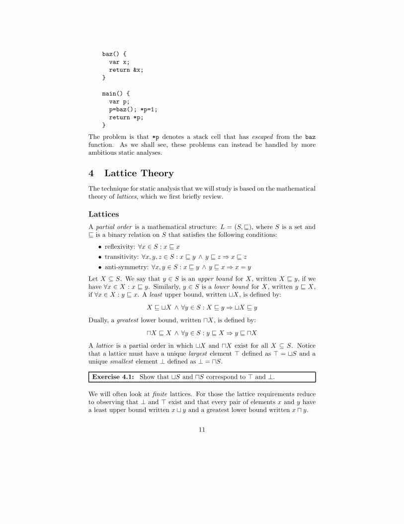
A finite partial order may be illustrated by a diagram in which the elementsare nodes and the order relation is the transitive closure of edges leading fromlower to higher nodes. With this notation, all of the following partial orders arealso lattices:
whereas these partial orders are not lattices:
Exercise 4.2: Why do these two diagrams not define lattices?
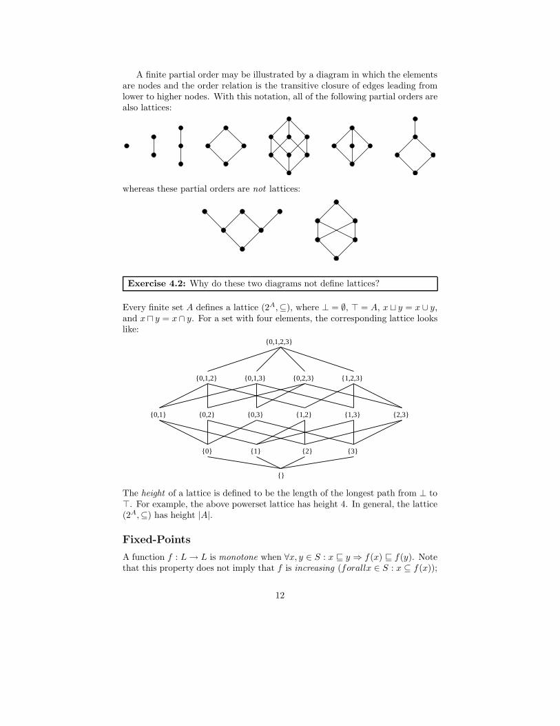
Every finite set A defines a lattice (2A,⊆), where ⊥ = ∅, ⊤ = A, x ⊔ y = x ∪ y,and x⊓ y = x∩ y. For a set with four elements, the corresponding lattice lookslike:
{0,1}
{0} {1}
{}
{2} {3}
{1,3} {2,3}{1,2}{0,3}{0,2}
{0,1,2} {0,1,3} {0,2,3} {1,2,3}
{0,1,2,3}
The height of a lattice is defined to be the length of the longest path from ⊥ to⊤. For example, the above powerset lattice has height 4. In general, the lattice(2A,⊆) has height |A|.
Fixed-Points
A function f : L→ L is monotone when ∀x, y ∈ S : x ⊑ y ⇒ f(x) ⊑ f(y). Notethat this property does not imply that f is increasing (forallx ∈ S : x ⊆ f(x));
12
for example, all constant functions are monotone. Viewed as functions ⊔ and⊓ are monotone in both arguments. Note that the composition of monotonefunctions is again monotone.
The central result we need is the fixed-point theorem. In a lattice L withfinite height, every monotone function f has a unique least fixed-point definedas:
fix(f) =⊔
i≥0
f i(⊥)
for which f(fix(f)) = fix(f). The proof of this theorem is quite simple. Observethat ⊥ ⊑ f(⊥) since ⊥ is the least element. Since f is monotone, it follows thatf(⊥) ⊑ f2(⊥) and by induction that f i(⊥) ⊑ f i+1(⊥). Thus, we have anincreasing chain:
⊥ ⊑ f(⊥) ⊑ f2(⊥) ⊑ . . .
Since L is assumed to have finite height, we must for some k have that fk(⊥) =fk+1(⊥). We define fix(f) = fk(⊥) and since f(fix(f)) = fk+1(⊥) = fk(⊥) =fix(f), we know that fix (f) is a fixed-point. Assume now that x is anotherfixed-point. Since ⊥ ⊑ x it follows that f(⊥) ⊑ f(x) = x, since f is monotoneand by induction we get that fix(f) = fk(⊥) ⊑ x. Hence, fix(f) is the leastfixed-point. By anti-symmetry, it is also unique.
The time complexity of computing a fixed-point depends on three factors:
• the height of the lattice, since this provides a bound for k;
• the cost of computing f ;
• the cost of testing equality.
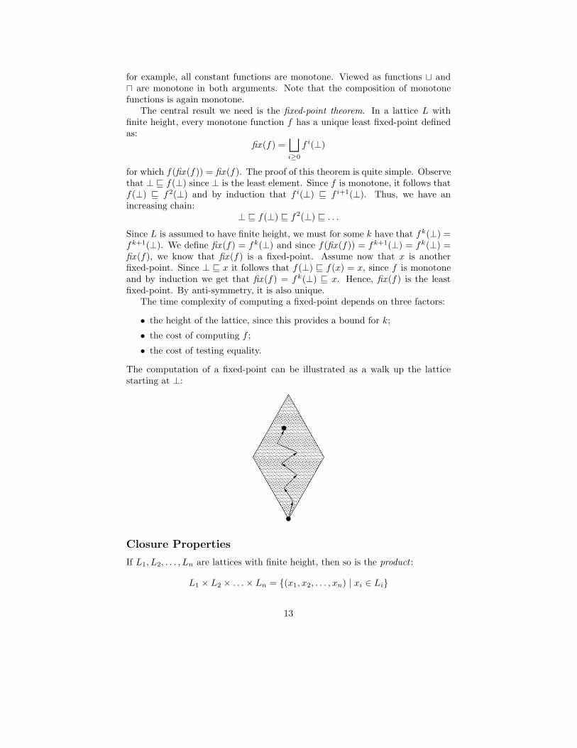
The computation of a fixed-point can be illustrated as a walk up the latticestarting at ⊥:
����������������������������������������������������������������������������������������������������������������������������������������������������������������������������������������������������������������������������������������������������������������������������������������������������������������������������������������������������������������������������������
����������������������������������������������������������������������������������������������������������������������������������������������������������������������������������������������������������������������������������������������������������������������������������������������������������������������������������������������������������������������������������
Closure Properties
If L1, L2, . . . , Ln are lattices with finite height, then so is the product :
L1 × L2 × . . .× Ln = {(x1, x2, . . . , xn) | xi ∈ Li}
13
where ⊑ is defined pointwise. Note that ⊔ and ⊓ can be computed pointwiseand that height(L1 × . . .×Ln) = height(L1) + . . .+ height(Ln). There is also asum operator:
L1 + L2 + . . .+ Ln = {(i, xi) | xi ∈ Li\{⊥,⊤}} ∪ {⊥,⊤}
where ⊥ and ⊤ are as expected and (i, x) ⊑ (j, y) if and only if i = j and x ⊑ y.Note that height(L1 + . . .+ Ln) = max{height(Li)}. The sum operator can beillustrated as follows:
������������������������������������������������������������������������������������������������������������������������
������������������������������������������������������������������������������������������������������������������������
������������������������������������������������
������������������������������������������������
������������������������������������������������������������������������������������������������������������������������������������������������������������������������
������������������������������������������������������������������������������������������������������������������������������������������������������������������������
��
��
...
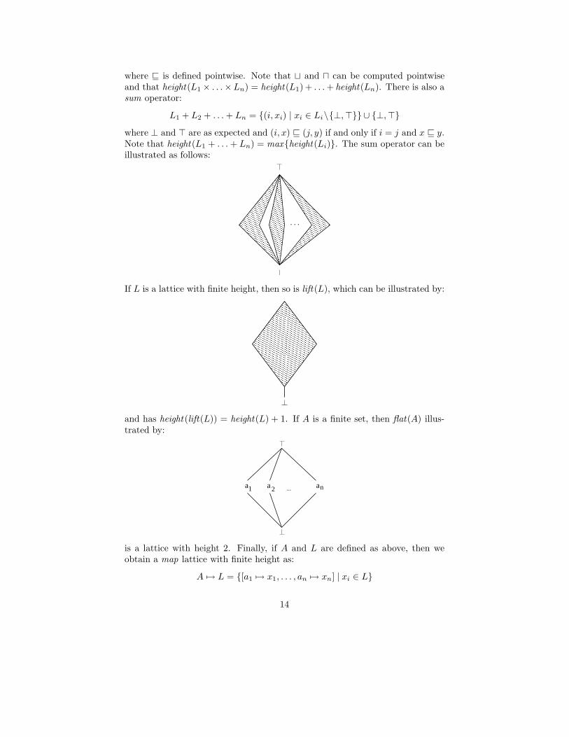
If L is a lattice with finite height, then so is lift(L), which can be illustrated by:
������������������������������������������������������������������������������������������������������������������������������������������������������������������������
������������������������������������������������������������������������������������������������������������������������������������������������������������������������
��
and has height (lift(L)) = height(L) + 1. If A is a finite set, then flat(A) illus-trated by:
a ...a a1 2 n
is a lattice with height 2. Finally, if A and L are defined as above, then weobtain a map lattice with finite height as:
A 7→ L = {[a1 7→ x1, . . . , an 7→ xn] | xi ∈ L}
14
ordered pointwise: f ⊑ g ⇔ ∀ai : f(ai) ⊑ g(ai). Note that height(A 7→ L) =|A| · height(L).
Exercise 4.3: Verify the above claims about the heights of the lattices thatare constructed.
Equations and Inequations
Fixed-points are interesting because they allow us to solve systems of equations.Let L be a lattice with finite height. An equation system is of the form:
x1 = F1(x1, . . . , xn)x2 = F2(x1, . . . , xn)...xn = Fn(x1, . . . , xn)
where xi are variables and Fi : Ln → L is a collection of monotone functions.Every such system has a unique least solution, which is obtained as the leastfixed-point of the function F : Ln → Ln defined by:
F (x1, . . . , xn) = (F1(x1, . . . , xn), . . . , Fn(x1, . . . , xn))
We can similarly solve systems of inequations of the form:
x1 ⊑ F1(x1, . . . , xn)x2 ⊑ F2(x1, . . . , xn)...xn ⊑ Fn(x1, . . . , xn)
by observing that the relation x ⊑ y is equivalent to x = x⊓ y. Thus, solutionsare preserved by rewriting the system into:
x1 = x1 ⊓ F1(x1, . . . , xn)x2 = x2 ⊓ F2(x1, . . . , xn)...xn = xn ⊓ Fn(x1, . . . , xn)
which is just a system of equations with monotone functions as before.
Exercise 4.4: Show that x ⊑ y is equivalent to x = x ⊓ y.
5 Control Flow Graphs
Type analysis started with the syntax tree of a program and defined constraintsover variables assigned to nodes. Analyses that work in this manner are flow
15
insensitive, in the sense that the results remain the same if a statement sequenceS 1S 2 is permuted into S 2S 1. Analyses that are flow sensitive use a control flowgraph, which is a different representation of the program source.
For now, we consider only the subset of the TIP language consisting of asingle function body without pointers. A control flow graph (CFG) is a directedgraph, in which nodes correspond to program points and edges represent possibleflow of control. A CFG always has a single point of entry, denoted entry, and asingle point of exit, denoted exit.
If v is a node in a CFG then pred(v) denotes the set of predecessor nodesand succ(v) the set of successor nodes.
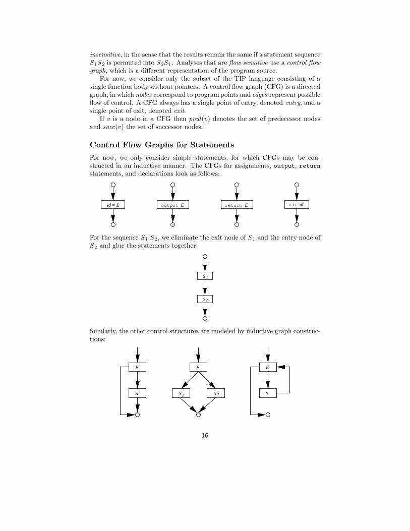
Control Flow Graphs for Statements
For now, we only consider simple statements, for which CFGs may be con-structed in an inductive manner. The CFGs for assignments, output, returnstatements, and declarations look as follows:
EreturnEoutputid = E var id
For the sequence S 1 S 2, we eliminate the exit node of S 1 and the entry node ofS 2 and glue the statements together:
S
S
1
2
Similarly, the other control structures are modeled by inductive graph construc-tions:
E
S S1 2
E
S
E
S
16
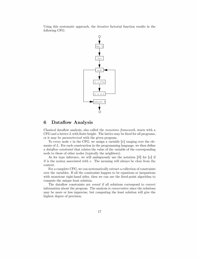
Using this systematic approach, the iterative factorial function results in thefollowing CFG:
f=1
n>0
n = n−1
f = f*n
var f
return f
6 Dataflow Analysis
Classical dataflow analysis, also called the monotone framework, starts with aCFG and a lattice L with finite height. The lattice may be fixed for all programs,or it may be parameterized with the given program.
To every node v in the CFG, we assign a variable [[v]] ranging over the ele-ments of L. For each construction in the programming language, we then definea dataflow constraint that relates the value of the variable of the correspondingnode to those of other nodes (typically the neighbors).
As for type inference, we will ambiguously use the notation [[S]] for [[v]] ifS is the syntax associated with v. The meaning will always be clear from thecontext.
For a complete CFG, we can systematically extract a collection of constraintsover the variables. If all the constraints happen to be equations or inequationswith monotone right-hand sides, then we can use the fixed-point algorithm tocompute the unique least solution.
The dataflow constraints are sound if all solutions correspond to correctinformation about the program. The analysis is conservative since the solutionsmay be more or less imprecise, but computing the least solution will give thehighest degree of precision.
17
Fixed-Point Algorithms
If the CFG has nodes V = {v1, v2, . . . , vn}, then we work in the lattice Ln.Assuming that node vi generates the dataflow equation [[vi]] = Fi([[v1]], . . . , [[vn]]),we construct the combined function F : Ln → Ln as described earlier:
F (x1, . . . , xn) = (F1(x1, . . . , xn), . . . , Fn(x1, . . . , xn))
The naive algorithm is then to proceed as follows:
x = (⊥, . . . ,⊥);do { t = x; x = F (x); }while (x 6= t);
to compute the fixed-point x. A better algorithm, called chaotic iteration,exploits the fact that our lattice has the structure Ln:
x1 = ⊥; . . .xn = ⊥;
do {t1 = x1; . . . tn = xn;
x1 = F1(x1, . . . , xn);. . .xn = Fn(x1, . . . , xn);
} while (x1 6= t1 ∨ . . . ∨ xn 6= tn);
to compute the fixed-point (x1, . . . , xn).
Exercise 6.1: Why is chaotic iteration better than the naive algorithm?
Both algorithms are, however, clearly wasteful since the information for allnodes is recomputed in every iteration, even though we may know that it cannothave changed. To obtain an even better algorithm, we must study further thestructure of the individual constraints.
In the general case, every variable [[vi]] depends on all other variables. Mostoften, however, an actual instance of Fi will only read the values of a few othervariables. We represent this information as a map:
dep : V → 2V
which for each node v tells us the subset of other nodes for which [[v]] occurs ina nontrivial manner on the right-hand side of their dataflow equations. That is,dep(v) is the set of nodes whose information may depend on the information ofv. Armed with this information, we can present the work-list algorithm:
18
x1 = ⊥; . . .xn = ⊥;
q = [v1, . . . , vn];while (q 6= []) {
assume q = [vi, . . .];y = Fi(x1, . . . , xn);q = q.tail();
if (y 6= xi) {
for (v ∈ dep(vi)) q.append(v);xi = y;
}
}
to compute the fixed-point (x1, . . . , xn). The worst-case complexity has notchanged, but in practice this algorithm saves much time.
Exercise 6.2: Give an invariant that is strong enough to prove the correct-ness of the work-list algorithm.
Further improvements are possible. It may be beneficial to handle in separateturns the strongly connected components of the graph induced by the dep map,and the queue could be changed into a priority queue allowing us to exploitdomain-specific knowledge about a particular dataflow problem.
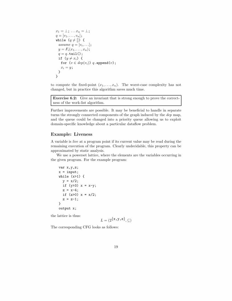
Example: Liveness
A variable is live at a program point if its current value may be read during theremaining execution of the program. Clearly undecidable, this property can beapproximated by static analysis.
We use a powerset lattice, where the elements are the variables occurring inthe given program. For the example program:
var x,y,z;
x = input;
while (x>1) {
y = x/2;
if (y>3) x = x-y;
z = x-4;
if (z>0) x = x/2;
z = z-1;
}
output x;
the lattice is thus:L = (2{x,y,z},⊆)
The corresponding CFG looks as follows:
19
z = x−4
z>0
z = z−1
output x
x = x−y
x = x/2
x = input x>1 y = x/2 y>3
var x,y,z
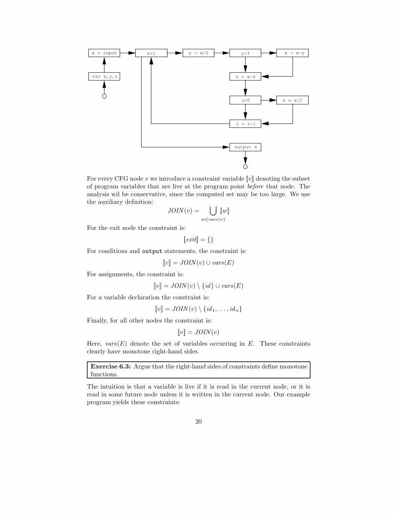
For every CFG node v we introduce a constraint variable [[v]] denoting the subsetof program variables that are live at the program point before that node. Theanalysis wil be conservative, since the computed set may be too large. We usethe auxiliary definition:
JOIN (v) =⋃
w∈succ(v)
[[w]]
For the exit node the constraint is:
[[exit]] = {}
For conditions and output statements, the constraint is:
[[v]] = JOIN (v) ∪ vars(E)
For assignments, the constraint is:
[[v]] = JOIN (v) \ {id} ∪ vars(E)
For a variable declaration the constraint is:
[[v]] = JOIN (v) \ {id1, . . . , idn}
Finally, for all other nodes the constraint is:
[[v]] = JOIN (v)
Here, vars(E) denote the set of variables occurring in E. These constraintsclearly have monotone right-hand sides.
Exercise 6.3: Argue that the right-hand sides of constraints define monotonefunctions.
The intuition is that a variable is live if it is read in the current node, or it isread in some future node unless it is written in the current node. Our exampleprogram yields these constraints:
20
[[var x,y,z;]] = [[x=input]] \ {x, y, z}[[x=input]] = [[x>1]] \ {x}[[x>1]] = ([[y=x/2]] ∪ [[output x]]) ∪ {x}[[y=x/2]] = ([[y>3]] \ {y}) ∪ {x}[[y>3]] = [[x=x-y]] ∪ [[z=x-4]] ∪ {y}[[x=x-y]] = ([[z=x-4]] \ {x}) ∪ {x,y}[[z=x-4]] = ([[z>0]] \ {z}) ∪ {x}[[z>0]] = [[x=x/2]] ∪ [[z=z-1]] ∪ {z}[[x=x/2]] = ([[z=z-1]] \ {x}) ∪ {x}[[z=z-1]] = ([[x>1]] \ {z}) ∪ {z}[[output x]] = [[exit ]] ∪ {x}[[exit ]] = {}
whose least solution is:
[[entry]] = {}[[var x,y,z;]] = {}[[x=input]] = {}[[x>1]] = {x}[[y=x/2]] = {x}[[y>3]] = {x, y}[[x=x-y]] = {x, y}[[z=x-4]] = {x}[[z>0]] = {x, z}[[x=x/2]] = {x, z}[[z=z-1]] = {x, z}[[output x]] = {x}[[exit ]] = {}
From this information a clever compiler could deduce that y and z are neverlive at the same time, and that the value written in the assignment z=z-1 isnever read. Thus, the program may safely be optimized into:
var x,yz;
x = input;
while (x>1) {
yz = x/2;
if (yz>3) x = x-yz;
yz = x-4;
if (yz>0) x = x/2;
}
output x;
which saves the cost of one assignment and could result in better register allo-cation.
We can estimate the worst-case complexity of this analysis. We first observethat if the program has n CFG nodes and k variables, then the lattice hasheight k ·n which bounds the number of iterations we can perform. Each lattice
21
element can be represented as a bitvector of length k. For each iteration wehave to perform O(n) intersection, difference, or equality operations which inall takes time O(kn). Thus, the total time complexity is O(k2n2).
Example: Available Expressions
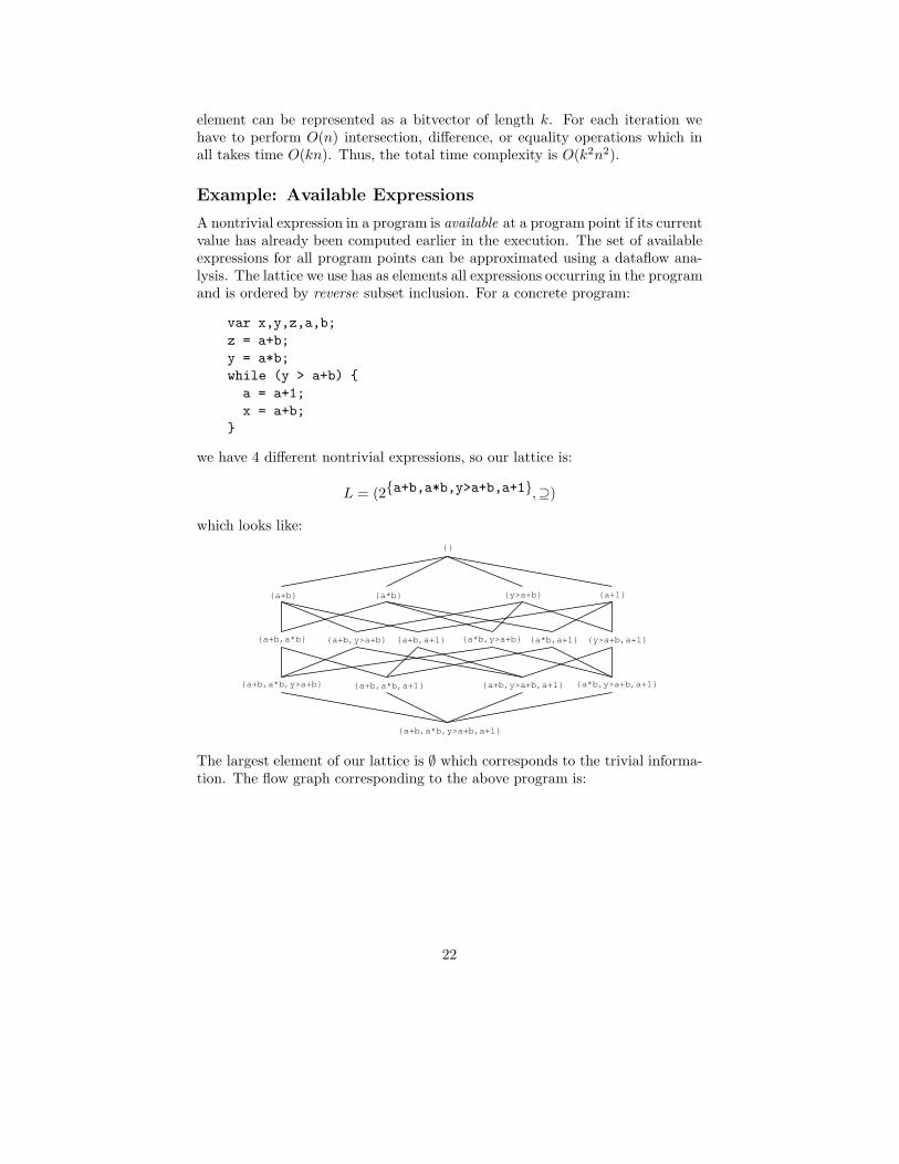
A nontrivial expression in a program is available at a program point if its currentvalue has already been computed earlier in the execution. The set of availableexpressions for all program points can be approximated using a dataflow ana-lysis. The lattice we use has as elements all expressions occurring in the programand is ordered by reverse subset inclusion. For a concrete program:
var x,y,z,a,b;
z = a+b;
y = a*b;
while (y > a+b) {
a = a+1;
x = a+b;
}
we have 4 different nontrivial expressions, so our lattice is:
L = (2{a+b,a*b,y>a+b,a+1},⊇)
which looks like:
{a+b,a*b,y>a+b,a+1}
{a+b,a*b,y>a+b} {a+b,a*b,a+1} {a+b,y>a+b,a+1} {a*b,y>a+b,a+1}
{a+b,a*b} {a+b,y>a+b} {a+b,a+1} {a*b,y>a+b} {a*b,a+1} {y>a+b,a+1}
{a+b} {a*b} {y>a+b} {a+1}
{}
The largest element of our lattice is ∅ which corresponds to the trivial informa-tion. The flow graph corresponding to the above program is:
22

z = a+b
y > a+b
a = a+1
x = a+b
y = a*b
var x,y,z,a,b
For each CFG node v we introduce a constraint variable [[v]] ranging over L. Ourintention is that it should contain the subset of expressions that are guaranteedalways to be available at the program point after that node. For example, theexpression a+b is available at the condition in the loop, but it is not availableat the final assignment in the loop. Our analysis will be conservative since thecomputed set may be too small. The dataflow constraints are defined as follows,where we this time define:
JOIN (v) =⋂
w∈pred(v)
[[w]]
For the entry node we have the constraint:
[[entry]] = {}
If v contains a condition E or the statement output E, then the constraint is:
[[v]] = JOIN (v) ∪ exps(E )
If v contains an assignment of the form id=E, then the constraint is:
[[v]] = (JOIN (v) ∪ exps(E ))↓ id
For all other kinds of nodes, the constraint is just:
[[v]] = JOIN (v)
Here the function ↓id removes all expressions that contain a reference to thevariable id, and the exps function is defined as:
23
exps(intconst) = ∅exps(id) = ∅exps(input) = ∅exps(E1opE2) = {E1opE2} ∪ exps(E1) ∪ exps(E2)
where op is any binary operator. The intuition is that an expression is availablein v if it is available from all incoming edges or is computed in v, unless itsvalue is destroyed by an assignment statement. Again, the right-hand sidesof the constraints are monotone functions. For the example program, we thengenerate the following concrete constraints:
[[entry]] = {}[[var x,y,z,a,b;]] = [[entry]][[z=a+b]] = exps(a+b) ↓z[[y=a*b]] = ([[z=a+b]] ∪ exps(a*b)) ↓y[[y>a+b]] = ([[y=a*b]] ∩ [[x=a+b]]) ∪ exps(y>a+b)[[a=a+1]] = ([[y>a+b]] ∪ exps(a+1))↓a[[x=a+b]] = ([[a=a+1]] ∪ exps(a+b))↓x[[exit ]] = [[y>a+b]]
Using the fixed-point algorithm, we obtain the minimal solution:
[[entry]] = {}[[var x,y,z,a,b;]] = {}[[z=a+b]] = {a+b}[[y=a*b]] = {a+b, a*b}[[y>a+b]] = {a+b, y>a+b}[[a=a+1]] = {}[[x=a+b]] = {a+b}[[exit ]] = {a+b}
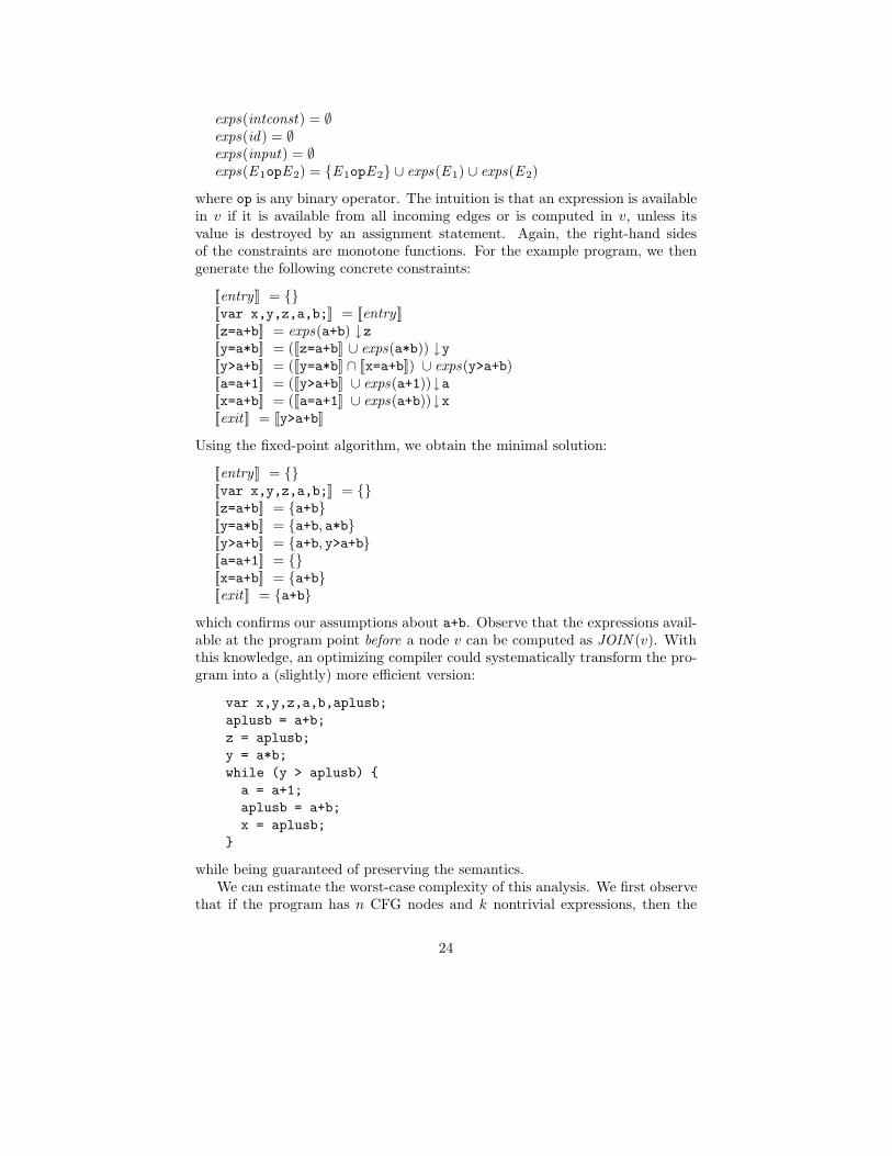
which confirms our assumptions about a+b. Observe that the expressions avail-able at the program point before a node v can be computed as JOIN (v). Withthis knowledge, an optimizing compiler could systematically transform the pro-gram into a (slightly) more efficient version:
var x,y,z,a,b,aplusb;
aplusb = a+b;
z = aplusb;
y = a*b;
while (y > aplusb) {
a = a+1;
aplusb = a+b;
x = aplusb;
}
while being guaranteed of preserving the semantics.We can estimate the worst-case complexity of this analysis. We first observe
that if the program has n CFG nodes and k nontrivial expressions, then the
24
lattice has height k ·n which bounds the number of iterations we perform. Eachlattice element can be represented as a bitvector of length k. For each iterationwe have to perform O(n) intersection, union, or equality operations which in alltakes time O(kn). Thus, the total time complexity is O(k2n2).
Example: Very Busy Expressions
An expression is very busy if it will definitely be evaluated again before itsvalue changes. To approximate this property, we need the same lattice andauxiliary functions as for available expressions. For every CFG node v thevariable [[v]] denotes the set of expressions that at the program point before thenode definitely are busy. We define:
JOIN (v) =⋂
w∈succ(v)
[[w]]
The constraint for the exit node is:
[[exit ]] = {}
For conditions and output statements we have:
[[v]] = JOIN (v) ∪ exps(E)
For assignments the constraint is:
[[v]] = JOIN (v) ↓ id ∪ exps(E)
For all other nodes we have the constraint:
[[v]] = JOIN (v)
The intuition is that an expression is very busy if it is evaluated in the currentnode or will be evaluated in all future executions unless an assignment changesits value. On the example program:
var x,a,b;
x = input;
a = x-1;
b = x-2;
while (x>0) {
output a*b-x;
x = x-1;
}
output a*b;
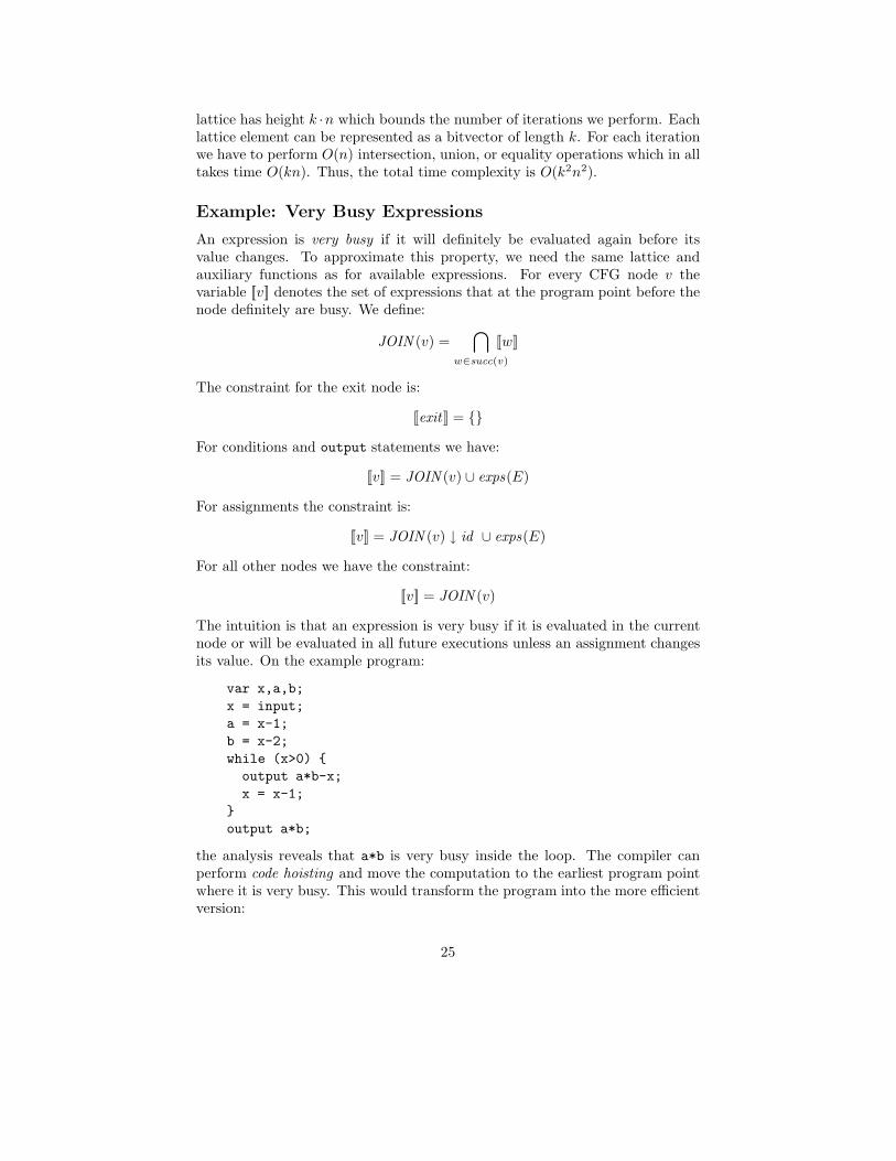
the analysis reveals that a*b is very busy inside the loop. The compiler canperform code hoisting and move the computation to the earliest program pointwhere it is very busy. This would transform the program into the more efficientversion:
25
var x,a,b,atimesb;
x = input;
a = x-1;
b = x-2;
atimesb = a*b;
while (x>0) {
output atimesb-x;
x = x-1;
}
output atimesb;
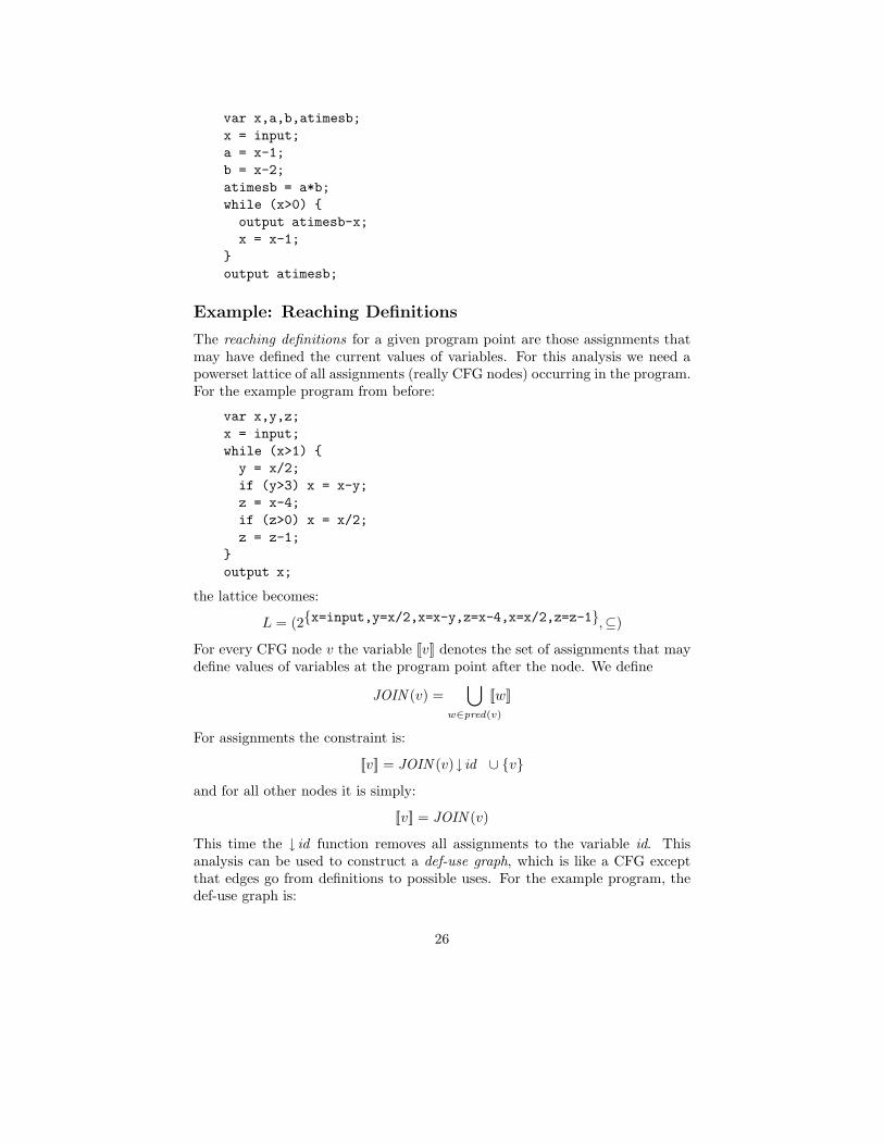
Example: Reaching Definitions
The reaching definitions for a given program point are those assignments thatmay have defined the current values of variables. For this analysis we need apowerset lattice of all assignments (really CFG nodes) occurring in the program.For the example program from before:
var x,y,z;
x = input;
while (x>1) {
y = x/2;
if (y>3) x = x-y;
z = x-4;
if (z>0) x = x/2;
z = z-1;
}
output x;
the lattice becomes:
L = (2{x=input,y=x/2,x=x-y,z=x-4,x=x/2,z=z-1},⊆)
For every CFG node v the variable [[v]] denotes the set of assignments that maydefine values of variables at the program point after the node. We define
JOIN (v) =⋃
w∈pred(v)
[[w]]
For assignments the constraint is:
[[v]] = JOIN (v)↓ id ∪ {v}
and for all other nodes it is simply:
[[v]] = JOIN (v)
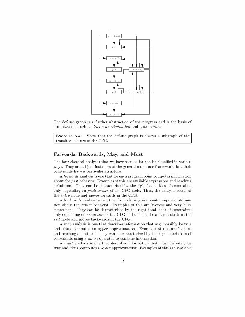
This time the ↓ id function removes all assignments to the variable id. Thisanalysis can be used to construct a def-use graph, which is like a CFG exceptthat edges go from definitions to possible uses. For the example program, thedef-use graph is:
26
x = input
x>1
y = x/2
y>3
z = x−4
z>0
z = z−1
output x
x = x−y
x = x/2
The def-use graph is a further abstraction of the program and is the basis ofoptimizations such as dead code elimination and code motion.
Exercise 6.4: Show that the def-use graph is always a subgraph of thetransitive closure of the CFG.
Forwards, Backwards, May, and Must
The four classical analyses that we have seen so far can be classified in variousways. They are all just instances of the general monotone framework, but theirconstraints have a particular structure.
A forwards analysis is one that for each program point computes informationabout the past behavior. Examples of this are available expressions and reachingdefinitions. They can be characterized by the right-hand sides of constraintsonly depending on predecessors of the CFG node. Thus, the analysis starts atthe entry node and moves forwards in the CFG.
A backwards analysis is one that for each program point computes informa-tion about the future behavior. Examples of this are liveness and very busyexpressions. They can be characterized by the right-hand sides of constraintsonly depending on successors of the CFG node. Thus, the analysis starts at theexit node and moves backwards in the CFG.
A may analysis is one that describes information that may possibly be trueand, thus, computes an upper approximation. Examples of this are livenessand reaching definitions. They can be characterized by the right-hand sides ofconstraints using a union operator to combine information.
A must analysis is one that describes information that must definitely betrue and, thus, computes a lower approximation. Examples of this are available
27
expressions and very busy expressions. They can be characterized by the right-hand sides of constraints using an intersection operator to combine information.
Thus, our four examples show every possible combination, as illustrated bythis diagram:
Forwards BackwardsMay Reaching Definitions LivenessMust Available Expressions Very Busy Expressions
These classifications are mostly botanical in nature, but awareness of them mayprovide inspiration for constructing new analyses.
Example: Initialized Variables
Let us try to define an analysis that ensures that variables are initialized beforethey are read. This can be solved by computing for every program point the setof variables that is guaranteed to be initialized, thus our lattice is the powersetof variables occurring in the given program. Initialization is a property of thepast, so we need a forwards analysis. Also, we need definite information whichimplies a must analysis. This means that our constraints are phrased in terms ofpredecessors and intersections. On this basis, they more or less give themselves.For the entry node we have the constraint:
[[entry ]] = {}
for assignments we have the constraint:
[[v]] =⋂
w∈pred(v)
[[w]] ∪ {id}
and for all other nodes the constraint:
[[v]] =⋂
w∈pred(v)
[[w]]
The compiler could now check for every use of a variable that it is contained inthe computed set of initialized variables.
Example: Sign Analysis
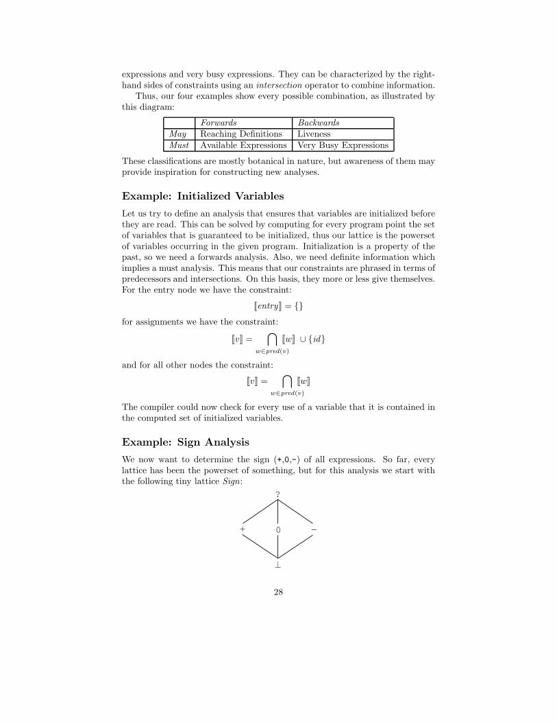
We now want to determine the sign (+,0,-) of all expressions. So far, everylattice has been the powerset of something, but for this analysis we start withthe following tiny lattice Sign:
?
+ 0 −
28

Here, ? denotes that the sign value is not constant and ⊥ denotes that the valueis unknown. The full lattice for our analysis is the map lattice:
Vars 7→ Sign
where Vars is the set of variables occurring in the given program. For eachCFG node v we assign a variable [[v]] that denotes a symbol table giving thesign values for all variables at the program point before the node. The dataflowconstraints are more involved this time. For variable declarations we updateaccordingly:
[[v]] = JOIN (v) [id1 7→ ?, . . . , idn 7→ ?]
For an assignment we use the constraint:
[[v]] = JOIN (v) [id 7→ eval (JOIN (v), E)]
and for all other nodes the constraint:
[[v]] = JOIN (v)
where:JOIN (v) =
⊔
w∈pred(v)
[[w]]
and eval performs an abstract evaluation of expressions:
eval (σ, id ) = σ(id )eval (σ, intconst) = sign(intconst)eval (σ,E1 opE2) = op(eval (σ,E1), eval(σ,E2))
where σ is the current environment, sign gives the sign of an integer constantand op is an abstract evaluation of the given operator, defined by the followingcollection of tables:
+ ⊥ 0 - + ?
⊥ ⊥ ⊥ ⊥ ⊥ ⊥
0 ⊥ 0 - + ?
- ⊥ - - ? ?
+ ⊥ + ? + ?
? ⊥ ? ? ? ?
- ⊥ 0 - + ?
⊥ ⊥ ⊥ ⊥ ⊥ ⊥
0 ⊥ 0 + - ?
- ⊥ - ? - ?
+ ⊥ + + ? ?
? ⊥ ? ? ? ?
* ⊥ 0 - + ?
⊥ ⊥ 0 ⊥ ⊥ ⊥
0 0 0 0 0 0
- ⊥ 0 + - ?
+ ⊥ 0 - + ?
? ⊥ 0 ? ? ?
/ ⊥ 0 - + ?
⊥ ⊥ ⊥ ⊥ ⊥ ⊥
0 ⊥ ? 0 0 ?
- ⊥ ? ? ? ?
+ ⊥ ? ? ? ?
? ⊥ ? ? ? ?
29

> ⊥ 0 - + ?
⊥ ⊥ ⊥ ⊥ ⊥ ⊥
0 ⊥ 0 + 0 ?
- ⊥ 0 ? 0 ?
+ ⊥ + + ? ?
? ⊥ ? ? ? ?
== ⊥ 0 - + ?
⊥ ⊥ ⊥ ⊥ ⊥ ⊥
0 ⊥ + 0 0 ?
- ⊥ 0 ? 0 ?
+ ⊥ 0 0 ? ?
? ⊥ ? ? ? ?
It is not obvious that the right-hand sides of our constraints correspond tomonotone functions. However, the ⊔ operator and map updates clearly are, soit all comes down to monotonicity of the abstract operators on the sign lattice.This is best verified by a tedious manual inspection. Notice that for a latticewith n elements, monotonicity of an n × n table can be verified automaticallyin time O(n3).
Exercise 6.5: Describe the O(n3) algorithm for checking monotonicity ofan operator given by an n× n table.
Exercise 6.6: Check that the above tables indeed define monotone operatorson the Sign lattice.
We lose some information in the above analysis, since for example the expression(2>0)==1 is analyzed as ?, which seems unnecessarily coarse. Also, +/+ resultsin ? rather than + since e.g. 1/2 is rounded down to zero. To handle thesesituations more precisely, we could enrich the sign lattice with element 1 (theconstant 1), +0 (positive or zero), and -0 (negative or zero) to keep track ofmore precise abstract values:
?
1
+ 0 −
+0 −0
30
and consequently describe the abstract operators by 8 × 8 tables.
Exercise 6.7: Define the six operators on the extended Sign lattice bymeans of 8 × 8 tables. Check that they are properly monotone.
The results of a sign analysis could in theory be used to eliminate division byzero errors by only accepting programs in which denominator expressions havesign +, -, or 1. However, the resulting analysis will probably unfairly reject toomany programs to be practical.
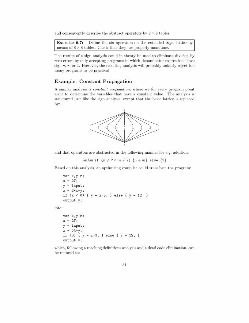
Example: Constant Propagation
A similar analysis is constant propagation, where we for every program pointwant to determine the variables that have a constant value. The analysis isstructured just like the sign analysis, except that the basic lattice is replacedby:
0 1 2 3−3 −2 −1
?
and that operators are abstracted in the following manner for e.g. addition:
λnλm.if (n 6= ? ∧m 6= ?) {n+m} else {?}
Based on this analysis, an optimizing compiler could transform the program:
var x,y,z;
x = 27;
y = input;
z = 2*x+y;
if (x < 0) { y = z-3; } else { y = 12; }
output y;
into:
var x,y,z;
x = 27;
y = input;
z = 54+y;
if (0) { y = z-3; } else { y = 12; }
output y;
which, following a reaching definitions analysis and a dead code elimination, canbe reduced to:
31
var y;
y = input;
output 12;
7 Widening and Narrowing
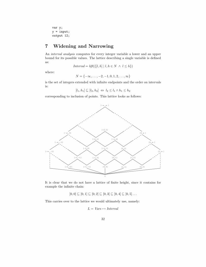
An interval analysis computes for every integer variable a lower and an upperbound for its possible values. The lattice describing a single variable is definedas:
Interval = lift({[l, h] | l, h ∈ N ∧ l ≤ h})
where:N = {−∞, . . . ,−2,−1, 0, 1, 2, . . . ,∞}
is the set of integers extended with infinite endpoints and the order on intervalsis:
[l1, h1] ⊑ [l2, h2] ⇔ l2 ≤ l1 ∧ h1 ≤ h2
corresponding to inclusion of points. This lattice looks as follows:
[−2,−2] [−1,−1] [0,0] [1,1] [2,2]
[1,2][0,1][−1,0]
[− ,−2]
[− ,−1]
[− ,0]
[−2,0] [−1,1] [0,2]
[2, ]
[1, ]
[−2,2]
[−2,1] [−1,2]
[− , ]8 8
8
8
8
8
8
8
[0, ]
[−2,−1]
It is clear that we do not have a lattice of finite height, since it contains forexample the infinite chain:
[0, 0] ⊑ [0, 1] ⊑ [0, 2] ⊑ [0, 3] ⊑ [0, 4] ⊑ [0, 5] . . .
This carries over to the lattice we would ultimately use, namely:
L = Vars 7→ Interval
32
where for the entry node we use the constant function returning the ⊤ element:
[[entry]] = λx.[−∞,∞]
for an assignment the constraint:
[[v]] = JOIN (v) [id 7→ eval (JOIN (v), E)]
and for all other nodes the constraint:
[[v]] = JOIN (v)
where:JOIN (v) =
⊔
w∈pred(v)
[[w]]
and eval performs an abstract evaluation of expressions:
eval (σ, id ) = σ(id )eval (σ, intconst) = [intconst , intconst ]eval (σ,E1 opE2) = op(eval (σ,E1), eval(σ,E2))
where the abstract operators all are defined by:
op([l1, h1], [l2, h2]) = [ minx∈[l1,h1],y∈[l2,h2]
x op y, maxx∈[l1,h1],y∈[l2,h2]
x op y]
For example, +([1, 10], [−5, 7]) = [1 − 5, 10 + 7] = [−4, 17].
Exercise 7.1: Argue that these definitions yield monotone operators on theInterval lattice.
The lattice has infinite height, so we are unable to use the monotone framework,since the fixed-point algorithm may never terminate. This means that for thelattice Ln the sequence of approximants:
F i(⊥, . . . ,⊥)
need never converge. Instead of giving up, we shall use a technique calledwidening which introduces a function w : Ln → Ln so that the sequence:
(w ◦ F )i(⊥, . . . ,⊥)
now converges on a fixed-point that is larger than every F i(⊥, . . . ,⊥) and thusrepresents sound information about the program. The widening function w willintuitively coarsen the information sufficiently to ensure termination. For ourinterval analysis, w is defined pointwise down to single intervals. It operatesrelatively to a fixed finite subset B ⊂ N that must contain −∞ and ∞. Typ-ically, B could be seeded with all the integer constants occurring in the givenprogram, but other heuristics could also be used. On a single interval we have:
w([l, h]) = [max{i ∈ B | i ≤ l},min{i ∈ B | h ≤ i}]
33
which finds the best fitting interval among the ones that are allowed.
Exercise 7.2: Show that since w is an increasing monotone function andw(Interval) is a finite lattice, the widening technique is guaranteed to workcorrectly.
Widening shoots above the target, but a subsequent technique called narrowingmay improve the result. If we define:
fix =⊔
F i(⊥, . . . ,⊥) fixw =⊔
(w ◦ F )i(⊥, . . . ,⊥)
then we have fix ⊑ fixw . However, we also have that fix ⊑ F (fixw) ⊑ fixw ,which means that a subsequent application of F may refine our result and stillproduce sound information. This technique, called narrowing, may in fact beiterated arbitrarily many times.
Exercise 7.3: Show that fix ⊑ F i+1(fixw) ⊑ F i(fixw) ⊑ fixw .
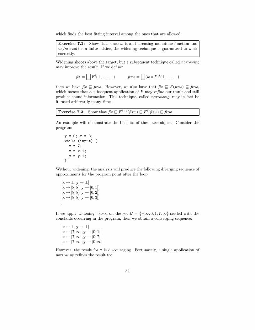
An example will demonstrate the benefits of these techniques. Consider theprogram:
y = 0; x = 8;
while (input) {
x = 7;
x = x+1;
y = y+1;
}
Without widening, the analysis will produce the following diverging sequence ofapproximants for the program point after the loop:
[x 7→ ⊥, y 7→ ⊥][x 7→ [8, 8], y 7→ [0, 1]][x 7→ [8, 8], y 7→ [0, 2]][x 7→ [8, 8], y 7→ [0, 3]]...
If we apply widening, based on the set B = {−∞, 0, 1, 7,∞} seeded with theconstants occurring in the program, then we obtain a converging sequence:
[x 7→ ⊥, y 7→ ⊥][x 7→ [7,∞], y 7→ [0, 1]][x 7→ [7,∞], y 7→ [0, 7]][x 7→ [7,∞], y 7→ [0,∞]]
However, the result for x is discouraging. Fortunately, a single application ofnarrowing refines the result to:
34
[x 7→ [8, 8], y 7→ [0,∞]]
which is really the best we could hope for. Correspondingly, further narrowinghas no effect. Note that the decreasing sequence:
fixw ⊒ F (fixw) ⊒ F 2(fixw) ⊒ F 3(fixw) . . .
is not guaranteed to converge, so heuristics must determine how many times toapply narrowing.
8 Conditions and Assertions
Until now, we have ignored the values of conditions by simply treating if- andwhile-statements as a nondeterministic choice between the two branches. Thistechnique fails to include some information that could potentially be used in astatic analysis. Consider for example the following program:
x = input;
y = 0;
z = 0;
while (x > 0) {
z = z+x;
if (17 > y) { y = y+1; }
x = x-1;
}
The previous interval analysis (with widening) will conclude that after thewhile-loop the variable x is in the interval [−∞,∞], y is in the interval [0,∞],and z is in the interval [−∞,∞]. However, in view of the conditionals beingused, this result seems too pessimistic.
To exploit the available information, we shall extend the language with twoartificial statements: assert(E) and refute(E), where E is a condition fromour base language. In the interval analysis, the constraints for these new state-ment will narrow the intervals for the various variables by exploiting the infor-mation that E must be true respectively false.
The meanings of the conditionals are then encoded by the following programtransformation:
x = input;
y = 0;
z = 0;
while (x > 0) {
assert(x > 0);
z = z+x;
if (17 > y) { assert(17 > y); y = y+1; }
x = x-1;
}
refute(x > 0);
35

Constraints for a node v with an assert or refute statement may trivially begiven as:
[[v]] = JOIN (v)
in which case no extra precision is gained. In fact, it requires insight intothe specific static analysis to define non-trivial and sound constraints for theseconstructs.
For the interval analysis, extracting the information carried by general con-ditions such as E1 > E2 or E1 == E2 is complicated and in itself an area ofconsiderable study. For our purposes, we need only consider conditions of thetwo kinds id > E or E > id , the first of which for the case of assert can behandled by:
[[v]] = JOIN (v)[id 7→ gt(JOIN (v)(id ), eval(JOIN (v), E))]
where:gt([l1, h1], [l2, h2]) = [l1, h1] ⊓ [l2,∞]
The cases of refute and the dual condition are handled in similar fashions, andall other condtions are given the trivial, but sound identity constraint.
With this refinement, the interval analysis of the above example will concludethat after the while-loop the variable x is in the interval [−∞..0], y is in theinterval [0, 17], and z is in the interval [0,∞].
Exercise 8.1: Discuss how more conditions may be given non-trivial con-straints for assert and refute.
9 Interprocedural Analysis
So far, we have only analyzed the body of a single function, which is called anintraprocedural analysis. When we consider whole programs containing func-tion calls as well, the analysis is called interprocedural. The alternative to thistechnique is to analyze each function in isolation with maximally pessimisticassumptions about the results of function calls.
Flow Graphs for Programs
We now consider the subset of the TIP language containing functions, but stillignore pointers. The CFG for an entire program is actually quite simple toobtain, since it corresponds to the CFG for a simple program that can be sys-tematically obtained.
First we construct the CFGs for all individual function bodies. All thatremains is then to glue them together to reflect function calls properly. Thistask is made simpler by the fact that we assume all declared identifiers to beunique.
36
We start by introducing a collection of shadow variables. For every functionf we introduce the variable ret-f, which corresponds to its return value. Forevery call site we introduce a variable call-i, where i is a unique index, whichdenotes the value computed by that function call. For every local variable orformal argument named x in the calling function and every call site, we introducea variable save-i-x to preserve its value across that function call. Finally, forevery formal argument named x in the called function and every call site, weintroduce a temporary variable temp-i-x.
For simplicity we assume that all function calls are performed in connectionwith assignments:
x = f(E1,. . . ,,En);
Exercise 9.1: Show how any program can be rewritten to have this formby introducing new temporary variables.
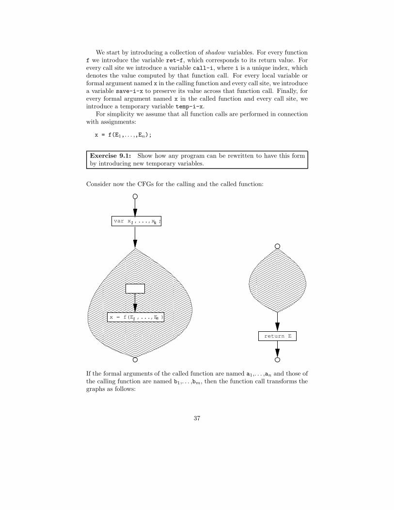
Consider now the CFGs for the calling and the called function:
������������������������������������������������������������������������������������������������������������������������������������������������������������������������������������������������������������������
������������������������������������������������������������������������������������������������������������������������������������������������������������������������������������������������������������������
������������������������������������������������������������������������������������������������������������������������������������������������������������������������������������������������������������������������������������������������
������������������������������������������������������������������������������������������������������������������������������������������������������������������������������������������������������������������������������������������������
������������������������������������������������������������������������
������������������������������������������������������������������������
������������������������������������������������������������������������
������������������������������������������������������������������������
x = f(E ,...,E )
return E
n1
kvar x ,...,x ;1
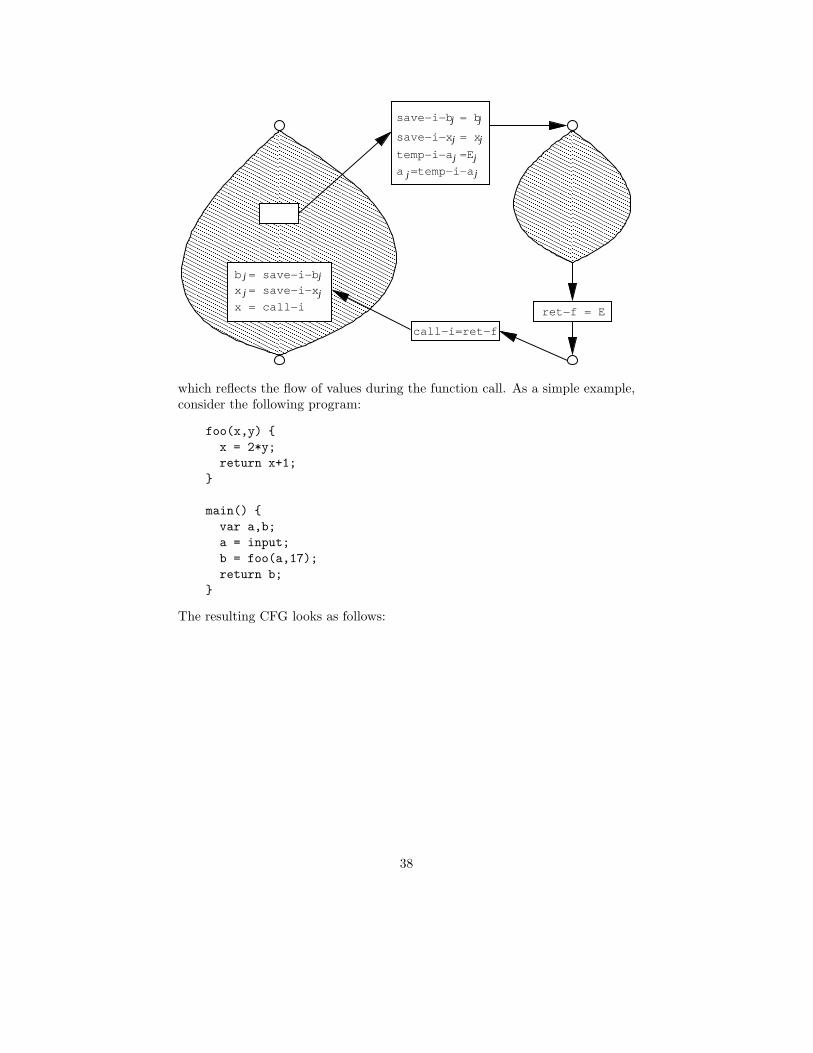
If the formal arguments of the called function are named a1,. . . ,an and those ofthe calling function are named b1,. . . ,bm, then the function call transforms thegraphs as follows:
37
������������������������������������������������������������������������������������������������������������������������������������������������������������������������������������������������������������������
������������������������������������������������������������������������������������������������������������������������������������������������������������������������������������������������������������������
������������������������������������������������������������������������������������������������������������������������������������������������������������������������������������������������������������������������������������������������
������������������������������������������������������������������������������������������������������������������������������������������������������������������������������������������������������������������������������������������������
������������������������������������������������������������������������
������������������������������������������������������������������������
������������������������������������������������������������������������
������������������������������������������������������������������������
call−i=ret−f
ret−f = E
save−i−b = bj j
j j
b = save−i−b
x = save−i−x
x = call−i
j j
j j
temp−i−a =E
a =temp−i−aj j
jj
save−i−x = x
which reflects the flow of values during the function call. As a simple example,consider the following program:
foo(x,y) {
x = 2*y;
return x+1;
}
main() {
var a,b;
a = input;
b = foo(a,17);
return b;
}
The resulting CFG looks as follows:
38

call−1=ret−foo
ret−main=b
b = call−1
b = save−1−b
a = save−1−a
save−1−b = b
save−1−a = a
temp−1−x = a
temp−1−y = 17
x = temp−1−x
y = temp−1−y
x = 2*y
ret−foo=x+1
var a,b
a = input
and can now be analyzed using the standard monotone framework. Note howthis construction implies that function arguments are evaluated from left toright. In future examples, the temporary variables will only be used whennecessary.
Exercise 9.2: How many edges may the interprocedural CFG contain?
Polyvariance
The interprocedural analysis we have presented so far is called monovariant,since each function body is represented only once for every call site. A poly-variant analysis will perform context-dependent analysis of function calls. Asan example, consider the following program:
foo(a) {
return a;
}
bar() { baz() {
var x; var y;
x = foo(17); y = foo(18);
return x; return y;
} }
which is modeled by this CFG:
39

a = 17 a = 18
call−1=ret−foo
ret−bar=x ret−baz=y
x = call−1 y = call−2
x = save−1−x y = save−2−y
call−2=ret−fooret−foo=a
save−1−x = x save−2−y = y
var x var y
If we subsequently perform a constant propagation analysis, then the returnvalues from both bar and baz are deemed to be non-constant. The problem isthat the CFG merges both calls to foo.
The analysis can be made polyvariant by creating multiple copies of the CFGfor the body of the called function. There are numerous strategies for decidinghow many copies to create. The simplest is to create one copy for every callsite, which handles the above problem with constant propagation:
a = 17
call−1=ret−foo
ret−bar=x
x = call−1
x = save−1−x
ret−foo=a
save−1−x = x
a = 18
ret−baz=y
y = call−2
y = save−2−y
call−2=ret−foo
save−2−y = y
ret−foo=a
var x var y
If, however, the call to foo was wrapped in a further layer of function calls,then nothing would have been gained. Similarly, recursive functions are notbenefited much by this technique. The best approach is to employ heuristicsthat are specific to the intended analysis. It is of course important to ensurethat only finitely many copies can be created.
Example: Tree Shaking
An example of an interprocedural analysis is tree shaking, where we want toidentify those functions that are never called and safely can be removed from theprogram. This is particularly useful if the program is being compiled togetherwith a large function library.
The analysis takes place on the monovariant interprocedural CFG but isotherwise phrased just like the other analyses we have seen. The lattice is the
40
powerset of function names occurring in the given program, and for every CFGnode v we introduce a constraint variable [[v]] denoting the set of functions thatcould possibly be called in the future. We use the notation entry(id) for theentry node of the function named id. For assignments, conditions, and output
statements the constraint is:
[[v]] =⋃
w∈succ(v)
[[w]] ∪ funcs(E) ∪⋃
f∈funcs(E)
[[entry(f)]]
and for all other nodes just:
[[v]] =⋃
w∈succ(v)
[[w]]
where funcs is defined as:
funcs(id) = funcs(intconst) = funcs(input) = ∅funcs(E1 opE2) = funcs(E1) ∪ funcs(E2)funcs(id(E1, . . . , En)) = {id} ∪ funcs(E1) ∪ . . . ∪ funcs(En)
As usual, these constraints can be seen to be monotone. Every function that isnot mentioned in the resulting value of [[entry(main)]] is guaranteed to be dead.
10 Control Flow Analysis
Interprocedural analysis is fairly straightforward in a language with only first-order functions. If we introduce higher-order functions, objects, or functionpointers, then control flow and dataflow suddenly becomes intertwined. Thetask of control flow analysis is to approximate conservatively the control flowgraph for such languages.
Closure Analysis for the λ-calculus
Control flow analysis in its purest form can best be illustrated by the classicalλ-calculus:
E → λid.E→ id→ E E
and later we shall generalize this technique to the full TIP language. For sim-plicity we assume that all λ-bound variables are distinct. To construct a CFGfor a term in this calculus, we need to compute for every expression E the setof closures to which it may evaluate. A closure is in our setting a symbol of theform λid that identifies a concrete λ-abstraction. This problem, called closureanalysis, can be solved using a variation of the monotone framework. However,since the CFG is not available, the analysis will take place on the syntax tree.
41
The lattice we use is the powerset of closures occurring in the given termordered by subset inclusion. For every syntax tree node v we introduce a con-straint variable [[v]] denoting the set of resulting closures. For an abstractionλid.E we have the constraint:
{λid} ⊆ [[λid .E]]
(the function may certainly evaluate to itself) and for an application E1E2 theconditional constraint:
λid ∈ [[E1]] ⇒ [[E2]] ⊆ [[id ]] ∧ [[E]] ⊆ [[E1E2]]
for every closure λid.E (the actual argument may flow into the formal argumentand the value of the function body is among the possible results of the functioncall). Note that this is a flow insensitive analysis.
Exercise 10.1: Show how the resulting constraints can be transformed intostandard monotone inequations and solved by a fixed-point computation.
The Cubic Algorithm
The constraints for closure analysis are an instance of a general class that can besolved in cubic time. Many problems fall into this category, so we will investigatethe algorithm more closely.
We have a set of tokens {t1, . . . , tk} and a collection of variables x1, . . . , xn
whose values are subsets of token. Our task is to read a sequence of constraintsof the form {t}⊆x or t∈x ⇒ y⊆z and produce the minimal solution.
Exercise 10.2: Show that a unique minimal solution exists, since solutionsare closed under intersection.
The algorithm is based on a simple data structure. Each variable is mapped to anode in a directed acyclic graph (DAG). Each node has an associated bitvectorbelonging to {0, 1}k, initially defined to be all 0’s. Each bit has an associatedlist of pairs of variables, which is used to model conditional constraints. Theedges in the DAG reflect inclusion constraints. The bitvectors will at all timesdirectly represent the minimal solution. An example graph may look like:
42

x
x
x
x
(x ,x )2 4
1
4
3
2
Constraints are added one at a time. A constraint of the form {t} ⊆ x is handledby looking up the node associated with x and setting the corresponding bit to 1.If its list of pairs was not empty, then an edge between the nodes correspondingto y and z is added for every pair (y, z). A constraint of the form t ∈ x⇒ y ⊆ z
is handled by first testing if the bit corresponding to t in the node correspondingto x has value 1. If this is so, then an edge between the nodes corresponding toy and z is added. Otherwise, the pair (y, z) is added to the list for that bit.
If a newly added edge forms a cycle, then all nodes on that cycle are mergedinto a single node, which implies that their bitvectors are unioned together andtheir pair lists are concatenated. The map from variables to nodes is updatedaccordingly. In any case, to reestablish all inclusion relations we must propagatethe values of each newly set bit along all edges in the graph.
To analyze this algorithm, we assume that the numbers of tokens and con-straints are both O(n). This is clearly the case when analyzing programs, wherethe numbers of variables, tokens, and constraints all are linear in the size of theprogram.
Merging DAG nodes on cycles can be done at most O(n) times. Each mergerinvolves at most O(n) nodes and the union of their bitvectors is computed intime at most O(n2). The total for this part is O(n3).
New edges are inserted at most O(n2) times. Constant sets are included atmost O(n2) times, once for each {t} ⊆ x constraint.
Finally, to limit the cost of propagating bits along edges, we imagine thateach pair of corresponding bits along an edge are connected by a tiny bitwire.Whenever the source bit is set to 1, that value is propagated along the bitwirewhich then is broken:
1 1
0
0
0
0
1
0
0
1
0
1
Since we have at most n3 bitwires, the total cost for propagation is O(n3).
43

Adding up, the total cost for the algorithm is also O(n3). The fact that thisseems like a lower bound as well is referred to as the cubic time bottleneck.
The kinds of constraints covered by this algorithm is a simple case of themore general set constraints, which allows richer constraints on sets of finiteterms. General set constraints are also solvable but in time O(22n
).
Control Flow Graphs for Function Pointers
Consider now our tiny language where we allow functions pointers. For a com-puted function call:
E → (E)(E1,. . . ,En)
we cannot see from the syntax which functions may be called. A coarse butsound CFG could be obtained by assuming that any function with the rightnumber of arguments could be called. However, we can do much better byperforming a control flow analysis. Note that a function call id(E1,. . . ,En)
may be seen as syntactic sugar for the general notation (id)(E1,. . . ,En).Our lattice is the powerset of the set of tokens containing &id for every
function name id, ordered by subset inclusion. For every syntax tree node vwe introduce a constraint variable [[v]] denoting the set of functions or functionpointers to which v could evaluate. For a constant function name id we havethe constraint:
{&id} ⊆ [[id ]]
for assignments id=E we have the constraint:
[[E ]] ⊆ [[id ]]
and, finally, for computed function calls we have for every definition of a functionf with arguments a1, . . . , an and return expression E′ the constraint:
&f ∈ [[E]] ⇒ [[Ei]] ⊆ [[ai]] ∧ [[E′]] ⊆ [[(E)(E1, . . . ,En)]]
A still more precise analysis could be obtained if we restricted ourselves totypable programs and only generated constraints for those functions f for whichthe call would be type correct.
Given this inferred information, we construct the CFG as before but withedges between a call site and all possible target functions according to the controlflow analysis. Consider the following example program:
44
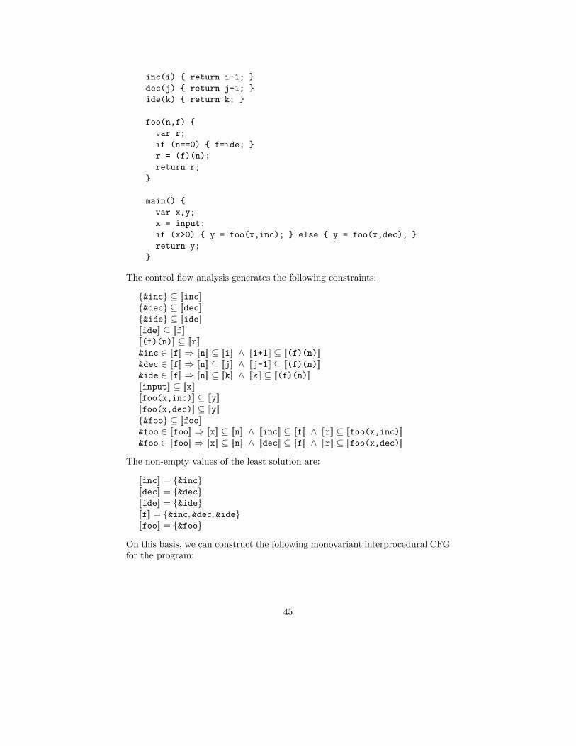
inc(i) { return i+1; }
dec(j) { return j-1; }
ide(k) { return k; }
foo(n,f) {
var r;
if (n==0) { f=ide; }
r = (f)(n);
return r;
}
main() {
var x,y;
x = input;
if (x>0) { y = foo(x,inc); } else { y = foo(x,dec); }
return y;
}
The control flow analysis generates the following constraints:
{&inc} ⊆ [[inc]]{&dec} ⊆ [[dec]]{&ide} ⊆ [[ide]][[ide]] ⊆ [[f]][[(f)(n)]] ⊆ [[r]]&inc ∈ [[f]] ⇒ [[n]] ⊆ [[i]] ∧ [[i+1]] ⊆ [[(f)(n)]]&dec ∈ [[f]] ⇒ [[n]] ⊆ [[j]] ∧ [[j-1]] ⊆ [[(f)(n)]]&ide ∈ [[f]] ⇒ [[n]] ⊆ [[k]] ∧ [[k]] ⊆ [[(f)(n)]][[input]] ⊆ [[x]][[foo(x,inc)]] ⊆ [[y]][[foo(x,dec)]] ⊆ [[y]]{&foo} ⊆ [[foo]]&foo ∈ [[foo]] ⇒ [[x]] ⊆ [[n]] ∧ [[inc]] ⊆ [[f]] ∧ [[r]] ⊆ [[foo(x,inc)]]&foo ∈ [[foo]] ⇒ [[x]] ⊆ [[n]] ∧ [[dec]] ⊆ [[f]] ∧ [[r]] ⊆ [[foo(x,dec)]]
The non-empty values of the least solution are:
[[inc]] = {&inc}[[dec]] = {&dec}[[ide]] = {&ide}[[f]] = {&inc, &dec, &ide}[[foo]] = {&foo}
On this basis, we can construct the following monovariant interprocedural CFGfor the program:
45

var x,y
x = input
x > 0
save−1−x=x save−2−x=x
save−1−y=y save−2−y=y
n = x n = x
f = inc f = dec
x=save−1−x x=save−2−x
y=save−1−y y=save−2−y
y = call−1 y = call−2
ret−main=y
call−1=ret−foo
call−2=ret−foo
var r
n==0
f = ide
save−3−r=r
r=save−3−r
r = call−3
ret−foo=r
ret−inc=i+1 ret−dec=j−1 ret−ide=k
call−3=ret−inc call−3=ret−dec call−3=ret−ide
which then can be used as basis for subsequent interprocedural static analyses.
Class Hierarchy Analysis
A language with function pointers or higher-order functions must use this kindof control flow analysis to obtain a reasonably precise CFG. For object-orientedlanguage it is also useful, but the added structure provided by the class hierarchyand the type system permits some simpler alternatives. In the object-orientedsetting the question is which method implementations may be executed at agiven method invocation site:
x.m(a,b,c)
The simplest solution is to scan the class library and select any method namedm whose signature accepts the types of the actual arguments. A better choice,called Class Hierarchy Analysis (CHA), is to consider only the part of the classhierarchy that is spanned by the declared type of x. A further refinement,called Rapid Type Analysis (RTA), is to restrict further to the classes of whichobjects are actually allocated. A final technique, called Variable Type Analysis
46
(VTA), performs intraprocedural control flow analysis while making conservativeassumptions about the remaining program.
These techniques are of course much faster than full-blown control flow anal-ysis, and for real-life programs they are also sufficiently precise.
11 Pointer Analysis
The final extension of the TIP language introduces simple pointers and dynamicmemory. Since our toy version of malloc only allocates a single cell, we can-not build arbitrary structures in the heap. However, the main problems withpointers are amply represented in the language fragment that we consider.
Points-To Analysis
The most important information that must be obtained is the set of possibletargets of pointers. There are of course infinitely many possible targets duringexecution, so we must select some finite representatives. The canonical choiceis to introduce a target &id for every variable named id and a target malloc-i,where i is a unique index, for each different allocation site (program point thatperforms a malloc operation). We use Targets to denote the set of pointertargets for a given program.
Points-to analysis takes place on the syntax tree, since it will happen beforeor simultaneously with the control flow analysis. The end result of a points-toanalysis is a function pt that for each (pointer) variable p returns the set pt(p)of possible pointer targets to which it may evaluate. We must of course performa conservative analysis, so these sets will in general be too large.
Given this information, many other facts can be approximated. If we wishto know whether pointer variables p and q may be aliases, then a safe answeris obtained by checking whether pt(p) ∩ pt(q) is non-empty.
The simplest analysis possible, called address taken, is to use all possibletargets, except that &id is only included if this construction occurs in the givenprogram. This only works for very simple applications, so more ambitious ap-proaches are usually preferred. If we restrict ourselves to typable programs,then any points-to analysis could be improved by removing those targets whosetypes are not equal to that of the pointer variable.
Andersen’s Algorithm
One approach to points-to analysis is quite similar to control flow analysis. Foreach variable named id we introduce a set variable [[id ]] ranging over the possiblepointer targets in the given program.
The analysis assumes that the program has been normalized so that everypointer manipulation is of one of the six kinds:
1) id = malloc
2) id1 = &id2
47
3) id1 = id2
4) id1 = *id2
5) *id1 = id2
6) id = null
Exercise 11.1: Show how this normalization can be performed systemati-cally by introducing fresh temporary variables.
For each of these pointer manipulations we then generate the following con-straints:
id = malloc: {malloc-i} ⊆ [[id ]]id1 = &id2: {&id2} ⊆ [[id1]]id1 = id2: [[id2]] ⊆ [[id1]]
id1 = *id2: &id ∈ [[id2]] ⇒ [[id ]] ⊆ [[id1]]*id1 = id2: &id ∈ [[id1]] ⇒ [[id2]] ⊆ [[id ]]
The last two constraints are generated for every variable named id, but weneed in fact only consider those whose addresses are actually taken in the givenprogram. The null assignment is ignored, since it corresponds to the constraint∅ ⊆ [[id ]]. Since these constraints match the requirements of the cubic algorithm,they can be solved in time O(n3). The resulting points-to function is definedas:
pt(p) = [[p]]
Consider the following example program:
var p,q,x,y,z;
p = malloc;
x = y;
x = z;
*p = z;
p = q;
q = &y;
x = *p;
p = &z;
Andersen’s algorithm generates these constraints:
malloc-1 ⊆ [[p]][[y]] ⊆ [[x]][[z]] ⊆ [[x]]&y ∈ [[p]] ⇒ [[z]] ⊆ [[y]]&z ∈ [[p]] ⇒ [[z]] ⊆ [[z]][[q]] ⊆ [[p]]{&y} ⊆ [[q]]&y ∈ [[p]] ⇒ [[y]] ⊆ [[x]]&z ∈ [[p]] ⇒ [[z]] ⊆ [[x]]{&z} ⊆ [[p]]
48
The non-empty values in the least solution are:
pt(p) = [[p]] = {malloc-1, &y, &z}pt(q) = [[q]] = {&y}
which gives a really precise result. Note that while this algorithm is flow in-sensitive, the directionality of the constraints implies that the dataflow is stillmodeled with some accuracy.
Steensgaard’s Algorithm
A popular alternative performs a coarser analysis essentially by viewing assign-ments as being bidirectional. This time we use a set consisting of the malloc-i
tokens and two tokens of the form id and *id for each variable named id. We usethe same normalized program as before, but this time we generate equivalenceconstraints on tokens:
id = malloc: *id ∼ malloc-i
id1 = &id2: *id1 ∼ id2
id1 = id2: id1 ∼ id2
id1 = *id2: id1 ∼ *id2
*id1 = id2: *id1 ∼ id2
The generated constraints induce an equivalence relation on the tokens, whichcan be computed in almost linear time. The resulting points-to function isdefined as:
pt(p) = {&id | *p ∼ id} ∪ {malloc-i | *p ∼ malloc-i}
Again, we might as well restrict ourselves to those instances of &id that occur inthe given program. If we only consider typable programs, then we can furthereliminate those targets whose types do not match.
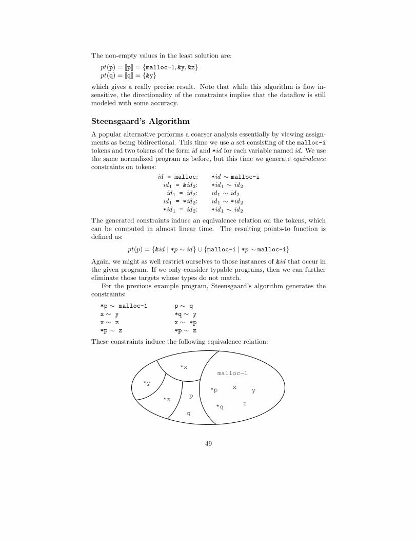
For the previous example program, Steensgaard’s algorithm generates theconstraints:
*p ∼ malloc-1 p ∼ q
x ∼ y *q ∼ y
x ∼ z x ∼ *p
*p ∼ z *p ∼ z
These constraints induce the following equivalence relation:
malloc−1
*p
*q
x y
zp
q
*x
*y
*z
49
This in turn implies that:
pt(p) = pt(q) = {malloc-1, &x, &y, &z}
which is significantly less precise than Andersen’s algorithm. Restricting to theaddresses that are actually taken, we obtain:
pt(p) = pt(q) = {malloc-1, &y, &z}
which for p is as precise as Andersen’s algorithm, but still is worse for q.
Interprocedural Points-To Analysis
If function pointers are distinguished from other pointers, then we can performan interprocedural points-to analysis by first computing an interprocedural CFGas described earlier and then running either Andersen’s or Steensgaard’s algo-rithm. If, however, function pointers may have indirect references as well thenwe need to perform the control flow analysis and the points-to analysis simul-taneously to resolve for example the function call:
(***x)(1,2,3);
To express the combined algorithm, we make the syntactic simplification thatall function calls are of the form:
id1 = (id2)(a1,. . . , an);
where id i and ai are variables. Similarly, all return expressions are assumed tobe just variables.
Exercise 11.2: Show how to perform these simplifications in a systematicmanner.
Andersen’s algorithm is already similar to control flow analysis, and it cansimply be extended with the appropriate constraints. A reference to a constantfunction f generates the constraint:
{&f } ⊆ [[f ]]
The computed function call generates the constraint:
&f ∈ [[id2]] ⇒ [[a1]] ⊆ [[x1]] ∧ . . . ∧ [[an]] ⊆ [[xn]] ∧ [[id ]] ⊆ [[id1]]
for every occurrence of a function definition:
f (x 1,. . . ,xn) { . . .return id; }
This will maintain the precision of the control flow analysis. In contrast, Steens-gaard’s algorithm would be extended with the constraint:
a1 ∼ x1 ∧ . . . ∧ an ∼ xn ∧ id ∼ id1
which results in a considerable loss of precision, since every n-argument functionis considered a possible target for the call.
50
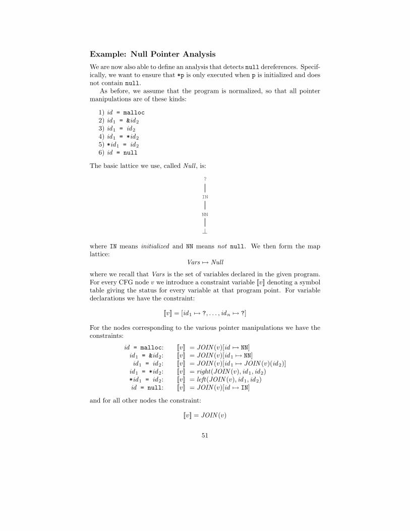
Example: Null Pointer Analysis
We are now also able to define an analysis that detects null dereferences. Specif-ically, we want to ensure that *p is only executed when p is initialized and doesnot contain null.
As before, we assume that the program is normalized, so that all pointermanipulations are of these kinds:
1) id = malloc
2) id1 = &id2
3) id1 = id2
4) id1 = *id2
5) *id1 = id2
6) id = null
The basic lattice we use, called Null , is:
NN
IN
?
where IN means initialized and NN means not null. We then form the maplattice:
Vars 7→ Null
where we recall that Vars is the set of variables declared in the given program.For every CFG node v we introduce a constraint variable [[v]] denoting a symboltable giving the status for every variable at that program point. For variabledeclarations we have the constraint:
[[v]] = [id1 7→ ?, . . . , idn 7→ ?]
For the nodes corresponding to the various pointer manipulations we have theconstraints:
id = malloc: [[v]] = JOIN (v)[id 7→ NN]id1 = &id2: [[v]] = JOIN (v)[id 1 7→ NN]id1 = id2: [[v]] = JOIN (v)[id 1 7→ JOIN (v)(id2)]
id1 = *id2: [[v]] = right(JOIN (v), id1, id2)*id1 = id2: [[v]] = left(JOIN (v), id1, id2)id = null: [[v]] = JOIN (v)[id 7→ IN]
and for all other nodes the constraint:
[[v]] = JOIN (v)
51
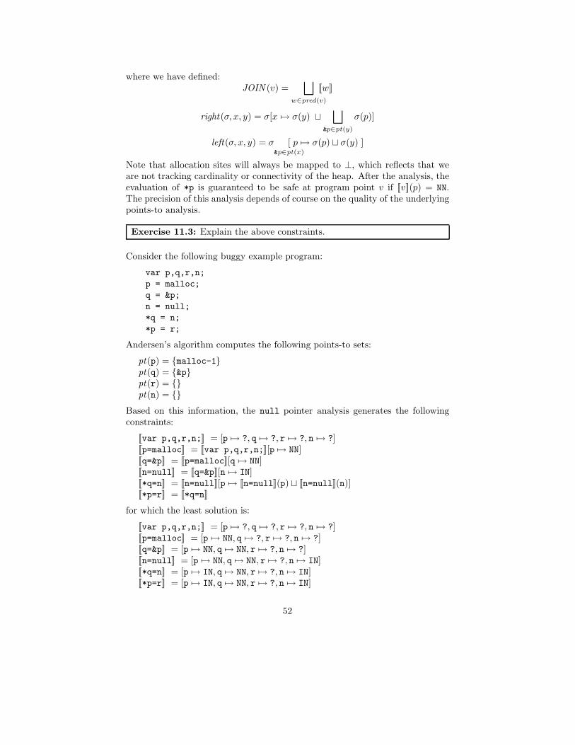
where we have defined:JOIN (v) =
⊔
w∈pred(v)
[[w]]
right(σ, x, y) = σ[x 7→ σ(y) ⊔⊔
&p∈pt(y)
σ(p)]
left(σ, x, y) = σ [&p∈pt(x)
p 7→ σ(p) ⊔ σ(y) ]
Note that allocation sites will always be mapped to ⊥, which reflects that weare not tracking cardinality or connectivity of the heap. After the analysis, theevaluation of *p is guaranteed to be safe at program point v if [[v]](p) = NN.The precision of this analysis depends of course on the quality of the underlyingpoints-to analysis.
Exercise 11.3: Explain the above constraints.
Consider the following buggy example program:
var p,q,r,n;
p = malloc;
q = &p;
n = null;
*q = n;
*p = r;
Andersen’s algorithm computes the following points-to sets:
pt(p) = {malloc-1}pt(q) = {&p}pt(r) = {}pt(n) = {}
Based on this information, the null pointer analysis generates the followingconstraints:
[[var p,q,r,n;]] = [p 7→ ?, q 7→ ?, r 7→ ?, n 7→ ?][[p=malloc]] = [[var p,q,r,n;]][p 7→ NN][[q=&p]] = [[p=malloc]][q 7→ NN][[n=null]] = [[q=&p]][n 7→ IN][[*q=n]] = [[n=null]][p 7→ [[n=null]](p) ⊔ [[n=null]](n)][[*p=r]] = [[*q=n]]
for which the least solution is:
[[var p,q,r,n;]] = [p 7→ ?, q 7→ ?, r 7→ ?, n 7→ ?][[p=malloc]] = [p 7→ NN, q 7→ ?, r 7→ ?, n 7→ ?][[q=&p]] = [p 7→ NN, q 7→ NN, r 7→ ?, n 7→ ?][[n=null]] = [p 7→ NN, q 7→ NN, r 7→ ?, n 7→ IN][[*q=n]] = [p 7→ IN, q 7→ NN, r 7→ ?, n 7→ IN][[*p=r]] = [p 7→ IN, q 7→ NN, r 7→ ?, n 7→ IN]
52
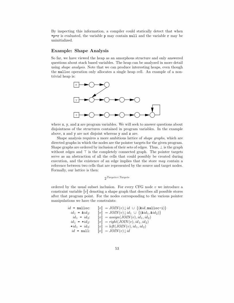
By inspecting this information, a compiler could statically detect that when*p=r is evaluated, the variable p may contain null and the variable r may beuninitialized.
Example: Shape Analysis
So far, we have viewed the heap as an amorphous structure and only answeredquestions about stack based variables. The heap can be analyzed in more detailusing shape analysis. Note that we can produce interesting heaps, even thoughthe malloc operation only allocates a single heap cell. An example of a non-trivial heap is:
x
y
z
where x, y, and z are program variables. We will seek to answer questions aboutdisjointness of the structures contained in program variables. In the exampleabove, x and y are not disjoint whereas y and z are.
Shape analysis requires a more ambitious lattice of shape graphs, which aredirected graphs in which the nodes are the pointer targets for the given program.Shape graphs are ordered by inclusion of their sets of edges. Thus, ⊥ is the graphwithout edges and ⊤ is the completely connected graph. The pointer targetsserve as an abstraction of all the cells that could possibly be created duringexecution, and the existence of an edge implies that the store may contain areference between two cells that are represented by the source and target nodes.Formally, our lattice is then:
2Targets×Targets
ordered by the usual subset inclusion. For every CFG node v we introduce aconstraint variable [[v]] denoting a shape graph that describes all possible storesafter that program point. For the nodes corresponding to the various pointermanipulations we have the constraints:
id = malloc: [[v]] = JOIN (v)↓ id ∪ {(&id , malloc-i)}id1 = &id2: [[v]] = JOIN (v)↓ id1 ∪ {(&id1, &id2)}id1 = id2: [[v]] = assign(JOIN (v), id1, id2)
id1 = *id2: [[v]] = right(JOIN (v), id1, id2)*id1 = id2: [[v]] = left(JOIN (v), id1, id2)id = null: [[v]] = JOIN (v)↓ id
53
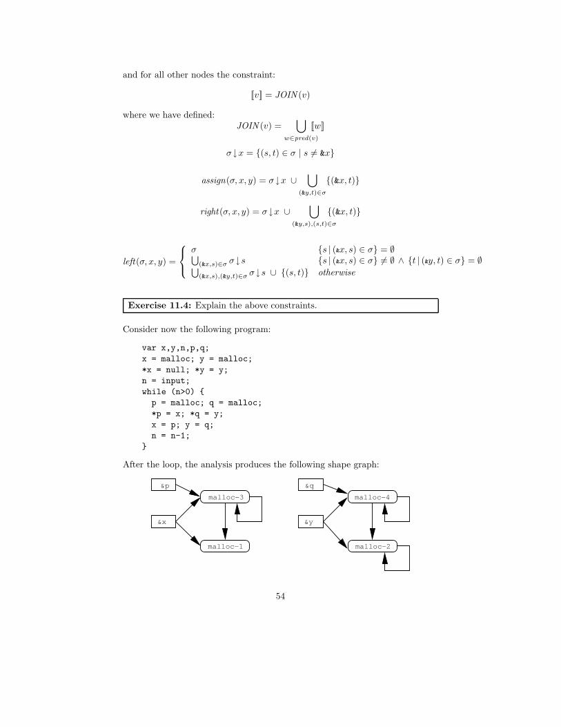
and for all other nodes the constraint:
[[v]] = JOIN (v)
where we have defined:JOIN (v) =
⋃
w∈pred(v)
[[w]]
σ↓x = {(s, t) ∈ σ | s 6= &x}
assign(σ, x, y) = σ↓x ∪⋃
(&y,t)∈σ
{(&x, t)}
right(σ, x, y) = σ↓x ∪⋃
(&y,s),(s,t)∈σ
{(&x, t)}
left(σ, x, y) =
σ {s | (&x, s) ∈ σ} = ∅⋃
(&x,s)∈σ σ↓s {s | (&x, s) ∈ σ} 6= ∅ ∧ {t | (&y, t) ∈ σ} = ∅⋃
(&x,s),(&y,t)∈σ σ↓s ∪ {(s, t)} otherwise
Exercise 11.4: Explain the above constraints.
Consider now the following program:
var x,y,n,p,q;
x = malloc; y = malloc;
*x = null; *y = y;
n = input;
while (n>0) {
p = malloc; q = malloc;
*p = x; *q = y;
x = p; y = q;
n = n-1;
}
After the loop, the analysis produces the following shape graph:
&x
malloc−3
malloc−1
malloc−4
malloc−2
&y
&p &q
54

From this result we can safely conclude that x and y will always be disjoint.Note that our shape analysis also computes a flow sensitive points-to map
that for each program point v is defined by:
pt(p) = {t | (&p, t) ∈ [[v]]}
This analysis is more precise than Andersen’s algorithm, but clearly also moreexpensive to perform. As an example, consider the program:
x = &y;
x = &z;
After these statements, Andersen’s algorithm would predict that pt(x) = {&y, &z}whereas the shape analysis computes pt(x) = {&z} for the final program point.This flow sensitive points-to information could be used to boost the null pointeranalysis. However, an initial flow insensitive points-to analysis would still berequired to construct a CFG for programs using function pointers. Conversely,if we have another points-to analysis, then it may be used to boost the precisionof the shape analysis by restricting the targets considered in the left and rightfunctions.
Example: Better Shape Analysis
The above shape analysis allows us to conclude that x and y will always bedisjoint. However, the shape graphs we compute are unable to answer otherinteresting questions. For example, we cannot conclude that malloc-2 nodesalways contain a self-loop whereas malloc-4 nodes never appear on cycles. Tomake such distinctions, we need a more detailed lattice. As an example, wecould maintain information about cyclicity in the graph. This would changeour lattice into:
2Targets×Targets × 2Targets×Targets
where for an element (X,Y ) we have that X denotes the possible edges andY ⊆ X denotes those edges that could possibly be part of a cycle in the graph(thus, Y is used to remember part of the history of the heap).
With this more detailed lattice we now get the obligation of correspondinglyupdating the constraints. Of course, we could trivially always consider thesecond component to contain all edges, but to obtain useful results we needto do better. An assignment id = malloc can never create a cycle, so thecorresponding constraint may be updated as follows (where we assume thatJOIN (v) = (X,Y )):
id = malloc: [[v]] = (X ↓ id ∪ {(&id , malloc-i)}, Y ↓ id)
An assignment id1 = &id2 cannot create a cycle if the current shape graph doesnot contain a path from &id2 to &id1 (since reachability in the shape graph isconservative). Consequently, the constraint may be updated as follows:
55
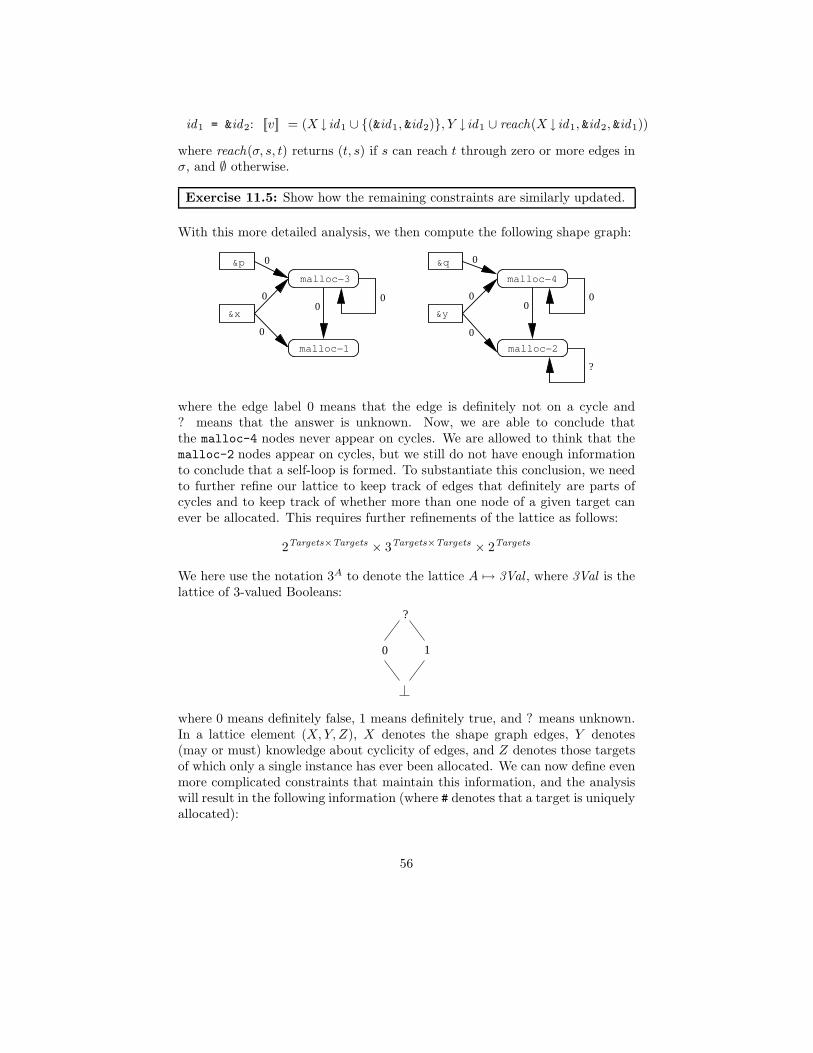
id1 = &id2: [[v]] = (X ↓ id1 ∪ {(&id1, &id2)}, Y ↓ id1 ∪ reach(X ↓ id1, &id2, &id1))
where reach(σ, s, t) returns (t, s) if s can reach t through zero or more edges inσ, and ∅ otherwise.
Exercise 11.5: Show how the remaining constraints are similarly updated.
With this more detailed analysis, we then compute the following shape graph:
&x
malloc−3
malloc−1
malloc−4
malloc−2
&y
&p &q
0
?
0
0
0
00
0
0
0
0
where the edge label 0 means that the edge is definitely not on a cycle and? means that the answer is unknown. Now, we are able to conclude thatthe malloc-4 nodes never appear on cycles. We are allowed to think that themalloc-2 nodes appear on cycles, but we still do not have enough informationto conclude that a self-loop is formed. To substantiate this conclusion, we needto further refine our lattice to keep track of edges that definitely are parts ofcycles and to keep track of whether more than one node of a given target canever be allocated. This requires further refinements of the lattice as follows:
2Targets×Targets × 3Targets×Targets × 2Targets
We here use the notation 3A to denote the lattice A 7→ 3Val , where 3Val is thelattice of 3-valued Booleans:
0
?
1
where 0 means definitely false, 1 means definitely true, and ? means unknown.In a lattice element (X,Y, Z), X denotes the shape graph edges, Y denotes(may or must) knowledge about cyclicity of edges, and Z denotes those targetsof which only a single instance has ever been allocated. We can now define evenmore complicated constraints that maintain this information, and the analysiswill result in the following information (where # denotes that a target is uniquelyallocated):
56

&x
malloc−3
malloc−1
malloc−4
malloc−2
&y
&p &q
0
1
0
0
0
00
0
0
0
0#
# #
#
# #
Finally, we are able to conclude that there is only a single malloc-2 node andthat it has a self-loop.
Analyses like the above can be performed in a less ad-hoc manner, using aframework known as parametric shape analysis. Here, the targets are character-ized by a number of unary instrumentation predicates that are chosen to providethe information necessary for the analysis. Examples of such unary predicatesare:
• does this node have two or more incoming pointers?
• is this node reachable from the variable x?
• is this node on a cycle?
but the relevant ones depend on the questions for which we seek answers. Oursimple shape graphs had a single node for each pointer target. In the parametricframework, we polyvariantly have a copy for each possible 3-valued interpreta-tion of the predicates. Thus, the nodes of a shape graph corresponds to:
3Targets × 3Targets × . . .× 3Targets
with one copy for each predicate. The shape graph itself must then describe theconnectivity between these nodes, and again we use 3-valued logic to describeedges as definitely present, definitely absent, or possibly present. Thus, our finallattice becomes:
3(3Targets×3Targets×...×3Targets)2
or (amusingly):
3((3Targets)k)2
if we have k predicates. To complete the parametric shape analysis, we mustthe specify the constraints. If we have included many predicates, then we have acorrespondingly heavy burden of maintaining these with useful precision. Thisis generally something of a puzzle to get right, as indicated even by our simpleexample above. But the technique is powerful and may be used to verify e.g.that a procedure for inserting into a red-black search tree respects the red-blackinvariant.
57
Example: Escape Analysis
We earlier lamented the escaping stack cell error displayed by the program:
baz() {
var x;
return &x;
}
main() {
var p;
p=baz(); *p=1;
return *p;
}
which was beyond the scope of the type system. Having performed the simpleshape analysis, we can easily perform an escape analysis to catch such errors.We just need to check that the possible pointer targets for return expressionsin the shape graph cannot reach arguments or variables defined in the functionitself, since all other pointer targets must then necessarily reside in earlier frameson the invocation stack.
12 Conclusion
We have seen the basic tools that are required to perform static analysis ofprograms. Real-life applications invariably gravitate back to the techniques thatwe have covered, though many variations and extensions are usually required.
Two major areas have not been covered at all. The quality of an analysiscan only be measured relatively to a suite of intended applications. It is rarethat competing analyses can be formally compared, so much work in this area isconcerned with performing experiments to establish the precision and efficiencyof proposed analyses. The correctness of an analysis requires a formal semanticsof the underlying programming language. Completely formal proofs of correct-ness of analyses are exceedingly laborious and remain mostly academic exercises.Even so, it is often possible to provide convincing correctness arguments.
Acknowledgement
Thanks to Aske Simon Christensen and Anders Møller for comments and ideas.
58