lecture place based policies - gspp.berkeley.edu

1

LECTURE: PLACE BASED POLICIES HILARY HOYNES UC DAVIS EC230 Jeffrey R. Kling, Jeffrey B. Liebman and Lawrence F. Katz,. Experimental Analysis of Neighborhood Effects, Econometrica, 75:1 (January 2007), 83-119 Pat Kline, Matias Busso, and Jesse Gregory, “Assessing the Incidence and Efficiency of a Prominent Place Based Policy”, working paper.

2

Kling et al, Econometrica, 2007 Paper is the culmination of several papers analyzing the Moving to

Opportunity Program (MTO) Super interesting research because it speaks to literature on:

o Neighborhood effects o Impacts of public housing

Limits to interpretation o What role does the impact of “moving” play? [moving is bundled with

moving to a better place] Influential set of papers because of the (a) clean experiment (relative to the

existing literature on neighborhood effects and impacts of public housing) and (b) wide set of outcomes analyzed, (c) exploring differential impacts by gender

3

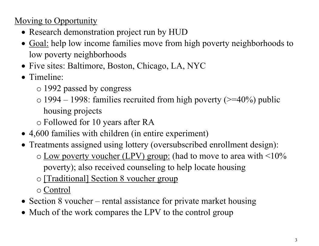
Moving to Opportunity Research demonstration project run by HUD Goal: help low income families move from high poverty neighborhoods to

low poverty neighborhoods Five sites: Baltimore, Boston, Chicago, LA, NYC Timeline:

o 1992 passed by congress o 1994 – 1998: families recruited from high poverty (>=40%) public

housing projects o Followed for 10 years after RA

4,600 families with children (in entire experiment) Treatments assigned using lottery (oversubscribed enrollment design):

o Low poverty voucher (LPV) group: (had to move to area with <10% poverty); also received counseling to help locate housing

o [Traditional] Section 8 voucher group o Control

Section 8 voucher – rental assistance for private market housing Much of the work compares the LPV to the control group

5

Some background before getting to Econometrica paper: Interim report (5-7 years after RA) Outcomes come from:

o Administrative data: earnings, AFDC/TANF, Food stamps, criminal justice system

o Surveys: household heads, youth ages 12-19, children 5-11

5

MTO Interim: Improved Neighborhood Outcomes (ITT)

All differences in outcome levels between the LPV group and the control group are statistically significant at the p<0.05 level.

0.46

0.21

0.15

0.87

0.24

0.45

0.33

0.52

0.17

0.34

0

0.1

0.2

0.3

0.4

0.5

0.6

0.7

0.8

0.9

1

Census Tract

Poverty Rate

Census Tract

Poverty >30%

Saw illicit

drugs sold or

used

Victim of crime Feels unsafe

during the day

Control Mean LPV Mean

6

MTO Interim: No effect on adult labor market outcomes but improved mental and physical health (ITT)

0.55

0.05

0.33

0.47

-0.04

0.53

0.350.42

-0.2

-0.1

0.0

0.1

0.2

0.3

0.4

0.5

0.6

0.7

0.8

0.9

Not working or on

TANF

Psychological

distress, K6 (z-

score) *

Has fair or poor

health

Obese, Body

Mass Index ≥ 30 *


* Difference in outcome levels between the LPV group and the control group is statistically significant at the p<0.05 level.

7

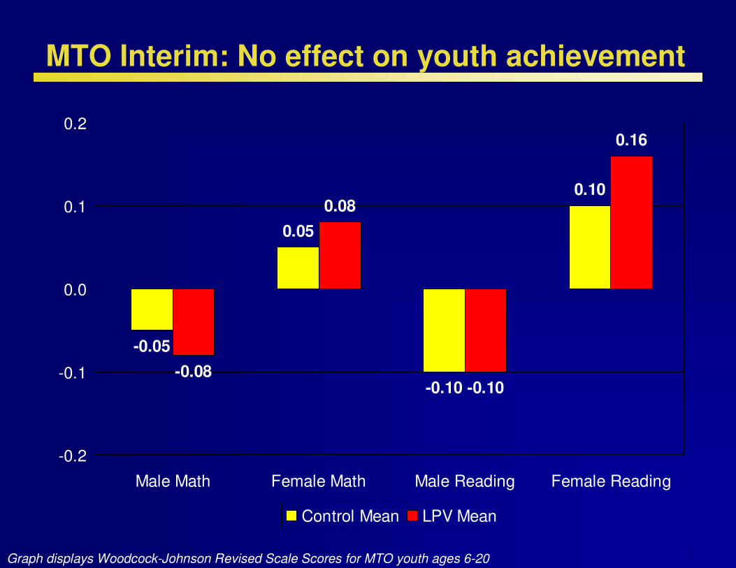
MTO Interim: No effect on youth achievement

-0.05

0.05

-0.10

0.10

-0.08

0.08

-0.10

0.16

-0.2

-0.1

0.0

0.1

0.2

Male Math Female Math Male Reading Female Reading


Graph displays Woodcock-Johnson Revised Scale Scores for MTO youth ages 6-20

8

MTO Interim: Less psychological distress & fewer behavior problems for female teens (ITT)

0.270.24

0.16

-0.02

0.23

0.110.13

0.07

-0.1

0.0

0.1

0.2

0.3

0.4

0.5

0.6

0.7

0.8

0.9

Psychological

distress K6, z-score

[ages 15-20] *

Used marijuana last

30 days [ages 15-

20]*

Behavior problems

index [ages 11-20]

# lifetime property

crime arrests [ages

15-25] *



9

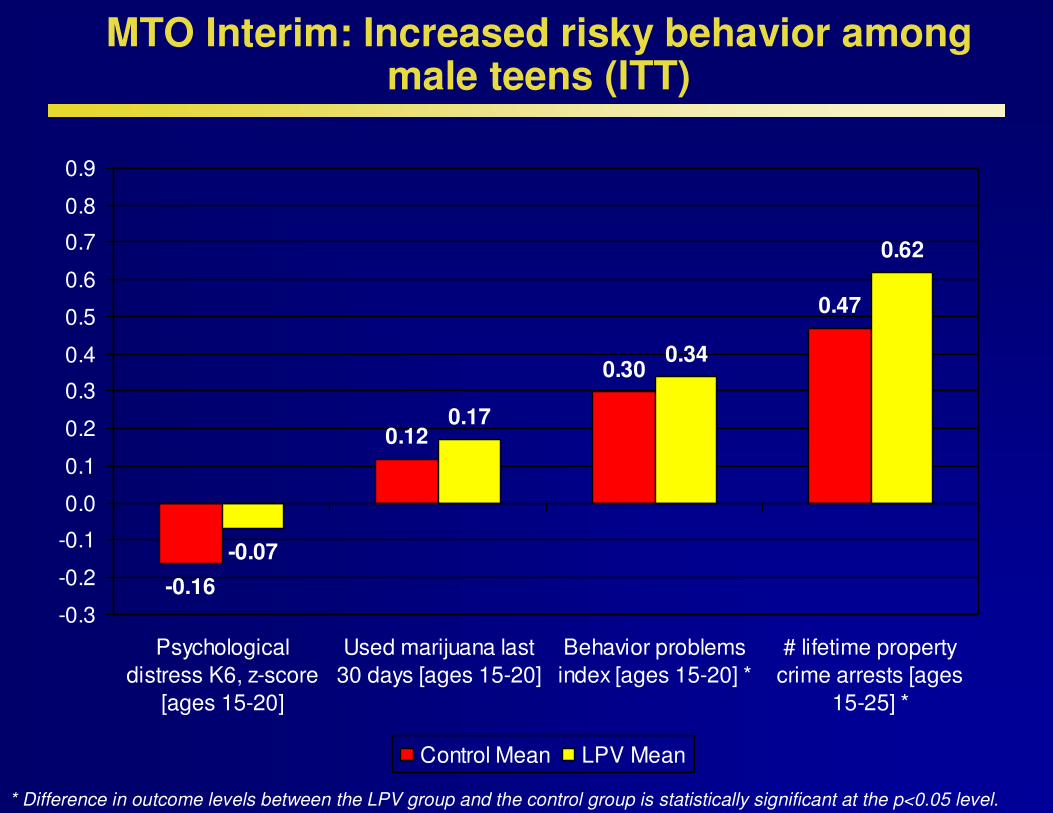
MTO Interim: Increased risky behavior among male teens (ITT)

-0.16

0.30

0.47

0.170.12

0.62

0.34

-0.07

-0.3

-0.2

-0.1

0.0

0.1

0.2

0.3

0.4

0.5

0.6

0.7

0.8

0.9

Psychological

distress K6, z-score

[ages 15-20]

Used marijuana last

30 days [ages 15-20]

Behavior problems

index [ages 15-20] *

# lifetime property

crime arrests [ages

15-25] *



7

So what does the Econometrica paper do that we don’t have in these results? Introduces the idea of “indices” for combining outcome variables Develops the idea of inference with multiple outcome variables (when there

might be correlation across them)

8

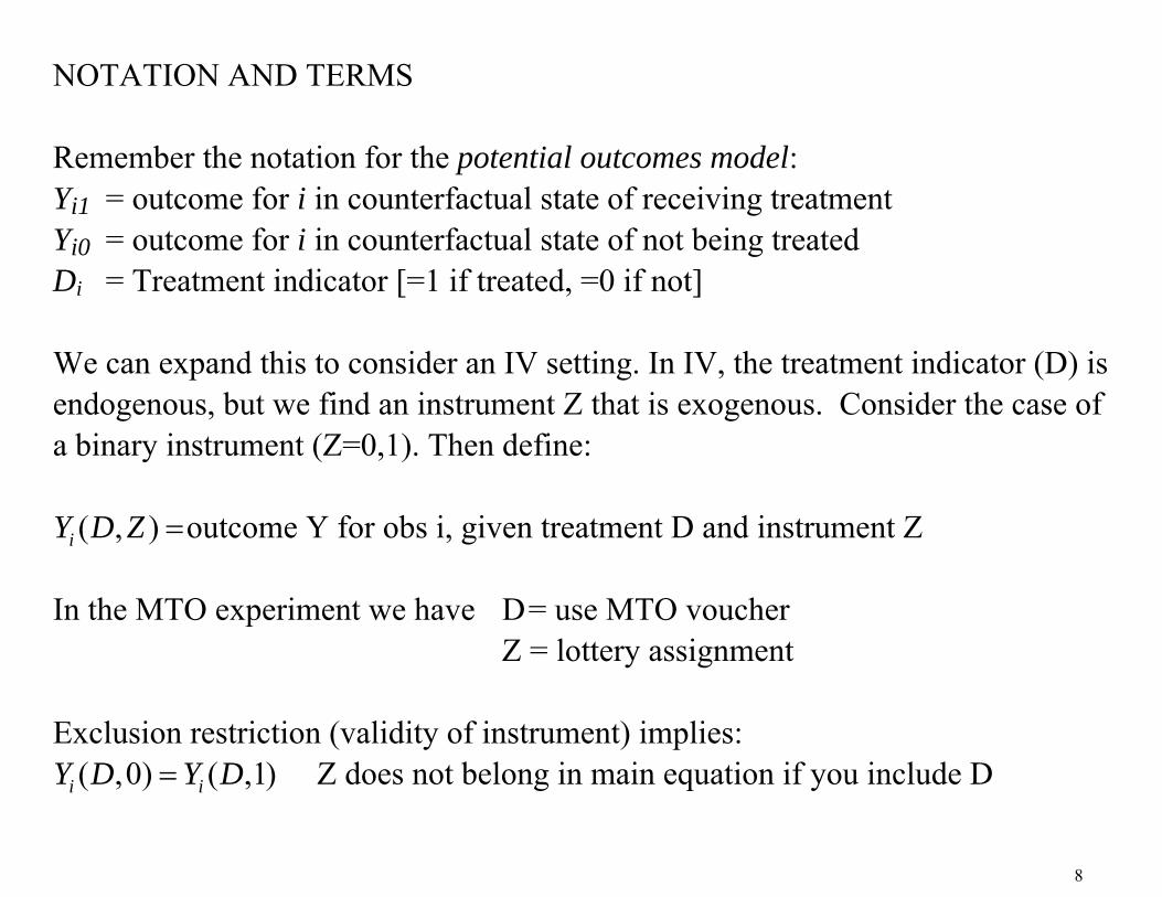
NOTATION AND TERMS Remember the notation for the potential outcomes model: Yi1 = outcome for i in counterfactual state of receiving treatment Yi0 = outcome for i in counterfactual state of not being treated Di = Treatment indicator [=1 if treated, =0 if not] We can expand this to consider an IV setting. In IV, the treatment indicator (D) is endogenous, but we find an instrument Z that is exogenous. Consider the case of a binary instrument (Z=0,1). Then define:

( , )iY D Z outcome Y for obs i, given treatment D and instrument Z In the MTO experiment we have D = use MTO voucher Z = lottery assignment Exclusion restriction (validity of instrument) implies:

( ,0) ( ,1)i iY D Y D Z does not belong in main equation if you include D

9

So, with that, we can use introduce the terms used in the paper: Compliers: The subpopulation with 1 1iD and 0 0iD .

In our example: those for whom assignment to the LPV moves them to a low poverty neighborhood. (or getting section 8 moves them into private housing)

Always-takers: The subpopulation with 1 0 1i iD D . Never-takers: The subpopulation with 1 0 0i iD D . Where 1iD i’s treatment status when assigned to Z = 1 0iD i’s treatment status when assigned to Z = 0 In this experiment, no one who is assigned to the control can end up with the “treatment” (= MTO voucher). In some experiments, you can still get access to D even if you do not get the lottery.

10

So if you regress: Y D Biased, since there is selection into D (even if you have an experiment) Y Z Intent to Treat; impacts on those who were offered treatment (these are the graphs we just looked at; simple T vs C comparisons) Causal IV: instrument D with Z Effect of treatment on the treated; divides the ITT by the difference in compliance rates (δ) between the treatment and control [reduced form divided by first stage as in Wald estimator]: D Z

11

Kling, Liebman and Katz, Econometrica, 2007 Data used is through the interim report (as we just saw); 5-7 years after RA Outcomes measured in five domains:

o Economic self sufficiency o Mental health o Physical health o Risky behavior o Education

Their analysis here covers adults and youth 15-20 Internal validity: they do not show any evidence on balance in lottery

assignment. They should External validity: very disadvantaged groups; 66% black, 62% never married,

38% high school grad (or more). The impact of the experiment is for those who volunteered to get this ticket out of the neighborhood.

What they call the three groups: Experimental = LPV treatment, Section 8 group, Control

12

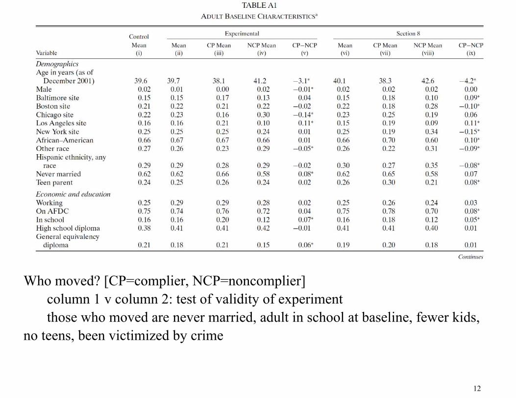
Who moved? [CP=complier, NCP=noncomplier] column 1 v column 2: test of validity of experiment those who moved are never married, adult in school at baseline, fewer kids, no teens, been victimized by crime

13

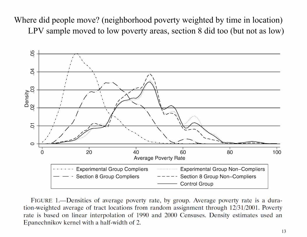
Where did people move? (neighborhood poverty weighted by time in location) LPV sample moved to low poverty areas, section 8 did too (but not as low)

14

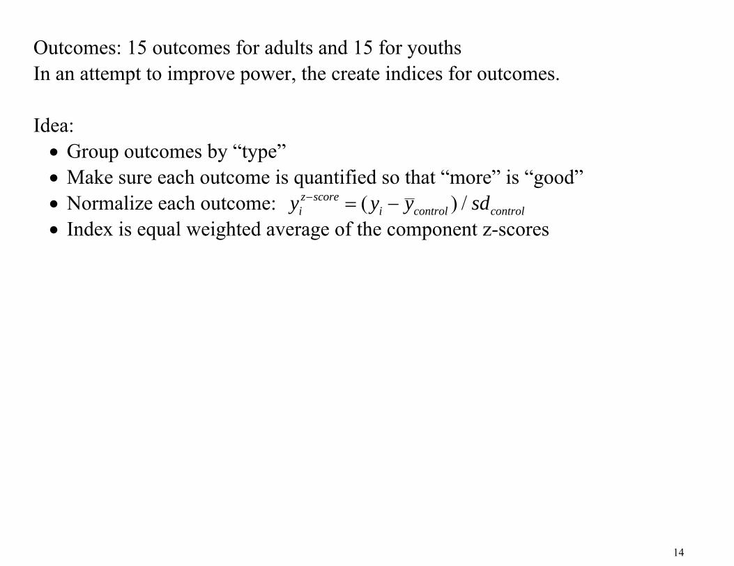
Outcomes: 15 outcomes for adults and 15 for youths In an attempt to improve power, the create indices for outcomes. Idea: Group outcomes by “type” Make sure each outcome is quantified so that “more” is “good” Normalize each outcome: ( ) /z score

i i control controly y y sd Index is equal weighted average of the component z-scores

15

ITT results, 1 1 1Y Z X (add Xs to improve precision)

Results are in SD units Focusing on the results for E treatment, Adults: better mental health Girls: across the board better Boys: across the board worse [qualitatively similar to graphs earlier]

16

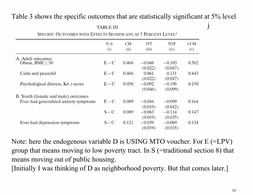
Table 3 shows the specific outcomes that are statistically significant at 5% level j

Note: here the endogenous variable D is USING MTO voucher. For E (=LPV) group that means moving to low poverty tract. In S (=traditional section 8) that means moving out of public housing. [Initially I was thinking of D as neighborhood poverty. But that comes later.]

17

How to learn about impacts of neighborhood:

3 3 3Y W X

W = neighborhood poverty They (a) pool both treatment groups (I am not sure why)

(b) instrument with site (5) x treatment (2) dummies (I am not sure why they now introduce site location here)

This seems like a weird set up. (I think they do this because they in turn estimate a model with W and D in it. They want to identify the effect of moving from the change in poverty. There they need 2 instruments—two endog vars—so they bring them in here.) But, if X only includes site FE then using wald estimator type intuition, that tells us that γ will be identified by the reduced form scaled by the first stage (effect of assignment on poverty rate) We can then look at the results visually:

18

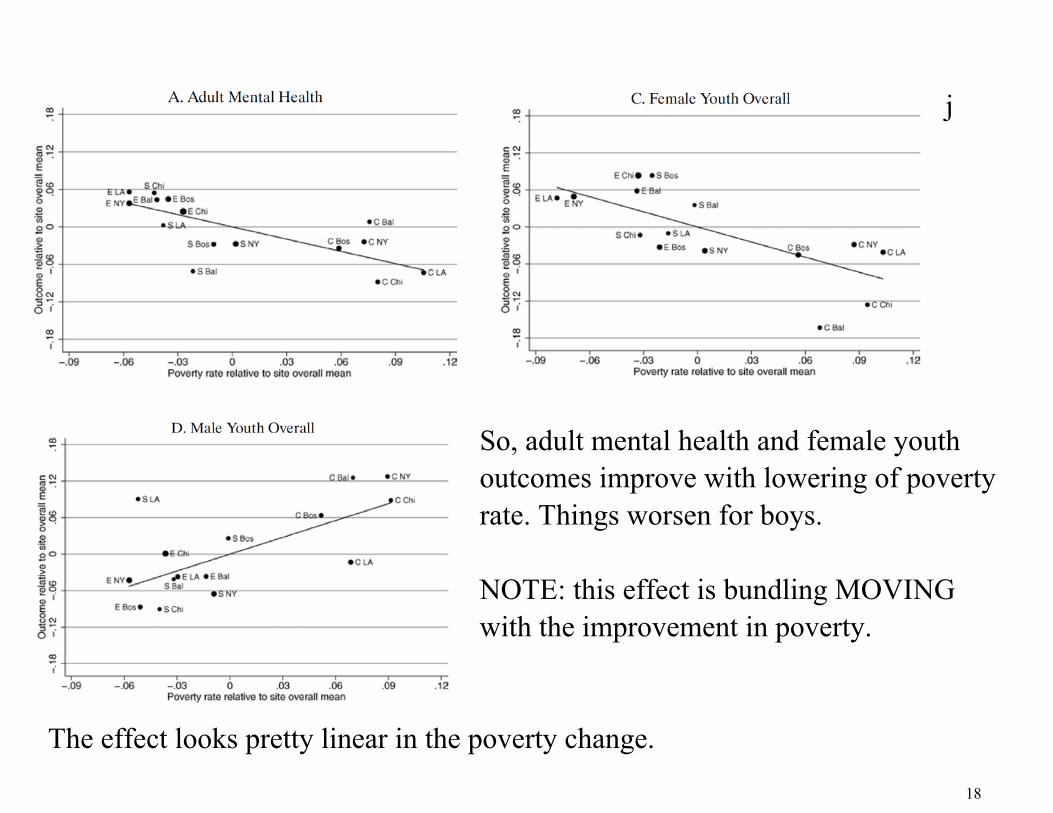
j

So, adult mental health and female youth outcomes improve with lowering of poverty rate. Things worsen for boys. NOTE: this effect is bundling MOVING with the improvement in poverty.

The effect looks pretty linear in the poverty change.

19

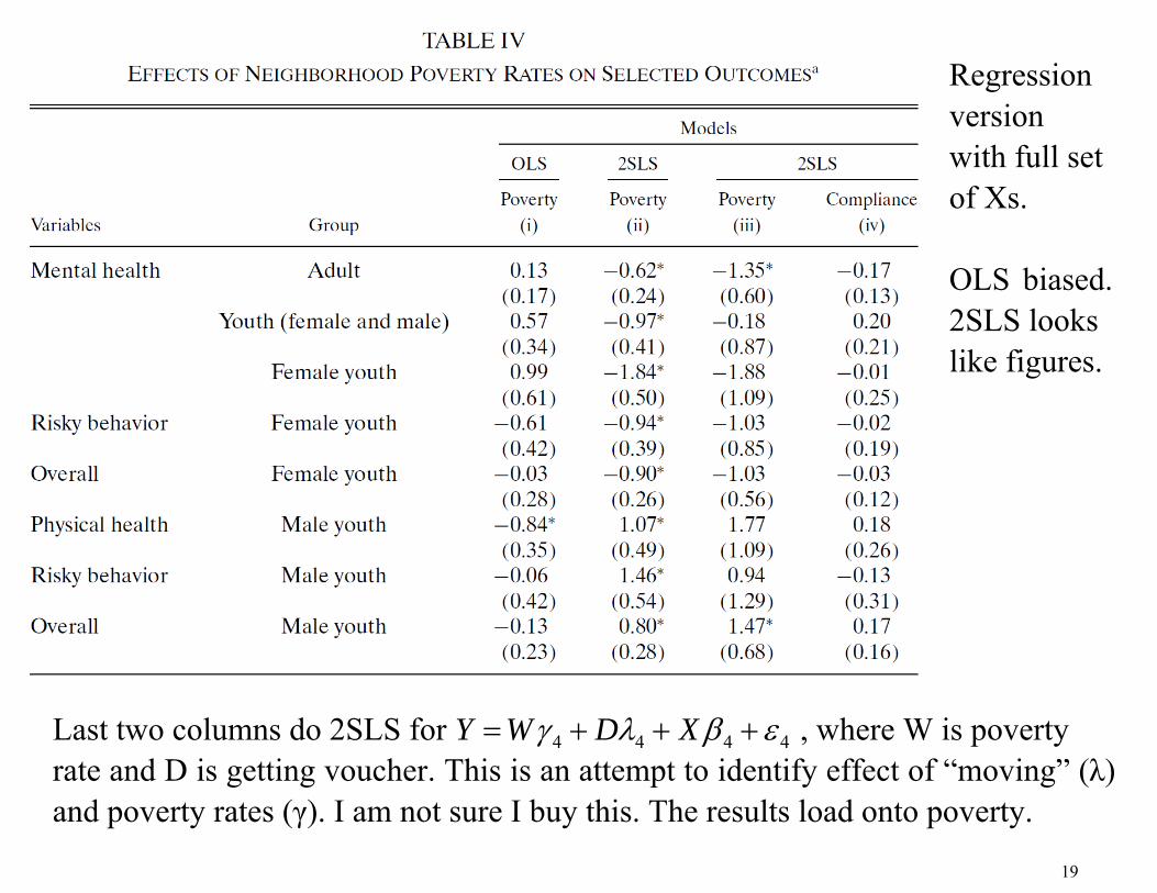
Regression version with full set of Xs. OLS biased. 2SLS looks like figures.

Last two columns do 2SLS for 4 4 4 4Y W D X , where W is poverty rate and D is getting voucher. This is an attempt to identify effect of “moving” (λ) and poverty rates (γ). I am not sure I buy this. The results load onto poverty.

20

Multiple outcome inference Basic idea is that if we look at lots of outcomes, one is likely to be significant even if under the null there is no effect. Further, one would expect correlation in the errors across the different outcome equations. This paper is often referenced for its accounting for this “multiple outcome” inference. I was surprised to see that this is not really laid out in the paper. Footnote 27: “The probability that the second largest t-statistic among 30 adult estimates is 2.2 or higher under the joint null hypothesis of no effect is a familywise adjusted p-value of 0.80, which is indicative of the fact that there is little power to reject the joint null hypothesis for specific outcomes. The adjusted p-values throughout this paper are based on a bootstrap procedure that accounts for covariance among estimates, using a method adapted fromWestfall and Young (1993) as described in Appendix B of the Web Appendix.”

21

Other thoughts and observations: On p. 104 they reveal that there was imbalance in the boys at baseline (LPV

group with worse outcomes). Yikes mention it this late! Their hypotheses for why boys do worse: less contact with male role models,

cultural isolation

lecture place based policies - gspp.berkeley.edu

Documents