lecture slides on nonlinear programming … · lecture slides on nonlinear programming based on...

LECTURE SLIDES ON NONLINEAR PROGRAMMING

BASED ON LECTURES GIVEN AT THE

MASSACHUSETTS INSTITUTE OF TECHNOLOGY

CAMBRIDGE, MASS

DIMITRI P. BERTSEKAS

These lecture slides are based on the book:“Nonlinear Programming,” Athena Scientific,by Dimitri P. Bertsekas; see

http://www.athenasc.com/nonlinbook.html

for errata, selected problem solutions, and othersupport material.

The slides are copyrighted but may be freelyreproduced and distributed for any noncom-mercial purpose.

LAST REVISED: Feb. 3, 2005

6.252 NONLINEAR PROGRAMMING

LECTURE 1: INTRODUCTION

LECTURE OUTLINE

• Nonlinear Programming

• Application Contexts

• Characterization Issue

• Computation Issue

• Duality

• Organization

NONLINEAR PROGRAMMING

minx∈X

f(x),

where

• f : �n �→ � is a continuous (and usually differ-entiable) function of n variables

• X = �n or X is a subset of �n with a “continu-ous” character.

• If X = �n, the problem is called unconstrained

• If f is linear and X is polyhedral, the problemis a linear programming problem. Otherwise it isa nonlinear programming problem

• Linear and nonlinear programming have tradi-tionally been treated separately. Their method-ologies have gradually come closer.

TWO MAIN ISSUES

• Characterization of minima

− Necessary conditions

− Sufficient conditions

− Lagrange multiplier theory

− Sensitivity

− Duality

• Computation by iterative algorithms

− Iterative descent

− Approximation methods

− Dual and primal-dual methods

APPLICATIONS OF NONLINEAR PROGRAMMING

• Data networks – Routing

• Production planning

• Resource allocation

• Computer-aided design

• Solution of equilibrium models

• Data analysis and least squares formulations

• Modeling human or organizational behavior

CHARACTERIZATION PROBLEM

• Unconstrained problems

− Zero 1st order variation along all directions

• Constrained problems

− Nonnegative 1st order variation along all fea-sible directions

• Equality constraints

− Zero 1st order variation along all directionson the constraint surface

− Lagrange multiplier theory

• Sensitivity

COMPUTATION PROBLEM

• Iterative descent

• Approximation

• Role of convergence analysis

• Role of rate of convergence analysis

• Using an existing package to solve a nonlinearprogramming problem

POST-OPTIMAL ANALYSIS

• Sensitivity

• Role of Lagrange multipliers as prices

DUALITY

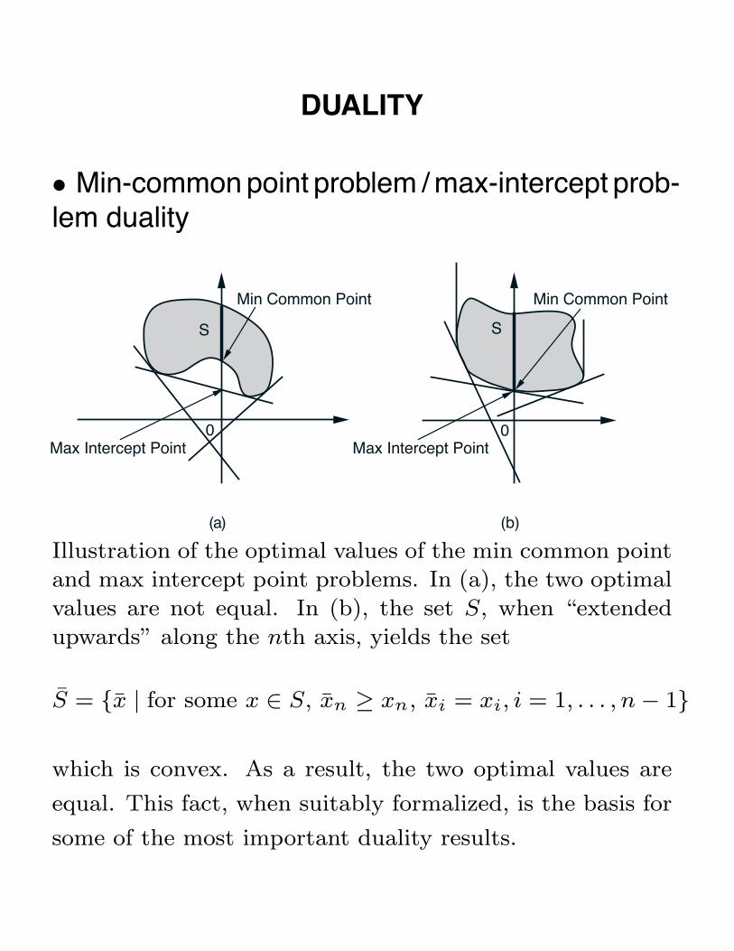
• Min-common point problem / max-intercept prob-lem duality

0 0

(a) (b)

Min Common Point

Max Intercept Point Max Intercept Point

Min Common Point

S S

Illustration of the optimal values of the min common point

and max intercept point problems. In (a), the two optimal

values are not equal. In (b), the set S, when “extended

upwards” along the nth axis, yields the set

S̄ = {x̄ | for some x ∈ S, x̄n ≥ xn, x̄i = xi, i = 1, . . . , n − 1}

which is convex. As a result, the two optimal values are

equal. This fact, when suitably formalized, is the basis for

some of the most important duality results.


LECTURE 2

UNCONSTRAINED OPTIMIZATION -

OPTIMALITY CONDITIONS

LECTURE OUTLINE

• Unconstrained Optimization

• Local Minima

• Necessary Conditions for Local Minima

• Sufficient Conditions for Local Minima

• The Role of Convexity

MATHEMATICAL BACKGROUND

• Vectors and matrices in �n

• Transpose, inner product, norm

• Eigenvalues of symmetric matrices

• Positive definite and semidefinite matrices

• Convergent sequences and subsequences

• Open, closed, and compact sets

• Continuity of functions

• 1st and 2nd order differentiability of functions

• Taylor series expansions

• Mean value theorems

LOCAL AND GLOBAL MINIMA

f(x)

x

Strict LocalMinimum

Local Minima Strict GlobalMinimum

Unconstrained local and global minima in one dimension.

NECESSARY CONDITIONS FOR A LOCAL MIN

• 1st order condition: Zero slope at a localminimum x∗

∇f(x∗) = 0

• 2nd order condition: Nonnegative curvatureat a local minimum x∗

∇2f(x∗) : Positive Semidefinite

• There may exist points that satisfy the 1st and2nd order conditions but are not local minima

x xx

f(x) = |x|3 (convex) f(x) = x3 f(x) = - |x|3

x* = 0 x* = 0x* = 0

First and second order necessary optimality conditions for

functions of one variable.

PROOFS OF NECESSARY CONDITIONS

• 1st order condition ∇f(x∗) = 0. Fix d ∈ �n.Then (since x∗ is a local min), from 1st order Taylor

d′∇f(x∗) = limα↓0

f(x∗ + αd) − f(x∗)α

≥ 0,

Replace d with −d, to obtain

d′∇f(x∗) = 0, ∀ d ∈ �n

• 2nd order condition ∇2f(x∗) ≥ 0. From 2ndorder Taylor

f(x∗+αd)−f(x∗) = α∇f(x∗)′d+α2

2d′∇2f(x∗)d+o(α2)

Since ∇f(x∗) = 0 and x∗ is local min, there issufficiently small ε > 0 such that for all α ∈ (0, ε),

0 ≤ f(x∗ + αd) − f(x∗)α2

= 12d

′∇2f(x∗)d +o(α2)α2

Take the limit as α → 0.

SUFFICIENT CONDITIONS FOR A LOCAL MIN

• 1st order condition: Zero slope

∇f(x∗) = 0

• 1st order condition: Positive curvature

∇2f(x∗) : Positive Definite

• Proof: Let λ > 0 be the smallest eigenvalue of∇2f(x∗). Using a second order Taylor expansion,we have for all d

f(x∗ + d) − f(x∗) = ∇f(x∗)′d +12d′∇2f(x∗)d

+ o(‖d‖2)

≥ λ

2‖d‖2 + o(‖d‖2)

=(

λ

2+

o(‖d‖2)‖d‖2

)‖d‖2.

For ‖d‖ small enough, o(‖d‖2)/‖d‖2 is negligiblerelative to λ/2.

CONVEXITY

Convex Sets Nonconvex Sets

x

y

αx + (1 - α)y, 0 < α < 1

x

x

y

y

xy

Convex and nonconvex sets.

αf(x) + (1 - α)f(y)

x y

C

z

f(z)

A convex function. Linear interpolation underestimates

the function.

MINIMA AND CONVEXITY

• Local minima are also global under convexity

αf(x*) + (1 - α)f(x)

x

f(αx* + (1- α)x)

x x*

f(x)

Illustration of why local minima of convex functions are

also global. Suppose that f is convex and that x∗ is a

local minimum of f . Let x be such that f(x) < f(x∗). By

convexity, for all α ∈ (0, 1),

f(αx∗ + (1 − α)x

)≤ αf(x∗) + (1 − α)f(x) < f(x∗).

Thus, f takes values strictly lower than f(x∗) on the line

segment connecting x∗ with x, and x∗ cannot be a local

minimum which is not global.

OTHER PROPERTIES OF CONVEX FUNCTIONS

• f is convex if and only if the linear approximationat a point x based on the gradient, underestimatesf :

f(z) ≥ f(x) + ∇f(x)′(z − x), ∀ z ∈ �n

f(z)f(z) + (z - x)'∇f(x)

x z

− Implication:

∇f(x∗) = 0 ⇒ x∗ is a global minimum

• f is convex if and only if ∇2f(x) is positivesemidefinite for all x


LECTURE 3: GRADIENT METHODS

LECTURE OUTLINE

• Quadratic Unconstrained Problems

• Existence of Optimal Solutions

• Iterative Computational Methods

• Gradient Methods - Motivation

• Principal Gradient Methods

• Gradient Methods - Choices of Direction

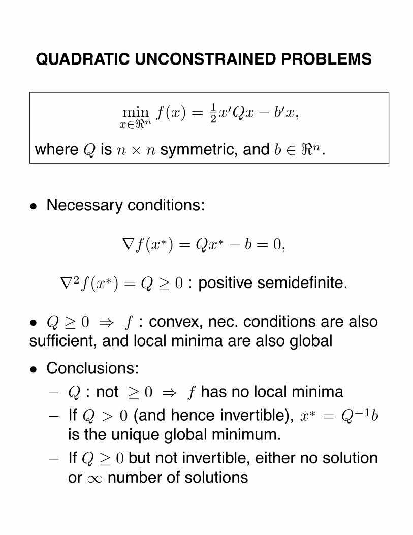
QUADRATIC UNCONSTRAINED PROBLEMS

minx∈�n

f(x) = 12x′Qx − b′x,

where Q is n × n symmetric, and b ∈ �n.

• Necessary conditions:

∇f(x∗) = Qx∗ − b = 0,

∇2f(x∗) = Q ≥ 0 : positive semidefinite.

• Q ≥ 0 ⇒ f : convex, nec. conditions are alsosufficient, and local minima are also global

• Conclusions:

− Q : not ≥ 0 ⇒ f has no local minima

− If Q > 0 (and hence invertible), x∗ = Q−1bis the unique global minimum.

− If Q ≥ 0 but not invertible, either no solutionor ∞ number of solutions

00

0 0x x

x x

y

y y

y

1/α 1/α

1/α

α > 0, β > 0(1/α, 0) is the unique global minimum

α > 0, β = 0{(1/α, ξ) | ξ: real} is the set of global minima

α = 0There is no global minimum

α > 0, β < 0

There is no global minimum

Illustration of the isocost surfaces of the quadratic cost

function f : �2 �→ � given by

f(x, y) = 12

(αx2 + βy2

)− x

for various values of α and β.

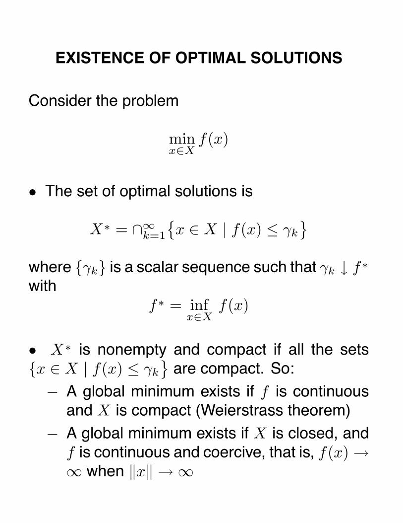
EXISTENCE OF OPTIMAL SOLUTIONS

Consider the problem

minx∈X

f(x)

• The set of optimal solutions is

X∗ = ∩∞k=1

{x ∈ X | f(x) ≤ γk

}where {γk} is a scalar sequence such that γk ↓ f∗

withf∗ = inf

x∈Xf(x)

• X∗ is nonempty and compact if all the sets{x ∈ X | f(x) ≤ γk

}are compact. So:

− A global minimum exists if f is continuousand X is compact (Weierstrass theorem)

− A global minimum exists if X is closed, andf is continuous and coercive, that is, f(x) →∞ when ‖x‖ → ∞

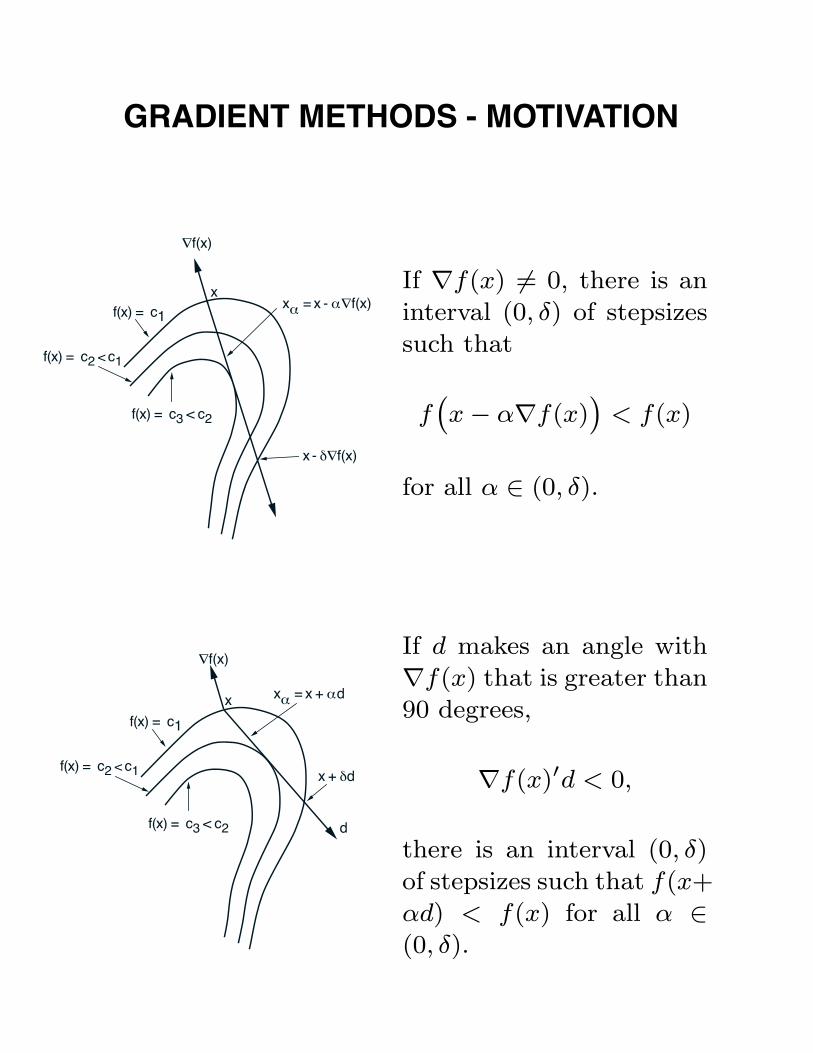
GRADIENT METHODS - MOTIVATION

f(x) = c1

f(x) = c2 < c1

f(x) = c3 < c2

xxα = x - α∇f(x)

∇f(x)

x - δ∇f(x)

If ∇f(x) �= 0, there is an

interval (0, δ) of stepsizes

such that

f(x − α∇f(x)

)< f(x)

for all α ∈ (0, δ).

f(x) = c1

f(x) = c2 < c1

f(x) = c3 < c2

x

∇f(x)

d

x + δd

xα = x + αd

If d makes an angle with

∇f(x) that is greater than

90 degrees,

∇f(x)′d < 0,

there is an interval (0, δ)

of stepsizes such that f(x+

αd) < f(x) for all α ∈(0, δ).

PRINCIPAL GRADIENT METHODS

xk+1 = xk + αkdk, k = 0, 1, . . .

where, if ∇f(xk) �= 0, the direction dk satisfies

∇f(xk)′dk < 0,

and αk is a positive stepsize. Principal example:

xk+1 = xk − αkDk∇f(xk),

where Dk is a positive definite symmetric matrix

• Simplest method: Steepest descent

xk+1 = xk − αk∇f(xk), k = 0, 1, . . .

• Most sophisticated method: Newton’s method

xk+1 = xk−αk(∇2f(xk)

)−1∇f(xk), k = 0, 1, . . .

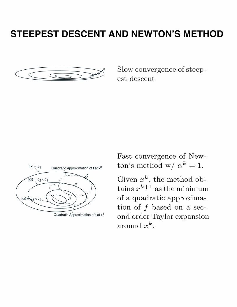
STEEPEST DESCENT AND NEWTON’S METHOD

x0 Slow convergence of steep-

est descent

x0

x1

x2

f(x) = c1

f(x) = c3 < c2

f(x) = c2 < c1.

.

.

Quadratic Approximation of f at x0

Quadratic Approximation of f at x1

Fast convergence of New-

ton’s method w/ αk = 1.

Given xk, the method ob-

tains xk+1 as the minimum

of a quadratic approxima-

tion of f based on a sec-

ond order Taylor expansion

around xk.

OTHER CHOICES OF DIRECTION

• Diagonally Scaled Steepest Descent

Dk = Diagonal approximation to(∇2f(xk)

)−1

• Modified Newton’s Method

Dk = (∇2f(x0))−1, k = 0, 1, . . . ,

• Discretized Newton’s Method

Dk =(H(xk)

)−1, k = 0, 1, . . . ,

where H(xk) is a finite-difference based approxi-mation of ∇2f(xk)

• Gauss-Newton method for least squares prob-lems: minx∈�n 1

2‖g(x)‖2. Here

Dk =(∇g(xk)∇g(xk)′

)−1, k = 0, 1, . . .


LECTURE 4

CONVERGENCE ANALYSIS OF GRADIENT METHODS

LECTURE OUTLINE

• Gradient Methods - Choice of Stepsize

• Gradient Methods - Convergence Issues

CHOICES OF STEPSIZE I

• Minimization Rule: αk is such that

f(xk + αkdk) = minα≥0

f(xk + αdk).

• Limited Minimization Rule: Min over α ∈ [0, s]

• Armijo rule:

σα∇f(xk)'dk

α∇f(xk)'dk

0 α

Set of AcceptableStepsizes

× ×s

×βs

Unsuccessful StepsizeTrials

β2sStepsize αk =

f(xk + αdk) - f(xk)

Start with s and continue with βs, β2s, ..., until βms falls

within the set of α with

f(xk) − f(xk + αdk) ≥ −σα∇f(xk)′dk.

CHOICES OF STEPSIZE II

• Constant stepsize: αk is such that

αk = s : a constant

• Diminishing stepsize:

αk → 0

but satisfies the infinite travel condition

∞∑k=0

αk = ∞

GRADIENT METHODS WITH ERRORS

xk+1 = xk − αk(∇f(xk) + ek)

where ek is an uncontrollable error vector

• Several special cases:

− ek small relative to the gradient; i.e., for allk, ‖ek‖ < ‖∇f(xk)‖

∇f(xk)

ek

gk

Illustration of the descent

property of the direction

gk = ∇f(xk) + ek.

− {ek} is bounded, i.e., for all k, ‖ek‖ ≤ δ,where δ is some scalar.

− {ek} is proportional to the stepsize, i.e., forall k, ‖ek‖ ≤ qαk, where q is some scalar.

− {ek} are independent zero mean random vec-tors

CONVERGENCE ISSUES

• Only convergence to stationary points can beguaranteed

• Even convergence to a single limit may be hardto guarantee (capture theorem)

• Danger of nonconvergence if directions dk tendto be orthogonal to ∇f(xk)

• Gradient related condition:

For any subsequence {xk}k∈K that converges toa nonstationary point, the corresponding subse-quence {dk}k∈K is bounded and satisfies

lim supk→∞, k∈K

∇f(xk)′dk < 0.

• Satisfied if dk = −Dk∇f(xk) and the eigenval-ues of Dk are bounded above and bounded awayfrom zero

CONVERGENCE RESULTS

CONSTANT AND DIMINISHING STEPSIZES

Let {xk} be a sequence generated by a gradientmethod xk+1 = xk +αkdk, where {dk} is gradientrelated. Assume that for some constant L > 0,we have

‖∇f(x) −∇f(y)‖ ≤ L‖x − y‖, ∀ x, y ∈ �n,

Assume that either

(1) there exists a scalar ε such that for all k

0 < ε ≤ αk ≤ (2 − ε)|∇f(xk)′dk|L‖dk‖2

or

(2) αk → 0 and∑∞

k=0 αk = ∞.

Then either f(xk) → −∞ or else {f(xk)} con-verges to a finite value and ∇f(xk) → 0.

MAIN PROOF IDEA

0 α

α∇f(xk)'dk + (1/2)α2L||dk||2

×

α∇f(xk)'dk

α = |∇f(xk)'dk|

L||dk||

|2

f(xk + αdk) - f(xk)

The idea of the convergence proof for a constant stepsize.

Given xk and the descent direction dk, the cost differ-

ence f(xk + αdk) − f(xk) is majorized by α∇f(xk)′dk +12α2L‖dk‖2 (based on the Lipschitz assumption; see next

slide). Minimization of this function over α yields the step-

size

α =|∇f(xk)′dk|

L‖dk‖2

This stepsize reduces the cost function f as well.

DESCENT LEMMA

Let α be a scalar and let g(α) = f(x + αy). Have

f(x + y) − f(x) = g(1) − g(0) =∫ 1

0

dg

dα(α) dα

=∫ 1

0

y′∇f(x + αy) dα

≤∫ 1

0

y′∇f(x) dα

+∣∣∣∣∫ 1

0

y′(∇f(x + αy) −∇f(x)

)dα

∣∣∣∣≤

∫ 1

0

y′∇f(x) dα

+∫ 1

0

‖y‖ · ‖∇f(x + αy) −∇f(x)‖dα

≤ y′∇f(x) + ‖y‖∫ 1

0

Lα‖y‖ dα

= y′∇f(x) +L

2‖y‖2.

CONVERGENCE RESULT – ARMIJO RULE

Let {xk} be generated by xk+1 = xk+αkdk, where{dk} is gradient related and αk is chosen by theArmijo rule. Then every limit point of {xk} is sta-tionary.

Proof Outline: Assume x is a nonstationary limitpoint. Then f(xk) → f(x), so αk∇f(xk)′dk → 0.

• If {xk}K → x, lim supk→∞, k∈K ∇f(xk)′dk < 0,by gradient relatedness, so that {αk}K → 0.

• By the Armijo rule, for large k ∈ K

f(xk)−f(xk +(αk/β)dk

)< −σ(αk/β)∇f(xk)′dk.

Defining pk = dk

‖dk‖ and αk = αk‖dk‖β , we have

f(xk) − f(xk + αkpk)αk

< −σ∇f(xk)′pk.

Use the Mean Value Theorem and let k → ∞.We get −∇f(x)′p ≤ −σ∇f(x)′p, where p is a limitpoint of pk – a contradiction since ∇f(x)′p < 0.


LECTURE 5: RATE OF CONVERGENCE

LECTURE OUTLINE

• Approaches for Rate of Convergence Analysis

• The Local Analysis Method

• Quadratic Model Analysis

• The Role of the Condition Number

• Scaling

• Diagonal Scaling

• Extension to Nonquadratic Problems

• Singular and Difficult Problems

APPROACHES FOR RATE OF

CONVERGENCE ANALYSIS

• Computational complexity approach

• Informational complexity approach

• Local analysis

• Why we will focus on the local analysis method

THE LOCAL ANALYSIS APPROACH

• Restrict attention to sequences xk convergingto a local min x∗

• Measure progress in terms of an error functione(x) with e(x∗) = 0, such as

e(x) = ‖x − x∗‖, e(x) = f(x) − f(x∗)

• Compare the tail of the sequence e(xk) with thetail of standard sequences

• Geometric or linear convergence [if e(xk) ≤ qβk

for some q > 0 and β ∈ [0, 1), and for all k]. Holdsif

lim supk→∞

e(xk+1)e(xk)

< β

• Superlinear convergence [if e(xk) ≤ q · βpk forsome q > 0, p > 1 and β ∈ [0, 1), and for all k].

• Sublinear convergence

QUADRATIC MODEL ANALYSIS

• Focus on the quadratic function f(x) = (1/2)x′Qx,with Q > 0.

• Analysis also applies to nonquadratic problemsin the neighborhood of a nonsingular local min

• Consider steepest descent

xk+1 = xk − αk∇f(xk) = (I − αkQ)xk

‖xk+1‖2 = xk′(I − αkQ)2xk

≤(max eig. (I − αkQ)2

)‖xk‖2

The eigenvalues of (I − αkQ)2 are equal to (1 −αkλi)2, where λi are the eigenvalues of Q, so

max eig of (I−αkQ)2 = max{(1−αkm)2, (1−αkM)2

}where m, M are the smallest and largest eigen-values of Q. Thus

‖xk+1‖‖xk‖ ≤ max

{|1 − αkm|, |1 − αkM |

}

OPTIMAL CONVERGENCE RATE

• The value of αk that minimizes the bound isα∗ = 2/(M + m), in which case

‖xk+1‖‖xk‖ ≤ M − m

M + m

0 α

1

|1 - αM |

|1 - αm |

max {|1 - αm|, |1 - αM|}

M - mM + m

2M + m

1M

1m

2M

Stepsizes thatGuarantee Convergence

• Conv. rate for minimization stepsize (see text)

f(xk+1)f(xk)

≤(

M − m

M + m

)2

• The ratio M/m is called the condition numberof Q, and problems with M/m: large are calledill-conditioned .

SCALING AND STEEPEST DESCENT

• View the more general method

xk+1 = xk − αkDk∇f(xk)

as a scaled version of steepest descent.

• Consider a change of variables x = Sy withS = (Dk)1/2. In the space of y, the problem is

minimize h(y) ≡ f(Sy)subject to y ∈ �n

• Apply steepest descent to this problem, multiplywith S, and pass back to the space of x, using∇h(yk) = S∇f(xk),

yk+1 = yk − αk∇h(yk)

Syk+1 = Syk − αkS∇h(yk)

xk+1 = xk − αkDk∇f(xk)

DIAGONAL SCALING

• Apply the results for steepest descent to thescaled iteration yk+1 = yk − αk∇h(yk):

‖yk+1‖‖yk‖ ≤ max

{|1 − αkmk|, |1 − αkMk|

}

f(xk+1)f(xk)

=h(yk+1)h(yk)

≤(

Mk − mk

Mk + mk

)2

where mk and Mk are the smallest and largesteigenvalues of the Hessian of h, which is

∇2h(y) = S∇2f(x)S = (Dk)1/2Q(Dk)1/2

• It is desirable to choose Dk as close as possibleto Q−1. Also if Dk is so chosen, the stepsize α = 1is near the optimal 2/(Mk + mk).

• Using as Dk a diagonal approximation to Q−1

is common and often very effective. Corrects forpoor choice of units expressing the variables.

NONQUADRATIC PROBLEMS

• Rate of convergence to a nonsingular local min-imum of a nonquadratic function is very similar tothe quadratic case (linear convergence is typical).

• If Dk →(∇2f(x∗)

)−1, we asymptotically obtain

optimal scaling and superlinear convergence

• More generally, if the direction dk = −Dk∇f(xk)approaches asymptotically the Newton direction,i.e.,

limk→∞

‖dk +(∇2f(x∗)

)−1∇f(xk)‖‖∇f(xk)‖ = 0

and the Armijo rule is used with initial stepsizeequal to one, the rate of convergence is superlin-ear.

• Convergence rate to a singular local min is typ-ically sublinear (in effect, condition number = ∞)


LECTURE 6

NEWTON AND GAUSS-NEWTON METHODS

LECTURE OUTLINE

• Newton’s Method

• Convergence Rate of the Pure Form

• Global Convergence

• Variants of Newton’s Method

• Least Squares Problems

• The Gauss-Newton Method

NEWTON’S METHOD

xk+1 = xk − αk(∇2f(xk)

)−1∇f(xk)

assuming that the Newton direction is defined andis a direction of descent

• Pure form of Newton’s method (stepsize = 1)

xk+1 = xk −(∇2f(xk)

)−1∇f(xk)

− Very fast when it converges (how fast?)

− May not converge (or worse, it may not bedefined) when started far from a nonsingularlocal min

− Issue: How to modify the method so thatit converges globally, while maintaining thefast convergence rate

CONVERGENCE RATE OF PURE FORM

• Consider solution of nonlinear system g(x) = 0where g : �n �→ �n, with method

xk+1 = xk −(∇g(xk)′

)−1g(xk)

− If g(x) = ∇f(x), we get pure form of Newton

• Quick derivation: Suppose xk → x∗ withg(x∗) = 0 and ∇g(x∗) is invertible. By Taylor

0 = g(x∗) = g(xk)+∇g(xk)′(x∗−xk)+o(‖xk−x∗‖

).

Multiply with(∇g(xk)′

)−1:

xk − x∗ −(∇g(xk)′

)−1g(xk) = o

(‖xk − x∗‖

),

soxk+1 − x∗ = o

(‖xk − x∗‖

),

implying superlinear convergence and capture.

CONVERGENCE BEHAVIOR OF PURE FORM

x0 = -1 x2 x1

x

k xk g(xk)

0 - 1.00000 - 0.632121 0.71828 1.050912 0.20587 0.228593 0.01981 0.020004 0.00019 0.000195 0.00000 0.00000

0

g(x) = ex - 1

g(x)

0

x

x0 x2x1x3

MODIFICATIONS FOR GLOBAL CONVERGENCE

• Use a stepsize

• Modify the Newton direction when:

− Hessian is not positive definite

− When Hessian is nearly singular (needed toimprove performance)

• Use

dk = −(∇2f(xk) + ∆k

)−1∇f(xk),

whenever the Newton direction does not exist oris not a descent direction. Here ∆k is a diagonalmatrix such that

∇2f(xk) + ∆k > 0

− Modified Cholesky factorization

− Trust region methods

LEAST-SQUARES PROBLEMS

minimize f(x) = 12‖g(x)‖2 = 1

2

m∑i=1

‖gi(x)‖2

subject to x ∈ �n,

where g = (g1, . . . , gm), gi : �n → �ri .

• Many applications:

− Solution of systems of n nonlinear equationswith n unknowns

− Model Construction – Curve Fitting

− Neural Networks

− Pattern Classification

PURE FORM OF THE GAUSS-NEWTON METHOD

• Idea: Linearize around the current point xk

g̃(x, xk) = g(xk) + ∇g(xk)′(x − xk)

and minimize the norm of the linearized functiong̃:

xk+1 = arg minx∈�n

12‖g̃(x, xk)‖2

= xk−(∇g(xk)∇g(xk)′

)−1∇g(xk)g(xk)

• The direction

−(∇g(xk)∇g(xk)′

)−1∇g(xk)g(xk)

is a descent direction since

∇g(xk)g(xk) = ∇((1/2)‖g(x)‖2

)∇g(xk)∇g(xk)′ > 0

MODIFICATIONS OF THE GAUSS-NEWTON

• Similar to those for Newton’s method:

xk+1 = xk−αk(∇g(xk)∇g(xk)′+∆k

)−1∇g(xk)g(xk)

where αk is a stepsize and ∆k is a diagonal matrixsuch that

∇g(xk)∇g(xk)′ + ∆k > 0

• Incremental version of the Gauss-Newton method:

− Operate in cycles

− Start a cycle with ψ0 (an estimate of x)

− Update ψ using a single component of g

ψi = arg minx∈�n

i∑j=1

‖g̃j(x, ψj−1)‖2, i = 1, . . . , m,

where g̃j are the linearized functions

g̃j(x, ψj−1) = gj(ψj−1)+∇gj(ψj−1)′(x−ψj−1)

MODEL CONSTRUCTION

• Given set of m input-output data pairs (yi, zi),i = 1, . . . , m, from the physical system

• Hypothesize an input/output relation z = h(x, y),where x is a vector of unknown parameters, andh is known

• Find x that matches best the data in the sensethat it minimizes the sum of squared errors

12

m∑i=1

‖zi − h(x, yi)‖2

• Example of a linear model: Fit the data pairs bya cubic polynomial approximation. Take

h(x, y) = x3y3 + x2y2 + x1y + x0,

where x = (x0, x1, x2, x3) is the vector of unknowncoefficients of the cubic polynomial.

NEURAL NETS

• Nonlinear model construction with multilayerperceptrons

• x of the vector of weights

• Universal approximation property

PATTERN CLASSIFICATION

• Objects are presented to us, and we wish toclassify them in one of s categories 1, . . . , s, basedon a vector y of their features.

• Classical maximum posterior probability ap-proach: Assume we know

p(j|y) = P (object w/ feature vector y is of category j)

Assign object with feature vector y to category

j∗(y) = arg maxj=1,...,s

p(j|y).

• If p(j|y) are unknown, we can estimate themusing functions hj(xj , y) parameterized by vectorsxj . Obtain xj by minimizing

12

m∑i=1

(zij − hj(xj , yi)

)2,

where

zij =

{1 if yi is of category j,0 otherwise.


LECTURE 7: ADDITIONAL METHODS

LECTURE OUTLINE

• Least-Squares Problems and Incremental Gra-dient Methods

• Conjugate Direction Methods

• The Conjugate Gradient Method

• Quasi-Newton Methods

• Coordinate Descent Methods

• Recall the least-squares problem:

minimize f(x) = 12‖g(x)‖2 = 1

2

m∑i=1

‖gi(x)‖2

subject to x ∈ �n,

where g = (g1, . . . , gm), gi : �n → �ri .

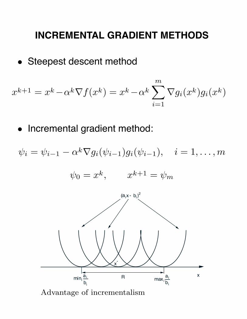
INCREMENTAL GRADIENT METHODS

• Steepest descent method

xk+1 = xk−αk∇f(xk) = xk−αk

m∑i=1

∇gi(xk)gi(xk)

• Incremental gradient method:

ψi = ψi−1 − αk∇gi(ψi−1)gi(ψi−1), i = 1, . . . , m

ψ0 = xk, xk+1 = ψm

(aix - bi )2

aminii

bi

amaxi

i

bi

x*

xR

Advantage of incrementalism

VIEW AS GRADIENT METHOD W/ ERRORS

• Can write incremental gradient method as

xk+1 = xk − αk

m∑i=1

∇gi(xk)gi(xk)

+ αk

m∑i=1

(∇gi(xk)gi(xk) −∇gi(ψi−1)gi(ψi−1)

)

• Error term is proportional to stepsize αk

• Convergence (generically) for a diminishing step-size (under a Lipschitz condition on ∇gigi)

• Convergence to a “neighborhood” for a constantstepsize

CONJUGATE DIRECTION METHODS

• Aim to improve convergence rate of steepest de-scent, without the overhead of Newton’s method.

• Analyzed for a quadratic model. They require niterations to minimize f(x) = (1/2)x′Qx−b′x withQ an n × n positive definite matrix Q > 0.

• Analysis also applies to nonquadratic problemsin the neighborhood of a nonsingular local min.

• The directions d1, . . . , dk are Q-conjugate if di′Qdj =0 for all i �= j.

• Generic conjugate direction method:

xk+1 = xk + αkdk

where αk is obtained by line minimization.

y0

y1

y2

w0

w1

x0 x1

x2

d1 = Q-1/2w1

d0 = Q-1/2w0

Expanding Subspace Theorem

GENERATING Q-CONJUGATE DIRECTIONS

• Given set of linearly independent vectors ξ0, . . . , ξk,we can construct a set of Q-conjugate directionsd0, . . . , dk s.t. Span(d0, . . . , di) = Span(ξ0, . . . , ξi)

• Gram-Schmidt procedure. Start with d0 = ξ0.If for some i < k, d0, . . . , di are Q-conjugate andthe above property holds, take

di+1 = ξi+1 +i∑

m=0

c(i+1)mdm;

choose c(i+1)m so di+1 is Q-conjugate to d0, . . . , di,

di+1′Qdj = ξi+1′Qdj+

(i∑

m=0

c(i+1)mdm

)′

Qdj = 0.

ξ0 = d0- c10d0

ξ1 ξ2

d1

d00

0

d1= ξ1 + c10d0

d2= ξ2 + c20d0 + c21d1

CONJUGATE GRADIENT METHOD

• Apply Gram-Schmidt to the vectors ξk = −gk =−∇f(xk), k = 0, 1, . . . , n − 1. Then

dk = −gk +k−1∑j=0

gk′Qdj

dj ′Qdjdj

• Key fact: Direction formula can be simplified.

Proposition : The directions of the CGM aregenerated by d0 = −g0, and

dk = −gk + βkdk−1, k = 1, . . . , n − 1,

where βk is given by

βk =gk′gk

gk−1′gk−1or βk =

(gk − gk−1)′gk

gk−1′gk−1

Furthermore, the method terminates with an opti-mal solution after at most n steps.

• Extension to nonquadratic problems.

PROOF OF CONJUGATE GRADIENT RESULT

• Use induction to show that all gradients gk gen-erated up to termination are linearly independent.True for k = 1. Suppose no termination after ksteps, and g0, . . . , gk−1 are linearly independent.Then, Span(d0, . . . , dk−1) = Span(g0, . . . , gk−1)and there are two possibilities:

− gk = 0, and the method terminates.

− gk �= 0, in which case from the expandingmanifold property

gk is orthogonal to d0, . . . , dk−1

gk is orthogonal to g0, . . . , gk−1

so gk is linearly independent of g0, . . . , gk−1,completing the induction.

• Since at most n lin. independent gradients canbe generated, gk = 0 for some k ≤ n.

• Algebra to verify the direction formula.

QUASI-NEWTON METHODS

• xk+1 = xk − αkDk∇f(xk), where Dk is aninverse Hessian approximation.

• Key idea: Successive iterates xk, xk+1 and gra-dients ∇f(xk), ∇f(xk+1), yield curvature info

qk ≈ ∇2f(xk+1)pk,

pk = xk+1 − xk, qk = ∇f(xk+1) −∇f(xk),

∇2f(xn) ≈[q0 · · · qn−1

][p0 · · · pn−1

]−1

• Most popular Quasi-Newton method is a cleverway to implement this idea

Dk+1 = Dk +pkpk′

pk′qk− Dkqkqk′Dk

qk′Dkqk+ ξkτkvkvk′,

vk =pk

pk′qk−Dkqk

τk, τk = qk′Dkqk, 0 ≤ ξk ≤ 1

and D0 > 0 is arbitrary, αk by line minimization,and Dn = Q−1 for a quadratic.

NONDERIVATIVE METHODS

• Finite difference implementations

• Forward and central difference formulas

∂f(xk)∂xi

≈ 1h

(f(xk + hei) − f(xk)

)∂f(xk)

∂xi≈ 1

2h

(f(xk + hei) − f(xk − hei)

)• Use central difference for more accuracy nearconvergence

xk

xk+1xk+2

• Coordinate descent.Applies also to the casewhere there are boundconstraints on the vari-ables.

• Direct search methods. Nelder-Mead method.


LECTURE 8

OPTIMIZATION OVER A CONVEX SET;


Problem: minx∈X f(x), where:

(a) X ⊂ �n is nonempty, convex, and closed.

(b) f is continuously differentiable over X.

• Local and global minima. If f is convex localminima are also global.

f(x)

x

Local Minima Global Minimum

X

OPTIMALITY CONDITION

Proposition (Optimality Condition)

(a) If x∗ is a local minimum of f over X, then

∇f(x∗)′(x − x∗) ≥ 0, ∀ x ∈ X.

(b) If f is convex over X, then this condition isalso sufficient for x∗ to minimize f over X.

Surfaces of equal cost f(x)

Constraint set X

x

x*

∇f(x*)At a local minimum x∗,

the gradient ∇f(x∗) makes

an angle less than or equal

to 90 degrees with all fea-

sible variations x−x∗, x ∈X.

Constraint set X

x*

x

∇f(x*)Illustration of failure of the

optimality condition when

X is not convex. Here x∗

is a local min but we have

∇f(x∗)′(x − x∗) < 0 for

the feasible vector x shown.

PROOF

Proof: (a) By contradiction. Suppose that∇f(x∗)′(x−x∗) < 0 for some x ∈ X. By the Mean Value The-orem, for every ε > 0 there exists an s ∈ [0, 1]such that

f(x∗+ε(x−x∗)

)= f(x∗)+ε∇f

(x∗+sε(x−x∗)

)′(x−x∗).

Since ∇f is continuous, for suff. small ε > 0,

∇f(x∗ + sε(x − x∗)

)′(x − x∗) < 0

so that f(x∗ + ε(x − x∗)

)< f(x∗). The vector

x∗ + ε(x − x∗) is feasible for all ε ∈ [0, 1] becauseX is convex, so the optimality of x∗ is contradicted.

(b) Using the convexity of f

f(x) ≥ f(x∗) + ∇f(x∗)′(x − x∗)

for every x ∈ X. If the condition∇f(x∗)′(x−x∗) ≥0 holds for all x ∈ X, we obtain f(x) ≥ f(x∗), sox∗ minimizes f over X. Q.E.D.

OPTIMIZATION SUBJECT TO BOUNDS

• Let X = {x | x ≥ 0}. Then the necessarycondition for x∗ = (x∗

1, . . . , x∗n) to be a local min is

n∑i=1

∂f(x∗)

∂xi(xi − x∗

i ) ≥ 0, ∀ xi ≥ 0, i = 1, . . . , n.

• Fix i. Let xj = x∗j for j �= i and xi = x∗

i + 1:

∂f(x∗)∂xi

≥ 0, ∀ i.

• If x∗i > 0, let also xj = x∗

j for j �= i and xi = 12x∗

i .Then ∂f(x∗)/∂xi ≤ 0, so

∂f(x∗)∂xi

= 0, if x∗i > 0.

x* x* = 0

∇f(x*)∇f(x*)

OPTIMIZATION OVER A SIMPLEX

X =

{x

∣∣∣ x ≥ 0,n∑

i=1

xi = r

}

where r > 0 is a given scalar.

• Necessary condition for x∗ = (x∗1, . . . , x

∗n) to be

a local min:

n∑i=1

∂f(x∗)

∂xi(xi−x∗

i ) ≥ 0, ∀ xi ≥ 0 with

n∑i=1

xi = r.

• Fix i with x∗i > 0 and let j be any other index.

Use x with xi = 0, xj = x∗j + x∗

i , and xm = x∗m for

all m �= i, j:

(∂f(x∗)

∂xj− ∂f(x∗)

∂xi

)x∗

i ≥ 0,

x∗i > 0 =⇒ ∂f(x∗)

∂xi≤ ∂f(x∗)

∂xj, ∀ j,

i.e., at the optimum, positive components haveminimal (and equal) first cost derivative.

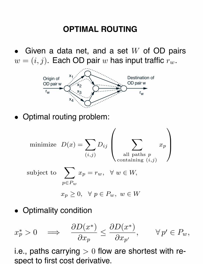
OPTIMAL ROUTING

• Given a data net, and a set W of OD pairsw = (i, j). Each OD pair w has input traffic rw.

Origin of OD pair w

Destination of OD pair w

rw rw

x1

x4

x3

x2

• Optimal routing problem:

minimize D(x) =∑(i,j)

Dij

⎛⎜⎝ ∑

all paths pcontaining (i,j)

xp

⎞⎟⎠

subject to∑

p∈Pw

xp = rw, ∀ w ∈ W,

xp ≥ 0, ∀ p ∈ Pw, w ∈ W

• Optimality condition

x∗p > 0 =⇒ ∂D(x∗)

∂xp≤ ∂D(x∗)

∂xp′, ∀ p′ ∈ Pw,

i.e., paths carrying > 0 flow are shortest with re-spect to first cost derivative.

TRAFFIC ASSIGNMENT

• Transportation network with OD pairs w. Eachw has paths p ∈ Pw and traffic rw. Let xp be the

flow of path p and let Tij

(∑p: crossing (i,j)

xp

)be the travel time of link (i, j).

• User-optimization principle: Traffic equilib-rium is established when each user of the networkchooses, among all available paths, a path of min-imum travel time, i.e., for all w ∈ W and pathsp ∈ Pw,

x∗p > 0 =⇒ tp(x

∗) ≤ tp′(x∗), ∀ p′ ∈ Pw, ∀ w ∈ W

where tp(x), is the travel time of path p

tp(x) =∑

all arcs (i,j)on path p

Tij(Fij), ∀ p ∈ Pw, ∀ w ∈ W.

Identical with the optimality condition of the routingproblem if we identify the arc travel time Tij(Fij)with the cost derivative D′

ij(Fij).

PROJECTION OVER A CONVEX SET

• Let z ∈ �n and a closed convex set X be given.Problem:

minimize f(x) = ‖z − x‖2

subject to x ∈ X.

Proposition (Projection Theorem) Problemhas a unique solution [z]+ (the projection of z).

z

x

Constraint set X

x*

x - x*

z - x*

Necessary and sufficient con-

dition for x∗ to be the pro-

jection. The angle between

z − x∗ and x − x∗ should

be greater or equal to 90

degrees for all x ∈ X, or

(z − x∗)′(x − x∗) ≤ 0

• If X is a subspace, z − x∗ ⊥ X.

• The mapping f : �n �→ X defined by f(x) =[x]+ is continuous and nonexpansive, that is,

‖[x]+ − [y]+‖ ≤ ‖x − y‖, ∀ x, y ∈ �n.


LECTURE 9: FEASIBLE DIRECTION METHODS

LECTURE OUTLINE

• Conditional Gradient Method

• Gradient Projection Methods

A feasible direction at an x ∈ X is a vector d �= 0such that x+αd is feasible for all suff. small α > 0

x1

x2

d

Constraint set X

Feasible directions at x

x

• Note: the set of feasible directions at x is theset of all α(z − x) where z ∈ X, z �= x, and α > 0

FEASIBLE DIRECTION METHODS

• A feasible direction method:

xk+1 = xk + αkdk,

where dk: feasible descent direction [∇f(xk)′dk <0], and αk > 0 and such that xk+1 ∈ X.

• Alternative definition:

xk+1 = xk + αk(xk − xk),

where αk ∈ (0, 1] and if xk is nonstationary,

xk ∈ X, ∇f(xk)′(xk − xk) < 0.

• Stepsize rules: Limited minimization, Constantαk = 1, Armijo: αk = βmk , where mk is the firstnonnegative m for which

f(xk)−f(xk+βm(xk−xk)

)≥ −σβm∇f(xk)′(xk−xk)

CONVERGENCE ANALYSIS

• Similar to the one for (unconstrained) gradientmethods.

• The direction sequence {dk} is gradient relatedto {xk} if the following property can be shown:For any subsequence {xk}k∈K that converges toa nonstationary point, the corresponding subse-quence {dk}k∈K is bounded and satisfies


∇f(xk)′dk < 0.

Proposition (Stationarity of Limit Points)Let {xk} be a sequence generated by the feasibledirection method xk+1 = xk +αkdk. Assume that:

− {dk} is gradient related

− αk is chosen by the limited minimization ruleor the Armijo rule.

Then every limit point of {xk} is a stationary point.

• Proof: Nearly identical to the unconstrainedcase.

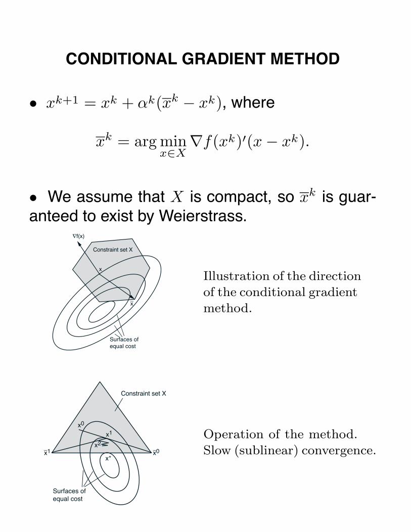
CONDITIONAL GRADIENT METHOD

• xk+1 = xk + αk(xk − xk), where

xk = arg minx∈X

∇f(xk)′(x − xk).

• We assume that X is compact, so xk is guar-anteed to exist by Weierstrass.

∇f(x)

x

x_

Constraint set X

Surfaces ofequal cost

Illustration of the direction

of the conditional gradient

method.

x0

x1

x2

x1 x0__

Constraint set X

Surfaces ofequal cost

x*

Operation of the method.

Slow (sublinear) convergence.

CONVERGENCE OF CONDITIONAL GRADIENT

• Show that the direction sequence of the condi-tional gradient method is gradient related, so thegeneric convergence result applies.

• Suppose that {xk}k∈K converges to a nonsta-tionary point x̃. We must prove that

{xk−xk}k∈K : bounded, lim supk→∞, k∈K

∇f(xk)′(xk−xk) < 0

• 1st relation: Holds because xk ∈ X, xk ∈ X,and X is assumed compact.

• 2nd relation: Note that by definition of xk,

∇f(xk)′(xk−xk) ≤ ∇f(xk)′(x−xk), ∀ x ∈ X

Taking limit as k → ∞, k ∈ K, and min of the RHSover x ∈ X, and using the nonstationarity of x̃,


∇f(xk)′(xk−xk) ≤ minx∈X

∇f(x̃)′(x−x̃) < 0,

thereby proving the 2nd relation.

GRADIENT PROJECTION METHODS

• Gradient projection methods determine the fea-sible direction by using a quadratic cost subprob-lem. Simplest variant:

xk+1 = xk + αk(xk − xk)

xk =[xk − sk∇f(xk)

]+where, [·]+ denotes projection on the set X, αk ∈(0, 1] is a stepsize, and sk is a positive scalar.

Constraint set X

xk

xk+1 = xk - sk∇f(xk)

xk+1 - sk+1∇f(xk+1)

xk+2 - sk+2∇f(xk+2)

xk+2

xk+1

xk+3

Gradient projection itera-

tions for the case

αk ≡ 1, xk+1 ≡ xk

If αk < 1, xk+1 is in the

line segment connecting xk

and xk.

• Stepsize rules for αk (assuming sk ≡ s): Limitedminimization, Armijo along the feasible direction,constant stepsize. Also, Armijo along the projec-tion arc (αk ≡ 1, sk: variable).

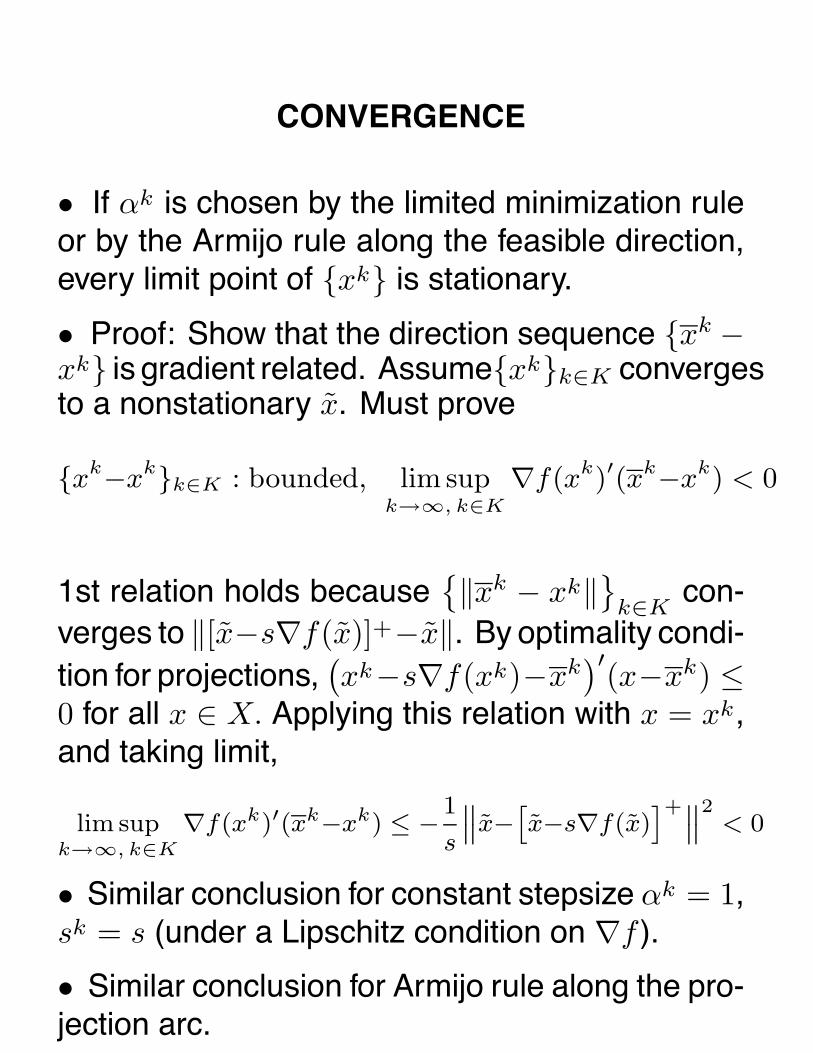
CONVERGENCE

• If αk is chosen by the limited minimization ruleor by the Armijo rule along the feasible direction,every limit point of {xk} is stationary.

• Proof: Show that the direction sequence {xk −xk} is gradient related. Assume{xk}k∈K convergesto a nonstationary x̃. Must prove

{xk−xk}k∈K : bounded, lim supk→∞, k∈K

∇f(xk)′(xk−xk) < 0

1st relation holds because{‖xk − xk‖

}k∈K

con-verges to ‖[x̃−s∇f(x̃)]+−x̃‖. By optimality condi-tion for projections,

(xk−s∇f(xk)−xk

)′(x−xk) ≤0 for all x ∈ X. Applying this relation with x = xk,and taking limit,


∇f(xk)′(xk−xk) ≤ −1

s

∥∥x̃−[x̃−s∇f(x̃)

]+∥∥2< 0

• Similar conclusion for constant stepsize αk = 1,sk = s (under a Lipschitz condition on ∇f ).

• Similar conclusion for Armijo rule along the pro-jection arc.

CONVERGENCE RATE – VARIANTS

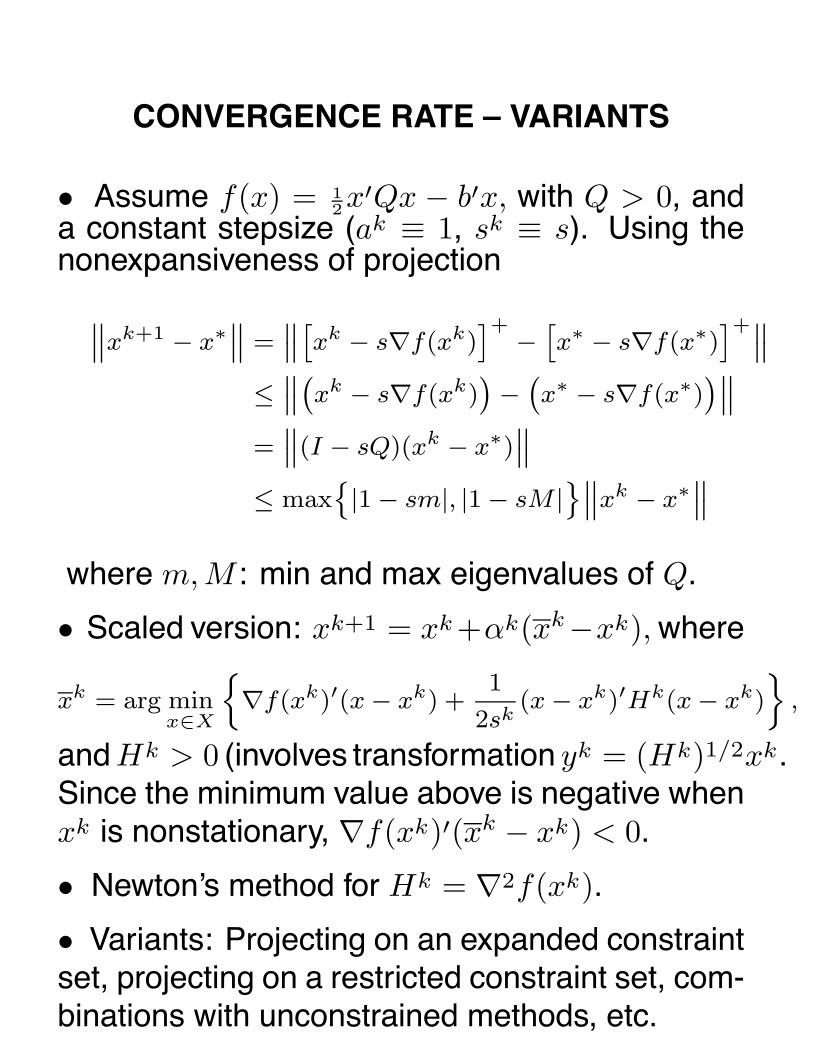
• Assume f(x) = 12x

′Qx − b′x, with Q > 0, anda constant stepsize (ak ≡ 1, sk ≡ s). Using thenonexpansiveness of projection

∥∥xk+1 − x∗∥∥ =

∥∥[xk − s∇f(xk)

]+−

[x∗ − s∇f(x∗)

]+∥∥≤

∥∥(xk − s∇f(xk)

)−

(x∗ − s∇f(x∗)

)∥∥=

∥∥(I − sQ)(xk − x∗)∥∥

≤ max{|1 − sm|, |1 − sM |

}∥∥xk − x∗∥∥

where m, M : min and max eigenvalues of Q.

• Scaled version: xk+1 = xk +αk(xk−xk), where

xk = arg minx∈X

{∇f(xk)′(x − xk) +

1

2sk(x − xk)′Hk(x − xk)

},

and Hk > 0 (involves transformation yk = (Hk)1/2xk.Since the minimum value above is negative whenxk is nonstationary, ∇f(xk)′(xk − xk) < 0.

• Newton’s method for Hk = ∇2f(xk).

• Variants: Projecting on an expanded constraintset, projecting on a restricted constraint set, com-binations with unconstrained methods, etc.


LECTURE 10

ALTERNATIVES TO GRADIENT PROJECTION

LECTURE OUTLINE

• Three Alternatives/Remedies for Gradient Pro-jection

− Two-Metric Projection Methods

− Manifold Suboptimization Methods

− Affine Scaling Methods

Scaled GP method with scaling matrix Hk > 0:

xk+1 = xk + αk(xk − xk),

xk = arg minx∈X

{∇f(xk)′(x − xk) +

1


}.

• The QP direction subproblem is complicated by:

− Difficult inequality (e.g., nonorthant) constraints

− Nondiagonal Hk, needed for Newton scaling

THREE WAYS TO DEAL W/ THE DIFFICULTY

• Two-metric projection methods:

xk+1 =[xk − αkDk∇f(xk)

]+− Use Newton-like scaling but use a standard

projection

− Suitable for bounds, simplexes, Cartesianproducts of simple sets, etc

• Manifold suboptimization methods:

− Use (scaled) gradient projection on the man-ifold of active inequality constraints

− Each QP subproblem is equality-constrained

− Need strategies to cope with changing activemanifold (add-drop constraints)

• Affine Scaling Methods

− Go through the interior of the feasible set

− Each QP subproblem is equality-constrained,AND we don’t have to deal with changing ac-tive manifold

TWO-METRIC PROJECTION METHODS

• In their simplest form, apply to constraint: x ≥ 0,but generalize to bound and other constraints

• Like unconstr. gradient methods except for [·]+

xk+1 =[xk − αkDk∇f(xk)

]+, Dk > 0

• Major difficulty: Descent is not guaranteed forDk: arbitrary

∇f(xk)

xk

xk - αkDk∇f(xk)

xk

xk - αkDk∇f(xk)

(a) (b)

• Remedy: Use Dk that is diagonal w/ respect toindices that “are active and want to stay active”

I+(xk) ={

i∣∣∣ xk

i = 0, ∂f(xk)/∂xi > 0}

PROPERTIES OF 2-METRIC PROJECTION

• Suppose Dk is diagonal with respect to I+(xk),i.e., dk

ij = 0 for i, j ∈ I+(xk) with i �= j, and let

xk(a) =[xk − αDk∇f(xk)

]+− If xk is stationary, xk = xk(α) for all α > 0.

− Otherwise f(x(α)

)< f(xk) for all sufficiently

small α > 0 (can use Armijo rule).

• Because I+(x) is discontinuous w/ respect tox, to guarantee convergence we need to includein I+(x) constraints that are “ε-active” [those w/xk

i ∈ [0, ε] and ∂f(xk)/∂xi > 0].

• The constraints in I+(x∗) eventually becomeactive and don’t matter.

• Method reduces to unconstrained Newton-likemethod on the manifold of active constraints at x∗.

• Thus, superlinear convergence is possible w/simple projections.

MANIFOLD SUBOPTIMIZATION METHODS

• Feasible direction methods for

min f(x) subject to a′jx ≤ bj , j = 1, . . . , r

• Gradient is projected on a linear manifold of ac-tive constraints rather than on the entire constraintset (linearly constrained QP).

x0

x1

x2

x3

(a)

x0

x4

x2

x1

(b)

x3

• Searches through sequence of manifolds, eachdiffering by at most one constraint from the next.

• Potentially many iterations to identify the activemanifold; then method reduces to (scaled) steep-est descent on the active manifold.

• Well-suited for a small number of constraints,and for quadratic programming.

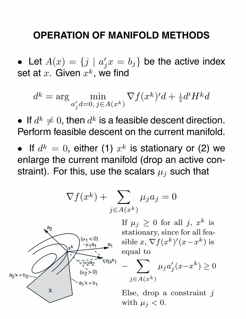
OPERATION OF MANIFOLD METHODS

• Let A(x) = {j | a′jx = bj} be the active index

set at x. Given xk, we find

dk = arg mina′

jd=0, j∈A(xk)

∇f(xk)′d + 12d

′Hkd

• If dk �= 0, then dk is a feasible descent direction.Perform feasible descent on the current manifold.

• If dk = 0, either (1) xk is stationary or (2) weenlarge the current manifold (drop an active con-straint). For this, use the scalars µj such that

∇f(xk) +∑

j∈A(xk)

µjaj = 0

∇f(xk)

a1

a2

X

a1'x = b1

a2'x = b2

- µ2a2

- µ1a1

(µ1 < 0)

(µ2 > 0)

xk

If µj ≥ 0 for all j, xk is

stationary, since for all fea-

sible x, ∇f(xk)′(x−xk) is

equal to

−∑

j∈A(xk)

µja′j(x−xk) ≥ 0

Else, drop a constraint j

with µj < 0.

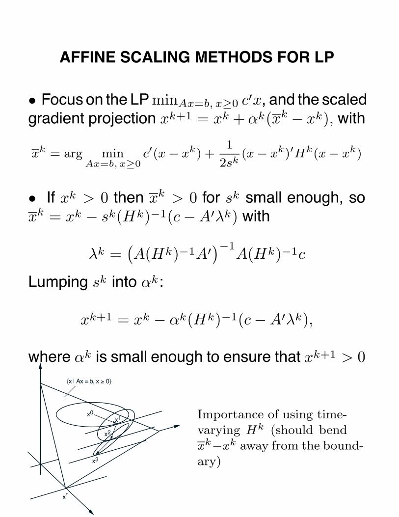
AFFINE SCALING METHODS FOR LP

• Focus on the LP minAx=b, x≥0 c′x, and the scaledgradient projection xk+1 = xk + αk(xk − xk), with

xk = arg minAx=b, x≥0

c′(x − xk) +1


• If xk > 0 then xk > 0 for sk small enough, soxk = xk − sk(Hk)−1(c − A′λk) with

λk =(A(Hk)−1A′

)−1A(Hk)−1c

Lumping sk into αk:

xk+1 = xk − αk(Hk)−1(c − A′λk),

where αk is small enough to ensure that xk+1 > 0

x*

x1

x2

x3

x0

{x | Ax = b, x ≥ 0}

Importance of using time-

varying Hk (should bend

xk−xk away from the bound-

ary)

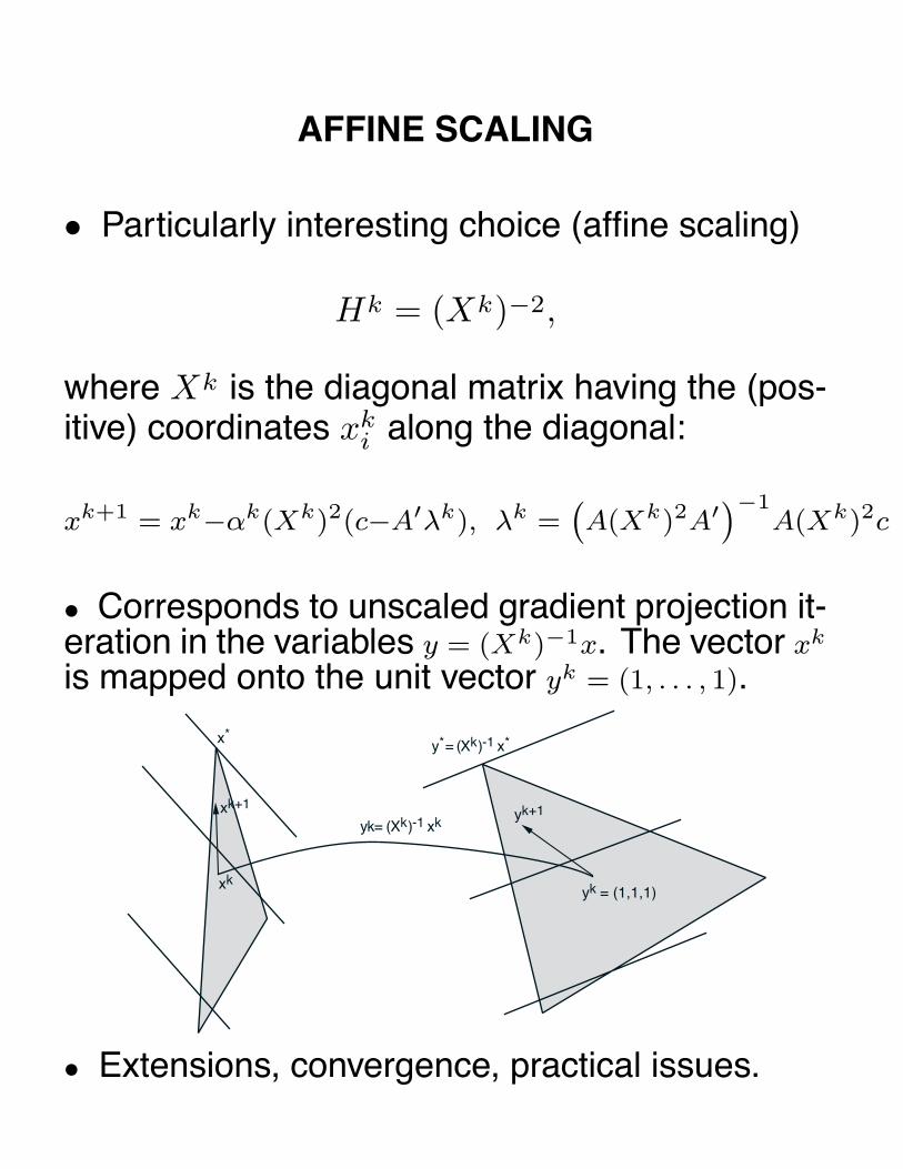
AFFINE SCALING

• Particularly interesting choice (affine scaling)

Hk = (Xk)−2,

where Xk is the diagonal matrix having the (pos-itive) coordinates xk

i along the diagonal:

xk+1 = xk−αk(Xk)2(c−A′λk), λk =(A(Xk)2A′)−1

A(Xk)2c

• Corresponds to unscaled gradient projection it-eration in the variables y = (Xk)−1x. The vector xk

is mapped onto the unit vector yk = (1, . . . , 1).

x*

xk

xk+1yk+1

yk = (1,1,1)

y*= (Xk)-1 x*

yk= (Xk)-1 xk

• Extensions, convergence, practical issues.


LECTURE 11

CONSTRAINED OPTIMIZATION;

LAGRANGE MULTIPLIERS

LECTURE OUTLINE

• Equality Constrained Problems

• Basic Lagrange Multiplier Theorem

• Proof 1: Elimination Approach

• Proof 2: Penalty Approach

Equality constrained problem

minimize f(x)

subject to hi(x) = 0, i = 1, . . . , m.

where f : �n �→ �, hi : �n �→ �, i = 1, . . . , m, are con-tinuously differentiable functions. (Theory alsoapplies to case where f and hi are cont. differ-entiable in a neighborhood of a local minimum.)

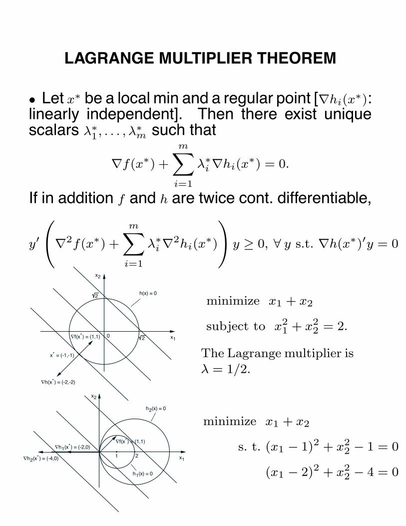
LAGRANGE MULTIPLIER THEOREM

• Let x∗ be a local min and a regular point [∇hi(x∗):

linearly independent]. Then there exist uniquescalars λ∗

1, . . . , λ∗m such that

∇f(x∗) +

m∑i=1

λ∗i ∇hi(x

∗) = 0.

If in addition f and h are twice cont. differentiable,

y′

(∇2f(x∗) +

m∑i=1

λ∗i ∇2hi(x

∗)

)y ≥ 0, ∀ y s.t. ∇h(x∗)′y = 0

x1

x2

x* = (-1,-1)

∇h(x*) = (-2,-2)

∇f(x*) = (1,1) 0

2

2

h(x) = 0

minimize x1 + x2

subject to x21 + x2

2 = 2.

The Lagrange multiplier is

λ = 1/2.

x1

x2

∇f(x*) = (1,1)∇h1(x*) = (-2,0)

∇h2(x*) = (-4,0)

h1(x) = 0

h2(x) = 0

21

minimize x1 + x2

s. t. (x1 − 1)2 + x22 − 1 = 0

(x1 − 2)2 + x22 − 4 = 0

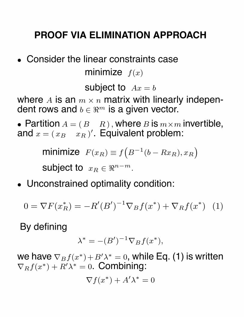
PROOF VIA ELIMINATION APPROACH

• Consider the linear constraints caseminimize f(x)

subject to Ax = b

where A is an m × n matrix with linearly indepen-dent rows and b ∈ �m is a given vector.

• Partition A = ( B R ) , where B is m×m invertible,and x = ( xB xR )′. Equivalent problem:

minimize F (xR) ≡ f(B−1(b − RxR), xR

)subject to xR ∈ �n−m.

• Unconstrained optimality condition:

0 = ∇F (x∗R) = −R′(B′)−1∇Bf(x∗) + ∇Rf(x∗) (1)

By definingλ∗ = −(B′)−1∇Bf(x∗),

we have ∇Bf(x∗)+B′λ∗ = 0, while Eq. (1) is written∇Rf(x∗) + R′λ∗ = 0. Combining:

∇f(x∗) + A′λ∗ = 0

ELIMINATION APPROACH - CONTINUED

• Second order condition: For all d ∈ �n−m

0 ≤ d′∇2F (x∗R)d = d′∇2

(f(B−1(b − RxR), xR

))d. (2)

• After calculation we obtain

∇2F (x∗R) = R′(B′)−1∇2

BBf(x∗)B−1R

− R′(B′)−1∇2BRf(x∗) −∇2

RBf(x∗)B−1R + ∇2RRf(x∗).

• Eq. (2) and the linearity of the constraints [im-plying that ∇2hi(x

∗) = 0], yields for all d ∈ �n−m

0 ≤ d′∇2F (x∗R)d = y′∇2f(x∗)y

= y′

(∇2f(x∗) +

m∑i=1

λ∗i ∇2hi(x

∗)

)y,

where y = ( yB yR )′ = (−B−1Rd d )′ .

• y has this form iff

0 = ByB + RyR = ∇h(x∗)′y.

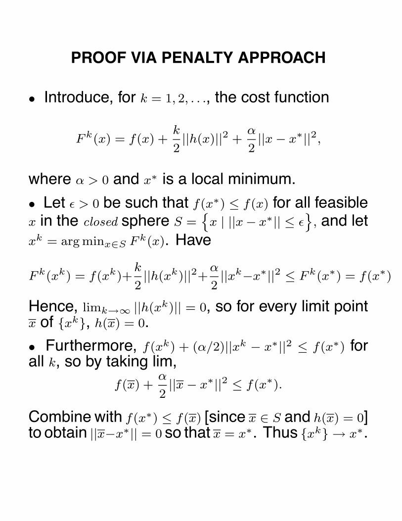
PROOF VIA PENALTY APPROACH

• Introduce, for k = 1, 2, . . ., the cost function

F k(x) = f(x) +k

2||h(x)||2 +

α

2||x − x∗||2,

where α > 0 and x∗ is a local minimum.

• Let ε > 0 be such that f(x∗) ≤ f(x) for all feasiblex in the closed sphere S =

{x | ||x − x∗|| ≤ ε

}, and let

xk = arg minx∈S F k(x). Have

F k(xk) = f(xk)+k

2||h(xk)||2+

α

2||xk−x∗||2 ≤ F k(x∗) = f(x∗)

Hence, limk→∞ ||h(xk)|| = 0, so for every limit pointx of {xk}, h(x) = 0.

• Furthermore, f(xk) + (α/2)||xk − x∗||2 ≤ f(x∗) forall k, so by taking lim,

f(x) +α

2||x − x∗||2 ≤ f(x∗).

Combine with f(x∗) ≤ f(x) [since x ∈ S and h(x) = 0]to obtain ||x−x∗|| = 0 so that x = x∗. Thus {xk} → x∗.

PENALTY APPROACH - CONTINUED

• Since xk → x∗, for large k, xk is interior to S, andis an unconstrained local minimum of F k(x).

• From 1st order necessary condition,

0 = ∇F k(xk) = ∇f(xk)+k∇h(xk)h(xk)+α(xk−x∗). (3)

Since ∇h(x∗) has rank m, ∇h(xk) also has rankm for large k, so ∇h(xk)′∇h(xk): invertible. Thus,multiplying Eq. (3) w/ ∇h(xk)′

kh(xk) = −(∇h(xk)′∇h(xk)

)−1∇h(xk)′

(∇f(xk)+α(xk−x∗)

).

Taking limit as k → ∞ and xk → x∗,

{kh(xk)

}→ −

(∇h(x∗)′∇h(x∗)

)−1∇h(x∗)′∇f(x∗) ≡ λ∗.

Taking limit as k → ∞ in Eq. (3), we obtain

∇f(x∗) + ∇h(x∗)λ∗ = 0.

• 2nd order L-multiplier condition: Use 2nd orderunconstrained condition for xk, and algebra.

LAGRANGIAN FUNCTION

• Define the Lagrangian function

L(x, λ) = f(x) +

m∑i=1

λihi(x).

Then, if x∗ is a local minimum which is regular, theLagrange multiplier conditions are written

∇xL(x∗, λ∗) = 0, ∇λL(x∗, λ∗) = 0,

System of n + m equations with n + m unknowns.

y′∇2xxL(x∗, λ∗)y ≥ 0, ∀ y s.t. ∇h(x∗)′y = 0.

• Exampleminimize 1

2

(x21 + x2

2 + x23

)subject to x1 + x2 + x3 = 3.

Necessary conditions

x∗1 + λ∗ = 0, x∗

2 + λ∗ = 0,

x∗3 + λ∗ = 0, x∗

1 + x∗2 + x∗

3 = 3.

EXAMPLE - PORTFOLIO SELECTION

• Investment of 1 unit of wealth among n assetswith random rates of return ei, and given meansei, and covariance matrix Q =

[E{(ei −ei)(ej −ej)}

].

• If xi: amount invested in asset i, we want to

minimize x′Qx

(= Variance of return

∑i

eixi

)subject to

∑ixi = 1, and a given mean

∑i

eixi = m

• Let λ1 and λ2 be the L-multipliers. Have 2Qx∗ +

λ1u+λ2e = 0, where u = (1, . . . , 1)′ and e = (e1, . . . , en)′.This yields

x∗ = mv+w, Variance of return = σ2 = (αm+β)2+γ,

where v and w are vectors, and α, β, and γ aresome scalars that depend on Q and e.

m

σ

ef-

Efficient Frontier σ = αm + β

For given m the optimal σ

lies on a line (called “effi-

cient frontier”).


LECTURE 12: SUFFICIENCY CONDITIONS

LECTURE OUTLINE

• Equality Constrained Problems/Sufficiency Con-ditions

• Convexification Using Augmented Lagrangians

• Proof of the Sufficiency Conditions

• Sensitivity

Equality constrained problem

minimize f(x)

subject to hi(x) = 0, i = 1, . . . , m.

where f : �n �→ �, hi : �n �→ �, are continuouslydifferentiable. To obtain sufficiency conditions, as-sume that f and hi are twice continuously differen-tiable.

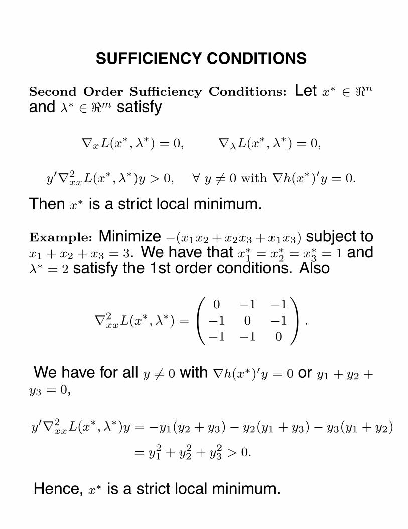
SUFFICIENCY CONDITIONS

Second Order Sufficiency Conditions: Let x∗ ∈ �n

and λ∗ ∈ �m satisfy

∇xL(x∗, λ∗) = 0, ∇λL(x∗, λ∗) = 0,

y′∇2xxL(x∗, λ∗)y > 0, ∀ y �= 0 with ∇h(x∗)′y = 0.

Then x∗ is a strict local minimum.

Example: Minimize −(x1x2 +x2x3 +x1x3) subject tox1 + x2 + x3 = 3. We have that x∗

1 = x∗2 = x∗

3 = 1 andλ∗ = 2 satisfy the 1st order conditions. Also

∇2xxL(x∗, λ∗) =

(0 −1 −1

−1 0 −1

−1 −1 0

).

We have for all y �= 0 with ∇h(x∗)′y = 0 or y1 + y2 +

y3 = 0,

y′∇2xxL(x∗, λ∗)y = −y1(y2 + y3) − y2(y1 + y3) − y3(y1 + y2)

= y21 + y2

2 + y23 > 0.

Hence, x∗ is a strict local minimum.

A BASIC LEMMA

Lemma: Let P and Q be two symmetric matrices.Assume that Q ≥ 0 and P > 0 on the nullspace ofQ, i.e., x′Px > 0 for all x �= 0 with x′Qx = 0. Thenthere exists a scalar c such that

P + cQ : positive definite, ∀ c > c.

Proof: Assume the contrary. Then for every k,there exists a vector xk with ‖xk‖ = 1 such that

xk′Pxk + kxk′

Qxk ≤ 0.

Consider a subsequence {xk}k∈K converging tosome x with ‖x‖ = 1. Taking the limit superior,

x′P x̄ + lim supk→∞, k∈K

(kxk′Qxk) ≤ 0. (*)

We have xk′Qxk ≥ 0 (since Q ≥ 0), so {xk′

Qxk}k∈K →0. Therefore, x′Qx = 0 and using the hypothesis,x′Px > 0. This contradicts (*).

PROOF OF SUFFICIENCY CONDITIONS

Consider the augmented Lagrangian function

Lc(x, λ) = f(x) + λ′h(x) +c

2‖h(x)‖2,

where c is a scalar. We have

∇xLc(x, λ) = ∇xL(x, λ̃),

∇2xxLc(x, λ) = ∇2

xxL(x, λ̃) + c∇h(x)∇h(x)′

where λ̃ = λ + ch(x). If (x∗, λ∗) satisfy the suff. con-ditions, we have using the lemma,

∇xLc(x∗, λ∗) = 0, ∇2

xxLc(x∗, λ∗) > 0,

for suff. large c. Hence for some γ > 0, ε > 0,

Lc(x, λ∗) ≥ Lc(x∗, λ∗) +

γ

2‖x − x∗‖2, if ‖x − x∗‖ < ε.

Since Lc(x, λ∗) = f(x) when h(x) = 0,

f(x) ≥ f(x∗) +γ

2‖x − x∗‖2, if h(x) = 0, ‖x − x∗‖ < ε.

SENSITIVITY - GRAPHICAL DERIVATION

∇f(x*)

x* + ∆x

x*

∆x

a a'x = b + ∆b

a'x = b

Sensitivity theorem for the problem mina′x=b f(x). If b is

changed to b+∆b, the minimum x∗ will change to x∗+∆x.

Since b + ∆b = a′(x∗ + ∆x) = a′x∗ + a′∆x = b + a′∆x, we

have a′∆x = ∆b. Using the condition ∇f(x∗) = −λ∗a,

∆cost = f(x∗ + ∆x) − f(x∗) = ∇f(x∗)′∆x + o(‖∆x‖)

= −λ∗a′∆x + o(‖∆x‖)

Thus ∆cost = −λ∗∆b + o(‖∆x‖), so up to first order

λ∗ = −∆cost

∆b.

For multiple constraints a′ix = bi, i = 1, . . . , n, we have

∆cost = −m∑

i=1

λ∗i ∆bi + o(‖∆x‖).

SENSITIVITY THEOREM

Sensitivity Theorem: Consider the family of prob-lems

minh(x)=u

f(x) (*)

parameterized by u ∈ �m. Assume that for u = 0,this problem has a local minimum x∗, which is reg-ular and together with its unique Lagrange multi-plier λ∗ satisfies the sufficiency conditions.

Then there exists an open sphere S centered atu = 0 such that for every u ∈ S, there is an x(u) anda λ(u), which are a local minimum-Lagrange mul-tiplier pair of problem (*). Furthermore, x(·) andλ(·) are continuously differentiable within S and wehave x(0) = x∗, λ(0) = λ∗. In addition,

∇p(u) = −λ(u), ∀ u ∈ S

where p(u) is the primal function

p(u) = f(x(u)

).

EXAMPLE

p(u)

-1 0uslope ∇p(0) = - λ* = -1

Illustration of the primal function p(u) = f(x(u)

)for the two-dimensional problem

minimize f(x) = 12

(x21 − x2

2

)− x2

subject to h(x) = x2 = 0.

Here,

p(u) = minh(x)=u

f(x) = − 12u2 − u

and λ∗ = −∇p(0) = 1, consistently with the sensitivity

theorem.

• Need for regularity of x∗: Change constraint toh(x) = x2

2 = 0. Then p(u) = −u/2 − √u for u ≥ 0 and

is undefined for u < 0.

PROOF OUTLINE OF SENSITIVITY THEOREM

Apply implicit function theorem to the system∇f(x) + ∇h(x)λ = 0, h(x) = u.

For u = 0 the system has the solution (x∗, λ∗), andthe corresponding (n + m) × (n + m) Jacobian

J =

(∇2f(x∗) +∑m

i=1λ∗

i ∇2hi(x∗) ∇h(x∗)

∇h(x∗)′ 0

)is shown nonsingular using the sufficiency con-ditions. Hence, for all u in some open sphere S

centered at u = 0, there exist x(u) and λ(u) suchthat x(0) = x∗, λ(0) = λ∗, the functions x(·) and λ(·)are continuously differentiable, and

∇f(x(u)

)+ ∇h

(x(u)

)λ(u) = 0, h

(x(u)

)= u.

For u close to u = 0, using the sufficiency condi-tions, x(u) and λ(u) are a local minimum-Lagrangemultiplier pair for the problem minh(x)=u f(x).

To derive ∇p(u), differentiate h(x(u)

)= u, to

obtain I = ∇x(u)∇h(x(u)

), and combine with the re-

lations ∇x(u)∇f(x(u)

)+ ∇x(u)∇h

(x(u)

)λ(u) = 0 and

∇p(u) = ∇u

{f(x(u)

)}= ∇x(u)∇f

(x(u)

).


LECTURE 13: INEQUALITY CONSTRAINTS

LECTURE OUTLINE

• Inequality Constrained Problems

• Necessary Conditions

• Sufficiency Conditions

• Linear Constraints

Inequality constrained problem

minimize f(x)

subject to h(x) = 0, g(x) ≤ 0

where f : �n �→ �, h : �n �→ �m, g : �n �→ �r arecontinuously differentiable. Here

h = (h1, ..., hm), g = (g1, ..., gr).

TREATING INEQUALITIES AS EQUATIONS

• Consider the set of active inequality constraints

A(x) ={

j | gj(x) = 0}

.

• If x∗ is a local minimum:− The active inequality constraints at x∗ can be

treated as equations− The inactive constraints at x∗ don’t matter

• Assuming regularity of x∗ and assigning zeroLagrange multipliers to inactive constraints,

∇f(x∗) +

m∑i=1

λ∗i ∇hi(x

∗) +

r∑j=1

µ∗j∇gj(x

∗) = 0,

µ∗j = 0, ∀ j /∈ A(x∗).

• Extra property: µ∗j ≥ 0 for all j.

• Intuitive reason: Relax jth constraint, gj(x) ≤ uj .Since ∆cost ≤ 0 if uj > 0, by the sensitivity theorem,we have

µ∗j = −(∆cost due to uj)/uj ≥ 0

BASIC RESULTS

Kuhn-Tucker Necessary Conditions: Let x∗ be a lo-cal minimum and a regular point. Then there existunique Lagrange mult. vectors λ∗ = (λ∗

1, . . . , λ∗m),

µ∗ = (µ∗1, . . . , µ∗

r), such that

∇xL(x∗, λ∗, µ∗) = 0,

µ∗j ≥ 0, j = 1, . . . , r,

µ∗j = 0, ∀ j /∈ A(x∗).

If f , h, and g are twice cont. differentiable,

y′∇2xxL(x∗, λ∗, µ∗)y ≥ 0, for all y ∈ V (x∗),

where

V (x∗) ={y | ∇h(x∗)′y = 0, ∇gj(x

∗)′y = 0, j ∈ A(x∗)}.

• Similar sufficiency conditions and sensitivity re-sults. They require strict complementarity, i.e.,

µ∗j > 0, ∀ j ∈ A(x∗),

as well as regularity of x∗.

PROOF OF KUHN-TUCKER CONDITIONS

Use equality-constraints result to obtain all theconditions except for µ∗

j ≥ 0 for j ∈ A(x∗). Intro-duce the penalty functions

g+j (x) = max

{0, gj(x)

}, j = 1, . . . , r,

and for k = 1, 2, . . ., let xk minimize

f(x) +k

2||h(x)||2 +

k

2

r∑j=1

(g+

j (x))2

+1

2||x − x∗||2

over a closed sphere of x such that f(x∗) ≤ f(x).Using the same argument as for equality con-straints,

λ∗i = lim

k→∞khi(x

k), i = 1, . . . , m,

µ∗j = lim

k→∞kg+

j (xk), j = 1, . . . , r.

Since g+j (xk) ≥ 0, we obtain µ∗

j ≥ 0 for all j.

GENERAL SUFFICIENCY CONDITION

Consider the problem

minimize f(x)

subject to x ∈ X, gj(x) ≤ 0, j = 1, . . . , r.

Let x∗ be feasible and µ∗ satisfy

µ∗j ≥ 0, j = 1, . . . , r, µ∗

j = 0, ∀ j /∈ A(x∗),

x∗ = arg minx∈X

L(x, µ∗).

Then x∗ is a global minimum of the problem.

Proof: We have

f(x∗) = f(x∗) + µ∗′g(x∗) = minx∈X

{f(x) + µ∗′g(x)

}≤ min

x∈X, g(x)≤0

{f(x) + µ∗′g(x)

}≤ min

x∈X, g(x)≤0f(x),

where the first equality follows from the hypothe-sis, which implies that µ∗′g(x∗) = 0, and the last in-equality follows from the nonnegativity of µ∗. Q.E.D.

• Special Case: Let X = �n, f and gj be con-vex and differentiable. Then the 1st order Kuhn-Tucker conditions are also sufficient for global op-timality.

LINEAR CONSTRAINTS

• Consider the problem mina′jx≤bj , j=1,...,r f(x).

• Remarkable property: No need for regularity.

• Proposition: If x∗ is a local minimum, there existµ∗

1, . . . , µ∗r with µ∗

j ≥ 0, j = 1, . . . , r, such that

∇f(x∗) +

r∑j=1

µ∗j aj = 0, µ∗

j = 0, ∀ j /∈ A(x∗).

• The proof uses Farkas Lemma: Consider thecone C “generated” by aj , j ∈ A(x∗), and the “polar”cone C⊥ shown below

a1

a2

0 C⊥ = {y | aj'y ≤ 0, j=1,...,r}

C = {x | x = j=1

r

Σ µjaj, µj ≥ 0 }

Then,(C⊥

)⊥= C, i.e.,

x ∈ C iff x′y ≤ 0, ∀ y ∈ C⊥.

PROOF OF FARKAS LEMMAx ∈ C iff x′y ≤ 0, ∀ y ∈ C⊥.

x

x̂

x - x̂ a1

a2

0 C⊥ = {y | aj'y ≤ 0, j=1,...,r}

C = {x | x = j=1

r


Proof: First show that C is closed (nontrivial). Then,let x be such that x′y ≤ 0, ∀ y ∈ C⊥, and considerits projection x̂ on C. We have

x′(x − x̂) = ‖x − x̂‖2, (∗)

(x − x̂)′aj ≤ 0, ∀ j.

Hence, (x − x̂) ∈ C⊥, and using the hypothesis,

x′(x − x̂) ≤ 0. (∗∗)

From (∗) and (∗∗), we obtain x = x̂, so x ∈ C.

PROOF OF LAGRANGE MULTIPLIER RESULT

a2

a1

Cone generated by aj, j ∈ A(x*)

− ∇f(x*)x*

Constraint set{x | aj'x ≤ bj, j = 1,...,r}

C = {x | x = j=1

r


The local min x∗ of the original problem is also a local min

for the problem mina′jx≤bj , j∈A(x∗) f(x). Hence

∇f(x∗)′(x − x∗) ≥ 0, ∀ x with a′jx ≤ bj , j ∈ A(x∗).

Since a constraint a′jx ≤ bj , j ∈ A(x∗) can also be ex-

pressed as a′j(x − x∗) ≤ 0, we have

∇f(x∗)′y ≥ 0, ∀ y with a′jy ≤ 0, j ∈ A(x∗).

From Farkas’ lemma, −∇f(x∗) has the form

∑j∈A(x∗)

µ∗j aj , for some µ∗

j ≥ 0, j ∈ A(x∗).

Let µ∗j = 0 for j /∈ A(x∗).


LECTURE 14: INTRODUCTION TO DUALITY

LECTURE OUTLINE

• Convex Cost/Linear Constraints

• Duality Theorem

• Linear Programming Duality

• Quadratic Programming Duality

Linear inequality constrained problem

minimize f(x)

subject to a′jx ≤ bj , j = 1, . . . , r,

where f is convex and continuously differentiableover �n.

LAGRANGE MULTIPLIER RESULT

Let J ⊂ {1, . . . , r}. Then x∗ is a global min if andonly if x∗ is feasible and there exist µ∗

j ≥ 0, j ∈ J,such that µ∗

j = 0 for all j ∈ J /∈ A(x∗), and

x∗ = arg mina′

jx≤bj

j /∈J

{f(x) +

∑j∈J

µ∗j (a′

jx − bj)

}.

Proof: Assume x∗ is global min. Then there existµ∗

j ≥ 0, such that µ∗j (a′

jx∗ − bj) = 0 for all j and∇f(x∗) +

∑r

j=1µ∗

j aj = 0, implying

x∗ = arg minx∈n

{f(x) +

r∑j=1

µ∗j (a′

jx − bj)

}.

Since µ∗j (a′

jx∗ − bj) = 0 for all j,

f(x∗) = minx∈n

{f(x) +

r∑j=1

µ∗j (a′

jx − bj)

}

≤ mina′

jx≤bj

j /∈J

{f(x) +

r∑j=1

µ∗j (a′

jx − bj)

}Since µ∗

j (a′jx − bj) ≤ 0 if a′

jx − bj ≤ 0,

f(x∗) ≤ mina′

jx≤bj

j /∈J

{f(x) +

∑j∈J

µ∗j (a′

jx − bj)

}≤ f(x∗).

PROOF (CONTINUED)

Conversely, if x∗ is feasible and there exist scalarsµ∗

j , j ∈ J with the stated properties, then x∗ is aglobal min by the general sufficiency condition ofthe preceding lecture (where X is taken to be theset of x such that a′

jx ≤ bj for all j /∈ J). Q.E.D.

• Interesting observation: The same set of µ∗j

works for all index sets J.

• The flexibility to split the set of constraints intothose that are handled by Lagrange multipliers(set J) and those that are handled explicitly comeshandy in many analytical and computational con-texts.

THE DUAL PROBLEM

• Consider the problem

minx∈X, a′

jx≤bj , j=1,...,r

f(x)

where f is convex and cont. differentiable over �n

and X is polyhedral.

• Define the dual function q : �r �→ [−∞,∞)

q(µ) = infx∈X

L(x, µ) = infx∈X

{f(x) +

r∑j=1

µj(a′jx − bj)

}

and the dual problem

maxµ≥0

q(µ).

• If X is bounded, the dual function takes realvalues. In general, q(µ) can take the value −∞.The “effective” constraint set of the dual is

Q ={

µ | µ ≥ 0, q(µ) > −∞}

.

DUALITY THEOREM

(a) If the primal problem has an optimal solution,the dual problem also has an optimal solution andthe optimal values are equal.(b) x∗ is primal-optimal and µ∗ is dual-optimal ifand only if x∗ is primal-feasible, µ∗ ≥ 0, and

f(x∗) = L(x∗, µ∗) = minx∈X

L(x, µ∗).

Proof: (a) Let x∗ be a primal optimal solution. Forall primal feasible x, and all µ ≥ 0, we have µ′

j(a′jx−

bj) ≤ 0 for all j, so

q(µ) ≤ infx∈X, a′

jx≤bj , j=1,...,r

{f(x) +

r∑j=1

µj(a′jx − bj)

}≤ inf

x∈X, a′jx≤bj , j=1,...,r

f(x) = f(x∗).

(*)

By L-Mult. Th., there exists µ∗ ≥ 0 such that µ∗j (a′

jx∗−bj) = 0 for all j, and x∗ = arg minx∈X L(x, µ∗), so

q(µ∗) = L(x∗, µ∗) = f(x∗) +

r∑j=1

µ∗j (a′

jx∗ − bj) = f(x∗).

PROOF (CONTINUED)

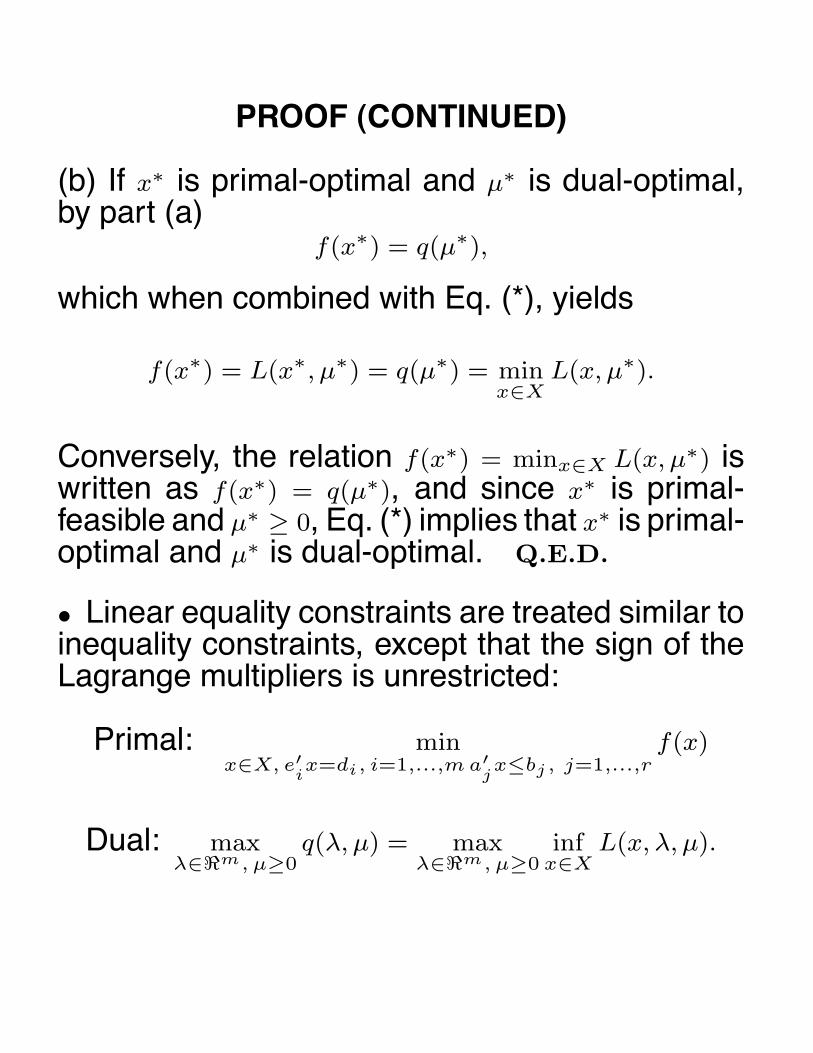
(b) If x∗ is primal-optimal and µ∗ is dual-optimal,by part (a)

f(x∗) = q(µ∗),

which when combined with Eq. (*), yields

f(x∗) = L(x∗, µ∗) = q(µ∗) = minx∈X

L(x, µ∗).

Conversely, the relation f(x∗) = minx∈X L(x, µ∗) iswritten as f(x∗) = q(µ∗), and since x∗ is primal-feasible and µ∗ ≥ 0, Eq. (*) implies that x∗ is primal-optimal and µ∗ is dual-optimal. Q.E.D.

• Linear equality constraints are treated similar toinequality constraints, except that the sign of theLagrange multipliers is unrestricted:

Primal: minx∈X, e′

ix=di, i=1,...,m a′

jx≤bj , j=1,...,r

f(x)

Dual: maxλ∈m, µ≥0

q(λ, µ) = maxλ∈m, µ≥0

infx∈X

L(x, λ, µ).

THE DUAL OF A LINEAR PROGRAM

• Consider the linear program

minimize c′x

subject to e′ix = di, i = 1, . . . , m, x ≥ 0

• Dual function

q(λ) = infx≥0

{n∑

j=1

(cj −

m∑i=1

λieij

)xj +

m∑i=1

λidi

}.

• If cj −∑m

i=1λieij ≥ 0 for all j, the infimum is

attained for x = 0, and q(λ) =∑m

i=1λidi. If cj −∑m

i=1λieij < 0 for some j, the expression in braces

can be arbitrarily small by taking xj suff. large, soq(λ) = −∞. Thus, the dual is

maximizem∑

i=1

λidi

subject tom∑

i=1

λieij ≤ cj , j = 1, . . . , n.

THE DUAL OF A QUADRATIC PROGRAM

• Consider the quadratic programminimize 1

2x′Qx + c′x

subject to Ax ≤ b,

where Q is a given n×n positive definite symmetricmatrix, A is a given r × n matrix, and b ∈ �r andc ∈ �n are given vectors.

• Dual function:

q(µ) = infx∈n

{12x′Qx + c′x + µ′(Ax − b)

}.

The infimum is attained for x = −Q−1(c+A′µ), and,after substitution and calculation,

q(µ) = − 12µ′AQ−1A′µ − µ′(b + AQ−1c) − 1

2 c′Q−1c.

• The dual problem, after a sign change, isminimize 1

2µ′Pµ + t′µ

subject to µ ≥ 0,

where P = AQ−1A′ and t = b + AQ−1c.


LECTURE 15: INTERIOR POINT METHODS

LECTURE OUTLINE

• Barrier and Interior Point Methods

• Linear Programs and the Logarithmic Barrier

• Path Following Using Newton’s Method

Inequality constrained problem

minimize f(x)

subject to x ∈ X, gj(x) ≤ 0, j = 1, . . . , r,

where f and gj are continuous and X is closed.We assume that the set

S ={

x ∈ X | gj(x) < 0, j = 1, . . . , r}

is nonempty and any feasible point is in the closureof S.

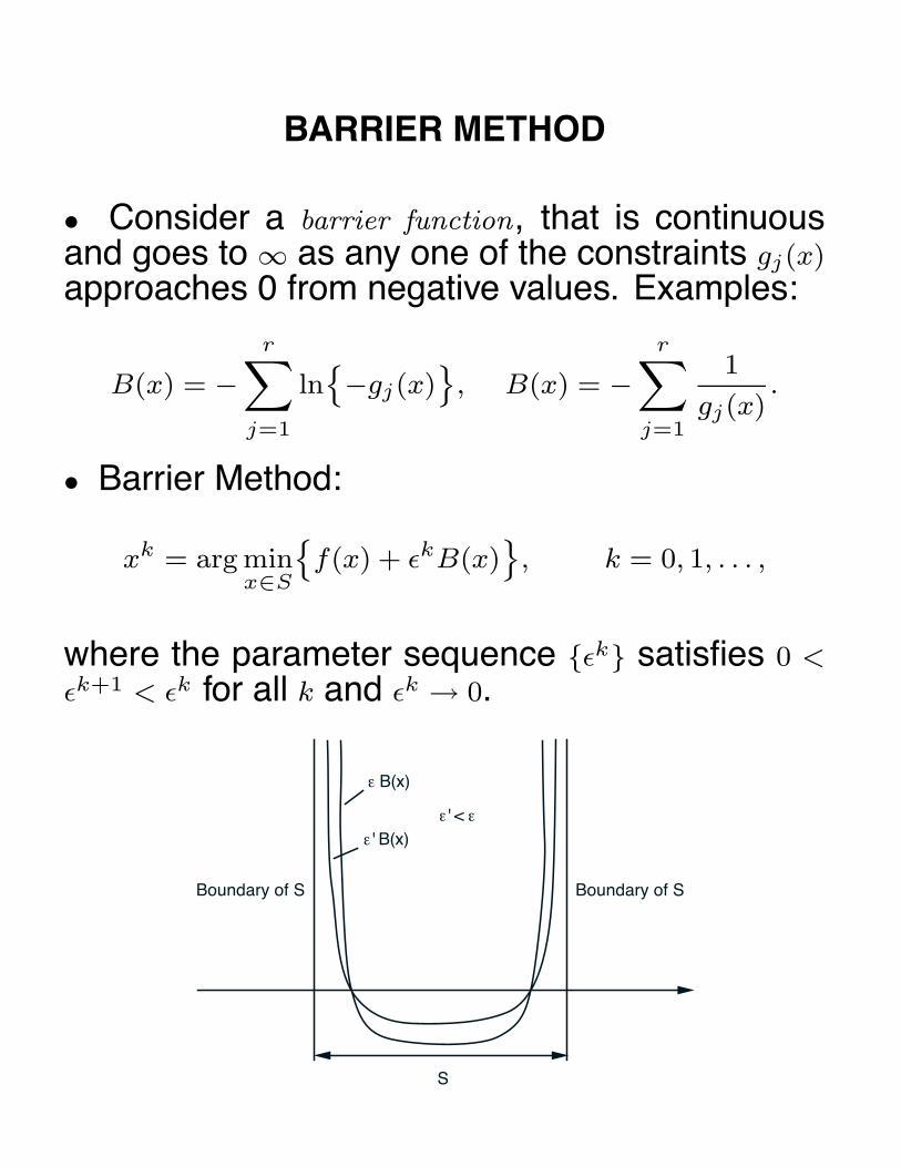
BARRIER METHOD

• Consider a barrier function, that is continuousand goes to ∞ as any one of the constraints gj(x)

approaches 0 from negative values. Examples:

B(x) = −r∑

j=1

ln{−gj(x)

}, B(x) = −

r∑j=1

1

gj(x).

• Barrier Method:

xk = arg minx∈S

{f(x) + εkB(x)

}, k = 0, 1, . . . ,

where the parameter sequence {εk} satisfies 0 <

εk+1 < εk for all k and εk → 0.

S

Boundary of S Boundary of S

ε B(x)

ε ' B(x)ε ' < ε

CONVERGENCE

Every limit point of a sequence {xk} generatedby a barrier method is a global minimum of theoriginal constrained problem

Proof: Let {x} be the limit of a subsequence {xk}k∈K .Since xk ∈ S and X is closed, x is feasible for theoriginal problem. If x is not a global minimum,there exists a feasible x∗ such that f(x∗) < f(x)

and therefore also an interior point x̃ ∈ S such thatf(x̃) < f(x). By the definition of xk, f(xk)+εkB(xk) ≤f(x̃) + εkB(x̃) for all k, so by taking limit

f(x) + lim infk→∞, k∈K

εkB(xk) ≤ f(x̃) < f(x)

Hence lim infk→∞, k∈K εkB(xk) < 0.If x ∈ S, we have limk→∞, k∈K εkB(xk) = 0,

while if x lies on the boundary of S, we have byassumption limk→∞, k∈K B(xk) = ∞. Thus

lim infk→∞

εkB(xk) ≥ 0,

– a contradiction.

LINEAR PROGRAMS/LOGARITHMIC BARRIER

• Apply logarithmic barrier to the linear programminimize c′x

subject to Ax = b, x ≥ 0,(LP)

The method finds for various ε > 0,

x(ε) = arg minx∈S

Fε(x) = arg minx∈S

{c′x − ε

n∑i=1

ln xi

},

where S ={

x | Ax = b, x > 0}. We assume that S isnonempty and bounded.

• As ε → 0, x(ε) follows the central path

Point x(ε) oncentral path

x∞

S

x* (ε = 0)

c

All central paths start at

the analytic center

x∞ = arg minx∈S

{−

n∑i=1

ln xi

},

and end at optimal solu-

tions of (LP).

PATH FOLLOWING W/ NEWTON’S METHOD

• Newton’s method for minimizing Fε:x̃ = x + α(x − x),

where x is the pure Newton iterate

x = arg minAz=b

{∇Fε(x)′(z − x) + 1

2 (z − x)′∇2Fε(x)(z − x)}

• By straightforward calculation

x = x − Xq(x, ε),

q(x, ε) =Xz

ε− e, e = (1 . . . 1)′, z = c − A′λ,

λ = (AX2A′)−1AX(Xc − εe

),

and X is the diagonal matrix with xi, i = 1, . . . , n

along the diagonal.

• View q(x, ε) as the Newton increment (x−x) trans-formed by X−1 that maps x into e.

• Consider ‖q(x, ε)‖ as a proximity measure of thecurrent point to the point x(ε) on the central path.

KEY RESULTS

• It is sufficient to minimize Fε approximately, upto where ‖q(x, ε)‖ < 1.

x∞

S

x*

Central Path

Set {x | ||q(x,ε0)|| < 1}

x(ε2)

x(ε1)

x(ε0)x0

x2

x1

If x > 0, Ax = b, and

‖q(x, ε)‖ < 1, then

c′x− minAy=b, y≥0

c′y ≤ ε(n+

√n).

• The “termination set”{

x | ‖q(x, ε)‖ < 1}

is partof the region of quadratic convergence of the pureform of Newton’s method. In particular, if ‖q(x, ε)‖ <

1, then the pure Newton iterate x = x − Xq(x, ε) isan interior point, that is, x ∈ S. Furthermore, wehave ‖q(x, ε)‖ < 1 and in fact

‖q(x, ε)‖ ≤ ‖q(x, ε)‖2.

SHORT STEP METHODS

S

x*

Central Path

Set {x | ||q(x,εk)|| < 1}

x∞

x(εk+1)

x(εk)xk

xk+1

Set {x | ||q(x,εk+1)|| < 1}

Following approximately the

central path by using a sin-

gle Newton step for each

εk. If εk is close to εk+1

and xk is close to the cen-

tral path, one expects that

xk+1 obtained from xk by

a single pure Newton step

will also be close to the

central path.

Proposition Let x > 0, Ax = b, and suppose thatfor some γ < 1 we have ‖q(x, ε)‖ ≤ γ. Then if ε =

(1 − δn−1/2)ε for some δ > 0,

‖q(x, ε)‖ ≤ γ2 + δ

1 − δn−1/2.

In particular, ifδ ≤ γ(1 − γ)(1 + γ)−1,

we have ‖q(x, ε)‖ ≤ γ.

• Can be used to establish nice complexity results;but ε must be reduced VERY slowly.

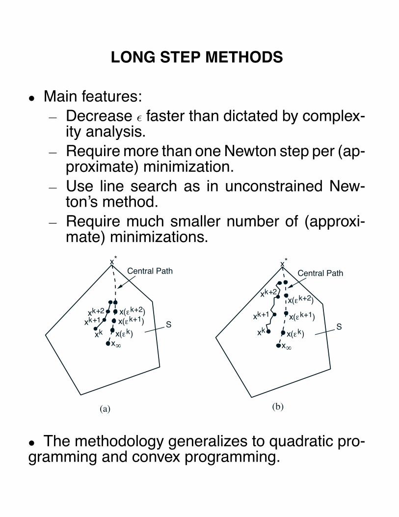
LONG STEP METHODS

• Main features:− Decrease ε faster than dictated by complex-

ity analysis.− Require more than one Newton step per (ap-

proximate) minimization.− Use line search as in unconstrained New-

ton’s method.− Require much smaller number of (approxi-

mate) minimizations.

S

x*

Central Path

x∞

x(εk+1)

x(εk)xk

xk+1 x(εk+2)xk+2

(a) (b)

S

x*

Central Path

x∞

x(εk+1)

x(εk)xk

xk+1

x(εk+2)xk+2

• The methodology generalizes to quadratic pro-gramming and convex programming.


LECTURE 16: PENALTY METHODS

LECTURE OUTLINE

• Quadratic Penalty Methods

• Introduction to Multiplier Methods

*******************************************

• Consider the equality constrained problem

minimize f(x)

subject to x ∈ X, h(x) = 0,

where f : �n → � and h : �n → �m are continuous,and X is closed.

• The quadratic penalty method:

xk = arg minx∈X

Lck (x, λk) ≡ f(x) + λk′h(x) +

ck

2‖h(x)‖2

where the {λk} is a bounded sequence and {ck}satisfies 0 < ck < ck+1 for all k and ck → ∞.

TWO CONVERGENCE MECHANISMS

• Taking λk close to a Lagrange multiplier vector− Assume X = �n and (x∗, λ∗) is a local min-

Lagrange multiplier pair satisfying the 2ndorder sufficiency conditions

− For c suff. large, x∗ is a strict local min ofLc(·, λ∗)

• Taking ck very large− For large c and any λ

Lc(·, λ) ≈{

f(x) if x ∈ X and h(x) = 0

∞ otherwise

• Example:minimize f(x) = 1

2 (x21 + x2

2)

subject to x1 = 1

Lc(x, λ) = 12 (x2

1 + x22) + λ(x1 − 1) +

c

2(x1 − 1)2

x1(λ, c) =c − λ

c + 1, x2(λ, c) = 0

EXAMPLE CONTINUED

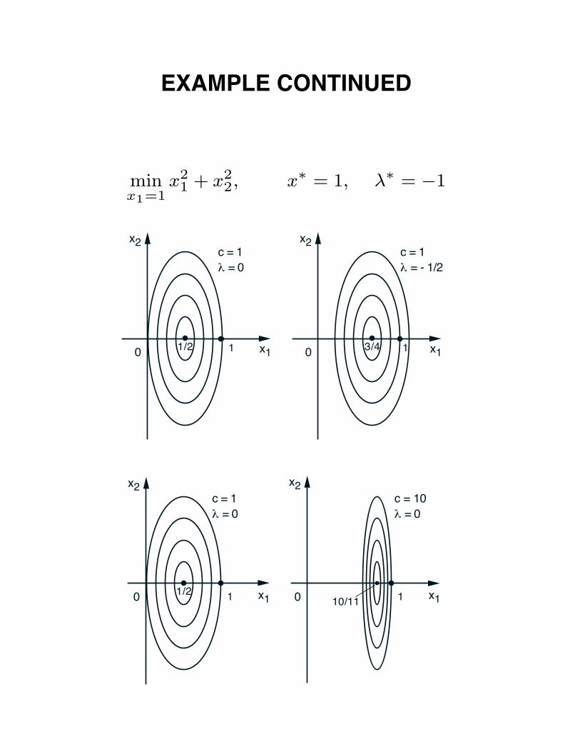
minx1=1

x21 + x2

2, x∗ = 1, λ∗ = −1

0 x13/4

x2

10 x11/2

x2

1

c = 1λ = 0

c = 1λ = - 1/2

0 x11/2

x2

1 0 x110/11

x2

1

c = 1λ = 0

c = 10λ = 0

GLOBAL CONVERGENCE

• Every limit point of {xk} is a global min.

Proof: The optimal value of the problem is f∗ =

infh(x)=0, x∈X Lck (x, λk). We have

Lck (xk, λk) ≤ Lck (x, λk), ∀ x ∈ X

so taking the inf of the RHS over x ∈ X, h(x) = 0

Lck (xk, λk) = f(xk) + λk′h(xk) +

ck

2‖h(xk)‖2 ≤ f∗.

Let (x̄, λ̄) be a limit point of {xk, λk}. Without lossof generality, assume that {xk, λk} → (x̄, λ̄). Takingthe limsup above

f(x̄) + λ̄′h(x̄) + lim supk→∞

ck

2‖h(xk)‖2 ≤ f∗. (*)

Since ‖h(xk)‖2 ≥ 0 and ck → ∞, it follows thath(xk) → 0 and h(x̄) = 0. Hence, x̄ is feasible, andsince from Eq. (*) we have f(x̄) ≤ f∗, x̄ is optimal.Q.E.D.

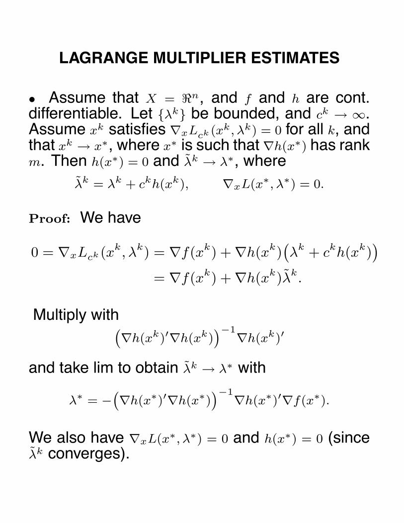
LAGRANGE MULTIPLIER ESTIMATES

• Assume that X = �n, and f and h are cont.differentiable. Let {λk} be bounded, and ck → ∞.Assume xk satisfies ∇xLck (xk, λk) = 0 for all k, andthat xk → x∗, where x∗ is such that ∇h(x∗) has rankm. Then h(x∗) = 0 and λ̃k → λ∗, where

λ̃k = λk + ckh(xk), ∇xL(x∗, λ∗) = 0.

Proof: We have

0 = ∇xLck (xk, λk) = ∇f(xk) + ∇h(xk)(λk + ckh(xk)

)= ∇f(xk) + ∇h(xk)λ̃k.

Multiply with(∇h(xk)′∇h(xk)

)−1∇h(xk)′

and take lim to obtain λ̃k → λ∗ with

λ∗ = −(∇h(x∗)′∇h(x∗)

)−1∇h(x∗)′∇f(x∗).

We also have ∇xL(x∗, λ∗) = 0 and h(x∗) = 0 (sinceλ̃k converges).

PRACTICAL BEHAVIOR

• Three possibilities:− The method breaks down because an xk with

∇xLck (xk, λk) ≈ 0 cannot be found.− A sequence {xk} with ∇xLck (xk, λk) ≈ 0 is ob-

tained, but it either has no limit points, or foreach of its limit points x∗ the matrix ∇h(x∗)

has rank < m.− A sequence {xk} with with ∇xLck (xk, λk) ≈ 0

is found and it has a limit point x∗ such that∇h(x∗) has rank m. Then, x∗ together with λ∗

[the corresp. limit point of{

λk +ckh(xk)}

] sat-isfies the first-order necessary conditions.

• Ill-conditioning: The condition number of theHessian ∇2

xxLck (xk, λk) tends to increase with ck.

• To overcome ill-conditioning:− Use Newton-like method (and double preci-

sion).− Use good starting points.− Increase ck at a moderate rate (if ck is in-

creased at a fast rate, {xk} converges faster,but the likelihood of ill-conditioning is greater).

INEQUALITY CONSTRAINTS

• Convert them to equality constraints by usingsquared slack variables that are eliminated later.

• Convert inequality constraint gj(x) ≤ 0 to equalityconstraint gj(x) + z2

j = 0.

• The penalty method solves problems of the form

minx,z

L̄c(x, z, λ, µ) = f(x)

+

r∑j=1

{µj

(gj(x) + z2

j

)+

c

2|gj(x) + z2

j |2}

,

for various values of µ and c.

• First minimize L̄c(x, z, λ, µ) with respect to z,

Lc(x, λ, µ) = minz

L̄c(x, z, λ, µ) = f(x)

+

r∑j=1

minzj

{µj

(gj(x) + z2

j

)+

c

2|gj(x) + z2

j |2}

and then minimize Lc(x, λ, µ) with respect to x.

MULTIPLIER METHODS

• Recall that if (x∗, λ∗) is a local min-Lagrangemultiplier pair satisfying the 2nd order sufficiencyconditions, then for c suff. large, x∗ is a strict localmin of Lc(·, λ∗).

• This suggests that for λk ≈ λ∗, xk ≈ x∗.

• Hence it is a good idea to use λk ≈ λ∗, such as

λk+1 = λ̃k = λk + ckh(xk)

This is the (1st order) method of multipliers.

• Key advantages to be shown:− Less ill-conditioning: It is not necessary that

ck → ∞ (only that ck exceeds some thresh-old).

− Faster convergence when λk is updated thanwhen λk is kept constant (whether ck → ∞ ornot).


LECTURE 17: AUGMENTED LAGRANGIAN METHODS

LECTURE OUTLINE

• Multiplier Methods

*******************************************

• Consider the equality constrained problemminimize f(x)

subject to h(x) = 0,

where f : �n → � and h : �n → �m are continuouslydifferentiable.

• The (1st order) multiplier method finds

xk = arg minx∈n

Lck (x, λk) ≡ f(x) + λk′h(x) +

ck

2‖h(x)‖2

and updates λk using

λk+1 = λk + ckh(xk)

CONVEX EXAMPLE

• Problem: minx1=1(1/2)(x21 + x2

2) with optimal so-lution x∗ = (1, 0) and Lagr. multiplier λ∗ = −1.

• We have

xk = arg minx∈n

Lck (x, λk) =

(ck − λk

ck + 1, 0

)

λk+1 = λk + ck

(ck − λk

ck + 1− 1

)

λk+1 − λ∗ =λk − λ∗

ck + 1

• We see that:− λk → λ∗ = −1 and xk → x∗ = (1, 0) for ev-

ery nondecreasing sequence {ck}. It is NOTnecessary to increase ck to ∞.

− The convergence rate becomes faster as ck

becomes larger; in fact{|λk−λ∗|

}converges

superlinearly if ck → ∞.

NONCONVEX EXAMPLE

• Problem: minx1=1(1/2)(−x21 + x2

2) with optimal so-lution x∗ = (1, 0) and Lagr. multiplier λ∗ = 1.

• We have

xk = arg minx∈n

Lck (x, λk) =

(ck − λk

ck − 1, 0

)

provided ck > 1 (otherwise the min does not exist)

λk+1 = λk + ck

(ck − λk

ck − 1− 1

)

λk+1 − λ∗ = −λk − λ∗

ck − 1

• We see that:− No need to increase ck to ∞ for convergence;

doing so results in faster convergence rate.− To obtain convergence, ck must eventually

exceed the threshold 2.

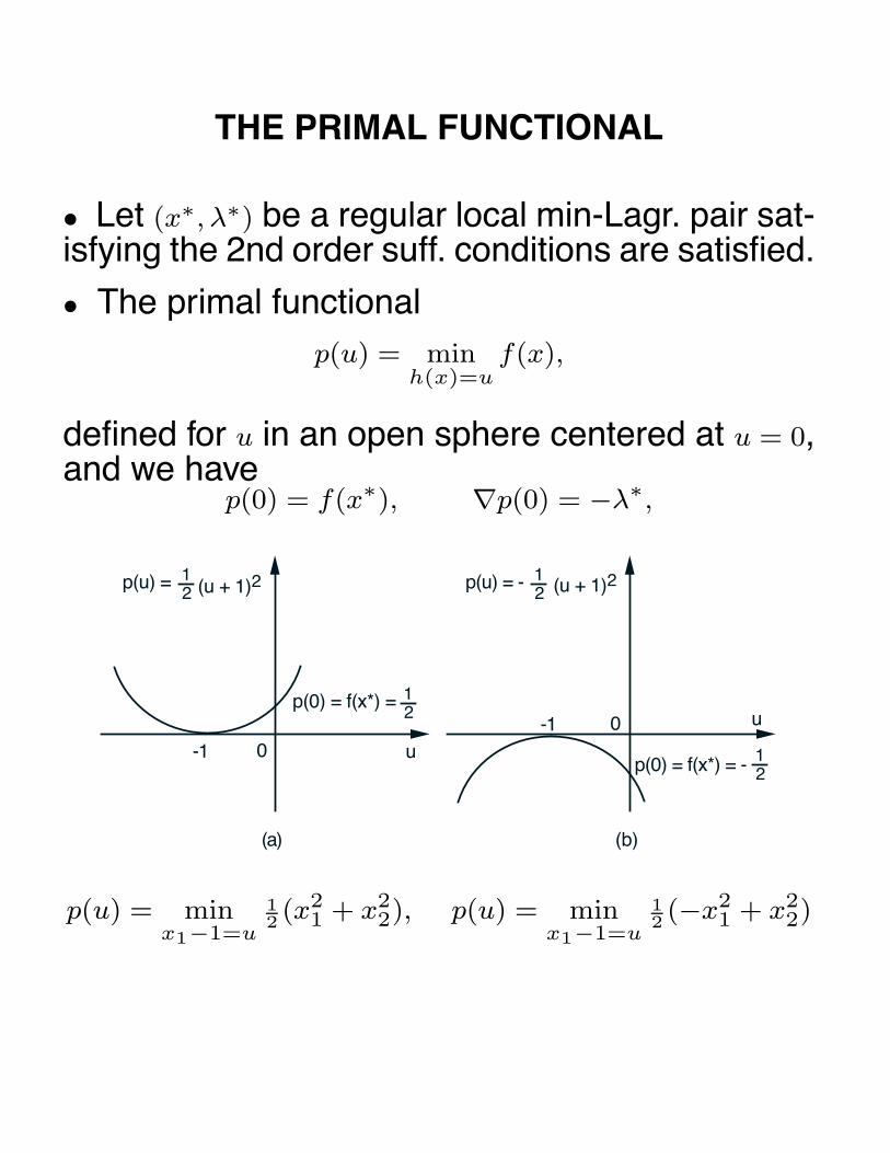
THE PRIMAL FUNCTIONAL

• Let (x∗, λ∗) be a regular local min-Lagr. pair sat-isfying the 2nd order suff. conditions are satisfied.

• The primal functionalp(u) = min

h(x)=uf(x),

defined for u in an open sphere centered at u = 0,and we have

p(0) = f(x∗), ∇p(0) = −λ∗,

0 u

(u + 1)212

p(u) =

p(0) = f(x*) = 12

-1 0 u

(u + 1)212

p(u) = -

p(0) = f(x*) = - 12

-1

(a) (b)

p(u) = minx1−1=u

12 (x2

1 + x22), p(u) = min

x1−1=u

12 (−x2

1 + x22)

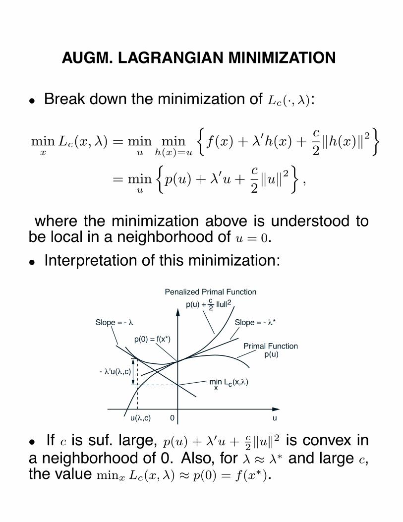
AUGM. LAGRANGIAN MINIMIZATION

• Break down the minimization of Lc(·, λ):

minx

Lc(x, λ) = minu

minh(x)=u

{f(x) + λ′h(x) +

c

2‖h(x)‖2

}= min

u

{p(u) + λ′u +

c

2‖u‖2

},

where the minimization above is understood tobe local in a neighborhood of u = 0.

• Interpretation of this minimization:

p(0) = f(x*)

p(u)

Slope = - λ*

min Lc(x,λ)x

Slope = - λ

0 uu(λ,c)

- λ'u(λ,c)

Primal Function

||u||2c2p(u) +

Penalized Primal Function

• If c is suf. large, p(u) + λ′u + c2‖u‖2 is convex in

a neighborhood of 0. Also, for λ ≈ λ∗ and large c,the value minx Lc(x, λ) ≈ p(0) = f(x∗).

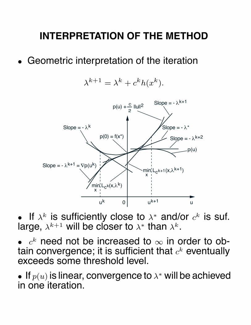
INTERPRETATION OF THE METHOD

• Geometric interpretation of the iteration

λk+1 = λk + ckh(xk).

p(0) = f(x*)

p(u)

Slope = - λ*

min Lck(x,λk)x

Slope = - λk

Slope = - λk+1 = ∇p(uk)

Slope = - λk+1

Slope = - λk+2

0 uuk uk+1

min Lck+1(x,λk+1)x

||u||2c

2p(u) +

• If λk is sufficiently close to λ∗ and/or ck is suf.large, λk+1 will be closer to λ∗ than λk.

• ck need not be increased to ∞ in order to ob-tain convergence; it is sufficient that ck eventuallyexceeds some threshold level.

• If p(u) is linear, convergence to λ∗ will be achievedin one iteration.

COMPUTATIONAL ASPECTS

• Key issue is how to select {ck}.− ck should eventually become larger than the

“threshold” of the given problem.− c0 should not be so large as to cause ill-

conditioning at the 1st minimization.− ck should not be increased so fast that too

much ill-conditioning is forced upon the un-constrained minimization too early.

− ck should not be increased so slowly thatthe multiplier iteration has poor convergencerate.

• A good practical scheme is to choose a mod-erate value c0, and use ck+1 = βck, where β is ascalar with β > 1 (typically β ∈ [5, 10] if a Newton-like method is used).

• In practice the minimization of Lck (x, λk) is typ-ically inexact (usually exact asymptotically). Insome variants of the method, only one Newtonstep per minimization is used (with safeguards).

DUALITY FRAMEWORK


minimize f(x) +c

2‖h(x)‖2

subject to ‖x − x∗‖ < ε, h(x) = 0,

where ε is small enough for a local analysis tohold based on the implicit function theorem, and c

is large enough for the minimum to exist.

• Consider the dual function and its gradient

qc(λ) = min‖x−x∗‖<ε

Lc(x, λ) = Lc

(x(λ, c), λ

)

∇qc(λ) = ∇λx(λ, c)∇xLc

(x(λ, c), λ

)+ h

(x(λ, c)

)= h

(x(λ, c)

).

We have ∇qc(λ∗) = h(x∗) = 0 and ∇2qc(λ∗) < 0.

• The multiplier method is a steepest ascent iter-ation for maximizing qck

λk+1 = λk + ck∇qck (λk),


LECTURE 18: DUALITY THEORY

LECTURE OUTLINE

• Geometrical Framework for Duality

• Geometric Multipliers

• The Dual Problem

• Properties of the Dual Function


minimize f(x)


• We assume that the problem is feasible and thecost is bounded from below:

−∞ < f∗ = infx∈X

gj(x)≤0, j=1,...,r

f(x) < ∞

MIN COMMON POINT/MAX CROSSING POINT

• Let M be a subset of �n:

• Min Common Point Problem: Among all points thatare common to both M and the nth axis,find theone whose nth component is minimum.

• Max Crossing Point Problem: Among all hyper-planes that intersect the nth axis and support theset M from “below”, find the hyperplane for whichpoint of intercept with the nth axis is maximum.

0

Min Common Point w*

Max Crossing Point q*

M

0

M

Max Crossing Point q*

Min Common Point w*w w

uu

• Note: We will see that the min common/maxcrossing framework applies to the problem of thepreceding slide, i.e., minx∈X, g(x)≤0f(x), with thechoice

M ={

(z, f(x)) | g(x) ≤ z, x ∈ X}

GEOMETRICAL DEFINITION OF A MULTIPLIER

• A vector µ∗ = (µ∗1, . . . , µ∗

r) is said to be a geometric

multiplier for the primal problem if

µ∗j ≥ 0, j = 1, . . . , r,

andf∗ = inf

x∈XL(x, µ∗).

0

(a)

(0,f*)

(µ*,1)

w

z

H = {(z,w) | f* = w + Σ j µjzj}*

0

(b)

(0,f*)(µ*,1)

Set of pairs (z,w) corresponding to x that minimize L(x,µ*) over X

S = {(g(x),f(x)) | x ∈ X} S = {(g(x),f(x)) | x ∈ X}

z

w

• Note that the definition differs from the one givenin Chapter 3 ... but if X = �n, f and gj are convexand differentiable, and x∗ is an optimal solution,the Lagrange multipliers corresponding to x∗, asper the definition of Chapter 3, coincide with thegeometric multipliers as per the above definition.

EXAMPLES: A G-MULTIPLIER EXISTS

0(-1,0)

(µ*,1) min f(x) = (1/2) (x12 + x2

2)s.t. g(x) = x1 - 1 ≤ 0

x ∈ X = R2

(b)

0

(0,-1)

(µ*,1)

(0,1) min f(x) = x1 - x2s.t. g(x) = x1 + x2 - 1 ≤ 0

x ∈ X = {(x1,x2) | x1 ≥ 0, x2 ≥ 0}

(a)

(-1,0)

0

(µ*,1)

min f(x) = |x1| + x2s.t. g(x) = x1 ≤ 0

x ∈ X = {(x1,x2) | x2 ≥ 0}

(c)

(µ*,1)

(µ*,1)

S = {(g(x),f(x)) | x ∈ X}

S = {(g(x),f(x)) | x ∈ X}

S = {(g(x),f(x)) | x ∈ X}

EXAMPLES: A G-MULTIPLIER DOESN’T EXIST

min f(x) = x

s.t. g(x) = x2 ≤ 0 x ∈ X = R

(a)(0,f*) = (0,0)

(-1/2,0)

S = {(g(x),f(x)) | x ∈ X}min f(x) = - x

s.t. g(x) = x - 1/2 ≤ 0 x ∈ X = {0,1}

(b)

(0,f*) = (0,0)

(1/2,-1)

S = {(g(x),f(x)) | x ∈ X}

• Proposition: Let µ∗ be a geometric multiplier.Then x∗ is a global minimum of the primal problemif and only if x∗ is feasible and

x∗ = arg minx∈X

L(x, µ∗), µ∗j gj(x

∗) = 0, j = 1, . . . , r

THE DUAL FUNCTION AND THE DUAL PROBLEM

• The dual problem is

maximize q(µ)


where q is the dual function

q(µ) = infx∈X

L(x, µ), ∀ µ ∈ �r.

• Question: How does the optimal dual value q∗ =

supµ≥0 q(µ) relate to f∗?

(µ,1)

H = {(z,w) | w + µ'z = b}

OptimalDual Value

x ∈ Xq(µ) = inf L(x,µ)

Support pointscorrespond to minimizersof L(x,µ) over X

S = {(g(x),f(x)) | x ∈ X}

WEAK DUALITY

• The domain of q is

Dq ={

µ | q(µ) > −∞}

.

• Proposition: The domain Dq is a convex set andq is concave over Dq.

• Proposition: (Weak Duality Theorem) We have

q∗ ≤ f∗.

Proof: For all µ ≥ 0, and x ∈ X with g(x) ≤ 0, wehave

q(µ) = infz∈X

L(z, µ) ≤ f(x) +

r∑j=1

µjgj(x) ≤ f(x),

soq∗ = sup

µ≥0

q(µ) ≤ infx∈X, g(x)≤0

f(x) = f∗.

DUAL OPTIMAL SOLUTIONS AND G-MULTIPLIERS

• Proposition: (a) If q∗ = f∗, the set of geometricmultipliers is equal to the set of optimal dual solu-tions. (b) If q∗ < f∗, the set of geometric multipliersis empty.

Proof: By definition, a vector µ∗ ≥ 0 is a geometricmultiplier if and only if f∗ = q(µ∗) ≤ q∗, which by theweak duality theorem, holds if and only if there isno duality gap and µ∗ is a dual optimal solution.Q.E.D.

(a)

f* = 0

µ

q(µ)

1

(b)

µ

q(µ)

f* = 0

- 1

min f(x) = x

s.t. g(x) = x2 ≤ 0 x ∈ X = R

min f(x) = - x

s.t. g(x) = x - 1/2 ≤ 0 x ∈ X = {0,1}

q(µ) = min {x + µx2} ={- 1/(4 µ) if µ > 0

- ∞ if µ ≤ 0

- 1/2

x ∈ R

q(µ) = min { - x + µ(x - 1/2)} = min{ - µ/2, µ/2 −1} x ∈ {0,1}


LECTURE 19: DUALITY THEOREMS

LECTURE OUTLINE

• Duality and G-multipliers (continued)


minimize f(x)


assuming −∞ < f∗ < ∞.

• µ∗ is a geometric multiplier if µ∗ ≥ 0 and f∗ =

infx∈X L(x, µ∗).

• The dual problem is

maximize q(µ)


where q is the dual function q(µ) = infx∈X L(x, µ).

DUAL OPTIMALITY

(µ,1)

H = {(z,w) | w + µ'z = b}

OptimalDual Value

x ∈ Xq(µ) = inf L(x,µ)

Support pointscorrespond to minimizersof L(x,µ) over X

S = {(g(x),f(x)) | x ∈ X}

• Weak Duality Theorem: q∗ ≤ f∗.

• Geometric Multipliers and Dual Optimal Solu-tions:

(a) If there is no duality gap, the set of geometricmultipliers is equal to the set of optimal dualsolutions.

(b) If there is a duality gap, the set of geometricmultipliers is empty.

DUALITY PROPERTIES

• Optimality Conditions: (x∗, µ∗) is an optimal solution-geometric multiplier pair if and only if

x∗ ∈ X, g(x∗) ≤ 0, (Primal Feasibility),µ∗ ≥ 0, (Dual Feasibility),

x∗ = arg minx∈X

L(x, µ∗), (Lagrangian Optimality),

µ∗j gj(x

∗) = 0, j = 1, . . . , r, (Compl. Slackness).

• Saddle Point Theorem: (x∗, µ∗) is an optimalsolution-geometric multiplier pair if and only if x∗ ∈X, µ∗ ≥ 0, and (x∗, µ∗) is a saddle point of the La-grangian, in the sense that

L(x∗, µ) ≤ L(x∗, µ∗) ≤ L(x, µ∗), ∀ x ∈ X, µ ≥ 0.

INFEASIBLE AND UNBOUNDED PROBLEMS

0

min f(x) = 1/x

s.t. g(x) = x ≤ 0

x ∈ X = {x | x > 0}

(a)f* = ∞, q* = ∞

0

S = {(x2,x) | x > 0}

min f(x) = x

s.t. g(x) = x2 ≤ 0

x ∈ X = {x | x > 0}

(b)

f* = ∞, q* = 0

0

S = {(g(x),f(x)) | x ∈ X} = {(z,w) | z > 0}

min f(x) = x1 + x2s.t. g(x) = x1 ≤ 0

x ∈ X = {(x1,x2) | x1 > 0}

(c)f* = ∞, q* = −∞

z

w

w

w

z

z

S = {(g(x),f(x)) | x ∈ X}

EXTENSIONS AND APPLICATIONS

• Equality constraints hi(x) = 0, i = 1, . . . , m, canbe converted into the two inequality constraints

hi(x) ≤ 0, −hi(x) ≤ 0.

• Separable problems:

minimize

m∑i=1

fi(xi)

subject to

m∑i=1

gij(xi) ≤ 0, j = 1, . . . , r,

xi ∈ Xi, i = 1, . . . , m.

• Separable problem with a single constraint:

minimizen∑

i=1

fi(xi)

subject ton∑

i=1

xi ≥ A, αi ≤ xi ≤ βi, ∀ i.

DUALITY THEOREM I FOR CONVEX PROBLEMS

• Strong Duality Theorem - Linear Constraints:Assume that the problem

minimize f(x)

subject to x ∈ X, a′ix − bi = 0, i = 1, . . . , m,

e′jx − dj ≤ 0, j = 1, . . . , r,

has finite optimal value f∗. Let also f be convexover �n and let X be polyhedral. Then there existsat least one geometric multiplier and there is noduality gap.

• Proof Issues

• Application to Linear Programming

COUNTEREXAMPLE

• A Convex Problem with a Duality Gap: Considerthe two-dimensional problem

minimize f(x)

subject to x1 ≤ 0, x ∈ X = {x | x ≥ 0},

wheref(x) = e−

√x1x2 , ∀ x ∈ X,

and f(x) is arbitrarily defined for x /∈ X.

• f is convex over X (its Hessian is positive definitein the interior of X), and f∗ = 1.

• Also, for all µ ≥ 0 we have

q(µ) = infx≥0

{e−

√x1x2 + µx1

}= 0,

since the expression in braces is nonnegative forx ≥ 0 and can approach zero by taking x1 → 0 andx1x2 → ∞. It follows that q∗ = 0.

DUALITY THEOREM II FOR CONVEX PROBLEMS


minimize f(x)

subject to x ∈ X, gj(x) ≤ 0, j = 1, . . . , r.

• Assume that X is convex and the functionsf : �n �→ �, gj : �n �→ � are convex over X. Fur-thermore, the optimal value f∗ is finite and thereexists a vector x̄ ∈ X such that

gj(x̄) < 0, ∀ j = 1, . . . , r.

• Strong Duality Theorem: There exists at leastone geometric multiplier and there is no dualitygap.

• Extension to linear equality constraints.


LECTURE 20: STRONG DUALITY

LECTURE OUTLINE

• Strong Duality Theorem

• Linear Equality Constraints

• Fenchel Duality

********************************


minimize f(x)



• µ∗ is a geometric multiplier if µ∗ ≥ 0 and f∗ =

infx∈X L(x, µ∗).

• Dual problem: Maximize q(µ) = infx∈X L(x, µ)

subject to µ ≥ 0.

DUALITY THEOREM FOR INEQUALITIES

• Assume that X is convex and the functionsf : �n �→ �, gj : �n �→ � are convex over X. Fur-thermore, the optimal value f∗ is finite and thereexists a vector x̄ ∈ X such that

gj(x̄) < 0, ∀ j = 1, . . . , r.

• Strong Duality Theorem: There exists at leastone geometric multiplier and there is no dualitygap.

(0,f*)

(µ,1)

w

z

A = {(z,w) | there is an x in X such that g(x) ≤ z, f(x) ≤ w}

(g(x),f(x)) S = {(g(x),f(x)) | x ∈ X}

PROOF OUTLINE

• Show that A is convex. [Consider vectors (z, w) ∈A and (z̃, w̃) ∈ A, and show that their convex com-binations lie in A.]

• Observe that (0, f∗) is not an interior point of A.

• Hence, there is hyperplane passing through(0, f∗) and containing A in one of the two corre-sponding halfspaces; i.e., a (µ, β) �= (0, 0) with

βf∗ ≤ βw + µ′z, ∀ (z, w) ∈ A.

This implies that β ≥ 0, and µj ≥ 0 for all j.

• Prove that the hyperplane is nonvertical, i.e.,β > 0.

• Normalize (β = 1), take the infimum over x ∈ X,and use the fact µ ≥ 0, to obtain

f∗ ≤ infx∈X

{f(x) + µ′g(x)

}= q(µ) ≤ sup

µ≥0

q(µ) = q∗.

Using the weak duality theorem, µ is a geometricmultiplier and there is no duality gap.

LINEAR EQUALITY CONSTRAINTS

• Suppose we have the additional constraints

e′ix − di = 0, i = 1, . . . , m

• We need the notion of the affine hull of a convexset X [denoted aff(X)]. This is the intersection ofall hyperplanes containing X.

• The relative interior of X, denoted ri(X), is the setof all x ∈ X s.t. there exists ε > 0 with{

z | ‖z − x‖ < ε, z ∈ aff(X)}

⊂ X,

that is, ri(X) is the interior of X relative to aff(X).

• Every nonempty convex set has a nonemptyrelative interior.

DUALITY THEOREM FOR EQUALITIES

• Assumptions:− The set X is convex and the functions f , gj

are convex over X.− The optimal value f∗ is finite and there exists

a vector x̄ ∈ ri(X) such that

gj(x̄) < 0, j = 1, . . . , r,

e′ix̄ − di = 0, i = 1, . . . , m.

• Under the preceding assumptions there existsat least one geometric multiplier and there is noduality gap.

COUNTEREXAMPLE

• Consider

minimize f(x) = x1

subject to x2 = 0, x ∈ X ={

(x1, x2) | x21 ≤ x2

}.

• The optimal solution is x∗ = (0, 0) and f∗ = 0.

• The dual function is given by

q(λ) = infx21≤x2

{x1 + λx2} =

{− 1

4λ, if λ > 0,

−∞, if λ ≤ 0.

• No dual optimal solution and therefore there isno geometric multiplier. (Even though there is noduality gap.)

• Assumptions are violated (the feasible set andthe relative interior of X have no common point).

FENCHEL DUALITY FRAMEWORK


minimize f1(x) − f2(x)

subject to x ∈ X1 ∩ X2,

where f1 and f2 are real-valued functions on �n,and X1 and X2 are subsets of �n.

• Assume that −∞ < f∗ < ∞.

• Convert problem to

minimize f1(y) − f2(z)

subject to z = y, y ∈ X1, z ∈ X2,

and dualize the constraint z = y.

q(λ) = infy∈X1, z∈X2

{f1(y) − f2(z) + (z − y)′λ

}= inf

z∈X2

{z′λ − f2(z)

}− sup

y∈X1

{y′λ − f1(y)

}= g2(λ) − g1(λ)

DUALITY THEOREM

0 x 0 xX1

f1(x)

(λ,-1)

(λ,-1)

Slope = λ

inf {f1(x) - x'λ} = - g1(λ)x ∈ X1

sup {f2(x) - x'λ} = - g2(λ)x ∈ X2

f2(x)

X2

Slope = λ

• Assume that− X1 and X2 are convex− f1 and f2 are convex and concave over X1

and X2, respectively− The relative interiors of X1 and X2 intersect

• The duality theorem for equalities applies andshows that

f∗ = maxλ∈n

{g2(λ) − g1(λ)

}and that the maximum above is attained.


• There is no duality gap, while simultaneously,(x∗, λ∗) is an optimal primal and dual solution pair,if and only if

x∗ ∈ X1 ∩ X2, (primal feasibility),

λ∗ ∈ Λ1 ∩ Λ2, (dual feasibility),

x∗ = arg maxx∈X1

{x′λ∗ − f1(x)

}= arg min

x∈X2

{x′λ∗ − f2(x)

}, (Lagr. optimality).

0 x

f1(x)

Slope = λg2(λ) - g1(λ)

x*

f2(x)

Slope = λ*

g2(λ*) - g1(λ*)

(- λ*,1)

(- λ,1)


LECTURE 21: DISCRETE OPTIMIZATION

LECTURE OUTLINE

• Discrete Constraints and Integer Programming

• Examples of Discrete Optimization Problems

• Constraint Relaxation and Rounding

• Branch-and-Bound

• Lagrangian Relaxation

********************************

• Consider

minimize f(x)


where X is a finite set.

• Example: 0-1 Integer programming:

X ={

(x1, . . . , xn) | xi = 0 or 1, i = 1, . . . , n}

.

EXAMPLES OF DISCRETE PROBLEMS

• Given a directed graph with set of nodes N andset of arcs (i, j) ∈ A, the (integer constrained) min-imum cost network flow problem is

minimize∑

(i,j)∈A

aijxij

subject to the constraints∑{j|(i,j)∈A}

xij −∑

{j|(j,i)∈A}

xji = si, ∀ i ∈ N ,

bij ≤ xij ≤ cij , ∀ (i, j) ∈ A, xij : integer,

where aij , bij , cij , and si are given scalars.

• Think of:− Nodes i with si > 0 and si < 0 as production

and consumption points, respectively.− si supply or demand of node i.− Arcs (i, j) as transportation links with flow ca-

pacity cij and cost per unit flow aij

− Problem is to accomplish a minimum costtransfer from the supply to the demand points.

• Important special cases: Shortest path, max-flow, transportation, assignment problems.

UNIMODULARITY PROPERTY

• The minimum cost flow problem has an inter-esting property: If the si and cij are integer, theoptimal solutions of the integer-constrained prob-lem also solve the relaxed problem, obtained whenthe integer constraints are neglected.

• Great practical significance, since the relaxedproblem can be solved using efficient linear (notinteger) programming algorithms.

• This is special case of unimodularity:− A square matrix A with integer components

is unimodular if its determinant is 0, 1, or -1.− If A is invertible and unimodular, by Kramer’s

rule, the inverse matrix A−1 has integer com-ponents. Hence, the solution x of the systemAx = b is integer for every integer vector b.

− A rectangular matrix with integer componentsis called totally unimodular if each of its squaresubmatrices is unimodular.

• A polyhedron {x | Ex = d, b ≤ x ≤ c} has integerextreme points if E is totally unimodular and b, c,and d have integer components.

• The matrix E corresponding to the minimum costflow problem is totally unimodular.

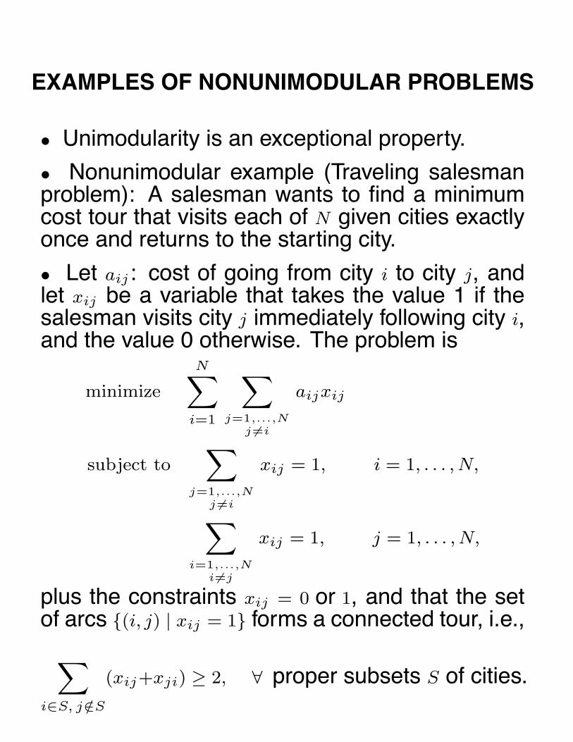
EXAMPLES OF NONUNIMODULAR PROBLEMS

• Unimodularity is an exceptional property.

• Nonunimodular example (Traveling salesmanproblem): A salesman wants to find a minimumcost tour that visits each of N given cities exactlyonce and returns to the starting city.

• Let aij : cost of going from city i to city j, andlet xij be a variable that takes the value 1 if thesalesman visits city j immediately following city i,and the value 0 otherwise. The problem is

minimize

N∑i=1

∑j=1,...,N

j �=i

aijxij

subject to∑

j=1,...,Nj �=i

xij = 1, i = 1, . . . , N,

∑i=1,...,N

i�=j

xij = 1, j = 1, . . . , N,

plus the constraints xij = 0 or 1, and that the setof arcs {(i, j) | xij = 1} forms a connected tour, i.e.,

∑i∈S, j /∈S

(xij+xji) ≥ 2, ∀ proper subsets S of cities.

APPROACHES TO INTEGER PROGRAMMING

• Enumeration of the finite set of all feasible (in-teger) solutions, and comparison to obtain an op-timal solution (this is rarely practical).

• Constraint relaxation and heuristic rounding.− Neglect the integer constraints− Solve the problem using linear/nonlinear pro-

gramming methods− If a noninteger solution is obtained, round it

to integer using a heuristic− Sometimes, with favorable structure, clever

problem formulation, and good heuristics,this works remarkably well

• Implicit enumeration (or branch-and-bound):− Combines the preceding two approaches− It uses constraint relaxation and solution of

noninteger problems to obtain certain lowerbounds that are used to discard large por-tions of the feasible set.

− In principle it can find an optimal (integer)solution, but this may require unacceptablelong time.

− In practice, usually it is terminated with aheuristically obtained integer solution, oftenderived by rounding a noninteger solution.

PRINCIPLE OF BRANCH-AND-BOUND

• Bounding Principle: Consider minimizing f(x)

over a finite set x ∈ X. Let Y1 and Y2 be two subsetsof X, and suppose that we have bounds

f1≤ min

x∈Y1f(x), f2 ≥ min

x∈Y2f(x).

Then, if f2 ≤ f1, the solutions in Y1 may be disre-

garded since their cost cannot be smaller than thecost of the best solution in Y2.

• The branch-and-bound method uses suitableupper and lower bounds, and the bounding prin-ciple to eliminate substantial portions of X.

• It uses a tree, with nodes that correspond tosubsets of X, usually obtained by binary partition.

X = {1,2,3,4,5}

{4}

Y = {1,2,3} {4,5}

{4} {5}

{1}

Y1 = {1,2} Y2 = {3}

Lower Bound fY_ _Feasible Solution x ∈ Y

{2}

BRANCH-AND-BOUND ALGORITHM

• The algorithm maintains a node list called OPEN,and a scalar called UPPER, which is equal to theminimal cost over feasible solutions found so far.Initially, OPEN= {X}, and UPPER= ∞ or to thecost f(x) of some feasible solution x ∈ X.

• Step 1: Remove a node Y from OPEN. Foreach child Yj of Y , do the following: Find the lowerbound f

Yjand a feasible solution x ∈ Yj . If

fYj

< UPPER,

place Yj in OPEN. If in additionf(x) < UPPER,

set UPPER = f(x) and mark x as the best solutionfound so far.

Step 2: (Termination Test) If OPEN is nonempty,go to step 1. Otherwise, terminate; the best solu-tion found so far is optimal.

• Termination with a global minimum is guaran-teed, but the number of nodes to be examined maybe huge. In practice, the algorithm is terminatedwhen an ε-optimal solution is obtained.

• Tight lower bounds fYj

are important for quick

termination.

LAGRANGIAN RELAXATION

• One method to obtain lower bounds in the branch-and-bound method is by constraint relaxation (e.g.,replace xi ∈ {0, 1} by 0 ≤ xi ≤ 1)

• Another method, called Lagrangian relaxation, isbased on weak duality. If the subproblem of anode of the branch-and-bound tree has the form

minimize f(x)

subject to gj(x) ≤ 0, j = 1, . . . , r,

x ∈ X,

use as lower bound the optimal dual valueq∗ = max

µ≥0q(µ),

where

q(µ) = minx∈X

{f(x) +

r∑j=1

µjgj(x)

}.

• Essential for applying Lagrangian relaxation isthat the dual problem is easy to solve (e.g., thedual is a simple linear program, or it involves use-ful structure, such as separability).


LECTURE 22: DUAL COMPUTATIONAL METHODS

LECTURE OUTLINE

• Dual Methods

• Nondifferentiable Optimization

********************************

• Consider the primal problem

minimize f(x)



• Dual problem: Maximize

q(µ) = infx∈X

L(x, µ) = infx∈X

{f(x) + µ′g(x)}

subject to µ ≥ 0.

PROS AND CONS FOR SOLVING THE DUAL

ADVANTAGES:

• The dual is concave.

• The dual may have smaller dimension and/orsimpler constraints.

• If there is no duality gap and the dual is solvedexactly for a geometric multiplier µ∗, all optimalprimal solutions can be obtained by minimizingthe Lagrangian L(x, µ∗) over x ∈ X.

• Even if there is a duality gap, q(µ) is a lowerbound to the optimal primal value for every µ ≥ 0.

DISADVANTAGES:

• Evaluating q(µ) requires minimization of L(x, µ)

over x ∈ X.

• The dual function is often nondifferentiable.

• Even if we find an optimal dual solution µ∗, it maybe difficult to obtain a primal optimal solution.

STRUCTURE

• Separability: Classical duality structure (La-grangian relaxation).

• Partitioning: The problem

minimize F (x) + G(y)

subject to Ax + By = c, x ∈ X, y ∈ Y

can be written as

minimize F (x) + infBy=c−Ax, y∈Y

G(y)

subject to x ∈ X.

With no duality gap, this problem is written asminimize F (x) + Q(Ax)

subject to x ∈ X,

whereQ(Ax) = max

λq(λ, Ax)

q(λ, Ax) = infy∈Y

{G(y) + λ′(Ax + By − c)

}

SUBGRADIENTS

• A vector d is said to be a subgradient at x of aconvex function f : �n �→ � if

f(z) ≥ f(x) + d′(z − x), ∀ z ∈ �n.

The set of subgradients at x is called the subdiffer-

ential and is denoted by ∂f(x).

z

(x, f(x))

f(z)

(-d, 1)

• If f is concave, d is said to be a subgradient at x if

f(z) ≤ f(x) + d′(z − x), ∀ z ∈ �n.

• Danskin’s Theorem: Consider the function f(x) =

maxz∈Z φ(x, z), where φ : �n+m �→ � is continuous,Z is compact, and φ(·, z) is convex for each z ∈ Z.Then f is convex and

∂f(x) = Convex Hull{

∂xφ(x, z) | z : attains the max}

DUAL DERIVATIVES

• Let

xµ = arg minx∈X

L(x, µ) = arg minx∈X

{f(x) + µ′g(x)

}.

Then for all µ̃ ∈ �r,

q(µ̃) = infx∈X

{f(x) + µ̃′g(x)

}≤ f(xµ) + µ̃′g(xµ)

= f(xµ) + µ′g(xµ) + (µ̃ − µ)′g(xµ)

= q(µ) + (µ̃ − µ)′g(xµ).

• Thus g(xµ) is a subgradient of q at µ.

• Proposition: Let X be compact, and let f and g

be continuous over X. Assume also that for everyµ, L(x, µ) is minimized over x ∈ X at a unique pointxµ. Then, q is everywhere continuously differen-tiable and

∇q(µ) = g(xµ), ∀ µ ∈ �r.

NONDIFFERENTIABLE DUAL

• If there exists a duality gap, the dual function isnondifferentiable at every dual optimal solution.

• Important nondifferentiable case: When q ispolyhedral, that is,

q(µ) = mini∈I

{a′

iµ + bi

},

where I is a finite index set, and ai ∈ �r and bi

are given (arises when X is a discrete set, as ininteger programming).

• Proposition: Let q be polyhedral as above, andlet Iµ be the set of indices attaining the minimum

Iµ ={

i ∈ I | a′iµ + bi = q(µ)

}.

The set of all subgradients of q at µ is

∂q(µ) =

⎧⎨⎩g

∣∣∣ g =∑i∈Iµ

ξiai, ξi ≥ 0,∑i∈Iµ

ξi = 1

⎫⎬⎭ .

NONDIFFERENTIABLE OPTIMIZATION

• Consider maximization of q(µ) over M = {| µ ≥0, q(µ) > −∞}

• Subgradient method:

µk+1 =[µk + skgk

]+,

where gk is the subgradient g(xµk ), [·]+ denotesprojection on the closed convex set M , and sk is apositive scalar stepsize.

M

gk

µk

µk + skgk

[µk + skgk]+

µ*

Contours of q

KEY SUBGRADIENT METHOD PROPERTY

• For a small stepsize it reduces the Euclideandistance to the optimum.

M

gk

µk

µk + skgk

µk+1 = [µk + skgk]+µ*

< 90o

Contours of q

• Proposition: For any dual optimal solution µ∗

and any nonoptimal µk, we have

‖µk+1 − µ∗‖ < ‖µk − µ∗‖,

for all stepsizes sk such that

0 < sk <2(q(µ∗) − q(µk)

)‖gk‖2

.

STEPSIZE RULES

• Diminishing stepsize is one possibility.

• More common method:

sk =αk

(qk − q(µk)

)‖gk‖2

,

where qk ≈ q∗ and

0 < αk < 2.

• Some possibilities:− qk is the best known upper bound to q∗; α0 = 1

and αk decreased by a certain factor everyfew iterations.

− αk = 1 for all k and

qk = max0≤i≤k

q(µi) + δk,

where δk represents an “aspiration” level thatis adjusted depending on algorithmic progressof the algorithm.


LECTURE 23: ADDITIONAL DUAL METHODS

LECTURE OUTLINE

• Cutting Plane Methods

• Decomposition

********************************

• Consider the primal problem

minimize f(x)



• Dual problem: Maximize

q(µ) = infx∈X

L(x, µ) = infx∈X

{f(x) + µ′g(x)}

subject to µ ∈ M = {µ | µ ≥ 0, q(µ) > −∞}.

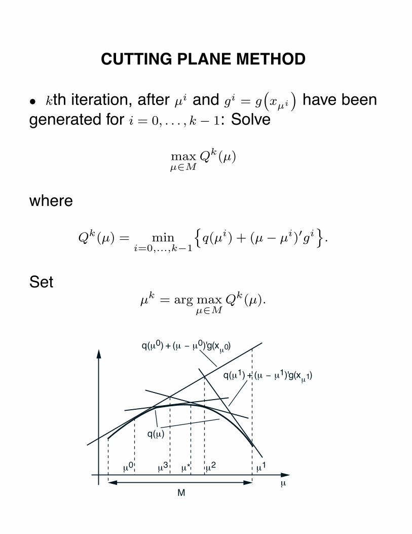
CUTTING PLANE METHOD

• kth iteration, after µi and gi = g(xµi

)have been

generated for i = 0, . . . , k − 1: Solve

maxµ∈M

Qk(µ)

where

Qk(µ) = mini=0,...,k−1

{q(µi) + (µ − µi)′gi

}.

Setµk = arg max

µ∈MQk(µ).

M

q(µ)

µ1µ0 µ2µ3 µ*

µ

q(µ0) + (µ − µ0)'g(x )µ0

q(µ1) + (µ − µ1)'g(x )µ1

POLYHEDRAL CASE

q(µ) = mini∈I

{a′

iµ + bi

}where I is a finite index set, and ai ∈ �r and bi aregiven.

• Then subgradient gk in the cutting plane methodis a vector aik for which the minimum is attained.

• Finite termination expected.

M

q(µ)

µ1µ0 µ2µ3

µµ*µ4

=

CONVERGENCE

• Proposition: Assume that the max of Qk over M

is attained and that q is real-valued. Then everylimit point of a sequence {µk} generated by thecutting plane method is a dual optimal solution.

Proof: gi is a subgradient of q at µi, so

q(µi) + (µ − µi)′gi ≥ q(µ), ∀ µ ∈ M,

Qk(µk) ≥ Qk(µ) ≥ q(µ), ∀ µ ∈ M. (1)

• Suppose {µk}K converges to µ̄. Then, µ̄ ∈ M ,and by Eq. (1) and continuity of Qk and q (real-valued assumption), Qk(µ̄) ≥ q(µ̄). Using this andEq. (1), we obtain for all k and i < k,

q(µi) + (µk − µi)′gi ≥ Qk(µk) ≥ Qk(µ̄) ≥ q(µ̄).

• Take the limit as i → ∞, k → ∞, i ∈ K, k ∈ K,

limk→∞, k∈K

Qk(µk) = q(µ̄).

Combining with (1), q(µ̄) = maxµ∈M q(µ).

LAGRANGIAN RELAXATION

• Solving the dual of the separable problem

minimizeJ∑

j=1

fj(xj)

subject to xj ∈ Xj , j = 1, . . . , J,

J∑j=1

Ajxj = b.

• Dual function is

q(λ) =

J∑j=1

minxj∈Xj

{fj(xj) + λ′Ajxj

}− λ′b

=

J∑j=1

{fj

(xj(λ)

)+ λ′Ajxj(λ)

}− λ′b

where xj(λ) attains the min. A subgradient at λ is

gλ =

J∑j=1

Ajxj(λ) − b.

DANTSIG-WOLFE DECOMPOSITION

• D-W decomposition method is just the cuttingplane applied to the dual problem maxλ q(λ).

• At the kth iteration, we solve the “approximatedual”

λk = arg maxλ∈r

Qk(λ) ≡ mini=0,...,k−1

{q(λi) + (λ − λi)′gi

}.

• Equivalent linear program in v and λ

maximize v

subject to v ≤ q(λi) + (λ − λi)′gi, i = 0, . . . , k − 1

The dual of this (called master problem) is

minimizek−1∑i=0

ξi(q(λi) − λi′gi

)

subject tok−1∑i=0

ξi = 1,

k−1∑i=0

ξigi = 0,

ξi ≥ 0, i = 0, . . . , k − 1,

DANTSIG-WOLFE DECOMPOSITION (CONT.)

• The master problem is written as

minimizeJ∑

j=1

(k−1∑i=0

ξifj

(xj(λ

i)))

subject tok−1∑i=0

ξi = 1,

J∑j=1

Aj

(k−1∑i=0

ξixj(λi)

)= b,

ξi ≥ 0, i = 0, . . . , k − 1.

• The primal cost function terms fj(xj) are ap-proximated by

k−1∑i=0

ξifj

(xj(λ

i))

• Vectors xj are expressed as

k−1∑i=0

ξixj(λi)

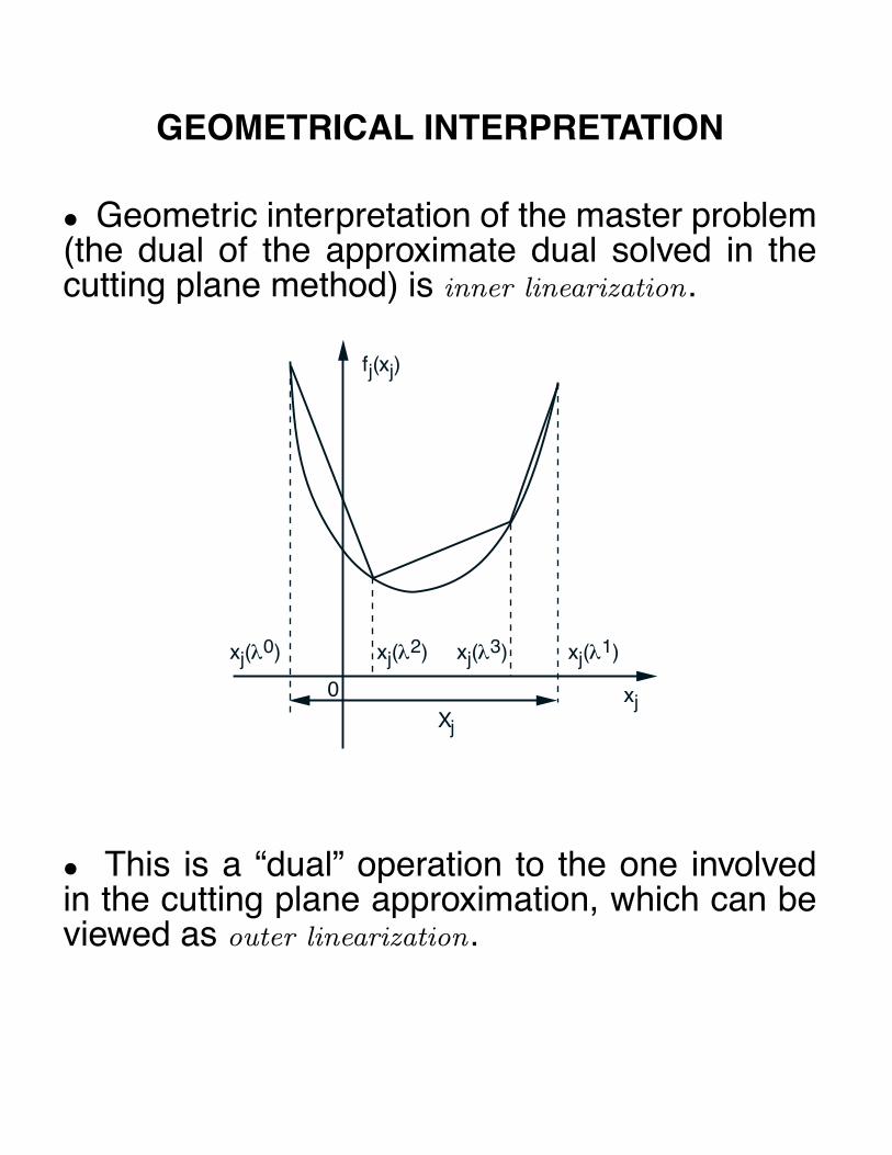
GEOMETRICAL INTERPRETATION

• Geometric interpretation of the master problem(the dual of the approximate dual solved in thecutting plane method) is inner linearization.

0

Xj

fj(xj)

xj

xj(λ0) xj(λ

1)xj(λ2) xj(λ

3)

• This is a “dual” operation to the one involvedin the cutting plane approximation, which can beviewed as outer linearization.


LECTURE 24: EPILOGUE

LECTURE OUTLINE

• Review of three dominant themes from thiscourse

− Descent along feasible directions− Approximation of a “difficult” problem by a

sequence of “easier” problems− Duality

• Discussion of an algorithmic approach that wedid not cover (Sections 4.3, 4.4): Solving the nec-essary optimality conditions, viewed as a systemof equations and inequalities

• More on duality: Relation of primal and dualfunctions

• Connection of constrained optimization dualityand saddle point/game theory

THE DESCENT APPROACH

• Use in necessary optimality conditions: at alocal minimum x∗ of f over X, we have ∇f(x∗)′d ≥ 0

for all feasible directions d of X at x∗. Specialcases:

− ∇f(x∗) = 0 when X = �n

− ∇f(x∗)′(x − x∗) ≥ 0 for all x ∈ X, when X isconvex

• Use in sufficient optimality conditions underHessian positive definiteness, or under convexityassumptions

• Use in algorithms:− Gradient-related methods for unconstrained

optimization− Feasible direction algorithms− Subgradient methods (based on descent of

the distance of the current iterate to the op-timum)

THE APPROXIMATION APPROACH

• Use in Lagrange multiplier theory:− Introduce a penalized problem that “converges”

to the original constrained problem as thepenalty parameter goes to ∞

− Take the limit in the optimality conditions forthe penalized problem to obtain optimalityconditions for the constrained problem

• Also use in sufficient optimality conditions usingan augmented Lagrangian approach

• Use in algorithms:− Barrier/interior point methods− Penalty and augmented Lagrangian meth-

ods− Cutting plane methods

SOLVING THE NECESSARY CONDITIONS

• Another algorithmic approach for equality andinequality constrained problems (we did not coverit; see Sections 4.3, 4.4). It is based on:

− Viewing the optimality (KKT) conditions as asystem of (nonlinear) equations and inequal-ities to be solved for x and the multipliers

− Solving them using some method for solvingsystems of equations and inequalities

• Principal solution methods are a number of vari-ants of Newton’s method

• Important issue: how to enlarge the region ofconvergence of Newton’s method without destroy-ing its fast convergence near a solution

• Principal tools: stepsize procedures and meritfunctions

• Important methods:− Sequential quadratic programming (Section

4.3)− Primal-dual interior point methods (Section

4.4)

DUALITY - MIN COMMON/MAX CROSSING

• The principal issues in constrained optimiza-tion duality are intuitively captured in the min com-mon/max crossing framework, including:

− The weak duality theorem− The need for convexity assumptions in order

that there is no duality gap− The Slater condition, which guarantees the

existence of a geometric multiplier− The pathologies that can result in a duality

gap, even under convexity conditions

• For the problem minx∈X, g(x)≤0 f(x), an importantconcept is the primal function, defined by

p(u) = infx∈X, g(x)≤u

f(x)

• If X, f , and gj are convex, then it can be shownthat p is convex

• Assuming convexity of p

− The set of geometric multipliers is equal tothe set of subgradients of p at 0

− Absence of a duality gap is equivalent toright continuity of p at 0, i.e., p(0) = limu↓0 p(u)

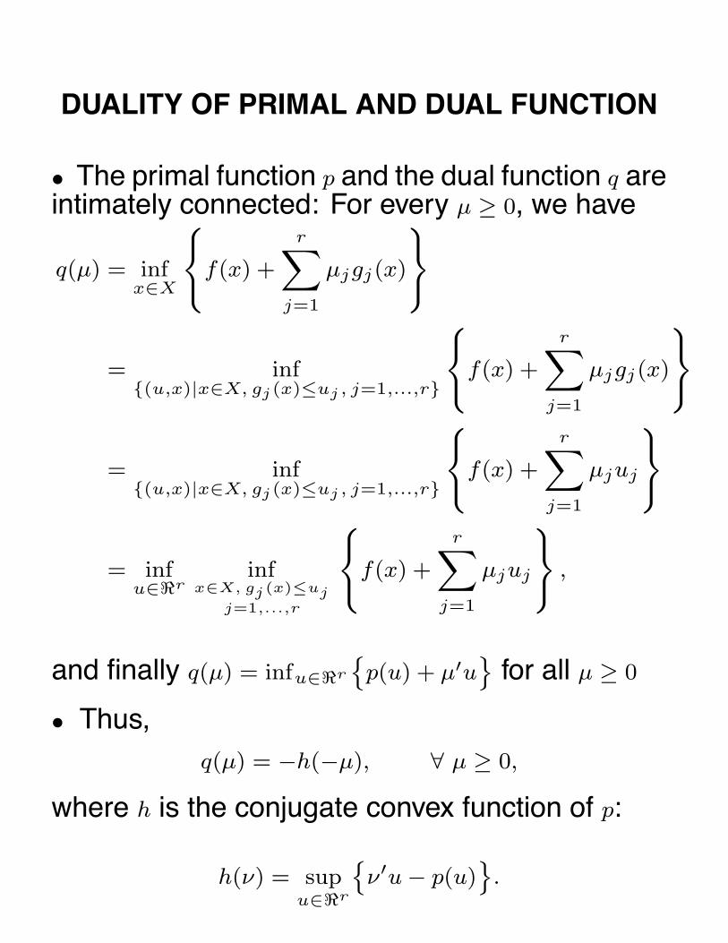
DUALITY OF PRIMAL AND DUAL FUNCTION

• The primal function p and the dual function q areintimately connected: For every µ ≥ 0, we have

q(µ) = infx∈X

{f(x) +

r∑j=1

µjgj(x)

}

= inf{(u,x)|x∈X, gj(x)≤uj , j=1,...,r}

{f(x) +

r∑j=1

µjgj(x)

}

= inf{(u,x)|x∈X, gj(x)≤uj , j=1,...,r}

{f(x) +

r∑j=1

µjuj

}

= infu∈r

infx∈X, gj(x)≤uj

j=1,...,r

{f(x) +

r∑j=1

µjuj

},

and finally q(µ) = infu∈r

{p(u) + µ′u

}for all µ ≥ 0

• Thus,q(µ) = −h(−µ), ∀ µ ≥ 0,

where h is the conjugate convex function of p:

h(ν) = supu∈r

{ν′u − p(u)

}.

DUALITY AND MINIMAX THEORY

• Duality issues for the problem minx∈X, g(x)≤0 f(x)

are closely connected to saddle point issues forthe Lagrangian function

L(x, µ) = f(x) + µ′g(x)

• We have

f∗ = infx∈X, g(x)≤0

f(x) = infx∈X

supµ≥0

L(x, µ),

q∗ = supµ≥0

q(µ) = supµ≥0

infx∈X

L(x, µ),

so no duality gap is equivalent to

infx∈X

supµ≥0

L(x, µ) = supµ≥0

infx∈X

L(x, µ)

• Also, we showed that (x, µ) is a global minimum-geometric multiplier pair if and only if it is a saddlepoint of L(x, µ) over x ∈ X and µ ≥ 0

• Constrained optimization duality theory can beviewed as the special case of minimax theory whereµ appears linearly and is constrained by µ ≥ 0; butgeneral minimax theory does not shed much lighton this special case

COMMON ROOT OF DUALITY AND MINIMAX

• Constrained optimization duality theory and min-imax theory are not “equivalent” but they have acommon geometrical root: the min common/maxcrossing structure

• Consider the issue whether infx∈X supµ∈M φ(x, µ) =

supµ∈M infx∈X φ(x, µ) and letp(u) = inf

x∈Xsup

µ∈M

{φ(x, µ) − u′µ

}[If φ(x, µ) = L(x, µ), p is equal to the primal function.]

• Consider also the min common/max crossingframework for the set {(u, w) | p(u) ≤ w

}. Then the

min common value is p(0) = infx∈X supµ∈M φ(x, µ)

• Under convexity/semicontinuity assumptions onX, M , φ(·, µ), and −φ(x, ·), it can be shown that themax crossing value is equal to supµ∈M infx∈X φ(x, µ)

• Thus equality of the min common and maxcrossing values is equivalent to

infx∈X

supµ∈M

φ(x, µ) = supµ∈M

infx∈X

φ(x, µ)

• For an extensive analysis of all this, see theauthor’s book “Convex Analysis and Optimization”

http://www.athenasc.com/convexity.html

lecture slides on nonlinear programming … · lecture slides on nonlinear programming based on...

Documents