lecture: vector semantics (aka distributional semantics)
TRANSCRIPT
Seman&c Analysis in Language Technology http://stp.lingfil.uu.se/~santinim/sais/2016/sais_2016.htm
Vector Semantics
(aka Distributional Semantics)
Marina San(ni [email protected]
Department of Linguis(cs and Philology
Uppsala University, Uppsala, Sweden
Spring 2016
1

Previous Lecture: Word Sense Disambigua$on
2

Similarity measures (dic$onary-‐based)
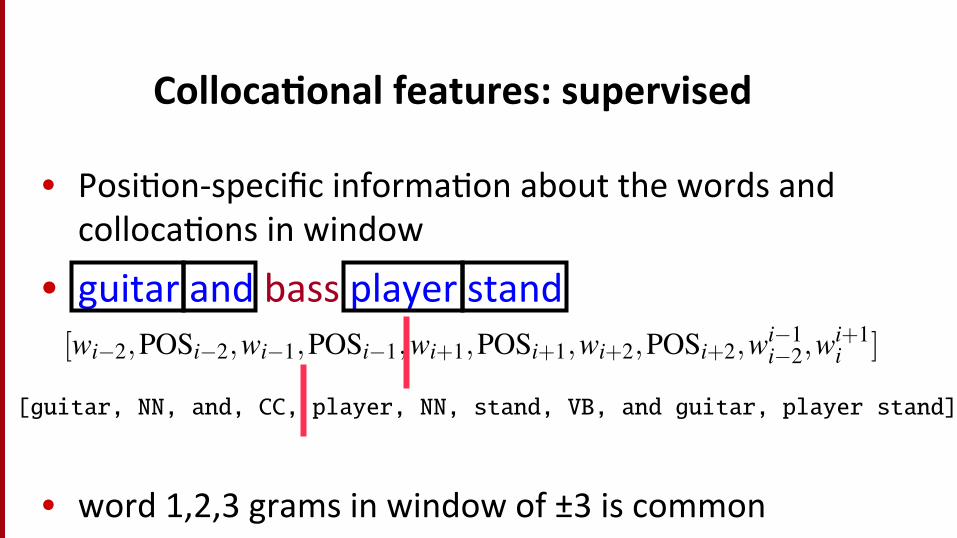
Colloca$onal features: supervised
• Posi(on-‐specific informa(on about the words and colloca(ons in window
• guitar and bass player stand
• word 1,2,3 grams in window of ±3 is common
10 CHAPTER 16 • COMPUTING WITH WORD SENSES
ually tagged with WordNet senses (Miller et al. 1993, Landes et al. 1998). In ad-dition, sense-tagged corpora have been built for the SENSEVAL all-word tasks. TheSENSEVAL-3 English all-words test data consisted of 2081 tagged content word to-kens, from 5,000 total running words of English from the WSJ and Brown corpora(Palmer et al., 2001).
The first step in supervised training is to extract features that are predictive ofword senses. The insight that underlies all modern algorithms for word sense disam-biguation was famously first articulated by Weaver (1955) in the context of machinetranslation:
If one examines the words in a book, one at a time as through an opaquemask with a hole in it one word wide, then it is obviously impossibleto determine, one at a time, the meaning of the words. [. . . ] But ifone lengthens the slit in the opaque mask, until one can see not onlythe central word in question but also say N words on either side, thenif N is large enough one can unambiguously decide the meaning of thecentral word. [. . . ] The practical question is : “What minimum value ofN will, at least in a tolerable fraction of cases, lead to the correct choiceof meaning for the central word?”
We first perform some processing on the sentence containing the window, typi-cally including part-of-speech tagging, lemmatization , and, in some cases, syntacticparsing to reveal headwords and dependency relations. Context features relevant tothe target word can then be extracted from this enriched input. A feature vectorfeature vectorconsisting of numeric or nominal values encodes this linguistic information as aninput to most machine learning algorithms.
Two classes of features are generally extracted from these neighboring contexts,both of which we have seen previously in part-of-speech tagging: collocational fea-tures and bag-of-words features. A collocation is a word or series of words in acollocationposition-specific relationship to a target word (i.e., exactly one word to the right, orthe two words starting 3 words to the left, and so on). Thus, collocational featurescollocational
featuresencode information about specific positions located to the left or right of the targetword. Typical features extracted for these context words include the word itself, theroot form of the word, and the word’s part-of-speech. Such features are effective atencoding local lexical and grammatical information that can often accurately isolatea given sense.
For example consider the ambiguous word bass in the following WSJ sentence:(16.17) An electric guitar and bass player stand off to one side, not really part of
the scene, just as a sort of nod to gringo expectations perhaps.A collocational feature vector, extracted from a window of two words to the rightand left of the target word, made up of the words themselves, their respective parts-of-speech, and pairs of words, that is,
[wi�2,POSi�2,wi�1,POSi�1,wi+1,POSi+1,wi+2,POSi+2,wi�1i�2,w
i+1i ] (16.18)
would yield the following vector:[guitar, NN, and, CC, player, NN, stand, VB, and guitar, player stand]
High performing systems generally use POS tags and word collocations of length1, 2, and 3 from a window of words 3 to the left and 3 to the right (Zhong and Ng,2010).
The second type of feature consists of bag-of-words information about neigh-boring words. A bag-of-words means an unordered set of words, with their exactbag-of-words

Bag-‐of-‐words features: supervised
• Assume we’ve seGled on a possible vocabulary of 12 words in “bass” sentences:
[fishing, big, sound, player, fly, rod, pound, double, runs, playing, guitar, band]
• The vector for: guitar and bass player stand [0,0,0,1,0,0,0,0,0,0,1,0]
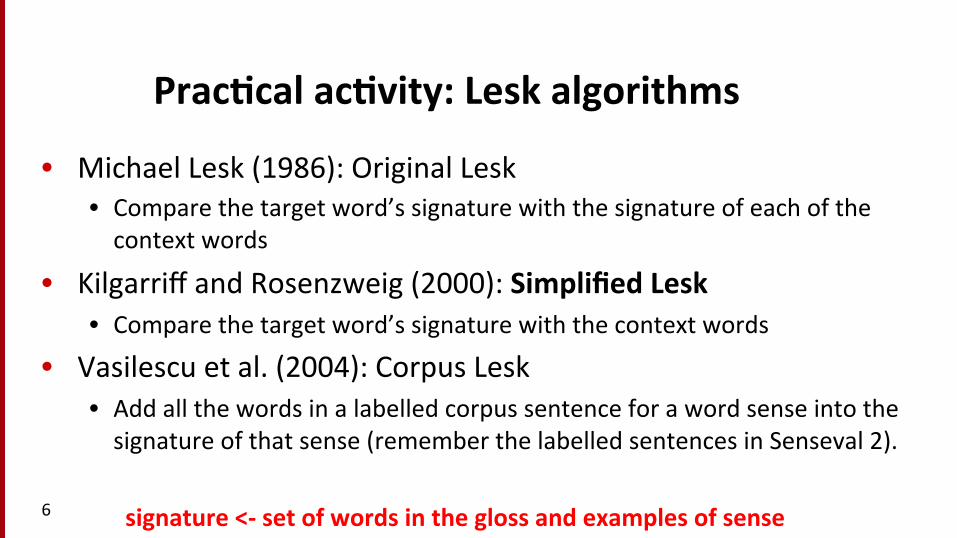
Prac$cal ac$vity: Lesk algorithms
• Michael Lesk (1986): Original Lesk • Compare the target word’s signature with the signature of each of the context words
• Kilgarriff and Rosenzweig (2000): Simplified Lesk • Compare the target word’s signature with the context words
• Vasilescu et al. (2004): Corpus Lesk • Add all the words in a labelled corpus sentence for a word sense into the signature of that sense (remember the labelled sentences in Senseval 2).
signature <-‐ set of words in the gloss and examples of sense 6

Simplified Lesk: Time flies like an arrow
• Common sense:
• Modern English speakers unambiguously understand the sentence to mean "As a generalisa(on, (me passes in the same way that an arrow generally flies (i.e. quickly)" (as in the common metaphor 5me goes by quickly).
7

Ref: wikipedia • But formally/logically/syntactally/seman(cally à ambiguous:
1. (as an impera(ve) Measure the speed of flies like you would measure that of an arrow -‐ i.e. (You should) (me flies as you would (me an arrow.
2. (impera(ve) Measure the speed of flies like an arrow would -‐ i.e. (You should) (me flies in the same manner that an arrow would (me them.
3. (impera(ve) Measure the speed of flies that are like arrows -‐ i.e. (You should) (me those flies that are like an arrow.
4. (declara(ve) Time moves in a way an arrow would. 5. (declara(ve, i.e. neutrally sta(ng a proposi(on) Certain flying insects,
"(me flies," enjoy an arrow.
•
8

Simplified Lesk algorithm (2000) and WordNet (3.1)
• Disambigua(ng $me : • (me#n#5 shares ”pass” and ”$me flies as an arrow” with flies#v#8
• Disambigua(ng flies • flies#v#8 shares ”pass” and ”$me flies as an arrow” with (me#v#5
So we select the following senses: (me#n#5 and flies#v#8.
9
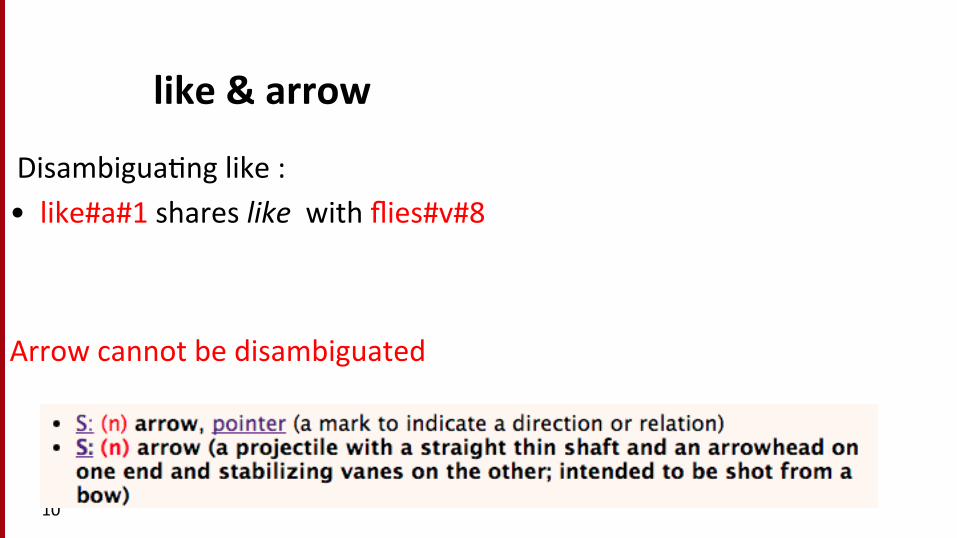
like & arrow
Disambigua(ng like : • like#a#1 shares like with flies#v#8 Arrow cannot be disambiguated
10

11
Similar a#3
like a#1
fly v#8
Time n#5

Corpus Lesk Algorithm • Expands the approach by:
• Adding all the words of any sense-‐tagged corpus data (like SemCor) for a word sense into the signature for that sense.
• Signature= gloss+examples of a word sense
12
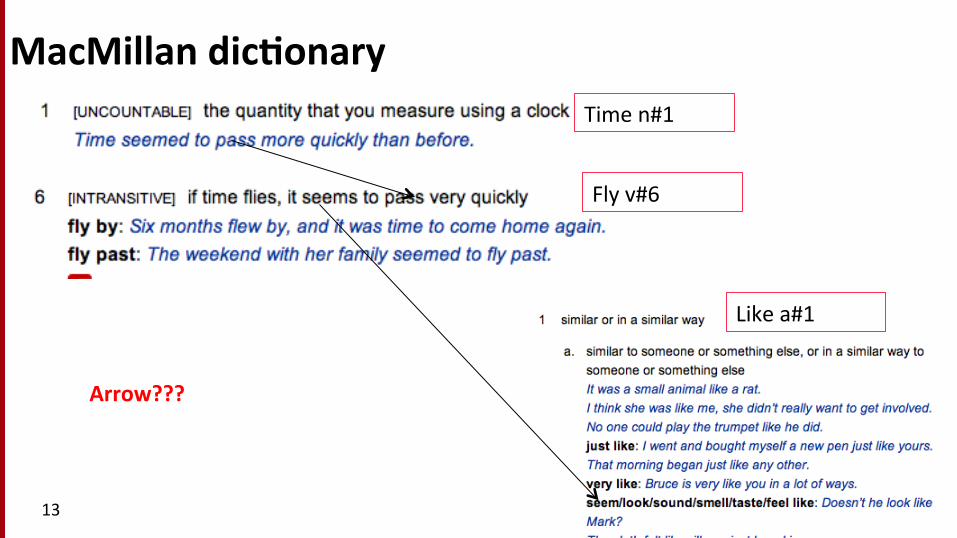
MacMillan dic$onary
13
Arrow???
Time n#1
Fly v#6
Like a#1

Arrow ???
14
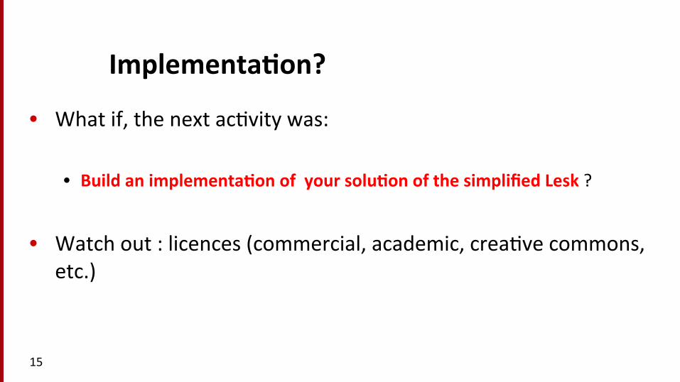
Implementa$on?
• What if, the next ac(vity was:
• Build an implementa$on of your solu$on of the simplified Lesk ?
• Watch out : licences (commercial, academic, crea(ve commons, etc.)
15
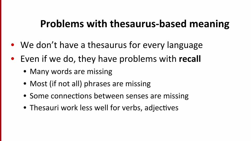
Problems with thesaurus-‐based meaning
• We don’t have a thesaurus for every language • Even if we do, they have problems with recall
• Many words are missing • Most (if not all) phrases are missing • Some connec(ons between senses are missing • Thesauri work less well for verbs, adjec(ves

End of previous lecture
17
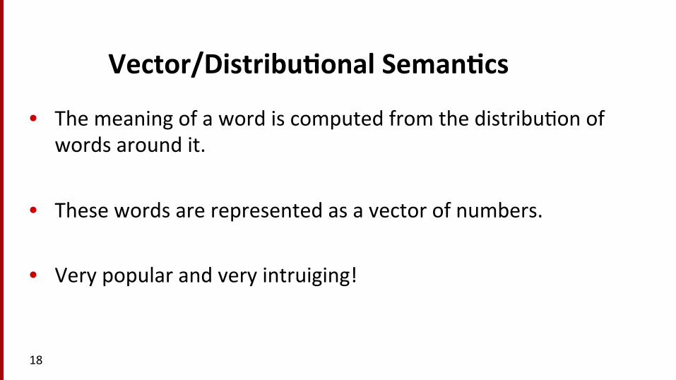
Vector/Distribu$onal Seman$cs
• The meaning of a word is computed from the distribu(on of words around it.
• These words are represented as a vector of numbers.
• Very popular and very intruiging!
18

hZp://esslli2016.unibz.it/?page_id=256
19

(Oversimplified) Preliminaries (cf also Lect 03: SA, Turney Algorithm)
• Probability • Joint probability • Marginals • PMI • PPMI • Smoothing • Dot product (aka inner product) • Window 20

Probability
• Probability is the measure of how likely an event is.
21
Ex: John has a box with a book, a map and a ruler in it (Cantos Gomez, 2013) This sentence has 14 words and 5 nouns. The probability of picking up a noun is: P(noun)= 5/14 = 0.357
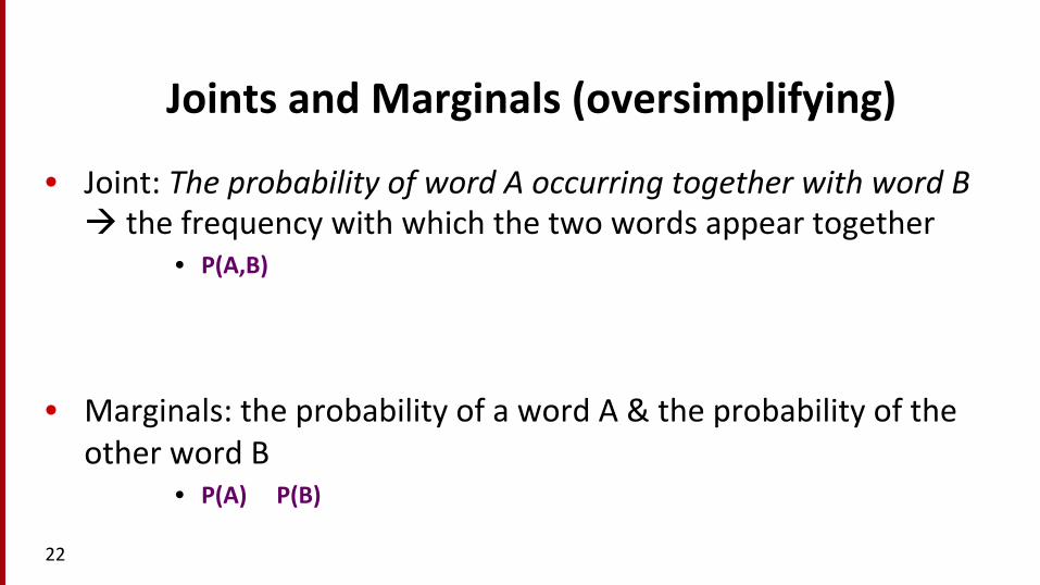
Joints and Marginals (oversimplifying)
• Joint: The probability of word A occurring together with word B à the frequency with which the two words appear together
• P(A,B)
• Marginals: the probability of a word A & the probability of the other word B
• P(A) P(B)
22

Can also be said in other ways: Dependent and independent events: Joints & Marginals
• Two events are dependent if the outcome or occurrence of the first affects the outcome or occurrence of the second so that the probability is changed. • Consider two dependent events, A and B. The joint probability that A and B occur together is :
• P(A and B) = P(A)*P(B given A) OR P(A and B) = P(B)*P(A given B) • Two events are independent, each probability is mul(plied
together to find the overall probability for the set of events. • P(A and B) = P(A)*P(B)
Marginal probability is the probability of the occurrence of a single event in joint probability. 23
Equivalent Nota(ons (joint) • P(A,B) or P(A ∩B)

Associa$on measure
• Pointwise mutual informa$on: • How much more do events x and y co-‐occur than if they were independent?
Read: the joint probability of two dependent events (ie, the 2 words that are supposed to be associated) divided by the product of the individual probabili(es (ie, we assume that the words are not associated, we assume they are independent), and we take the log of it. It tells us how much more the two events co-‐occur than if they were independent
PMI(X,Y ) = log2P(x,y)P(x)P(y)
POSITIVE PMI
• We replace all the nega(ve values with 0.
25

Smoothing (addi$ve, Laplace, etc.)
• In very simple words: we add an arbitrary value to the counts.
• In a bag of words model of natural language processing and informa(on retrieval, addi(ve smoothing allows the assignment of non-‐zero probabili(es to words which do not occur in the sample à data sparsenessà mul(plica(on by 0 probability: all the counts are 0.
• (Addi(ve smoothing is commonly a component of naive Bayes classifiers. 26

Dot product (aka inner product)
• Given the two vectors:
• The dot product is :
• The Dot Product is wriGen using a central dot
27
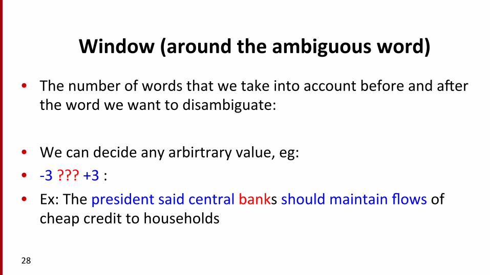
Window (around the ambiguous word)
• The number of words that we take into account before and axer the word we want to disambiguate:
• We can decide any arbirtrary value, eg: • -‐3 ??? +3 : • Ex: The president said central banks should maintain flows of
cheap credit to households
28

Acknowledgements Most slides borrowed or adapted from:
Dan Jurafsky and James H. Mar(n
Dan Jurafsky and Christopher Manning, Coursera
J&M(2015, drax): hGps://web.stanford.edu/~jurafsky/slp3/

Distributional Semantics Term-‐context matrix
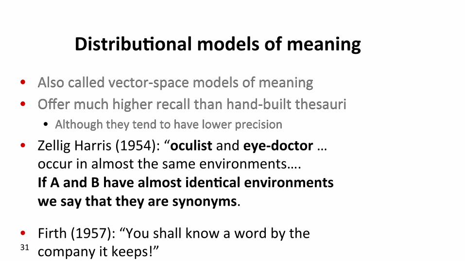
Distribu$onal models of meaning
• Also called vector-‐space models of meaning • Offer much higher recall than hand-‐built thesauri
• Although they tend to have lower precision • Zellig Harris (1954): “oculist and eye-‐doctor …
occur in almost the same environments…. If A and B have almost iden$cal environments we say that they are synonyms.
• Firth (1957): “You shall know a word by the company it keeps!” 31
• Also called vector-‐space models of meaning • Offer much higher recall than hand-‐built thesauri
• Although they tend to have lower precision
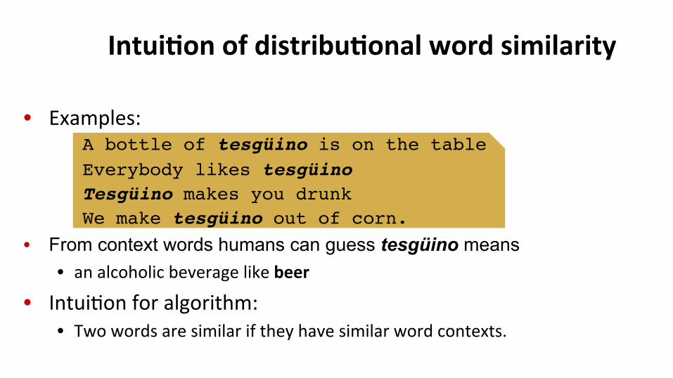
Intui$on of distribu$onal word similarity
• Examples: A bottle of tesgüino is on the table!Everybody likes tesgüino!Tesgüino makes you drunk!We make tesgüino out of corn.!
• From context words humans can guess tesgüino means • an alcoholic beverage like beer
• Intui(on for algorithm: • Two words are similar if they have similar word contexts.
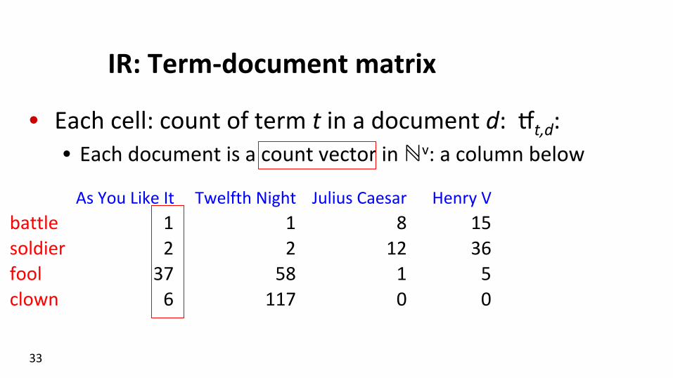
As#You#Like#It Twelfth#Night Julius#Caesar Henry#Vbattle 1 1 8 15soldier 2 2 12 36fool 37 58 1 5clown 6 117 0 0
IR: Term-‐document matrix
• Each cell: count of term t in a document d: |t,d: • Each document is a count vector in ℕv: a column below
33
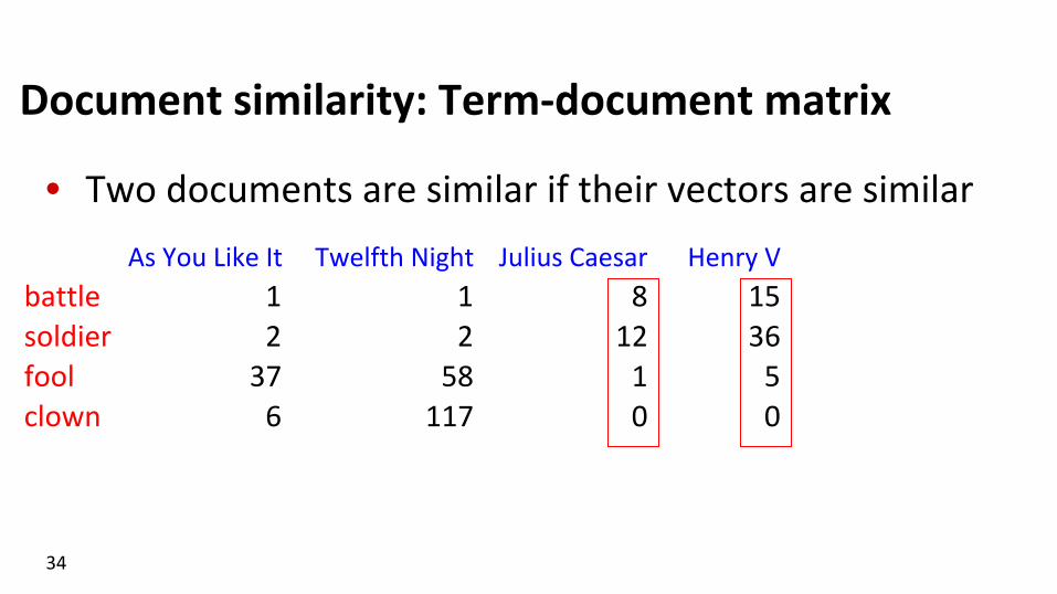
Document similarity: Term-‐document matrix
• Two documents are similar if their vectors are similar
34
As#You#Like#It Twelfth#Night Julius#Caesar Henry#Vbattle 1 1 8 15soldier 2 2 12 36fool 37 58 1 5clown 6 117 0 0
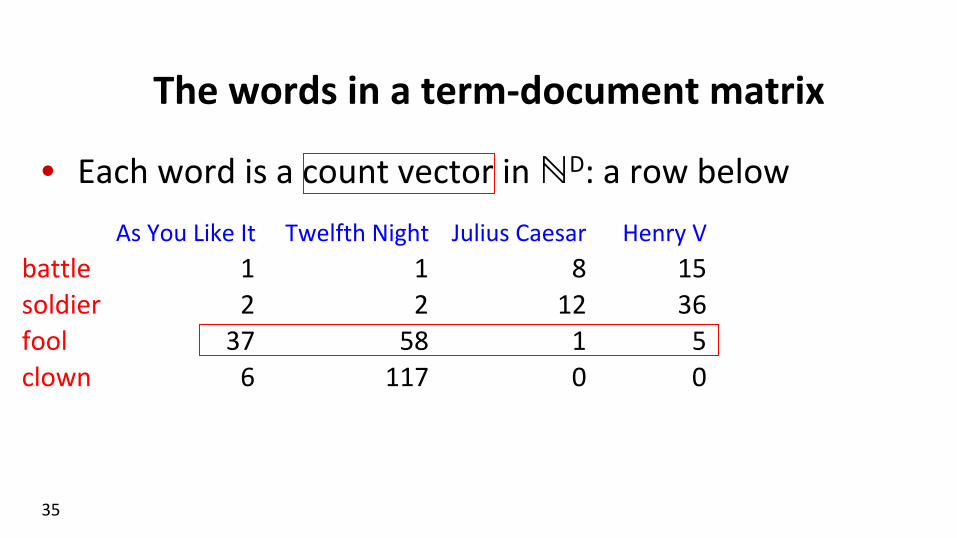
The words in a term-‐document matrix
• Each word is a count vector in ℕD: a row below
35
As#You#Like#It Twelfth#Night Julius#Caesar Henry#Vbattle 1 1 8 15soldier 2 2 12 36fool 37 58 1 5clown 6 117 0 0
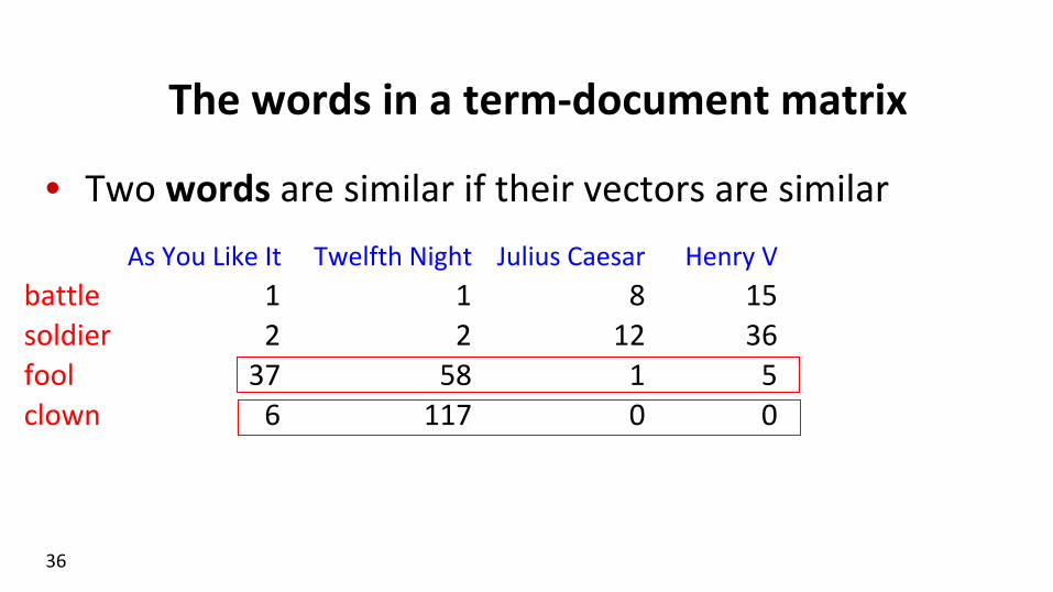
The words in a term-‐document matrix
• Two words are similar if their vectors are similar
36
As#You#Like#It Twelfth#Night Julius#Caesar Henry#Vbattle 1 1 8 15soldier 2 2 12 36fool 37 58 1 5clown 6 117 0 0

The intui$on of distribu$onal word similarity…
• Instead of using en(re documents, use smaller contexts • Paragraph • Window of 10 words
• A word is now defined by a vector over counts of context words
37
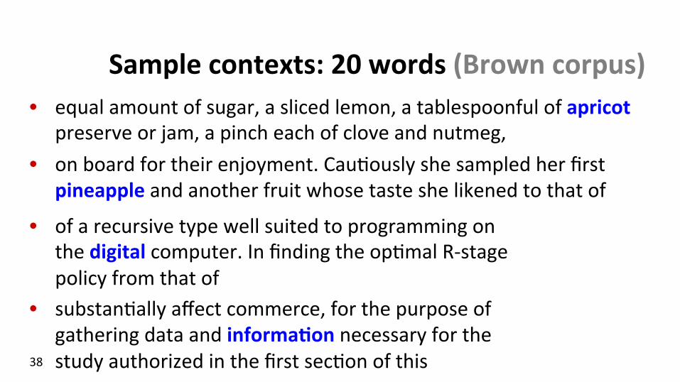
Sample contexts: 20 words (Brown corpus) • equal amount of sugar, a sliced lemon, a tablespoonful of apricot
preserve or jam, a pinch each of clove and nutmeg, • on board for their enjoyment. Cau(ously she sampled her first
pineapple and another fruit whose taste she likened to that of
38
• of a recursive type well suited to programming on the digital computer. In finding the op(mal R-‐stage policy from that of
• substan(ally affect commerce, for the purpose of gathering data and informa$on necessary for the study authorized in the first sec(on of this

Term-‐context matrix for word similarity
• Two words are similar in meaning if their context vectors are similar
39
aardvark computer data pinch result sugar …apricot 0 0 0 1 0 1pineapple 0 0 0 1 0 1digital 0 2 1 0 1 0information 0 1 6 0 4 0

Should we use raw counts?
• For the term-‐document matrix • We used |-‐idf instead of raw term counts
• For the term-‐context matrix • Posi(ve Pointwise Mutual Informa(on (PPMI) is common
40
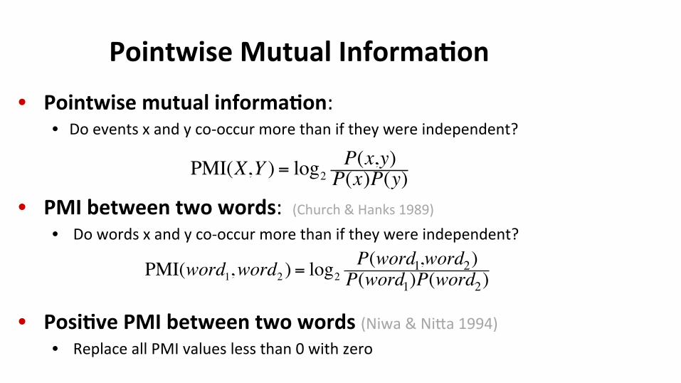
Pointwise Mutual Informa$on
• Pointwise mutual informa$on: • Do events x and y co-‐occur more than if they were independent?
• PMI between two words: (Church & Hanks 1989) • Do words x and y co-‐occur more than if they were independent?
• Posi$ve PMI between two words (Niwa & NiGa 1994) • Replace all PMI values less than 0 with zero
PMI(X,Y ) = log2P(x,y)P(x)P(y)
PMI(word1,word2 ) = log2P(word1,word2)P(word1)P(word2)
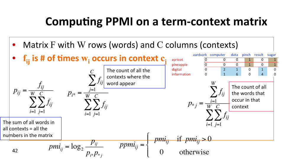
Compu$ng PPMI on a term-‐context matrix
• Matrix F with W rows (words) and C columns (contexts) • fij is # of $mes wi occurs in context cj
42
pij =fij
fijj=1
C
∑i=1
W
∑pi* =
fijj=1
C
∑
fijj=1
C
∑i=1
W
∑ p* j =fij
i=1
W
∑
fijj=1
C
∑i=1
W
∑
pmiij = log2pij
pi*p* jppmiij =
pmiij if pmiij > 0
0 otherwise
!"#
$#
The count of all the words that occur in that context
The count of all the contexts where the word appear
The sum of all words in all contexts = all the numbers in the matrix
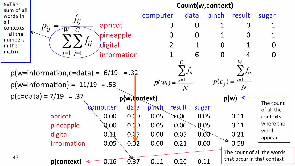
p(w=informa(on,c=data) = p(w=informa(on) = p(c=data) =
43
= .32 6/19
11/19 = .58
7/19 = .37
pij =fij
fijj=1
C
∑i=1
W
∑
p(wi ) =fij
j=1
C
∑
Np(cj ) =
fiji=1
W
∑
N
The count of all the words that occur in that context
The count of all the contexts where the word appear
N=The sum of all words in all contexts = all the numbers in the matrix
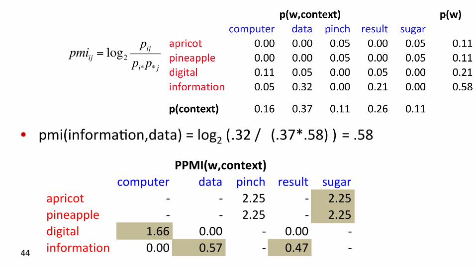
44
pmiij = log2pij
pi*p* j
• pmi(informa(on,data) = log2 (
PPMI(w,context)computer data pinch result sugar
apricot 1 1 2.25 1 2.25pineapple 1 1 2.25 1 2.25digital 1.66 0.00 1 0.00 1information 0.00 0.57 1 0.47 1
.32 / (.37*.58) ) = .58
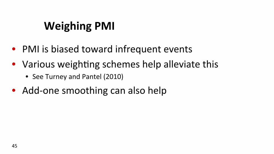
Weighing PMI
• PMI is biased toward infrequent events • Various weigh(ng schemes help alleviate this
• See Turney and Pantel (2010)
• Add-‐one smoothing can also help
45

46
Add#2%Smoothed%Count(w,context)computer data pinch result sugar
apricot 2 2 3 2 3pineapple 2 2 3 2 3digital 4 3 2 3 2information 3 8 2 6 2
p(w,context),[add02] p(w)computer data pinch result sugar
apricot 0.03 0.03 0.05 0.03 0.05 0.20pineapple 0.03 0.03 0.05 0.03 0.05 0.20digital 0.07 0.05 0.03 0.05 0.03 0.24information 0.05 0.14 0.03 0.10 0.03 0.36
p(context) 0.19 0.25 0.17 0.22 0.17

Original vs add-‐2 smoothing
47
PPMI(w,context).[add22]computer data pinch result sugar
apricot 0.00 0.00 0.56 0.00 0.56pineapple 0.00 0.00 0.56 0.00 0.56digital 0.62 0.00 0.00 0.00 0.00information 0.00 0.58 0.00 0.37 0.00
PPMI(w,context)computer data pinch result sugar
apricot 1 1 2.25 1 2.25pineapple 1 1 2.25 1 2.25digital 1.66 0.00 1 0.00 1information 0.00 0.57 1 0.47 1
Distributional Semantics Dependency rela(ons

Using syntax to define a word’s context • Zellig Harris (1968)
• “The meaning of en((es, and the meaning of gramma(cal rela(ons among them, is related to the restric(on of combina(ons of these en((es rela(ve to other en((es”
• Two words are similar if they have similar parse contexts • Duty and responsibility (Chris Callison-‐Burch’s example)
Modified by adjec$ves
addi(onal, administra(ve, assumed, collec(ve, congressional, cons(tu(onal …
Objects of verbs assert, assign, assume, aGend to, avoid, become, breach …
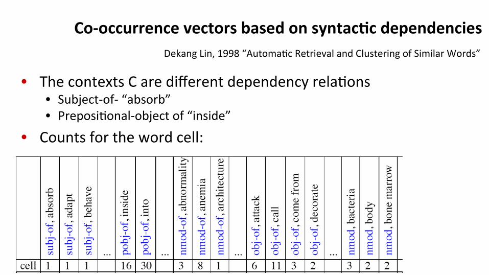
Co-‐occurrence vectors based on syntac$c dependencies
• The contexts C are different dependency rela(ons • Subject-‐of-‐ “absorb” • Preposi(onal-‐object of “inside”
• Counts for the word cell:
Dekang Lin, 1998 “Automa(c Retrieval and Clustering of Similar Words”
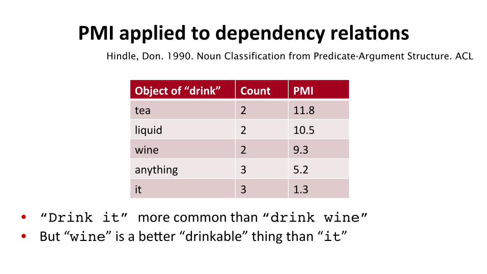
PMI applied to dependency rela$ons
• “Drink it” more common than “drink wine”!• But “wine” is a beGer “drinkable” thing than “it”
Object of “drink” Count PMI
it 3 1.3
anything 3 5.2
wine 2 9.3
tea 2 11.8
liquid 2 10.5
Hindle, Don. 1990. Noun Classification from Predicate-Argument Structure. ACL
Object of “drink” Count PMI
tea 2 11.8
liquid 2 10.5
wine 2 9.3
anything 3 5.2
it 3 1.3

Cosine for compu$ng similarity
cos(v, w) =v • wv w
=vv•ww=
viwii=1
N∑vi2
i=1
N∑ wi
2i=1
N∑
Dot product Unit vectors
vi is the PPMI value for word v in context i wi is the PPMI value for word w in context i. Cos(v,w) is the cosine similarity of v and w
Sec. 6.3
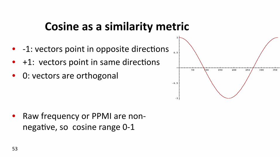
Cosine as a similarity metric
• -‐1: vectors point in opposite direc(ons • +1: vectors point in same direc(ons • 0: vectors are orthogonal
• Raw frequency or PPMI are non-‐nega(ve, so cosine range 0-‐1
53

large data computer apricot 1 0 0 digital 0 1 2 informa(on 1 6 1
54
Which pair of words is more similar? cosine(apricot,informa(on) = cosine(digital,informa(on) = cosine(apricot,digital) =
cos(v, w) =v • wv w
=vv•ww=
viwii=1
N∑vi2
i=1
N∑ wi
2i=1
N∑
1+ 0+ 0
1+ 0+ 0
1+36+1
1+36+1
0+1+ 4
0+1+ 4
1+ 0+ 0
0+ 6+ 2
0+ 0+ 0
=138
= .16
=838 5
= .58
= 0

Other possible similarity measures

The end