lecture8 xing

Eric Xing © Eric Xing @ CMU, 2006-2010 1

Machine Learning

Spectral Clustering

Eric Xing

Lecture 8, August 13, 2010

Reading:


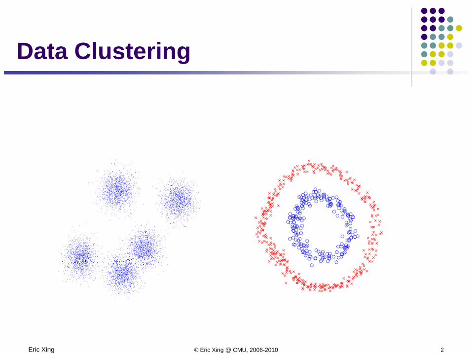
Data Clustering


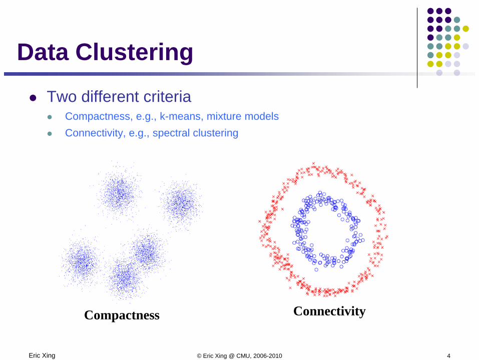
Data Clustering

Compactness Connectivity

Two different criteria Compactness, e.g., k-means, mixture models Connectivity, e.g., spectral clustering


Spectral Clustering

Data Similarities


Some graph terminology Objects (e.g., pixels, data points)

i∈ I = vertices of graph G

Edges (ij) = pixel pairs with Wij > 0

Similarity matrix W = [ Wij ]

Degree di = Σj∈G Wij

dA = Σi∈A di degree of A G

Assoc(A,B) = Σi∈A Σj∈B Wij

⊆

Wiji

j

i

A

AB

Weighted Graph Partitioning


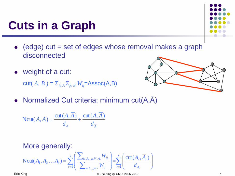
(edge) cut = set of edges whose removal makes a graph disconnected

weight of a cut: cut( A, B ) = Σi∈A Σj∈B Wij=Assoc(A,B)

Normalized Cut criteria: minimum cut(A,Ā)

More generally:

Cuts in a Graph

AA dAA

dAAAA ),(cut),(cut),Ncut( +=

∑∑ ∑∑

== ∈∈

∈∈

=

=

k

r A

rrk

r VjAi ij

AVjAi ijk

rr

rr

dAA

W

WAAA

1121

),(cut),Ncut(,

\,


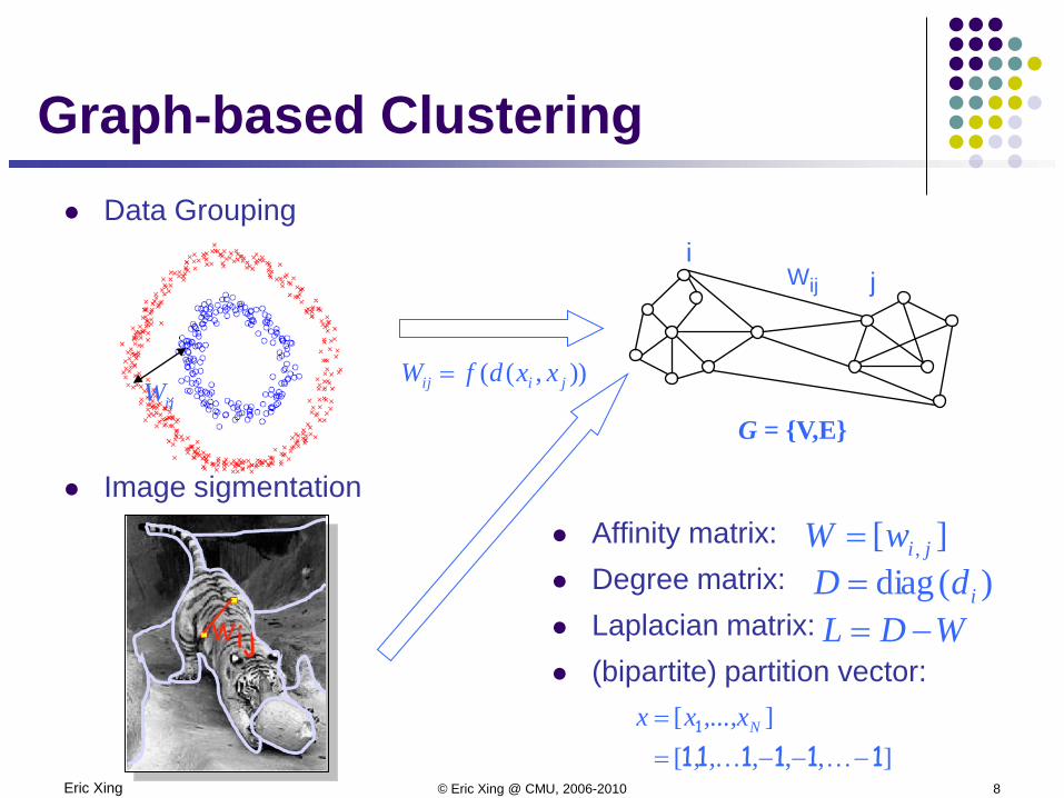
Graph-based Clustering Data Grouping

Image sigmentation Affinity matrix: Degree matrix: Laplacian matrix: (bipartite) partition vector:

ijWG = {V,E}

Wiji

j

)),(( jiij xxdfW =

][ , jiwW =)(diag idD =

WDL −=

],,,[][

1111111

−−−==

,,,...,xxx N


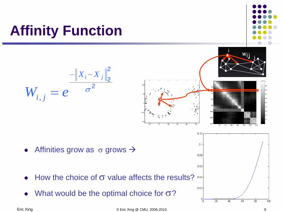
Affinity Function

Affinities grow as σ grows

How the choice of σ value affects the results?

What would be the optimal choice for σ?

2

2

2σ

ji XX

ji eW−−

=,


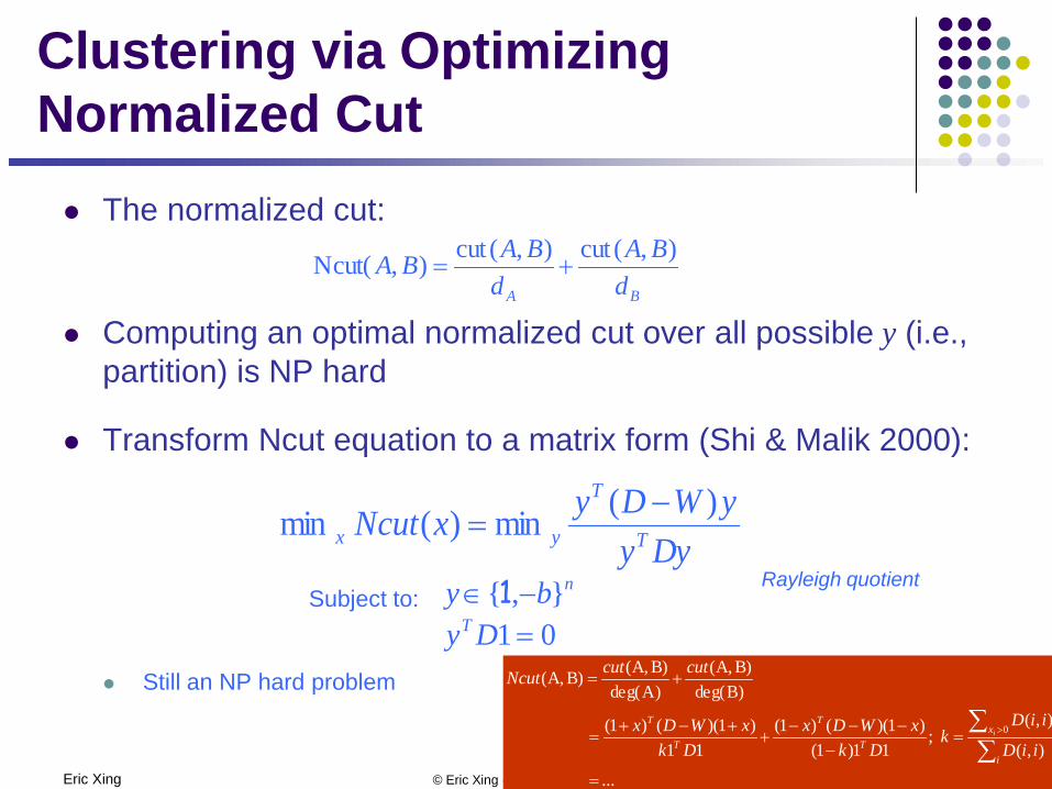
Clustering via Optimizing Normalized Cut The normalized cut:

Computing an optimal normalized cut over all possible y (i.e., partition) is NP hard

Transform Ncut equation to a matrix form (Shi & Malik 2000):

Still an NP hard problem

BA dBA

dBABA ),(cut),(cut),Ncut( +=

DyyyWDyxNcut T

T

yx)(min)(min −

=

01=DyTSubject to:

Rayleigh quotientnby },{ −∈ 1

...

),(

),( ;

11)1()1)(()1(

11)1)(()1(

)Bdeg(B)A,(

)Adeg(B)A,(B)A,(

0

=

=−

−−−+

+−+=

+=

∑∑ >

i

xT

T

T

T

iiD

iiDk

DkxWDx

DkxWDx

cutcutNcut

i


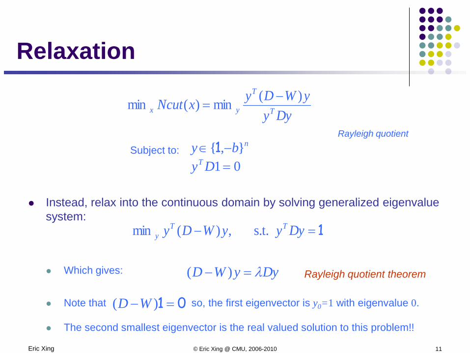
Instead, relax into the continuous domain by solving generalized eigenvalue system:

Which gives:

Note that so, the first eigenvector is y0=1 with eigenvalue 0.

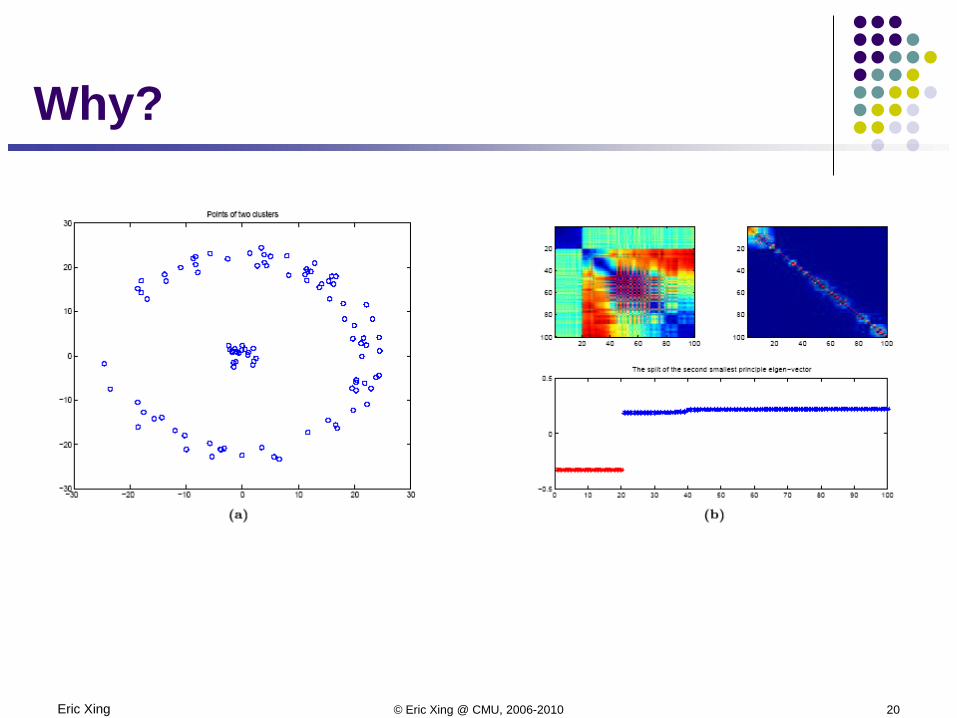
The second smallest eigenvector is the real valued solution to this problem!!

Relaxation

DyyWD λ=− )(

01 =− )( WD

DyyyWDyxNcut T

T

yx)(min)(min −

=

01=DyTSubject to:

Rayleigh quotientnby },{ −∈ 1

1=− DyyyWDy TTy s.t. ,)(min

Rayleigh quotient theorem


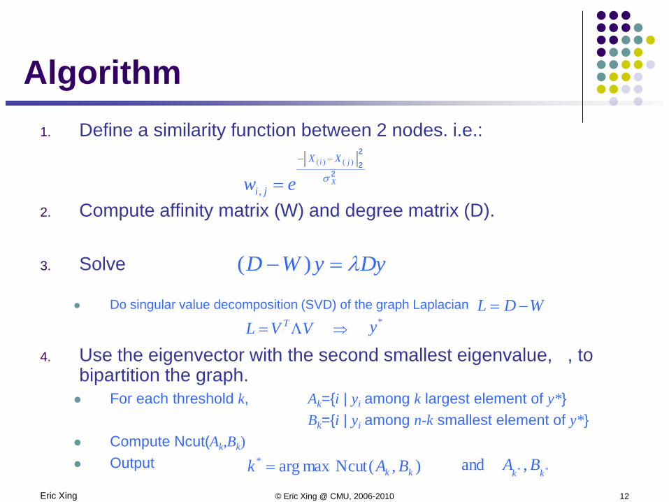
Algorithm1. Define a similarity function between 2 nodes. i.e.:

2. Compute affinity matrix (W) and degree matrix (D).

3. Solve

Do singular value decomposition (SVD) of the graph Laplacian

4. Use the eigenvector with the second smallest eigenvalue, , to bipartition the graph. For each threshold k, Ak={i | yi among k largest element of y*}

Bk={i | yi among n-k smallest element of y*} Compute Ncut(Ak,Bk) Output

DyyWD λ=− )(

2

2

2

X

ji XX

ji ew σ)()(

,

−−

=

WDL −=VVL TΛ= ⇒ *y

),(Ncut maxarg*kk BAk = ** , and kk BA


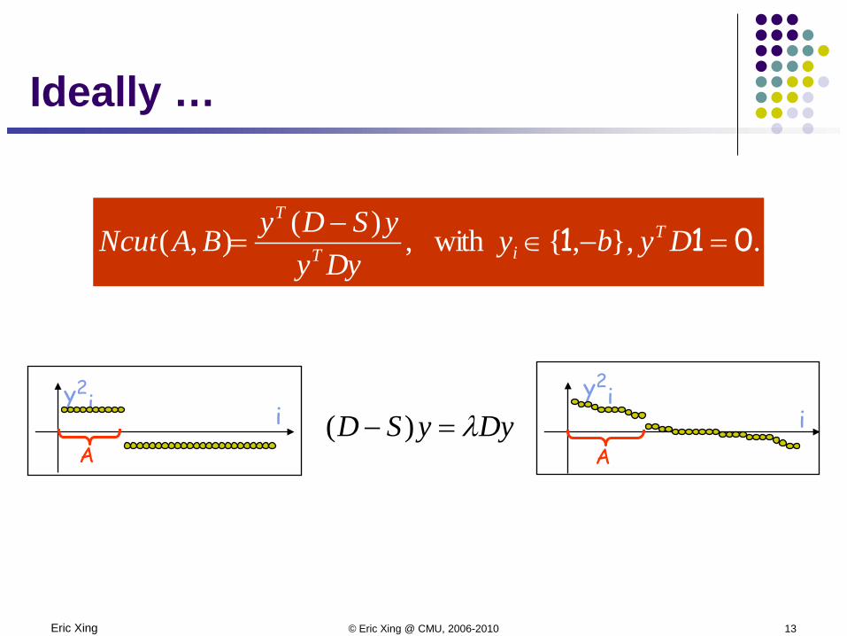
.},,{ with ,)(),( 011 =−∈−

= DybyDyy

ySDyBANcut TiT

T

y2i i

A

y2i

iA

DyySD λ=− )(

Ideally …


Example (Xing et al, 2001)


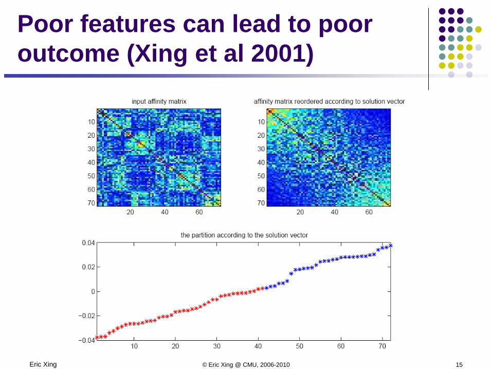
Poor features can lead to poor outcome (Xing et al 2001)


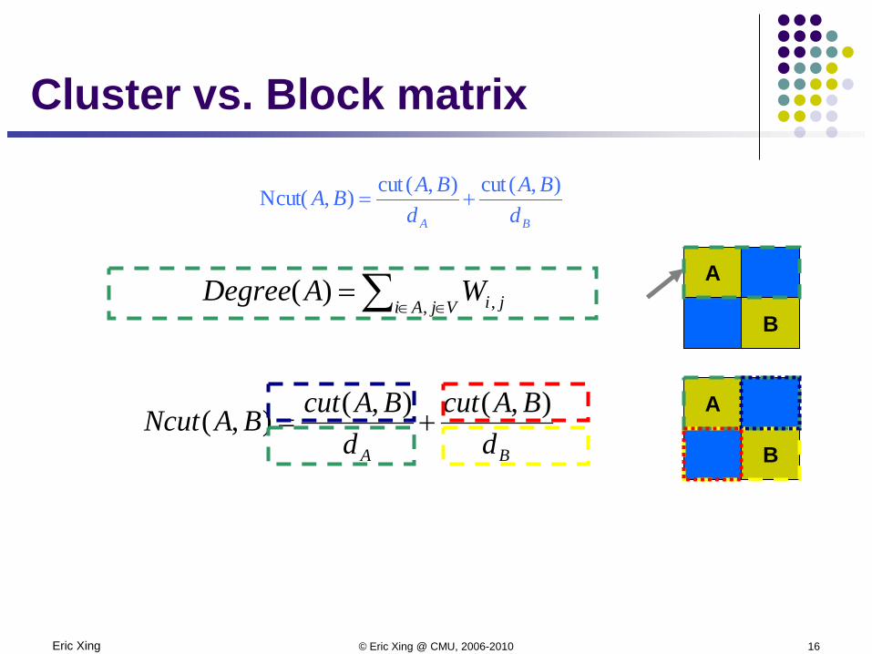
Cluster vs. Block matrix

BA dBAcut

dBAcutBANcut ),(),(),( +=

∑ ∈∈=

VjAi jiWADegree, ,)(

A

B

A

B

BA dBA

dBABA ),(cut),(cut),Ncut( +=


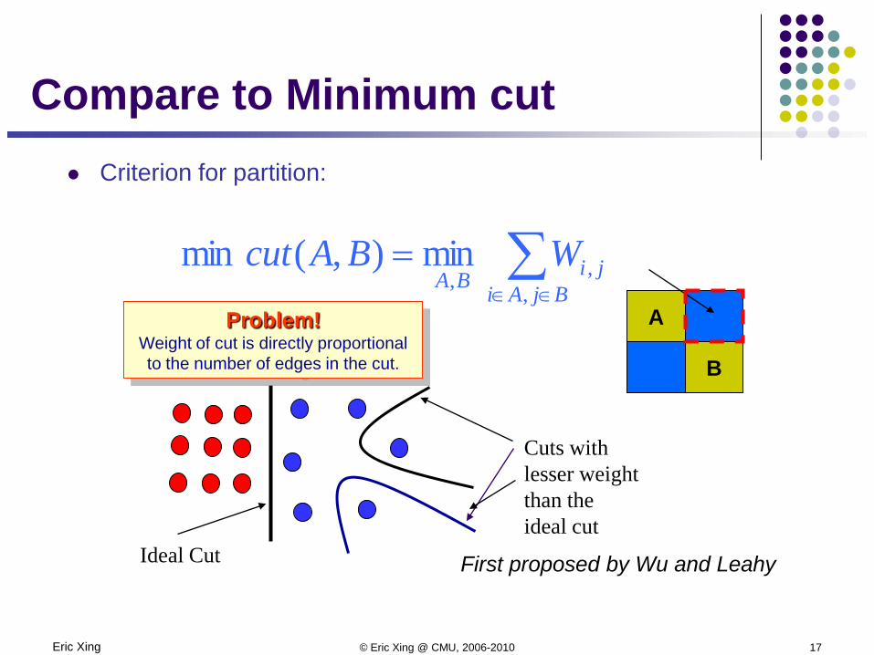
Criterion for partition:

Compare to Minimum cut

∑∈∈

=BjAi

jiBAWBAcut

,,,

min),(min

First proposed by Wu and Leahy

A

B

Ideal Cut

Cuts with lesser weightthan the ideal cut

Problem! Weight of cut is directly proportional to the number of edges in the cut.


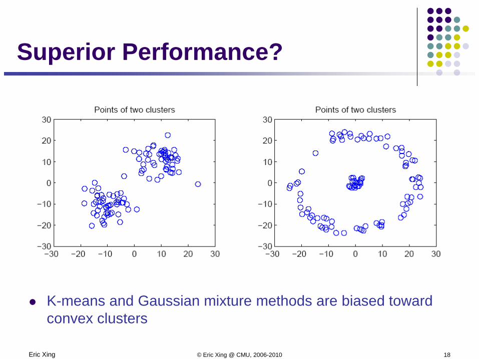
Superior Performance?

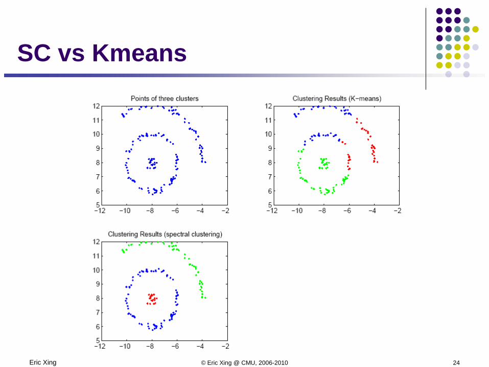
K-means and Gaussian mixture methods are biased toward convex clusters


Ncut is superior in certain cases


Why?


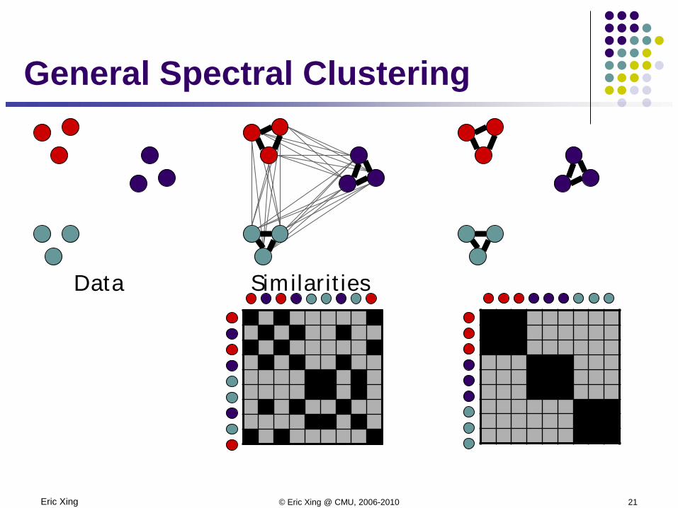
General Spectral Clustering

Data Similarities


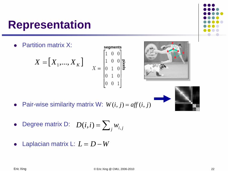
Representation

[ ]KXXX ,...,1=

∑= j jiwiiD ,),(

WDL −=

segments

pixels),(),( jiaffjiW =

Partition matrix X:

Pair-wise similarity matrix W:

Degree matrix D:

Laplacian matrix L:


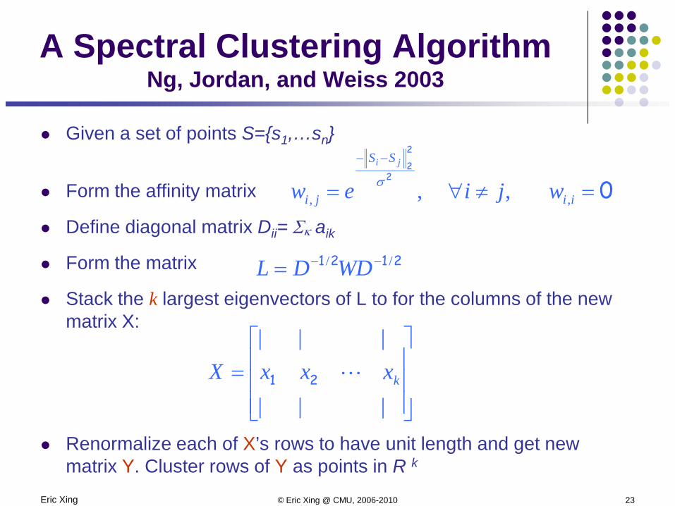
Given a set of points S={s1,…sn}

Form the affinity matrix

Define diagonal matrix Dii= Σκ aik

Form the matrix

Stack the k largest eigenvectors of L to for the columns of the new matrix X:

Renormalize each of X’s rows to have unit length and get new matrix Y. Cluster rows of Y as points in R k

A Spectral Clustering Algorithm Ng, Jordan, and Weiss 2003

02

2

2

=≠∀=

−−

ii

SS

ji wjiewji

,, , ,σ

2121 // −−= WDDL

=

|

|

|

|

|

|

kxxxX 21


SC vs Kmeans


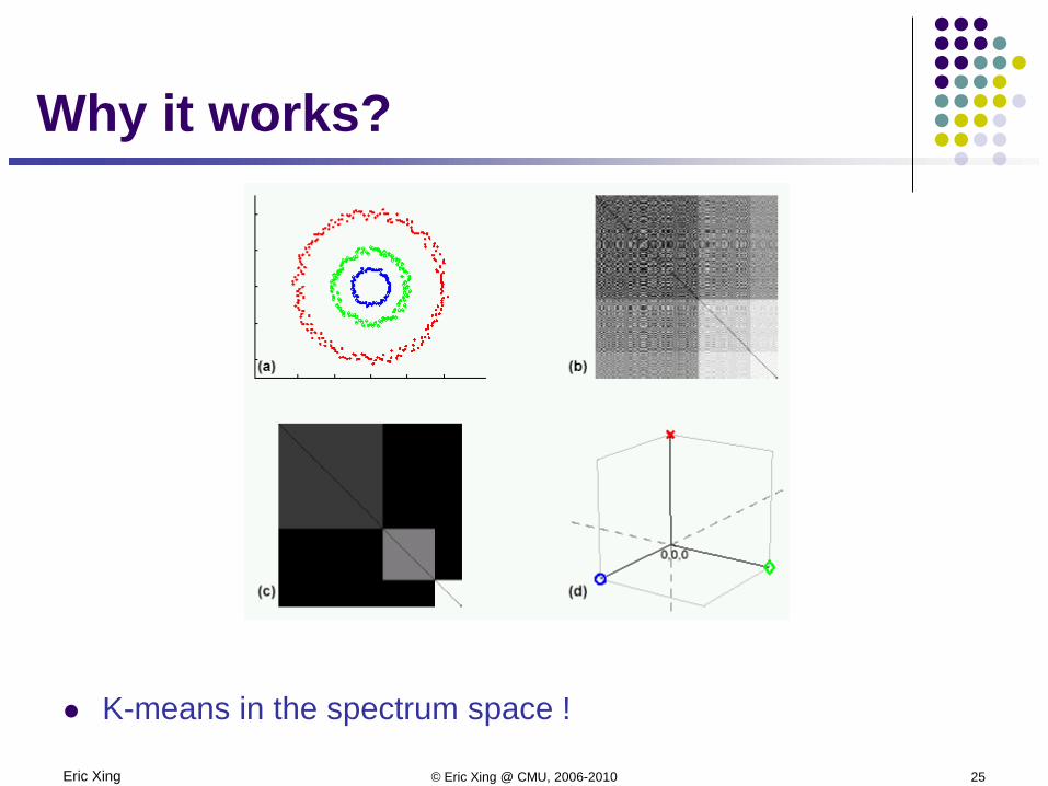
Why it works?

K-means in the spectrum space !


Eigenvectors and blocks

1 1 0 0

1 1 0 0

0 0 1 1

0 0 1 1

eigensolver

.71

.71

0

0

0

0

.71

.71

λ1= 2 λ2= 2 λ3= 0

λ4= 0

1 1 .2 0

1 1 0 -.2

.2 0 1 1

0 -.2 1 1

eigensolver

.71

.69

.14

0

0

-.14

.69

.71

λ1= 2.02 λ2= 2.02 λ3= -0.02

λ4= -0.02

Block matrices have block eigenvectors:

Near-block matrices have near-block eigenvectors:


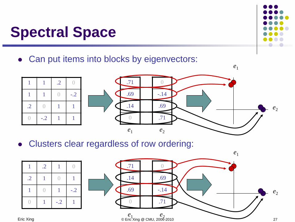
Spectral Space

1 1 .2 0

1 1 0 -.2

.2 0 1 1

0 -.2 1 1

.71

.69

.14

0

0

-.14

.69

.71

e1

e2

e1 e2

1 .2 1 0

.2 1 0 1

1 0 1 -.2

0 1 -.2 1

.71

.14

.69

0

0

.69

-.14

.71

e1

e2

e1 e2

Can put items into blocks by eigenvectors:

Clusters clear regardless of row ordering:


More formally … Recall generalized Ncut

Minimizing this is equivalent to spectral clustering

∑∑ ∑∑

== ∈∈

∈∈

=

=

k

r A

rrk

r VjAi ij

AVjAi ijk

rr

rr

dAA

W

WAAA

1121

),(cut),Ncut(,

\,

∑=

=

k

r A

rrk

rd

AAAAA1

21),(cut),Ncut(min

YWDDY 2121 //Tmin −−

IYY =T s.t.

segments

pixelsY


Spectral Clustering Algorithms that cluster points using eigenvectors of matrices

derived from the data

Obtain data representation in the low-dimensional space that can be easily clustered

Variety of methods that use the eigenvectors differently (we have seen an example)

Empirically very successful

Authors disagree: Which eigenvectors to use How to derive clusters from these eigenvectors

Two general methods


Method #1 Partition using only one eigenvector at a time Use procedure recursively Example: Image Segmentation

Uses 2nd (smallest) eigenvector to define optimal cut Recursively generates two clusters with each cut


Method #2 Use k eigenvectors (k chosen by user)

Directly compute k-way partitioning

Experimentally has been seen to be “better”


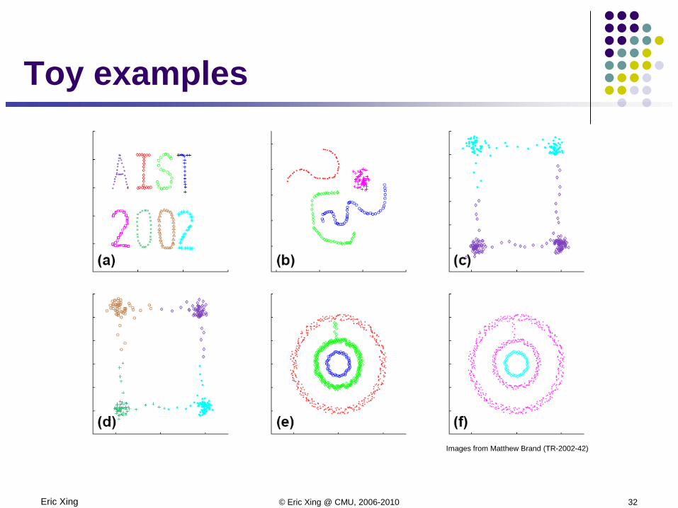
Toy examples

Images from Matthew Brand (TR-2002-42)


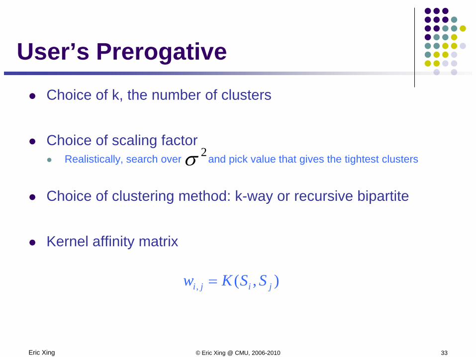
User’s Prerogative Choice of k, the number of clusters

Choice of scaling factor Realistically, search over and pick value that gives the tightest clusters

Choice of clustering method: k-way or recursive bipartite

Kernel affinity matrix

2σ

),(, jiji SSKw =


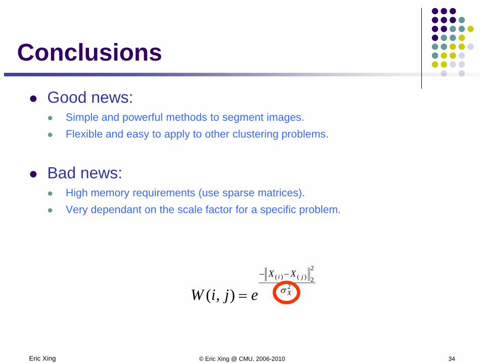
Conclusions

Good news: Simple and powerful methods to segment images. Flexible and easy to apply to other clustering problems.

Bad news: High memory requirements (use sparse matrices). Very dependant on the scale factor for a specific problem.

2

2

2)()(

),( X

ji XX

ejiW σ

−−

=

lecture8 xing

Art & Photos