Lectures 19 & 20: MONETARY DETERMINATION OF EXCHANGE RATES• Building blocs

- Interest rate parity- Money demand equation- Goods markets

• Flexible-price version: monetarist/Lucas model- derivation - applications: hyperinflation; speculative bubbles

• Sticky-price version: Dornbusch overshooting model

• Appendix: Forecasting

Motivations of the monetary approach

Because S is the price of foreign money (vs. domestic money), it is determined by the supply & demand for money (foreign vs. domestic).

Key assumptions:• Perfect capital mobility => speculators are able

to adjust their portfolios quickly to reflect their desires.

• There is no exchange risk premium => UIP holds: esii *

Key results:• S is highly variable, like other asset prices.

• Expectations are central.

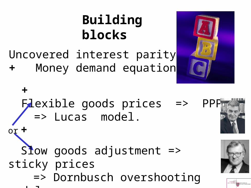
Uncovered interest parity + Money demand equation

+Flexible goods prices => PPP => Lucas model.

Building blocks

or +

Slow goods adjustment => sticky prices=> Dornbusch overshooting

model .

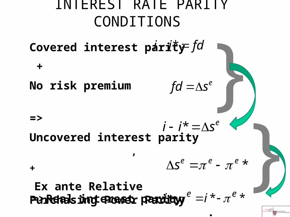
INTEREST RATE PARITY CONDITIONS

Covered interest parity

+

No risk premium

=>

Uncovered interest parity ,+

Ex ante Relative Purchasing Power Parity

fdii *

esfd

esii *

*eees

** ee ii

}=> Real interest parity .

}

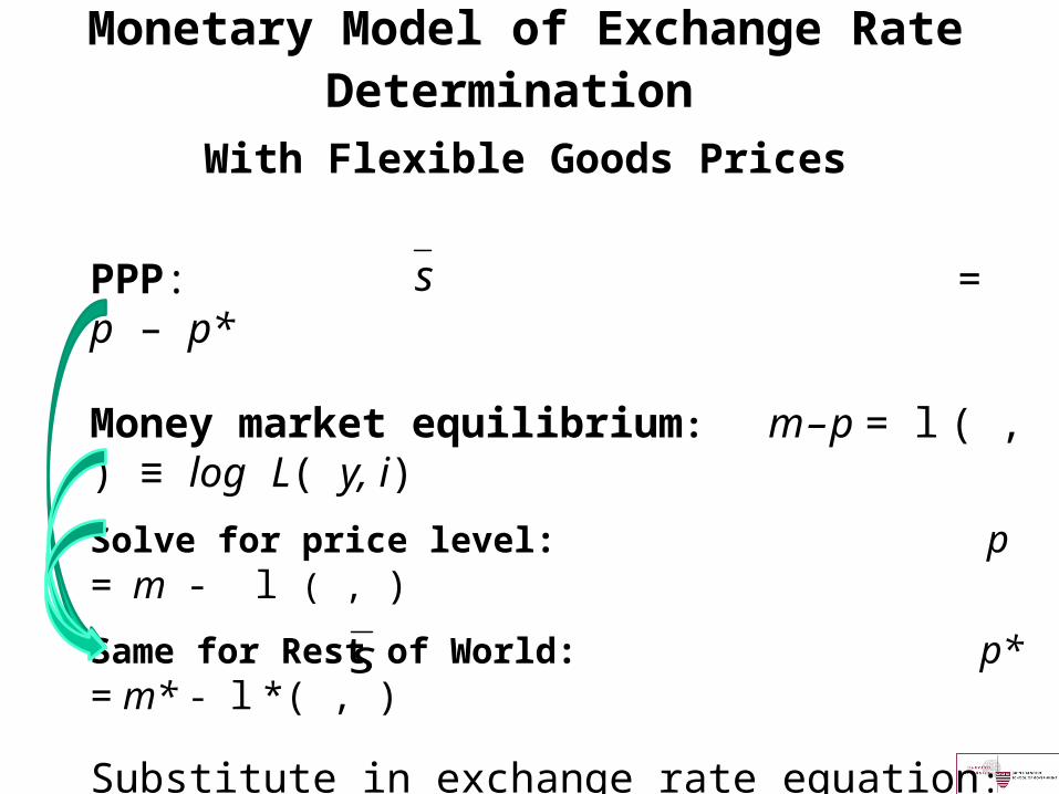
Monetary Model of Exchange Rate Determination

With Flexible Goods Prices

PPP: = p – p*

Money market equilibrium: m – p = l ( , ) ≡ log L( y, i)

Solve for price level: p = m - l ( , )

Same for Rest of World: p* = m* - l *( , )

Substitute in exchange rate equation:

= [m - l ( , )] – [m* - l *( , )]

= [m - m*] – [l ( , ) – l *( , )] .

s

s

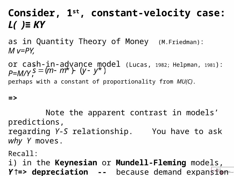
Consider, 1st, constant-velocity case: L( )≡ KY

as in Quantity Theory of Money (M.Friedman): M v=PY,

or cash-in-advance model (Lucas, 1982; Helpman, 1981): P=M/Y,perhaps with a constant of proportionality from MU(C).

=>

Note the apparent contrast in models’ predictions, regarding Y-S relationship. You have to ask why Y moves.

Recall: i) in the Keynesian or Mundell-Fleming models, Y => depreciation -- because demand expansion is assumed the origin, so TB worsens.

But ii) in the flex-price or Lucas model, an increase in Y originates in supply, , and so raises the demand for money => appreciation.

*)(*)( yymms

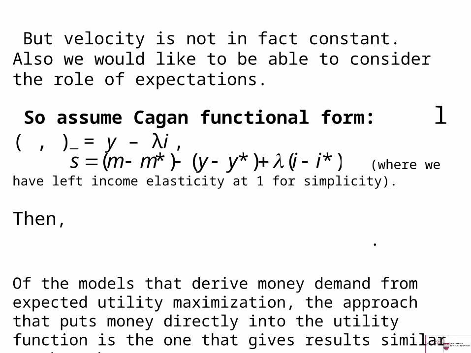
But velocity is not in fact constant. Also we would like to be able to consider the role of expectations.

So assume Cagan functional form: l ( , ) = y – λi , (where we have left income elasticity at 1 for simplicity).

Then, .

Of the models that derive money demand from expected utility maximization, the approach that puts money directly into the utility function is the one that gives results similar to those here. (See Obstfeld-Rogoff, 1996, pp. 579-585.)

A 3rd alternative, the Overlapping Generations model (OLG), is not really a model of demand for money per se (as opposed to bonds).

*)(*)(*)( iiyymms

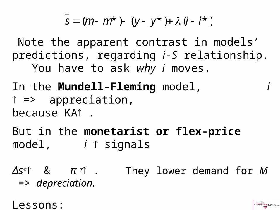
Note the apparent contrast in models’ predictions, regarding i-S relationship. You have to ask why i moves.

In the Mundell-Fleming model, i => appreciation, because KA .

But in the monetarist or flex-price model, i signals Δse & π e . They lower demand for M => depreciation.

Lessons: (i) For predictions regarding relationships among endogenous macro variables, you need to know exogenous source of disturbance.

(ii) Different models are useful in different circumstances.

*)(*)(*)( iiyymms

*)(*)(*)( eeyymms

)(*)(*)( esyymms

)(*)(*)( fdyymms

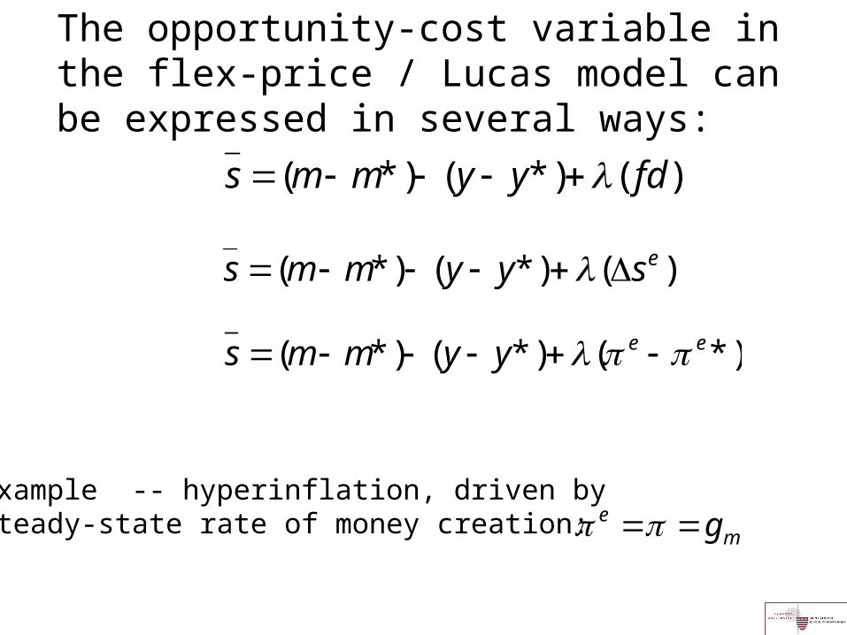
The opportunity-cost variable in the flex-price / Lucas model can be expressed in several ways:

me g

Example -- hyperinflation, driven by steady-state rate of money creation:

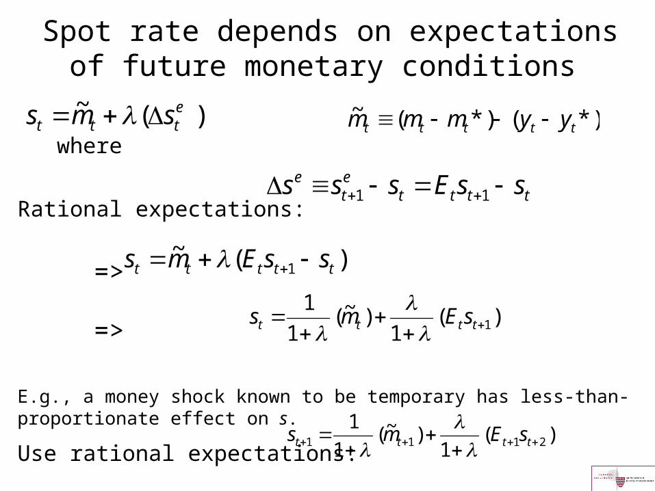
Spot rate depends on expectationsof future monetary conditions

)(~ ettt sms *)(*)(~

ttttt yymmm where

Rational expectations:

=>

=>

E.g., a money shock known to be temporary has less-than-proportionate effect on s.

Use rational expectations:

ttttet

e ssEsss 11

)(~1 ttttt ssEms

)(1

)~(1

11

tttt sEms

)(1

)~(1

12111

tttt sEms

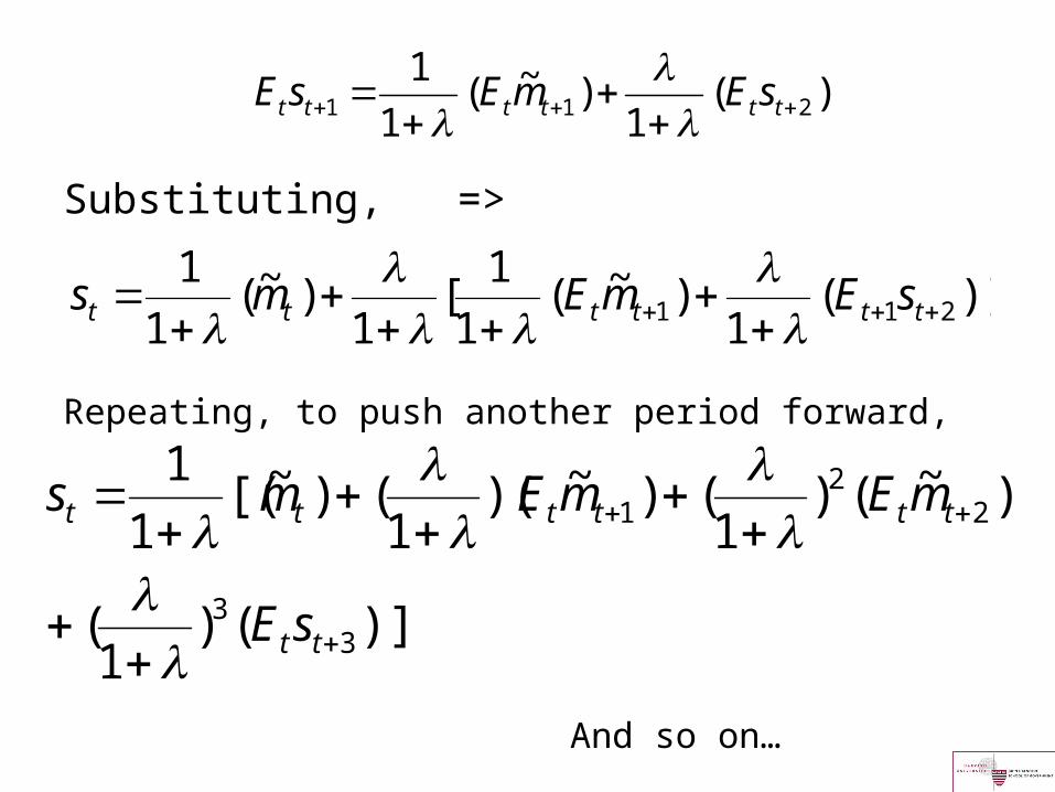
Substituting, =>

Repeating, to push another period forward,

And so on…

)(1

)~(1

1211

tttttt sEmEsE

)](1

)~(1

1[

1)~(

1

1211

tttttt sEmEms

)]()1(

)]~()1()~)(

1()~[(

1

1

33

22

1

tt

tttttt

sE

mEmEms

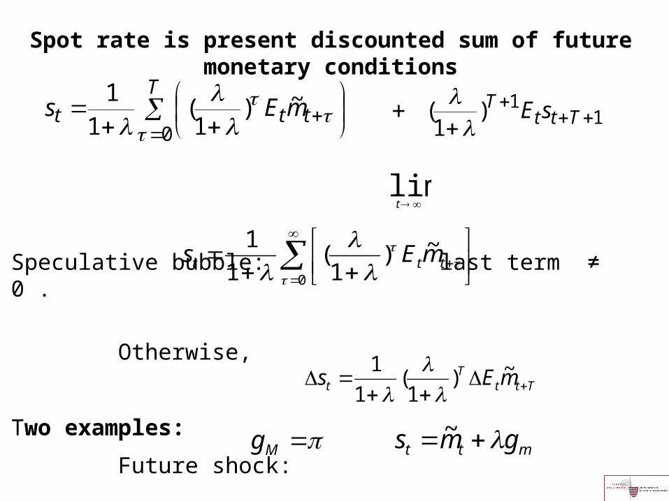
Spot rate is present discounted sum of future monetary conditions

Speculative bubble: last term ≠ 0 .

Otherwise,

Two examples:

Future shock:

Trend money growth :

0

~)1(

1

1

ttt mEs

TttT

t mEs

~)1(

1

1

Mg mtt gms ~

T

ttt mEs0

~)1(

11

1

1)1(

Ttt

T sE

+

limt

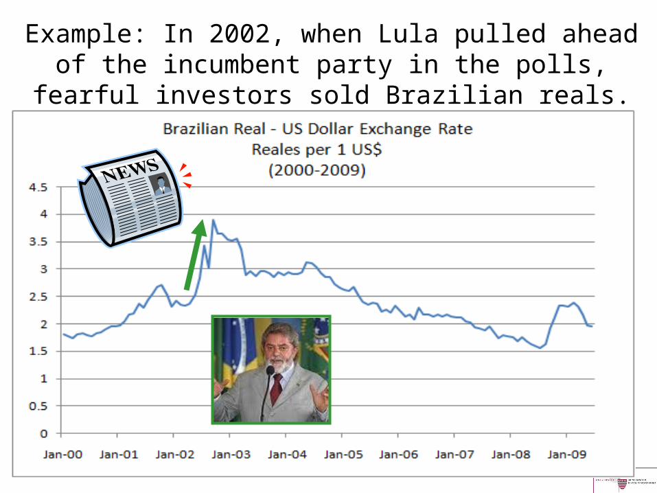
Example: In 2002, when Lula pulled ahead of the incumbent party in the polls, fearful investors sold Brazilian reals.

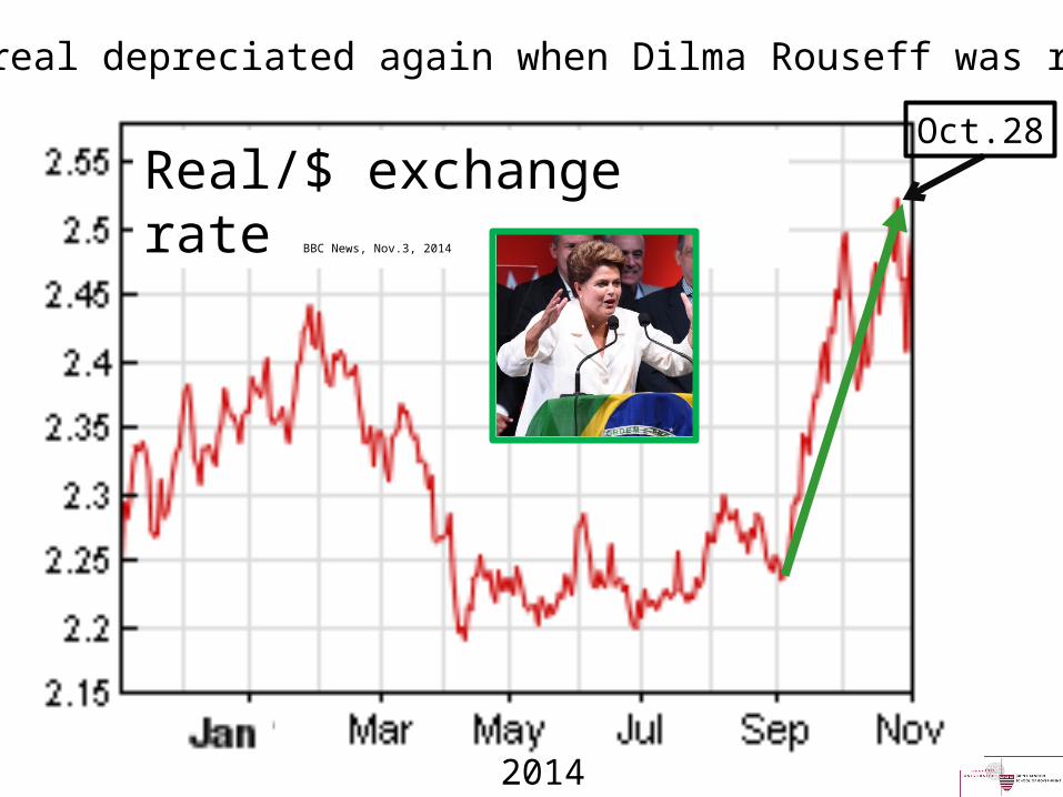
Real/$ exchange rate BBC News, Nov.3, 2014

2014

Oct.28

Brazil’s real depreciated again when Dilma Rouseff was reelected.

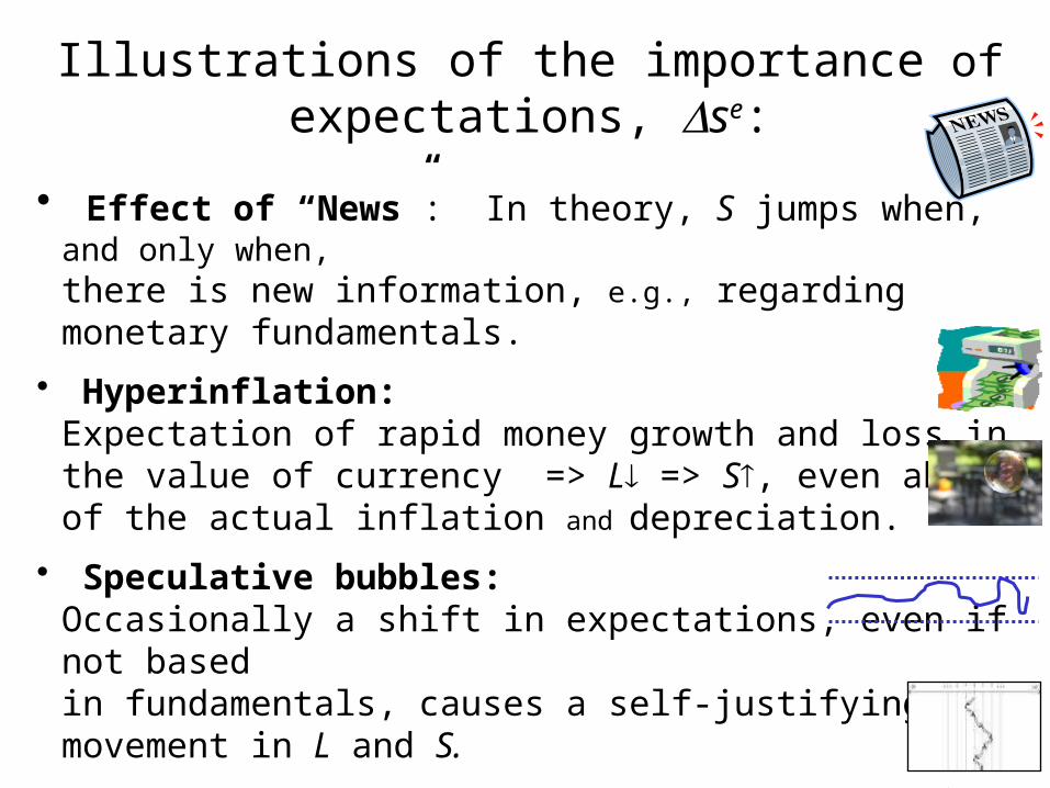
Illustrations of the importance of expectations, se:

• Effect of “News”: In theory, S jumps when, and only when, there is new information, e.g., regarding monetary fundamentals.

• Hyperinflation: Expectation of rapid money growth and loss in the value of currency => L => S, even ahead of the actual inflation and

depreciation.

• Speculative bubbles: Occasionally a shift in expectations, even if not based in fundamentals, causes a self-justifying movement in L and S.

• Target zone: If a band is credible, speculation can stabilize S -- pushing it away from the edges even before intervention.

• “Random walk”: Today’s price already incorporates information about the future (but RE does not imply the zero forecastability of a RW)

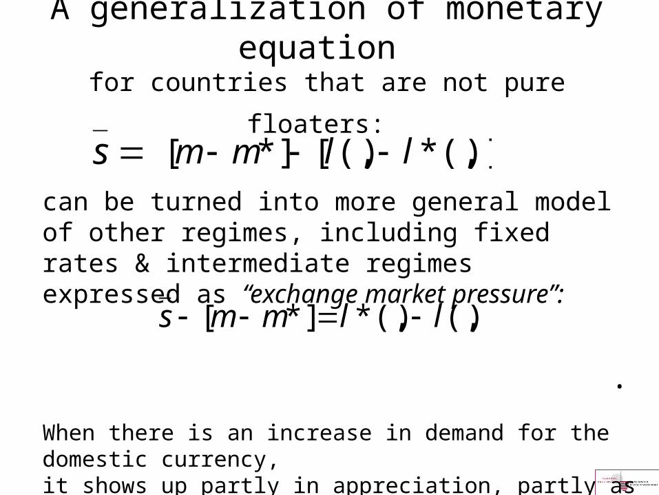
A generalization of monetary equation for countries that are not pure floaters:

can be turned into more general model of other regimes, including fixed rates & intermediate regimesexpressed as “exchange market pressure”:

.

When there is an increase in demand for the domestic currency, it shows up partly in appreciation, partly as increase in reserves & money supply, with the split determined by the central bank.

)(,)(,**][ llmms

)](,*)(,[*][ llmm s

Limitations of the monetarist/Lucas modelof exchange rate determination

No allowance for SR variation in:

the real exchange rate Q

the real interest rate r .

One approach: International versions of Real Business Cycle models assume all observed variation in Q is due to variation in LR equilibrium (and r is due to ), in turn due to shifts in tastes or productivity.

But we want to be able to talk about transitory deviations of Q from (and r from ), arising for monetary reasons.

=> Dornbusch overshooting model.

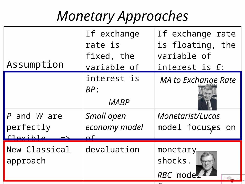
Monetary Approaches

Assumption

If exchange rate is fixed, the variable of interest is BP:

MABP

If exchange rate is floating, the variable of interest is E:

MA to Exchange Rate

P and W are perfectly flexible => New Classical approach

Small open economy model of devaluation

Monetarist/Lucas model focuses on monetary shocks.RBC model focuses on supply shocks ( ).

P is sticky Mundell-Fleming

(fixed rates)

Dornbusch-Mundell-Fleming (floating)

Y