Lectures on analytic torsion

Ulrich Bunke∗

July 14, 2015

Abstract

Contents

1 Analytic torsion - from algebra to analysis - the finite-dimensional case 21.1 Torsion of chain complexes . . . . . . . . . . . . . . . . . . . . . . . . . . . 21.2 Torsion and Laplace operators . . . . . . . . . . . . . . . . . . . . . . . . . 41.3 Torsion and Whitehead torsion . . . . . . . . . . . . . . . . . . . . . . . . 7

2 Zeta regularized determinants of operators - Ray-Singer torsion 92.1 Motivation . . . . . . . . . . . . . . . . . . . . . . . . . . . . . . . . . . . . 92.2 Spectral zeta functions . . . . . . . . . . . . . . . . . . . . . . . . . . . . . 102.3 Analytic torsion . . . . . . . . . . . . . . . . . . . . . . . . . . . . . . . . . 142.4 Ray-Singer torsion . . . . . . . . . . . . . . . . . . . . . . . . . . . . . . . 152.5 Torsion for flat bundles on the circle . . . . . . . . . . . . . . . . . . . . . 17

3 Morse theory, Witten deformation, and the Muller-Cheeger theorem 203.1 Morse theory . . . . . . . . . . . . . . . . . . . . . . . . . . . . . . . . . . 203.2 The Morse-Smale complex . . . . . . . . . . . . . . . . . . . . . . . . . . . 223.3 Milnor metric and Ray-Singer metric . . . . . . . . . . . . . . . . . . . . . 24

4 The Witten deformation 264.1 The Witten deformation . . . . . . . . . . . . . . . . . . . . . . . . . . . . 264.2 A model case . . . . . . . . . . . . . . . . . . . . . . . . . . . . . . . . . . 284.3 The spectrum of the Witten Laplacian . . . . . . . . . . . . . . . . . . . . 304.4 The small eigenvalue complex . . . . . . . . . . . . . . . . . . . . . . . . . 32

∗NWF I - Mathematik, Universitat Regensburg, 93040 Regensburg, GERMANY,ulrich.bunke@mathematik.uni-regensburg.de

1

1 Analytic torsion - from algebra to analysis - the

finite-dimensional case

1.1 Torsion of chain complexes

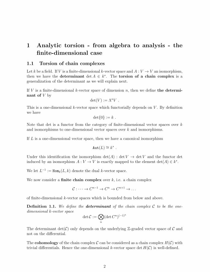
Let k be a field. If V is a finite-dimensional k-vector space and A : V → V an isomorphism,then we have the determinant detA ∈ k∗. The torsion of a chain complex is ageneralization of the determinant as we will explain next.

If V is a finite-dimensional k-vector space of dimension n, then we define the determi-nant of V by

det(V ) := ΛnV .

This is a one-dimensional k-vector space which functorially depends on V . By definitionwe have

det0 := k .

Note that det is a functor from the category of finite-dimensional vector spaces over kand isomorphisms to one-dimensional vector spaces over k and isomorphisms.

If L is a one-dimensional vector space, then we have a canonical isomorphism

Aut(L) ∼= k∗ .

Under this identification the isomorphism det(A) : detV → detV and the functor detinduced by an isomorphism A : V → V is exactly mapped to the element det(A) ∈ k∗.

We let L−1 := Homk(L, k) denote the dual k-vector space.

We now consider a finite chain complex over k, i.e. a chain complex

C : · · · → Cn−1 → Cn → Cn+1 → . . .

of finite-dimensional k-vector spaces which is bounded from below and above.

Definition 1.1. We define the determinant of the chain complex C to be the one-dimensional k-vector space

det C :=⊗n

(detCn)(−1)n

The determinant det(C) only depends on the underlying Z-graded vector space of C andnot on the differential.

The cohomology of the chain complex C can be considered as a chain complex H(C) withtrivial differentials. Hence the one-dimensional k-vector space detH(C) is well-defined.

2

Proposition 1.2. We have a canonical isomorphism

τC : det C∼=→ detH(C) .

This isomorphism is called the torsion isomorphism.

Proof. For two finite-dimensional k-vector spaces U,W we have a canonical isomorphism

det(U ⊕W ) ∼= detU ⊗ detW .

More generally, given a short exact sequence (with U in degree 0)

V : 0→ U → V → W → 0

we can choose a split. It induces a decomposition V ∼= U ⊕W and therefore an isomor-phism

detU ⊗ detW ∼= detV .

The main observation is that this isomorphism does not depend on the choice of the split.The torsion of the short exact sequence V is the induced isomorphism

τV : detU ⊗ (detV )−1 ⊗ detW → k .

Finally, we can decompose a chain complex C into short exact sequences and construct thetorsion inductively by the length of the chain complex. Assume that C starts at n ∈ Z.We consider the two short exact sequences

A : 0→ Hn(C)→ Cn → Bn+1 → 0 ,

B : 0→ Bn+1 → Cn+1 → Cn+1/Bn+1 → 0 ,

and the sequenceC ′ : 0→ Cn+1/Bn+1 → Cn+2 → · · · → .

Here Bn+1 := d(Cn) ⊂ Cn+1 denotes the subspace of boundaries. Note that C ′ starts indegree n+ 1. By induction, the isomorphism τC is defined by

det(C) ∼= (detCn)(−1)n ⊗ (detCn+1)(−1)n+1 ⊗∞⊗

k=n+2

(detCk)(−1)k

τA∼= (detHn(C))(−1)n ⊗ (detBn+1)(−1)n ⊗ (detCn+1)(−1)n+1 ⊗∞⊗

k=n+2

(detCk)(−1)k

τB∼= (detHn(C))(−1)n ⊗ (det(Cn+1/Bn+1))(−1)n+1 ⊗∞⊗

k=n+2

(detCk)(−1)k

∼= (detHn(C))(−1)n ⊗ det C ′τC′∼= (detHn(C))(−1)n ⊗ detH(C ′)∼= detH(C) .

2

3

Example 1.3. If A : V → W is an isomorphism of finite-dimensional vector spaces, thenwe can form the acyclic complex

A : V → W

with W in degree 0. Its torsion is an isomorphism

τA : (detV )−1 ⊗ detW → k∗

which corresponds to the generalization of the determinant of A as a morphism det(A) :detV → detW . Only for V = W we can interpret this as an element in k∗.

Example 1.4. Let C be a finite chain complex and W be a finite-dimensional k-vectorspace. Then we form the chain complex

W : WidW→ W

starting at 0 and let n ∈ Z. We say that the chain complex C ′ := C ⊕W [n] is obtainedfrom C by a simple expansion.

If C ′ is obtained from C by a simple expansion, then we have canonical isomorphismsdet C ∼= det C ′ and H(C) ∼= H(C ′). Under these isomorphisms we have the equality oftorsion isomorphisms τC = τC′ .

1.2 Torsion and Laplace operators

We now assume that k = R or k = C.

A metric hV on V is a (hermitean in the case k = C) scalar product on V . It inducesa metric hdetV on detV . This metric is fixed by the following property. Let (vi)i=1,...,n

be an orthonormal basis of V with respect to hV , then v1 ∧ · · · ∧ vn is a normalized basisvector of detV with respect to hdetV .

Example 1.5. Let (V, hV ) and (W,hW ) be finite-dimensional k-vector spaces with metricsand A : V → W be an isomorphism of k-vector spaces. Then we can choose an isometryU : W → V . We have the number det(UA) ∈ k∗ which depends on the choice of U . Wenow observe that

| detA| := | det(UA)| ∈ R+ (1)

does not depend on the choice of U . The analytic torsion generalizes this idea to chaincomplexes.

A metric hC on a chain complex is a collection of metrics (hCn)n. Such a metric inducesa metric on det C and therefore, by push-forward, a metric τC,∗h

C on detH(C).

4

Definition 1.6. Let C be a finite chain complex and hC and hH(C) metrics on C and itscohomology H(C). Then the analytic torsion

T (C, hC, hH(C)) ∈ R+

is defined by the relation

hdetH(C) = T (C, hC, hH(C)) τC,∗hdet C .

Example 1.7. In general the analytic torsion depends non-trivially on the choice ofmetrics. For example, if t, s ∈ R+, then we have the relation

T (C, shC, thH(C)) = (t

s)χ(C) ,

where χ(C) ∈ Z denotes the Euler characteristic of C. But observe that if C is acyclic,then χ(C) = 0 and T (C, hC, hH(C)) does not depend on the scale of the metrics.

Example 1.8. In this example we discuss the dependence of the analytic torsion on thechoice of hH(C). Assume that h

H(C)i , i = 0, 1 are two choices. Then we define numbers

vk(hH(C)0 , h

H(C)1 ) ∈ R+ uniquely such that

vk(hH(C)0 , h

H(C)1 ) h

detHk(C)1 = h

detHk(C)0 .

We further setv(h

H(C)0 , h

H(C)1 ) :=

∏k

vk(hH(C)0 , h

H(C)1 )(−1)k .

Then we haveT (C, hC, hH(C)

0 ) = v(hH(C)0 , h

H(C)1 ) T (C, hC, hH(C)

1 ) .

We consider the Z-graded vector space

C :=⊕n∈Z

Cn

and the differential d : C → C as a linear map of degree one. The metric hC induces ametric hC such that the graded components are orthogonal. Using hC we can define theadjoint d∗ : C → C which has degree −1. We define the Laplace operator

∆ := (d+ d∗)2 .

Since d2 = 0 and (d∗)2 = 0 we have ∆ = dd∗+ d∗d. Hence the Laplace operator preservesdegree and therefore decomposes as

∆ = ⊕n∈Z∆n .

5

As in Hodge theory we have an orthogonal decomposition

C ∼= im(d)⊕ ker∆⊕ im(d∗) , ker(d) = im(d)⊕ ker∆ .

In particular, we get an isomorphism isomorphism of graded vector spaces

H(C) ∼= ker(∆) .

This isomorphism induces the Hodge metric hH(C)Hodge on H(C).

We let ∆′n be the restriction of ∆n to the orthogonal complement of ker(∆n).

Lemma 1.9. We have the equality

T (C, hC, hH(C)Hodge) =

√∏n∈Z

det(∆′n)(−1)nn .

Proof. The differential d induces an isomorphism of vector space

dk : Ck ⊇ ker(d|Ck)⊥ ∼= im(d|Ck) ⊆ Ck+1 .

First show inductively that∏k

| det dk|(−1)k+1

τC : det C → detH(C)

is an isometry (see (1) for notation), hence

T (C, hC, hH(C)Hodge) =

[∏k

| det dk|(−1)k+1

]. (2)

We repeat the construction of the torsion isomorphism. But in addition we introducefactors to turn each step into an isometry. Note that

| det(dk)|−1 det(dk) : det(ker(d|Ck)⊥)→ det(im(d|Ck))

is an isometry. This accounts for the first correction factor in the following chain of

6

isometries.

det(C) ∼= (detCn)(−1)n ⊗ (detCn+1)(−1)n+1∞⊗

k=n+2

(detCk)(−1)k

|det dn|(−1)n+1τA→ (detHn(C))(−1)n ⊗ (detBn+1)(−1)n ⊗ (detCn+1)(−1)n+1 ⊗

∞⊗k=n+2

(detCk)(−1)k

τB∼= (detHn(C))(−1)n ⊗ (det(Cn+1/Bn+1))(−1)n+1 ⊗∞⊗

k=n+2

(detCk)(−1)k

∼= (detHn(C))(−1)n ⊗ det(C ′)∏∞k=n+1 | det dk|(−1)k+1

τC′∼= (detHn(C))(−1)n ⊗ detH(C ′)

∼=∞∏

k=n+1

detH(C) .

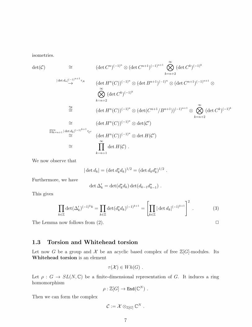
We now observe that

| det dk| = (det d∗kdk)1/2 = (det dkd

∗k)

1/2 .

Furthermore, we havedet ∆′k = det(d∗kdk) det(dk−1d

∗k−1) .

This gives

∏k∈Z

det(∆′k)(−1)kk =

∏k∈Z

det(d∗kdk)(−1)k+1

=

[∏k∈Z

| det dk|(−1)k+1

]2

. (3)

The Lemma now follows from (2). 2

1.3 Torsion and Whitehead torsion

Let now G be a group and X be an acyclic based complex of free Z[G]-modules. ItsWhitehead torsion is an element

τ(X ) ∈ Wh(G) .

Let ρ : G → SL(N,C) be a finite-dimensional representation of G. It induces a ringhomomorphism

ρ : Z[G]→ End(CN) .

Then we can form the complex

C := X ⊗Z[G] CN .

7

Lemma 1.10. This complex is acyclic.

Proof. The acyclic complex of free (or more generally, of projective) Z[G]-modules X ad-mits a chain contraction. We get an induced chain contraction of C. 2

The basis of X together with the standard orthonormal basis of CN induces a basis of Cwhich we declare to be orthonormal, thus defining a metric hC. Since H(C) = 0 we have acanonical metric hH(C) on H(C) = C and the analytic torsion T (C, hC) := T (C, hC, hH(C))is defined.

The representation ρ induces a homomorphism

K1(Z[G])→ K1(End(CN)) ∼= K1(C) ∼= C∗ ‖.‖→ R+ .

Under this homomorphism

K1(Z[G]) 3 [±g] 7→ | det(±ρ(g))| = 1 ∈ R+ .

Therefore, by passing through the quotient, we get a well-defined homomorphism

χρ: : Wh(G) = K1(Z[G])/(±[g])→ R+ . (4)

Proposition 1.11. The Whitehead torsion and the analytic torsion are related by

T (C, hC) = χρ(τ(X )) .

Proof. We can define the Whitehead torsion of based complexes X over Z[G] again in-ductively by the length. We make the simplifying assumption that the complements ofthe images of the differentials are free. Assume that the complex X starts with Xn. Weconsider the short exact sequence of Z[G]-modules

0→ Xn → Xn+1p→ Xn+1/Xn → 0

and setX ′ : 0→ Xn+1/Xn

i→ Xn+2 → . . . .

Let cn be the chosen basis of Xn. We choose a basis c′n+1 of Xn+1/Xn. Lifting its elementsand combining it with the images of the elements of cn and get a basis b′ of Xn+1. Notethat X ′ is again based (by c′k := ck for k ≥ n + 2 and the basis c′n+1 chosen above) andstarts at n+ 1. Then by definition of the Whitehead torsion

τ(X ) = [cn+1/b′](−1)n+1

τ(X ′) ∈ Wh(G) .

Note thatT (C, hC) = T (D, hD) T (C ′, hC′) ,

whereD : 0→ Xn ⊗Z[G] CN → Xn+1 ⊗Z[G] CN p→ Xn+1/Xn ⊗Z[G] CN → 0

8

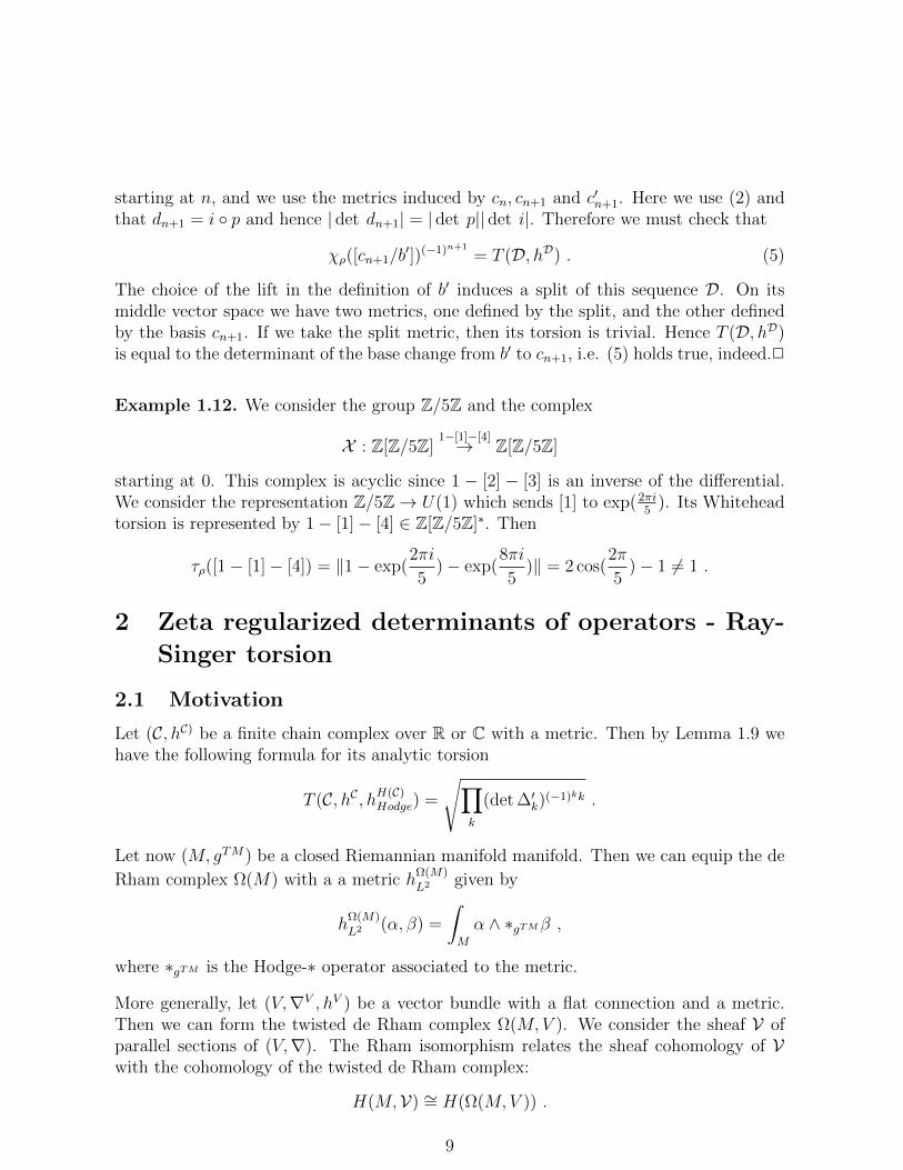
starting at n, and we use the metrics induced by cn, cn+1 and c′n+1. Here we use (2) andthat dn+1 = i p and hence | det dn+1| = | det p|| det i|. Therefore we must check that

χρ([cn+1/b′])(−1)n+1

= T (D, hD) . (5)

The choice of the lift in the definition of b′ induces a split of this sequence D. On itsmiddle vector space we have two metrics, one defined by the split, and the other definedby the basis cn+1. If we take the split metric, then its torsion is trivial. Hence T (D, hD)is equal to the determinant of the base change from b′ to cn+1, i.e. (5) holds true, indeed.2

Example 1.12. We consider the group Z/5Z and the complex

X : Z[Z/5Z]1−[1]−[4]→ Z[Z/5Z]

starting at 0. This complex is acyclic since 1 − [2] − [3] is an inverse of the differential.We consider the representation Z/5Z→ U(1) which sends [1] to exp(2πi

5). Its Whitehead

torsion is represented by 1− [1]− [4] ∈ Z[Z/5Z]∗. Then

τρ([1− [1]− [4]) = ‖1− exp(2πi

5)− exp(

8πi

5)‖ = 2 cos(

2π

5)− 1 6= 1 .

2 Zeta regularized determinants of operators - Ray-

Singer torsion

2.1 Motivation

Let (C, hC) be a finite chain complex over R or C with a metric. Then by Lemma 1.9 wehave the following formula for its analytic torsion

T (C, hC, hH(C)Hodge) =

√∏k

(det ∆′k)(−1)kk .

Let now (M, gTM) be a closed Riemannian manifold manifold. Then we can equip the de

Rham complex Ω(M) with a a metric hΩ(M)

L2 given by

hΩ(M)

L2 (α, β) =

∫M

α ∧ ∗gTMβ ,

where ∗gTM is the Hodge-∗ operator associated to the metric.

More generally, let (V,∇V , hV ) be a vector bundle with a flat connection and a metric.Then we can form the twisted de Rham complex Ω(M,V ). We consider the sheaf V ofparallel sections of (V,∇). The Rham isomorphism relates the sheaf cohomology of Vwith the cohomology of the twisted de Rham complex:

H(M,V) ∼= H(Ω(M,V )) .

9

The metric hV together with the Riemannian metric gTM induce a metric hΩ(M,V )

L2 on thetwisted de Rham complex.

Note that to give (V,∇) is, up to isomorphism, equivalent to give a representation of thefundamental group

π1(M)→ End(Cdim(V ))

(we assume M to be connected, for simplicity). Hence (M,V,∇V ) is differential-topological data, while the metrics gTM and hV are additional geometric choices.

In this section we discuss the definition of analytic torsion

T (M,∇V , gTM , hV ) :=

√∏k

(det ∆′k)(−1)kk

which is essentially due to Ray-Singer [RS71]. To this end we must define the determinantof the Laplace operators properly. We will also discuss in detail, how the torsion dependson the metrics.

2.2 Spectral zeta functions

We consider a finite-dimensional vector space with metric (V, hV ) and a linear, invertible,selfadjoint and positive map ∆ : V → V . Then the endomorphism log(∆) is defined byspectral theory and we have the relation

eTr log ∆ = det(∆) .

The spectral zeta function of ∆ is defined by

ζ∆(s) = Tr ∆−s , s ∈ C .

It is an entire function on C and satisfies

−ζ ′∆(0) = Tr log(∆) .

So we get the formula for the determinant of ∆ in terms of the spectral zeta function

det ∆ = e−ζ′∆(0) .

The idea is to use this formula to define the determinant in the case where ∆ is a differ-ential operator.

We now consider a closed Riemannian manifold (M, gTM) and a vector bundle (V,∇V , hV )with connection and metric. The metrics induce L2-scalar products on Ωk(M,V ) so thatwe can form the adjoint

∇V,∗ : Ω1(M,V )→ Ω0(M,V )

10

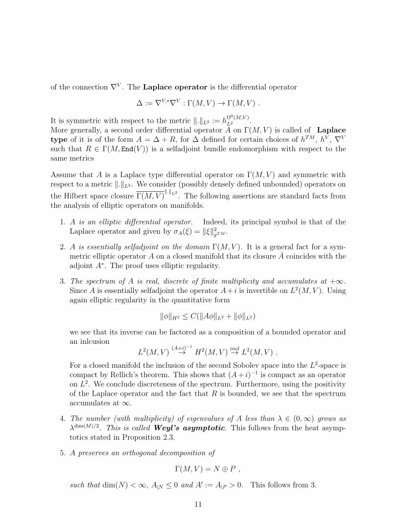
of the connection ∇V . The Laplace operator is the differential operator

∆ := ∇V,∗∇V : Γ(M,V )→ Γ(M,V ) .

It is symmetric with respect to the metric ‖.‖L2 := hΩ0(M,V )

L2 .More generally, a second order differential operator A on Γ(M,V ) is called of Laplacetype of it is of the form A = ∆ + R, for ∆ defined for certain choices of hTM , hV , ∇V

such that R ∈ Γ(M, End(V )) is a selfadjoint bundle endomorphism with respect to thesame metrics

Assume that A is a Laplace type differential operator on Γ(M,V ) and symmetric withrespect to a metric ‖.‖L2 . We consider (possibly densely defined unbounded) operators on

the Hilbert space closure Γ(M,V )‖.‖L2

. The following assertions are standard facts fromthe analysis of elliptic operators on manifolds.

1. A is an elliptic differential operator. Indeed, its principal symbol is that of theLaplace operator and given by σA(ξ) = ‖ξ‖2

gTM .

2. A is essentially selfadjoint on the domain Γ(M,V ). It is a general fact for a sym-metric elliptic operator A on a closed manifold that its closure A coincides with theadjoint A∗. The proof uses elliptic regularity.

3. The spectrum of A is real, discrete of finite multiplicity and accumulates at +∞.Since A is essentially selfadjoint the operator A+ i is invertible on L2(M,V ). Usingagain elliptic regularity in the quantitative form

‖φ‖H2 ≤ C(‖Aφ‖L2 + ‖φ‖L2)

we see that its inverse can be factored as a composition of a bounded operator andan inlcusion

L2(M,V )(A+i)−1

→ H2(M,V )incl→ L2(M,V ) .

For a closed manifold the inclusion of the second Sobolev space into the L2-space iscompact by Rellich’s theorem. This shows that (A+ i)−1 is compact as an operatoron L2. We conclude discreteness of the spectrum. Furthermore, using the positivityof the Laplace operator and the fact that R is bounded, we see that the spectrumaccumulates at ∞.

4. The number (with multiplicity) of eigenvalues of A less than λ ∈ (0,∞) grows asλdim(M)/2. This is called Weyl’s asymptotic. This follows from the heat asymp-totics stated in Proposition 2.3.

5. A preserves an orthogonal decomposition of

Γ(M,V ) = N ⊕ P ,

such that dim(N) <∞, A|N ≤ 0 and A′ := A|P > 0. This follows from 3.

11

6. ζA′(s) := Tr A′,−s is holomorphic for Re(s) > dim(M)/2. This is a consequence ofWeyl’s asymptotic stated in 4.

In order to define ζ ′A(0) we need an analytic continuation of the zeta function. Notethat for λ > 0 and s > 0 we have the equality

λ−s =1

Γ(s)

∫ ∞0

e−tλts−1dt . (6)

We define the Mellin transform of a measurable function θ of t ∈ (0,∞)→ C for s ∈ Cby

M(θ)(s) :=

∫ ∞0

θ(t)ts−1dt ,

provided the integral converges.

Example 2.1. For λ ∈ (0,∞) we have M(eλt)(s) = Γ(s)λ−s.

Lemma 2.2. Assume that θ is exponentially decreasing for t → ∞, and that it has anasymptotic expansion

θ(t)t→0∼

∑n∈N

antαn

for a monotoneously increasing, unbounded sequence (αn)n∈N in R. Then M(θ)(s) isdefined for Re(s) > −α0 and has a meromorphic continuation to all of C with first orderpoles at the points s = −αn, n ∈ N, such that

ress=−αnM(θ)(s) = an .

Proof. This is an exercise. The idea is to split the integral in the Mellin transformationas∫ 1

0+∫∞

1. The second summand yields an entire function. In order to study the first

summand one decomposes θ(t) as a sum of the first n terms of its expansion and a re-mainder. The integral of the asymptotic expansion term can be evaluated explicitly andcontributes the singularities for Re(s) > −αn+1, and the remainder gives a holomorphicfunction on this domain. Since we can choose n arbitrary large we get the assertion. 2

In view of Weyl’s asymptotics the heat trace of a Laplace-type operator A on a closedmanifold is defined for t > 0 as

θA(t) := Tr e−tA .

Proposition 2.3. Assume that A is a Laplace-type operator on a closed manifold.

1. We have an asymptotic expansion

θA(t)t→0∼

∑n≥0

an(A)tn−dim(M)/2 . (7)

2. θA′(t) vanishes exponentially as t→∞.

12

Proof. For a proof of 1. we refer e.g. to [BGV04, Thm. 2.30]. The second assertion is anexercise. 2

Note that the numbers an(A) are integrals over M of local invariants of A. Further notethat θA||N (t) is smooth at t = 0 and therefore

θA′(t) = θA(t)− θA||N (t)

also has an asymptotic expansion at t→ 0 whose singular part coincides with the singularpart of (7). But also note that in the odd-dimensional case the positive part of theexpansion for θA′(t) in general has terms with tm/2 for all m ∈ N (not only for odd m).By (6) the spectral zeta function of A′ can be written in the form

ζA′(s) =1

Γ(s)M(θA′)(s) .

By Proposition 2.3 and Lemma 2.2 it has a meromorphic continuation. Since Γ(s) has apole at s = 0 we further see that ζA′(s) is regular it s = 0.

Definition 2.4. We define the zeta-regularized determinant of a Laplace-type oper-ator A on a closed manifold by

detA′ := e−ζ′A′ (0) .

Remark 2.5. The value ζA′(0) of the zeta function at zero can be calculated. It is givenby the coefficient of the constant term of the asymptotic expansion of θA′(t). We get

ζA′(0) = adim(M)/2(A)− dim(N) .

It is a combination of a locally computable quantity adim(M)/2 and information aboutfinitely many eigenvalues. Note that the determinant is a much more difficult quantity.

Example 2.6. For R > 0 let M be S1R := R/RZ, i.e. the circle of volume R, and

A := −∂2t .

Lemma 2.7. We have detA′ = R2.

Proof. Then the eigenvalues of A are given by

4π2R−2n2 , n ∈ Z .

We can express the spectral zeta function in terms of the Riemann zeta function as

ζA′(s) = 21−2sR2sπ−2sζ(2s) .

We getζ ′A′(0) = −4 log(2πR−1)ζ(0) + 4ζ ′(0) .

13

Using the formulas

ζ(0) = −1

2, ζ ′(0) = − log(2π)

2we get

ζ ′A′(0) = 2 log(2πR−1)− 2 log(2π) = −2 log(R) .

The final formuladetA′ = R2

now follows. 2

Observe the dependence of the determinant on the geometry.

2.3 Analytic torsion

We consider a closed Riemannian manifold (M, gTM) and a vector bundle (V,∇V , hV )with a flat connection and metric. The connection ∇V : Ω0(M,V ) → Ω1(M,V ) extendsuniquely to a derivation of Ω(M)-modules

dV : Ω(M,V )→ Ω(M,V )

of degree one and square zero. Then the Laplace operator

∆ := (dV,∗ + dV )2 (8)

preserves degree and its components

∆k : Ωk(M,V )→ Ωk(M,V ) , k ∈ N , (9)

are of Laplace type.

Definition 2.8. We define the analytic torsion of (M,∇, hTM , hV ) by

Tan(M,∇V , hTM , hV ) :=

√∏k∈N

(det ∆′k)(−1)kk .

It is the analog of T (Ω(M,V ), hΩ(M,V )

L2 , hH(M,V )Hodge ).

As a consequence of Poincare duality the analytic torsion for unitary flat bundles oneven-dimensional manifolds is trivial. We say that a hermitean bundle with connection(V,∇V , hV ) is unitary, if ∇V preserves hV . Unitary flat bundles correspond to unitaryrepresentations of the fundamental group.

Proposition 2.9. If M is even-dimensional and ∇V is unitary, then

Tan(M,∇V , gTM , hV ) = 1 .

14

Proof. We have∆k = dV,∗k dVk ⊕ dVk−1d

V,∗k−1

and therefore, with appropriate definitions and (3),

Tan(M,∇V , gTM , hV ) =

√∏k

(det(dV,∗k dVk )′)(−1)k+1 . (10)

Using that ∇V is unitary we get the identity ∗gTM (dV,∗k dVk )∗−1gTM = dVn−k−1d

V,∗n−k−1. It implies

det(dV,∗k dVk )′ = det(dV,∗n−k−1dVn−k−1)′ .

If dim(M) is even, then we see that the factors for k and dim(M)− k − 1 in (10) canceleach other. 2

2.4 Ray-Singer torsion

Let (M, gTM) be a closed odd-dimensional Riemannian manifold, (V,∇V , hV ) be a vectorbundle on M with flat connection and metric, and hH(M,V) be a metric on the cohomology.

Definition 2.10. We define the Ray-Singer torsion of (M,∇V , hH(M,V)) by

TRS(M,∇V , hH(M,V)) := v(hH(M,V), hH(M,V )Hodge ) Tan(M,∇V , gTM , hV ) . (11)

It is interesting because of the following theorem (which also justifies the omission of themetrics in the notation).

Theorem 2.11. The Ray-Singer torsion TRS(M,∇V , hH(M,V)) is independent of thechoices of metrics gTM and hV .

Proof. We give a sketch. We first assume that H(M,V) = 0. As a consequence allintegrands below vanish exponentially at t → ∞. Moreover, the Ray-Singer torsioncoincides with the analytic torsion. Let N denote the Z-grading operator on Ω(M,V ).We define

F (s) :=1

Γ(s)

∫ ∞0

Tr (−1)NNe−t∆ts−1dt .

This integral converges for Re(s) >> 0 and by Proposition 2.3 and Lemma 2.2 has, as afunction of s, a meromorphic continuation to C. Then

log Tan(M,∇V , hTM , hV ) = − d

ds |s=0F (s) .

Since any two metric data can be connected by a path, it suffices to discuss the variationformula. The derivative of F (s) with respect to the metric data is given by

δF (s) =

∫ ∞0

Tr (−1)NNδ(e−t∆)ts−1dt = −∫ ∞

0

Tr (−1)NNδ(∆)e−t∆tsdt .

15

Here we use that δ(∆) commutes with N and the cyclicity of the trace.In order to calculate δ(∆) we encode the metric data into a duality map

I : Ω(M,V )→ Ω(M,V )′, 〈α, ω〉 = I(α)(ω) .

We further define its logarithmic derivative L := I−1δ(I) ∈ Γ(M, End(Λ∗T ∗M ⊗ V )).We write dV,∗ = I−1dV,′I, where the adjoint dV,′ of dV does not depend on the metrics.Consequently, δ(dV,∗) = −[L, dV,∗]. Inserting this into (8) we get

δ(∆) = −LdV,∗dV + dV dV,∗L− dVLdV,∗ + dV,∗LdV .

Using [∆, dV ] = 0, [∆, dV,∗] = 0, [dV , N ] = −dV and [dV,∗, N ] = dV,∗ and the cyclicity ofthe trace we get

Tr (−1)NNδ(∆)e−t∆ = Tr(−1)NL∆e−t∆ = − d

dtTr (−1)NLe−t∆ .

Here are some more details of the calculation in which we move all differential operators on the left of L to the right. Inthis process we must commute them with (−1)NN , the heat operator, and we use the cyclicity of the trace.

Tr (−1)NNδ(∆)e−t∆ = Tr (−1)NN(−LdV,∗dV + dV dV,∗L− dV LdV,∗ + dV,∗LdV )e−t∆

= Tr (−1)NN(−LdV,∗dV + LdV dV,∗ + LdV,∗dV − LdV dV,∗)e−t∆

+Tr (−1)NLdV,∗dV e−t∆ + Tr (−1)NLdV dV,∗e−t∆

2

We get by partial integration for Re(s) >> 0 (in order to avoid a boundary term at t = 0)

δF (s) =1

Γ(s)

∫ ∞0

d

dt

[−Tr (−1)NLe−t∆

]tsdt

=s

Γ(s)

∫ ∞0

Tr (−1)NLe−t∆ ts−1dt .

We now use the asymptotic expansion (a generalization of Proposition 2.3, 1. to tracesof the form Tr Le−tA, where L is some bundle endmorphism)

Tr (−1)NLe−t∆t→0∼

∑n∈N

bn tn−dim(M)/2 . (12)

In particular it has no constant term. Therefore, by Lemma 2.2 we have

δF (s) =s

Γ(s)κ(s) ,

where κ is meromorphic on C and regular at s = 0. In order to get the logarithmicderivative of the Ray-Singer torsion we must apply − d

ds |s=0to this function. Since s

Γ(s)

has a second order zero at s = 0 we conclude that

δ log TRS(M,∇V , hH(M,V)) = 0 .

16

In the presence of cohomology one uses a similar argument. In the definition of F (s)one replaces Tr by Tr(1 − P ), where P is the projection onto ker(∆). Then (12) has aconstant term given by −Tr (−1)NPL. Using that ress=0Γ(s) = 1 we get

δ log Tan(M,∇V , hTM , hV ) = −Tr(−1)NPL .

This is exactly the negative of the logarithmic variation of the volume on the cohomologyinduced by the Hodge metric, i.e.

δ log v(hH(M,V), hH(M,V )Hodge ) = Tr(−1)NPL .

These two terms cancel in the product defining the Ray-Singer torsion.

Remark 2.12. The arguments (M,∇V , hH(M,V)) of the Ray-Singer torsion are differential-topological data. The right-hand side is of global analytic nature and apriori depends onadditional geometric choices. The interesting fact is that its actually does not depend onthese choices. This is a typical situation in which the natural question is now to providean explicit description of this quantity in terms of differential topology.

2.5 Torsion for flat bundles on the circle

In this example we give an explicit calculation of the Ray-Singer torsion for M = S1 andthe flat line (V,∇V ) bundle with holonomy 1 6= λ ∈ U(1). We have H(S1,V) = 0 so thatwe can drop the metric on the cohomology from the notation.

Proposition 2.13. We have

TRS(S1,∇V ) =1

2 sin(πq).

Proof. We represent S1 := R/Z in order to fix the geometry. In order to calculate thespectrum of the Laplace operator we work on the universal covering R and trivialize thebundle T ∗R using the section dt. We further trivialize the pull-back of the flat line bundleusing parallel sections. Under these identifications

Ω1(S1, L) = f ∈ C∞(R) | (∀t ∈ R | f(t+ 1) = λf(t)) .

The Laplace operator ∆1 acts as −∂2t .

We now calculate its spectrum. We choose q ∈ (0, 1) such that λ = e2πiq. The eigenvectorsof ∆1 are the functions t 7→ e2πi(q+n)t for n ∈ Z, and the corresponding eigenvalues aregiven by

4π2(q + n)2 .

The zeta function of the Laplace operator is now

ζ∆1 = 4−sπ−2s∑n∈Z

(q + n)−2s .

17

In order to calculate det ∆1 we express this zeta function in terms of the Hurwitz zetafunction

ζ(s, q) :=∑n∈N

(q + n)−s

and then use known properties of the latter. We have

ζ∆1(s) = 4−sπ−2s [ζ(2s, q) + ζ(2s, 1− q)] .

We have the relation∂qζ(s, q) = −sζ(s+ 1, q) .

This gives

∂s∂q[ζ(s, q)+ζ(s, 1−q)] = [ζ(s+1, 1−q)−ζ(s+1, q)]+s[∂sζ(s+1, 1−q)−∂sζ(s+1, q)] .

We now use the expansion of the Hurwitz zeta function at s = 1

ζ(s, q) = (s− 1)−1 − ψ(q) +O(s− 1)

with

ψ(q) :=Γ′(q)

Γ(q).

We see that the two differences are regular at s = 1. The evaluation of the second termat s = 0 vanishes because of the prefactor s. Hence

∂s|s=0∂q[ζ(s, q) + ζ(s, 1− q)] = ψ(q)− ψ(1− q) .

Consequently, integrating from q = 1/2 we get using

Γ(q)Γ(1− q) =π

sin(πq)

that∂s|s=0[ζ(s, q) + ζ(s, 1− q)] = γ + log(Γ(q)Γ(1− q)) = γ + log(

π

sin πq) ,

whereγ := 2∂s|s=0ζ(s, 1/2)− log(π) .

In order to determine this number we express the Hurwitz zeta function in terms of theRiemann zeta function

ζ(s, 1/2) =∑n∈N

(n+ 1/2)−s = 2s∑n∈N

(2n+ 1)−s

= 2s∑n∈N

(2n+ 1)−s + 2s∑n∈N

(2n)−s − 2s∑n∈N+

(2n)−s

= (2s − 1)ζ(s) .

18

We get, using ζ(0) = −12,

∂s|s=0ζ(0, 1/2) = (log(2)2sζ(s) + (2s − 1)ζ ′(s))|s=0 = −1

2log(2) .

Finally,γ = − log(2)− log(π) .

So∂s|s=0[ζ(s, q) + ζ(s, 1− q)] = − log(2)− log(sin(πq)) .

We have ζ(0, q) = 1/2−q. This implies [ζ(2s, q) + ζ(2s, 1− q)]|s=0 = 0. We now calculate

ζ ′∆1(0) = ∂s|s=0

(4−sπ−2s[ζ(2s, q) + ζ(2s, 1− q)]

)= −2 log(2)− 2 log(sin(πq)) .

We thus getdet ∆1 = 4 sin2(πq) .

We finally get

TRS(S1,∇V ) =1

2 sin(πq).

2

We now compare this result with an evaluation of the Reidemeister-Franz torsion (tobe defined later) TRF (S1,∇V ). Using the standard cell decomposition S1 ∼= ∆1/∂∆1

the Reidemeister-Franz torsion is the analytic torsion T (C, hC) of the chain complex Cgiven by

C : C 1−λ→ C

starting at 0, where hC is the canonical metric. We have

det ∆1 = |(1− λ)(1− λ−1)| = 2− λ− λ−1 = 2− 2 cos(2πq) .

We calculate2− 2 cos(2πq) = 2− 2(1− 2 sin2(πq)) = 4 sin2(πq) .

This gives

TRF (S1,∇V ) = T (C, hC) =1

2 sin(πq).

We observe thatTRF (S1,∇V ) = TRS(S1,∇V ) .

The equality TRF = TRS in general is the contents of the Cheeger-Muller theorem.

19

3 Morse theory, Witten deformation, and the Muller-

Cheeger theorem

3.1 Morse theory

Consider a function f ∈ C∞(M). A point x ∈ M is called critical if df(x) = 0. If x iscritical, then we have a well-defined symmetric bilinear form Hessf (x) on TxM which iscalled the Hessian. For tangent vectors X, Y ∈ TxM choose extensions to vector fieldswhich are denoted by the same symbols. Then the Hessian is defined by

Hessf (x) := X(Y (f))(x) .

Since df(x) = 0 this does not depend on the choice of the extensions.

Definition 3.1. A function f ∈ C∞(M) is called a Morse function if Hessf (x) isnon-degenerate at every critical point x ∈M of f . The index of a critical point if (x) isthe number of negative eigenvalues of Hessf (x).

For i ∈ N we let Critf (i) denote the set of critical points of index i so that Critf =⋃i∈N Critf (i) is the set of critical points of f .

Lemma 3.2. As a subset of M the set Critf of a Morse function f is discrete.

Example 3.3. We consider the function f : Rn → R given by

f(x) :=1

2(−x2

1 − · · · − x2i + x2

i+1 + · · ·+ x2n) .

This is a Morse function which has one critical point at x = 0 of index i.

Fact 3.4. Being a Morse function is genericity condition on f . In particular, if f isany smooth function, then there exists Morse functions in every C∞-neighbourhood of f .Moreover, the condition of being Morse is open.

Given a Morse function f we get an increasing filtration (M≤a)a∈R of M by closed subsets

M≤a := f ≤ a .

If a is a regular value of f , then M≤a ⊆ M is a closed submanifold with boundaryMa := f = a. For a, b ∈ R with a ≤ b we can study the inclusion of M≤a into M≤b.We distinguish two cases.

• If the inverval [a, b] does not contain a critical value, then the inclusion M≤a →M≤b

is a deformation retract. To this end one chooses a Riemannian metric on M withproduct structure near the boundaries of M≤a and M≤b. Then the retraction canbe built from the gradient flow (Φt)t∈R determined by x′ = −grad(f)(x).

• If [a, b] contains critical points , then M≤b admits a deformation retract to a spaceobtained from M≤a by attaching cells.

20

We shall discuss a particular nice situation. A Morse function Morse is called self-indexing if

f(x) = indexf (x)

for every critical point x ∈ Critf .

Fact 3.5. Selfindexing Morse functions exist in abundance.

Example 3.6. The function f : Rn → R given by

f(x) := i+1

2(−x2

1 − · · · − x2i + x2

i+1 + · · ·+ x2n)

is selfindexing.

Definition 3.7. The stable manifold W s(x) of a critical point x ∈ Critf is the subsetof M of all points y ∈ M such that limt→∞Φt(y) = x. The unstable manifold W u(x)is defined in a similar manner replcing ∞ by −∞.

Example 3.8. In the example 3.3 the unstable manifold is W u(0) = Ri ⊆ Rn embeddedin the standard way and the stable manifold is the linear subspace W s(x) = Rn−i ⊆ Rn

generated by the standard basis vectors ei+1, . . . , en

This example describes the local picture of the stable and unstable manifolds near acritical point in general. But also the global structure is understood.

Lemma 3.9. The stable manifold W s(x) is the image of an injective immersion

Rdim(M)−if (x) →M .

Similarly, the unstable W u(x) is the image of an injective immersion of

Rif (x) →M .

Fact 3.10. We assume that f is a selfindexing Morse function. We now describe thestructure of the inclusion

M i−1/2 ⊆M i+1/2 .

For x ∈ Critf (i) the gradient flow induces a diffeomorphism

(Du(x), Su(x)) :=(W u(x) ∩M≥i−1/2,W u(x) ∩M i−1/2

) ∼= (Dif (s), Sif (x)−1) .

Using the gradient flow further one can show that

M≤i−1/2 ∪∂⊔

x∈Critf (i)

Du(x) ⊆M≤i+1/2

is a deformation retract. So up to homotopy M≤i+1/2 is obtained from M≤i−1/2 by at-taching a collection of i-cells, one for every critical point of f of index i.

21

We will now show that the choice of a Riemannian metric and a Morse function determinesa cell structure on M . In order to get a simple structure we assume the Morse-Smalecondition.

Definition 3.11. We say that the pair of f of a Morse function and the Riemannianmetric on M satisfies the Morse-Smale condition, if for every pair of critical pointsx, y ∈M the intersion of W u(x) and W s(y) is transversal.

Fact 3.12. The Morse-Smale condition depends on the gradient flow of f and hence alsoon the choice of the metric. If we fix the Morse function f and consider a Riemannianmetric, then in every C∞-neighbourhood of the metric there exists metrics such that thepair satisfies the Morse-Smale condition. Moreover, for fixed f the Morse-Smale conditionis an open condition on the metric.

In the following we choose a parametrization of W u(x) by the interior of the unit discDindexf (x). For the following we refer to the appendix of [BZ92] by Laudenbach.

Theorem 3.13. The immersion W u(x)→M extends to a continuous map

κ(x) : Dif (x)→M .

We letMi :=

⋃x∈Critf (i), i≤k

W u(x) .

Theorem 3.14. The space Mi+1 is obtained from Mi by attaching a collection of i + 1-cells, one for every critical point of index i+ 1 with characteristic maps κ(x).

In particular we get a CW -decomposition of M .

3.2 The Morse-Smale complex

We assume that M is a closed manifold which is equipped with a selfindexing Morsefunction f and a Riemannian metric such that the Morse-Smale condition is satisfied.We now describe the associated cellular chain complex C∗(M) which is also called theMorse-Smale complex. The vector space of degree i-chains is given by

Ci := R[Critf (i)] .

The choosen parametrizations of the unstable manifolds induce orientations. The samechoices induce coorientations of the stable manifolds. For a pair

x, y ∈ Critf with if (y) = if (x) + 1

the intersectionW u(y) ∩W s(x)

is transversal and defines a smooth one-dimensional submanifold of M . Every component

γ ∈ π0(W u(y) ∩W s(x))

22

is an orbit of the gradient flow and hence diffeomorphic to R. As an intersection of anoriented and a cooriented manifold it is oriented. We define the multiplicity of γ

m(γ) ∈ 1,−1

such that the gradient m(γ)grad(f) is positively oriented on γ. We can now define thedifferential of the Morse-Smale complex by

∂ : Ci+1 → Ci , y 7→∑

x∈Critf (i)

∑γ∈π0(Wu(y)∩W s(x))

m(γ)x .

Here we consider the critical points x and y as basis vectors in the chain groups Ci andCi+1, respectively.

Theorem 3.15. The construction described above defines a chain complex (Ci, ∂) whichis naturally isomorphic to chain complex associated to the cell decomposition of M givenin Theorem 3.14

In the following we extend this construction to a local coefficient system V given by theparallel sections of a flat vector bundle (V,∇V ) on M . Since we consider homology, wewill actually work with the adjoint bundle (V ∗,∇V,∗) and the associated local coefficientsystem V∗.

For x ∈M let V ∗x be the fibre of V ∗. For a smooth curve γ : [0, 1]→M we have a paralleltransport Pγ : V ∗γ(0) → V ∗γ(1). The value of Pγ on v∗0 ∈ V ∗γ(0) is given by the value at t = 1of the solution of the initial value problem

∇V,∗γ′(t)v

∗(γ(t)) = 0 , v∗(0) = v∗0 .

Lemma 3.16. If γ is an R-orbit from the critical point y of index i + 1 to the criticalpoint x, then we can define a parallel transport Pγ : V ∗y → V ∗x .

Remark 3.17. This requires an argument since the curve γ is parametrized by R andnot by a finite interval.

We defineCi(V

∗) :=⊕

i∈Critf (i)

V ∗x .

We further define the differential

Ci+1(V ∗)→ Ci(V∗) , ∂|V ∗y :=

∑x∈Critf (i)

∑γ∈π0(Wu(y)∩W s(x))

m(γ)Pγ

Theorem 3.18. The construction described above defines a chain complex (Ci(V∗), ∂)

which is naturally isomorphic to chain complex associated to the cell decomposition of Mand the local coefficient system induced by (V ∗,∇V,∗).

23

Example 3.19. If (V,∇V ) is the trivial one-dimensional bundle, then (Ci(V∗), ∂) is the

Morse-Smale complex (Ci, ∂) defined above.

We can now form the dual complex

(C∗(V ), d) , Ci(V ) := Ci(V∗)∗ , d := ∂∗ .

Note thatCi(V ) :=

⊕x∈Critf (i)

Vx . (13)

The complex (C∗(V ), d) will be called the Morse-Smale cochain complex associatedto the flat bundle (V,∇V ).

Remark 3.20. Though it is not reflected in the notation, the cochain spaces Ci(V )depend on f , and the differential in addition depends on the Riemannian metric on M .

3.3 Milnor metric and Ray-Singer metric

We keep the assumptions on M made in the beginning of Section 3.2. We further assumethat (V,∇) has a hermitean metric hV which is preserved by ∇V . Then we get a metricon the fibres Vx for x ∈M . In particular, in view of (13), we get a metric on the complexC∗(V ). We let hdetC∗(V ) be the induced metric on detC∗(V ), see Definition 1.1.

The cohomology of the Morse-Smale cochain complex (C∗(V ), d) is the cohomologyHf (M,V)of M with coefficients in the locally constant sheaf V of parallel sections of V . We usethe subscript f to indicate this group depends on f (and more data).

Remark 3.21. Of course it is known that these groups Hf (M,V) are mutually isomorphicfor different choices of f and the additional data, but the choice of the isomorphismsmatters in the following discussion.

Recall the canonical map τC∗(V ) given in Proposition 1.2.

Definition 3.22. We define the Milnor metric on detHf (M,V) by

hdetHf (M,V)

Miln := τC∗(V )hdetC∗(V ) .

We now consider the de Rham complex Ω(M,V ). Its cohomology will be denoted byH(M,V). The Riemannian metric on M and the hermitean metric hV induce an L2-

metric hH(M,V)Hodge on the cohomology. We get an induced metric h

detH(M,V)Hodge on detH(M,V)

and the analytic torsion Tan(M,∇V , gTM , hV ), see Definition 2.8.

Definition 3.23. We define the Ray-Singer metric

hdetH(M,V)RayS := Tan(M,∇V , gTM , hV )−1 h

detH(M,V)Hodge .

24

We will use the de Rham isomorphism

H(If ) : H(M,V)→ Hf (M,V)

in order to compare these two metrics. The de Rham isomorphism is induced by theintegration map

If : Ω∗(M,V )→ C∗(V ) . (14)

Recall that Ci(V ) := Ci(V∗)∗. For ω ∈ Ωi(M,V ) , x ∈ Critf (i), and v ∈ Vx we define

If (ω)(v) :=

∫Wu(x)

v(ω) .

Here v is the parallel extension of v along the unstable manifold W u(x) and v(ω) ∈ Ωi(W ux )

is the scalar i-form on W u(x) obtained by pairing the values of ω with v and restrictingthe form to W u(x). The integral uses the orientation of W u.

Theorem 3.24. The integration map (14) is a well-defined map of complexes and aquasi-isomorphism.

Remark 3.25. We discuss some of the steps of the proof. First of all, since the un-stable manifold W u(x) is not compact, one must give an argument that the integral iswell-defined. Here one must improve Theorem 3.13 to the extend that the inclusion ofW u(x) →M extends smoothly to a compactification to a manifold with corners.Then one must use Stokes’ theorem to show that If is a chain map. Here one mustidentify the boundary faces of the compactification of W u(x) with a collection of unstablemanifolds of critical points of index i− 1.

From now one we will always implicitly identify Hf (M,V) with H(M,V) using If . In

particular we get a Milnor metric hdetH(M,V)Miln .

Lemma 3.26. We assume that dim(M) is odd. The quotient

hdetH(M,V)RayS /h

detH(M,V)Miln ∈ R+ (15)

is independent of the choice of the Riemannian metric gTM on M .

Proof. Indeed, let hH(M,V) be the metric induced on H(M,V) through Hodge theory ofthe complex C∗(V ) and H(If ). Then this quotient is given by

Tan(C∗(V ), hV , hH(M,V))

TRS(M,∇V , hH(M,V))=

Tan(C∗(V ), hV , hH(M,V))

v(hH(M,V), hH(M,V)Hodge )Tan(M,∇V , gTM , hV )

.

We apply Theorem 2.11. 2

25

Remark 3.27. In the theorem above we of course still require that the pair f and gTM ofthe Morse function and the Riemannian metric satisfies the Morse-Smale condition. Notethat the Ray-Singer metric does not depend on f . The Milnor metric does not change ifwe deform f within Morse functions satisfying in addition the Morse-Smale condition. Sowe see that the quotient (15) is quite rigid.

We can now formulate the Cheeger-Muller theorem [M78] [Che79]:

Theorem 3.28. If (M, gTM) is a closed odd-dimensional Riemannian manifold and (V,∇V , hV )is an unitary flat bundle, then we have the equality of metrics

hdetH(M,V)RayS = h

detH(M,V)Miln .

This is not the most general version. We refer to [M93] for unimodular bundles and [BZ92]for the general case. An Extension to flat bundles of von Neumann algebras have beenstudied in [BFKM96].

4 The Witten deformation

4.1 The Witten deformation

In this section we give a sketch of the proof of the Cheeger-Muller Theorem 3.28 given byBismut-Zhang [BZ92], [BFKM96] using the Witten deformation [Wit82]. By now, theWitten deformation is a widely used tool in differential topology.

We consider the de Rham complex Ω(M,V ) on a Riemannian manifold M with a uni-tary flat bundle (V,∇V , hV ). If f ∈ C∞(M) is any function, then we can consider theconjugated differential

df := e−f d ef = d+ ε(df) ,

where ε(α)(ω) := α ∧ ω is the operation of multiplication by α ∈ Ω1(M). The adjoint ofthis operation is given by

ε(α)∗ = ι(α) ,

where ι(α) is the insertion of the vector field dual to α. Hence

d∗f = d∗ + ι(df) .

We form the Dirac operator

/Df := df + d∗f : Ω(M,V )→ Ω(M,V ) .

The square of the Dirac operator is called Witten Laplacian

∆f := /D2f . (16)

Inserting the formulas for the constituents of the Dirac operator we get

∆f = ∆ + d, ι(df)+ d∗, ε(df) + ε(df), ι(df) . (17)

26

Remark 4.1. The multiplication by ef induces an isomorphism of chain complexes

(Ω(M,V), d)→ (Ω(M,V), df ) .

It in particular induces an isomorphism in cohomology.Let hL2 denote the L2-metric on Ω(M,V ). Then the multiplication by ef induces anisometry

(Ω(M,V), hL2)→ (Ω(M,V), e−fhL2) .

Sinceef df e−f = d

the pair of mutually adjoint operators (df , d∗f ) is isometric to the pair (d, d∗f ) which is

mutually adjoint on (Ω(M,V), e−fh).

In Theorem 2.11 we have seen, that in the odd-dimensional case the Rays-Singer torsionis independent of the choice of the metric. Hence we could use ∆f instead of ∆ in orderto calculate the Ray-Singer torsion.

We now study the Witten Laplacian (17) in greater detail. Let us abbreviate the termwhich is linear in f by A(f). It is apriori a first order differential operator.

Lemma 4.2. A(f) is a multiplication operator.

Proof. We must show that A(f) commutes with multiplication by smooth functions. Sinceι(df) commutes with the multiplication by functions for a g ∈ C∞(M) we have, using[d, g] = εdg,

[d, ι(df), g] = ε(dg), ι(df) =< df, dg > .

The adjoint of this gives

[d∗, ε(df), g] = − < df, dg > .

Consequently, [A(f), g] = 0, hence A(f) is a zero-order operator. 2

The term of the Witten Laplacian which is quadratic in f is given by

ε(df), ι(df) = ‖df‖2 .

We thus have∆f = ∆ + A(f) + ‖df‖2 .

The idea is now to replace f by tf and study the limit t→∞. Then

∆tf = ∆ + tA(f) + t2‖df‖2 . (18)

The dominating zero order term is t2‖df‖2. The operator (18) has the form of a family ofSchrodinger operator with potential t2‖df‖2 +O(t). In order to describe the cohomologyof (Ω(M,V ), df ) we are interested in the kernel of ∆f . For the torsion it will turn outthat also the small eigenvalues matter. One should expect that the form of the operatorforces the eigenfunctions to small eigenvalues to localize at the zeros of ‖df‖2, i.e. criticalpoints of f .

27

4.2 A model case

In order to understand spectrum of the Witten Laplacian ∆tf and the behaviour of theeigenvectors for large t better we consider a model case. We take M = Rn with thestandard metric and for i ∈ 0, . . . , n we consider

f(x) := i+1

2(−x2

1 − · · · − x2i + x2

i+1 + · · ·+ x2n) .

This function has a Morse critical point in x = 0 of index i. Then

‖df‖2 = ‖x‖2 .

We further have

df = −x1dx1 − · · · − xidxi + xi+1dxi+1 · · ·+ xndxn . (19)

In order to understand the term A(f) it suffices to calculate it on the basis forms dxJ .We calculate

d, ι(xkdxk)dxJ = ε(dxk)ι(dxk)dxJ .

Similarly, using [d∗, xk] = −ι(dxk),

d∗, ε(xkdxk)dxJ = −ι(dxk)ε(dxk)dxJ

We introduce the abbreviations

ε(dxk)ι(dxk) =: Nk , ι(dxk)ε(dxk) =: Nk .

These operators are degree-preserving and act according to the following formulas

Nk(dxJ) =

dxJ k ∈ J0 k 6∈ J , Nk(dx

J) =

dxJ k 6∈ J0 k ∈ J

From (19) we now get

A(f) = (−N1 + N1) + · · ·+ (−Ni + Ni) + (Ni+1 − Ni+1) + · · ·+ (Nn − Nn) .

The eigenvectors of A(f) (on the constant forms on Rn) are the dxJ with eigenvalue

a(J) = −4p+ 2i+ 2k − n ,

where p ∈ 0, . . . , k is determined by the condition that the k-form dxJ contains p-factorsdxj with index j ∈ 1, . . . , i and k − p-factors with index j ∈ i+ 1, . . . , n.

The minimal eigenvalue of A(f) is −n and occurs for k = i = p. It is of multiplicity 1with eigenform dx1 ∧ · · · ∧ dxi.

28

We have a decomposition of

Ωk(Rn) ∼=⊕|J |=k

C∞(Rn)dxJ ,

where the sum runs over the multi-indices 1 ≤ j1 < · · · < jk ≤ n. This decompositionis compatible with the L2-scalar products. The operator ∆tf acts on the summand withindex J by

∆ + ta(J) + t2|x|2 .We now separate the variables and write the operator in the form

n∑l=1

(− d2

dx2l

+ t2x2l ) + ta(J) . (20)

The operator

H := − d2

dx2+ t2x2

is called harmonic oscillator. Considered on the domain C∞c (R) it is essentially self-adjoint on the Hilbert space L2(R). It has a discrete spectrum consisting of eigenvalues.We sketch the this calculation. For the eigenfunctions we make the Ansatz

ψ(x) = P (x)e−tx2/2

for a polynomial P . These functions are clearly in L2(R). The eigenvector equation foran eigenvalue λ is then

0 = (H − λ)(ψ) = e−tx2/2(−P ′′ + 2txP ′ + (t− λ)P (x)) .

Hence the polynomial must satisfy

− P ′′ + 2txP ′ + (t− λ)P = 0 (21)

Assume that the order of P is p. Then considering the leading term in (21) we get thecondition

2tp+ t = λ .

If we normalize P by P (x) = xp + . . . , then the lower terms are determined uniquelyinductively.

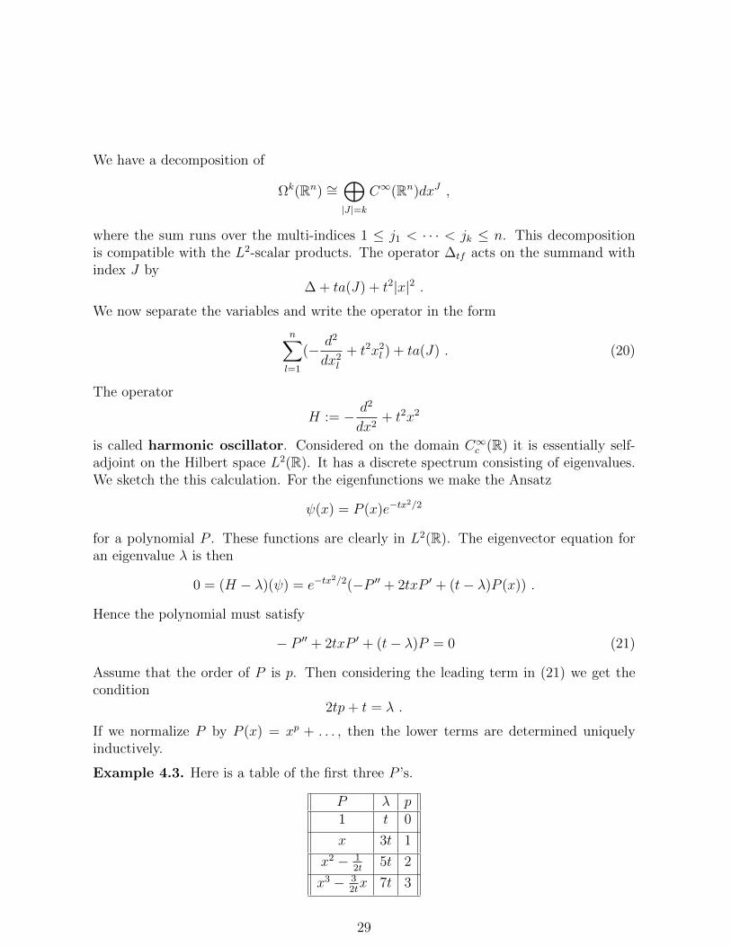
Example 4.3. Here is a table of the first three P ’s.

P λ p1 t 0

x 3t 1

x2 − 12t

5t 2

x3 − 32tx 7t 3

29

Thus we have found for every n ∈ N an eigenfunction of H of the form

ψ(x) := P (x)e−tx2/2 ,

where P (x) = xn +O(xn−1). The linear subspace

e−tx2/2P (x) | P ∈ C[x] ⊂ L2(R)

is dense. Hence we have found a complete set eigenfunctions. We can therefore concludethat the spectrum of H is the discrete set

2tp+ t | p ∈ N ⊂ R

and of multiplicity one.In view of (20) the eigenvalues of the Witten Laplacian

∆ + ta(J) + t2‖x‖2

acting as essentially selfadjoint operator on L2(Rn) with domain Ωc(Rn) are given by

2tp1 + · · ·+ 2tpn + tn+ ta(J) | (pi) ∈ Nn .

This set contains the value 0 if an only if J = (1, . . . , i). In this case it is represented bythe parameter (pi) = (0, . . . , 0) ∈ Nn and has with multiplicity one. The correspondingnormalized eigenvector is given by√

t

2π

n

e−t‖x‖2/2dx1 ∧ · · · ∧ dxi . (22)

If t→∞, then all non-zero eigenvalues tend linearly to ∞. Note that the second largesteigenvalue is 2t.

4.3 The spectrum of the Witten Laplacian

We now consider a closed manifold M with a self-indexing Morse function f . We canchoose the Riemannian metric gTM such that the Morse-Smale condition is satisfied,and such that the pair (f, gTM) near the critical points of f is is isomorphic to themodel case studied in Subsection 4.2. Let us call the domain of such an isomorphism astandard neighbourhood. Note that we can trivialize the bundle V in the standardneighbourhoods using the parallel transport associated to the flat connection.

We observe that for large t the eigenform (22) of the model operator concentrates at0. It can be transplanted to a standard neighbourhoods of the critical points. Aftermultiplication by a cut-off function which is constant near the critical point it can beextended to the whole manifold. Denote the result by φt. Then

‖φt‖L2 = 1 +O(e−ct) , ∆tfφt = O(e−ct)

30

exponentially. Moreover, these forms are mutually orthogonal for different critical points.We define a map

T it : Ci(V )→ Ωi(M)

which for x ∈ Critf (i) sends v ∈ Vx to the form T it (v) = φt ⊗ v. We further defineTt :=

∑Ti : C(V )→ Ω(M,V ).

We abbreviate H := L2(Ω(M,V )) and let

Ht[a, b] = Pt[a, b]H ⊆ H

be the spectral subspace of ∆tf for the interval [a, b] ⊆ R.

Theorem 4.4. 1. For every u, v ∈ C(V ) we have

〈Tt(u), Tt(v)〉 = 〈u, v〉+O(e−tc)

2. There exists positive constants C, c ∈ R such that for sufficiently large t ∈ R wehave

spec(∆tf ) ∩ [e−ct, Ct] = ∅ .

3. We have(1− Pt[0, 1])Tt = O(e−ct) ,

and

4.Pt[0, 1]Tt = Pt[0, 1] +O(e−ct) .

Proof. We have already explained the first and the third assertion. For the second weargue by contradiction. We assume that ψ is a normalized eigenvector of ∆tf for aneigenvalue λ ∈ [1, C]. We write

λ = 〈∆tfψ, ψ〉 = ‖dψ‖2 + ‖d∗ψ‖+ t〈A(f)ψ, ψ〉+ t2‖ |‖df‖ψ ‖2 . (23)

We conclude that most of the L2-norm of ψ must be concentrated near Critf . But here ∆tf

is equal to the model operator. One then decomposes ψ = ψ0 + ψ1, where ψ0 ∈ Im(Tt)and ψ1 ⊥ im(Tt). One can transplant ψ1 to the model case making an error of orderO(t−1). The resulting function is still orthogonal to the kernel of the model operator upto an error of the same order. Using the known spectrum of the model operator one getsan estimate

〈∆tfψ1, ψ1〉 ≥ Ct .

Furthermore〈∆tfψ0, ψ0〉 = O(e−ct) .

Finally, for the mixed terms we get

〈∆tfψ0, ψ1〉 = O(e−ct) .

31

These three inequalities together contradict (23). 2

Note that by Remark 4.1 we have an isomorphism ker(∆tf ) ∼= H(M,V). We get theMorse inequalities

Corollary 4.5. For all i ∈ N we have

dimH i(M,V) ≤ ]Critf (i) .

The idea to show the Morse inequalities in this way is die to Witten [Wit82].

4.4 The small eigenvalue complex

We now study the analytic torsion. We have a decomposition of the Hilbert space

H = Ht[0, 1]⊕Ht[C,∞] = Hsmallt ⊕H large

t

which is preserved by ∆tf . As remarked before we define the analytic torsion as inDefinition (2.8) but using ∆tf . We can decompose the analytic torsion correspondinglyas

Tan(M,∇V , hTM , hV ) = T smallan (t)T largean (t)

This induces a decomposition

TRS(M,∇V , hH(M,V)) := T smallRS (t) T largean (t) ,

whereT smallRS (t) := v(hH(M,V), h

H(M,V )Hodge (t)) T smallan (t) .

Theorem 4.6. We have limt→∞Tlargean (t) = 1.

The differential dtf preserves the small eigenvalue subspace Hsmallt . We can thus consider

the finite-dimensional complex (Hsmallt , dtf ). Its analytic torsion is T smallan (t). The main

point is now that this complex approximates (C(V ), d) for large t. This is much morecomplicated than the previous results. Here we use the restriction of the integration map

If : Hsmallt → C(V ) .

At this point we must understand the eigenvectors for large t not only near the criticalpoints, but also along the unstable manifolds W u(x). At this point one uses insights fromthe quantum mechanical study of tunnel effects. The details are to complicated to beexplained here. The original idea is due to Helffer-Sjstrand[HS85]. The final result is

Theorem 4.7.

limt→∞v(hH(M,V), hH(M,V )Hodge (t))T smallan (t) = Tan(C(V ), hV , hH(M,V)) .

32

References

[BFKM96] D. Burghelea, L. Friedlander, T. Kappeler, and P. McDonald. Analytic andReidemeister torsion for representations in finite type Hilbert modules. Geom.Funct. Anal., 6(5):751–859, 1996.

[BGV04] N. Berline, E. Getzler, and M. Vergne. Heat kernels and Dirac operators.Grundlehren Text Editions. Springer-Verlag, Berlin, 2004. Corrected reprint ofthe 1992 original.

[BZ92] Jean-Michel Bismut and Weiping Zhang. An extension of a theorem by Cheegerand Muller. Asterisque, (205):235, 1992. With an appendix by Francois Lauden-bach.

[Che79] Jeff Cheeger. Analytic torsion and the heat equation. Ann. of Math. (2),109(2):259–322, 1979.

[HS85] B. Helffer and J. Sjostrand. Puits multiples en mecanique semi-classique. IV.Etude du complexe de Witten. Comm. Partial Differential Equations, 10(3):245–340, 1985.

[M78] Werner Muller. Analytic torsion and R-torsion of Riemannian manifolds. Adv. inMath., 28(3):233–305, 1978.

[M93] Werner Muller. Analytic torsion and R-torsion for unimodular representations. J.Amer. Math. Soc., 6(3):721–753, 1993.

[RS71] D. B. Ray and I. M. Singer. R-torsion and the Laplacian on Riemannian manifolds.Advances in Math., 7:145–210, 1971.

[Wit82] Edward Witten. Supersymmetry and Morse theory. J. Differential Geom.,17(4):661–692 (1983), 1982.

33