Lectures on Astronomy, Astrophysics, and Cosmology

Luis A. AnchordoquiDepartment of Physics and Astronomy, Lehman College, City University of New York, NY 10468, USA

Department of Physics, Graduate Center, City University of New York, 365 Fifth Avenue, NY 10016, USADepartment of Astrophysics, American Museum of Natural History, Central Park West 79 St., NY 10024, USA

(Dated: Spring 2016)

This is a written version of a series of lectures aimed at undergraduate students in astrophysics/particletheory/particle experiment. We summarize the important progress made in recent years towardsunderstanding high energy astrophysical processes and we survey the state of the art regarding theconcordance model of cosmology.

I. ACROSS THE UNIVERSE

A look at the night sky provides a strong impression ofa changeless universe. We know that clouds drift acrossthe Moon, the sky rotates around the polar star, and onlonger times, the Moon itself grows and shrinks and theMoon and planets move against the background of stars.Of course we know that these are merely local phenom-ena caused by motions within our solar system. Farbeyond the planets, the stars appear motionless. Hereinwe are going to see that this impression of changeless-ness is illusory.

A. Nani gigantum humeris insidentes

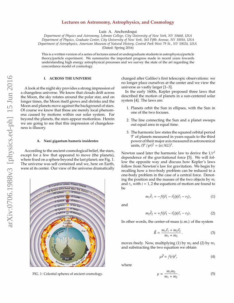
According to the ancient cosmological belief, the stars,except for a few that appeared to move (the planets),where fixed on a sphere beyond the last planet; see Fig. 1.The universe was self contained and we, here on Earth,were at its center. Our view of the universe dramatically

FIG. 1: Celestial spheres of ancient cosmology.

changed after Galileo’s first telescopic observations: weno longer place ourselves at the center and we view theuniverse as vastly larger [1–3].

In the early 1600s, Kepler proposed three laws thatdescribed the motion of planets in a sun-centered solarsystem [4]. The laws are:

1. Planets orbit the Sun in ellipses, with the Sun inone of the two focuses.

2. The line connecting the Sun and a planet sweepsout equal area in equal time.

3. The harmonic law states the squared orbital periodT of planets measured in years equals to the thirdpower of their major axis measured in astronomicalunits, (T /yr)2 = (a/AU)3.

Newton used later the harmonic law to derive the 1/r2

dependence of the gravitational force [5]. We will fol-low the opposite way and discuss how Kepler’s lawsfollow from Newton’s law for gravitation. We begin byrecalling how a two-body problem can be reduced to aone-body problem in the case of a central force. Denot-ing the position and the masses of the two objects by miand ri, with i = 1, 2 the equations of motion are found tobe

m1~r1 = − f (|~r1 − ~r2|)(~r1 − r2) , (1)

and

m2~r2 = + f (|~r1 − ~r2|)(~r1 − r2) . (2)

In other words, the center-of-mass (c.m.) of the system

~R =m1~r1 + m2~r2

m1 + m2. (3)

moves freely. Now, multiplying (1) by m2 and (2) by m1and substracting the two equation we obtain

µ~r = f (r)~r , (4)

where

µ =m1m2

m1 + m2. (5)

arX

iv:0

706.

1988

v3 [

phys

ics.

ed-p

h] 1

5 Ju

n 20

16

2

We can then solve a one-body problem for the reducedmass µ moving with the distance r = |~r1 − ~r2| in thegravitational field of the mass M = m1 + m2.

We can now derive the second law (a.k.a. the arealaw). Consider the movement of a body under the influ-ence of a central force (4). Since ~r × ~r = 0, the vectorialmultiplication of (4) by ~r leads to

µ~r × ~r = 0 , (6)

that looks already similar to a conservation law. Since

ddt

(~r × ~r) = ~r × ~r + ~r × ~r , (7)

the first term in the right-hand-side is zero and we obtainthe conservation of angular momentum ~L = µ~r × ~r forthe motion in a cental potential

µ~r × ~r =ddt

(µ~r × ~r) =ddt~L = 0 . (8)

There are two immediate consequences: First, the mo-tion is always in the plane perpendicular to ~L. Second,the area swept out by the vector ~r is

d ~A =12~r × ~v dt =

12µ

d~L , (9)

and thus also constant.We now turn to demonstrate the first law. We intro-

duce the unit vector r = ~r/r and rewrite the definition ofthe angular momentum ~L as

~L = µ~r × ~r = µrr ×ddt

(rr)

= µrr ×(rr + r

drdt

)= µr2r ×

drdt. (10)

The first term in the parenthesis vanishes, because of r×r = 0. Next we take the cross product of the gravitationalacceleration,

~a = −GMr2 r , (11)

with the angular momentum

~a ×~L = −GMr2 r ×

(µr2r ×

drdt

)= −GMµr ×

(r ×

drdt

), (12)

where G = 6.674×10−11 N m2 kg−2 [6]. The identity fromvector analysis, ~A× (~B× ~C) = ( ~A · ~C)~B− ( ~A · ~B)~C, leads to

~a ×~L = −GMµ

[(r ·

drdt

)r − (r · r)

drdt

]. (13)

Since r is a unit vector, we have r · r = 1 and d(r · r)/dt = 0,hence

~a ×~L = GMµdrdt. (14)

Since ~L and GMµ are constant, we can write this as

ddt

(~v ×~L) =ddt

(GMµr) . (15)

Integration of (15) leads to

~v ×~L = GMµr + ~C , (16)

where the integration constant ~C is a constant vector.Taking now the dot product with ~r, we have

~r · (~v ×~L) = GMµrr · r + ~r · ~C . (17)

Applying next the identity ~A · (~B × ~C) = ( ~A × ~B) · ~C, itfollows

(~r × ~v) ·~L = GMµr + rC cosϑ

= GMµr(1 +

C cosϑGMµ

), (18)

where ϑ is the angle between ~r and ~C. Expressing ~r × ~vas~L/µ, defining e = C/(GM) and solving for r, we obtainfinally the equation for a conic section, which is Kepler’sfirst law:

r =L2/µ2

GM(1 + e cosϑ). (19)

Using (A3) we obtain angular momentum

L = µ√

GMa(1 − e2) . (20)

To obtain the harmonic law we integrate the secondlaw in the form of (9) over one orbital period T ,

A = πab =L

2µT . (21)

Squaring and solving for T , it follows

T2 = 4π2 (abµ)2

L2 . (22)

Using (A1) and (20) for the angular momentum L, weobtain Kepler’s harmonic law,

T2 =

4π2

G(m1 + m2)a3 . (23)

EXERCISE 1.1 The planet Neptune, the most distantgas giant from the Sun, orbits with a semimajor axisa = 30.066 AU and an eccentricity e = 0.01. Pluto, the

3

next large world out from the Sun (though much smallerthan Neptune) orbits with a = 39.48 AU and e = 0.250.(i) To correct number of significant figures given theprecision of the data in this exercise, how many yearsdoes it take Neptune to orbit the Sun? (ii) How manyyears does it take Pluto to orbit the Sun? (iii) Take theratio of the two orbital periods you calculated in parts(i) and (ii). You will see that it is very close to the ratioof two small integers; which integers are these? Thusthe two planets regularly come close to one another,in the same part of their orbits, which allows them tohave a maximum gravitational influence on each other’sorbits. This is an example of an orbital resonance (otherexamples in the solar system can be found among themoons of Jupiter, and between the moons and variousfeatures of the rings of Saturn). (iv) What is the apheliondistance of Neptune’s orbit? Express your answer inAU. (v) What are the perihelion and aphelion distancesof Plutos orbit? Is Pluto always farther from the Sunthan Neptune?

EXERCISE 1.2 A satellite in geosynchronous orbit(GEO) orbits the Earth once every day. A satellite ingeostationary orbit (GSO) is a satellite in a circularGEO in the Earth’s equatorial plane. Therefore, fromthe point of view of an observer on Earth’s surface, asatellite in GSO seems always to hover in the same pointin the sky. For example, the satellites used for satelliteTV are in GSO so that satellite dishes can be stationaryand need not track their motion through the sky. Takea look; you will notice all satellite dishes on people’shouses point towards the Equator, that is South. Howfar above Earth’s equator (i.e., above the Earth’s surface)is a satellite in GSO? Express your answer in kilometers,and in Earth radii.

EXERCISE 1.3 The space station Mir traveled 3.6billion kilometers during its life. Its circular orbit was200 km above the surface of the Earth. (i) How manyyears was it in orbit? (ii) How many times did Mir circlethe Earth per day (i.e., 24 hours)? (iii) Can you put asatellite into such an orbit that it circles the Earth 20times per day?

The astronomical distances are so large that we specifythem in terms of the time it takes the light to travel a givendistance. For example, one light second = 3 × 108m =300, 000 km, one light minute = 1.8 × 107 km, and onelight year

1 ly = 9.46 × 1015 m ≈ 1013 km. (24)

For specifying distances to the Sun and the Moon, weusually use meters or kilometers, but we could spec-ify them in terms of light. The Earth-Moon distance is384,000 km, which is 1.28 ls. The Earth-Sun distance is150, 000, 000 km; this is equal to 8.3 lm. Far out in thesolar system, Pluto is about 6 × 109 km from the Sun, or6 × 10−4 ly. The nearest star to us, Proxima Centauri, is

about 4.2 ly away. Therefore, the nearest star is 10,000times farther from us that the outer reach of the solarsystem.

B. Stars and galaxies

On clear moonless nights, thousands of stars withvarying degrees of brightness can be seen, as well asthe long cloudy strip known as the Milky Way. Galileofirst observed with his telescope that the Milky Way iscomprised of countless numbers of individual stars. Ahalf century later Wright suggested that the Milky Waywas a flat disc of stars extending to great distances in aplane, which we call the Galaxy [7].

Our Galaxy has a diameter of 100,000 ly and a thick-ness of roughly 2,000 ly. It has a bulging central nucleusand spiral arms. Our Sun, which seems to be just an-other star, is located half way from the Galactic centerto the edge, some 26, 000 ly from the center. The Sunorbits the Galactic center approximately once every 250million years or so, so its speed is

v =2π 26, 000 × 1013 km

2.5 × 108 yr 3.156 × 107 s/yr= 200 km/s . (25)

The total mass of all the stars in the Galaxy can be esti-mated using the orbital data of the Sun about the centerof the Galaxy. To do so, assume that most of the massis concentrated near the center of the Galaxy and thatthe Sun and the solar system (of total mass m) move ina circular orbit around the center of the Galaxy (of totalmass M),

GMmr2 = m

v2

r, (26)

where a = v2/r is the centripetal acceleration. All in all,

M =r v2

G≈ 2 × 1041 kg . (27)

Assuming all the stars in the Galaxy are similar to ourSun (M ≈ 2 × 1030 kg), we conclude that there areroughly 1011 stars in the Galaxy.

In addition to stars both within and outside the MilkyWay, we can see with a telescope many faint cloudypatches in the sky which were once all referred to asnebulae (Latin for clouds). A few of these, such as those inthe constellations of Andromeda and Orion, can actuallybe discerned with the naked eye on a clear night. In theXVII and XVIII centuries, astronomers found that theseobjects were getting in the way of the search for comets.In 1781, in order to provide a convenient list of objects notto look at while hunting for comets, Messier publisheda celebrated catalogue [8]. Nowadays astronomers stillrefer to the 103 objects in this catalog by their Messiernumbers, e.g., the Andromeda Nebula is M31.

Even in Messier’s time it was clear that these extendedobjects are not all the same. Some are star clusters,

4

groups of stars which are so numerous that they ap-peared to be a cloud. Others are glowing clouds of gasor dust and it is for these that we now mainly reservethe word nebula. Most fascinating are those that belongto a third category: they often have fairly regular ellip-tical shapes and seem to be a great distance beyond theGalaxy. Kant seems to have been the first to suggest thatthese latter might be circular discs, but appear ellipticalbecause we see them at an angle, and are faint becausethey are so distant [9]. At first it was not universallyaccepted that these objects were extragalactic (i.e. out-side our Galaxy). The very large telescopes constructedin the XX century revealed that individual stars couldbe resolved within these extragalactic objects and thatmany contain spiral arms. Hubble did much of this ob-servational work in the 1920’s using the 2.5 m telescopeon Mt. Wilson near Los Angeles, California. Hubbledemostrated that these objects were indeed extragalac-tic because of their great distances [10]. The distance toour nearest spiral galaxy, Andromeda, is over 2 millionly, a distance 20 times greater than the diameter of ourGalaxy. It seemed logical that these nebulae must begalaxies similar to ours. Today it is thought that thereare roughly 4×1010 galaxies in the observable universe –that is, as many galaxies as there are stars in the Galaxy.

II. DISTANCE MEASUREMENTS

We have been talking about the vast distance of theobjects in the universe. We now turn to discuss differentmethods to estimate these distances.

A. Stellar Parallax

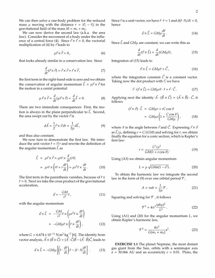
One basic method to measure distances to nearby starsemploys simple geometry and stellar parallax. Parallaxis the apparent displacement of an object because of achange in the observer’s point of view. One way to seehow this effect works is to hold your hand out in frontof you and look at it with your left eye closed, thenyour right eye closed. Your hand will appear to moveagainst the background. By stellar parallax we meanthe apparent motion of a star against the backgroundof more distant stars, due to Earth’s motion around theSun; see Fig. 2. The sighting angle of a star relativeto the plane of Earth’s orbit (usually indicated by θ)can be determined at two different times of the yearseparated by six months. Since we know the distance dfrom the Earth to the Sun, we can determine the distanceD to the star. For example, if the angle θ of a givenstar is measured to be 89.99994, the parallax angle isp ≡ φ = 0.00006. From trigonometry, tanφ = d/D, andsince the distance to the Sun is d = 1.5 × 108 km thedistance to the star is

D =d

tanφ≈

dφ

=1.5 × 108 km

1 × 10−6 = 1.5 × 1014 km , (28)

FIG. 2: The parallax method of measuring a star’s distance.

or about 15 ly.Distances to stars are often specified in terms of paral-

lax angles given in seconds of arc: 1 second (1”) is 1/60of a minute (1’) of arc, which is 1/60 of a degree, so 1”= 1/3600 of a degree. The distance is then specified inparsecs (meaning parallax angle in seconds of arc), wherethe parsec is defined as 1/φ with φ in seconds. For ex-ample, if φ = 6 × 10−5 , we would say the the star is at adistance D = 4.5 pc.

The angular resolution of the Hubble Space Telescope(HST) is about 1/20 arcs. With HST one can measureparallaxes of about 2 milli arc seconds (e.g., 1223Sgr). This corresponds to a distance of about 500 pc.Besides, there are stars with radio emission for whichobservations from the Very Long Baseline Array (VLBA)allow accurate parallax measurements beyond 500 pc.For example, parallax measurements of Sco X-1 are0.36±0.04 milli arc seconds which puts it at a distance of2.8 kpc. Parallax can be used to determine the distanceto stars as far away as about 3 kpc from Earth. Beyondthat distance, parallax angles are two small to measureand more subtle techniques must be employed.

EXERCISE 2.1 One of the first people to make a veryaccurate measurement of the circumference of the Earthwas Eratosthenes, a Greek philosopher who lived inAlexandria around 250 B.C. He was told that on a cer-tain day during the summer (June 21) in a town calledSyene, which was 4900 stadia (1 stadia = 0.16 kilometers)to the south of Alexandria, the sunlight shown directlydown the well shafts so that you could see all the way tothe bottom. Eratosthenes knew that the sun was neverquite high enough in the sky to see the bottom of wellsin Alexandria and he was able to calculate that in factit was about 7 degrees too low. Knowing that the sunwas 7 degrees lower at its highpoint in Alexandria thanin Syene and assuming that the sun’s rays were paral-lel when they hit the Earth, Eratosthenes was able to

51 Continuous radiation from stars

ϑ

dΩ

dA

cos ϑdA

ϑ

dΩ

dA

cos ϑdA

Figure 1.3: Left: A detector with surface element dA on Earth measuring radiation comingfrom a direction with zenith angle ϑ. Right: An imaginary detector on the surfaceof a star measuring radiation emitted in the direction ϑ.

The Kirchhoff-Planck distribution contains as its two limiting cases Wien’s law for high-frequencies, hν ≫ kT , and the Rayleigh-Jeans law for low-frequencies hν ≪ kT . In theformer limit, x = hν/(kT ) ≫ 1, and we can neglect the −1 in the denominator of the Planckfunction,

Bν ≈ 2hν3

c2exp(−hν/kT ) . (1.10)

Thus the number of photons with energy hν much larger than kT is exponentially suppressed.In the opposite limit, x = hν/(kT ) ≪ 1, and ex − 1 = (1 + x − . . .) − 1 ≈ x. Hence Planck’sconstant h disappears from the expression for Bν , if the energy hν of a single photon is smallcompared to the thermal energy kT and one obtains,

Bν ≈ 2ν2kT

c2. (1.11)

The Rayleigh-Jeans law shows up as straight lines left from the maxima of Bν in Fig. 1.4.

1.3.2 Wien’s displacement law

We note from Fig. 1.4 two important properties of Bν : Firstly, Bν as function of the frequencyν has a single maximum. Secondly, Bν as function of the temperature T is a monotonicallyincreasing function for all frequencies: If T1 > T2, then Bν(T1) > Bν(T2) for all ν. Bothproperties follow directly from taking the derivative with respect to ν and T . In the formercase, we look for the maximum of f(ν) = c2

2hBν as function of ν. Hence we have to find thezeros of f ′(ν),

3(ex − 1) − x expx = 0 with x =hν

kT. (1.12)

The equation ex(3 − x) = 3 has to be solved numerically and has the solution x ≈ 2.821.Thus the intensity of thermal radiation is maximal for xmax ≈ 2.821 = hνmax/(kT ) or

cT

νmax≈ 0.50K cm or

νmax

T≈ 5.9 × 1010Hz/K . (1.13)

14

cos dA

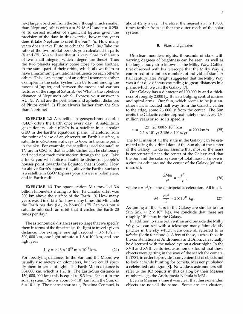
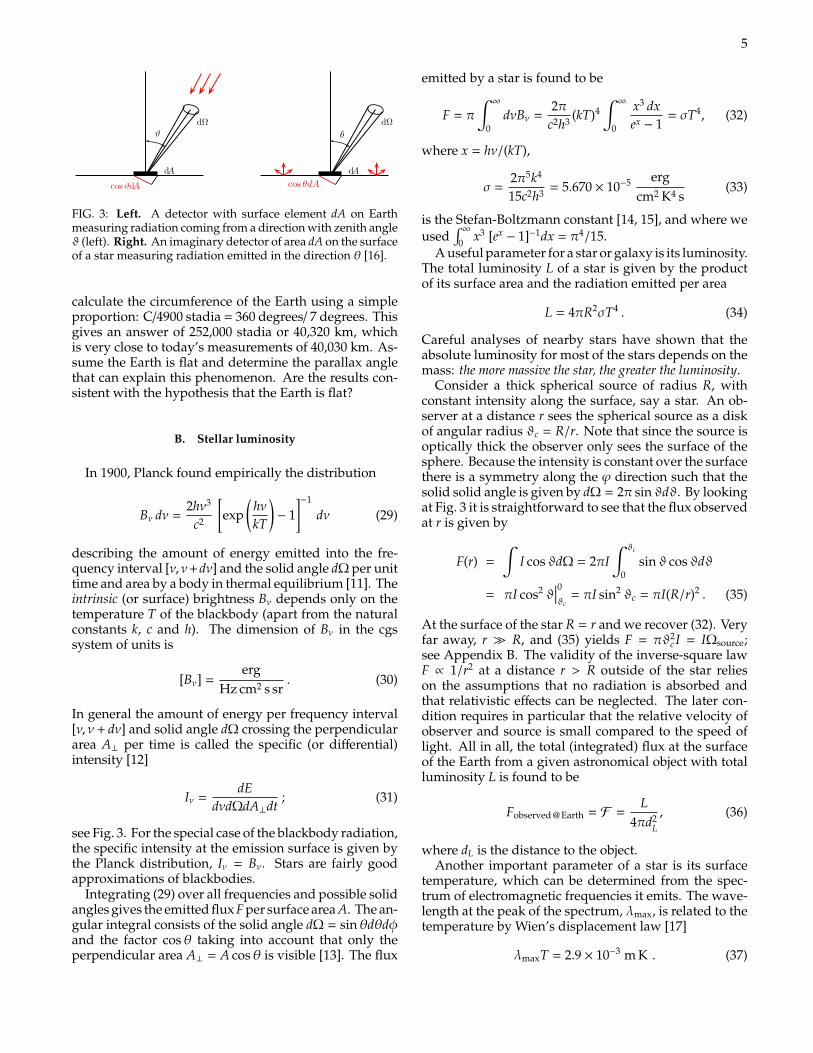
FIG. 3: Left. A detector with surface element dA on Earthmeasuring radiation coming from a direction with zenith angleϑ (left). Right. An imaginary detector of area dA on the surfaceof a star measuring radiation emitted in the direction θ [16].

calculate the circumference of the Earth using a simpleproportion: C/4900 stadia = 360 degrees/ 7 degrees. Thisgives an answer of 252,000 stadia or 40,320 km, whichis very close to today’s measurements of 40,030 km. As-sume the Earth is flat and determine the parallax anglethat can explain this phenomenon. Are the results con-sistent with the hypothesis that the Earth is flat?

B. Stellar luminosity

In 1900, Planck found empirically the distribution

Bν dν =2hν3

c2

[exp

(hνkT

)− 1

]−1

dν (29)

describing the amount of energy emitted into the fre-quency interval [ν, ν+dν] and the solid angle dΩ per unittime and area by a body in thermal equilibrium [11]. Theintrinsic (or surface) brightness Bν depends only on thetemperature T of the blackbody (apart from the naturalconstants k, c and h). The dimension of Bν in the cgssystem of units is

[Bν] =erg

Hz cm2 s sr. (30)

In general the amount of energy per frequency interval[ν, ν+ dν] and solid angle dΩ crossing the perpendiculararea A⊥ per time is called the specific (or differential)intensity [12]

Iν =dE

dνdΩdA⊥dt; (31)

see Fig. 3. For the special case of the blackbody radiation,the specific intensity at the emission surface is given bythe Planck distribution, Iν = Bν. Stars are fairly goodapproximations of blackbodies.

Integrating (29) over all frequencies and possible solidangles gives the emitted flux F per surface area A. The an-gular integral consists of the solid angle dΩ = sinθdθdφand the factor cosθ taking into account that only theperpendicular area A⊥ = A cosθ is visible [13]. The flux

emitted by a star is found to be

F = π

∫∞

0dνBν =

2πc2h3 (kT)4

∫∞

0

x3 dxex − 1

= σT4, (32)

where x = hν/(kT),

σ =2π5k4

15c2h3 = 5.670 × 10−5 ergcm2 K4 s

(33)

is the Stefan-Boltzmann constant [14, 15], and where weused

∫∞

0 x3 [ex− 1]−1dx = π4/15.

A useful parameter for a star or galaxy is its luminosity.The total luminosity L of a star is given by the productof its surface area and the radiation emitted per area

L = 4πR2σT4 . (34)

Careful analyses of nearby stars have shown that theabsolute luminosity for most of the stars depends on themass: the more massive the star, the greater the luminosity.

Consider a thick spherical source of radius R, withconstant intensity along the surface, say a star. An ob-server at a distance r sees the spherical source as a diskof angular radius ϑc = R/r. Note that since the source isoptically thick the observer only sees the surface of thesphere. Because the intensity is constant over the surfacethere is a symmetry along the ϕ direction such that thesolid solid angle is given by dΩ = 2π sinϑdϑ. By lookingat Fig. 3 it is straightforward to see that the flux observedat r is given by

F(r) =

∫I cosϑdΩ = 2πI

∫ ϑc

0sinϑ cosϑdϑ

= πI cos2 ϑ∣∣∣0ϑc

= πI sin2 ϑc = πI(R/r)2 . (35)

At the surface of the star R = r and we recover (32). Veryfar away, r R, and (35) yields F = πϑ2

c I = IΩsource;see Appendix B. The validity of the inverse-square lawF ∝ 1/r2 at a distance r > R outside of the star relieson the assumptions that no radiation is absorbed andthat relativistic effects can be neglected. The later con-dition requires in particular that the relative velocity ofobserver and source is small compared to the speed oflight. All in all, the total (integrated) flux at the surfaceof the Earth from a given astronomical object with totalluminosity L is found to be

Fobserved @ Earth = F =L

4πd2L

, (36)

where dL is the distance to the object.Another important parameter of a star is its surface

temperature, which can be determined from the spec-trum of electromagnetic frequencies it emits. The wave-length at the peak of the spectrum, λmax, is related to thetemperature by Wien’s displacement law [17]

λmaxT = 2.9 × 10−3 m K . (37)

6

We can now use Wien’s law and the Steffan-Boltzmannequation (power output or luminosity ∝ AT4) to deter-mine the temperature and the relative size of a star. Sup-pose that the distance from Earth to two nearby starscan be reasonably estimated, and that their apparent lu-minosities suggest the two stars have about the sameabsolute luminosity, L. The spectrum of one of the starspeaks at about 700 nm (so it is reddish). The spectrum ofthe other peaks at about 350 nm (bluish). Using Wien’slaw, the temperature of the reddish star is Tr ' 4140 K.The temperature of the bluish star will be double becauseits peak wavelength is half, Tb ' 8280 K. The power ra-diated per unit of area from a star is proportional to thefourth power of the Kelvin temperature (34). Now thetemperature of the bluish star is double that of the redishstar, so the bluish must radiate 16 times as much energyper unit area. But we are given that they have the sameluminosity, so the surface area of the blue star must be1/16 that of the red one. Since the surface area is 4πR2,we conclude that the radius of the redish star is 4 timeslarger than the radius of the bluish star (and its volume64 times larger) [18].

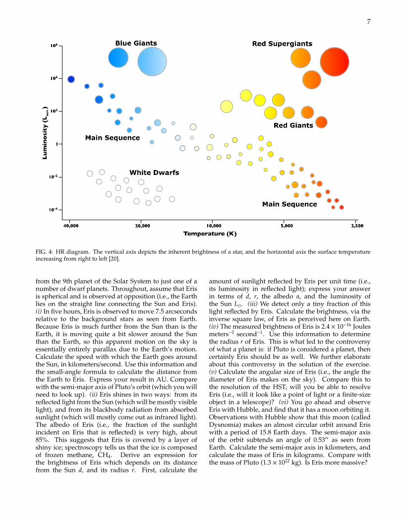
An important astronomical discovery, made around1900, was that for most of the stars, the color is relatedto the absolute luminosity and therefore to the mass.A useful way to present this relationship is by the so-called Hertzsprung-Russell (HR) diagram [19]. On theHR diagram, the horizontal axis shows the temperatureT, whereas the vertical axis the luminosity L, each star isrepresented by a point on the diagram shown in Fig. 4.Most of the stars fall along the diagonal band termed themain sequence. Starting at the lowest right, we find thecoolest stars, redish in color; they are the least luminousand therefore low in mass. Further up towards the leftwe find hotter and more luminous stars that are whitishlike our Sun. Still farther up we find more massive andmore luminous stars, bluish in color. There are also starsthat fall outside the main sequence. Above and to theright we find extremely large stars, with high luminositybut with low (redish) color temperature: these are calledred giants. At the lower left, there are a few stars of lowluminosity but with high temperature: these are whitedwarfs.

Suppose that a detailed study of a certain star suggeststhat it most likely fits on the main sequence of the HRdiagram. The observed flux is F = 1× 10−12 W m−2, andthe peak wavelength of its spectrum is λmax ≈ 600 nm.We can first find the temperature using Wien’s lawand then estimate the absolute luminosity using theHR diagram; namely, T ≈ 4800 K. A star on the mainsequence of the HR diagram at this temperature hasabsolute luminosity of about L ≈ 1026 W. Then, using(36) we can estimate its distance from us, dL = 3× 1018 mor equivalently 300 ly.

EXERCISE 2.2 About 1350 J of energy strikes theatmosphere of the Earth from the Sun per secondper square meter of area at right angle to the Sun’s

rays. What is (i) the observed flux from the Sun Fand (ii) its absolute luminosity L. (iii) What is theaverage Solar flux density measured at Mars? (iv) If theapproximate efficiency of the solar panels (with area of1.3 m2) on the Martian rover Spirit is 20%, then howmany Watts could the fully illuminated panels generate?

EXERCISE 2.3 Suppose the MESSENGER spacecraft,while orbiting Mercury, decided to communicate withthe Cassini probe, now exploring Saturn and its moons.When Mercury is closest to Saturn in their orbits, ittakes 76.3 minutes for the radio signals from Mercuryto reach Saturn. A little more than half a mercurianyear later, when the 2 planets are furthest apart in theirorbits, it takes 82.7 minutes. (i) What is the distancebetween Mercury and the Sun? Give answers in bothlight-minutes and astronomical units. Assume that theplanets have circular orbits. (ii) What is the distancebetween Saturn and the Sun?

EXERCISE 2.4 The photometric method to search forextrasolar planets is based on the detection of stellarbrightness variations, which result from the transit of aplanet across a star’s disk. If a planet passes in front ofa star, the star will be partially eclipsed and its light willbe dimmed. Determine the reduction in the apparentsurface brightness I when Jupiter passes in front of theSun.

EXERCISE 2.5 The angular resolution of a telescope(or other optical system) is a measure of the smallestdetails which can be seen. Because of the distortingeffects of earth’s atmosphere, the best angular resolutionwhich can be achieved by optical telescopes from earth’ssurface is normally about 1 arcs. This is why muchclearer images can be obtained from space. The angularresolution of the HST is about 0.05 arcs, and the smallestangle that can be measured accurately with HST isactually a fraction of one resolution element. (i) Cepheidvariable stars are very important distance indicatorsbecause they have large and well-known luminosities.What is the distance of a Cepheid variable star whoseparallax angle is measured to be 0.005 ± 0.001 arcs?(ii) The faintest stars that can be detected with the HSThave apparent brightnesses which are 4 × 1021 timesfainter than the Sun. How far away could a star likethe Sun be, and still be detected with the HST? Expressyour answer in light years. (iii) How far away could aCepheid variable with 20,000 times the luminosity ofthe Sun be, and still be detected with the HST? Expressyour answer in light years.

EXERCISE 2.6 The discovery of the dwarf planetEris in 2005 threw the astronomical community into atizzy and made international headlines; it is slightlylarger than Pluto and brought up interesting questionsabout what the definition of a planet is. Eventually,this resulted in the controversial demotion of Pluto

7

AST 250 Spring 2010 HOMEWORK #5

Due Friday March 26

(1) Develop you own mnemonic for the modern stellar spectral sequence:

O B A F G K M L T Y. Be creative! I’ll read a few in class.

(2) Look up the spectral types of the following stars (the primary stars if it is a binary) and order them by (a) effective temperature and (b) luminosity: Sun, Sirius, Betlegeuse, Aldebaran, and Barnard’s Star. (N.B. don’t just look up Teff and L. Understand the ordering based on spectral type. There could be a similar question on the exam).

(3) Estimate the mass of main sequence stars with twice the luminosity of the Sun and with half the luminosity of the Sun. What is the dominant nucleosynthesis process in the cores of these stars?

(4) Calculate the Schwarzchild radius for a star the mass of the Sun.

(5) (a) The Hertzsprung-Russell diagram is usually plotted in logarithmic

coordinates (log L vs. log Teff with temperature increasing to the left). Mathematically derive the slope of a line of constant radius in the logarithmic H-R diagram. (b) Order the stars in problem 2 by stellar radii.

FIG. 4: HR diagram. The vertical axis depicts the inherent brightness of a star, and the horizontal axis the surface temperatureincreasing from right to left [20].

from the 9th planet of the Solar System to just one of anumber of dwarf planets. Throughout, assume that Erisis spherical and is observed at opposition (i.e., the Earthlies on the straight line connecting the Sun and Eris).(i) In five hours, Eris is observed to move 7.5 arcsecondsrelative to the background stars as seen from Earth.Because Eris is much further from the Sun than is theEarth, it is moving quite a bit slower around the Sunthan the Earth, so this apparent motion on the sky isessentially entirely parallax due to the Earth’s motion.Calculate the speed with which the Earth goes aroundthe Sun, in kilometers/second. Use this information andthe small-angle formula to calculate the distance fromthe Earth to Eris. Express your result in AU. Comparewith the semi-major axis of Pluto’s orbit (which you willneed to look up). (ii) Eris shines in two ways: from itsreflected light from the Sun (which will be mostly visiblelight), and from its blackbody radiation from absorbedsunlight (which will mostly come out as infrared light).The albedo of Eris (i.e., the fraction of the sunlightincident on Eris that is reflected) is very high, about85%. This suggests that Eris is covered by a layer ofshiny ice; spectroscopy tells us that the ice is composedof frozen methane, CH4. Derive an expression forthe brightness of Eris which depends on its distancefrom the Sun d, and its radius r. First, calculate the

amount of sunlight reflected by Eris per unit time (i.e.,its luminosity in reflected light); express your answerin terms of d, r, the albedo a, and the luminosity ofthe Sun L. (iii) We detect only a tiny fraction of thislight reflected by Eris. Calculate the brightness, via theinverse square law, of Eris as perceived here on Earth.(iv) The measured brightness of Eris is 2.4 × 10−16 Joulesmeters−2 second−1. Use this information to determinethe radius r of Eris. This is what led to the controversyof what a planet is: if Pluto is considered a planet, thencertainly Eris should be as well. We further elaborateabout this controversy in the solution of the exercise.(v) Calculate the angular size of Eris (i.e., the angle thediameter of Eris makes on the sky). Compare this tothe resolution of the HST; will you be able to resolveEris (i.e., will it look like a point of light or a finite-sizeobject in a telescope)? (vi) You go ahead and observeEris with Hubble, and find that it has a moon orbiting it.Observations with Hubble show that this moon (calledDysnomia) makes an almost circular orbit around Eriswith a period of 15.8 Earth days. The semi-major axisof the orbit subtends an angle of 0.53′′ as seen fromEarth. Calculate the semi-major axis in kilometers, andcalculate the mass of Eris in kilograms. Compare withthe mass of Pluto (1.3 × 1022 kg). Is Eris more massive?

8

EXERCISE 2.7 A perfect blackbody at temperature Thas the shape of an oblate ellipsoid, its surface beinggiven by the equation

x2

a2 +y2

a2 +z2

b2 = 1 , (38)

with a > b. (i) Is the luminosity of the blackbodyisotropic? Why? (ii) Consider an observer at a distancedL from the blackbody, with dL a. What is the direc-tion of the observer for which the maximum amount offlux will be observed (keeping the distance dL fixed)?Calculate what this maximum flux is. (iii) Repeat thesame exercise for the direction for which the minimumflux will be observed, for fixed dL. (iv) If the twoobservers who see the maximum and minimum fluxfrom distance dL can resolve the blackbody, what isthe apparent brightness, I, that each one will measure?(v) Write down an expression for the total luminosityemitted by the black body as a function of a, b andT. (vi) Now, consider a galaxy with a perfectly oblateshape, which contains only a large number N of stars,and no gas or dust. To make it simple, assume that allstars have radius R and surface temperature T. Answeragain the questions (i-v) for the galaxy, assumingNR2

ab. Are there any differences from the case of ablackbody? Explain why. (vii) Imagine that there werea very compact galaxy that did not obey the conditionNR2

ab. Would the answer to the previous questionbe modified? Do you think such a galaxy could be stable?

EXERCISE 2.8 The HR diagram is usually plotted inlogarithmic coordinates (log L vs. log T, with the tem-perature increasing to the left). Derive the slope of a lineof constant radius in the logarithmic HR diagram.

III. DOPPLER EFFECT

There is observational evidence that stars move atspeeds ranging up to a few hundred kilometers persecond, so in a year a fast moving star might travel∼ 1010 km. This is 103 times less than the distance to theclosest star, so their apparent position in the sky changesvery slowly. For example, the relatively fast movingstar known as Barnard’s star is at a distance of about56 × 1012 km; it moves across the line of sight at about89 km/s, and in consequence its apparent position shifts(so-called “proper motion”) in one year by an angle of0.0029 degrees. The HST has measured proper motionsas low as about 1 milli arc second per year. In the radio(VLBA), relative motions can be measured to an accu-racy of about 0.2 milli arc second per year. The apparentposition in the sky of the more distant stars changes soslowly that their proper motion cannot be detected witheven the most patient observation. However, the rateof approach or recession of a luminous body in the lineof sight can be measured much more accurately than itsmotion at right angles to the line of sight. The technique

makes use of a familiar property of any sort of wavemotion, known as Doppler effect [21].

When we observe a sound or light wave from a sourceat rest, the time between the arrival wave crests at ourinstruments is the same as the time between crests as theyleave the source. However, if the source is moving awayfrom us, the time between arrivals of successive wavecrests is increased over the time between their departuresfrom the source, because each crest has a little farther togo on its journey to us than the crest before. The timebetween crests is just the wavelength divided by thespeed of the wave, so a wave sent out by a source movingaway from us will appear to have a longer wavelengththan if the source were at rest. Likewise, if the source ismoving toward us, the time between arrivals of the wavecrests is decreased because each successive crest has ashorter distance to go, and the waves appear to have ashorter wavelength. A nice analogy was put forwardby Weinberg [22]. He compared the situation with atravelling man that has to send a letter home regularlyonce a week during his travels: while he is travellingaway from home, each successive letter will have a littlefarther to go than the one before, so his letters will arrivea little more than a week apart; on the homeward legof his journey, each succesive letter will have a shorterdistance to travel, so they will arrive more frequentlythan once a week.

The Doppler effect began to be of enormous impor-tance to astronomy in 1968, when it was applied to thestudy of individual spectral lines. In 1815, Fraunhoferfirst realized that when light from the Sun is allowed topass through a slit and then through a glass prism, theresulting spectrum of colors is crossed with hundreds ofdark lines, each one an image of the slit [23]. The darklines were always found at the same colors, each corre-sponding to a definite wavelength of light. The samedark spectral lines were also found in the same posi-tion in the spectrum of the Moon and brighter stars. Itwas soon realized that these dark lines are produced bythe selective absorption of light of certain definite wave-lengths, as light passes from the hot surface of a starthrough its cooler outer atmosphere. Each line is due toabsorption of light by a specific chemical element, so itbecame possible to determine that the elements on theSun, such as sodium, iron, magnesium, calcium, andchromium, are the same as those found on Earth.

In 1868, Sir Huggins was able to show that the darklines in the spectra of some of the brighter stars areshifted slightly to the red or the blue from their normalposition in the spectrum of the Sun [24]. He correctlyinterpreted this as a Doppler shift, due to the motion ofthe star away from or toward the Earth. For example, thewavelength of every dark line in the spectrum of the starCapella is longer than the wavelength of the correspond-ing dark line in the spectrum of the Sun by 0.01%, thisshift to the red indicates that Capella is receding fromus at 0.01% c (i.e., the radial velocity of Capella is about30 km/s).

9

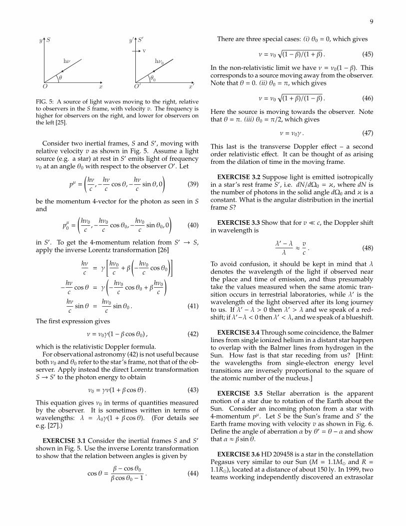
FIG. 5: A source of light waves moving to the right, relativeto observers in the S frame, with velocity v. The frequency ishigher for observers on the right, and lower for observers onthe left [25].

Consider two inertial frames, S and S′, moving withrelative velocity v as shown in Fig. 5. Assume a lightsource (e.g. a star) at rest in S′ emits light of frequencyν0 at an angle θ0 with respect to the observer O′. Let

pµ =

(hνc,−

hνc

cosθ,−hνc

sinθ, 0)

(39)

be the momentum 4-vector for the photon as seen in Sand

pµ0 =

(hν0

c,−

hν0

ccosθ0,−

hν0

csinθ0, 0

)(40)

in S′. To get the 4-momentum relation from S′ → S,apply the inverse Lorentz transformation [26]

hνc

= γ

[hν0

c+ β

(−

hν0

ccosθ0

)]−

hνc

cosθ = γ

(−

hν0

ccosθ0 + β

hν0

c

)hνc

sinθ =hν0

csinθ0 . (41)

The first expression gives

ν = ν0γ(1 − β cosθ0) , (42)

which is the relativistic Doppler formula.For observational astronomy (42) is not useful because

both ν0 and θ0 refer to the star’s frame, not that of the ob-server. Apply instead the direct Lorentz transformationS→ S′ to the photon energy to obtain

ν0 = γν(1 + β cosθ) . (43)

This equation gives ν0 in terms of quantities measuredby the observer. It is sometimes written in terms ofwavelengths: λ = λ0γ(1 + β cosθ). (For details seee.g. [27].)

EXERCISE 3.1 Consider the inertial frames S and S′shown in Fig. 5. Use the inverse Lorentz transformationto show that the relation between angles is given by

cosθ =β − cosθ0

β cosθ0 − 1. (44)

There are three special cases: (i) θ0 = 0, which gives

ν = ν0√

(1 − β)/(1 + β) . (45)

In the non-relativistic limit we have ν = ν0(1 − β). Thiscorresponds to a source moving away from the observer.Note that θ = 0. (ii) θ0 = π, which gives

ν = ν0√

(1 + β)/(1 − β) . (46)

Here the source is moving towards the observer. Notethat θ = π. (iii) θ0 = π/2, which gives

ν = ν0γ . (47)

This last is the transverse Doppler effect – a secondorder relativistic effect. It can be thought of as arisingfrom the dilation of time in the moving frame.

EXERCISE 3.2 Suppose light is emitted isotropicallyin a star’s rest frame S′, i.e. dN/dΩ0 = κ, where dN isthe number of photons in the solid angle dΩ0 and κ is aconstant. What is the angular distribution in the inertialframe S?

EXERCISE 3.3 Show that for v c, the Doppler shiftin wavelength is

λ′ − λλ

≈vc. (48)

To avoid confusion, it should be kept in mind that λdenotes the wavelength of the light if observed nearthe place and time of emission, and thus presumablytake the values measured when the same atomic tran-sition occurs in terrestrial laboratories, while λ′ is thewavelength of the light observed after its long journeyto us. If λ′ − λ > 0 then λ′ > λ and we speak of a red-shift; ifλ′−λ < 0 thenλ′ < λ, and we speak of a blueshift.

EXERCISE 3.4 Through some coincidence, the Balmerlines from single ionized helium in a distant star happento overlap with the Balmer lines from hydrogen in theSun. How fast is that star receding from us? [Hint:the wavelengths from single-electron energy leveltransitions are inversely proportional to the square ofthe atomic number of the nucleus.]

EXERCISE 3.5 Stellar aberration is the apparentmotion of a star due to rotation of the Earth about theSun. Consider an incoming photon from a star with4-momentum pµ. Let S be the Sun’s frame and S′ theEarth frame moving with velocity v as shown in Fig. 6.Define the angle of aberration α by θ′ = θ − α and showthat α ≈ β sinθ.

EXERCISE 3.6 HD 209458 is a star in the constellationPegasus very similar to our Sun (M = 1.1M and R =1.1R), located at a distance of about 150 ly. In 1999, twoteams working independently discovered an extrasolar

10

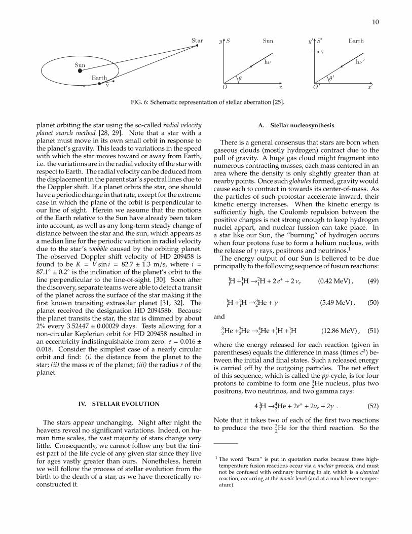
FIG. 6: Schematic representation of stellar aberration [25].

planet orbiting the star using the so-called radial velocityplanet search method [28, 29]. Note that a star with aplanet must move in its own small orbit in response tothe planet’s gravity. This leads to variations in the speedwith which the star moves toward or away from Earth,i.e. the variations are in the radial velocity of the star withrespect to Earth. The radial velocity can be deduced fromthe displacement in the parent star’s spectral lines due tothe Doppler shift. If a planet orbits the star, one shouldhave a periodic change in that rate, except for the extremecase in which the plane of the orbit is perpendicular toour line of sight. Herein we assume that the motionsof the Earth relative to the Sun have already been takeninto account, as well as any long-term steady change ofdistance between the star and the sun, which appears asa median line for the periodic variation in radial velocitydue to the star’s wobble caused by the orbiting planet.The observed Doppler shift velocity of HD 209458 isfound to be K = V sin i = 82.7 ± 1.3 m/s, where i =87.1 ± 0.2 is the inclination of the planet’s orbit to theline perpendicular to the line-of-sight. [30]. Soon afterthe discovery, separate teams were able to detect a transitof the planet across the surface of the star making it thefirst known transiting extrasolar planet [31, 32]. Theplanet received the designation HD 209458b. Becausethe planet transits the star, the star is dimmed by about2% every 3.52447 ± 0.00029 days. Tests allowing for anon-circular Keplerian orbit for HD 209458 resulted inan eccentricity indistinguishable from zero: e = 0.016 ±0.018. Consider the simplest case of a nearly circularorbit and find: (i) the distance from the planet to thestar; (ii) the mass m of the planet; (iii) the radius r of theplanet.

IV. STELLAR EVOLUTION

The stars appear unchanging. Night after night theheavens reveal no significant variations. Indeed, on hu-man time scales, the vast majority of stars change verylittle. Consequently, we cannot follow any but the tini-est part of the life cycle of any given star since they livefor ages vastly greater than ours. Nonetheless, hereinwe will follow the process of stellar evolution from thebirth to the death of a star, as we have theoretically re-constructed it.

A. Stellar nucleosynthesis

There is a general consensus that stars are born whengaseous clouds (mostly hydrogen) contract due to thepull of gravity. A huge gas cloud might fragment intonumerous contracting masses, each mass centered in anarea where the density is only slightly greater than atnearby points. Once such globules formed, gravity wouldcause each to contract in towards its center-of-mass. Asthe particles of such protostar accelerate inward, theirkinetic energy increases. When the kinetic energy issufficiently high, the Coulomb repulsion between thepositive charges is not strong enough to keep hydrogennuclei appart, and nuclear fussion can take place. Ina star like our Sun, the “burning” of hydrogen occurswhen four protons fuse to form a helium nucleus, withthe release of γ rays, positrons and neutrinos.1

The energy output of our Sun is believed to be dueprincipally to the following sequence of fusion reactions:

11H +1

1H→21H + 2 e+ + 2 νe (0.42 MeV) , (49)

11H +2

1H→32He + γ (5.49 MeV) , (50)

and

32He +3

2He→42He +1

1H +11H (12.86 MeV) , (51)

where the energy released for each reaction (given inparentheses) equals the difference in mass (times c2) be-tween the initial and final states. Such a released energyis carried off by the outgoing particles. The net effectof this sequence, which is called the pp-cycle, is for fourprotons to combine to form one 4

2He nucleus, plus twopositrons, two neutrinos, and two gamma rays:

4 11H→

42He + 2e+ + 2νe + 2γ . (52)

Note that it takes two of each of the first two reactionsto produce the two 3

2He for the third reaction. So the

1 The word “burn” is put in quotation marks because these high-temperature fusion reactions occur via a nuclear process, and mustnot be confused with ordinary burning in air, which is a chemicalreaction, occurring at the atomic level (and at a much lower temper-ature).

11

total energy released for the net reaction is 24.7 MeV.However, each of the two e+ quickly annihilates withan electron to produce 2mec2 = 1.02 MeV; so the totalenergy released is 26.7 MeV. The first reaction, theformation of deuterium from two protons, has very lowprobability, and the infrequency of that reaction servesto limit the rate at which the Sun produces energy.These reactions requiere a temperature of about 107 K,corresponding to an average kinetic energy (kT) of 1 keV.

EXERCISE 4.1 Approximately 1038 neutrinos areproduced by the pp chain in the Sun every second.Calculate the number of neutrinos from the Sun that arepassing through your brain every second.

In more massive stars, it is more likely that the energyoutput comes principally from the carbon (or CNO) cy-cle, which comprises the following sequence of reactions:

126C +1

1H→137N + γ , (53)

137N→

136C + e+ + ν , (54)

136C +1

1H→147N + γ , (55)

147N +1

1H→158O + γ , (56)

158O→

157N + e+ + ν , (57)

157N +1

1H→126C +4

2He . (58)

It is easily seen that no carbon is consumed in this cycle(see first and last equations) and that the net effect is thesame as the pp cycle. The theory of the pp cycle and thecarbon cycle as the source of energy for the Sun and thestars was first worked out by Bethe in 1939 [33].

The fusion reactions take place primarily in the coreof the star, where T is sufficiently high. (The surfacetemperature is of course much lower, on the order ofa few thousand K.) The tremendous release of energyin these fusion reactions produces an outward pressuresufficient to halt the inward gravitational contraction;and our protostar, now really a young star, stabilizes inthe main sequence.

To a good approximation the stellar structure on themain sequence can be described by a spherically sym-metric system in hydrostatic equilibrium. This requiresthat rotation, convection, magnetic fields, and other ef-fects that break rotational symmetry have only a minorinfluence on the star. This assumption is in most casesvery well justified.

We denote by M(r) the mass enclosed inside a spherewith radius r and density ρ(r)

M(r) = 4π∫ r

0dr′ r′2 ρ(r′) (59)

or

dM(r)dr

= 4πr2ρ(r) . (60)

An important application of (60) is to express physicalquantities not as function of the radius r but of the en-closed mass M(r). This facilitates the computation of thestellar properties as function of time, because the massof a star remains nearly constant during its evolution,while the stellar radius can change considerably.

A radial-symmetric mass distribution M(r) producesaccording Gauss law the same gravitational acceleration,as if it would be concentrated at the center r = 0. There-fore the gravitational acceleration produced by M(r) is

g(r) = −GM(r)

r2 . (61)

If the star is in equilibrium, this acceleration is balancedby a pressure gradient from the center of the star to itssurface. Since pressure is defined as force per area, P =F/A, a pressure change along the distance dr correspondsto an increment

dF = dAP − (P + dP)dA= − dAdP︸︷︷︸

force

= −ρ(r)dAdr︸ ︷︷ ︸mass

a(r)︸︷︷︸acceleration

(62)

of the force F produced by the pressure gradient dP. Forincreasing r, the gradient dP < 0 and the resulting forcedF is positive and therefore directed outward. Hydro-static equilibrium, g(r) = −a(r), requires then

dPdr

= ρ(r)g(r) = −GM(r) ρ(r)

r2 . (63)

If the pressure gradient and gravity do not balance eachother, the layer at position r is accelerated,

a(r) =GM(r)

r2 +1ρ(r)

dPdr. (64)

In general, we need an equation of state, P = P(ρ,T,Yi),that connects the pressure P with the density ρ, the (notyet) known temperature T and the chemical compositionYi of the star. For an estimate of the central pressure Pc =P(0) of a star in hydrostatic equilibrium, we integrate(63) and obtain with P(R) ≈ 0,

Pc =

∫ R

0

dPdr

dr = G∫ M

0dM

M4πr4 , (65)

where we used the continuity equation (60) to substitutedr = dM/(4πr2ρ) by dM. If we replace furthermore r bythe stellar radius R ≥ r, we obtain a lower limit for thecentral pressure,

Pc = G∫ M

0dM

M4πr4

> G∫ M

0dM

M4πR4 =

M2

8πR4 . (66)

12

Inserting values for the Sun, it follows

Pc >M2

8πR4 = 4 × 108 bar(

MM

)2 (RR

)4

. (67)

The value obtained integrating the hydrostatic equationusing the “solar standard model” is Pc = 2.48 × 1011 bar,i.e. a factor 500 larger.

EXERCISE 4.2 Calculate the central pressure Pc ofa star in hydrostatic equilibrium as a function of itsmass M and radius R for (i) a constant mass density,ρ(r) = ρ0 and (ii) a linearily decreasing mass density,ρ(r) = ρc[1 − (r/R)].

Exactly where the star falls along the main sequencedepends on its mass. The more massive the star, thefurther up (and to the left) it falls in the HR diagram.To reach the main sequence requires perhaps 30 millionyears and the star is expected to remain there 10 billionyears (1010 yr). Although most of stars are billions ofyears old, there is evidence that stars are actually beingborn at this moment in the Eagle Nebula.

As hydrogen fuses to form helium, the helium that isformed is denser and tends to accumulate in the cen-tral core where it was formed. As the core of heliumgrows, hydrogen continues to fuse in a shell around it.When much of the hydrogen within the core has beenconsumed, the production of energy decreases at thecenter and is no longer sufficient to prevent the hugegravitational forces from once again causing the core tocontract and heat up. The hydrogen in the shell aroundthe core then fuses even more fiercely because of the risein temperature, causing the outer envelope of the starto expand and to cool. The surface temperature thus re-duced, produces a spectrum of light that peaks at longerwavelength (reddish). By this time the star has left themain sequence. It has become redder, and as it has grownin size, it has become more luminous. Therefore, it willhave moved to the right and upward on the HR diagram.As it moves upward, it enters the red giant stage. Thismodel then explains the origin of red giants as a naturalstep in stellar evolution. Our Sun, for example, has beenon the main sequence for about four and a half billionyears. It will probably remain there another 4 or 5 billionyears. When our Sun leaves the main sequence, it is ex-pected to grow in size (as it becomes a red giant) until itoccupies all the volume out to roughly the present orbitof the planet Mercury.

If the star is like our Sun, or larger, further fusioncan occur. As the star’s outer envelope expands, itscore is shrinking and heating up. When the temperaturereaches about 108 K, even helium nuclei, in spite of theirgreater charge and hence greater electrical repulsion, canthen reach each other and undergo fusion:

42He +4

2He→84 Be + γ (−91.8 keV) . (68)

Once beryllium-8 is produced a little faster than it decays(half-life is 6.7×10−17 s), the number of beryllium-8 nuclei

in the stellar core increases to a large number. Then in itscore there will be many beryllium-8 nuclei that can fusewith another helium nucleus to form carbon-12, whichis stable:

42He +8

4Be→126 C + γ (7.367 MeV) . (69)

The net energy release of the triple-α process is7.273 MeV. Further fusion reactions are possible, with42He fusing with 12

6C to form 168O. Stars spend approxi-

mately a few thousand to 1 billion years as a red giant.Eventually, the helium in the core runs out and fusionstops. Stars with 0.4M < M < 4M are fated to endup as spheres of carbon and oxygen. Only stars withM > 4M become hot enough for fusion of carbon andoxygen to occur and higher Z elements like 20

10Ne or 2412Mg

can be made.As massive (M > 8M) red supergiants age, they pro-

duce “onion layers” of heavier and heavier elements intheir interiors. A star of this mass can contract undergravity and heat up even further, (T = 5 × 109 K), pro-ducing nuclei as heavy as 56

26Fe and 5628Ni. However, the

average binding energy per nucleon begins to decreasebeyond the iron group of isotopes. Thus, the formationof heavy nuclei from lighter ones by fusion ends at theiron group. Further fusion would require energy, ratherthan release it. As a consequence, a core of iron buildsup in the centers of massive supergiants.

A star’s lifetime as a giant or supergiant is shorterthan its main sequence lifetime (about 1/10 as long). Asthe star’s core becomes hotter, and the fusion reactionspowering it become less efficient, each new fusion fuelis used up in a shorter time. For example, the stages inthe life of a 25M star are as follows:: hydrogen fusionlasts 7 million years, hellium fusion lasts 500,000 years,carbon fusion lasts 600 years, neon fusion lasts 1 year,oxygen fusion lasts 6 months, and sillicon fusion lasts 1day. The star core in now pure iron. The process of cre-ating heavier nuclei from lighter ones, or by absorptionof neutrons at higher Z (more on this below) is callednucleosynthesis.

B. White dwarfs and Chandrasekhar limit

At a distance of 2.6 pc Sirius is the fifth closest stellarsystem to the Sun. It is the brightest star in the Earth’snight sky. Analyzing the motions of Sirius from 1833to 1844, Bessel concluded that it had an unseen com-panion, with an orbital period T ∼ 50 yr [53]. In 1862,Clark discovered this companion, Sirius B, at the timeof maximal separation of the two components of thebinary system (i.e. at apastron) [54]. Complementaryfollow up observations showed that the mass of SiriusB equals approximately that of the Sun, M ≈ M. Sir-ius B’s peculiar properties were not established until thenext apastron by Adams [55]. He noted that its hightemperature (T ' 25, 000 K) together with its small lu-minosity (L = 3.84 × 1026 W) require an extremely small

13

radius and thus a large density. From Stefan-Boltzmannlaw we have

RR

=

(L

L

)1/2 (TT

)2

≈ 10−2 . (70)

Hence, the mean density of Sirius B is a factor 106 higherthan that of the Sun; more precisely, ρ = 2 × 106 g/cm3.

A lower limit for the central pressure of Sirius B fol-lows from (67)

Pc >M2

8πR4 = 4 × 1016 bar . (71)

Assuming the pressure is dominated by an ideal gas thecentral temperature is found to be

Tc =Pc

nk∼ 102Tc, ≈ 109 K . (72)

For such a high Tc, the temperature gradient dT/dr inSirius B would be a factor 104 larger than in the Sun. Thiswould in turn require a larger luminosity and a largerenergy production rate than that of main sequence stars.

Stars like Sirius B are called white dwarfs. They havevery long cooling times, because of their small surface lu-minosity. This type of stars is rather numerous. The massdensity of main-sequence stars in the solar neighbor-hood is 0.04M/pc3 compared to 0.015M/pc3 in whitedwarfs. The typical mass of white dwarfs lies in therange 0.4 . M/M . 1, peaking at 0.6M. No furtherfusion energy can be obtained inside a white dwarf. Thestar loses internal energy by radiation, decreasing in tem-perature and becoming dimmer until its light goes out.

For a classical gas, P = nkT, and thus in the limit of zerotemperature, the pressure inside a star also goes to zero.How can a star be stabilized after the fusion processesand thus energy production stopped? The solution tothis puzzle is that the main source of pressure in suchcompact stars has a different origin.

According to Pauli’s exclusion principle no twofermions can occupy the same quantum state [56]. Instatistical mechanics, Heisenberg’s uncertainty princi-ple ∆x∆p ≥ [57] together with Pauli’s principle implythat each phase-space volume, −1 dx dp, can only be oc-cupied by one fermionic state.

A (relativistic or non-relativistic) particle in a box ofvolume L3 collides per time interval ∆t = L/vx once withthe yz-side of the box, if the x component of its velocityis vx. Thereby it exerts the force Fx = ∆px/∆t = pxvx/L.The pressure produced by N particles is then P = F/A =Npxvx/(LA) = npxvx. For an isotropic distribution, with〈v2〉 = 〈v2

x〉 + 〈v2y〉 + 〈v2

z〉 = 3〈v2x〉, we have

P = 13 nvp . (73)

Now, if we take ∆x = n−1/3 and ∆p ≈ /∆x ≈ n1/3,combined with the non-relativistic expression v = p/m,the pressure of a degenerate fermion gas is found to be

P ≈ nvp ≈2n5/3

m. (74)

(74) implies P ∝ ρ5/3, where ρ is the density. For relativis-tic particles, we can obtain an estimate for the pressureinserting v = c,

P ≈ ncp ≈ cn4/3 , (75)

which implies P ∝ ρ4/3. It may be worth noting atthis juncture that (i) both the non-relativistic and therelativistic pressure laws are polytropic equations ofstate, P = Kργ; (ii) a non-relativistic degenerate Fermigas has the same adiabatic index (γ = 5/3) as anideal gas, whereas a relativistic degenerate Fermi gashas the same adiabatic index (γ = 4/3) as radiation;(iii) in the non-relativistic limit the pressure is inverselyproportional to the fermion mass, P ∝ 1/m, and sofor non-relativistic systems the degeneracy will firstbecome important to electrons.

EXERCISE 4.3 Estimate the average energy of elec-trons in Sirius B from the equation of state for non-relativistic degenerate fermion gas,

P =(3π2)2/3

52

mn5/3 , (76)

and calculate the Lorentz factor of the electrons. Givea short qualitative statement about the validity of thenon-relativistic equation of state for white dwarfs witha density of Sirius B and beyond.

Next, we compute the pressure of a degenerate non-relativistic electron gas inside Sirius B and check if it isconsistent with the lower limit for the central pressurederived in (71). The only bit of information needed is thevalue of ne, which can be written in terms of the densityof the star, the atomic mass of the ions making up thestar, and the number of protons in the ions (assumingthe star is neutral):

ne =ρ

µe mp(77)

where µe ≡ A/Z is the average number of nucleon perfree electron. For metal-poor stars µe = 2, and so from(74) we obtain

P ≈h2n5/3

e

me

≈(1.05 × 1027 erg s)2

9.11 × 10−28 g

(106 g/cm3

2 × 1.67 × 10−24 g

)5/3

≈ 1023 dyn/cm2 . (78)

Since 106 dyn/cm2 = 1 bar, we have P = 1017 bar, whichis consistent with the lower limit derived in (71).

We can now relate the mass of the star to its radiusby combining the lower limit on the central pressurePc ∼ GM2/R4 and the polytropic equation of state P =Kρ5/3

∼ K(M/R3)5/3 = KM5/3/R5. It follows that

GM2

R4 =KM5/3

R5 , (79)

14

or equivalently

R =M(10−12)/6

K=

1KM1/3

. (80)

If the small differences in chemical composition can beneglected, then there is unique relation between the massand the radius of white dwarfs. Since the star’s radiusdecreases with increasing mass, there must be a maximalmass allowed.

To derive this maximal mass we first assume thepressure can be described by a non-relativistic degen-erate Fermi gas. The total kinetic energy of the star isUkin = Np2/(2me), where n ∼ N/R3 and p ∼ n1/3. Thus

Ukin ∼ N2n2/3

2me∼2N(3+2)/3

2meR2 =2N5/3

2meR2 . (81)

For the potentail gravitational energy, we use the ap-proximation Upot = αGM2/R, with α = 1. Hence

U(R) = Ukin + Upot ∼2N5/3

2meR2 −GM2

R. (82)

For small R, the positive term dominates and so thereexists a stable minimum Rmin for each M.

However, if the Fermi gas inside the star becomes rel-ativistic, then Ukin = Ncp, or

Ukin ∼ Ncn1/3∼

cN4/3

R(83)

and

U(R) = Ukin + Upot ∼cN4/3

R−

GM2

R. (84)

Now both terms scale like 1/R. For a fixed chemicalcomposition, the ratio N/M remains constant. Therefore,if M is increased the negative term increases faster thanthe first one. This implies there exists a critical M so thatU becomes negative, and can be made arbitrary small bydecreasing the radius of the star: the star collapses. Thiscritical mass is called Chandrasekhar mass MCh. It canbe obtained by solving (84) for U = 0. Using M = NNmN

we have cN4/3max = GN2

maxm2N, or, with mN ' mp,

Nmax ∼

cGm2

p

3/2

∼

(MPl

mp

)3

∼ 2 × 1057 . (85)

This leads to

MCh = Nmaxmp ∼ 1.5M . (86)

The Chandrasekhar mass derived “professionally” isfound to be MCh ' 1.46M [35].

EXERCISE 4.4 Derive approximate Chandrasekharmass limits in units of solar mass by setting the central

pressures of exercise 4.1 equal to the relativistic degen-erate electron pressure,

P =(3π2)1/3c

4n4/3 . (87)

Compare the estimates with the exact limit.

The critical size can be determined by imposing twoconditions: that the gas becomes relativistic, Ukin .Nmec2, and N = Nmax,

Nmaxmec2 &cN4/3

max

R. (88)

This leads to

mec2 &cR

(c

Gm2N

)1/2

, (89)

or equivalently

R &

mec

(c

Gm2N

)1/2

∼ 5 × 108 cm . (90)

which is in agreement with the radii found for whitedwarf stars.

C. Supernovae

Supernovae are massive explosions that take place atthe end of a star’s life cycle. They can be triggered byone of two basic mechanisms: (I) the sudden re-ignitionof nuclear fusion in a degenerate star, or (II) the suddengravitational collapse of the massive star’s core.

In a type I supernova, a degenerate white dwarf ac-cumulates sufficient material from a binary companion,either through accretion or via a merger. This materialraise its core temperature to then trigger runawaynuclear fusion, completely disrupting the star. Since thewhite dwarf stars explode crossing the Chandrasekharlimit, M > M, the release total energy should not varyso much. Thus one may wonder if they are possiblestandard candles.

EXERCISE 4.5 Type Ia supernovae have been ob-served in some distant galaxies. They have well-knownluminosities and at their peak LIa ≈ 1010L. Hence,we can use them as standard candles to measure thedistances to very remote galaxies. How far away coulda type Ia supernova be, and still be detected with HST?

In type II supernovae the core of a M & 8M starundergoes sudden gravitational collapse. These starshave an onion-like structure with a degenerate iron core.When the core is completely fused to iron, no furtherprocesses releasing energy are possible. Instead, high

15

10 Point explosion

The sudden release of a large amount of energy E into a background fluid of density1 creates a strong explosion, characterized by a strong shock wave (a ‘blast wave’)emanating from the point where the energy was released. Such explosions occur forexample in astrophysics in the form of supernova explosions.

But how fast will the shock wave travel and what is left behind? The problem ofthe point explosion is also known as Sedov-Taylor explosion, after the two scientiststhat first solved it by analytic (and in part numerical) means in the context ofatomic bomb explosions. Today, the problem can provide a useful test to validatea hydrodynamical numerical scheme, because an analytic solution for it can becomputed which can then be compared to numerical results. Also, the problemserves as a good example to demonstrate the power of dimensional analysis andscale-free solutions.

10.1 A rough estimate

Let’s begin by deriving an order of magnitude estimate for the radius R(t) of theshock as a function of time. The mass of the swept up material is of order M(t) 1R

3(t). The fluid velocity behind the shock will be of order the mean radial velocityof the shock, v(t) R(t)/t. We further expect

Ekin 1

2Mv2 1R

3R2

t2= 1

R5

t2(10.1)

What about the thermal energy in the bubble created by the explosion? Thisshould be of order

Etherm 3

2PV (10.2)

1

10 Point explosion

where P is the postshock pressure. To find this pressure, we need to recall the jumpconditions across a shock. If the shock moves to the right with velocity v1 = v(t),then in the rest-frame of the shock the background gas streams with velocity v1 tothe left, and comes out of the shock with a higher density 2, higher pressure P2,and with a lower velocity v2.

The Rankine-Hugonoit relations for the shock tell us

1

2

=v2

v1

= 1

+ 1+

2

( + 1)M2(10.3)

whereM =

v1

c1

(10.4)

is the Mach number of the shock. For a strong explosion, the sound-speed of thebackground medium is negligibly small, so that the Mach number will tend to infinityin this limit. For the pressure, the Rankine-Hugonoit relation is

P2

P1

=2M2

+ 1 1

+ 1(10.5)

As the background pressure is P1 = 1c21/, we then obtain in the limit of a strong

shock:

P2 '21v

21

+ 1(10.6)

With this postshock pressure, we can now estimate the thermal energy in the shockedbubble:

Etherm P2R3 1v

21R

3 1R5

t2(10.7)

This suggests that the thermal energy is of the same order as the kinetic energy,and scales in the same fashion with time. Hence also for the total energy E, whichis a conserved quantity, we expect

E = Ekin + Etherm 1R5

t2(10.8)

Solving for the radius R(t), we get the expected dependence

R(t) /

E t2

1

15

(10.9)

2

u2 u1

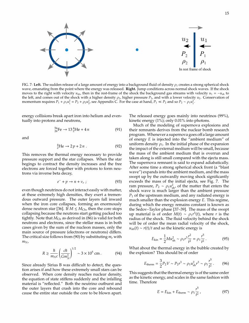
FIG. 7: Left. The sudden release of a large amount of energy into a background fluid of density ρ1 creates a strong spherical shockwave, emanating from the point where the energy was released. Right. Jump conditions across normal shock waves. If the shockmoves to the right with velocity ush, then in the rest-frame of the shock the background gas streams with velocity u1 = −ush tothe left, and comes out of the shock with a higher density ρ2, higher pressure P2, and with a lower velocity u2. Conservation ofmomentum requires P1 + ρ1u2

1 = P2 + ρ2u22, see Appendix C. For the case at hand, P1 P2 and so P2 ∼ ρ1u2

1.

energy collisions break apart iron into helium and even-tually into protons and neutrons,

5626Fe→ 13 4

2He + 4 n (91)

and

42He→ 2 p + 2 n . (92)

This removes the thermal energy necessary to providepressure support and the star collapses. When the starbegings to contract the density increases and the freeelectrons are forced together with protons to form neu-trons via inverse beta decay,

e− + p→ n + νe ; (93)

even though neutrinos do not interact easily with matter,at these extremely high densities, they exert a tremen-dous outward pressure. The outer layers fall inwardwhen the iron core collapses, forming an enormouslydense neutron star [36]. If M . MCh, then the core stopscollapsing because the neutrons start getting packed tootightly. Note that MCh as derived in (86) is valid for bothneutrons and electrons, since the stellar mass is in bothcases given by the sum of the nucleon masses, only themain source of pressure (electrons or neutrons) differs.The critical size follows from (90) by substituting me withmN,

R &

mNc

(c

Gm2N

)1/2

∼ 3 × 105 cm . (94)

Since already Sirius B was difficult to detect, the ques-tion arises if and how these extremely small stars can beobserved. When core density reaches nuclear density,the equation of state stiffens suddenly and the infallingmaterial is “reflected.” Both the neutrino outburst andthe outer layers that crash into the core and reboundcause the entire star outside the core to be blown apart.

The released energy goes mainly into neutrinos (99%),kinetic energy (1%); only 0.01% into photons.

Much of the modeling of supernova explosions andtheir remnants derives from the nuclear bomb researchprogram. Whenever a supernova goes off a large amountof energy E is injected into the “ambient medium” ofuniform density ρ1. In the initial phase of the expansionthe impact of the external medium will be small, becausethe mass of the ambient medium that is overrun andtaken along is still small compared with the ejecta mass.The supernova remnant is said to expand adiabatically.After some time a strong spherical shock front (a “blastwave”) expands into the ambient medium, and the massswept up by the outwardly moving shock significantlyexceeds the mass of the initial ejecta, see Fig. 7. Theram pressure, P2 ∼ ρ1u2

sh, of the matter that enters theshock wave is much larger than the ambient pressureP1 of the upstream medium, and any radiated energy ismuch smaller than the explosion energy E. This regime,during which the energy remains constant is known asthe Sedov–Taylor phase [37–39]. The mass of the sweptup material is of order M(t) ∼ ρ1r3(t), where r is theradius of the shock. The fluid velocity behind the shockwill be of order the mean radial velocity of the shock,ush(t) ∼ r(t)/t and so the kinetic energy is

Ekin =12

Mu2sh ∼ ρ1r3 r2

t2 = ρ1r5

t2 . (95)

What about the thermal energy in the bubble created bythe explosion? This should be of order

Etherm =32

P2V ∼ P2r3∼ ρ1u2

shr3∼ ρ1

r5

t2 . (96)

This suggests that the thermal energy is of the same orderas the kinetic energy, and scales in the same fashion withtime. Therefore

E = Ekin + Etherm ∼ ρ1r5

t2 , (97)

16

yielding

r(t) ∼(

Et2

ρ1

)1/5

. (98)

The expanding shock wave slows as it expands

ush =25

(Eρ1t3

)1/5

=25

(Eρ1

)1/2

r−3/2 . (99)

This means that the blask wave decelerates and dis-sapears after some time. The expanding supernovaremnant then passes from its Taylor-Sedov phase to its“snowplow” phase. During the snowplow phase, thematter of the ambient interstellar medium is swept upby the expanding dense shell, just as snow is swept upby a coasting snowplow.

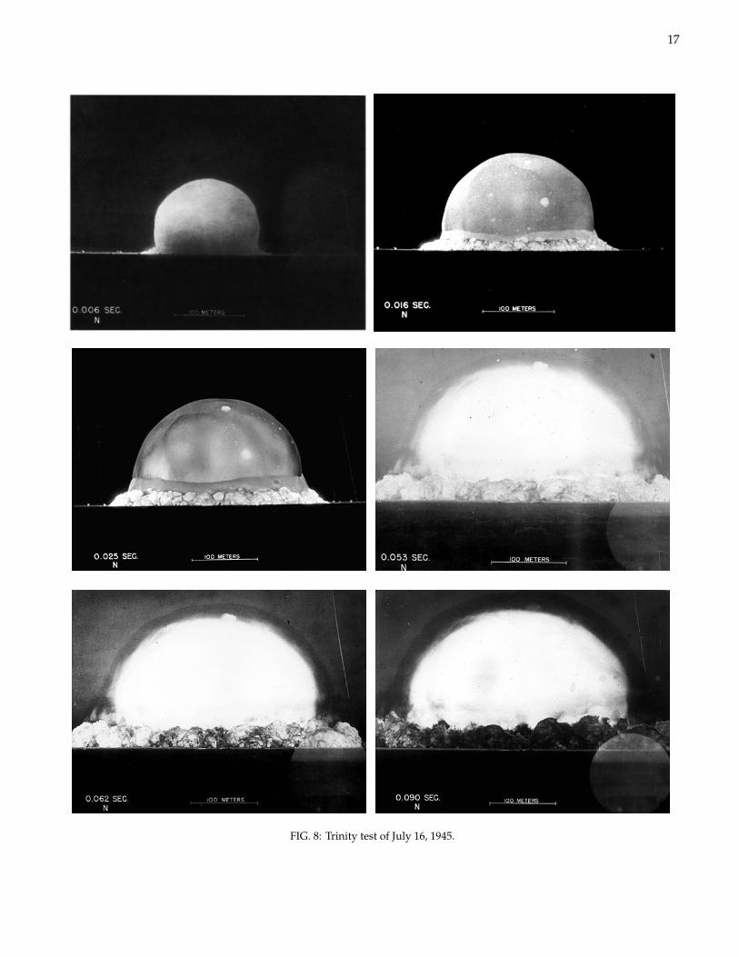
EXERCISE 4.6 Estimate the energy of the firstdetonation of a nuclear weapon (code name Trinity)from the time dependence of the radius of its shockwave. Photographs of the early stage of the explosionare shown in Fig. 8. The device was placed on the topof a tower, h = 30 m and the explosion took place atabout 1100 m above sea level. (i) Explain the originof the thin layer above the bright “fireball” that canbe seen in the last three pictures (t ≥ 0.053 s). Is theshock front behind or ahead of this layer? Read theradius of the shock front from the figures and plot itas a function of time after the explosion. The time andlength scale are indicated in the lables of the figures.(ii) Fit (by eye or numerical regression) a line to theradius vs. time dependence of the shock front in alog-log representation, ln(r) = a + b ln(t). Verifiy that b iscompatible with a Sedov-Taylor expansion. Then fix bto the theoretical expectation, re-evaluate a and estimatethe energy of the bomb in tons of TNT equivalent. [Hint:ignore the initial (short) phase of free expansion.]

If the final mass of a neutron star is less than MCh itssubsequent evolution is thought to be similar to that ofa white dwarf. In 1967, an unusual object emitting aradio signal with period T = 1.377 s was detected at theMullard Radio Astronomy Observatory. By its very na-ture the object was called “pulsar.” Only one year later,Gold argued that pulsars are rotating neutron stars [41].He predicted an increase on the pulsar period becauseof electromagnetic energy losses. The slow-down of theCrab pulsar was indeed discovered in 1969 [42].

If the mass of the neutron star is greater than MCh,then the star collapses under gravity, overcoming eventhe neutron exclusion principle [43]. The star eventuallycollapses to the point of zero volume and infinite density,creating what is known as a “singularity” [44–49]. As thedensity increases, the paths of light rays emitted fromthe star are bent and eventually wrapped irrevocablyaround the star. Any emitted photon is trapped intoan orbit by the intense gravitational field; it will never

leave it. Because no light escapes after the star reachesthis infinite density, it is called a black hole.

V. WARPING SPACETIME

A hunter is tracking a bear. Starting at his camp, hewalks one mile due south. Then the bear changes direc-tion and the hunter follows it due east. After one mile,the hunter loses the bear’s track. He turns north andwalks for another mile, at which point he arrives back athis camp. What was the color of the bear?

An odd question. Not only is the color of the bearunrelated to the rest of the question, but how can thehunter walk south, east and north, and then arrive backat his camp? This certainly does not work everywhereon Earth, but it does if you start at the North pole. There-fore the color of the bear has to be white. A surprisingobservation is that the triangle described by the hunter’spath has two right angles in the two bottom corners, andso the sum of all three angles is greater than 180. Thisimplies the metric space is curved.

What is meant by a curved space? Before answeringthis question, we recall that our normal method of view-ing the world is via Euclidean plane geometry, wherethe line element of the n-dimensional space is given by

ds2 =

n∑i=1

dx2i . (100)

Non-Euclidean geometries which involve curved spaceshave been independently imagined by Gauss [50],Bolyai [51], and Lobachevsky [52]. To understand theidea of a metric space herein we will greatly simplifythe discussion by considering only 2-dimensional sur-faces. For 2-dimensional metric spaces, the so-called firstand second fundamental forms of differential geometryuniquely determine how to measure lengths, areas andangles on a surface, and how to describe the shape of aparameterized surface.

A. 2-dimensional metric spaces

The parameterization of a surface maps points (u, v)in the domain to points ~σ(u, v) in space:

~σ(u, v) =

x(u, v)y(u, v)z(u, v)

. (101)

Differential geometry is the local analysis of how smallchanges in position (u, v) in the domain affect the positionon the surface ~σ(u, v), the first derivatives ~σu(u, v) and~σv(u, v), and the surface normal n(u, v).

The first derivatives, ~σu(u, v) and ~σv(u, v), are vectorsthat span the tangent plane to the surface at point ~σ(u, v).The surface normal at point~σ is defined as the unit vector

17

Figures also available at http://cosmo.nyu.edu/~mu495/HEA15/trinity/

2

FIG. 8: Trinity test of July 16, 1945.

18

normal to the tangent plane at point ~σ and is computedusing the cross product of the partial derivatives of thesurface parameterization,

n(~σ) =~σu × ~σv

||~σu × ~σv||. (102)

The tangent vectors and the surface normal define anorthogonal coordinate system at point ~σ(u, v) on the sur-face, which is the framework for describing the localshape of the surface.

Geometrically, d~σ is a differential vector quantity thatis tangent to the surface in the direction defined by duand dv. The first fundamental form, I, which measuresthe distance of neighboring points on the surface withparameters (u, v) and (u+du, v+dv), is given by the innerproduct of d~σ with itself

I ≡ ds2 = d~σ · d~σ = (~σudu + ~σvdv) · (~σudu + ~σvdv)= (~σu · ~σu)du2 + 2(~σu · ~σv)dudv + (~σv · ~σv)dv2

= Edu2 + 2Fdudv + Gdv2 , (103)

where E, F and G are the first fundamental coefficients.The coefficients have some remarkable properties. Forexample, they can be used to calculate the surface area.Namely, the area bounded by four vertices ~σ(u, v), ~σ(u +δu, v), ~σ(u, v + δv), ~σ(u + δu, v + δv) can be expressed interms of the first fundamental form with the assistanceof Lagrange identity

n−1∑i=1

n∑j=i+1

(aib j − a jbi)2 =

n∑k=1

a2k

n∑

k=1

b2k

−

n∑k=1

akbk

2

, (104)

which applies to any two sets a1, a2, · · · , an andb1, b2, · · · , bn of real numbers. The classical area ele-ment is found to be

δA = |~σu δu × ~σv δv| =√

EG − F2 δu δv , (105)

or in differential form

dA =√

EG − F2 du dv . (106)

Note that the expression under the square root in (106)is precisely |~σu × ~σv| and so it is strictly positive at theregular points.

The key to the second fundamental form, II, is theunit normal vector. The second fundamental form coef-ficients at a given point in the parametric uv-plane aregiven by the projections of the second partial deriva-tives of ~σ at that point onto the normal vector and canbe computed with the aid of the dot product as follows:e = ~σuu · n, f = ~σuv · n, and g = ~σvv · n. The secondfundamental form,

II = e du2 + 2 f du dv + g dv2 , (107)

can be used to characterize the local shape of the foldedsurface.

The concept of curvature, while intuitive for a planecurve (the reciprocal of the radius of curvature), requiresa more comprehensive definition for a surface. Througha point on a surface any number of curves may be drawnwith each having a different curvature at the point. Wehave seen that at any point on a surface we can find nwhich is at right angles to the surface; planes containingthe normal vector are called normal planes. The inter-section of a normal plane and the surface will form acurve called a normal section and the curvature of thiscurve is the normal curvature κ. For most points onmost surfaces, different sections will have different cur-vatures; the minimum and maximum values of these arecalled the principal curvatures, denoted by κ1 and κ2.The Gaussian curvature is defined by the product of thetwo principal curvatures K = κ1κ2. It may be calculatedusing the first and second fundamental coefficients. Ateach grid point where these values are known two ma-trices are defined. The matrix of the first fundamentalform,

I =

(E FF G

), (108)

and the matrix of the second fundamental form,

II =

(e ff g

). (109)

The Gaussian curvature is given by

K =det IIdet I

. (110)

As an illustration, consier a half-cylinder of radius Roriented along the x axis. At a particular point on thesurface, the scalar curvature can have different valuesdepending on direction. In the direction of the half-cylinder’s axis (parallel to the x axis), the surface has zeroscalar curvature, κ = 0. This is the smallest curvaturevalue at any point on the surface, and therefore κ1 is inthis direction. For a curve on the half-cylinder’s surfaceparallel to the (y, z) plane, the cylinder has uniform scalarcurvature. In fact this curvature is the greatest possibleon the surface, so that κ2 = 1/R is in this direction. Fora curve on the surface not in one of these directions, thescalar curvature is greater than κ1 and less than κ2. TheGaussian curvature is K = 0.

2-dimensional metric spaces can be classified accord-ing to the Gaussian curvature into elliptic (K > 0), flat(K = 0), and hyperbolic (K < 0). Triangles which lie onthe surface of an elliptic geometry will have a sum ofangles which is greater than 180. Triangles which lieon the surface of an hyperbolic geometry will have asum of angles which is less than 180.

19

EXERCISE 5.1 The unit sphere can be parametrizedas

~σ(u, v) =

cos u sin vsin u sin v

cos v

(111)

where (u, v) ∈ [0, 2π) × [0, π]. (i) Find the distance ofneighboring points on the surface with parameters (u, v)and (u + du, v + dv), a.k.a. the line element ds2. (ii) Findthe surface area. (iii) Find the Gaussian curvature.

EXERCISE 5.2 The tractrix is a curve with the follow-ing nice interpretation: Suppose a dog-owner takes hispet along as he goes for a walk “down” the y-axis. Hestarts from the origin, with his dog initially standing onthe x-axis at a distance r away from the owner. Thenthe tractrix is the path followed by the dog if he “fol-lows his owner unwillingly”, i.e., if he constantly pullsagainst the leash, keeping it tight. This means mathe-matically that the leash is always tangent to the path ofthe dog, so that the length of the tangent segment fromthe tractrix to the y-axis has constant length r. The trac-trix has a well-known surface of revolution called thepseudosphere which, for r = 1, can be parametrized as

~σ(u, v) =

sechu cos vsechu sin vu − tanhu

, (112)

with u ∈ (−∞,∞) and v ∈ [0, 2π). (i) Find the lineelement. (ii) Find the surface area. (iii) Find theGaussian curvature.

A curve γwith parametr t on a surface ~σ(u, v) is calleda geodesic if at every point γ(t) the acceleration vector~γ(t) is either zero or parallel to its unit normal n.

EXERCISE 5.3 Show that a geodesic γ(t) on a surface~σ has constant speed.

EXERCISE 5.4 A curve γ on a surface ~σ is a geodesicif and only if for any part γ(t) = ~σ(u(t), v(t)) containedin a surface patch ~σ, the following two equations aresatisfied:

ddt

(Eu + Fv) =12

(Euu2 + 2Fuuv + Guv2) , (113)

ddt

(Fu + Gv) =12

(Evu2 + 2Fvuv + Gvv2) , (114)

where Edu2 +2Fdudv+Gdv2 is the first fundamental formof ~σ. (113) and (114) are called the geodesic equations.They are nonlinear and solvable analytically on rareoccasions only.

EXERCISE 5.5 Show that if γ is a geodesic on the unitsphere S2, then γ is part of a great circle. Consider the

patch under the parametrization

~σ(θ, φ) =

cosθ cosφcosθ sinφ

sinθ

. (115)

[Hint: A great circle (a.k.a. orthodrome) of a sphere isthe intersection of the sphere and a plane which passesthrough the center point of the sphere.]

The scalar curvature (or Ricci scalar) is the simplestcurvature invariant of an n-dimensional hypersurface.To each point on the hypersurface, it assigns a singlereal number determined by the intrinsic geometry ofthe hypersurface near that point. It provides one way ofmeasuring the degree to which the geometry determinedby a given metric might differ from that of ordinary Eu-clidean n-space. In two dimensions, the scalar curvatureis twice the Gaussian curvature, R = 2K, and completelycharacterizes the curvature of a surface. In more thantwo dimensions, however, the curvature of hypersur-faces involves more than one functionally independentquantity.

B. Schwarzschild metric

Consider a freely falling spacecraft in the gravitationalfield of a radially symmetric mass distribution with totalmass M. Because the spacecraft is freely falling, no ef-fects of gravity are felt inside. Then, the spacetime coor-dinates from r→∞ should be valid inside the spacecraft.Let us call these coordinates ~Σ∞(t∞, x∞, y∞, z∞), with x∞parallel and y∞, z∞ transversal to movement. The space-craft has velocity v at the distance r from the mass M,measured in the coordinate system ~Σ = (t, r, θ, φ) inwhich the mass M is at rest at r = 0. As long as thegravitational field is weak, to first order approximationthat the laws of special relativity hold [58], and we canuse a Lorentz transformation [26] to relate ~Σ at rest and~Σ∞ moving with v = βc. We will define shortly what“weak” means in this context. For the moment, we pre-sume that effects of gravity are small if the velocity ofthe spacecraft, which was at rest a r → ∞, is still smallv c. Should this be the case, we have

dt∞ = dt√

1 − β2

dx∞ =dr√

1 − β2

dy∞ = r dθdz∞ = r sinθ dφ . (116)

The infinitesimal distance between two spacetime eventsis given by the Minkowskian line element [59]

ds2 = gµνdxµdxν = c2dt2∞ − dx2

∞ − dy2∞ − dz2

∞ , (117)

20

which, for the case at hand, becomes

ds2 = (1 − β2)c2dt2−

dr2

1 − β2 + r2(dθ2 + sin2 dφ2) . (118)

Herein we follow the notation of [27]: Greek indices(µ, ν, · · · ) run from 0 to 3 and Latin indices (i, j, · · · ) from1 to 3.

We now turn to determine β from measurable quanti-ties of the system: M and r. Consider the energy of thespacecraft with rest mass m,

(γ − 1)mc2−

GγmMr

= 0 , (119)

where the first term is the kinetic energy and the sec-ond the Newtonian expression for the potential energy.Note that here we have made the crucial assumption thatgravity couples not only to the mass of the spacecraft butalso to its total energy. Dividing by γmc2 gives(

1 −1γ

)−

GMrc2 = 0 . (120)

Introducing α = GM/c2 we can re-write (120) as√1 − β2 = 1 −

αr, (121)

where γ = (1 − β2)−1/2. (121) leads to

1 − β2 = 1 −2αr

+α2

r2 ≈ 1 −2αr

; (122)

in the last step, we neglected the term (α/r)2, since weattempt only at an approximation for large distances,where gravity is still weak. Inserting this expression into(118), we obtain the metric describing the gravitationalfield produced by a radially symmetric mass distribu-tion,

ds2 =(1 −

2αr

)c2dt2

−

(1 −

2αr

)−1

dr2− r2dΩ2 , (123)

where dΩ2 = dθ2 + sin2 θdφ2. Wickedly, this agrees withthe exact result found by Schwarzschild [60] by solv-ing Einstein’s vacuum field equations of general relativ-ity [61].

As in special relativity, the line element ds2 determinesthe time and spatial distance between two spacetimeevents. The time measured by an observer in the instan-taneous rest frame, known as the proper time dτ, is givenby dτ = ds/c [27]. In particular, the time difference be-tween two events at the same point is obtained by settingdxi = 0. If we choose two static observers at the positionr and r′, then we find with dr = dφ = dθ = 0,

dτ(r)dτ(r′)

=

√g00(r) dt√g00(r′) dt

=

√g00(r)g00(r′)

. (124)

The time intervals dτ(r′) and dτ(r) are different and thusthe time measured by clocks at different distances r fromthe mass M will differ too. In particular, the time τ∞measured by an observer at infinity will pass faster thanthe time experienced in a gravitational field,

τ∞ =τ(r)

√1 − 2α/r

< τ(r) . (125)

Since frequencies are inversely proportional to time, thefrequency or energy of a photon traveling from r to r′will be affected by the gravitational field as

ν(r′)ν(r)

=

√1 − 2α/r1 − 2αr′

. (126)

Therefore, an observer at r′ → ∞ will receive photons,which were emitted with frquency ν by a source at posi-tion r, redhsifted to frequency ν∞,

ν∞ =

√1 −

2GMrc2 ν(r) . (127)

Note that the photon frequency is redshifted by the grav-itational field. The size of this effect is of order Φ/c2,where Φ = −GM/r is the Newtonian gravitational po-tential. We are now in position to specify more pre-cisely what weak gravitational fields means. As long as|Φ|/c2

1, the deviation of

g00 = 1 −2GMrc2 ≈ 1 − 2

Φ(r)c2 (128)

from the Minkowski value g00 = 1 is small, and Newto-nian gravity is a sufficient approximation.

What is the meaning of r = 2α? At

RSch =2GM

c2 = 3 kmM

M, (129)

the Schwarzschild coordinate system (123) becomes ill-defined. However, this does not mean necessarily that atr = RSch physical quantities like tidal forces become in-finite. As a matter of fact, all scalar invariants are finite,e.g. R = 0 and K = 12RSch/r6. Here R is the Ricci scalarand K the Kretschmann scalar [62], a quadratic scalar in-variant used to find the true singularities of a spacetime.The Schwarzschild’s scalar invariants can only be foundby long and troublesome calculation that is beyond thescope of this course; for a comprehensive discussion seee.g. [63, 64]. Before proceeding we emphasize again that,whether or not the singularity is moved to the origin,only depends on the coordinate frame used, and has nophysical significance whatsoever; see Appendix D for anexample.

If the gravitating mass is concentrated inside a radiussmaller than RSch then we cannot obtain any informationabout what is going on inside RSch, and we say r = RSchdefines an event horizon. An object smaller than its

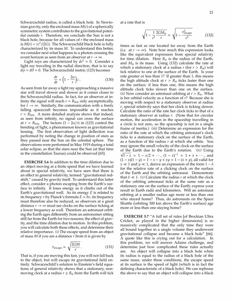
21

Schwarzschild radius, is called a black hole. In Newto-nian gravity, only the enclosed mass M(r) of a sphericallysymmetric system contributes to the gravitational poten-tial outside r. Therefore, we conclude the Sun is not ablack hole, becasue for all values of r the enclosed massis M(r) < rc2/(2G). The Schwarzschild black hole is fullycharacterized by its mass M. To understand this better,we consider next what happens to a photon crossing theevent horizon as seen from an observer at r→∞.

Light rays are characterized by ds2 = 0. Consider alight ray traveling in the radial direction, that is to saydφ = dθ = 0. The Schwarzschild metric (123) becomes

drdt

=(1 −

2αr

)c . (130)

As seen from far away a light ray approaching a massivestar will travel slower and slower as it comes closer tothe Schwarzschild radius. In fact, for an observer at in-finity the signal will reach r = RSch only asymptotically,for t → ∞. Similarly, the communication with a freelyfalling spacecraft becomes impossible as it reachesr = RSch. A more detailed analysis shows that indeed,as seen from infinity, no signal can cross the surfaceat r = RSch. The factors (1 − 2α/r) in (123) control thebending of light, a phenomenon known as gravitationallensing. The first observation of light deflection wasperformed by noting the change in position of stars asthey passed near the Sun on the celestial sphere. Theobservations were performed in May 1919 during a totalsolar eclipse, so that the stars near the Sun (at that timein the constellation Taurus) could be observed [65].

EXERCISE 5.6 In addition to the time dilation due toan object moving at a finite speed that we have learnedabout in special relativity, we have seen that there isan effect in general relativity, termed “gravitational red-shift,” caused by gravity itself. To understand this lattereffect, consider a photon escaping from the Earth’s sur-face to infinity. It loses energy as it climbs out of theEarth’s gravitational well. As its energy E is related toits frequency ν by Planck’s formula E = hν, its frequencymust therefore also be reduced, so observers at a greatdistance r→∞must see clocks on the surface ticking ata lower frequency as well. Therefore an astronaut orbit-ing the Earth ages differently from an astronomer sittingstill far from the Earth for two reasons; the effect of grav-ity, and the time dilation due to motion. In this problem,you will calculate both these effects, and determine theirrelative importance. (i) The escape speed from an objectof mass M if you are a distance r from it is given by

vescape =

√2GM

r. (131)

That is, if you are moving this fast, you will not fall backto the object, but will escape its gravitational field en-tirely. Schwarzschild’s solution to Einstein’s field equa-tions of general relativity shows that a stationary, non-moving clock at a radius r ≥ R⊕ from the Earth will tick

at a rate that is√1 −

1c2

2GM⊕r

=

√1 −

v2escape

c2 (132)

times as fast as one located far away from the Earth(i.e. at r → ∞). Note how much this expression lookslike the equivalent expression from special relativityfor time dilation. Here R⊕ is the radius of the Earth,and M⊕ is its mass. Using (132) calculate the rate atwhich a stationary clock at a radius r (for r > R⊕) willtick relative to one at the surface of the Earth. Is yourrate greater or less than 1? If greater than 1, this meansthe high altitude clock at r > R⊕ ticks faster than oneon the surface; if less than one, this means the highaltitude clock ticks slower than one on the surface.(ii) Now consider an astronaut orbiting at r > R⊕. Whatis her orbital velocity as a function of r? Because she ismoving with respect to a stationary observer at radiusr, special relativity says that her clock is ticking slower.Calculate the ratio of the rate her clock ticks to that of astationary observer at radius r. (Note that for circularmotion, the acceleration in the spaceship travelling ina circle is not zero, so the spaceship is not in a singleframe of inertia.) (iii) Determine an expression for theratio of the rate at which the orbiting astronaut’s clockticks to a stationary clock on the surface of the Earth,as a function of the radius r at which she orbits. Youmay ignore the small velocity of the clock on the surfaceof the Earth due to the Earth’s rotation. (iv) Using√

1 − x ≈ 1 − x/2 + · · · , (1 − x)−1≈ 1 + x + · · · , and

(1 − x)(1 − y) = 1 − x − y + xy ≈ 1 − (x + y), all valid forx 1 and y 1, derive an expression of the form 1 − δfor the relative rate of a clicking clock on the surfaceof the Earth and the orbiting astronaut. Demonstratethat δ 1. (v) Calculate the radius r at which the clockof the orbiting astronaut ticks at the same rate as astationary one on the surface of the Earth; express yourresult in Earth radii and kilometers. Will an astronautorbiting at a smaller radius age more or less than onewho stayed home? Thus, do astronauts on the SpaceShuttle (orbiting 300 km above the Earth’s surface) agemore or less than one staying home?

EXERCISE 5.7 “A full set of rules [of Brockian UltraCricket, as played in the higher dimensions] is somassively complicated that the only time they wereall bound together in a single volume they underwentgravitational collapse and became a black hole” [66].A quote like this is crying out for a calculation. Inthis problem, we will answer Adams challenge, anddetermine just how complicated these rules actuallyare. An object will collapse into a black hole whenits radius is equal to the radius of a black hole of thesame mass; under these conditions, the escape speedat its surface is the speed of light (which is in fact thedefining characteristic of a black hole). We can rephrasethe above to say that an object will collapse into a black

22

hole when its density is equal to the density of a blackhole of the same mass. (i) Derive an expression for thedensity of a black hole of mass M. Treat the volumeof the black hole as the volume of a sphere of radiusgiven by the Schwarzschild radius. As the mass of ablack hole gets larger, does the density grow or shrink?(ii) Determine the density of the paper making up theCricket rule book, in units of kilograms per cubic meter.Standard paper has a surface density of 75 g per squaremeter, and a thickness of 0.1 mm. (iii) Calculate themass (in solar masses), and radius (in AU) of the blackhole with density equal to that of paper. (iv) How manypages long is the Brockian Ultra Cricket rule book?Assume the pages are standard size (8.5′′ × 11′′). Forcalculational simplicity, treat the book as spherical (acommon approximation in this kind of problem). Whatif the rule book were even longer than you have justcalculated? Would it still collapse into a black hole?

EXERCISE 5.8 Black holes provide the ultimate lab-oratory for studying strong-field gravitational physics.The tides near black holes can be so extreme that aprocess informally called “spaghettification” occurs inwhich a body falling towards a black hole is stronglystretched due to the difference in gravitational force atdifferent locations along the body (this is called a tidaleffect). In the following, imagine that you are fallinginto a 3M black hole. (i) What is the Schwarzschildradius of this black hole (in km)? (ii) You are 1.5 m talland 70 kg in mass and are falling feet first. At whatdistance from the black hole would the gravitationalforce on your feet exceed the gravitational force on yourhead by 10 kN? Express this distance in km and inSchwarzschild radii of the black hole. (iii) To appreciateif this amount of force is enough to “spaghettify” andkill you, imagine that you are suspended from a ceilingof your room (on Earth) with a steel plate tied to yourfeet. Calculate the mass of the plate (in kg) that willgive you a nice tug of 10 kN (you can ignore the weightof your body here). Do you think this pull will killyou? (iv) Now consider a trip toward the supermassiveblack hole at the center of our Galaxy, which has anestimated mass of 4 million M. How does this changethe distance at which you will be “spaghettified” by thedifferential gravity force of 10 kN? Express your answerin km and in Schwarzschild radii of the black hole.(v) Find the smallest mass of the black hole for whichyou would not die by “spaghettification” before fallingwithin its event horizon.

EXERCISE 5.9 In the Schwarzschild metric r is a co-moving coordinate, not a real physical distance. Rather,integrals over ds constitute physical distances. In the fol-lowing we will take slices of spacetime at a constant time(dt = 0). (i) Compute the physical circumference, C, ata given coordinate distance R from the center of a blackhole of mass M at θ = π/2. (ii) Compute the physicaldistance Rphys from the center of the black hole out to

the coordinate distance R (assume R > RSch and take theabsolute value of grr). [Hint: The following facts may behelpfull: ∫ 1

0

√ξ

1 − ξdξ =

π2, (133)

and∫ α

1

√ξ

1 − ξdξ = ln(

√

α − 1 +√α) +

√

α − 1√α , (134)

where α > 1 is constant.] (iii) Now use your answers topart (i) and part (ii) to compute Π where C = 2ΠRphys.(iv) Plot Π as a function of ξ ≡ R/RSch for ξ ∈ [1, 103] (uselog axes for the x axis). What happens with Π as ξ→∞?

C. Eddington luminosity and black hole growth

Binary X-ray sources are places to find strong blackhole candidates [67, 68]. A companion star is a perfectsource of infalling material for a black hole. As the matterfalls or is pulled towards the black hole, it gains kineticenergy, heats up and is squeezed by tidal forces. Theheating ionizes the atoms, and when the atoms reach afew million degrees Kelvin, they emit X-rays. The X-rays are sent off into space before the matter crosses theevent horizon, and so we can detect this X-ray emission.Another sign of the presence of a black hole is randomvariation of emitted X-rays. The infalling matter thatemits X-rays does not fall into the black hole at a steadyrate, but rather more sporadically, which causes an ob-servable variation in X-ray intensity. Additionally, if theX-ray source is in a binary system, the X-rays will beperiodically cut off as the source is eclipsed by the com-panion star.

Cygnus X-1 is one of the strongest X-ray sources wecan detect from Earth [69] and the first widely thought tobe a black hole, after the detection of its rapid X-ray vari-ability [70] and the identification of its optical countem-part with the blue supergiant star HDE 226868 [71, 72].The X-ray emission is powered mainly by accretion fromthe strong stellar wind from HDE 226868 [73]. While thedisk of accreting matter is incredibly bright on its own,Cygnus X-1 has another source of light: a pair of jets per-pendicular to the disk erupt from the black hole carryingpart of the infalling material away into the interstellarspace [74].

Consider a steady spherically symmetrical accretion.We assume the accreting material to be mainly hydro-gen and to be fully ionized. Under these circumstances,the radiation exerts a force mainly on the free electronsthrough Thomson scattering, since the scattering crosssection for protons is a factor (me/mp)2 smaller, whereme/mp = 5 × 10−4 is the ratio of the electron and protonmasses [75]. If F is the radiant energy flux (erg s−1cm−2)and σT = 6.7 × 10−25 cm2 is the Thomson cross section,

23

then the outward radial force on each electron equals therate at which it absorbs momentum,

Fout =σTF

c. (135)

The attractive electrostatic Coulomb force between theelectrons and protons means that as they move out theelectrons drag the protons with them. In effect, the radi-ation pushes out electron-proton pairs against the totalgravitational force

Fin =GMr2 (mp + me) (136)

acting on each pair at a radial distance r from the center.If the luminosity of the accreting source is L (erg s−1), wehave

F =L

4πr2 (137)

by spherical symmetry, so the net inward force on anelectron-proton pair is

Fnet =(GMmp −

LσT

4πc

) 1r2 . (138)

There is a limiting luminosity for which this expressionvanishes, called the Eddington limit [76]

LEdd =4πGMmp

σT' 1.3 × 1038

(M

M

)erg s−1 . (139)

At greater luminosities the outward pressure of radiationwould exceed the inward gravitational attraction andaccretion would be halted.

Active galactic nuclei (AGNs) are galaxies thatharbor compact masses at the center exhibiting intensenon-thermal emission that is often variable, whichindicates small sizes (light months to light years). Theluminosity of an accreting black hole is proportional tothe rate at which it is gaining mass. Under favorableconditions, the accretion leads to the formation of ahighly relativistic collimated jet. The formation of thejet is not well constrained, but it is thought to changefrom magnetic-field-dominated near the central engineto particle (electron and positron, or ions and electrons)dominated beyond pc distances. The AGN taxonomy,controlled by the dichotomy between radio-quiet andradio-loud classes, is represented in Fig. 9. The appear-ance of an AGN depends crucially on the orientationof the observer with respect to the symmetry axis ofthe accretion disk [78]. In this scheme, the differencebetween radio-loud and radio-quiet AGN depends onthe presence or absence of radio-emitting jets poweredby the central nucleus, which in turn may be speculatedto depend on: (i) black hole rotation; (ii) low power orhigh power, as determined by the mass-accretion rateMc2/LEdd [79].

EXERCISE 5.10 The pictures in Fig. 10 show a timesequence of radio observations of the quasar 0827+243.The core of the quasar is the bright object at a distanceof 0 ly and a fainter blob of plasma is moving awayfrom it. (i) What is the apparent velocity of the motionof the plasma blob? (ii) Derive the apparent transversevelocity of an object ejected from a source at velocity v atan angle θ with respect to the line of sight between thesource and the observer. (iii) Which angle maximizesthe apparent transverse velocity? What is accordinglythe minimal Lorentz-factor of the plasma blob observedin 0827+243?

VI. EXPANSION OF THE UNIVERSE

The observations that we will discuss in this sectionreveal that the universe is in a state of violent explosion,in which the galaxies are rushing appart at speeds ap-proaching the speed of light. Moreover, we can extrapo-late this explosion backwards in time and conclude thatall the galaxies must have been much closer at the sametime in the past – so close, in fact, that neither galaxiesnor stars nor even atoms or atomic nuclei could havehad a separate existence.

A. Hubble’s law

The XVI century finally saw what came to be a water-shed in the development of Cosmology. In 1543 Coper-nicus published his treatise “De Revolutionibus OrbiumCelestium” (The Revolution of Celestial Spheres) wherea new view of the world is presented: the heliocentricmodel [3].

It is hard to underestimate the importance of this work:it challenged the age long views of the way the uni-verse worked and the preponderance of the Earth and,by extension, of human beings. The realization thatwe, our planet, and indeed our solar system (and evenour Galaxy) are quite common in the heavens and re-produced by myriads of planetary systems, provided asobering (though unsettling) view of the universe. Allthe reassurances of the cosmology of the Middle Ageswere gone, and a new view of the world, less secure andcomfortable, came into being. Despite these “problems”and the many critics the model attracted, the systemwas soon accepted by the best minds of the time such asGalileo.

The simplest and most ancient of all astronomical ob-servations is that the sky grows dark when the Sun goesdown. This fact was first noted by Kepler, who, in theXVII century, used it as evidence for a finite universe. Inthe XIX century, when the idea of an unending, unchang-ing space filled with stars like the Sun was widspreadin consequence of the Copernican revolution, the ques-tion of the dark night sky became a problem. To clearlyascertain this problem, we recall that if absorption is

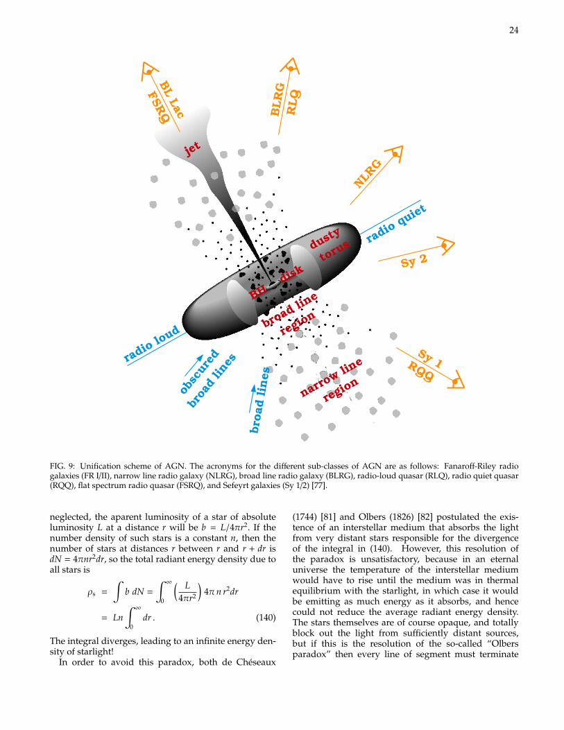
24

1.1. QUASARS, AGN AND BLAZARS 27

added: a dusty torus or a wrapped disk obscuring the light of type 2objects.

The unification scheme that has emerged combining these ingredi-ents (black hole, disk, jet, torus and clouds) is usually attributed toAntonucci (1993) and Urry & Padovani (1995). As shown in Fig. 6, itis based on orientation effects compared to the line of sight.

Figure 6. Unification scheme of AGN. The acronymsfor the different sub-classes of AGN are given in Fig. 2.Adapted from Urry & Padovani (1995) .

past

el-0

0822

242,

ver

sion

1 -

14 M

ay 2

013

FIG. 9: Unification scheme of AGN. The acronyms for the different sub-classes of AGN are as follows: Fanaroff-Riley radiogalaxies (FR I/II), narrow line radio galaxy (NLRG), broad line radio galaxy (BLRG), radio-loud quasar (RLQ), radio quiet quasar(RQQ), flat spectrum radio quasar (FSRQ), and Sefeyrt galaxies (Sy 1/2) [77].

neglected, the aparent luminosity of a star of absoluteluminosity L at a distance r will be b = L/4πr2. If thenumber density of such stars is a constant n, then thenumber of stars at distances r between r and r + dr isdN = 4πnr2dr, so the total radiant energy density due toall stars is

ρs =

∫b dN =

∫∞

0

( L4πr2

)4πn r2dr

= Ln∫∞

0dr . (140)

The integral diverges, leading to an infinite energy den-sity of starlight!

In order to avoid this paradox, both de Cheseaux

(1744) [81] and Olbers (1826) [82] postulated the exis-tence of an interstellar medium that absorbs the lightfrom very distant stars responsible for the divergenceof the integral in (140). However, this resolution ofthe paradox is unsatisfactory, because in an eternaluniverse the temperature of the interstellar mediumwould have to rise until the medium was in thermalequilibrium with the starlight, in which case it wouldbe emitting as much energy as it absorbs, and hencecould not reduce the average radiant energy density.The stars themselves are of course opaque, and totallyblock out the light from sufficiently distant sources,but if this is the resolution of the so-called “Olbersparadox” then every line of segment must terminate

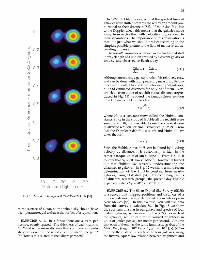
25

for component C2 in 0827+243, however, has been establishedwith a high degree of confidence.

4. DISCUSSION

Inspection of Table 3 shows that different Gaussian compo-nents in the same source have different apparent speeds. Thereare two possible origins of these different apparent speeds. Thefirst possibility is that the components move with different pat-tern speeds that are not necessarily equal to the bulk speed. Lister(2006) concluded from a correlation of apparent speeds fromthe 2 cm andMOJAVE surveys with other source properties thatvarious pattern speeds are present in the jets, but that the fastest

Fig. 5.—Distances from the core of Gaussian component centers as a functionof time. The lines are the least-squares fits to outward motion with constant speed.

Fig. 6.—Mosaic of images of 0827+243 at 22 GHz. The bright feature movesapproximately 15 lt-yr in 0.6 yr (source frame), for an apparent speed of about25c. Only four of the six epochs are shown to prevent overlapping of images.The peak flux densities at the four epochs are 1.2, 1.6, 1.2, and 1.1 Jy beam!1,respectively. Images have been rotated 25" clockwise and restored with a cir-cular 0.5 mas beam. Model component C3 is at the center of the bright jetfeature.

PINER ET AL.202 Vol. 640

FIG. 10: Mosaic of images of 0827+243 at 22 GHz [80].

at the surface of a star, so the whole sky should havea temperature equal to that at the surface of a typical star.

EXERCISE 6.1 (i) In a forest there are n trees perhectare, evenly spaced. The thickness of each trunk isD. What is the mean distance that you have an unob-structed view into the woods, i.e. the mean free path?(ii) How is this related to the Olbers paradox?

In 1929, Hubble discovered that the spectral lines ofgalaxies were shifted towards the red by an amount pro-portional to their distances [83]. If the redshift is dueto the Doppler effect, this means that the galaxies moveaway from each other with velocities proportional totheir separations. The importance of this observation isthat it is just what we should predict according to thesimplest possible picture of the flow of matter in an ex-panding universe.

The redshift parameter is defined as the traditional shiftin wavelength of a photon emitted by a distant galaxy attime tem and observed on Earth today

z =λobs

λem− 1 =

νem

νobs− 1, (141)

Although measuring a galaxy’s redshift is relatively easy,and can be done with high precision, measuring its dis-tance is difficult. Hubble knew z for nearly 50 galaxies,but had estimated distances for only 20 of them. Nev-ertheless, from a plot of redshift versus distance (repro-duced in Fig. 11) he found the famous linear relationnow known as the Hubble’s law:

z =H0

cr , (142)

where H0 is a constant (now called the Hubble con-stant). Since in the study of Hubble all the redshift weresmall, z < 0.04, he was able to use the classical non-relativistic realtion for small velocities (v c). From(48) the Doppler redshift is z ≈ v/c and Hubble’s lawtakes the form

v = H0 r . (143)

Since the Hubble constant H0 can be found by dividingvelocity by distance, it is customarily written in therather baroque units of km s−1 Mpc−1. From Fig. 11 itfollows that H0 = 500 km s−1 Mpc−1. However, it turnedout that Hubble was severely underestimating thedistances to galaxies. In Fig. 12 we show a more recentdetermination of the Hubble constant from nearbygalaxies, using HST data [84]. By combining resultsof different research groups, the present day Hubbleexpansion rate is H0 = 70+5

−3 km s−1 Mpc−1.

EXERCISE 6.2 The Sloan Digital Sky Survey (SDSS)is a survey that mapped positions and distances of amillion galaxies using a dedicated 2.5 m telescope inNew Mexico [85]. In this exercise, you will use datafrom this survey to calculate H0. In Fig. 13 we showthe spectrum of a star in our galaxy and spectra of fourdistant galaxies, as measured by the SDSS. For each ofthe galaxies, we indicate the measured brightness inunits of Joules per square meter per second. Assumethat each of them has the same luminosity as that of theMilky Way (LMW = 1011 L, or LMW = 4×1037 J/s). (i) De-termine the distance to each of the four galaxies, usingthe inverse-square law relation between brightness and

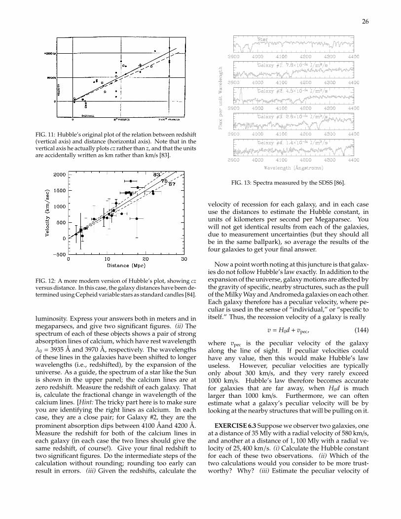
26

16 CHAPTER 2. FUNDAMENTAL OBSERVATIONS

Figure 2.4: Edwin Hubble’s original plot of the relation between redshift(vertical axis) and distance (horizontal axis). Note that the vertical axisactually plots cz rather than z – and that the units are accidentally writtenas km rather than km/s. (from Hubble 1929, Proc. Nat. Acad. Sci., 15,168)

FIG. 11: Hubble’s original plot of the relation between redshift(vertical axis) and distance (horizontal axis). Note that in thevertical axis he actually plots cz rather than z, and that the unitsare accidentally written as km rather than km/s [83].2.3. REDSHIFT PROPORTIONAL TO DISTANCE 17

Figure 2.5: A more modern version of Hubble’s plot, showing cz versusdistance. In this case, the galaxy distances have been determined usingCepheid variable stars as standard candles, as described in Chapter 6. (fromFreedman, et al. 2001, ApJ, 553, 47)

velocity away from Earth. Since the values of z in Hubble’s analysis were allsmall (z < 0.04), he was able to use the classical, nonrelativistic relation forthe Doppler shift, z = v/c, where v is the radial velocity of the light source(in this case, a galaxy). Interpreting the redshifts as Doppler shifts, Hubble’slaw takes the form

v = H0r . (2.6)

Since the Hubble constant H0 can be found by dividing velocity by distance,it is customarily written in the rather baroque units of km s−1 Mpc−1. WhenHubble first discovered Hubble’s Law, he thought that the numerical value ofthe Hubble constant was H0 = 500 km s−1 Mpc−1 (see Figure 2.4). However,it turned out that Hubble was severely underestimating the distances togalaxies.

Figure 2.5 shows a more recent determination of the Hubble constantfrom nearby galaxies, using data obtained by (appropriately enough) the

FIG. 12: A more modern version of Hubble’s plot, showing czversus distance. In this case, the galaxy distances have been de-termined using Cepheid variable stars as standard candles [84].

luminosity. Express your answers both in meters and inmegaparsecs, and give two significant figures. (ii) Thespectrum of each of these objects shows a pair of strongabsorption lines of calcium, which have rest wavelengthλ0 = 3935 Å and 3970 Å, respectively. The wavelengthsof these lines in the galaxies have been shifted to longerwavelengths (i.e., redshifted), by the expansion of theuniverse. As a guide, the spectrum of a star like the Sunis shown in the upper panel; the calcium lines are atzero redshift. Measure the redshift of each galaxy. Thatis, calculate the fractional change in wavelength of thecalcium lines. [Hint: The tricky part here is to make sureyou are identifying the right lines as calcium. In eachcase, they are a close pair; for Galaxy #2, they are theprominent absorption dips between 4100 Åand 4200 Å.Measure the redshift for both of the calcium lines ineach galaxy (in each case the two lines should give thesame redshift, of course!). Give your final redshift totwo significant figures. Do the intermediate steps of thecalculation without rounding; rounding too early canresult in errors. (iii) Given the redshifts, calculate the

Figure for Problem 4.

4

FIG. 13: Spectra measured by the SDSS [86].

velocity of recession for each galaxy, and in each caseuse the distances to estimate the Hubble constant, inunits of kilometers per second per Megaparsec. Youwill not get identical results from each of the galaxies,due to measurement uncertainties (but they should allbe in the same ballpark), so average the results of thefour galaxies to get your final answer.

Now a point worth noting at this juncture is that galax-ies do not follow Hubble’s law exactly. In addition to theexpansion of the universe, galaxy motions are affected bythe gravity of specific, nearby structures, such as the pullof the Milky Way and Andromeda galaxies on each other.Each galaxy therefore has a peculiar velocity, where pe-culiar is used in the sense of “individual,” or “specific toitself.” Thus, the recession velocity of a galaxy is really

v = H0d + vpec, (144)

where vpec is the peculiar velocity of the galaxyalong the line of sight. If peculiar velocities couldhave any value, then this would make Hubble’s lawuseless. However, peculiar velocities are typicallyonly about 300 km/s, and they very rarely exceed1000 km/s. Hubble’s law therefore becomes accuratefor galaxies that are far away, when H0d is muchlarger than 1000 km/s. Furthermore, we can oftenestimate what a galaxy’s peculiar velocity will be bylooking at the nearby structures that will be pulling on it.

EXERCISE 6.3 Suppose we observer two galaxies, oneat a distance of 35 Mly with a radial velocity of 580 km/s,and another at a distance of 1, 100 Mly with a radial ve-locity of 25, 400 km/s. (i) Calculate the Hubble constantfor each of these two observations. (ii) Which of thetwo calculations would you consider to be more trust-worthy? Why? (iii) Estimate the peculiar velocity of

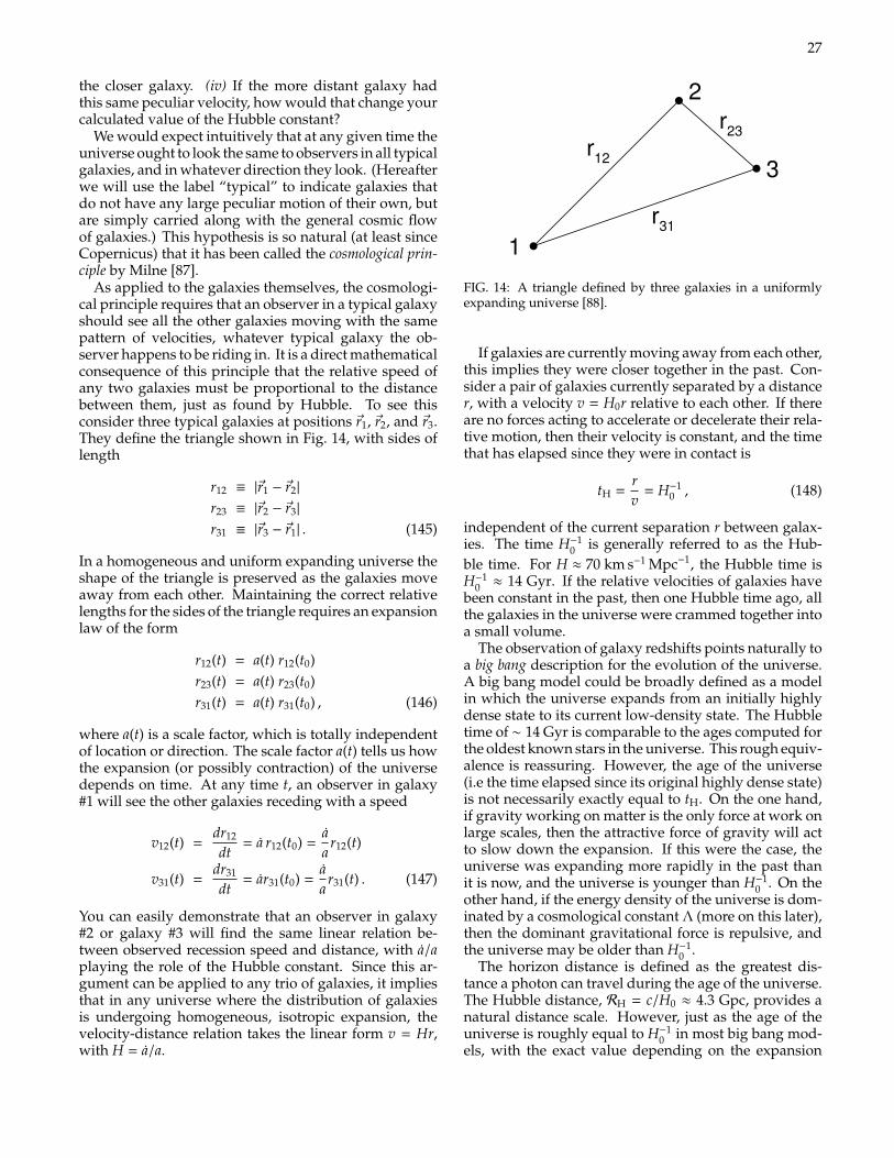
27

the closer galaxy. (iv) If the more distant galaxy hadthis same peculiar velocity, how would that change yourcalculated value of the Hubble constant?

We would expect intuitively that at any given time theuniverse ought to look the same to observers in all typicalgalaxies, and in whatever direction they look. (Hereafterwe will use the label “typical” to indicate galaxies thatdo not have any large peculiar motion of their own, butare simply carried along with the general cosmic flowof galaxies.) This hypothesis is so natural (at least sinceCopernicus) that it has been called the cosmological prin-ciple by Milne [87].

As applied to the galaxies themselves, the cosmologi-cal principle requires that an observer in a typical galaxyshould see all the other galaxies moving with the samepattern of velocities, whatever typical galaxy the ob-server happens to be riding in. It is a direct mathematicalconsequence of this principle that the relative speed ofany two galaxies must be proportional to the distancebetween them, just as found by Hubble. To see thisconsider three typical galaxies at positions ~r1, ~r2, and ~r3.They define the triangle shown in Fig. 14, with sides oflength

r12 ≡ |~r1 − ~r2|

r23 ≡ |~r2 − ~r3|

r31 ≡ |~r3 − ~r1| . (145)

In a homogeneous and uniform expanding universe theshape of the triangle is preserved as the galaxies moveaway from each other. Maintaining the correct relativelengths for the sides of the triangle requires an expansionlaw of the form

r12(t) = a(t) r12(t0)r23(t) = a(t) r23(t0)r31(t) = a(t) r31(t0) , (146)

where a(t) is a scale factor, which is totally independentof location or direction. The scale factor a(t) tells us howthe expansion (or possibly contraction) of the universedepends on time. At any time t, an observer in galaxy#1 will see the other galaxies receding with a speed

v12(t) =dr12

dt= a r12(t0) =

aa

r12(t)

v31(t) =dr31

dt= ar31(t0) =

aa

r31(t) . (147)

You can easily demonstrate that an observer in galaxy#2 or galaxy #3 will find the same linear relation be-tween observed recession speed and distance, with a/aplaying the role of the Hubble constant. Since this ar-gument can be applied to any trio of galaxies, it impliesthat in any universe where the distribution of galaxiesis undergoing homogeneous, isotropic expansion, thevelocity-distance relation takes the linear form v = Hr,with H = a/a.

18 CHAPTER 2. FUNDAMENTAL OBSERVATIONS

1

2

3 r12

r23

r31

Figure 2.6: A triangle defined by three galaxies in a uniformly expandinguniverse.

Hubble Space Telescope. The best current estimate of the Hubble constant,combining the results of di!erent research groups, is

H0 = 70 ± 7 km s!1 Mpc!1 . (2.7)

This is the value for the Hubble constant that I will use in the remainder ofthis book.

Cosmological innocents sometimes exclaim, when first encountering Hub-ble’s Law, “Surely it must be a violation of the cosmological principle tohave all those distant galaxies moving away from us ! It looks as if we areat a special location in the universe – the point away from which all othergalaxies are fleeing.” In fact, what we see here in our Galaxy is exactly whatyou would expect to see in a universe which is undergoing homogeneous andisotropic expansion. We see distant galaxies moving away from us; but ob-servers in any other galaxy would also see distant galaxies moving away fromthem.

To see on a more mathematical level what we mean by homogeneous,isotropic expansion, consider three galaxies at positions !r1, !r2, and !r3. Theydefine a triangle (Figure 2.6) with sides of length

r12 ! |!r1 " !r2| (2.8)

r23 ! |!r2 " !r3| (2.9)

r31 ! |!r3 " !r1| . (2.10)

FIG. 14: A triangle defined by three galaxies in a uniformlyexpanding universe [88].

If galaxies are currently moving away from each other,this implies they were closer together in the past. Con-sider a pair of galaxies currently separated by a distancer, with a velocity v = H0r relative to each other. If thereare no forces acting to accelerate or decelerate their rela-tive motion, then their velocity is constant, and the timethat has elapsed since they were in contact is

tH =rv

= H−10 , (148)

independent of the current separation r between galax-ies. The time H−1

0 is generally referred to as the Hub-ble time. For H ≈ 70 km s−1 Mpc−1, the Hubble time isH−1

0 ≈ 14 Gyr. If the relative velocities of galaxies havebeen constant in the past, then one Hubble time ago, allthe galaxies in the universe were crammed together intoa small volume.

The observation of galaxy redshifts points naturally toa big bang description for the evolution of the universe.A big bang model could be broadly defined as a modelin which the universe expands from an initially highlydense state to its current low-density state. The Hubbletime of ∼ 14 Gyr is comparable to the ages computed forthe oldest known stars in the universe. This rough equiv-alence is reassuring. However, the age of the universe(i.e the time elapsed since its original highly dense state)is not necessarily exactly equal to tH. On the one hand,if gravity working on matter is the only force at work onlarge scales, then the attractive force of gravity will actto slow down the expansion. If this were the case, theuniverse was expanding more rapidly in the past thanit is now, and the universe is younger than H−1

0 . On theother hand, if the energy density of the universe is dom-inated by a cosmological constant Λ (more on this later),then the dominant gravitational force is repulsive, andthe universe may be older than H−1

0 .The horizon distance is defined as the greatest dis-

tance a photon can travel during the age of the universe.The Hubble distance, RH = c/H0 ≈ 4.3 Gpc, provides anatural distance scale. However, just as the age of theuniverse is roughly equal to H−1

0 in most big bang mod-els, with the exact value depending on the expansion

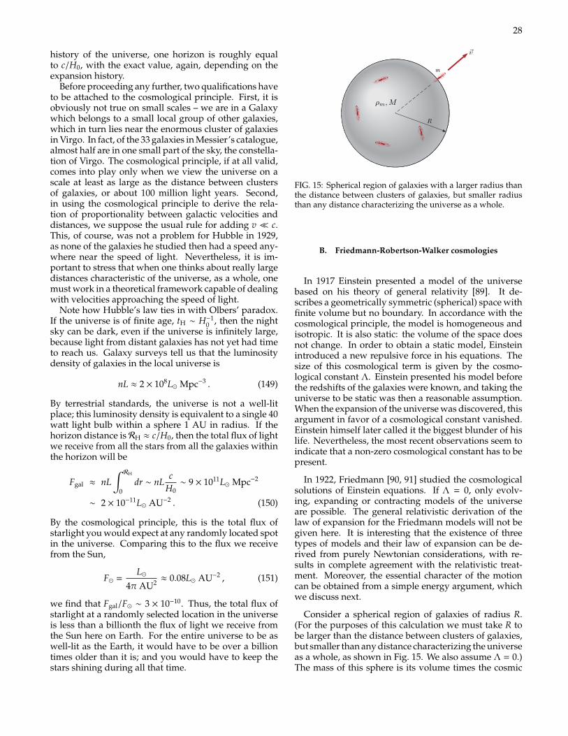
28

history of the universe, one horizon is roughly equalto c/H0, with the exact value, again, depending on theexpansion history.

Before proceeding any further, two qualifications haveto be attached to the cosmological principle. First, it isobviously not true on small scales – we are in a Galaxywhich belongs to a small local group of other galaxies,which in turn lies near the enormous cluster of galaxiesin Virgo. In fact, of the 33 galaxies in Messier’s catalogue,almost half are in one small part of the sky, the constella-tion of Virgo. The cosmological principle, if at all valid,comes into play only when we view the universe on ascale at least as large as the distance between clustersof galaxies, or about 100 million light years. Second,in using the cosmological principle to derive the rela-tion of proportionality between galactic velocities anddistances, we suppose the usual rule for adding v c.This, of course, was not a problem for Hubble in 1929,as none of the galaxies he studied then had a speed any-where near the speed of light. Nevertheless, it is im-portant to stress that when one thinks about really largedistances characteristic of the universe, as a whole, onemust work in a theoretical framework capable of dealingwith velocities approaching the speed of light.

Note how Hubble’s law ties in with Olbers’ paradox.If the universe is of finite age, tH ∼ H−1

0 , then the nightsky can be dark, even if the universe is infinitely large,because light from distant galaxies has not yet had timeto reach us. Galaxy surveys tell us that the luminositydensity of galaxies in the local universe is

nL ≈ 2 × 108L Mpc−3 . (149)

By terrestrial standards, the universe is not a well-litplace; this luminosity density is equivalent to a single 40watt light bulb within a sphere 1 AU in radius. If thehorizon distance isRH ≈ c/H0, then the total flux of lightwe receive from all the stars from all the galaxies withinthe horizon will be

Fgal ≈ nL∫RH

0dr ∼ nL

cH0∼ 9 × 1011L Mpc−2

∼ 2 × 10−11L AU−2 . (150)

By the cosmological principle, this is the total flux ofstarlight you would expect at any randomly located spotin the universe. Comparing this to the flux we receivefrom the Sun,

F =L

4π AU2 ≈ 0.08L AU−2 , (151)

we find that Fgal/F ∼ 3 × 10−10. Thus, the total flux ofstarlight at a randomly selected location in the universeis less than a billionth the flux of light we receive fromthe Sun here on Earth. For the entire universe to be aswell-lit as the Earth, it would have to be over a billiontimes older than it is; and you would have to keep thestars shining during all that time.

16.6 FREIDMANN MODELS AND THE AGE OF THE UNIVERSE

Freidmann’s work established the foundation for describing the time evolu-tion of the Universe based on general relativity. General relativity must beused in cosmological calculations because it correctly describes gravity, themost important force determining the Universe’s structure, over immense cos-mological distances. Newtonian theory can lead to errors when applied to theUniverse as a whole because it assumes that the force of gravity is always attrac-tive and is instantaneously transmitted. Although Freidmann did considermodels both with and without Einstein’s repulsive form of gravity (cosmologi-cal constant), it is easiest to see the general form of Big Bang behavior withoutintroducing repulsive gravitational forces at this point.

Freidmann found three types of time-dependent universes, which may bedescribed in terms of the universal expansion scaling factor a(t). Figure 16.17shows a(t )(the separation between galaxies) as a function of time for thethree cases labeled open universe, flat universe, and closed universe. Note thata(t) alone has a value of zero at the lower-left corner of the graph, not t, andthat the three curves start at different times in the past in order to give thesame scaling factor at the present time, denoted t0. Open universes have lessmass and energy than that needed to halt the expansion. They start with a scalefactor of zero and grow without limit, any given galaxy approaching a limiting

22 CHAPTER 16 COSMOLOGY

EXAMPLE 16.2 Critical Density of the Universe

We can estimate the critical mass density of the Universe,!c, using classical energy considerations. The result turnsout to be in agreement with the rigorous predictions ofgeneral relativity because of the simplifying assumptionthat the mass of the Universe is uniformly distributed.

Solution Figure 16.16 shows a large section of the Uni-verse with radius R with the critical density, containing atotal mass M, where M consists of the total mass of matterplus the effective mass of radiation with energy E, E/c2. Agalaxy of mass m and speed v at R will just escape to infin-ity with zero speed if the sum of its kinetic energy andgravitational potential energy is zero. Thus,

Because the galaxy of mass m obeys the Hubble law,v " HR, the preceding equation becomes

or !c "3H 2

8#GH 2 "

8#G

3!c

v2 "8#G

3R2!c

12 mv2 "

Gm43#R3!c

R

Etotal " 0 " K $ U " 12 mv2 %

GmM

R

Using H " 23 & 10%3 m/(s · lightyear), where 1 light-year " 9.46 & 1015 m and G " 6.67 & 10%11 N · m2/kg2,yields a present value of the critical density !c " 1.1 &10%26 kg/m3. As the mass of a hydrogen atom is 1.67 &10%27 kg, !c corresponds to about 7 hydrogen atoms percubic meter, an incredibly low density.

R

v

m

Figure 16.16 (Example 16.2) A galaxy escaping from alarge cluster contained within radius R. Only the masswithin R slows the mass m.

Copyright 2005 Thomson Learning, Inc. All Rights Reserved.

m, M

~v

FIG. 15: Spherical region of galaxies with a larger radius thanthe distance between clusters of galaxies, but smaller radiusthan any distance characterizing the universe as a whole.

B. Friedmann-Robertson-Walker cosmologies

In 1917 Einstein presented a model of the universebased on his theory of general relativity [89]. It de-scribes a geometrically symmetric (spherical) space withfinite volume but no boundary. In accordance with thecosmological principle, the model is homogeneous andisotropic. It is also static: the volume of the space doesnot change. In order to obtain a static model, Einsteinintroduced a new repulsive force in his equations. Thesize of this cosmological term is given by the cosmo-logical constant Λ. Einstein presented his model beforethe redshifts of the galaxies were known, and taking theuniverse to be static was then a reasonable assumption.When the expansion of the universe was discovered, thisargument in favor of a cosmological constant vanished.Einstein himself later called it the biggest blunder of hislife. Nevertheless, the most recent observations seem toindicate that a non-zero cosmological constant has to bepresent.

In 1922, Friedmann [90, 91] studied the cosmologicalsolutions of Einstein equations. If Λ = 0, only evolv-ing, expanding or contracting models of the universeare possible. The general relativistic derivation of thelaw of expansion for the Friedmann models will not begiven here. It is interesting that the existence of threetypes of models and their law of expansion can be de-rived from purely Newtonian considerations, with re-sults in complete agreement with the relativistic treat-ment. Moreover, the essential character of the motioncan be obtained from a simple energy argument, whichwe discuss next.

Consider a spherical region of galaxies of radius R.(For the purposes of this calculation we must take R tobe larger than the distance between clusters of galaxies,but smaller than any distance characterizing the universeas a whole, as shown in Fig. 15. We also assume Λ = 0.)The mass of this sphere is its volume times the cosmic

29

mass density,

M =4πR3

3ρm . (152)

We can now consider the motion of a galaxy of mass mat the edge of the spherical region. According to Hub-ble’s law, the velocity of the galaxy is v = HR, and itscorresponding kinetic energy

K =12

mv2 =12

mH2R2 . (153)

In a spherical distribution of matter, the gravitationalforce on a given spherical shell depends only on themass inside the shell. The potential energy at the edgeof the sphere is

U = −GMm

R= −

4πmR2ρmG3

. (154)

Hence, the total energy is

E = K + U =12

mH2R2− Gm

4π3

R2ρm . (155)

which has to remain constant as the universe expands.Likewise,

2EmR2 = H2

−8π3

Gρm . (156)

Since we assume that the universe is homogeneous, Hand ρm cannot be functions of R. Thus, the left-hand-side of (156) cannot depend on the chosen distance R tothe coordinate center. However, the value of 2E/(mR2)is time-dependent, because the distance between us andthe galaxy will change as the universe expands. Sincethe mass m of our test galaxy is arbitrary, we can chooseit such that |2E/(mc2)| = 1 holds at an arbitrary momentas long as E , 0. For different times, the left-hand-sidescales as R−2 and thus we can rewrite (156) as( a

a

)2=

8π3

Gρm −kc2

a2R20

. (157)

Note that because E is constant, k is constant too. Ac-tually, k = 0,±1 is generally known as the curvatureconstant. Throughout the subscripted “0”s indicate thatquantities (which in general evolve with time) are to beevaluated at present epoch. Finally, we account for theequivalence of mass and energy by including not onlythe mass but also the energy density, ρ = ρmc2 + · · · andso (157) becomes

H2≡

( aa

)2=

8π3

Gρ

c2 −kc2

a2R20

. (158)

which is Friedmann equation (without cosmological con-stant) in the Newtonian limit. (158) agrees exactly with

the equation derived from general relativity [63]. Fork = 0, the value of H fixes the so-called critical density as

ρ(k = 0) ≡ ρc =3H2c2

8πG. (159)

Since we know the current value of the Hubble parame-ter to within 10%, we can compute the current value ofthe critical density to within 20%. We usually hide thisuncertainty by introducing h,

H0 = 100 h km s−1 Mpc−1 , (160)

such that

ρc,0 = 2.77 × 1011h2M/Mpc3

= 1.88 × 10−29h2g/cm3

= 1.05 × 10−5h2 GeV/cm3 . (161)

Note that since h ≈ 0.70+0.05−0.03 a flat universe requires an

energy density of ∼ 10 protons per cubic meter.The expansion of the universe can be compared to the

motion of a mass launched vertically from the surfaceof a celestial body. The form of the orbit depends onthe initial energy. In order to compute the complete or-bit, the mass of the main body and the initial velocityhave to be known. In cosmology, the correspondingparameters are the mean density and the Hubble con-stant. On the one hand, if the density exceeds the critialdensity, the expansion of any spherical region will turnto a contraction and it will collapse to a point. Thiscorresponds to the closed Friedmann model. On theother hand, if ρm < ρc, the ever-expanding hyperbolicmodel is obtained. These three models of the universeare called the standard models. They are the simplestrelativistic cosmological models for Λ = 0. Models withΛ , 0 are mathematically more complicated, but showthe same behaviour. The simple Newtonian treatmentof the expansion problem is possible because Newtonianmechanics is approximately valid in small regions of theuniverse. However, although the resulting equationsare formally similar, the interpretation of the quantitiesinvolved is not the same as in the relativistic context.The global geometry of Friedmann models can only beunderstood within the general theory of relativity [63].

Next, we define the abundance Ωi of the different play-ers in cosmology as their energy density relative to ρc.For example, the dimensionless mass density parameteris found to be

Ωm =ρmc2

ρc=

8πG3H2 ρm . (162)

For simplicity, for the moment we will keep consideringscenarios with Λ = 0, but we advance the reader that

ΩΛ =Λc2

3H2 . (163)

Now, what about our universe? On a large scalewhat is the overall curvature of the universe? Does it

30

have positive curvature, negative curvature, or is it flat?By solving Einstein equations, Robertson [92, 93] andWalker [94], showed that the three hypersurfaces of con-stant curvature (the hyper-sphere, the hyper-plane, andthe hyper-pseudosphere) are indeed possible geometriesfor a homegeneous and isotropic universe undergoingexpansion. The metric they derived, independently ofeach other, is called the Friedmann-Robertson-Walker(FRW) metric. The line element is most generally writ-ten in the form

ds2 = c2dt2− a2(t)

[d%2

1 − k%2/R2 + %2dΩ2

], (164)

where dΩ2 = dθ2+sin2 θdφ2. It is easily seen that the spa-tial component of the FRW metric consists of the spatialmetric for a uniformly curved space of radius R, scaledby the square of the scale factor a(t). If the universe hada positive curvature k = 1, then the universe would beclosed, or finite in volume. This would not mean that thestars and galaxies extended out to a certain boundary, be-yond which there is empty space. There is no boundaryor edge in such a universe. If a particle were to move in astraight line in a particular direction, it would eventuallyreturn to the starting point – perhaps eons of time later.On the other hand, if the curvature of the space was zerok = 0 or negative k = −1, the universe would be open. Itcould just go on forever.

Using the substitution

% = Sk(r) =

R sin(r/R) for k = +1r for k = 0R sinh(r/R) for k = −1

; (165)

the FRW line element can be rewritten as

ds2 = c2dt2− a2(t)

[dr2 + S2

k(r) dΩ2]

; (166)

see Appendix E for details.The time variable t in the FRW metric is the cosmolog-

ical proper time, called the cosmic time for short, and isthe time measured by an observer who sees the universeexpanding uniformly around him. The spatial variables(%, θ, φ) or (r, θ, φ) are called the comoving coordinatesof a point in space. If the expansion of the universeis perfectly homogeneous and isotropic, the comovingcoordinates of any point remain constant with time.

To describe the time evolution of the scale factor a(t) weneed an additional equation describing how the energycontent of the universe ρ is affected by expansion. Thefirst law of thermodynamics,

dU = TdS − PdV, (167)

with dQ = 0 (no heat exchange to the outside, since nooutside exists) becomes

dU = −PdV ⇒dUdt

+ PdVdt

= 0 . (168)

There is a caveat to the statement that the expansion of ahomogeneous universe is adiabatic: when particles anni-hilate, such as electrons and positrons, this adds heat andmakes the expansion temporarily non-adiabatic. Thismatters at some specific epochs in the very early uni-verse.

For a sphere of comoving radius R0,

V =43πR3

0 a3(t) , (169)

and so

V = 4πR30 a2 a = 3

aa

V . (170)

Since U = ρV,

U = ρV + ρV = V(ρ + 3

aaρ). (171)

Substituting (170) and (171) into (168) we have

V(ρ + 3

aaρ + 3

aa

P)

= 0 (172)

and thus

ρ = −3(ρ + P

) aa. (173)

This fluid equation describes the evolution of energy den-sity in an expanding universe. It tells us that the ex-pansion decreases the energy density both by dilutionand by the work required to expand a gas with pressureP ≥ 0.

To solve this equation, we need an additional equationof state relating P and ρ. Suppose we write this in theform

P = wρ . (174)

In principle, w could change with time, but we will as-sume that any time derivatives of w are negligible com-pared to time derivatives of ρ. This is reasonable if theequation of state is determined by “microphysics” thatis not directly tied to the expansion of the universe. Thefluid equation then implies

ρ

ρ= −3(1 + w)

aa, (175)

with solution

ρ

ρ0=

( aa0

)−3(1+w). (176)

The pressure in a gas is determined by the thermal mo-tion of its constituents. For non-relativistic matter (a.k.a.cosmological dust),

w =Pρ∼

mv2

mc2 ∼vc2 1 , (177)

31

where v is the thermal velocity of particles with massm. To a near-perfect approximation w = 0, implyingρm ∝ a−3. Light, or more generally any highly relativisticparticle, has an associated pressure (radiation pressure).Pressure is defined as the momentum transfer onto aperfectly reflecting wall per unit time and per unit area.Consider an isotropic distribution of photons (or anotherkind of particle) moving with the speed of light. The mo-mentum of a photon is given in terms of its energy asp = E/c = hν/c. Consider now an area element dA ofthe wall; the momentum transferred to it per unit timeis given by the momentum transfer per photon, timesthe number of photons hitting the area dA per unit time.We will assume for the moment that all photons havethe same frequency. If θ denotes the direction of a pho-ton relative to the normal of the wall, the momentumcomponent perpendicular to the wall before scatteringis p⊥ = p cosθ, and after scattering p⊥ = −p cosθ; thetwo other momentum components are unchanged bythe reflection. Thus, the momentum transfer per pho-ton scattering is ∆p = 2p cosθ. The number of photonsscattering per unit time within the area dA is given bythe number density of photons, n times the area elementdA, times the thickness of the layer from which photonsarrive at the wall per unit time. The latter is given byc cosθ, since only the perpendicular velocity componentbrings them closer to the wall. Putting these terms to-gether, we find for the momentum transfer to the wallper unit time per unit area the expression

P(θ) = 2hν n cos2 θ . (178)

Averaging this expression over a half-sphere (only pho-tons moving towards the wall can hit it) then yields

P =13

hνn =13ρ . (179)

Then for radition, w = 1/3, implying ρrad ∝ a−4. This be-havior also follows from a simple argument: the numberdensity of photons falls as n ∝ a−3, and the energy perphoton falls as hν ∝ a−1 because of cosmological redshift(more on this below).

Next, we obtain an expression for the acceleration ofthe universe. If we multiply our standard version of theFriedmann equation by a2, we get

a2 =8πG3c2 ρa2

−kc2

R20

. (180)

Take the time derivative of (180)

2aa =8πG3c2

(ρa2 + 2ρaa

). (181)

divide by 2aa

aa

=4πG3c2

(ρ

aa

+ 2ρ), (182)

and substitutte from the fluid equation

ρaa

= −3(ρ + P) (183)

to obtain the acceleration equation

aa

= −4πG3c2 (ρ + 3P) . (184)

We see that if ρ and P are positive, the expansion of theuniverse decelerates. Higher P produces stronger decel-eration for given ρ, e.g., a radiation-dominated universedecelerates faster than a matter-dominated universe.

In the remainder of this section, we consider a flat uni-verse, i.e., k = 0. It is easily seen that for non-relativisticmatter, the solution to Friedmann equation (158) is givenby

a(t) =( t

t0

)2/3and ρ(t) =

ρ0

a3 =ρ0t2

0

t2 , (185)

with

t0 =23

1H0

, (186)

where we have used (159). Following the same steps for abizarre universe, which is dominated today by radiationpressure, yields the solution

a(t) =( t

t0

)1/2and ρ(t) =

ρ0

a4 =ρ0t2

0

t2 . (187)

From this simple exercise we can picture the the timeevolution of the universe as follows. In the earlyuniverse all matter is relativistic and radiation pressuredominates: a(t) ∝ t1/2, ρrad ∝ t−2, and ρm ∝ a−3

∝ t−3/2.The density of radiation then falls more quickly thanthat of dust. On the other hand, when dust dominates:a(t) ∝ t2/3, ρm ∝ t−2, and ρrad ∝ a−4

∝ t8/3, hence dustdomination increases.

EXERCISE 6.4 Using the Hubble flow v = H0r showthat the expansion of the universe changes the particlenumber density according to n = −3H0n.

In closing, we discuss how to measure distances in theFRW spacetime. Consider a galaxy which is far awayfrom us, sufficiently far away that we may ignore thesmall scale perturbations of spacetime and adopt theFRW line element. In an expanding universe, the dis-tance between two objects is increasing with time. Thus,if we want to assign a spatial distance between two ob-jects, we must specify the time t at which the distanceis the correct one. Suppose that you are at the origin,and that the galaxy which you are observing is at a co-moving coordinate position (r, θ, φ). We define a properdistance, as the distance between two events A and B ina reference frame for which they occur simultaneously

32

(tA = tB). In other words, the proper distance dp(t) be-tween two points in spacetime is equal to the length ofthe spatial geodesic between them when the scale factoris fixed at the value a(t). The proper distance betweenthe observer and galaxy can be found using the FRWmetric at a fixed time t,

ds2 = a2(t)[dr2 + S2

k(r) dΩ2]. (188)

Along the spatial geodesic between the observer andgalaxy, the angle (θ, φ) is constant, and thus

ds = a(t) dr . (189)

Likewise, using spatial variables (%, θ, φ) we have

ds = a(t)[1 − k(%/R)2]−1/2 dr (190)

The proper distance dp is found by integrating over theradial comoving coordinate r

dp = a(t)∫ r

0dr = a(t) r , (191)

or using (165)

dp = a(t)

k−1/2 sin−1(

√k%/R) for k = +1

% for k = 0|k|−1/2 sinh−1(

√|k|%/R) for k = −1

. (192)

In a flat universe, the proper distance to an objectis just its coordinate distance, dp(t) = a(t)%. Becausesin−1(x) > x and sinh−1(x) < x, in a closed universe(k > 0) the proper distance to an object is greater than itscoordinate distance, while in an open universe (k < 0)the proper distance to an object is less than its coordinatedistance.

EXERCISE 6.5 A civilization that wants to conquerthe universe, which is homogeneous and isotropic, andhence is described by the FRW metric, is getting readyto send out soldiers in all directions to invade all theuniverse out to a proper distance dp. Every soldierleaves the galaxy where the civilization was born, andtravels through the universe with its spaceship along ageodesic, out to a distance dp from the original galaxy.At the end of the invasion, which occurs at a fixedtime t, all the soldiers stand on a spherical surface at aproper distance dp from their original galaxy. The totalvolume that has been invaded is the volume inside thisspherical surface. What is the total volume invaded?Answer this question for the following three cases:(i) A flat metric (k = 0). (ii) A closed metric (k = +1)with radius of curvature R at the cosmic time t whenthe invaded volume and the proper distance dp aremeasured. (iii) An open metric (k = −1) with radiusof curvature R at the cosmic time t when the invadedvolume and the proper distance dp are measured.

EXERCISE 6.6 Consider a positively curved universe(k = 1), in which the sole contribution to the energydensity comes from non-relativistic matter. In this casethe energy density has the dependence ρm = ρm,0/a3.(i) Write down Friedmann equation for this universe andshow that the parametric solution,

a(θ) =4πGρm,0R2

0

3c4 (1 − cosθ) ,

t(θ) =4πGρm,0R3

0

3c5 (θ − sinθ) , (193)

satisfies the Friedmann equation. Here θ is a dimen-sionless parameter that runs from 0 to 2π, and R0 isthe present radius of curvature if we have normalizedthe scale factor at present to a(t0) = 1. (ii) What is amax,the maximum possible scale factor for this universe?(iii) What is the maximum value that the physical radiusof curvature (aR0) reaches? (iv) What is the age ofthe universe when this maximum radius is reached?(v) What is tcrunch, the time at which the universeundergoes a big crunch (that is a recollapse to a = 0)?[Hint: Recall that a = da/dt = da/dθ dθ/dt.]

EXERCISE 6.7 Consider a positively curved universe(k = −1), in which the sole contribution to the energydensity comes from non-relativistic matter, and so the en-ergy density has the dependence ρm = ρm,0/a3. (ii) Writedown Friedmann equation for this universe and showthat the parametric solution,

a(θ) =4πGρm,0R2

0

3c4 (coshθ − 1) ,

t(θ) =4πGρm,0R3

0

3c5 (sinhθ − θ) , (194)

satisfies the Friedmann equation. (ii) Compare the timedependence of the scale factor for open, closed andcritical matter-dominated cosmological models in alog-log plot.

C. Age and size of the Universe

In special (and general) relativity the propagation oflight is along a null geodesic (ds = 0). If we place theobserver at the origin (% = 0), and we choose a radialnull geodesic (dθ = dφ = 0), we have

cdta(t)

= ±d%

[1 − k(%/R)2]1/2, (195)

where + is for the emitted light ray and the − is for a re-ceived one. Imagine now that one crest of the light wavewas emitted at time tem at distance %em, and received atthe origin %0 = 0 at t0, and that the next wave crest was

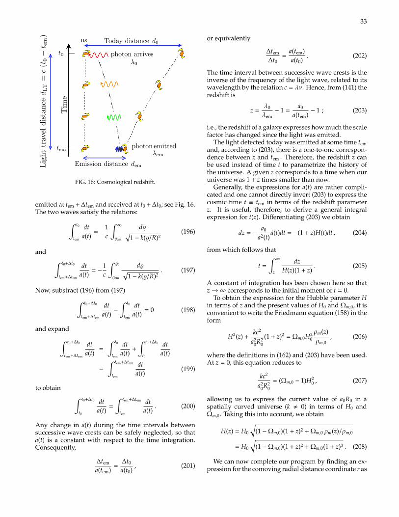
33

Distances in Cosmology

photon emitted

Emission distance, dem

Today distance, d0

photon arrives

em

0

us

tem

t0

Tim

e

Lig

ht

trav

eldis

tance

dLT

=c

(t0

t em

)

FIG. 16: Cosmological redshift.

emitted at tem + ∆tem and received at t0 + ∆t0; see Fig. 16.The two waves satisfy the relations:∫ t0

tem

dta(t)

= −1c

∫ %0

%em

d%√1 − k(%/R)2

(196)

and ∫ t0+∆t0

tem+∆tem

dta(t)

= −1c

∫ %0

%em

d%√1 − k(%/R)2

. (197)

Now, substract (196) from (197)∫ t0+∆t0

tem+∆tem

dta(t)−

∫ t0

tem

dta(t)

= 0 (198)

and expand∫ t0+∆t0

tem+∆tem

dta(t)

=

∫ t0

tem

dta(t)

+

∫ t0+∆t0

t0

dta(t)

−

∫ tem+∆tem

tem

dta(t)

(199)

to obtain ∫ t0+∆t0

t0

dta(t)

=

∫ tem+∆tem

tem

dta(t)

. (200)

Any change in a(t) during the time intervals betweensuccessive wave crests can be safely neglected, so thata(t) is a constant with respect to the time integration.Consequently,

∆tem

a(tem)=

∆t0

a(t0), (201)

or equivalently

∆tem

∆t0=

a(tem)a(t0)

. (202)

The time interval between successive wave crests is theinverse of the frequency of the light wave, related to itswavelength by the relation c = λν. Hence, from (141) theredshift is

z =λ0

λem− 1 =

a0

a(tem)− 1 ; (203)

i.e., the redshift of a galaxy expresses how much the scalefactor has changed since the light was emitted.

The light detected today was emitted at some time temand, according to (203), there is a one-to-one correspon-dence between z and tem. Therefore, the redshift z canbe used instead of time t to parametrize the history ofthe universe. A given z corresponds to a time when ouruniverse was 1 + z times smaller than now.

Generally, the expressions for a(t) are rather compli-cated and one cannot directly invert (203) to express thecosmic time t ≡ tem in terms of the redshift parameterz. It is useful, therefore, to derive a general integralexpression for t(z). Differentiating (203) we obtain

dz = −a0

a2(t)a(t)dt = −(1 + z)H(t)dt , (204)

from which follows that

t =

∫∞

z

dzH(z)(1 + z)

. (205)

A constant of integration has been chosen here so thatz→∞ corresponds to the initial moment of t = 0.

To obtain the expression for the Hubble parameter Hin terms of z and the present values of H0 and Ωm,0, it isconvenient to write the Friedmann equation (158) in theform

H2(z) +kc2

a20R2

0

(1 + z)2 = Ωm,0H20ρm(z)ρm,0

, (206)

where the definitions in (162) and (203) have been used.At z = 0, this equation reduces to

kc2

a20R2

0

= (Ωm,0 − 1)H20 , (207)

allowing us to express the current value of a0R0 in aspatially curved universe (k , 0) in terms of H0 andΩm,0. Taking this into account, we obtain

H(z) = H0

√(1 −Ωm,0)(1 + z)2 + Ωm,0 ρm(z)/ρm,0

= H0

√(1 −Ωm,0)(1 + z)2 + Ωm,0(1 + z)3 . (208)

We can now complete our program by finding an ex-pression for the comoving radial distance coordinate r as

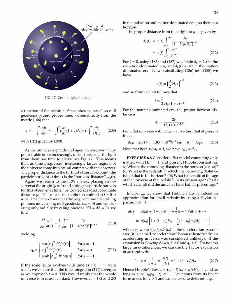
34

The Horizon

Radius ofobservable universe

FIG. 17: Cosmological horizon.

a function of the reshift z. Since photons travel on nullgeodesics of zero proper time, we see directly from themetric (166) that

r = −

∫cdta(t)

= −

∫c

dtdz

(1 + z)dz = c∫

dzH(z)

, (209)

with H(z) given by (208).

As the universe expands and ages, an observer at anypoint is able to see increasingly distant objects as the lightfrom them has time to arrive, see Fig. 17. This meansthat, as time progresses, increasingly larger regions ofthe universe come into causal contact with the observer.The proper distance to the furthest observable point (theparticle horizon) at time t is the “horizon distance”, dh(t).

Again we return to the FRW metric, placing an ob-server at the origin (% = 0) and letting the particle horizonfor this observer at time t be located at radial coordinatedistance %h. This means that a photon emitted at t = 0 at%h will reach the observer at the origin at time t. Recallingphotons move along null geodesics (ds = 0) and consid-ering only radially traveling photons (dθ = dφ = 0), wefind ∫ t

0

dt′

a(t′)=

1c

∫ %h

0

d%[1 − k(%/R)2]1/2

, (210)

yielding

%h =

sin

[c∫ t

0 dt′/a(t′)]

for k = +1

c∫ t

0 dt′/a(t′) for k = 0

sinh[c∫ t

0 dt′/a(t′)]

for k = −1

. (211)

If the scale factor evolves with time as a(t) = tα, withα > 1, we can see that the time integral in (211) divergesas we approach t = 0. This would imply that the wholeuniverse is in causal contact. However, α = 1/2 and 2/3

in the radiation and matter-dominated eras, so there is ahorizon.

The proper distance from the origin to %h is given by

dh(t) = a(t)∫ %h

0

d%[1 − k(%/R)2]1/2

= a(t)∫ t

0

cdt′

a(t′). (212)

For k = 0, using (185) and (187) we obtain dh = 2ct in theradiation-dominated era, and dh(t) = 3ct in the matter-dominated era. Now, substituting (186) into (185) wehave

a(t) =(3

2H0 t

)2/3

(213)

and so from (203) it follows that

t =23

1H0 (1 + z)3/2

. (214)

For the matter-dominated era, the proper horizon dis-tance is

dh =2c

H0 (1 + z)3/2. (215)

For a flat universe with Ωm,0 = 1, we find that at presenttime,

dh,0 = 2c/H0 = 1.85 × 1028h−1 cm = 6 h−1 Gpc . (216)

Note that because a0 = 1, we have %h,0 = dh,0.

EXERCISE 6.8 Consider a flat model containing onlymatter, with Ωm,0 = 1, and present Hubble constant H0.(i) What is the comoving distance to the horizon (z = ∞)?(ii) What is the redshift at which the comoving distanceis half that to the horizon? (iii) What is the ratio of the ageof the universe at that redshift, to its present age? (iv) Atwhich redshift did the universe have half its present age?

In closing, we show that Hubble’s law is indeed anapproximation for small redshift by using a Taylor ex-pansion of a(t),

a(t) = a(t0) + (t − t0)a(t0) +12

(t − t0)2a(t0) + · · ·

= a(t0)[1 + (t − t0)H0 −

12

(t − t0)2q0H20 + · · ·

],

where q0 ≡ −a(t0)a(t0)/a2(t0) is the deceleration param-eter (it is named “deceleration” because historically, anaccelerating universe was considered unlikely). If theexpansion is slowing down, a < 0 and q0 > 0. For not toolarge time-differences, we can use the Taylor expansionof a(t) and write

1 − z ≈1

1 + z=

a(t)a(t0)

≈ 1 + (t − t0)H0 . (217)

Hence Hubble’s law, z = (t0 − t)H0 = d/cH0, is valid aslong as z H0(t0 − t) 1. Deviations from its linearform arises for z & 1 and can be used to determine q0.

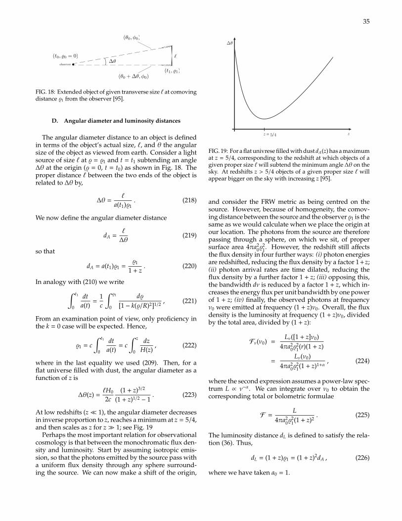
352.5 Kinematic tests 61

observer

l

χem

ϕ0 tem

∆θ

θ0 + ∆θ

χ = 0t = t0

ϕ0 = const

θ0 = const

Fig. 2.11.

tem propagate along radial geodesics and arrive today with an apparent angularseparation !θ . The proper size of the object, l, is equal to the interval between theemission events at the endpoints:

l =!

−!s2 = a(tem) #(χem) !θ, (2.68)

as obtained from metric (2.2). The angle subtended by the object is then

!θ = la(tem) #(χem)

= la(η0 − χem) #(χem)

, (2.69)

where we have used the fact that the physical time tem corresponds to the conformaltime ηem = η0 − χem . If the object is close to us, that is, χem ≪ η0, then

a(η0 − χem) ≈ a(η0) , #(χem) ≈ χem,

and

!θ ≈ la(η0) χem

= lD

.

We see that in this case !θ is inversely proportional to the distance, as expected.However, if the object is located far away, namely, close to the particle horizon,then η0 − χem ≪ η0, and

a(η0 − χem) ≪ a(η0) , #(χem) → #"χp

#= const.

The angular size of the object,

!θ ∝ la(η0 − χem)

,

`

(0,0)

(0 + ,0)

(t1, %1)

(t0, %0 = 0)

FIG. 18: Extended object of given transverse size ` at comovingdistance %1 from the observer [95].

D. Angular diameter and luminosity distances

The angular diameter distance to an object is definedin terms of the object’s actual size, `, and θ the angularsize of the object as viewed from earth. Consider a lightsource of size ` at % = %1 and t = t1 subtending an angle∆θ at the origin (% = 0, t = t0) as shown in Fig. 18. Theproper distance ` between the two ends of the object isrelated to ∆θ by,

∆θ =`

a(t1)%1. (218)

We now define the angular diameter distance

dA =`

∆θ(219)

so that

dA = a(t1)%1 =%1

1 + z. (220)

In analogy with (210) we write∫ t1

0

dta(t)

=1c

∫ %1

0

d%[1 − k(%/R)2]1/2

, (221)

From an examination point of view, only proficiency inthe k = 0 case will be expected. Hence,

%1 = c∫ t1

0

dta(t)

= c∫ z

0

dzH(z)

, (222)

where in the last equality we used (209). Then, for aflat universe filled with dust, the angular diameter as afunction of z is

∆θ(z) =`H0

2c(1 + z)3/2

(1 + z)1/2 − 1. (223)

At low redshifts (z 1), the angular diameter decreasesin inverse proportion to z, reaches a minimum at z = 5/4,and then scales as z for z 1; see Fig. 19

Perhaps the most important relation for observationalcosmology is that between the monochromatic flux den-sity and luminosity. Start by assuming isotropic emis-sion, so that the photons emitted by the source pass witha uniform flux density through any sphere surround-ing the source. We can now make a shift of the origin,

2.5 Kinematic tests 63

z

∆θ

z = 5/4

Fig. 2.12.

directions in the sky differs; this temperature difference depends on the angularseparation. The power spectrum is observed to have a series of peaks as the angularseparation is varied from large to small scales. The “first acoustic peak” is roughlydetermined by the sound horizon at recombination, the maximum distance that asound wave in the baryon–radiation fluid can have propagated by recombination.This sound horizon serves as a standard ruler of length ls ∼ H−1(zr ). Recombin-ation occurs at redshift zr ≃ 1100. Since !0zr ≫ 1, we can set χem(zr ) = χp in(2.70) and in a dust-dominated universe, where #

!χp

"= 2(a0 H0!0)−1 (see (2.9)),

we obtain

$θr ≃ zr H0!0

2H (zr )≃ 1

2z−1/2

r !1/20 ≃ 0.87!

1/20 . (2.73)

We have substituted here H0/H (zr ) ≃!!0z3

r

"−1/2, as follows from (2.61). Note thatin Euclidean space, the corresponding angular size would be $θr ≃ tr/t0 ≈ z−3/2

r ,or about 1000 times smaller.

The remarkable aspect of this result is that the angular diameter depends directlyonly on !0, which determines the spatial curvature, and is not very sensitive toother parameters. As we will see in Chapter 9, this is true not only for a dust-dominated universe, as considered here, but for a very wide range of cosmologicalmodels, containing multiple matter components. Hence, measuring the angularscale of the first acoustic peak has emerged as the leading and most direct methodfor determining the spatial curvature. Our best evidence that the universe is spatiallyflat (!0 = 1), as predicted by inflation, comes from this test.

FIG. 19: For a flat univrese filled with dust dA(z) has a maximumat z = 5/4, corresponding to the redshift at which objects of agiven proper size `will subtend the minimum angle ∆θ on thesky. At redshifts z > 5/4 objects of a given proper size ` willappear bigger on the sky with increasing z [95].

and consider the FRW metric as being centred on thesource. However, because of homogeneity, the comov-ing distance between the source and the observer %1 is thesame as we would calculate when we place the origin atour location. The photons from the source are thereforepassing through a sphere, on which we sit, of propersurface area 4πa2

0%21. However, the redshift still affects

the flux density in four further ways: (i) photon energiesare redshifted, reducing the flux density by a factor 1+z;(ii) photon arrival rates are time dilated, reducing theflux density by a further factor 1 + z; (iii) opposing this,the bandwidth dν is reduced by a factor 1 + z, which in-creases the energy flux per unit bandwidth by one powerof 1 + z; (iv) finally, the observed photons at frequencyν0 were emitted at frequency (1 + z)ν0. Overall, the fluxdensity is the luminosity at frequency (1 + z)ν0, dividedby the total area, divided by (1 + z):

Fν(ν0) =Lν([1 + z]ν0)

4πa20%

21(r)(1 + z)

=Lν(ν0)

4πa20%

21(1 + z)1+α

, (224)

where the second expression assumes a power-law spec-trum L ∝ ν−α. We can integrate over ν0 to obtain thecorresponding total or bolometric formulae

F =L

4πa20%

21(1 + z)2

. (225)

The luminosity distance dL is defined to satisfy the rela-tion (36). Thus,

dL = (1 + z)%1 = (1 + z)2dA , (226)

where we have taken a0 = 1.

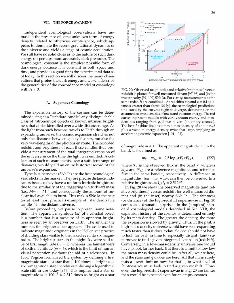
36

VII. THE FORCE AWAKENS

Independent cosmological observations have un-masked the presence of some unknown form of energydensity, related to otherwise empty space, which ap-pears to dominate the recent gravitational dynamics ofthe universe and yields a stage of cosmic acceleration.We still have no solid clues as to the nature of such darkenergy (or perhaps more accurately dark pressure). Thecosmological constant is the simplest possible form ofdark energy because it is constant in both space andtime, and provides a good fit to the experimental data asof today. In this section we will discuss the many obser-vations that probes the dark energy and we will describethe generalities of the concordance model of cosmologywith Λ , 0.

A. Supernova Cosmology

The expansion history of the cosmos can be deter-mined using as a “standard candle” any distinguishableclass of astronomical objects of known intrinsic bright-ness that can be identified over a wide distance range. Asthe light from such beacons travels to Earth through anexpanding universe, the cosmic expansion stretches notonly the distances between galaxy clusters, but also thevery wavelengths of the photons en route. The recordedredshift and brightness of each these candles thus pro-vide a measurement of the total integrated exansion ofthe universe since the time the light was emitted. A col-lection of such measurements, over a sufficient range ofdistances, would yield an entire historical record of theuniverse’s expansion.

Type Ia supernovae (SNe Ia) are the best cosmologicalyard sticks in the market. They are precise distance indi-cators because they have a uniform intrinsic brightnessdue to the similarity of the triggering white dwarf mass(i.e., MCh = M) and consequently the amount of nu-clear fuel available to burn. This makes SNe Ia the best(or at least most practical) example of “standardizablecandles” in the distant universe.

Before proceeding, we pause to present some nota-tion. The apparent magnitude (m) of a celestial objectis a number that is a measure of its apparent bright-ness as seen by an observer on Earth. The smaller thenumber, the brighter a star appears. The scale used toindicate magnitude originates in the Hellenistic practiceof dividing stars visible to the naked eye into six magni-tudes. The brightest stars in the night sky were said tobe of first magnitude (m = 1), whereas the faintest wereof sixth magnitude (m = 6), which is the limit of humanvisual perception (without the aid of a telescope). In1856, Pogson formalized the system by defining a firstmagnitude star as a star that is 100 times as bright as asixth-magnitude star, thereby establishing a logarithmicscale still in use today [96]. This implies that a star ofmagnitude m is 1001/5

' 2.512 times as bright as a star

lowed up. This approach also made it possible to use theHubble Space Telescope for follow-up light-curve observa-tions, because we could specify in advance the one-square-degree patch of sky in which our wide-field imager wouldfind its catch of supernovae. Such specificity is a require-ment for advance scheduling of the HST. By now, theBerkeley team, had grown to include some dozen collabo-rators around the world, and was called Supernova Cos-mology Project (SCP).

A community effortMeanwhile, the whole supernova community was makingprogress with the understanding of relatively nearby su-pernovae. Mario Hamuy and coworkers at Cerro Tololotook a major step forward by finding and studying manynearby (low-redshift) type Ia supernovae.7 The resultingbeautiful data set of 38 supernova light curves (someshown in figure 1) made it possible to check and improveon the results of Branch and Phillips, showing that typeIa peak brightness could be standardized.6,7

The new supernovae-on-demand techniques that per-mitted systematic study of distant supernovae and the im-proved understanding of brightness variations amongnearby type Ia’s spurred the community to redouble its ef-forts. A second collaboration, called the High-Z SupernovaSearch and led by Brian Schmidt of Australia’s MountStromlo Observatory, was formed at the end of 1994. Theteam includes many veteran supernova experts. The tworival teams raced each other over the next few years—oc-casionally covering for each other with observations whenone of us had bad weather—as we all worked feverishly tofind and study the guaranteed on-demand batches of supernovae.

At the beginning of 1997, the SCP team presented theresults for our first seven high-redshift supernovae.8 Thesefirst results demonstrated the cosmological analysis tech-niques from beginning to end. They were suggestive of anexpansion slowing down at about the rate expected for thesimplest inflationary Big Bang models, but with error barsstill too large to permit definite conclusions.

By the end of the year, the error bars began to tighten,as both groups now submitted papers with a few more su-pernovae, showing evidence for much less than the ex-pected slowing of the cosmic expansion.9–11 This was be-ginning to be a problem for the simplest inflationarymodels with a universe dominated by its mass content.

Finally, at the beginning of 1998, the two groups pre-sented the results shown in figure 3.12,13

What’s wrong with faint supernovae? The faintness—or distance—of the high-redshift super-novae in figure 3 was a dramatic surprise. In the simplest

56 April 2003 Physics Today http://www.physicstoday.org

26

24

22

20

18

16

140.01 0.02 0.04 0.1

0.2 0.4 0.6 1

OB

SER

VE

D M

AG

NIT

UD

E

22

21

200.2 0.4 0.6 1.0

Acceleratinguniverse

Deceleratinguniverse

with vacuum

energy

without vacuum energy

Mas

s de

nsit

y

0

rc

Empt

y

REDSHIFT z

0.8 0.7 0.6 0.5LINEAR SCALE OF THE UNIVERSE RELATIVE TO TODAY

Supernova CosmologyProject

High-Z SupernovaSearch

Hamuy et al.

0.0001

0.001

0.01

0.1

1

RE

LA

TIV

E B

RIG

HT

NE

SS

Exploding White Dwarfs

Aplausible, though unconfirmed, scenario would explainhow all type Ia supernovae come to be so much alike,

given the varied range of stars they start from. A lightweightstar like the Sun uses up its nuclear fuel in 5 or 10 billionyears. It then shrinks to an Earth-sized ember, a white dwarf,with its mass (mostly carbon and oxygen) supported againstfurther collapse by electron degeneracy pressure. Then itbegins to quietly fade away.

But the story can have a more dramatic finale if the whitedwarf is in a close binary orbit with a large star that is stillactively burning its nuclear fuel. If conditions of proximityand relative mass are right, there will be a steady stream ofmaterial from the active star slowly accreting onto the whitedwarf. Over millions of years, the dwarf’s mass builds upuntil it reaches the critical mass (near the Chandrasekharlimit, about 1.4 solar masses) that triggers a runaway ther-monuclear explosion—a type Ia supernova.

This slow, relentless approach to a sudden cataclysmicconclusion at a characteristic mass erases most of the orig-inal differences among the progenitor stars. Thus the lightcurves (see figure 1) and spectra of all type Ia supernovaeare remarkably similar. The differences we do occasionallysee presumably reflect variations on the common theme—including differences, from one progenitor star to the next,of accretion and rotation rates, or different carbon-to-oxy-gen ratios.

Figure 3. Observed magnitudeversus redshift is plotted for

well-measures distant12,13 and(in the inset) nearby7 type Ia su-pernovae. For clarity, measure-ments at the same redshift are

combined. At redshifts beyondz = 0.1 (distances greater thanabout 109 light-years), the cos-

mological predictions (indi-cated by the curves) begin to

diverge, depending on the as-sumed cosmic densities of

mass and vacuum energy. Thered curves represent models

with zero vacuum energy andmass densities ranging from thecritical density rc down to zero(an empty cosmos). The best fit

(blue line) assumes a mass density of about rc /3 plus a

vacuum energy density twicethat large—implying an accel-

erating cosmic expansion.

the

d

d

FIG. 20: Observed magnitude (and relative brightness) versusredshift is plotted for well-measured distant [97, 98] and (in theinset) nearby [99, 100] SNe Ia. For clarity, measurements at thesame redshift are combined. At redshifts beyond z = 0.1 (dis-tances greater than about 109 ly), the cosmological predictions(indicated by the curves) begin to diverge, depending on theassumed cosmic densities of mass and vacuum energy. The redcurves represent models with zero vacuum energy and massdensities ranging from ρc down to zero (an empty cosmos).The best fit (blue line) assumes a mass density of about ρc/3plus a vacuum energy density twice that large, implying anaccelerating cosmic expansion [101, 102].

of magnitude m + 1. The apparent magnitude, m, in theband, x, is defined as

mx −mx,0 = −2.5 log10(Fx/Fx,0) , (227)

where Fx is the observed flux in the band x, whereasmx,0 and Fx,0 are a reference magnitude, and referenceflux in the same band x, respectively. A difference inmagnitudes, ∆m = m1 − m2, can then be converted to arelative brightness as I2/I1 ≈ 2.512∆m.

In Fig. 20 we show the observed magnitude (and rel-ative brightness) versus redshift for well-measured dis-tant and (in the inset) nearby SNe Ia. The faintness(or distance) of the high-redshift supernovae in Fig. 20comes as a dramatic surprise. In the (simplest) stan-dard cosmological models described in Sec. VI B, theexpansion history of the cosmos is determined entirelyby its mass density. The greater the density, the morethe expansion is slowed by gravity. Thus, in the past, ahigh-mass-density universe would have been expandingmuch faster than it does today. So one should not haveto look far back in time to especially distant (faint) su-pernovae to find a given integrated expansion (redshift).Conversely, in a low-mass-density universe one wouldhave to look farther back. But there is a limit to how lowthe mean mass density could be. After all, we are here,and the stars and galaxies are here. All that mass surelyputs a lower limit on how far-that is, to what level offaintness we must look to find a given redshift. How-ever, the high-redshift supernovae in Fig. 20 are fainterthan would be expected even for an empty cosmos.

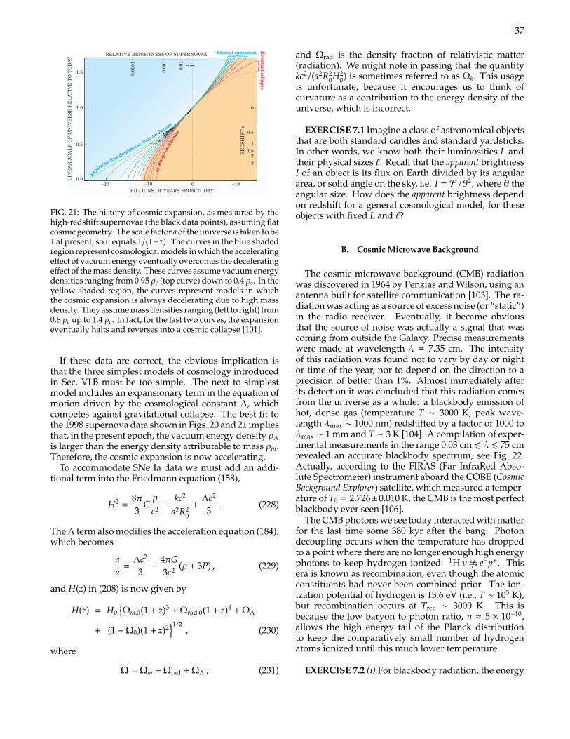
37

cosmological models, the expansion history of the cosmosis determined entirely by its mass density. The greater thedensity, the more the expansion is slowed by gravity. Thus,in the past, a high-mass-density universe would have beenexpanding much faster than it does today. So one should-n’t have to look far back in time to especially distant (faint)supernovae to find a given integrated expansion (redshift).

Conversely, in a low-mass-density universe one wouldhave to look farther back. But there is a limit to how lowthe mean mass density could be. After all, we are here, andthe stars and galaxies are here. All that mass surely putsa lower limit on how far—that is, to what level of faint-ness—we must look to find a given redshift. The high-redshift supernovae in figure 3 are, however, fainter thanwould be expected even for an empty cosmos.

If these data are correct, the obvious implication isthat the simplest cosmological model must be too simple.The next simplest model might be one that Einstein en-tertained for a time. Believing the universe to be static, hetentatively introduced into the equations of general rela-tivity an expansionary term he called the “cosmologicalconstant” (L) that would compete against gravitational col-lapse. After Hubble’s discovery of the cosmic expansion,Einstein famously rejected L as his “greatest blunder.” Inlater years, L came to be identified with the zero-pointvacuum energy of all quantum fields.

It turns out that invoking a cosmological constant al-lows us to fit the supernova data quite well. (Perhaps therewas more insight in Einstein’s blunder than in the best ef-forts of ordinary mortals.) In 1995, my SCP colleague ArielGoobar and I had found that, with a sample of type Ia su-pernovae spread over a sufficiently wide range of dis-tances, it would be possible to separate out the competingeffects of the mean mass density and the vacuum-energydensity.14

The best fit to the 1998 supernova data (see figures 3and 4) implies that, in the present epoch, the vacuum en-ergy density rL is larger than the energy density attribut-able to mass (rmc2). Therefore, the cosmic expansion is nowaccelerating. If the universe has no large-scale curvature,

as the recent measurements of the cosmic microwave back-ground strongly indicate, we can say quantitatively thatabout 70% of the total energy density is vacuum energyand 30% is mass. In units of the critical density rc, oneusually writes this result as

WL ! rL/rc " 0.7 and Wm ! rm/rc " 0.3.

Why not a cosmological constant?The story might stop right here with a happy ending—acomplete physics model of the cosmic expansion—were itnot for a chorus of complaints from the particle theorists.The standard model of particle physics has no naturalplace for a vacuum energy density of the modest magni-tude required by the astrophysical data. The simplest es-timates would predict a vacuum energy 10120 times greater.(In supersymmetric models, it’s “only” 1055 times greater.)So enormous a L would have engendered an accelerationso rapid that stars and galaxies could never have formed.Therefore it has long been assumed that there must besome underlying symmetry that precisely cancels the vac-uum energy. Now, however, the supernova data appear torequire that such a cancellation would have to leave a re-mainder of about one part in 10120. That degree of fine tun-ing is most unappealing.

The cosmological constant model requires yet anotherfine tuning. In the cosmic expansion, mass density be-comes ever more dilute. Since the end of inflation, it hasfallen by very many orders of magnitude. But the vacuumenergy density rL, a property of empty space itself, staysconstant. It seems a remarkable and implausible coinci-dence that the mass density, just in the present epoch, iswithin a factor of 2 of the vacuum energy density.

Given these two fine-tuning coincidences, it seemslikely that the standard model is missing some funda-mental physics. Perhaps we need some new kind of accel-erating energy—a “dark energy” that, unlike L, is not con-stant. Borrowing from the example of the putative“inflaton” field that is thought to have triggered inflation,theorists are proposing dynamical scalar-field models andother even more exotic alternatives to a cosmological con-

http://www.physicstoday.org April 2003 Physics Today 57

LIN

EA

R S

CA

LE

OF

UN

IVE

RSE

RE

LA

TIV

E T

O T

OD

AY1.5

1.0

0.5

0.0–20 –10 0 +10

BILLIONS OF YEARS FROM TODAY

RELATIVE BRIGHTNESS OF SUPERNOVAE

0.00

01

0.00

1

0.01 0.

11

0

0.5

11.5

23

RE

DSH

IFT

z

Eternal expansion Eventual collapse

. .. o

ral

way

sde

cele

rate

s

. .. o

ral

way

sde

cele

rate

s

Ex

pan

a

s

en ac

i

decrates, th

ot

n f sir

ce

ele

ler tes

Ex

pan

a

s

en ac

i

decrates, th

ot

n f sir

ce

ele

ler tes

Figure 4. The history of cosmic expansion, as measured by thehigh-redshift supernovae (the blackdata points), assuming flat cosmicgeometry. The scale factor R of theuniverse is taken to be 1 at pres-ent, so it equals 1/(1 + z). Thecurves in the blue shaded regionrepresent cosmological models inwhich the accelerating effect ofvacuum energy eventually over-comes the decelerating effect ofthe mass density. These curves as-sume vacuum energy densitiesranging from 0.95 rc (top curve)down to 0.4 rc. In the yellowshaded region, the curves repre-sent models in which the cosmicexpansion is always deceleratingdue to high mass density. They as-sume mass densities ranging (left toright) from 0.8 rc up to 1.4 rc. Infact, for the last two curves, the ex-pansion eventually halts and re-verses into a cosmic collapse.

FIG. 21: The history of cosmic expansion, as measured by thehigh-redshift supernovae (the black data points), assuming flatcosmic geometry. The scale factor a of the universe is taken to be1 at present, so it equals 1/(1+z). The curves in the blue shadedregion represent cosmological models in which the acceleratingeffect of vacuum energy eventually overcomes the deceleratingeffect of the mass density. These curves assume vacuum energydensities ranging from 0.95 ρc (top curve) down to 0.4 ρc. In theyellow shaded region, the curves represent models in whichthe cosmic expansion is always decelerating due to high massdensity. They assume mass densities ranging (left to right) from0.8 ρc up to 1.4 ρc. In fact, for the last two curves, the expansioneventually halts and reverses into a cosmic collapse [101].

If these data are correct, the obvious implication isthat the three simplest models of cosmology introducedin Sec. VI B must be too simple. The next to simplestmodel includes an expansionary term in the equation ofmotion driven by the cosmological constant Λ, whichcompetes against gravitational collapse. The best fit tothe 1998 supernova data shown in Figs. 20 and 21 impliesthat, in the present epoch, the vacuum energy density ρΛ

is larger than the energy density attributable to mass ρm.Therefore, the cosmic expansion is now accelerating.

To accommodate SNe Ia data we must add an addi-tional term into the Friedmann equation (158),

H2 =8π3

Gρ

c2 −kc2

a2R20

+Λc2

3. (228)

The Λ term also modifies the acceleration equation (184),which becomes

aa

=Λc2

3−

4πG3c2 (ρ + 3P) , (229)

and H(z) in (208) is now given by

H(z) = H0

Ωm,0(1 + z)3 + Ωrad,0(1 + z)4 + ΩΛ

+ (1 −Ω0)(1 + z)21/2

, (230)

where

Ω = Ωm + Ωrad + ΩΛ , (231)

and Ωrad is the density fraction of relativistic matter(radiation). We might note in passing that the quantitykc2/(a2R2

0H20) is sometimes referred to as Ωk. This usage

is unfortunate, because it encourages us to think ofcurvature as a contribution to the energy density of theuniverse, which is incorrect.

EXERCISE 7.1 Imagine a class of astronomical objectsthat are both standard candles and standard yardsticks.In other words, we know both their luminosities L andtheir physical sizes `. Recall that the apparent brightnessI of an object is its flux on Earth divided by its angulararea, or solid angle on the sky, i.e. I = F /θ2, where θ theangular size. How does the apparent brightness dependon redshift for a general cosmological model, for theseobjects with fixed L and `?

B. Cosmic Microwave Background

The cosmic microwave background (CMB) radiationwas discovered in 1964 by Penzias and Wilson, using anantenna built for satellite communication [103]. The ra-diation was acting as a source of excess noise (or “static”)in the radio receiver. Eventually, it became obviousthat the source of noise was actually a signal that wascoming from outside the Galaxy. Precise measurementswere made at wavelength λ = 7.35 cm. The intensityof this radiation was found not to vary by day or nightor time of the year, nor to depend on the direction to aprecision of better than 1%. Almost immediately afterits detection it was concluded that this radiation comesfrom the universe as a whole: a blackbody emission ofhot, dense gas (temperature T ∼ 3000 K, peak wave-length λmax ∼ 1000 nm) redshifted by a factor of 1000 toλmax ∼ 1 mm and T ∼ 3 K [104]. A compilation of exper-imental measurements in the range 0.03 cm . λ . 75 cmrevealed an accurate blackbody spectrum, see Fig. 22.Actually, according to the FIRAS (Far InfraRed Abso-lute Spectrometer) instrument aboard the COBE (CosmicBackground Explorer) satellite, which measured a temper-ature of T0 = 2.726±0.010 K, the CMB is the most perfectblackbody ever seen [106].

The CMB photons we see today interacted with matterfor the last time some 380 kyr after the bang. Photondecoupling occurs when the temperature has droppedto a point where there are no longer enough high energyphotons to keep hydrogen ionized: 1Hγ / e−p+. Thisera is known as recombination, even though the atomicconstituents had never been combined prior. The ion-ization potential of hydrogen is 13.6 eV (i.e., T ∼ 105 K),but recombination occurs at Trec ∼ 3000 K. This isbecause the low baryon to photon ratio, η ≈ 5 × 10−10,allows the high energy tail of the Planck distributionto keep the comparatively small number of hydrogenatoms ionized until this much lower temperature.

EXERCISE 7.2 (i) For blackbody radiation, the energy

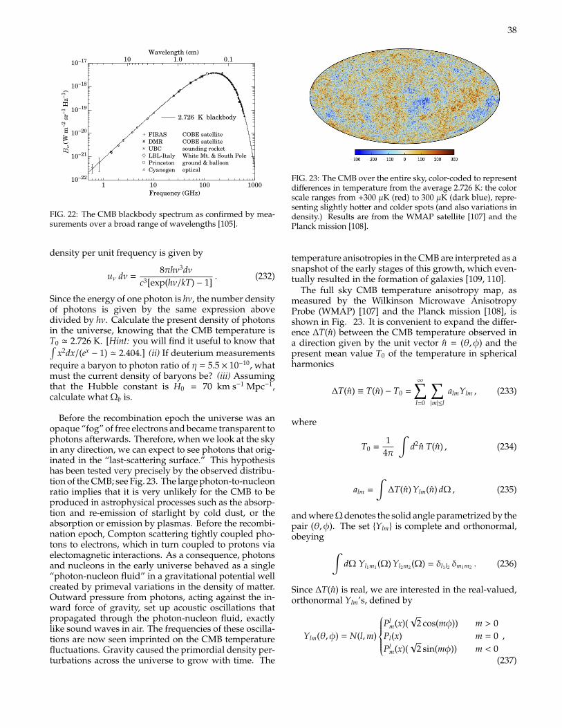
382

10−17

10−18

10−19

10−20

10−21

10−22

101 100 1000

10 1.0 0.1Wavelength (cm)

Frequency (GHz)

FIRASDMRUBCLBL-ItalyPrincetonCyanogen

COBE satelliteCOBE satellitesounding rocketWhite Mt. & South Poleground & balloonoptical

2.726 K blackbody

I ν (W

m−2

sr−

1 H

z−1)

Figure 1. Precise measurements of the CMB spectrum. The line represents a 2.73 Kblackbody, which describes the spectrum very well, especially around the peak of inten-sity. The spectrum is less well constrained at frequencies of 3 GHz and below (10 cmand longer wavelengths). (References for this figure are at the end of this section under“CMB Spectrum References.”)

1010.1 100 1000Frequency (GHz)

1.5

2.0

2.5

3.0

3.5

Wavelength (cm)30300 3 0.3 0.03

Planck

Compton y

Chemical potential µ

Free-free

Tem

per

atu

re (K

)

Figure 2. The shapes of expected, but so far unobserved, CMB distortions, resultingfrom energy-releasing processes at different epochs.

B

FIG. 22: The CMB blackbody spectrum as confirmed by mea-surements over a broad range of wavelengths [105].

density per unit frequency is given by

uν dν =8πhν3dν

c3[exp(hν/kT) − 1]. (232)

Since the energy of one photon is hν, the number densityof photons is given by the same expression abovedivided by hν. Calculate the present density of photonsin the universe, knowing that the CMB temperature isT0 ' 2.726 K. [Hint: you will find it useful to know that∫

x2dx/(ex− 1) ' 2.404.] (ii) If deuterium measurements

require a baryon to photon ratio of η = 5.5 × 10−10, whatmust the current density of baryons be? (iii) Assumingthat the Hubble constant is H0 = 70 km s−1 Mpc−1,calculate what Ωb is.

Before the recombination epoch the universe was anopaque “fog” of free electrons and became transparent tophotons afterwards. Therefore, when we look at the skyin any direction, we can expect to see photons that orig-inated in the “last-scattering surface.” This hypothesishas been tested very precisely by the observed distribu-tion of the CMB; see Fig. 23. The large photon-to-nucleonratio implies that it is very unlikely for the CMB to beproduced in astrophysical processes such as the absorp-tion and re-emission of starlight by cold dust, or theabsorption or emission by plasmas. Before the recombi-nation epoch, Compton scattering tightly coupled pho-tons to electrons, which in turn coupled to protons viaelectomagnetic interactions. As a consequence, photonsand nucleons in the early universe behaved as a single“photon-nucleon fluid” in a gravitational potential wellcreated by primeval variations in the density of matter.Outward pressure from photons, acting against the in-ward force of gravity, set up acoustic oscillations thatpropagated through the photon-nucleon fluid, exactlylike sound waves in air. The frequencies of these oscilla-tions are now seen imprinted on the CMB temperaturefluctuations. Gravity caused the primordial density per-turbations across the universe to grow with time. The

FIG. 23: The CMB over the entire sky, color-coded to representdifferences in temperature from the average 2.726 K: the colorscale ranges from +300 µK (red) to 300 µK (dark blue), repre-senting slightly hotter and colder spots (and also variations indensity.) Results are from the WMAP satellite [107] and thePlanck mission [108].

temperature anisotropies in the CMB are interpreted as asnapshot of the early stages of this growth, which even-tually resulted in the formation of galaxies [109, 110].

The full sky CMB temperature anisotropy map, asmeasured by the Wilkinson Microwave AnisotropyProbe (WMAP) [107] and the Planck mission [108], isshown in Fig. 23. It is convenient to expand the differ-ence ∆T(n) between the CMB temperature observed ina direction given by the unit vector n = (θ, φ) and thepresent mean value T0 of the temperature in sphericalharmonics

∆T(n) ≡ T(n) − T0 =

∞∑l=0

∑|m|≤l

almYlm , (233)

where

T0 =1

4π

∫d2n T(n) , (234)

alm =

∫∆T(n) Ylm(n) dΩ , (235)

and where Ω denotes the solid angle parametrized by thepair (θ, φ). The set Ylm is complete and orthonormal,obeying ∫

dΩ Yl1m1 (Ω) Yl2m2 (Ω) = δl1l2 δm1m2 . (236)

Since ∆T(n) is real, we are interested in the real-valued,orthonormal Ylm’s, defined by

Ylm(θ, φ) = N(l,m)

Pl

m(x)(√

2 cos(mφ)) m > 0Pl(x) m = 0Pl

m(x)(√

2 sin(mφ)) m < 0,

(237)

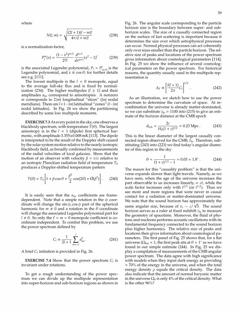
39

where

N(l,m) =

√(2l + 1)(l −m)!

4π (l + m)!(238)

is a normalization-factor,

Pml (x) =

(1 − x2)m/2

2ll!dm+l

dxm+l(x2− 1)l (239)

is the associated Legendre polynomial, Pl = Plm=0 is the

Legendre polynomial, and x ≡ cosθ; for further detailssee e.g. [111].

The lowest multipole is the l = 0 monopole, equalto the average full-sky flux and is fixed by normal-ization (234). The higher multipoles (l ≥ 1) and theiramplitudes alm correspond to anisotropies. A nonzerom corresponds to 2 |m| longitudinal “slices” (|m| nodalmeridians). There are l+1−|m| latitudinal “zones” (l−|m|nodal latitudes). In Fig. 24 we show the partitioningdescribed by some low multipole moments.

EXERCISE 7.3 At every point in the sky, one observes ablackbody spectrum, with temperature T(θ). The largestanisotropy is in the l = 1 (dipole) first spherical har-monic, with amplitude 3.355±0.008 mK [113]. The dipoleis interpreted to be the result of the Doppler shift causedby the solar system motion relative to the nearly isotropicblackbody field, as broadly confirmed by measurementsof the radial velocities of local galaxies. Show that themotion of an observer with velocity β = v/c relative toan isotropic Planckian radiation field of temperature T0produces a Doppler-shifted temperature pattern

T(θ) ≈ T0

[1 + β cosθ +

β2

2cos(2θ) + O(β3)

]. (240)

It is easily seen that the alm coefficients are frame-dependent. Note that a simple rotation in the φ coor-dinate will change the sinφ, cosφ part of the sphericalharmonic for m , 0 and a rotation in the θ coordinatewill change the associated Legendre polynomial part forl , 0. So only the ` = m = 0 monopole coefficient is co-ordinate independent. To combat this problem, we usethe power spectrum defined by

Cl ≡1

2l + 1

l∑m=−l

a2lm . (241)

A brief Cl initiation is provided in Fig. 26.

EXERCISE 7.4 Show that the power spectrum Cl isinvariant under rotations.

To get a rough understanding of the power spec-trum we can divide up the multipole representationinto super-horizon and sub-horizon regions as shown in

Fig. 26. The angular scale corresponding to the particlehorizon size is the boundary between super- and sub-horizon scales. The size of a causally connected regionon the surface of last scattering is important because itdetermines the size over which astrophysical processescan occur. Normal physical processes can act coherentlyonly over sizes smaller than the particle horizon. The rel-ative size of peaks and locations of the power spectrumgives information about cosmological parameters [114].In Fig. 25 we show the influence of several cosmolog-ical parameters on the power spectrum. For historicalreasons, the quantity usually used in the multipole rep-resentation is

∆T ≡

[l(l + 1)

2πCl

]1/2

. (242)

As an illustration, we sketch how to use the powerspectrum to determine the curvature of space. At re-combination the universe is already matter-dominated,so we can substitute zls ' 1100 into (215) to give an esti-mate of the horizon distance at the CMB epoch

dh,ls =2c

H0(1 + z)3/2≈ 0.23 Mpc . (243)

This is the linear diameter of the largest causally con-nected region observed for the CMB, `ls. Therefore, sub-stituting (243) into (223) we find today’s angular diame-ter of this region in the sky

θ =1

(1 + z)1/2 − 1= 0.03 ≈ 1.8 . (244)

The reason for this “causality problem” is that the uni-verse expands slower than light travels. Namely, as wehave seen, when the age of the universe increases thepart observable to us increases linearly, ∝ ct, while thescale factor increases only with t2/3 (or t1/2). Thus wesee more and more regions that were never in causalcontact for a radiation or matter-dominated universe.We note that the sound horizon has approximately thesame angular size, because of vs ∼ c/

√3. The sound

horizon serves as a ruler at fixed redshift zls to measurethe geometry of spacetime. Moreover, the fluid of pho-tons and nucleons performs acoustic oscillations with itsfundamental frequency connected to the sound horizonplus higher harmonics. The relative size of peaks andlocations then gives information about cosmological pa-rameters. The first panel of Fig. 25 shows that, for a flatuniverse (Ωtot ≈ 1, the first peak sits at θ ≈ 1 as we havefound in our simple estimate (244). In Fig. 25 we dis-play a compilation of measurements of the CMB angularpower spectrum. The data agree with high significancewith models when they input dark energy as providing≈ 70% of the energy in the universe, and when the totalenergy density ρ equals the critical density. The dataalso indicate that the amount of normal baryonic matterin the universe Ωb is only 4% of the critical density. Whatis the other 96%?

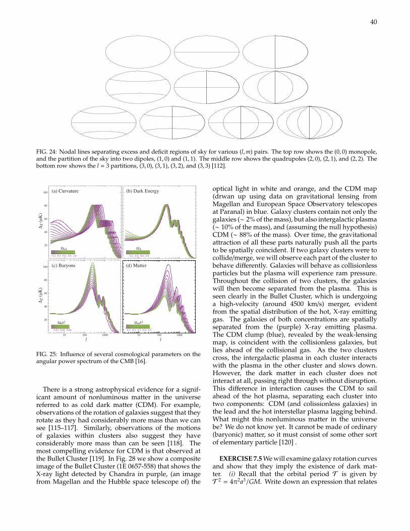
40

FIG. 24: Nodal lines separating excess and deficit regions of sky for various (l,m) pairs. The top row shows the (0, 0) monopole,and the partition of the sky into two dipoles, (1, 0) and (1, 1). The middle row shows the quadrupoles (2, 0), (2, 1), and (2, 2). Thebottom row shows the l = 3 partitions, (3, 0), (3, 1), (3, 2), and (3, 3) [112]. 16.5 Inflation

ΩΛ

0.2 0.4 0.6 0.8

20

40

60

80

100

∆T(µK)

Ωtot

0.2 0.4 0.6 0.8 1.0

Ωbh2

10

0.02 0.04 0.06

100 1000

20

40

60

80

100

l

∆T(µK)

10 100 1000

l

Ωmh2

0.1 0.2 0.3 0.4 0.5

(a) Curvature (b) Dark Energy

(c) Baryons (d) Matter

Figure 16.4: The influence of several cosmological parameters on the angular power spectrumof the CMB.

is the distance a photon travelled freely after its last scattering at tls. Thus the maximalangular separation of a causally connected points is with l = ctls(1 + zls)

ϑ =(1 + zls)tls

t0≈ 0.02 ≈ 1 (16.13)

The reason for this “causality problem” is that the universe expands slower than lighttravels: As the age of the universe increases, the part observable to us increases linearly, ∝ ct,while the scale factor increases only with t2/3 or (t1/2). Thus we see more and more regionsthat were never in causal contact for a radiation or matter-dominated universe.

The sound horizon has approximately the same angular size, because of vs ≈ c/√

3. Theexact size depends among other on the cosmological model: The sound horizon serves as aruler at fixed redshift zls to measure the geometry of space-time. Moreover, the fluid of pho-tons and nucleons performs acoustic oscillations with its fundamental frequency connectedto the sound horizon plus higher harmonics. The relative size of peaks and locations givesinformation about cosmological parameters. Figure 16.4 shows the influence of several cos-mological parameters on the angular power spectrum as function of ℓ ∼ π/ϑ. The first panelshows that the first peak sits indeed at ℓ ≈ 100 (or ϑ ∼ 1) for a flat Universe, as we havefound in our simple estimate (16.13). Observations by the WMAP satellite confirm with highsignificance the value for Ωb from BBN, for ΩΛ from type Ia supernovae, and that we live ina flat Universe.

16.5 Inflation

Shortcomings of the standard big-bang model• Causality or horizon problem: why are even causally disconnected regions of the universe

homogeneous, as we discussed for CMB?

137

FIG. 25: Influence of several cosmological parameters on theangular power spectrum of the CMB [16].

There is a strong astrophysical evidence for a signif-icant amount of nonluminous matter in the universereferred to as cold dark matter (CDM). For example,observations of the rotation of galaxies suggest that theyrotate as they had considerably more mass than we cansee [115–117]. Similarly, observations of the motionsof galaxies within clusters also suggest they haveconsiderably more mass than can be seen [118]. Themost compelling evidence for CDM is that observed atthe Bullet Cluster [119]. In Fig. 28 we show a compositeimage of the Bullet Cluster (1E 0657-558) that shows theX-ray light detected by Chandra in purple, (an imagefrom Magellan and the Hubble space telescope of) the

optical light in white and orange, and the CDM map(drwan up using data on gravitational lensing fromMagellan and European Space Observatory telescopesat Paranal) in blue. Galaxy clusters contain not only thegalaxies (∼ 2% of the mass), but also intergalactic plasma(∼ 10% of the mass), and (assuming the null hypothesis)CDM (∼ 88% of the mass). Over time, the gravitationalattraction of all these parts naturally push all the partsto be spatially coincident. If two galaxy clusters were tocollide/merge, we will observe each part of the cluster tobehave differently. Galaxies will behave as collisionlessparticles but the plasma will experience ram pressure.Throughout the collision of two clusters, the galaxieswill then become separated from the plasma. This isseen clearly in the Bullet Cluster, which is undergoinga high-velocity (around 4500 km/s) merger, evidentfrom the spatial distribution of the hot, X-ray emittinggas. The galaxies of both concentrations are spatiallyseparated from the (purple) X-ray emitting plasma.The CDM clump (blue), revealed by the weak-lensingmap, is coincident with the collisionless galaxies, butlies ahead of the collisional gas. As the two clusterscross, the intergalactic plasma in each cluster interactswith the plasma in the other cluster and slows down.However, the dark matter in each cluster does notinteract at all, passing right through without disruption.This difference in interaction causes the CDM to sailahead of the hot plasma, separating each cluster intotwo components: CDM (and colissionless galaxies) inthe lead and the hot interstellar plasma lagging behind.What might this nonluminous matter in the universebe? We do not know yet. It cannot be made of ordinary(baryonic) matter, so it must consist of some other sortof elementary particle [120] .

EXERCISE 7.5 We will examine galaxy rotation curvesand show that they imply the existence of dark mat-ter. (i) Recall that the orbital period T is given byT

2 = 4π2a3/GM. Write down an expression that relates

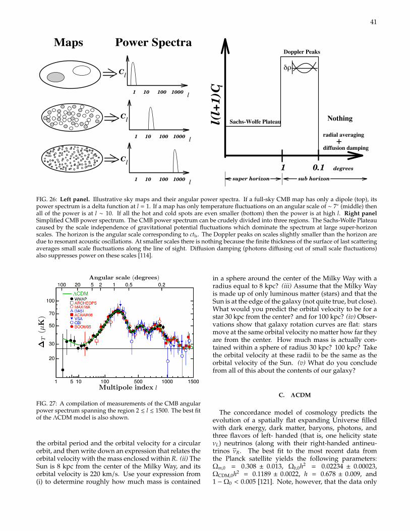
41

l(l+

1)C l

Nothing

+radial averaging

diffusion damping

Sachs-Wolfe Plateau

= constantδφ

δρ

sub horizon

0.11 super horizon

degrees

Doppler Peaks

Figure 4. Simplified CMB Power Spectrum. The CMB power spectrum

can be crudely divided into three regions. The Sachs-Wolfe Plateau caused by the

scale independence of gravitational potential fluctuations which dominate the spec-

trum at large super-horizon scales. The horizon is the angular scale corresponding

to ctdec where c is the speed of light and tdec is the age of the Universe at decou-

pling. The Doppler peaks on scales slightly smaller than the horizon are due to

resonant acoustic oscillations analogous to mellifluous bathroom singing (see Figure

8). At smaller scales there is nothing because the finite thickness of the surface of

last scattering averages small scale fluctuations along the line of sight. Di↵usion

damping (photons di↵using out of small scale fluctuations) also suppresses power

on these scales.

.

8

• the composition of the Universe: f(B,CDM ,HDM , ,)

• the origin of structure

What makes these parameters even more important and what makes CMB-cosmology such a hot subject is that in the near future measurements of the CMBangular power spectrum will determine these parameters with the unprecedentedprecision of a few % (Jungman et al. 1996).

lC

1 1000 l10010

lC

1 1000 l10010

lC

1 1000 l10010

Power SpectraMaps

Figure 2. Simple Maps and their Power Spectra. If a full-sky CMB map

has only a dipole (top), it’s power spectrum is a delta function at ` = 1 . If a map

has only temperature fluctuations on an angular scale of 7 (middle) then all of

the power is at ` 10. If all the hot and cold spots are even smaller (bottom) then

the power is at high `.

3. What is the CMB power spectrum?

Similar to the way sines and cosines are used in Fourier decompositions of arbi-trary functions on flat space, spherical harmonics can be used to make decompo-sitions of arbitrary functions on the sphere. Thus the CMB temperature maps

5

FIG. 26: Left panel. Illustrative sky maps and their angular power spectra. If a full-sky CMB map has only a dipole (top), itspower spectrum is a delta function at l = 1. If a map has only temperature fluctuations on an angular scale of ∼ 7 (middle) thenall of the power is at l ∼ 10. If all the hot and cold spots are even smaller (bottom) then the power is at high l. Right panelSimplified CMB power spectrum. The CMB power spectrum can be crudely divided into three regions. The Sachs-Wolfe Plateaucaused by the scale independence of gravitational potential fluctuations which dominate the spectrum at large super-horizonscales. The horizon is the angular scale corresponding to ctls. The Doppler peaks on scales slightly smaller than the horizon aredue to resonant acoustic oscillations. At smaller scales there is nothing because the finite thickness of the surface of last scatteringaverages small scale fluctuations along the line of sight. Diffusion damping (photons diffusing out of small scale fluctuations)also suppresses power on these scales [114].

Angular scale (degrees)

Multipole index `

T

(µK

)

l

FIG. 27: A compilation of measurements of the CMB angularpower spectrum spanning the region 2 . l . 1500. The best fitof the ΛCDM model is also shown.

the orbital period and the orbital velocity for a circularorbit, and then write down an expression that relates theorbital velocity with the mass enclosed within R. (ii) TheSun is 8 kpc from the center of the Milky Way, and itsorbital velocity is 220 km/s. Use your expression from(i) to determine roughly how much mass is contained

in a sphere around the center of the Milky Way with aradius equal to 8 kpc? (iii) Assume that the Milky Wayis made up of only luminous matter (stars) and that theSun is at the edge of the galaxy (not quite true, but close).What would you predict the orbital velocity to be for astar 30 kpc from the center? and for 100 kpc? (iv) Obser-vations show that galaxy rotation curves are flat: starsmove at the same orbital velocity no matter how far theyare from the center. How much mass is actually con-tained within a sphere of radius 30 kpc? 100 kpc? Takethe orbital velocity at these radii to be the same as theorbital velocity of the Sun. (v) What do you concludefrom all of this about the contents of our galaxy?

C. ΛCDM

The concordance model of cosmology predicts theevolution of a spatially flat expanding Universe filledwith dark energy, dark matter, baryons, photons, andthree flavors of left- handed (that is, one helicity stateνL) neutrinos (along with their right-handed antineu-trinos νR. The best fit to the most recent data fromthe Planck satellite yields the following parameters:Ωm,0 = 0.308 ± 0.013, Ωb,0h2 = 0.02234 ± 0.00023,ΩCDM,0h2 = 0.1189 ± 0.0022, h = 0.678 ± 0.009, and1 −Ω0 < 0.005 [121]. Note, however, that the data only

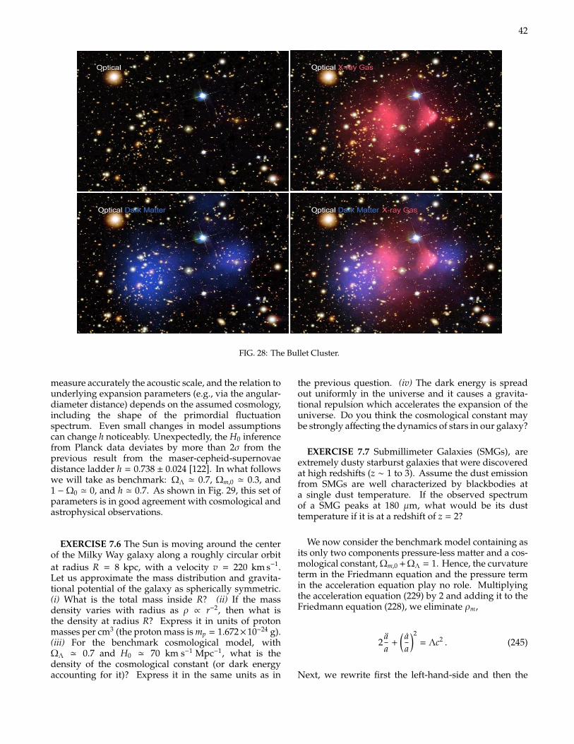
42

FIG. 28: The Bullet Cluster.

measure accurately the acoustic scale, and the relation tounderlying expansion parameters (e.g., via the angular-diameter distance) depends on the assumed cosmology,including the shape of the primordial fluctuationspectrum. Even small changes in model assumptionscan change h noticeably. Unexpectedly, the H0 inferencefrom Planck data deviates by more than 2σ from theprevious result from the maser-cepheid-supernovaedistance ladder h = 0.738 ± 0.024 [122]. In what followswe will take as benchmark: ΩΛ ' 0.7, Ωm,0 ' 0.3, and1 −Ω0 ' 0, and h ' 0.7. As shown in Fig. 29, this set ofparameters is in good agreement with cosmological andastrophysical observations.

EXERCISE 7.6 The Sun is moving around the centerof the Milky Way galaxy along a roughly circular orbitat radius R = 8 kpc, with a velocity v = 220 km s−1.Let us approximate the mass distribution and gravita-tional potential of the galaxy as spherically symmetric.(i) What is the total mass inside R? (ii) If the massdensity varies with radius as ρ ∝ r−2, then what isthe density at radius R? Express it in units of protonmasses per cm3 (the proton mass is mp = 1.672×10−24 g).(iii) For the benchmark cosmological model, withΩΛ ' 0.7 and H0 ' 70 km s−1 Mpc−1, what is thedensity of the cosmological constant (or dark energyaccounting for it)? Express it in the same units as in

the previous question. (iv) The dark energy is spreadout uniformly in the universe and it causes a gravita-tional repulsion which accelerates the expansion of theuniverse. Do you think the cosmological constant maybe strongly affecting the dynamics of stars in our galaxy?

EXERCISE 7.7 Submillimeter Galaxies (SMGs), areextremely dusty starburst galaxies that were discoveredat high redshifts (z ∼ 1 to 3). Assume the dust emissionfrom SMGs are well characterized by blackbodies ata single dust temperature. If the observed spectrumof a SMG peaks at 180 µm, what would be its dusttemperature if it is at a redshift of z = 2?

We now consider the benchmark model containing asits only two components pressure-less matter and a cos-mological constant, Ωm,0 + ΩΛ = 1. Hence, the curvatureterm in the Friedmann equation and the pressure termin the acceleration equation play no role. Multiplyingthe acceleration equation (229) by 2 and adding it to theFriedmann equation (228), we eliminate ρm,

2aa

+( a

a

)2= Λc2 . (245)

Next, we rewrite first the left-hand-side and then the

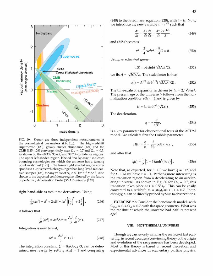
43

No Big Bang

1 2 0 1 2 3

expands forever

-1

0

1

2

3

2

3

closed

recollapses eventually

Supernovae

CMB Boomerang

Maxima

Clusters

mass density

vacu

um e

nerg

y de

nsity

(cos

mol

ogic

al c

onst

ant)

open

flat

SNAP Target Statistical Uncertainty

FIG. 29: Shown are three independent measurements ofthe cosmological parameters (ΩΛ,Ωm). The high-redshiftsupernovae [123], galaxy cluster abundance [124] and theCMB [125, 126] converge nicely near ΩΛ = 0.7 and Ωm = 0.3,as shown by the 68.3%, 95.4%, and 99.7% confidence regions.The upper-left shaded region, labeled “no big bang,” indicatesbouncing cosmologies for which the universe has a turningpoint in its past [127]. The lower right shaded region corre-sponds to a universe which is younger than long-lived radioac-tive isotopes [128], for any value of H0 ≥ 50 km s−1 Mpc−1.Alsoshown is the expected confidence region allowed by the futureSuperNova / Acceleration Probe (SNAP) mission [129].

right-hand-side as total time derivatives. Using

ddt

(aa2) = a3 + 2aaa = aa2

[( aa

)2+ 2

aa

], (246)

it follows that

ddt

(aa2) = aa2Λc2 =Λc2

3ddt

(a3) . (247)

Integration is now trivial,

aa2 =Λc2

3a3 + C . (248)

The integration constant, C = 8πGρm,0/3, can be deter-mined most easily by setting a(t0) = 1 and comparing

(248) to the Friedmann equation (228), with t = t0. Now,we introduce the new variable x = a3/2 such that

dadt

=dxdt

dadx

=dxdt

2x−1/3

3, (249)

and (248) becomes

x2−

34

Λc2x2 +94C = 0 . (250)

Using an educated guess,

x(t) = A sinh(√

3Λct/2) , (251)

we fix A =√

3C/Λc. The scale factor is then

a(t) = A2/3 sinh2/3(√

3Λc2t/2) . (252)

The time-scale of expansion is driven by tΛ = 2/√

3Λc2.The present age of the universe t0 follows from the nor-malization condition a(t0) = 1 and is given by

t0 = tΛ tanh−1(√

ΩΛ) . (253)

The deceleration,

q = −a

aH2 , (254)

is a key parameter for observational tests of the ΛCDMmodel. We calculate first the Hubble parameter

H(t) =aa

=2

3tΛcoth(t/tΛ) , (255)

and after that

q(t) =12

[1 − 3 tanh2(t/tΛ)

]. (256)

Note that, as expected, for t → 0 we have q = 1/2, andfor t → ∞ we have q = −1. Perhaps more interesting isthe transition region from a decelerating to an acceler-ating universe. As shown in Fig. 30 for ΩΛ = 0.7, thistransition takes place at t ≈ 0.55 t0. This can be easilyconveretd to a redshift: z∗ = a(t0)/a(t∗) − 1 ≈ 0.7. Inter-estingly, z∗ can be directly probed by SNe Ia observations.

EXERCISE 7.8 Consider the benchmark model, withΩm,0 ' 0.3, ΩΛ ' 0.7, with flat space geometry. What wasthe redshift at which the universe had half its presentage?

VIII. HOT THERMAL UNIVERSE

Though we can see only as far as the surface of last scat-tering, in recent decades a convincing theory of the originand evolution of the early universe has been developed.Most of this theory is based on recent theoretical andexperimental advances in elementary particle physics.

4415.6 The ΛCDM model

-1

-0.8

-0.6

-0.4

-0.2

0

0.2

0.4

0.6

0 0.5 1 1.5 2

q

t/t0

Ω=0.9

Ω=0.1

Figure 15.3: The deceleration parameter q as function of t/t0 for a ΛCDM model and variousvalues for ΩΛ (0.1, 0.3, 0.5, 0.7 and 0.9 from the top to the bottom).

The limiting behavior of q corresponds with q = 1/2 for t → 0 and q = −1 for t → ∞ asexpected to the one of a flat Ωm = 1 and a ΩΛ = 1 universe. More interesting is the transitionregion and, as shown in Fig. 15.3, the transition from a decelerating to an accelerating universehappens for ΩΛ = 0.7 at t ≈ 0.55t0. This can easily converted to redshift, z∗ = a(t0)/a(t∗) −1 ≈ 0.7, that is directly measured by Supernova observations.

Exercises

1. Derive the relation between temperature and time in the early (radiation dominated)universe using ρ = gaT 4 = gπ2T 4/30 as expression for the energy density of a gas withg relativistic degrees of freedom in the Friedmann equation. What is the temperatureat t = 1 s? [Hints: The expression ρ = gπ2T 4/30 is valid for k = c = ! = 1. Then onecan measure temperatures in MeV/GeV and use s−1 = 6.6 × 10−25 GeV and G−1/2 =MPl = 1.2 × 1019 GeV.]

129

t/t0

q(t) = 0.1

= 0.9

FIG. 30: The deceleration parameter q as a function oft/t0 for the ΛCDM model for various values of ΩΛ =0.1, 0.3, 0.5, 0.7, 0.9 from top to bottom [16].

Hence, before continuing our look back through time,we make a detour to overview the generalities of thestandard model of particle physics.2

A. SU(3)C ⊗ SU(2)L ⊗U(1)Y

The standard model (SM) is our most modern attemptto answer two simple questions that have been perplex-ing (wo)mankind throughout the epochs: What is theUniverse made of? Why is our world the way it is?

The elementary-particle model accepted today viewsquarks and leptons as the basic (pointlike) constituentsof ordinary matter. By pointlike, we understand thatquarks and leptons show no evidence of internal struc-ture at the current limit of our resolution. Presently,the world’s largest microscope is the Large Hadron Col-lider (or LHC), a machine that collides beams of protonsat a cenetr-of-mass energy

√s = 13 TeV. Remarkably,

70% of the energy carried into the collision by the pro-tons emerges perpendicular to the incident beams. Ata given transverse energy E⊥, we may roughly estimatethe LHC resolution as

`LHC ≈ c/E⊥ ≈ 2 × 10−19 TeV m/E⊥≈ 2 × 10−20 m . (257)

There are six quarks and six leptons, together with theirantiparticles. These twelve elementary particles are allspin- 1

2 and fall naturally into three families or gener-ations. Each generation consists of two leptons withelectric charges Q = 0 and Q = −1 and two quarks with

2 You can find a more extensive but still qualitative discussion in [13].For a more rigorous treatment see e.g. [130–133].

Q = +2/3 and Q = −1/3. The masses of the particles in-crease significantly with each generation, with the pos-sible exception of the neutrinos [134]. The properties ofquarks and leptons are summarized in Table I.

Now, an understanding of how the world is put to-gether requires a theory of how quarks and leptons inter-act with one another. Equivalently, it requires a theoryof the fundamental forces of nature. Four such forceshave been identified. They can be characterized on thebasis of the following four criteria: the types of parti-cles that experience the force, the relative strength of theforce, the range over which the force is effective, andthe nature of the particles that mediate the force. Twoof the forces, gravitation and electromagnetism, have anunlimited range; largely for this reason they are famil-iar to everyone. The remaining forces, which are calledsimply the weak force and the strong force, cannot beperceived directly because their influence extends onlyover a short range, no larger than the radius of an atomicnucleus. The electromagnetic force is carried by the pho-ton, the strong force is mediated by gluons, the W and Zbosons transmit the weak force, and the quantum of thegravitational force is called the graviton. The main prop-erties of the force carriers are summarized in Table II. Acomparison of the (approximate) relative force strengthsfor two protons inside a nucleus is given in Table III.Though gravity is the most obvious force in daily life, ona nuclear scale it is the weakest of the four forces and itseffect at the particle level can nearly always be ignored.

In the SM quarks and leptons are allotted several addi-tive quantum numbers: electric charge Q, lepton num-ber L = Le + Lµ + Lτ, baryon number B, strangeness s,charmness c, bottomness b, and topness t. For each par-ticle additive quantum number N, the correspondingantiparticle has the additive quantum number −N.

The additive quantum numbers Q and B are assumedto be conserved in strong, electromagnetic, and weakinteractions. The lepton numbers are not involved instrong interactions, but are strictly conserved in bothelectromagnetic and weak interactions. The remainder,s, c, b and t are strictly conserved only in strong andelectromagnetic interactions, but can undergo a changeof one unit in weak interactions.

The quarks have an additional charge which enablesthem to interact strongly with one another. This chargeis a three-fold degree of freedom which has come tobe known as color [135], and so the gauge theory de-scribing the strong interaction has taken on the nameof quantum chromodynamics (QCD). Each quark flavorcan have three colors usually designated red, green, andblue. The antiquarks are colored antired, antigreen, andantiblue. Each quark or antiquark carries a single unitof color or anticolor charge, respectively. The quanta ofthe color fields are called gluons (as they glue the quarkstogether). There are eight independent kinds of gluonsin SU(3)C, each of which carries a combination of a colorcharge and an anticolor charge (e.g. red-antigreen). Thestrong interactions between color charges are such that

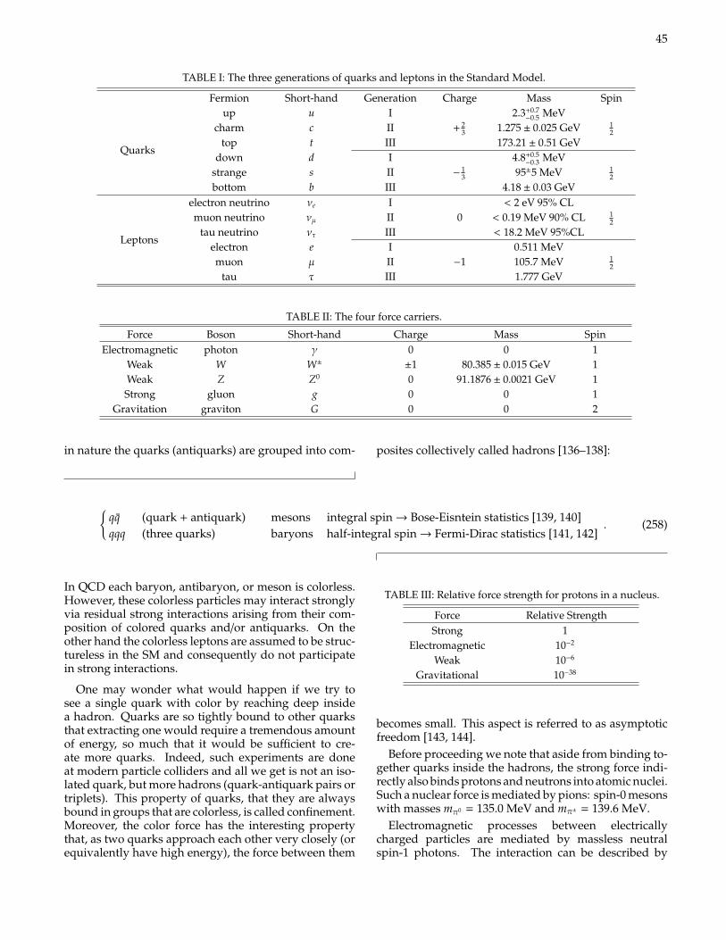
45

TABLE I: The three generations of quarks and leptons in the Standard Model.

Fermion Short-hand Generation Charge Mass Spin

Quarks

up u I 2.3+0.7−0.5 MeV

charm c II + 23 1.275 ± 0.025 GeV 1

2

top t III 173.21 ± 0.51 GeVdown d I 4.8+0.5

−0.3 MeVstrange s II −

13 95±5 MeV 1

2

bottom b III 4.18 ± 0.03 GeV

Leptons

electron neutrino νe I < 2 eV 95% CLmuon neutrino νµ II 0 < 0.19 MeV 90% CL 1

2

tau neutrino ντ III < 18.2 MeV 95%CLelectron e I 0.511 MeVmuon µ II −1 105.7 MeV 1

2

tau τ III 1.777 GeV

TABLE II: The four force carriers.

Force Boson Short-hand Charge Mass SpinElectromagnetic photon γ 0 0 1

Weak W W±±1 80.385 ± 0.015 GeV 1

Weak Z Z0 0 91.1876 ± 0.0021 GeV 1Strong gluon g 0 0 1

Gravitation graviton G 0 0 2

in nature the quarks (antiquarks) are grouped into com- posites collectively called hadrons [136–138]:

qq (quark + antiquark) mesons integral spin→ Bose-Eisntein statistics [139, 140]qqq (three quarks) baryons half-integral spin→ Fermi-Dirac statistics [141, 142]

. (258)

In QCD each baryon, antibaryon, or meson is colorless.However, these colorless particles may interact stronglyvia residual strong interactions arising from their com-position of colored quarks and/or antiquarks. On theother hand the colorless leptons are assumed to be struc-tureless in the SM and consequently do not participatein strong interactions.

One may wonder what would happen if we try tosee a single quark with color by reaching deep insidea hadron. Quarks are so tightly bound to other quarksthat extracting one would require a tremendous amountof energy, so much that it would be sufficient to cre-ate more quarks. Indeed, such experiments are doneat modern particle colliders and all we get is not an iso-lated quark, but more hadrons (quark-antiquark pairs ortriplets). This property of quarks, that they are alwaysbound in groups that are colorless, is called confinement.Moreover, the color force has the interesting propertythat, as two quarks approach each other very closely (orequivalently have high energy), the force between them

TABLE III: Relative force strength for protons in a nucleus.

Force Relative StrengthStrong 1

Electromagnetic 10−2

Weak 10−6

Gravitational 10−38

becomes small. This aspect is referred to as asymptoticfreedom [143, 144].

Before proceeding we note that aside from binding to-gether quarks inside the hadrons, the strong force indi-rectly also binds protons and neutrons into atomic nuclei.Such a nuclear force is mediated by pions: spin-0 mesonswith masses mπ0 = 135.0 MeV and mπ± = 139.6 MeV.

Electromagnetic processes between electricallycharged particles are mediated by massless neutralspin-1 photons. The interaction can be described by

46

a local U(1)EM gauge theory called quantum electro-dynamics (QED). The symmetry properties of QEDare unquestionably appealing [145–151]. Moreover,QED has yielded results that are in agreement withexperiment to an accuracy of about one part in abillion [152], which makes the theory the most accuratephysical theory ever devised. It is the model for theoriesof the other fundamental forces and the standard bywhich such theories are judged.

Every quark and lepton of the SM interact weakly. Theweak interaction, mediated by the massive W+, W− andZ0 vector bosons, fall into two classes: (i) charge-current(CC) weak interactions involving the W+ and W− bosonsand (ii) neutral current (NC) weak interactions involvingthe Z0 boson. The CC interactions, acting exclusively onleft-handed particles and right-handed antiparticles, aredescribed by a chiral SU(2)L local gauge theory, wherethe subscript L refers to left-handed particles only.3 Onthe other hand, the NC interactions act on both left-handed and right-handed particles, similar to the elec-tromagnetic interactions. In fact the SM assumes thatboth the Z0 and the photon arise from a mixing of twobosons, W0 and B0, via the electroweak mixing angle θW :

γ = B0 cosθW + W0 sinθW ,

Z0 = −B0 sinθW + W0 cosθW . (259)

The electroweak interaction is described by a local gaugetheory: SU(2)L ⊗ U(1)Y, where the hypercharge U(1)Ysymmetry involves both left-handed and right-handedparticles [153–155]. Experiment requires the masses ofthe weak gauge bosons W and Z to be heavy so that weakinteractions are very short-ranged. The W and Z gaugebosons acquire masses through spontaneous symmetrybreaking SU(2)L × U(1)Y → U(1)EM. The breaking ofthe symmetry triggers the Higgs mechanism [156, 157],which gives the relative masses of the W and Z bosonsin terms of the electroweak mixing angle,

MW = MZ cosθW , (260)

while the photon remains massless. In addition, by cou-pling originally massless fermions to the scalar Higgsfield, it is possible to produce the observed physicalfermion masses without violating the gauge invariance.

The conspicuously well-known accomplishments ofthe SU(3)C ⊗ SU(2)L ⊗ U(1)Y SM of strong and elec-troweak forces can be considered as the apotheosis of thegauge symmetry principle to describe particle interac-tions. Most spectacularly, the recent discovery [158, 159]of a new boson with scalar quantum numbers and cou-plings compatible with those of a SM Higgs has possibly

3 A phenomenon is said to be chiral if it is not identical to its mirrorimage. The spin of a particle may be used to define a handednessfor that particle. The chirality of a particle is right-handed if thedirection of its spin is the same as the direction of its motion. It isleft-handed if the directions of spin and motion are opposite.

plugged the final remaining experimental hole in the SM,cementing the theory further.

In summary, the fundamental particles can be classi-fied into spin-1/2 fermions (6 leptons and 6 quarks), andspin-1 gauge bosons (γ, W±,Z0, and g). The leptons have18 degrees of freedom: each of the 3 charged leptonshas 2 possible chiralities and its associated anti-particle,whereas the 3 neutrinos and antineutrinos have onlyone chirality (neutrinos are left-handed and antineutri-nos are right-handed). The quarks have 72 degrees offreedom: each of the 6 quarks, has the associated an-tiparticle, three different color states, and 2 chiralities.The gauge bosons have 27 degrees of freedom: a photonhas two possible polarization states, each massive gaugeboson has 3, and each of the eight independent types ofgluon in QCD has 2. The scalar spin-0 Higgs boson, witha mass mH ' 126 GeV, has 1 degree of freedom.4

B. Equilibrium thermodynamics

The Universe we observe had its beginning in the bigbang, the cosmic firewall. Because the early universe wasto a good approximation in thermal equilibrium, particlereactions can be modeled using the tools of thermody-

4 Recently, ATLAS [160] and CMS [161] announced the observationof a peak in the diphoton mass distribution around 750 GeV, using(respectively) 3.2 fb−1 and 2.6 fb−1 of data recorded at a c.m. en-ergy

√s = 13 TeV. The diphoton excesses could be interpreted as

the decay products of a new massive particle z, with spin 0, 2, orhigher [162]. Assuming a narrow width approximation ATLAS givesa local significance of 3.6σ, or else a global significance of 2.0σwhenthe look-elsewhere-effect in the mass range Mz/GeV ∈ [200 − 2000]is accounted for. Signal-plus-background fits were also imple-mented for a broad signal component with a large decay width. Thelargest deviation from the background-only hypothesis correspondsto Mz ∼ 750 GeV with a total width Γtotal ∼ 45 GeV. The local andglobal significances evaluated for the broad resonance fit are roughly0.3 higher than that for the fit using the narrow width approximation,corresponding to 3.9σ and 2.3σ, respectively. The CMS data gives alocal significance of 2.6σ and a global significance smaller than 1.2σ.More recently, ATLAS and CMS updated their diphoton resonancesearches [163–165]. ATLAS reanalyzed the 3.2 fb−1 of data, targetingseparately spin-0 and spin-2 resonances. For spin-0, the most signif-icant deviation from the background-only hypothesis correspondsto Mz ∼ 750 GeV and Γtotal ∼ 45 GeV. The local significance is nowincreased to 3.9σ but the global significance remains at the 2σ level.For the spin-2 resonance, both the local and global significances arereduced down to 3.6σ and 1.8σ, respectively. The new CMS analysisincludes additional data (recorded in 2015 while the magnet was notoperated) for a total of 3.3 fb−1. The largest excess is observed forMz = 760 GeV and Γtotal ≈ 11 GeV, and has a local significance of 2.8σfor spin-0 and 2.9σ spin-2 hypothesis. After taking into account theeffect of searching for several signal hypotheses, the significance ofthe excess is reduced to < 1σ. CMS also communicated a combinedsearch with data recorded at

√s = 13 TeV and

√s = 8 TeV. For the

combined analysis, the largest excess is observed at Mz = 750 GeVand Γtotal = 0.1 GeV. The local and global significances are ≈ 3.4σand 1.6σ, respectively. This could be the first observation of physicsbeyond the SM at the LHC.

47

namics and statistical mechanics. It will be helpfull thento take a second detour and revise some concepts of sta-tistical thermodynamics.

Consider a cubic box of volume V, and expand thefields inside into periodic waves with harmonic bound-ary conditions. The density of states in k-space is

dN = gV

(2π)3 d3k , (261)

where g is a degeneracy factor and k is the Fourier trans-form wavenumber. The equilibrium phase space distri-bution (or occupancy) function for a quantum state ofenergy E is given by the familiar Fermi-Dirac or Bose-Einstein distrubutions,

f =1

e(E−µ)/(kT) ± 1, (262)

where T is the equilibrium temperature, k is the Boltz-mann constant, µ is the chemical potential (if present),and ± corresponds to either Fermi or Bose statistics.Throughout we will consider the case |µ| T and ne-glect all chemical potentials when computing total ther-modynamic quantities. All evidence indicates that thisis a good approximation to describe particle interactionsin the super-hot primeval plasma [166] .

The number density of a dilute weakly-interacting gasof particles in thermal equilibrium with g internal de-grees of freedom is then

n =1V

∫f dN

= g1

(2π)3

∫∞

0

4πp2dpeE/(kT) ± 1

= g1

2π23c3

∫∞

mc2

(E2−m2c3)1/2

eE/(kT) ± 1E dE , (263)

where in the second line we have changed to momentumspace, ~p = ~k, and in the third line we used the relativisticrelation E = m2c4+p2c2. The analogous expression for theenergy density is easily obtain since it is only necessaryto multiply the integrand in (263) by a factor of E for theenergy of each mode,

ρ =g

2π23c3

∫∞

mi

(E2−m2c4)1/2

eE/(kT) ± 1E2 dE . (264)

Recalling that the pressure is the average value of themomentum transfer 〈p〉2c2/E in a given direction, wehave

P =g

6π23c3

∫∞

mi

(E2−m2c4)3/2

eE/(kT) ± 1dE , (265)

with the factor of 1/3 associated with the assumedisotropy of the momentum distribution.

Let us now compute the above expressions in twoasymptotic limits: relativistic and non-relativistic par-ticles, which will be sufficient for our discussion of

how the different particle species evolve in the primevalplasma. For kT mc2, the particles behave as if theywere massless and the Bose-Einstein and Fermi-Diracdistributions reduce to

f (y) =1

ey ± 1, (266)

where we have defined y = |~p |/(kT). Using∫∞

0

zn−1

ez − 1dz = Γ(n) ζ(n) (267)

and ∫∞

0

zn−1

ez + 1dz =

12n (2n

− 2) Γ(n) ζ(n) , (268)

we obtain

n =

(kTc

)3 4πg(2π)3

∫∞

0

y2dyey ± 1

= A±ζ(3)π2 g

(kTc

)3

,

ρ = B±π2g

30(c)3 (kT)4 ,

P =13ρ , (269)

where ζ(3) ≈ 1.2 and A− = 1 for bosons, and A+ =3/4 for fermions, B− = 1 for bosons and B+ = 7/8 forfermions.5

For kT mc2, the exponential factor dominates thedenominator in both the Bose-Einstein and Fermi-Diracdistributions in (262), so that the bosonic or fermionicnature of the particles becomes indistinguishable. Fur-thermore, we have

E = (p2c2 + m2c4)1/2 = mc2

(1 +

p2

m2c2

)1/2

' mc2 +p2

2m. (270)

Defining x = |~p |/√

2mkT, for the number density weobtain the Boltzmann distribution

n = e−mc2/(kT)(2mkT)3/2 4πg(2π)3

∫∞

0e−x2

x2dx

=g3

(mkT2π

)3/2

e−mc2/(kT) , (271)

5 The Gamma function is an extension of the factorial function fornon-integer and complex numbers. If s is a positive integer, thenΓ(s) = (s−1)!. The Riemann zeta function of a real variable s, definedby the infinite series ζ(s) =

∑∞

n=1 1/ns, converges ∀s > 1. Note that(268) follows from (267) using the relation 1

ex+1 = 1ex−1 −

2e2x−1

.

48

where we have used∫∞

0xne−x2

dx =12

Γ(1 + n

2

), (272)

with n = 2 and Γ(3/2) =√π/2. From (270) it is easily

seen that to leading order ρ = mc2n in this case.To obtain the associated pressure, note that to leading

order |p2c2|/E ' |p|2/m, so that

P ' e−mc2/(kT)(2mkT)5/2 4πg(2π)3

13m

∫∞

0x4e−x2

dx

= e−mc2/(kT)(2mkT)5/2 4πg(2π)3

13m

3√π

8

=g3

(mkT2π

)3/2

e−mc2/(kT) kT

= nkT , (273)

where we have used Γ(5/2) = 3√π/4. Note that (273)

is just but the familar result for a non-relativistic perfectgas, P = nkT. Since kT mc2, we have P ρ and thepressure may be neglected for a gas of non-relativisticparticles, as we had anticipated.

For a gas of non-degenerate, relativistic species, theaverage energy per particle is

〈E〉 =ρ

n=

π4k30ζ(3) T ' 2.701 T for bosons

7π4k180ζ(3) T ' 3.151 T for fermions

, (274)

whereas for a non-relativistic species

〈E〉 = mc2 +32

kT . (275)

The internal energy U can be considered to be a func-tion of two thermodynamic variables among P, V , andT. (These variables are related by the equation of state.)Let us choose V and T to be the fundamental variables.The internal energy can then be written as U(V,T). Letus differentiate this function:

dU =

(∂U∂V

)T

dV +

(∂U∂T

)V

dT . (276)

This equation can be combined with the first law (167)to give

TdS =

[(∂U∂V

)T

+ P]

dV +

(∂U∂T

)V

dT . (277)

Now, since the internal energy is a function of T and Vwe may therefore choose to view S as a function of T andV, and this gives rise to the differential relation

dS =

(∂S∂T

)V

dT +

(∂S∂V

)T

dV . (278)

Substituting (278) into (277) and equating the dV and dTparts gives the familiar

∂U∂T

= T∂S∂T

(279)

and

S =U + PV

T, (280)

where we have used the relation for extensive quatities(∂S/∂V = S/V and ∂U/∂V).6 It is useful to define theentropy density s = S/V, which is thus given by

s = ρ + P . (281)

For photons, we can compute all of the thermody-namic quantities rather easily

nγ =2ζ(3)π2

(kTγc3

)= 60.42

(kThc

)3

= 20.28(T

K

)3

photons cm−3 ,

ργ =π2

15(kTγ)4

(c)3 = 0.66(kTγ)4

(c)3 ,

〈Eγ〉 =ρ

n= 3.73 × 1016

( TK

)erg ,

Pγ =13ργ ,

sγ =43ργTγ. (282)

In the limit kT mic2, the total energy density can beconveniently expressed by

ρrad =

∑B

gB +78

∑F

gF

1(c)3

π2

30(kT)4

=1

(c)3

π2

30gρ(T) (kT)4 , (283)

where gB(F) is the total number of boson (fermion)degrees of freedom and the sum runs over all boson(fermion) states with mic2

kT. The factor of 7/8 is dueto the difference between the Fermi and Bose integrals.(283) defines the effective number of degrees of freedom,gρ(T), by taking into account new particle degrees offreedom as the temperature is raised. The change ingρ(T) (ignoring mass effects) is given in Table IV [167].

6 Recall that an extensive property is any property that depends on thesize (or extent) of the system under consideration. Take two identicalsamples with all properties identical and combine them into a singlesample. Properties that double (e.g., energy, volume, entropy) areextensive. Properties that remain the same (e.g., temperature andpressure) are intensive.

49

TABLE IV: Effective numbers of degrees of freedom in SM.

Temperature New particles 4gρ(T)

T < me γ’s + ν’s 29me < T < mµ e± 43mµ < T < mπ µ± 57mπ < T < T∗c π’s 69Tc < T < mcharm - π’s + u, u, d, d, s, s + gluons 247mc < T < mτ c, c 289mτ < T < mbottom τ± 303mb < T < mW,Z b, b 345mW,Z < T < mHiggs W±,Z 381mH < T < mtop H0 385mt < T t, t 427

*Tc corresponds to the confinement–deconfinement transitionbetween quarks and hadrons.

At higher temperatures, gρ(T) will be model dependent.

EXERCISE 8.1 If in the next 1010 yr the volume of theuniverse increases by a factor of two, what then will bethe temperature of the blackbody radiation?

C. The first millisecond

The history of the universe from 10−10 seconds to todayis based on observational facts: the fundamental lawsof high energy physics are well-established up to theenergies reached by the LHC. Before 10−10 seconds, theenergy of the universe exceeds 13 TeV and we lose thecomfort of direct experimental guidance. The physicsof that era is therefore as speculative as it is fascinating.Herein we will go back to the earliest of times - as closeas possible to the big bang - and follow the evolution ofthe Universe.

It is cear that as a→ 0 the temperature increases with-out limit T → ∞, but there comes a point at which theextrapolation of classical physics breaks down. This isthe realm of quantum black holes, where the thermalenergy of typical particles of mass m is such that their deBroglie wavelength is smaller than their Schwarzschildradius. Equating h/mc to 2Gm/c2 yields a characteristicmass for quantum gravity known as the Planck massMPl.7 This mass scale, together with the correspondinglength /(MPlc) and time /(MPlc2) define the system of

7 Strictly speaking this is not quite the Planck mass. It is a factor of√π larger. However, this heuristic derivation gives the right order

of magnitude.

Planck units:

MPl ≡

√cG' 1019 GeV ,

`Pl ≡

√Gc3 ' 10−35 m ,

tPl ≡

√Gc5 ' 10−43 s . (284)

The Planck time therefore sets the origin of time for theclassical big bang era. It is inaccurate to extend the classi-cal solution of Friedmann equation to a = 0 and concludethat the universe began in a singularity of infinite den-sity.

At t ∼ 10−43 s, a kind of phase transition is thought tohave occured during which the gravitational force con-densed out as a separate force. The symmetry of the fourforces was broken, but the strong, weak, and electro-magnetic forces were still unified, and there were nodistinctions between quarks and leptons. This is anunimaginably short time, and predictions can be onlyspeculative. The temperature would have been about1032 K, corresponding to particles moving about everywhich way with an average kinetic energy of

kT ≈1.4 × 10−23 J/K 1032 K

1.6 × 10−10 J/GeV≈ 1019 GeV , (285)

where we have ignored the factor 2/3 in our order ofmagnitude calculation. Very shortly thereafter, as thetemperature had dropped to about 1028 K, there wasanother phase transition and the strong force condensedout at about 10−35 s after the bang. Now the universewas filled with a soup of quarks and leptons. About thistime, the universe underwent an incredible exponentialexpansion, increasing in size by a factor of & 1026 in atiny fraction of a second, perhaps ∼ 10−34 s.

As a matter of fact, the favored ΛCDM model implic-itly includes the hypothesis of a very early period inwhich the scale factor of the universe expands exponen-tially: a(t) ∝ eHt. If the interval of exponential expansionsatisfies ∆t & 60/H, a small casually connected regioncan grow sufficiently to accommodate the observed ho-mogeneity and isotropy [168]. To properly understandwhy this is so, we express the comoving horizon (210) asan integral of the comoving Hubble radius,

%h ≡ c∫ t

0

dt′

a(t′)= c

∫ a

0

daHa2 = c

∫ a

0

1aH

d ln a . (286)

At this stage it is important to emphasize a subtle dis-tinction between the comoving horizon %h and the co-moving Hubble radius c/(aH). If particles are separatedby distances greater than %h, they never could have com-municated with one another; if they are separated bydistances greater than c/(aH), they cannot talk to eachother now. This distinction is crucial for the solution tothe horizon problem which relies on the following: It is

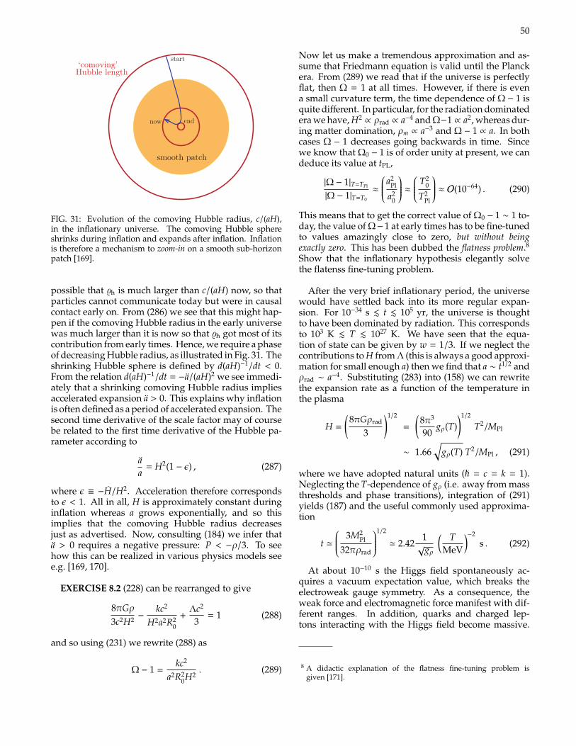
50

5.1.2 Flatness Problem Revisited

Recall the Friedmann Equation (41) for a non-flat universe

|1 (a)| =1

(aH)2. (49)

If the comoving Hubble radius decreases this drives the universe toward flatness (rather than away

from it). This solves the flatness problem! The solution = 1 is an attractor during inflation.

5.1.3 Horizon Problem Revisited

A decreasing comoving horizon means that large scales entering the present universe were inside the

horizon before inflation (see Figure 2). Causal physics before inflation therefore established spatial

homogeneity. With a period of inflation, the uniformity of the CMB is not a mystery.

‘comoving’

smooth patch

now end

Hubble lengthstart

Comoving Horizon

Time [log(a)]

Inflation Hot Big Bang

Comoving Scales

horizon exit horizon re-entry

density fluctuation

Figure 7: Left: Evolution of the comoving Hubble radius, (aH)1, in the inflationary universe. The

comoving Hubble sphere shrinks during inflation and expands after inflation. Inflation is

therefore a mechanism to ‘zoom-in’ on a smooth sub-horizon patch. Right: Solution of

the horizon problem. All scales that are relevant to cosmological observations today were

larger than the Hubble radius until a 105. However, at suciently early times, these

scales were smaller than the Hubble radius and therefore causally connected. Similarly,

the scales of cosmological interest came back within the Hubble radius at relatively recent

times.

5.2 Conditions for Inflation

Via the Friedmann Equations a shrinking comoving Hubble radius can be related to the acceleration

and the the pressure of the universe

d

dt

H1

a

< 0 ) d2a

dt2> 0 ) + 3p < 0 . (50)

The three equivalent conditions for inflation therefore are:

27

FIG. 31: Evolution of the comoving Hubble radius, c/(aH),in the inflationary universe. The comoving Hubble sphereshrinks during inflation and expands after inflation. Inflationis therefore a mechanism to zoom-in on a smooth sub-horizonpatch [169].

possible that %h is much larger than c/(aH) now, so thatparticles cannot communicate today but were in causalcontact early on. From (286) we see that this might hap-pen if the comoving Hubble radius in the early universewas much larger than it is now so that %h got most of itscontribution from early times. Hence, we require a phaseof decreasing Hubble radius, as illustrated in Fig. 31. Theshrinking Hubble sphere is defined by d(aH)−1/dt < 0.From the relation d(aH)−1/dt = −a/(aH)2 we see immedi-ately that a shrinking comoving Hubble radius impliesaccelerated expansion a > 0. This explains why inflationis often defined as a period of accelerated expansion. Thesecond time derivative of the scale factor may of coursebe related to the first time derivative of the Hubble pa-rameter according to

aa

= H2(1 − ε) , (287)

where ε ≡ −H/H2. Acceleration therefore correspondsto ε < 1. All in all, H is approximately constant duringinflation whereas a grows exponentially, and so thisimplies that the comoving Hubble radius decreasesjust as advertised. Now, consulting (184) we infer thata > 0 requires a negative pressure: P < −ρ/3. To seehow this can be realized in various physics models seee.g. [169, 170].

EXERCISE 8.2 (228) can be rearranged to give

8πGρ3c2H2 −

kc2

H2a2R20

+Λc2

3= 1 (288)

and so using (231) we rewrite (288) as

Ω − 1 =kc2

a2R20H2

. (289)

Now let us make a tremendous approximation and as-sume that Friedmann equation is valid until the Planckera. From (289) we read that if the universe is perfectlyflat, then Ω = 1 at all times. However, if there is evena small curvature term, the time dependence of Ω − 1 isquite different. In particular, for the radiation dominatedera we have, H2

∝ ρrad ∝ a−4 and Ω−1 ∝ a2, whereas dur-ing matter domination, ρm ∝ a−3 and Ω − 1 ∝ a. In bothcases Ω − 1 decreases going backwards in time. Sincewe know that Ω0 − 1 is of order unity at present, we candeduce its value at tPL,

|Ω − 1|T=TPl

|Ω − 1|T=T0

≈

a2Pl

a20

≈ T20

T2Pl

≈ O(10−64) . (290)

This means that to get the correct value of Ω0 − 1 ∼ 1 to-day, the value of Ω−1 at early times has to be fine-tunedto values amazingly close to zero, but without beingexactly zero. This has been dubbed the flatness problem.8Show that the inflationary hypothesis elegantly solvethe flatenss fine-tuning problem.

After the very brief inflationary period, the universewould have settled back into its more regular expan-sion. For 10−34 s . t . 105 yr, the universe is thoughtto have been dominated by radiation. This correspondsto 103 K . T . 1027 K. We have seen that the equa-tion of state can be given by w = 1/3. If we neglect thecontributions to H from Λ (this is always a good approxi-mation for small enough a) then we find that a ∼ t1/2 andρrad ∼ a−4. Substituting (283) into (158) we can rewritethe expansion rate as a function of the temperature inthe plasma

H =

(8πGρrad

3

)1/2

=

(8π3

90gρ(T)

)1/2

T2/MPl

∼ 1.66√

gρ(T) T2/MPl , (291)

where we have adopted natural units ( = c = k = 1).Neglecting the T-dependence of gρ (i.e. away from massthresholds and phase transitions), integration of (291)yields (187) and the useful commonly used approxima-tion

t '

3M2Pl

32πρrad

1/2

' 2.421√gρ

( TMeV

)−2

s . (292)

At about 10−10 s the Higgs field spontaneously ac-quires a vacuum expectation value, which breaks theelectroweak gauge symmetry. As a consequence, theweak force and electromagnetic force manifest with dif-ferent ranges. In addition, quarks and charged lep-tons interacting with the Higgs field become massive.

8 A didactic explanation of the flatness fine-tuning problem isgiven [171].

51

The fundamental interactions have by then taken theirpresent forms.

By the time the universe was about a microsecond old,quarks began to condense into mesons and baryons. Tosee why, let us focus on the most familiar hadrons: nu-cleons and their antiparticles. When the average kineticenergy of particles was somewhat higher than 1 GeV,protons, neutrons, and their antiparticles were contin-ually being created out of the energies of collisions in-volving photons and other particles. But just as quickly,particle and antiparticles would annihilate. Hence theprocess of creation and annihilation of nucleons was inequilibrium. The numbers of nucleons and antinucle-ons were high: roughly as many as there were electrons,positrons, or photons. But as the universe expandedand cooled, and the average kinetic energy of particlesdropped below about 1 GeV, which is the minimum en-ergy needed in a typical collision to create nucleons andantinucleons (940 MeV each), the process of nucleon cre-ation could not continue. However, the process of anni-hilation could continue with antinucleons annihilatingnucleons, until there were almost no nucleons left; butnot quite zero!

Manned and unmanned exploration of the solar sys-tem tell us that it is made up of the same stuff as the Earth:baryons. Observational evidence from radio-astronomyand cosmic ray detection indicate that the Milky Way,as well as interstellar space, and distant galaxies are alsomade of baryons. Therefore, we can cautiously concludethat the baryon number of the observable universe isB > 0. This requires that the early qq plasma contained atiny surplus of quarks. After all anti-matter annihilatedwith matter, only the small surplus of matter remained

η =nB − nB

nγ= 5 × 10−10 excess baryons

photons. (293)

The tiny surplus can be explained by interactions in theearly universe that were not completely symmetric withrespect to an exchange of matter-antimatter, the so-called“baryogenesis” [172].

At this stage, it is worthwhile to point out that if somerelativistic particles have decoupled from the photons,it is necessary to distinguish between two kinds of rel-ativistic degrees of freedom (r.d.o.f.): those associatedwith the total energy density gρ, and those associatedwith the total entropy density gs. At energies abovethe deconfinement transition towards the quark gluonplasma, quarks and gluons are the relevant fields forthe QCD sector, such that the effective number of inter-acting (thermally coupled) r.d.o.f. is gs(T) = 61.75. Asthe universe cools down below the confinement scaleΛQCD ∼ 200 MeV, the SM plasma transitions to a regimewhere mesons and baryons are the pertinent degrees offreedom. Precisely, the relevant hadrons present in thisenergy regime are pions and charged kaons, such thatgs(T) = 19.25 [173]. This significant reduction in the de-grees of freedom results from the rapid annihilation ordecay of more massive hadrons which may have formed

during the transition. The quark-hadron crossover tran-sition therefore corresponds to a large redistribution ofentropy into the remaining degrees of freedom. To con-nect the temperature to an effective number of r.d.o.f. wemake use of some high statistics lattice simulations of aQCD plasma in the hot phase, especially the behaviorof the entropy during the changeover [174]. Concretely,the effective number of interacting r.d.o.f. in the plasmaat temperature T is given by

gs(T) ' r(T)(gB +

78

gF

), (294)

where the coefficient r(T) is unity for leptons, two forphoton contributions, and is the ratio s(T)/sSB for thequark-gluon plasma [175]. Here, s(T) and sSB are the en-tropy density and the ideal Stefan-Bolzmann limit shownin Fig 32. The entropy rise during the confinement-deconfinement changeover can be parametrized, for150 MeV < T < 500 MeV, by

sT3 '

42.82√

392πe−C1 + 18.62

C22[

eC2 − 1]2 eC2 , (295)

where C1 = (TMeV − 151)2 /392 and C2 = 195.1/(TMeV −

134). For the same energy range, we obtain

gs(T) ' 47.5 r(T) + 19.25 . (296)

In Fig. 32 we show gs(T) as given by (296). Theparametrization is in very good agreement with phe-nomenological estimates [176, 177].

The entropy density is dominated by the contributionof relativistic particles, so to a very good approximation

s =2π2

45gs(T) T3 . (297)

Conservation of S = sV leads to

ddt

(sa3) = 0 (298)

and therefore that gs(T)T3a3 remains constant as the uni-verse expands. As one would expect, a non-evolvingsystem would stay at constant number or entropy den-sity in comoving coordinates even though the numberor entropy density is in fact decreasing due to the ex-pansion of the universe. Since the quark-gluon energydensity in the plasma has a similar T dependence to thatof the entropy (see e.g. Fig. 7 in [174]), hereafter wesimplify the discussion by taking g = gρ = gs.

After the first millisecond has elapsed, when the ma-jority of hadrons and anti-hadrons annihilated eachother, we entered the lepton era.

D. Neutrino decoupling and BBN

After the first tenth of a second, when the temper-ature was about 3 × 1010 K, the universe was filled

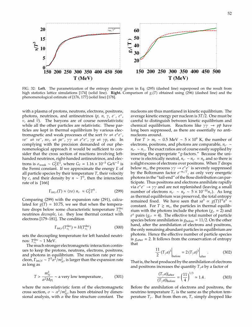
52

sSB íT3

150 200 250 300 350 400 450 5000

5

10

15

20

T HMeVL

sêT3

150 200 250 300 350 400 450 500

2030405060

T HMeVL

g sHTL

1

FIG. 32: Left. The parametrization of the entropy density given in Eq. (295) (dashed line) superposed on the result fromhigh statistics lattice simulations [174] (solid line). Right. Comparison of gs(T) obtained using (296) (dashed line) and thephenomenological estimate of [176, 177] (solid line) [178].

with a plasma of protons, neutrons, electrons, positrons,photons, neutrinos, and antineutrinos (p, n, γ, e−, e+,ν, and ν). The baryons are of course nonrelativisticwhile all the other particles are relativistic. These par-ticles are kept in thermal equilibrium by various elec-tromagnetic and weak processes of the sort νν e+e−,νe− νe−, nνe pe−, γγ e+e−, γp γp, etc. Incomplying with the precision demanded of our phe-nomenological approach it would be sufficient to con-sider that the cross section of reactions involving left-handed neutrinos, right-handed antineutrinos, and elec-trons is σweak ∼ G2

FE2, where GF = 1.16 × 10−5 GeV−2 isthe Fermi constant. If we approximate the energy E ofall particle species by their temperature T, their velocityby c, and their density by n ∼ T3, then the interactionrate of is [166]

Γint,ν(T) ≈ 〈vσ〉 nν ≈ G2FT5 . (299)

Comparing (299) with the expansion rate (291), calcu-lated for g(T) = 10.75, we see that when the tempera-ture drops below some characteristic temperature Tdec

νL

neutrinos decouple, i.e. they lose thermal contact withelectrons [179–181]. The condition

Γint,ν(TdecνL

) = H(TdecνL

) (300)

sets the decoupling temperature for left handed neutri-nos: Tdec

νL∼ 1 MeV.

The much stronger electromagnetic interaction contin-ues to keep the protons, neutrons, electrons, positrons,and photons in equilibrium. The reaction rate per nu-cleon, Γint,N ∼ T3α2/m2

N, is larger than the expansion rateas long as

T >m2

N

α2MPl∼ a very low temperature , (301)

where the non-relativistic form of the electromagneticcross section, σ ∼ α2/m2

N, has been obtained by dimen-sional analysis, with α the fine structure constant. The

nucleons are thus mantianed in kinetic equilibrium. Theaverage kinetic energy per nucleon is 3T/2. One must becareful to distinguish between kinetic equilibrium andchemical equilibrium. Reactions like γγ → pp havelong been suppressed, as there are essentially no anti-nucleons around.

For T > me ∼ 0.5 MeV ∼ 5 × 109 K, the number ofelectrons, positrons, and photons are comparable, ne− ∼

ne+ ∼ nγ. The exact ratios are of course easily supplied byinserting the appropriate “g-factors.” Because the uni-verse is electrically neutral, ne− − ne+ = np and so there isa slight excess of electrons over positrons. When T dropsbelow me, the process γγ→ e+e− is severely suppressedby the Boltzmann factor e−me/T, as only very energeticphotons in the “tail-end” of the Bose distribution can par-ticipate. Thus positrons and electrons annihilate rapidlyvia e+e− → γγ and are not replenished (leaving a smallnumber of electrons ne− ∼ np ∼ 5 × 10−10nγ). As longas thermal equilibrium was preserved, the total entropyremained fixed. We have seen that sa3

∝ g(T)T3a3 =constant. For T & me, the particles in thermal equilib-rium with the photons include the photon (gγ = 2) ande± pairs (ge± = 4). The effective total number of particlespecies before annihilation is gbefore = 11/2.On the otherhand, after the annihilation of electrons and positrons,the only remaining abundant particles in equilibrium arephotons. Hence the effective number of particle speciesis gafter = 2. It follows from the conservation of entropythat

112

(Tγa)3∣∣∣∣∣before

= 2 (Tγa)3∣∣∣∣∣after

. (302)

That is, the heat produced by the annihilation of electronsand positrons increases the quantity Tγa by a factor of

(Tγa)|after

(Tγa)|before=

(114

)1/3

' 1.4 . (303)

Before the annihilation of electrons and positrons, theneutrino temperature Tν is the same as the photon tem-perature Tγ. But from then on, Tν simply dropped like

53

a−1, so for all subsequent times, Tνa equals the valuebefore annihilation,

(Tνa)|after = (Tνa)|before = (Tγa)|before . (304)

We conclude therefore that after the annihilation pro-cess is over, the photon temperature is higher than theneutrino temperature by a factor of(

TγTν

)∣∣∣∣∣∣after

=(Tγa)|after

(Tνa)|after' 1.4 . (305)

Therefore, even though out of thermal equilibrium,the neutrinos and antineutrinos make an importantcontribution to the energy density.

EXERCISE 8.3 By assuming that neutrinos saturatethe dark matter density derive an upper bound on theneutrino mass [182].

The energy density stored in relativistic species is customarily given in terms of the so-called effective number ofneutrino species, Neff , through the relation

ρrad =

[1 +

78

( 411

)4/3

Neff

]ργ , (306)

and so

Neff ≡

(ρrad − ργ

ρν

)'

87

∑B

′ gB

2

(TB

Tν

)4

+∑

F

′ gF

2

(TF

Tν

)4

, (307)

whereρν denotes the energy density of a single species of massless neutrinos, TB(F) is the effective temperature of boson(fermion) species, and the primes indicate that electrons and photons are excluded from the sums [183, 184]. Thenormalization of Neff is such that it gives Neff = 3 for three families of massless left-handed standard model neutrinos.For most practical purposes, it is accurate enough to consider that neutrinos freeze-out completely at about 1 MeV.However, as the temperature dropped below this value, neutrinos were still interacting with the electromagneticplasma and hence received a tiny portion of the entropy from pair annihilations. The non-instantaneous neutrinodecoupling gives a correction to the normalization Neff = 3.046 [185–188].

Near 1 MeV, the CC weak interactions,

nνe pe−, ne+ pνe, n pe−νe (308)

guarantee neutron-proton chemical equilibrium. Defining λnp as the summed rate of the reactions which convertneutrons to protons,

λnp = λ(nνe → pe−) + λ(ne+→ pνe) + λ(n→ pe−νe) , (309)

the rate λpn for the reverse reactions which convert protons to neutrons is given by detailed balance:

λpn = λnp e−∆m/T(t), (310)

where ∆m ≡ mn −mp = 1.293 MeV. The evolution of the fractional neutron abundance Xn/N ≡ nn/nN is described bythe balance equation

dXn/N(t)dt

= λpn(t)[1 − Xn/N(t)] − λnp(t)Xn/N(t) , (311)

where nN is the total nucleon density at this time, nN = nn + np. The equilibrium solution is obtained by settingdXn/N(t)/dt = 0:

Xeqn/N(t) =

λpn(t)λpn(t) + λnp(t)

=[1 + e∆m/T(t)

]−1. (312)

The neutron abundance tracks its value in equilibrium until the inelastic neutron-proton scattering rate decreasessufficiently so as to become comparable to the Hubble expansion rate. At this point the neutrons freeze-out, that isthey go out of chemical equilibrium. The neutron abundance at the freeze-out temperature TFO

n/N = 0.75 MeV can beapproximated by its equilibrium value (312),

Xn/N(TFOn/N) ' Xeq

n/N(TFOn/N) =

[1 + e∆m/TFO

n/N

]−1. (313)

54

Since the ratio ∆m/TFOn/N is of O(1), a substantial fraction of neutrons survive when chemical equilibrium between

neutrons and protons is broken.At this time, the photon temperature is already below the deuterium binding energy ∆D ' 2.2 MeV, thus one

would expect sizable amounts of D to be formed via n p→ Dγ process. However, the large photon-nucleon densityratio η−1 delays deuterium synthesis until the photo–dissociation process become ineffective (deuterium bottleneck).Defining the onset of nucleosynthesis by the criterion

e∆D/TBBNη ∼ 1 , (314)

we obtain TBBN ≈ 89 keV. Note that (314) ensures that below TBBN the high energy tail in the photon distribution,with energy larger than ∆D, has been sufficiently diluted by the expansion. At this epoch, N(T) = 3.36, hence thetime-temperature relationship (292) dictates that big bang nucleosynthesis (BBN) begins at

tBBN ' 167 s ≈ 180 s , (315)

as widely popularized by Weinberg [22].Once D starts forming, a whole nuclear process network sets in [189, 190]. When the temperature dropped below∼ 80 keV, the universe has cooled sufficiently that the cosmic nuclear reactor can begin in earnest, building thelightest nuclides through the following sequence of two-body reactions

p n→ γD,p D→3Heγ, D D→3He n, D D→ p T,TD→4He n, 4He T→7Liγ,3He n→ p T, 3He D→4He p, 3He 4He→7Beγ,7Li p→4He 4He, 7Be n→7Li p,

...

. (316)

By this time the neutron abundance surviving at freeze-out has been depleted by β-decay to

Xn/N(TBBN) ' Xn/N(TFOn/N) e−tBBN/τn , (317)

where τn ' 887 s is the neutron lifetime. Nearly all of these surviving neutrons are captured in 4He because of itslarge binding energy (∆4He = 28.3 MeV) via the reactions listed in (316). Heavier nuclei do not form in any significantquantity both because of the absence of stable nuclei with A=5 or 8, which impedes nucleosynthesis via n 4He, p 4Heor 4He 4He reactions, and because of the large Coulomb barrier for reactions such as 4He T → 7Li γ and 3He 4He→

7Be γ. By the time the temperature has dropped below ∼ 30 keV, a time comparable to the neutron lifetime, theaverage thermal energy of the nuclides and nucleons is too small to overcome the Coulomb barriers; any remainingfree neutrons decay, and BBN ceases. The resulting mass fraction of helium, conventionally referred to Yp, is simplygiven by

Yp ' 2Xn/N(tBBN) = 0.251 , (318)

where the subscript p denotes primordial. The above calculation demonstrates how the synthesized helium abun-dance depends on the physical parameters. After a bit of algebra, (318) can be rweritten as [189]

Yp ' 0.251 + 0.014 ∆Neffν + 0.0002∆τn + 0.009 ln

( η

5 × 10−10

). (319)

In summary, primordial nucleosynthesis has a singleadjustable parameter: the baryon density. Observationsthat led to the determination of primordial abundanceof D, 3He and 7Li can determine η. The internalconsistency of BBN can then be checked by comparingthe abundances of the other nuclides, predicted usingthis same value of η, with observed abundances.Interestingly, in contrast to the other light nuclides, the

BBN-predicted primordial abundance of 4He is veryinsensitive to the baryon density parameter. Rather, the4He mass fraction depends on the neutron-to-protonratio at BBN because virtually all neutrons available atthat time are incorporated into 4He. Therefore, while D,3He, and 7Li are potential baryometers, 4He provides apotential chronometer.

55

EXERCISE 8.4 Suppose that the difference in restenergy of the neutron and proton were 0.1293 MeV,instead of 1.293 MeV, with all other physical parametersunchanged. Estimate the maximum possible massfraction in 4He, assuming that all available neutrons areincorporated into 4He nuclei.

EXERCISE 8.5 A fascinating bit of cosmologicalhistory is that of Gamow’s prediction of the CMB inthe late 1940s [191–193]. Unfortunately, his predictionwas premature; by the time the CMB was actuallydiscovered, his prediction had fallen into obscurity.This problem reproduces Gamow’s line of argument.Gamow knew that nucleosynthesis must have takenplace at a temperature TBBN ≈ 109 K. He also knewthat the universe must currently be t0 ∼ 1010 yearsold. He then assumed that the universe was flat andradiation dominated, even at the present time. (i) Withthese assumptions, what was the energy density of theuniverse at the time of nucleosynthesis? (ii) What wasthe Hubble parameter at the time of nucleosynthesis?(c) What was the age of the universe at BBN? (iv) Giventhe present age, what should the present temperatureof the CMB be? (v) If we then assume that the universechanged from being radiation dominated to matterdominated at a redshift zeq > 0, will this increase ordecrease the CMB temperature, for fixed values of TBBNand t0?

The observationally-inferred primordial fractionsof baryonic mass in 4He (Yp = 0.2472 ± 0.0012,Yp = 0.2516 ± 0.0011, Yp = 0.2477 ± 0.0029, andYp = 0.240 ± 0.006) [194–196] have been constantlyfavoring Neff

ν . 3 [197]. Unexpectedly, two recent inde-pendent studies yield Yp values somewhat higher thanprevious estimates: Yp = 0.2565±0.001(stat)±0.005(syst)and Yp = 0.2561 ± 0.011 [198–200]. For τn = 885.4 ± 0.9 sand τn = 878.5 ± 0.8 s, the updated effectivenumber of light neutrino species is reported asNeff = 3.68+0.80

−0.70 (2σ) and Neff = 3.80+0.80−0.70 (2σ), re-

spectively. The most recent estimate of Yp yieldsNeff = 3.58 ± 0.25(68%CL),±0.40(95.4%CL),±(99%CL).This entails that a non-standard value of Neff is preferredat the 99% CL, implying the possible existence ofadditional types of neutrino species [201].

EXERCISE 8.6 We have seen that he best multi-parameter fit of Planck data yields a Hubble constantwhich deviates by more than 2σ from the value obtainedwith the HST. The impact of the Planck h estimate is par-ticularly important in the determination of Neff . Com-bining observations of CMB data the Planck Collabora-tion reported Neff = 3.15 ± 0.23 [121]. However, if thevalue of h is not allowed to float in the fit, but instead isfrozen to the value determined from the maser-cepheid-supernovae distance ladder, the Planck CMB data thengives Neff = 3.62 ± 0.25, which suggests new neutrino-like physics (at around the 2.3σ level) [202]. The hints

of extra relativistic degrees of freedom at BBN and CMBepochs can be explained, e.g., by means of the right-handed partners of the three, left-handed, SM neutrinos.In particular, milli-weak interactions of these Dirac statesmay allow the νR’s to decouple much earlier, at a highertemperature, than their left-handed counterparts [203].Determine the minimum decoupling temperature of theright-handed neutrinos which is consistent with Planckdata at the 1σ level.

E. Quantum black holes

As we have seen, black holes are the evolutionary end-points of massive stars that undergo a supernova explo-sion leaving behind a fairly massive burned out stellarremnant. With no outward forces to oppose gravita-tional forces, the remnant will collapse in on itself.

The density to which the matter must be squeezedscales as the inverse square of the mass. For example,the Sun would have to be compressed to a radius of 3 km(about four millionths its present size) to become a blackhole. For the Earth to meet the same fate, one would needto squeeze it into a radius of 9 mm, about a billionth itspresent size. Actually, the density of a solar mass blackhole (∼ 1019 kg/m3) is about the highest that can be cre-ated through gravitational collapse. A body lighter thanthe Sun resists collapse because it becomes stabilized byrepulsive quantum forces between subatomic particles.

However, stellar collapse is not the only way to formblack holes. The known laws of physics allow matterdensities up to the so-called Planck value 1097 kg/m3,the density at which the force of gravity becomes sostrong that quantum mechanical fluctuations can breakdown the fabric of spacetime, creating a black hole witha radius ∼ 10−35 m and a mass of 10−8 kg. This is thelightest black hole that can be produced according to theconventional description of gravity. It is more massivebut much smaller in size than a proton.

The high densities of the early universe were a pre-requisite for the formation of primordial black holes butdid not guarantee it. For a region to stop expanding andcollapse to a black hole, it must have been denser than av-erage, so the density fluctuations were also necessary. Aswe have seen, such fluctuations existed, at least on largescales, or else structures such as galaxies and clustersof galaxies would never have coalesced. For primordialblack holes to form, these fluctuations must have beenstronger on smaller scales than on large ones, which ispossible though not inevitable. Even in the absence offluctuations, holes might have formed spontaneously atvarious cosmological phase transitions – for example,when the universe ended its early period of acceleratedexpansion, known as inflation, or at the nuclear densityepoch, when particles such as protons condensed out ofthe soup of their constituent quarks.

The realization that black holes could be so smallprompted Stephen Hawking to consider quantum ef-

56

fects, and in 1974 his studies lead to the famous conclu-sion that black holes not only swallow particles but alsospit them out [204, 205]. The strong gravitational fieldsaround the black hole induce spontaneous creation ofpairs near the event horizon. While the particle withpositive energy can escape to infinity, the one with neg-ative energy has to tunnel through the horizon into theblack hole where there are particle states with negativeenergy with respect to infinity.9 As the black holes ra-diate, they lose mass and so will eventually evaporatecompletely and disappear. The evaporation is generallyregarded as being thermal in character,10 with a temper-ature inversely proportional to its mass MBH,

TBH =1

8πGMBH=

14 π rs

, (320)

and an entropy S = 2πMBH rs, where rs is theSchwarzschild radius and we have set c = 1. Note thatfor a solar mass black hole, the temperature is around10−6 K, which is completely negligible in today’s uni-verse. But for black holes of 1012 kg the temperature isabout 1012 K hot enough to emit both massless particles,such as γ-rays, and massive ones, such as electrons andpositrons.

The black hole, however, produces an effective po-tential barrier in the neighborhood of the horizon thatbackscatters part of the outgoing radiation, modifing theblackbody spectrum. The black hole absorption crosssection, σs (a.k.a. the greybody factor), depends uponthe spin of the emitted particles s, their energy Q, andthe mass of the black hole [210]. At high frequencies(Qrs 1) the greybody factor for each kind of particlemust approach the geometrical optics limit. The inte-grated power emission is reasonably well approximatedtaking such a high energy limit. Thus, for illustrativesimplicity, in what follows we adopt the geometric op-tics approximation, where the black hole acts as a perfectabsorber of a slightly larger radius, with emitting areagiven by [210]

A = 27πr2s . (321)

Within this framework, we can conveniently write thegreybody factor as a dimensionless constant normalizedto the black hole surface area seen by the SM fields Γs =σs/A4, such that Γs=0 = 1, Γs=1/2 ≈ 2/3, and Γs=1 ≈ 1/4.

All in all, a black hole emits particles with initial totalenergy between (Q,Q + dQ) at a rate

dNi

dQ=

σs

8π2 Q2[exp

( QTBH

)− (−1)2s

]−1

(322)

9 One can alternatively think of the emitted particles as coming fromthe singularity inside the black hole, tunneling out through the eventhorizon to infinity [206].

10 Indeed both the average number [204, 205] and the probability dis-tribution of the number [207–209] of outgoing particles in each modeobey a thermal spectrum.

per degree of particle freedom i. The change of variablesu = Q/T, brings Eq. (322) into a more familar form,

Ni =27 Γs TBH

128π3

∫u2

eu − (−1)2s du. (323)

This expression can be easily integrated using (267) and(268), and yields

Ni = A±27 Γs

128π3 Γ(3) ζ(3) TBH . (324)

Therefore, the black hole emission rate is found to be

Ni ≈ 7.8 × 1020( TBH

GeV

)s−1 , (325)

Ni ≈ 3.8 × 1020( TBH

GeV

)s−1 , (326)

Ni ≈ 1.9 × 1020( TBH

GeV

)s−1 , (327)

for particles with s = 0, 1/2, 1, respectively.At any given time, the rate of decrease in the black

hole mass is just the total power radiated

dMBH

dQ= −

∑i

giσs

8π2

Q3

eQ/TBH − (−1)2s , (328)

where gi is the number of internal degrees of freedom ofparticle species i. A straightforward calculation gives

MBH = −∑

i

gi B±27 Γs

128π3 Γ(4) ζ(4) T2BH . (329)

Assuming that the effective high energy theory containsapproximately the same number of modes as the SM (i.e.,gs=1/2 = 90, and gs=1 = 27), we find

dMBH

dt= 8.3 × 1073 GeV4 1

M2BH

. (330)

Ignoring thresholds, i.e., assuming that the mass of theblack hole evolves according to (330) during the entireprocess of evaporation, we can obtain an estimate for thelifetime of the black hole,

τBH = 1.2 × 10−74 GeV−4∫

M2BH dMBH . (331)

Using = 6.58×10−25 GeV s, (331) can then be re-writtenas

τBH ' 2.6 × 10−99 (MBH/GeV)3 s' 1.6 × 10−26 (MBH/kg)3 yr . (332)

This implies that for a solar mass black hole, the lifetimeis unobservably long 1064 yr, but for a 1012 kg one, it is

57

∼ 1.5 × 1010 yr, about the present age of the universe.Therefore, any primordial black hole of this mass wouldbe completing its evaporation and exploding right now.

The questions raised by primordial black holesmotivate an empirical search for them. Most of the massof these black holes would go into gamma rays (quarksand gluons would hadronize mostly into pions whichin turn would decay to γ-rays and neutrinos), with anenergy spectrum that peaks around 100 MeV. In 1976,Hawking and Don Page realized that γ-ray backgroundobservations place strong upper limits on the numberof such black holes [211]. Specifically, by looking atthe observed γ-ray spectrum, they set an upper limitof 104/pc3 on the density of these black holes withmasses near 5 × 1011 kg. Even if primordial black holesnever actually formed, thinking about them has led toremarkable physical insights because they linked threepreviously disparate areas of physics: general relativity,quantum theory, and thermodynamics [212].

EXERCISE 8.7 Very recently, it has become evidentthat a promising route towards reconciling the apparentmismatch of the fundamental scales of particle physicsand gravity is to modify the short distance behavior ofgravity at scales much larger than the Planck length.Such modification can be most simply achieved by intro-ducing extra dimensions (generally thought to be curled-up) in the sub-millimiter range [213]. In the canonicalexample, spacetime is a direct product of ordinary 4-dimensional spacetime and a (flat) spatial n-torus withcircumferences of length 2πri (i = 1, ...,n), generally ofcommon linear size ri = rc. The SM fields cannot propa-gate freely in the extra dimensions without conflict withobservations. This is avoided by trapping the fields toa 3-dimensional brane-world. Applying Gauss’ law atr rc and r rc, it is easily seen that the effectivePlanck scale is related to the fundamental scale of grav-ity M∗ simply by a volume factor,

rc =(MPl

M∗

)2/n 1M∗

= 2.0 × 10−17(TeV

M∗

) (MPl

M∗

)2/n

cm , (333)

so that M∗ can range from ∼ TeV to 1019 GeV, forrc ≤ 1 mm and n ≥ 2. If nature gracefully picked a suffi-ciently low-scale gravity, the first evidence for it wouldlikely be the observation of microscopic black holes pro-duced in particle collisions [214]. Although the blackhole production cross section, O(M−1

W ), is about 5 ordersof magnitude smaller than QCD cross sections,O(Λ−1

QCD),it was proposed that such black holes could be producedcopiously at the LHC [215, 216] and in cosmic ray colli-sions [217, 218], and that these spectacular events couldbe easily filtered out of the QCD background. To a firstapproximation it is reasonable to assume that the evap-oration process is dominated by the large number of SMbrane modes [219, 220]. Therefore, the emission rate

per degree of particle freedom i of particles of spin swith initial total energy between (Q,Q + dQ) can be ap-proximated by (322). The characteristic temperature ofa 4 + n-dimensional black hole is [221]

TBH =n + 14π rs

, (334)

where

rs =1

M∗

MBH

M∗

2nπ(n−3)/2Γ( n+32 )

n + 2

1/(1+n)

, (335)

is the Schwarzschild radius [222]. As in the conve-tional 4-dimensional case, we can conveniently rewritethe greybody factor as a dimensionless constant, Γs =σs/A4⊂4+n, normalized to the black hole surface area

A4⊂4+n = 4π(n + 3

2

)2/(n+1) n + 3n + 1

r2s (336)

seen by the SM fields [219]. The upper limit on theaccretion rate for a 4 + n-dimensional black hole is

dMdt

∣∣∣∣∣accr≈ π

(n + 32

)2/(n+1) n + 3n + 1

r2s ε , (337)

where ε is the nearby quark-gluon (or parton) energydensity [223]. The highest earthly value of energy den-sity of partonic matter is the one created at the LHC,εLHC < 500 GeV/fm3. Consider the case with n = 6,which is well motivated by string theory [224]. (i) Showthat the black holes that could be produced at the LHC(or in any forseeable accelerator built on Earth) wouldevaporate much too quickly to swallow the partonsnearby. (ii) Determine the black hole lifetime. [Hint: Forn = 6, you can evaluate the numerical results of [225] at〈Q〉 and normalize the cross sections results to the cap-ture area A4⊂4+n to obtain Γs=1/2 ≈ 0.33 and Γs=1 ≈ 0.34.]

IX. MULTI-MESSENGER ASTRONOMY

For biological reasons our perception of the Universeis based on the observation of photons, most trivially bystaring at the night-sky with our bare eyes. Conventionalastronomy covers many orders of magnitude in pho-ton wavelengths, from 104 cm radio-waves to 10−14 cmgamma rays of GeV energy. This 60 octave span in pho-ton frequency allows for a dramatic expansion of ourobservational capacity beyond the approximately oneoctave perceivable by the human eye.

The γ-ray sky has been monitored since 1968. Thepioneering observations by the third Orbiting Solar Ob-servatory (OSO-3) provided the first γ-ray sky map,with 621 events detected above 50 MeV [226]. In ad-dition, these observations revealed the existence of anisotropic emission. The presence of an isotropic diffuseγ-ray background (IGRB) has been confirmed by the

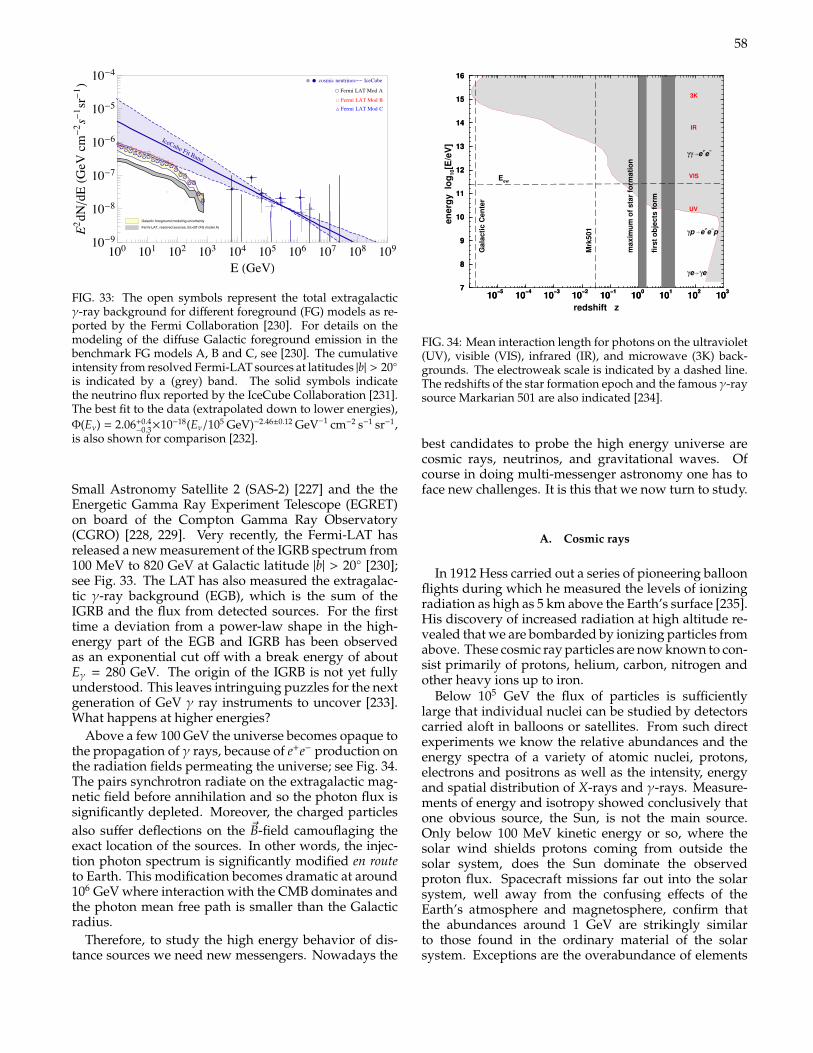
58

ÁÁÁÁÁÁÁÁÁÁÁÁÁÁÁÁÁÁÁÁÁÁÁÁ

ÁÁ

ÉÉÉÉÉÉÉÉÉÉÉÉÉÉÉÉÉÉÉÉÉÉÉÉ

ÉÉ

ÛÛÛÛÛÛÛÛÛÛÛÛÛÛÛÛÛÛÛÛÛÛÛÛ

ÛÛ

Ê

Ê

ÊÊ ÊÊ

ÊÊ

ÊÊ

100 101 102 103 104 105 106 107 108 10910-9

10-8

10-7

10-6

10-5

10-4

E HGeVL

E2dNêdEHGe

Vcm-2 s-1 sr-1 L Ê Ê cosmic neutrinos-- IceCube

Á Fermi LAT Mod A

É Fermi LAT Mod BÛ Fermi LAT Mod C

GFM Uncertainty Bands

IceCube Fit Band

– 31 –

Energy [MeV]210 310 410 510 610

]-1

sr

-1 s

-2 d

N/d

E [M

eV c

m2 E

-610

-510

-410

-310 Total EGB

Fermi LAT, 50 months, (FG model A)

Fermi LAT, 50 months, (FG model B)

Fermi LAT, 50 months, (FG model C)

Galactic foreground modeling uncertainty

(FG model A)°Fermi LAT, resolved sources, |b|>20

Fig. 8.— Comparison of the total EGB intensities for di↵erent foreground models. The total EGB

intensity is obtained by summing the IGRB intensity and the cumulative intensity from resolved

Fermi LAT sources at latitudes |b| > 20 (gray band). See Figure 7 for legend.

FIG. 33: The open symbols represent the total extragalacticγ-ray background for different foreground (FG) models as re-ported by the Fermi Collaboration [230]. For details on themodeling of the diffuse Galactic foreground emission in thebenchmark FG models A, B and C, see [230]. The cumulativeintensity from resolved Fermi-LAT sources at latitudes |b| > 20is indicated by a (grey) band. The solid symbols indicatethe neutrino flux reported by the IceCube Collaboration [231].The best fit to the data (extrapolated down to lower energies),Φ(Eν) = 2.06+0.4

−0.3×10−18(Eν/105 GeV)−2.46±0.12 GeV−1 cm−2 s−1 sr−1,is also shown for comparison [232].

Small Astronomy Satellite 2 (SAS-2) [227] and the theEnergetic Gamma Ray Experiment Telescope (EGRET)on board of the Compton Gamma Ray Observatory(CGRO) [228, 229]. Very recently, the Fermi-LAT hasreleased a new measurement of the IGRB spectrum from100 MeV to 820 GeV at Galactic latitude |b| > 20 [230];see Fig. 33. The LAT has also measured the extragalac-tic γ-ray background (EGB), which is the sum of theIGRB and the flux from detected sources. For the firsttime a deviation from a power-law shape in the high-energy part of the EGB and IGRB has been observedas an exponential cut off with a break energy of aboutEγ = 280 GeV. The origin of the IGRB is not yet fullyunderstood. This leaves intringuing puzzles for the nextgeneration of GeV γ ray instruments to uncover [233].What happens at higher energies?

Above a few 100 GeV the universe becomes opaque tothe propagation of γ rays, because of e+e− production onthe radiation fields permeating the universe; see Fig. 34.The pairs synchrotron radiate on the extragalactic mag-netic field before annihilation and so the photon flux issignificantly depleted. Moreover, the charged particlesalso suffer deflections on the ~B-field camouflaging theexact location of the sources. In other words, the injec-tion photon spectrum is significantly modified en routeto Earth. This modification becomes dramatic at around106 GeV where interaction with the CMB dominates andthe photon mean free path is smaller than the Galacticradius.

Therefore, to study the high energy behavior of dis-tance sources we need new messengers. Nowadays the

10−5

10−4

10−3

10−2

10−1

100

101

102

103

redshift z

7

8

9

10

11

12

13

14

15

16

en

erg

y lo

g1

0[E

/eV

]

10−5

10−4

10−3

10−2

10−1

100

101

102

103 7

8

9

10

11

12

13

14

15

16

Eew

Ga

lac

tic

Ce

nte

r

Mrk

50

1

ma

xim

um

of

sta

r fo

rma

tio

n

firs

t o

bje

cts

fo

rm

γe γe

γp e+e

−p

γγ e+e

−

3K

IR

VIS

UV

FIG. 34: Mean interaction length for photons on the ultraviolet(UV), visible (VIS), infrared (IR), and microwave (3K) back-grounds. The electroweak scale is indicated by a dashed line.The redshifts of the star formation epoch and the famous γ-raysource Markarian 501 are also indicated [234].

best candidates to probe the high energy universe arecosmic rays, neutrinos, and gravitational waves. Ofcourse in doing multi-messenger astronomy one has toface new challenges. It is this that we now turn to study.

A. Cosmic rays

In 1912 Hess carried out a series of pioneering balloonflights during which he measured the levels of ionizingradiation as high as 5 km above the Earth’s surface [235].His discovery of increased radiation at high altitude re-vealed that we are bombarded by ionizing particles fromabove. These cosmic ray particles are now known to con-sist primarily of protons, helium, carbon, nitrogen andother heavy ions up to iron.

Below 105 GeV the flux of particles is sufficientlylarge that individual nuclei can be studied by detectorscarried aloft in balloons or satellites. From such directexperiments we know the relative abundances and theenergy spectra of a variety of atomic nuclei, protons,electrons and positrons as well as the intensity, energyand spatial distribution of X-rays and γ-rays. Measure-ments of energy and isotropy showed conclusively thatone obvious source, the Sun, is not the main source.Only below 100 MeV kinetic energy or so, where thesolar wind shields protons coming from outside thesolar system, does the Sun dominate the observedproton flux. Spacecraft missions far out into the solarsystem, well away from the confusing effects of theEarth’s atmosphere and magnetosphere, confirm thatthe abundances around 1 GeV are strikingly similarto those found in the ordinary material of the solarsystem. Exceptions are the overabundance of elements

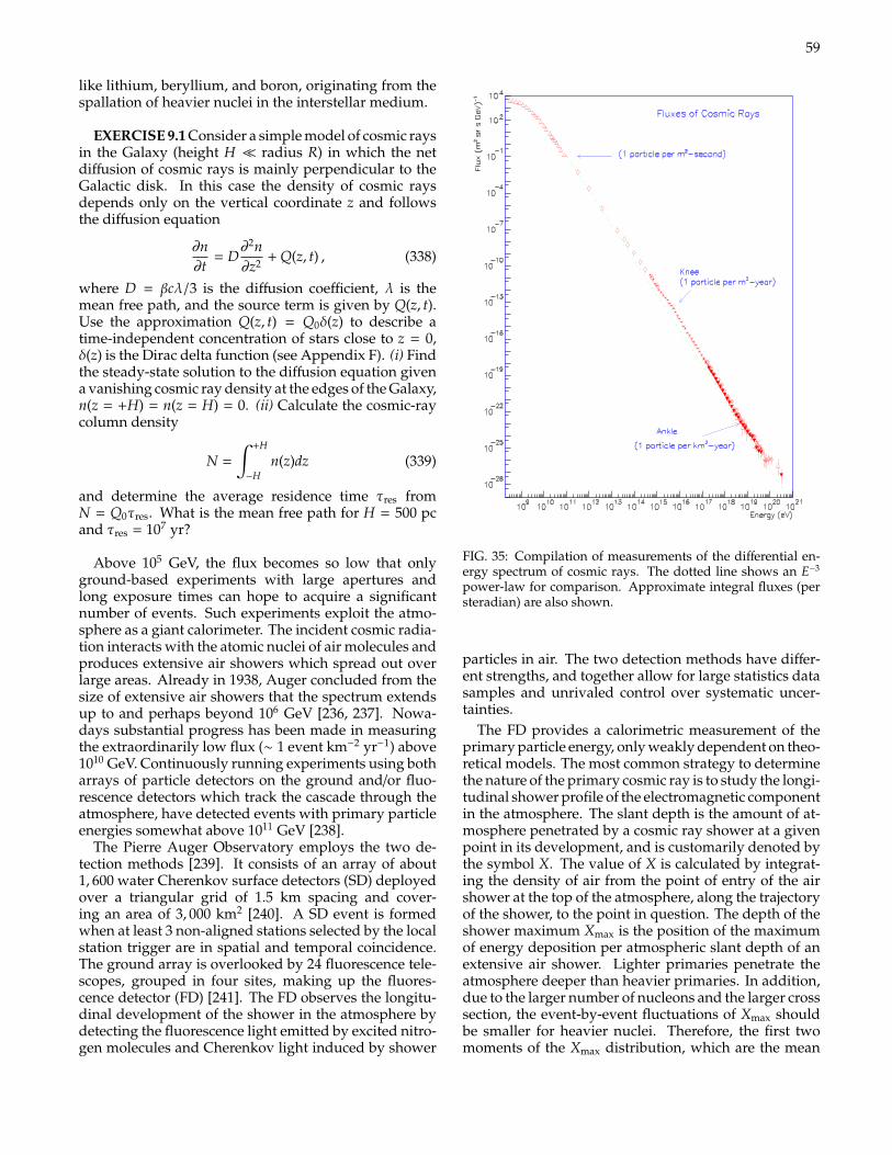
59

like lithium, beryllium, and boron, originating from thespallation of heavier nuclei in the interstellar medium.

EXERCISE 9.1 Consider a simple model of cosmic raysin the Galaxy (height H radius R) in which the netdiffusion of cosmic rays is mainly perpendicular to theGalactic disk. In this case the density of cosmic raysdepends only on the vertical coordinate z and followsthe diffusion equation

∂n∂t

= D∂2n∂z2 + Q(z, t) , (338)

where D = βcλ/3 is the diffusion coefficient, λ is themean free path, and the source term is given by Q(z, t).Use the approximation Q(z, t) = Q0δ(z) to describe atime-independent concentration of stars close to z = 0,δ(z) is the Dirac delta function (see Appendix F). (i) Findthe steady-state solution to the diffusion equation givena vanishing cosmic ray density at the edges of the Galaxy,n(z = +H) = n(z = H) = 0. (ii) Calculate the cosmic-raycolumn density

N =

∫ +H

−Hn(z)dz (339)

and determine the average residence time τres fromN = Q0τres. What is the mean free path for H = 500 pcand τres = 107 yr?

Above 105 GeV, the flux becomes so low that onlyground-based experiments with large apertures andlong exposure times can hope to acquire a significantnumber of events. Such experiments exploit the atmo-sphere as a giant calorimeter. The incident cosmic radia-tion interacts with the atomic nuclei of air molecules andproduces extensive air showers which spread out overlarge areas. Already in 1938, Auger concluded from thesize of extensive air showers that the spectrum extendsup to and perhaps beyond 106 GeV [236, 237]. Nowa-days substantial progress has been made in measuringthe extraordinarily low flux (∼ 1 event km−2 yr−1) above1010 GeV. Continuously running experiments using botharrays of particle detectors on the ground and/or fluo-rescence detectors which track the cascade through theatmosphere, have detected events with primary particleenergies somewhat above 1011 GeV [238].

The Pierre Auger Observatory employs the two de-tection methods [239]. It consists of an array of about1, 600 water Cherenkov surface detectors (SD) deployedover a triangular grid of 1.5 km spacing and cover-ing an area of 3, 000 km2 [240]. A SD event is formedwhen at least 3 non-aligned stations selected by the localstation trigger are in spatial and temporal coincidence.The ground array is overlooked by 24 fluorescence tele-scopes, grouped in four sites, making up the fluores-cence detector (FD) [241]. The FD observes the longitu-dinal development of the shower in the atmosphere bydetecting the fluorescence light emitted by excited nitro-gen molecules and Cherenkov light induced by shower

FIG. 35: Compilation of measurements of the differential en-ergy spectrum of cosmic rays. The dotted line shows an E−3

power-law for comparison. Approximate integral fluxes (persteradian) are also shown.

particles in air. The two detection methods have differ-ent strengths, and together allow for large statistics datasamples and unrivaled control over systematic uncer-tainties.

The FD provides a calorimetric measurement of theprimary particle energy, only weakly dependent on theo-retical models. The most common strategy to determinethe nature of the primary cosmic ray is to study the longi-tudinal shower profile of the electromagnetic componentin the atmosphere. The slant depth is the amount of at-mosphere penetrated by a cosmic ray shower at a givenpoint in its development, and is customarily denoted bythe symbol X. The value of X is calculated by integrat-ing the density of air from the point of entry of the airshower at the top of the atmosphere, along the trajectoryof the shower, to the point in question. The depth of theshower maximum Xmax is the position of the maximumof energy deposition per atmospheric slant depth of anextensive air shower. Lighter primaries penetrate theatmosphere deeper than heavier primaries. In addition,due to the larger number of nucleons and the larger crosssection, the event-by-event fluctuations of Xmax shouldbe smaller for heavier nuclei. Therefore, the first twomoments of the Xmax distribution, which are the mean

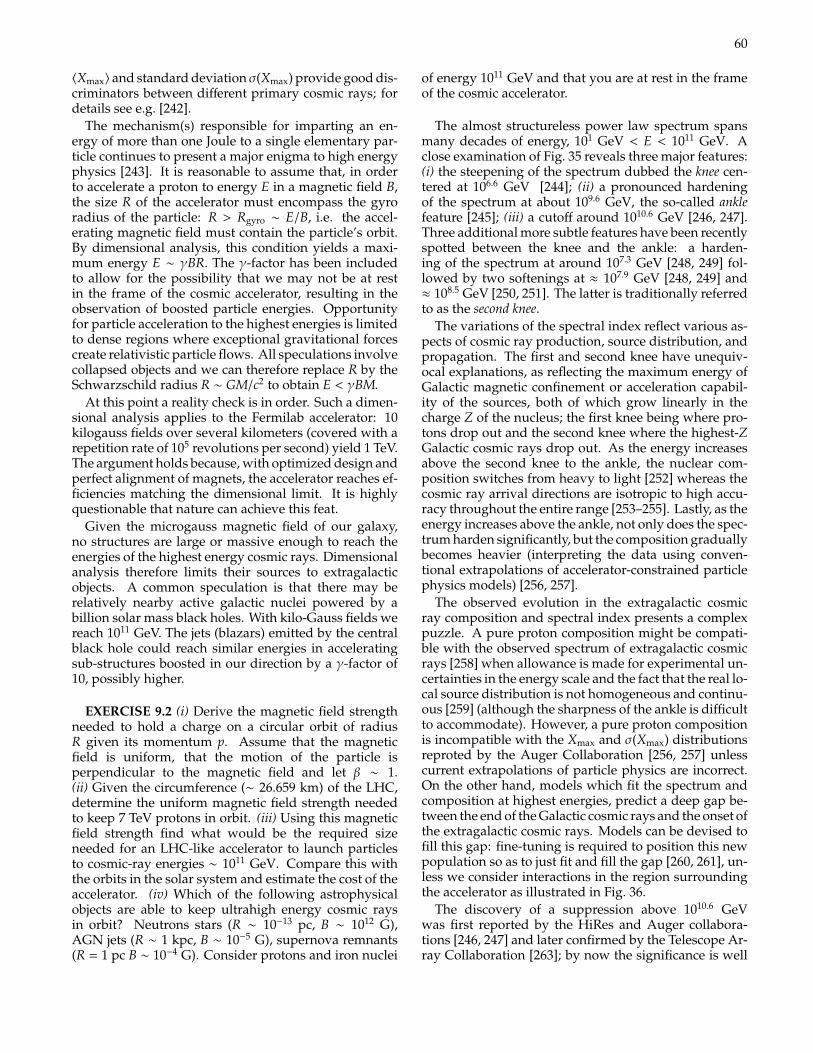
60

〈Xmax〉 and standard deviation σ(Xmax) provide good dis-criminators between different primary cosmic rays; fordetails see e.g. [242].

The mechanism(s) responsible for imparting an en-ergy of more than one Joule to a single elementary par-ticle continues to present a major enigma to high energyphysics [243]. It is reasonable to assume that, in orderto accelerate a proton to energy E in a magnetic field B,the size R of the accelerator must encompass the gyroradius of the particle: R > Rgyro ∼ E/B, i.e. the accel-erating magnetic field must contain the particle’s orbit.By dimensional analysis, this condition yields a maxi-mum energy E ∼ γBR. The γ-factor has been includedto allow for the possibility that we may not be at restin the frame of the cosmic accelerator, resulting in theobservation of boosted particle energies. Opportunityfor particle acceleration to the highest energies is limitedto dense regions where exceptional gravitational forcescreate relativistic particle flows. All speculations involvecollapsed objects and we can therefore replace R by theSchwarzschild radius R ∼ GM/c2 to obtain E < γBM.

At this point a reality check is in order. Such a dimen-sional analysis applies to the Fermilab accelerator: 10kilogauss fields over several kilometers (covered with arepetition rate of 105 revolutions per second) yield 1 TeV.The argument holds because, with optimized design andperfect alignment of magnets, the accelerator reaches ef-ficiencies matching the dimensional limit. It is highlyquestionable that nature can achieve this feat.

Given the microgauss magnetic field of our galaxy,no structures are large or massive enough to reach theenergies of the highest energy cosmic rays. Dimensionalanalysis therefore limits their sources to extragalacticobjects. A common speculation is that there may berelatively nearby active galactic nuclei powered by abillion solar mass black holes. With kilo-Gauss fields wereach 1011 GeV. The jets (blazars) emitted by the centralblack hole could reach similar energies in acceleratingsub-structures boosted in our direction by a γ-factor of10, possibly higher.

EXERCISE 9.2 (i) Derive the magnetic field strengthneeded to hold a charge on a circular orbit of radiusR given its momentum p. Assume that the magneticfield is uniform, that the motion of the particle isperpendicular to the magnetic field and let β ∼ 1.(ii) Given the circumference (∼ 26.659 km) of the LHC,determine the uniform magnetic field strength neededto keep 7 TeV protons in orbit. (iii) Using this magneticfield strength find what would be the required sizeneeded for an LHC-like accelerator to launch particlesto cosmic-ray energies ∼ 1011 GeV. Compare this withthe orbits in the solar system and estimate the cost of theaccelerator. (iv) Which of the following astrophysicalobjects are able to keep ultrahigh energy cosmic raysin orbit? Neutrons stars (R ∼ 10−13 pc, B ∼ 1012 G),AGN jets (R ∼ 1 kpc, B ∼ 10−5 G), supernova remnants(R = 1 pc B ∼ 10−4 G). Consider protons and iron nuclei

of energy 1011 GeV and that you are at rest in the frameof the cosmic accelerator.

The almost structureless power law spectrum spansmany decades of energy, 101 GeV < E < 1011 GeV. Aclose examination of Fig. 35 reveals three major features:(i) the steepening of the spectrum dubbed the knee cen-tered at 106.6 GeV [244]; (ii) a pronounced hardeningof the spectrum at about 109.6 GeV, the so-called anklefeature [245]; (iii) a cutoff around 1010.6 GeV [246, 247].Three additional more subtle features have been recentlyspotted between the knee and the ankle: a harden-ing of the spectrum at around 107.3 GeV [248, 249] fol-lowed by two softenings at ≈ 107.9 GeV [248, 249] and≈ 108.5 GeV [250, 251]. The latter is traditionally referredto as the second knee.

The variations of the spectral index reflect various as-pects of cosmic ray production, source distribution, andpropagation. The first and second knee have unequiv-ocal explanations, as reflecting the maximum energy ofGalactic magnetic confinement or acceleration capabil-ity of the sources, both of which grow linearly in thecharge Z of the nucleus; the first knee being where pro-tons drop out and the second knee where the highest-ZGalactic cosmic rays drop out. As the energy increasesabove the second knee to the ankle, the nuclear com-position switches from heavy to light [252] whereas thecosmic ray arrival directions are isotropic to high accu-racy throughout the entire range [253–255]. Lastly, as theenergy increases above the ankle, not only does the spec-trum harden significantly, but the composition graduallybecomes heavier (interpreting the data using conven-tional extrapolations of accelerator-constrained particlephysics models) [256, 257].

The observed evolution in the extragalactic cosmicray composition and spectral index presents a complexpuzzle. A pure proton composition might be compati-ble with the observed spectrum of extragalactic cosmicrays [258] when allowance is made for experimental un-certainties in the energy scale and the fact that the real lo-cal source distribution is not homogeneous and continu-ous [259] (although the sharpness of the ankle is difficultto accommodate). However, a pure proton compositionis incompatible with the Xmax and σ(Xmax) distributionsreproted by the Auger Collaboration [256, 257] unlesscurrent extrapolations of particle physics are incorrect.On the other hand, models which fit the spectrum andcomposition at highest energies, predict a deep gap be-tween the end of the Galactic cosmic rays and the onset ofthe extragalactic cosmic rays. Models can be devised tofill this gap: fine-tuning is required to position this newpopulation so as to just fit and fill the gap [260, 261], un-less we consider interactions in the region surroundingthe accelerator as illustrated in Fig. 36.

The discovery of a suppression above 1010.6 GeVwas first reported by the HiRes and Auger collabora-tions [246, 247] and later confirmed by the Telescope Ar-ray Collaboration [263]; by now the significance is well

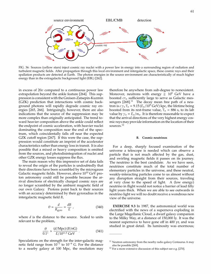
61

cosmic ray

source environment EBL/CMB detection

FIG. 36: Sources (yellow stars) inject cosmic ray nuclei with a power law in energy into a surrounding region of radiation andturbulent magnetic fields. After propagation through this local environment and intergalactic space, these cosmic rays and theirspallation products are detected at Earth. The photon energies in the source environment are characteristically of much higherenergy than in the extragalactic background light (EBL) [262].

in excess of 20σ compared to a continuous power lawextrapolation beyond the ankle feature [264]. This sup-pression is consistent with the Greisen-Zatsepin-Kuzmin(GZK) prediction that interactions with cosmic back-ground photons will rapidly degrade cosmic ray en-ergies [265, 266]. Intriguingly, however, there are alsoindications that the source of the suppression may bemore complex than originally anticipated. The trend to-ward heavier composition above the ankle could reflectthe endpoint of cosmic acceleration, with heavier nucleidominating the composition near the end of the spec-trum, which coincidentally falls off near the expectedGZK cutoff region [267]. If this were the case, the sup-pression would constitute an imprint of the acceleratorcharacteristics rather than energy loss in transit. It is alsopossible that a mixed or heavy composition is emittedfrom the sources, and photodisintegration of nuclei andother GZK energy losses suppress the flux.

The main reason why this impressive set of data failsto reveal the origin of the particles is undoubtedly thattheir directions have been scrambled by the microgaussGalactic magnetic fields. However, above 1010 GeV pro-ton astronomy could still be possible because the ar-rival directions of electrically charged cosmic rays areno longer scrambled by the ambient magnetic field ofour own Galaxy. Protons point back to their sourceswith an accuracy determined by their gyroradius in theintergalactic magnetic field B,

θ 'd

Rgyro=

dBE, (340)

where d is the distance to the source. Scaled to unitsrelevant to the problem,

θ0.1

'(d/Mpc) (B/nG)

E/1011.5 GeV. (341)

Speculations on the strength for the inter-galactic mag-netic field range from 10−7 to 10−9 G. For the distanceto a nearby galaxy at 100 Mpc, the resolution may

therefore be anywhere from sub-degree to nonexistent.Moreover, neutrons with energy & 109 GeV have aboosted cτn sufficiently large to serve as Galactic mes-sengers [268].11 The decay mean free path of a neu-tron is cγn τn = 9.15 (En/109 GeV) kpc, the lifetime beingboosted from its rest-frame value, τn = 886 s, to its labvalue by γn = En/mn. It is therefore reasonable to expectthat the arrival directions of the very highest energy cos-mic rays may provide information on the location of theirsources.12

B. Cosmic neutrinos

For a deep, sharply focused examination of theuniverse a telescope is needed which can observe aparticle that is not much affected by the gas, dust,and swirling magnetic fields it passes on its journey.The neutrino is the best candidate. As we have seen,neutrinos constitute much of the total number ofelementary particles in the universe, and these neutral,weakly-interacting particles come to us almost withoutany disruption straight from their sources, travelingat very close to the speed of light. A (low energy)neutrino in flight would not notice a barrier of lead fiftylight years thick. When we are able to see outwards inneutrino light we will no doubt receive a wondrous newview of the universe.

EXERCISE 9.3 In 1987, the astronomical world waselectrified with the news of a supernova exploding inthe Large Magellanic Cloud, a dwarf galaxy companionto the Milky Way, at a distance of 150,000 ly. It was thenearest supernova to have gone off in 400 yr, and wasstudied in great detail. Its luminosity was enormous;

11 Neutron astronomy from the nearby radio galaxy Centaurus A mayalso be possible [269].

12 For a more extensive discussion of this subject see e.g. [270].

62

the explosion released as much visible light energy ina few weeks as the Sun will emit in its entire lifetimeof 1010 yr. It was easily visible to the naked eye fromthe Southern hemisphere. However, models of themechanisms taking place in the supernovae predictthat the visible light represents only 1% of the totalenergy of the supernova; there is 100 times more energyemitted in the form of neutrinos, in a blast lasting onlya few seconds. (i) Calculate the total amount of energyemitted by the supernova in neutrinos. Express youranswer in Joules. (ii) Each neutrino has an energyof roughly 〈Eν〉 ∼ 1.5 × 10−12 J. Calculate how manyneutrinos are emitted by the supernova. (This is an easycalculation, but will give you a very large number).(iii) Kamiokande is one of the largest neutrino detectors.In 1987, it consisted of 2.140 kton of water (it hassince been expanded). Calculate how many electronneutrinos should have been detected by Kamiokande ifthe detection efficiency at 〈Eνe〉 ia bout 60% [271].

We have seen that MeV neutrinos are are produced bynuclear reaction chains in the central core of stars. Mov-ing up in energy, neutrinos would also be inevitablyproduced in many of the most luminous and energeticobjects in the universe. Whatever the source, the ma-chinery which accelerates cosmic rays will inevitablyalso produce neutrinos, guaranteeing that high energyneutrinos surely arrive to us from the cosmos.

Neutrino detectors must be generally placed deep un-derground, or in water, in order to escape the back-grounds caused by the inescapable rain of cosmic raysupon the atmosphere. These cosmic rays produce manymuons which penetrate deeply into the earth, in even thedeepest mines, but of course with ever-decreasing num-bers with depth. Hence the first attempts at high energyneutrino astronomy have been initiated underwater andunder ice [272].

The IceCube facility is located near the Amundsen-Scott station below the surface of the Antarctic ice sheetat the geographic South Pole [273]. The main part of thedetector is the InIce array, which covers a cubic kilometerof Antarctic glacial ice instrumented with digital opti-cal modules (DOMs) that detect Cherenkov ligh [274].The DOMs are attached to km-long supply and read-out cables called strings. Each string carries 60 DOMsspaced evenly along 1 km. The full baseline design of86 strings was completed in December 2010. In addi-tion to the InIce array, IceCube also possesses an airshower array called IceTop which comprises 80 stations,each of which consists of two tanks of water-ice instru-mented with 2 DOMs to detect Cherenkov light [275].The hybrid observations of air showers in the InIce andIceTop arrays have mutual benefits, namely significantair shower background rejection (for neutrino studies)and an improved air shower muon detection (for cosmicray studies).

In 2012, the IceCube Collaboration famously an-nounced an observation of two ∼ 1 PeV neutrinos dis-

covered in a search for the nearly guaranteed cosmo-genic neutrinos (which are expected to produced as sec-ondaries in the GZK chain reaction [276]) [277]. Thesearch technique was later refined to extend the neu-trino sensitivity to lower energies [278, 279], resultingin the discovery of an additional 26 neutrino candi-dates with energies between 50 TeV and 2 PeV, constitut-ing a 4.1σ excess for the combined 28 events comparedto expectations from neutrino and muon backgroundsgenerated in Earth’s atmosphere [280]. Interpretationof these results, however, does not appear to be en-tirely straightforward. For instance, if one makes thecommon assumption of an unbroken E−2

ν neutrino en-ergy spectrum, then one expects to observe about 8-9events with higher energies than the two highest energyevents observed thus far. The compatibility between Ice-Cube observations and the hypothesis of an unbrokenpower-law spectrum requires a rather steep spectrum,Φ(Eν) ∝ E−2.3 [281]. Very recently, the IceCube resultshave been updated [282–284]. At the time of writing, 54events have been reported in four years of IceCube datataking (1347 days between 2010 – 2014). The data are con-sistent with expectations for equal fluxes of all three neu-trino flavors [285]. The best-fit power law is E2

νΦ(Eν) =2.2±0.7×10−8(Eν/100 TeV)−0.58 GeV cm−2 s−1sr−1 and re-jects a purely atmospheric explanation at more than 5.7σ.Splitting the data into two sets, one from the northernsky and one from the souther sky, allows for a satisfac-tory power law fit with a different spectral index for eachhemisphere. The best-fit spectral index in the northernsky is γN = 2.0+0.3

−0.4, whereas in the southern sky it isγS = 2.56 ± 0.12 [283]. The discrepancy with respect toa single power law corresponds to 1.1σ and may indi-cate that the neutrino flux is anisotropic [286, 287]. Thelargest concentration of events is at or near the Galacticcenter, within uncertainties of their reconstructed arrivaldirections [288–290]. There are numerous proposed ex-planations for the origin of IceCubes events [291]. How-ever, considerably more data are yet required before thefinal verdict can be given.

C. Gravitational waves

Ever since Newton in the XVII century, we havelearned that gravity is a force that acts immediatelyon an object. In Einstein theory of general relativity,however, gravity is not a force at all, but a curvaturein space [61]. In other words, the presence of a verymassive body does not affect probed objects directly; itwarps the space around it first and then the objects movein the curved space. Inherit from such a redefinition ofgravity is the concept of gravitational waves: as mas-sive bodies move around, disturbances in the curvatureof spacetime can spread outward, much like a pebbletossed into a pond will cause waves to ripple outwardfrom the source. Propagating at (or near) the speed oflight, these disturbances do not travel through spacetime

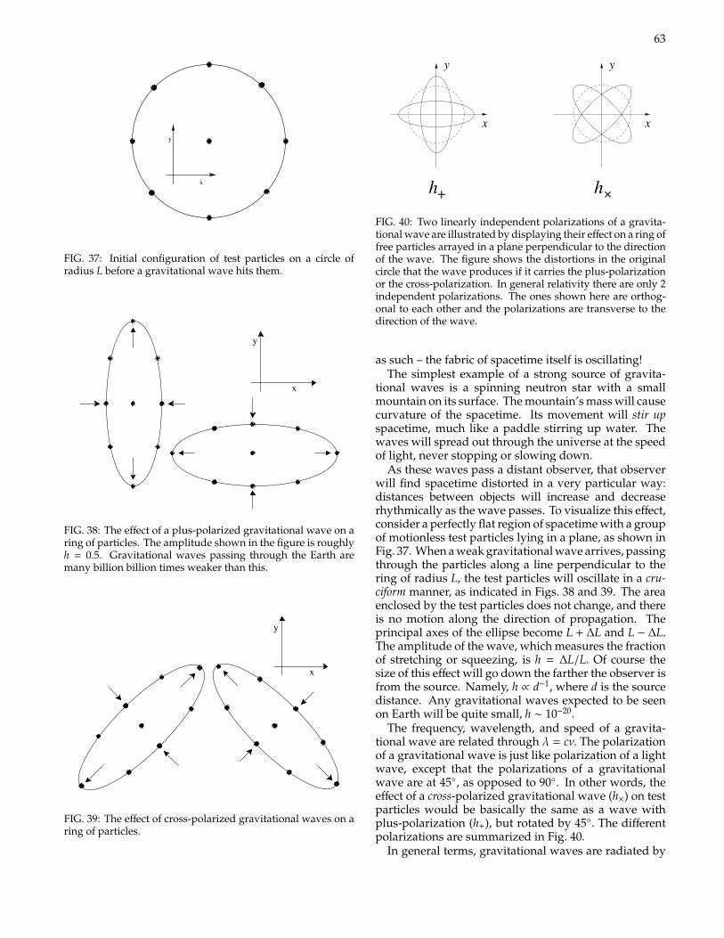
63

x

y

FIG. 37: Initial configuration of test particles on a circle ofradius L before a gravitational wave hits them.

y

x

FIG. 38: The effect of a plus-polarized gravitational wave on aring of particles. The amplitude shown in the figure is roughlyh = 0.5. Gravitational waves passing through the Earth aremany billion billion times weaker than this.

x

y

FIG. 39: The effect of cross-polarized gravitational waves on aring of particles.

y

x

y

x

h h+ +FIG. 40: Two linearly independent polarizations of a gravita-tional wave are illustrated by displaying their effect on a ring offree particles arrayed in a plane perpendicular to the directionof the wave. The figure shows the distortions in the originalcircle that the wave produces if it carries the plus-polarizationor the cross-polarization. In general relativity there are only 2independent polarizations. The ones shown here are orthog-onal to each other and the polarizations are transverse to thedirection of the wave.

as such – the fabric of spacetime itself is oscillating!The simplest example of a strong source of gravita-

tional waves is a spinning neutron star with a smallmountain on its surface. The mountain’s mass will causecurvature of the spacetime. Its movement will stir upspacetime, much like a paddle stirring up water. Thewaves will spread out through the universe at the speedof light, never stopping or slowing down.

As these waves pass a distant observer, that observerwill find spacetime distorted in a very particular way:distances between objects will increase and decreaserhythmically as the wave passes. To visualize this effect,consider a perfectly flat region of spacetime with a groupof motionless test particles lying in a plane, as shown inFig. 37. When a weak gravitational wave arrives, passingthrough the particles along a line perpendicular to thering of radius L, the test particles will oscillate in a cru-ciform manner, as indicated in Figs. 38 and 39. The areaenclosed by the test particles does not change, and thereis no motion along the direction of propagation. Theprincipal axes of the ellipse become L + ∆L and L − ∆L.The amplitude of the wave, which measures the fractionof stretching or squeezing, is h = ∆L/L. Of course thesize of this effect will go down the farther the observer isfrom the source. Namely, h ∝ d−1, where d is the sourcedistance. Any gravitational waves expected to be seenon Earth will be quite small, h ∼ 10−20.

The frequency, wavelength, and speed of a gravita-tional wave are related through λ = cν. The polarizationof a gravitational wave is just like polarization of a lightwave, except that the polarizations of a gravitationalwave are at 45, as opposed to 90. In other words, theeffect of a cross-polarized gravitational wave (h×) on testparticles would be basically the same as a wave withplus-polarization (h+), but rotated by 45. The differentpolarizations are summarized in Fig. 40.

In general terms, gravitational waves are radiated by

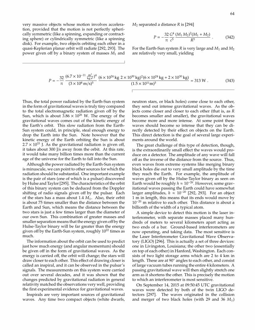
64

very massive objects whose motion involves accelera-tion, provided that the motion is not perfectly spheri-cally symmetric (like a spinning, expanding or contract-ing sphere) or cylindrically symmetric (like a spinningdisk). For example, two objects orbiting each other in aquasi-Keplerian planar orbit will radiate [292, 293]. Thepower given off by a binary system of masses M1 and

M2 separated a distance R is [294]

P = −32π

G4

c5

(M1 M2)2(M1 + M2)R5 . (342)

For the Earth-Sun system R is very large and M1 and M2are relatively very small, yielding

P = −32π

(6.7 × 10−11 m3

kg s2 )4

(3 × 108 m/s)5

(6 × 1024 kg 2 × 1030 kg)2(6 × 1024 kg + 2 × 1030 kg)(1.5 × 1011m)5 = 313 W . (343)

Thus, the total power radiated by the Earth-Sun systemin the form of gravitational waves is truly tiny comparedto the total electromagnetic radiation given off by theSun, which is about 3.86 × 1026 W. The energy of thegravitational waves comes out of the kinetic energy ofthe Earth’s orbit. This slow radiation from the Earth-Sun system could, in principle, steal enough energy todrop the Earth into the Sun. Note however that thekinetic energy of the Earth orbiting the Sun is about2.7 × 1033 J. As the gravitational radiation is given off,it takes about 300 J/s away from the orbit. At this rate,it would take many billion times more than the currentage of the universe for the Earth to fall into the Sun.

Although the power radiated by the Earth-Sun systemis minuscule, we can point to other sources for which theradiation should be substantial. One important exampleis the pair of stars (one of which is a pulsar) discoveredby Hulse and Taylor [295]. The characteristics of the orbitof this binary system can be deduced from the Dopplershifting of radio signals given off by the pulsar. Eachof the stars has a mass about 1.4 M. Also, their orbitis about 75 times smaller than the distance between theEarth and Sun, which means the distance between thetwo stars is just a few times larger than the diameter ofour own Sun. This combination of greater masses andsmaller separation means that the energy given off by theHulse-Taylor binary will be far greater than the energygiven off by the Earth-Sun system, roughly 1022 times asmuch.

The information about the orbit can be used to predictjust how much energy (and angular momentum) shouldbe given off in the form of gravitational waves. As theenergy is carried off, the orbit will change; the stars willdraw closer to each other. This effect of drawing closer iscalled an inspiral, and it can be observed in the pulsar’ssignals. The measurements on this system were carriedout over several decades, and it was shown that thechanges predicted by gravitational radiation in generalrelativity matched the observations very well, providingthe first experimental evidence for gravitational waves.

Inspirals are very important sources of gravitationalwaves. Any time two compact objects (white dwarfs,

neutron stars, or black holes) come close to each other,they send out intense gravitational waves. As the ob-jects come closer and closer to each other (that is, as Rbecomes smaller and smaller), the gravitational wavesbecome more and more intense. At some point thesewaves should become so intense that they can be di-rectly detected by their effect on objects on the Earth.This direct detection is the goal of several large experi-ments around the world.

The great challenge of this type of detection, though,is the extraordinarily small effect the waves would pro-duce on a detector. The amplitude of any wave will falloff as the inverse of the distance from the source. Thus,even waves from extreme systems like merging binaryblack holes die out to very small amplitude by the timethey reach the Earth. For example, the amplitude ofwaves given off by the Hulse-Taylor binary as seen onEarth would be roughly h ≈ 10−26.However, some grav-itational waves passing the Earth could have somewhatlarger amplitudes, h ≈ 10−20 [292, 293]. For an object1 m in length, this means that its ends would move by10−20 m relative to each other. This distance is about abillionth of the width of a typical atom.

A simple device to detect this motion is the laser in-terferometer, with separate masses placed many hun-dreds of meters to several kilometers apart acting astwo ends of a bar. Ground-based interferometers arenow operating, and taking data. The most sensitive isthe Laser Interferometer Gravitational Wave Observa-tory (LIGO) [296]. This is actually a set of three devices:one in Livingston, Louisiana; the other two (essentiallyon top of each other) in Hanford, Washington. Each con-sists of two light storage arms which are 2 to 4 km inlength. These are at 90 angles to each other, and consistof large vacuum tubes running the entire 4 kilometers. Apassing gravitational wave will then slightly stretch onearm as it shortens the other. This is precisely the motionto which an interferometer is most sensitive.

On September 14, 2015 at 09:50:45 UTC gravitationalwaves were detected by both of the twin LIGO de-tectors [297]. The waves originated in the collisionand merger of two black holes (with 29 and 36 M)

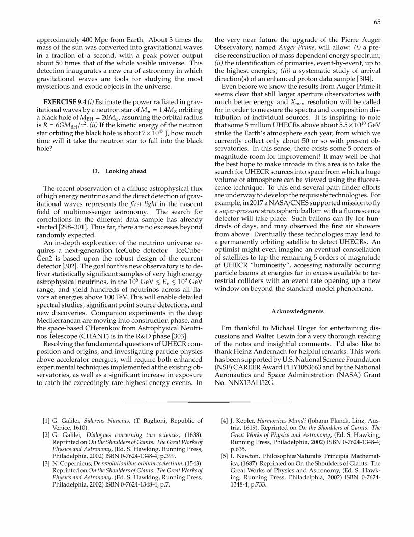
65

approximately 400 Mpc from Earth. About 3 times themass of the sun was converted into gravitational wavesin a fraction of a second, with a peak power outputabout 50 times that of the whole visible universe. Thisdetection inaugurates a new era of astronomy in whichgravitational waves are tools for studying the mostmysterious and exotic objects in the universe.

EXERCISE 9.4 (i) Estimate the power radiated in grav-itational waves by a neutron star of M? = 1.4M orbitinga black hole of MBH = 20M, assuming the orbital radiusis R = 6GMBH/c2. (ii) If the kinetic energy of the neutronstar orbiting the black hole is about 7× 1047 J, how muchtime will it take the neutron star to fall into the blackhole?

D. Looking ahead

The recent observation of a diffuse astrophysical fluxof high energy neutrinos and the direct detection of grav-itational waves represents the first light in the nascentfield of multimessenger astronomy. The search forcorrelations in the different data sample has alreadystarted [298–301]. Thus far, there are no excesses beyondrandomly expected.

An in-depth exploration of the neutrino universe re-quires a next-generation IceCube detector. IceCube-Gen2 is based upon the robust design of the currentdetector [302]. The goal for this new observatory is to de-liver statistically significant samples of very high energyastrophysical neutrinos, in the 106 GeV . Eν . 109 GeVrange, and yield hundreds of neutrinos across all fla-vors at energies above 100 TeV. This will enable detailedspectral studies, significant point source detections, andnew discoveries. Companion experiments in the deepMediterranean are moving into construction phase, andthe space-based CHerenkov from Astrophysical Neutri-nos Telescope (CHANT) is in the R&D phase [303].

Resolving the fundamental questions of UHECR com-position and origins, and investigating particle physicsabove accelerator energies, will require both enhancedexperimental techniques implemented at the existing ob-servatories, as well as a significant increase in exposureto catch the exceedingly rare highest energy events. In

the very near future the upgrade of the Pierre AugerObservatory, named Auger Prime, will allow: (i) a pre-cise reconstruction of mass dependent energy spectrum;(ii) the identification of primaries, event-by-event, up tothe highest energies; (iii) a systematic study of arrivaldirection(s) of an enhanced proton data sample [304].

Even before we know the results from Auger Prime itseems clear that still larger aperture observatories withmuch better energy and Xmax resolution will be calledfor in order to measure the spectra and composition dis-tribution of individual sources. It is inspiring to notethat some 5 million UHECRs above about 5.5×1010 GeVstrike the Earth’s atmosphere each year, from which wecurrently collect only about 50 or so with present ob-servatories. In this sense, there exists some 5 orders ofmagnitude room for improvement! It may well be thatthe best hope to make inroads in this area is to take thesearch for UHECR sources into space from which a hugevolume of atmosphere can be viewed using the fluores-cence technique. To this end several path finder effortsare underway to develop the requisiste technologies. Forexample, in 2017 a NASA/CNES supported mission to flya super-pressure stratospheric ballom with a fluorescencedetector will take place. Such ballons can fly for hun-dreds of days, and may observed the first air showersfrom above. Eventually these technologies may lead toa permanently orbiting satellite to detect UHECRs. Anoptimist might even imagine an eventual constellationof satellites to tap the remaining 5 orders of magnitudeof UHECR “luminosity”, accessing naturally occuringparticle beams at energies far in excess available to ter-restrial colliders with an event rate opening up a newwindow on beyond-the-standard-model phenomena.

Acknowledgments

I’m thankful to Michael Unger for entertaining dis-cussions and Walter Lewin for a very thorough readingof the notes and insightful comments. I’d also like tothank Heinz Andernach for helpful remarks. This workhas been supported by U.S. National Science Foundation(NSF) CAREER Award PHY1053663 and by the NationalAeronautics and Space Administration (NASA) GrantNo. NNX13AH52G.

[1] G. Galilei, Sidereus Nuncius, (T. Baglioni, Republic ofVenice, 1610).

[2] G. Galilei, Dialogues concerning two sciences, (1638).Reprinted on On the Shoulders of Giants: The Great Works ofPhysics and Astronomy, (Ed. S. Hawking, Running Press,Philadelphia, 2002) ISBN 0-7624-1348-4; p.399.

[3] N. Copernicus, De revolutionibus orbium coelestium, (1543).Reprinted on On the Shoulders of Giants: The Great Works ofPhysics and Astronomy, (Ed. S. Hawking, Running Press,Philadelphia, 2002) ISBN 0-7624-1348-4; p.7.

[4] J. Kepler, Harmonices Mundi (Johann Planck, Linz, Aus-tria, 1619). Reprinted on On the Shoulders of Giants: TheGreat Works of Physics and Astronomy, (Ed. S. Hawking,Running Press, Philadelphia, 2002) ISBN 0-7624-1348-4;p.635.

[5] I. Newton, PhilosophiæNaturalis Principia Mathemat-ica, (1687). Reprinted on On the Shoulders of Giants: TheGreat Works of Physics and Astronomy, (Ed. S. Hawk-ing, Running Press, Philadelphia, 2002) ISBN 0-7624-1348-4; p.733.

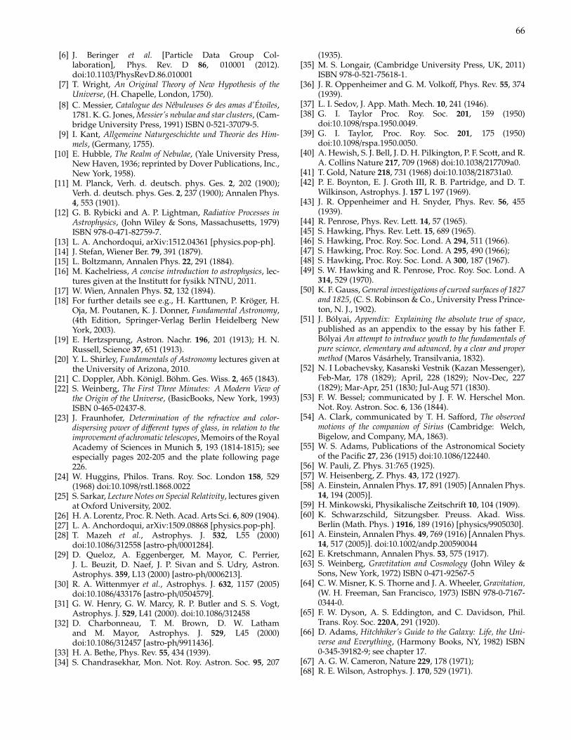
66

[6] J. Beringer et al. [Particle Data Group Col-laboration], Phys. Rev. D 86, 010001 (2012).doi:10.1103/PhysRevD.86.010001

[7] T. Wright, An Original Theory of New Hypothesis of theUniverse, (H. Chapelle, London, 1750).

[8] C. Messier, Catalogue des Nebuleuses & des amas d’Etoiles,1781. K. G. Jones, Messier’s nebulae and star clusters, (Cam-bridge University Press, 1991) ISBN 0-521-37079-5.

[9] I. Kant, Allgemeine Naturgeschichte und Theorie des Him-mels, (Germany, 1755).

[10] E. Hubble, The Realm of Nebulae, (Yale University Press,New Haven, 1936; reprinted by Dover Publications, Inc.,New York, 1958).

[11] M. Planck, Verh. d. deutsch. phys. Ges. 2, 202 (1900);Verh. d. deutsch. phys. Ges. 2, 237 (1900); Annalen Phys.4, 553 (1901).

[12] G. B. Rybicki and A. P. Lightman, Radiative Processes inAstrophysics, (John Wiley & Sons, Massachusetts, 1979)ISBN 978-0-471-82759-7.

[13] L. A. Anchordoqui, arXiv:1512.04361 [physics.pop-ph].[14] J. Stefan, Wiener Ber. 79, 391 (1879).[15] L. Boltzmann, Annalen Phys. 22, 291 (1884).[16] M. Kachelriess, A concise introduction to astrophysics, lec-

tures given at the Institutt for fysikk NTNU, 2011.[17] W. Wien, Annalen Phys. 52, 132 (1894).[18] For further details see e.g., H. Karttunen, P. Kroger, H.

Oja, M. Poutanen, K. J. Donner, Fundamental Astronomy,(4th Edition, Springer-Verlag Berlin Heidelberg NewYork, 2003).

[19] E. Hertzsprung, Astron. Nachr. 196, 201 (1913); H. N.Russell, Science 37, 651 (1913).

[20] Y. L. Shirley, Fundamentals of Astronomy lectures given atthe University of Arizona, 2010.

[21] C. Doppler, Abh. Konigl. Bohm. Ges. Wiss. 2, 465 (1843).[22] S. Weinberg, The First Three Minutes: A Modern View of

the Origin of the Universe, (BasicBooks, New York, 1993)ISBN 0-465-02437-8.

[23] J. Fraunhofer, Determination of the refractive and color-dispersing power of different types of glass, in relation to theimprovement of achromatic telescopes, Memoirs of the RoyalAcademy of Sciences in Munich 5, 193 (1814-1815); seeespecially pages 202-205 and the plate following page226.

[24] W. Huggins, Philos. Trans. Roy. Soc. London 158, 529(1968) doi:10.1098/rstl.1868.0022

[25] S. Sarkar, Lecture Notes on Special Relativity, lectures givenat Oxford University, 2002.

[26] H. A. Lorentz, Proc. R. Neth. Acad. Arts Sci. 6, 809 (1904).[27] L. A. Anchordoqui, arXiv:1509.08868 [physics.pop-ph].[28] T. Mazeh et al., Astrophys. J. 532, L55 (2000)

doi:10.1086/312558 [astro-ph/0001284].[29] D. Queloz, A. Eggenberger, M. Mayor, C. Perrier,

J. L. Beuzit, D. Naef, J. P. Sivan and S. Udry, Astron.Astrophys. 359, L13 (2000) [astro-ph/0006213].

[30] R. A. Wittenmyer et al., Astrophys. J. 632, 1157 (2005)doi:10.1086/433176 [astro-ph/0504579].

[31] G. W. Henry, G. W. Marcy, R. P. Butler and S. S. Vogt,Astrophys. J. 529, L41 (2000). doi:10.1086/312458

[32] D. Charbonneau, T. M. Brown, D. W. Lathamand M. Mayor, Astrophys. J. 529, L45 (2000)doi:10.1086/312457 [astro-ph/9911436].

[33] H. A. Bethe, Phys. Rev. 55, 434 (1939).[34] S. Chandrasekhar, Mon. Not. Roy. Astron. Soc. 95, 207

(1935).[35] M. S. Longair, (Cambridge University Press, UK, 2011)

ISBN 978-0-521-75618-1.[36] J. R. Oppenheimer and G. M. Volkoff, Phys. Rev. 55, 374

(1939).[37] L. I. Sedov, J. App. Math. Mech. 10, 241 (1946).[38] G. I. Taylor Proc. Roy. Soc. 201, 159 (1950)

doi:10.1098/rspa.1950.0049.[39] G. I. Taylor, Proc. Roy. Soc. 201, 175 (1950)

doi:10.1098/rspa.1950.0050.[40] A. Hewish, S. J. Bell, J. D. H. Pilkington, P. F. Scott, and R.

A. Collins Nature 217, 709 (1968) doi:10.1038/217709a0.[41] T. Gold, Nature 218, 731 (1968) doi:10.1038/218731a0.[42] P. E. Boynton, E. J. Groth III, R. B. Partridge, and D. T.

Wilkinson, Astrophys. J. 157 L 197 (1969).[43] J. R. Oppenheimer and H. Snyder, Phys. Rev. 56, 455

(1939).[44] R. Penrose, Phys. Rev. Lett. 14, 57 (1965).[45] S. Hawking, Phys. Rev. Lett. 15, 689 (1965).[46] S. Hawking, Proc. Roy. Soc. Lond. A 294, 511 (1966).[47] S. Hawking, Proc. Roy. Soc. Lond. A 295, 490 (1966);[48] S. Hawking, Proc. Roy. Soc. Lond. A 300, 187 (1967).[49] S. W. Hawking and R. Penrose, Proc. Roy. Soc. Lond. A

314, 529 (1970).[50] K. F. Gauss, General investigations of curved surfaces of 1827

and 1825, (C. S. Robinson & Co., University Press Prince-ton, N. J., 1902).

[51] J. Bolyai, Appendix: Explaining the absolute true of space,published as an appendix to the essay by his father F.Bolyai An attempt to introduce youth to the fundamentals ofpure science, elementary and advanced, by a clear and propermethod (Maros Vasarhely, Transilvania, 1832).

[52] N. I Lobachevsky, Kasanski Vestnik (Kazan Messenger),Feb-Mar, 178 (1829); April, 228 (1829); Nov-Dec, 227(1829); Mar-Apr, 251 (1830; Jul-Aug 571 (1830).

[53] F. W. Bessel; communicated by J. F. W. Herschel Mon.Not. Roy. Astron. Soc. 6, 136 (1844).

[54] A. Clark, communicated by T. H. Safford, The observedmotions of the companion of Sirius (Cambridge: Welch,Bigelow, and Company, MA, 1863).

[55] W. S. Adams, Publications of the Astronomical Societyof the Pacific 27, 236 (1915) doi:10.1086/122440.

[56] W. Pauli, Z. Phys. 31:765 (1925).[57] W. Heisenberg, Z. Phys. 43, 172 (1927).[58] A. Einstein, Annalen Phys. 17, 891 (1905) [Annalen Phys.

14, 194 (2005)].[59] H. Minkowski, Physikalische Zeitschrift 10, 104 (1909).[60] K. Schwarzschild, Sitzungsber. Preuss. Akad. Wiss.

Berlin (Math. Phys. ) 1916, 189 (1916) [physics/9905030].[61] A. Einstein, Annalen Phys. 49, 769 (1916) [Annalen Phys.

14, 517 (2005)]. doi:10.1002/andp.200590044[62] E. Kretschmann, Annalen Phys. 53, 575 (1917).[63] S. Weinberg, Gravtitation and Cosmology (John Wiley &

Sons, New York, 1972) ISBN 0-471-92567-5[64] C. W. Misner, K. S. Thorne and J. A. Wheeler, Gravitation,

(W. H. Freeman, San Francisco, 1973) ISBN 978-0-7167-0344-0.

[65] F. W. Dyson, A. S. Eddington, and C. Davidson, Phil.Trans. Roy. Soc. 220A, 291 (1920).

[66] D. Adams, Hitchhiker’s Guide to the Galaxy: Life, the Uni-verse and Everything, (Harmony Books, NY, 1982) ISBN0-345-39182-9; see chapter 17.

[67] A. G. W. Cameron, Nature 229, 178 (1971);[68] R. E. Wilson, Astrophys. J. 170, 529 (1971).

67

[69] R. Giacconi, P. Gorenstein, H. Gursky, J. R Waters, Astro-phys. J. 148, L119 (1967)

[70] M. Oda, P. Gorenstein, H. Gursky, E. Kellogg, E. Schreier,H. Tananbaum, R. Giacconi, Astrophys. J. 166, L1 (1971).

[71] B. L. Webster and P. Murdin, Nature, 235, 37 (1972).[72] C. T. Bolton, Nature 235, 271 (1972).[73] J. A. Petterson, Astrophys. J. 224, 625 (1978).[74] A. M. Stirling, R. E. Spencer, C. de la Force, M. A. Garrett,

R. P. Fender and R. N. Ogley, Mon. Not. Roy. Astron.Soc. 327, 1273 (2001) doi:10.1046/j.1365-8711.2001.04821.x[astro-ph/0107192].

[75] J. J. Thomson, Conduction of electricity through gases (Cam-bridge University Press, Cambridge, 1906).

[76] A. S. Eddington, The internal constitution of the stars (Cam-bridge University Press, Cambridge, 1926).

[77] J. Biteau, PhD thesis, 2013, pastel-00822242.[78] C. M. Urry and P. Padovani, Publ. Astron. Soc. Pac. 107,

803 (1995) doi:10.1086/133630 [astro-ph/9506063].[79] C. D. Dermer and B. Giebels, arXiv:1602.06592 [astro-

ph.HE].[80] B. G. Piner, D. Bhattarai, P. G. Edwards and D. L. Jones,

Astrophys. J. 640, 196 (2006) doi:10.1086/500006 [astro-ph/0511664].

[81] J. P. L. de Cheseaux, Traite de la Comete (Lausanne, 1774),pp. 223 ff; reprinted in The Bowl of Night, by F. P. Dickson(MIT Press, Cambridge, 1968) Appendix II.

[82] H. W. M. Olbers, Bode’s Jahrbuch, 111 (1826); reprinted byDickson, op. cit., Appendix I.

[83] E. Hubble, Proc. Nat. Acad. Sci. 15, 168 (1929).[84] W. L. Freedman et al. [HST Collaboration], Astrophys. J.

553, 47 (2001) doi:10.1086/320638 [astro-ph/0012376].[85] http://www.sdss.org/iotw/archive.html[86] C. F. Chyba, J. R. Gott, and A. Spitkovsky, The Universe,

lectures given at Princeton University, 2009 - 2010.[87] E. A. Milne, Z. Astrophysik 6, 1 (1933).[88] B. Ryden, Introduction to cosmology, (Addison-Wesley, San

Francisco, USA, 2003) ISBN 978-0805389128[89] A. Einstein, Sitzungsber. Preuss. Akad. Wiss. Berlin

(Math. Phys. ) 1917, 142 (1917).[90] A. Friedmann, Z. Phys. 10, 377 (1922).[91] A. Friedmann, Z. Phys. 21, 326 (1924).[92] H. P. Robertson, Astrophys. J. 82, 284 (1935).[93] H. P. Robertson, Astrophys. J. 83, 187, 257 (1936).[94] A. G. Walker, Proc. Lond. Math. Soc. (2), 42 90 (1936).[95] V. Mukhanov, Physical Foundations of Cosmology, (Cam-

bridge University Press, UK, 2005) ISBN: 978-0-521-56398-7

[96] N. Pogson, Mon. Not. Roy. Astron. Soc. 17, 12 (1856).[97] A. G. Riess et al. [Supernova Search Team Collaboration],

Astron. J. 116, 1009 (1998) doi:10.1086/300499 [astro-ph/9805201].

[98] S. Perlmutter et al. [Supernova Cosmology Project Collab-oration], Astrophys. J. 517, 565 (1999) doi:10.1086/307221[astro-ph/9812133].

[99] M. Hamuy et al, Astron. J. 106, 2392 (1993).[100] M. Hamuy, M. M. Phillips, J. Maza, N. B. Suntzeff,

R. A. Schommer and R. Aviles, Astron. J. 109, 1 (1995).doi:10.1086/117251

[101] S. Perlmutter, Phys. Today, April 2003.[102] N. A. Bahcall, J. P. Ostriker, S. Perlmutter

and P. J. Steinhardt, Science 284, 1481 (1999)doi:10.1126/science.284.5419.1481 [astro-ph/9906463].

[103] A. A. Penzias and R. W. Wilson, Astrophys. J. 142, 419(1965).

[104] R. H. Dicke, P. J. E. Peebles, P. G. Roll and D. T. Wilkinson,Astrophys. J. 142, 414 (1965). doi:10.1086/148306

[105] G. F. Smoot, astro-ph/9705101.[106] J. C. Mather et al., Astrophys. J. 420, 439 (1994).[107] C. L. Bennett et al. [WMAP Collaboration], Astrophys. J.

Suppl. 208, 20 (2013) [arXiv:1212.5225 [astro-ph.CO]].[108] R. Adam et al. [Planck Collaboration], arXiv:1502.01582

[astro-ph.CO].[109] S. Weinberg, Cosmology, (Oxford University Press, UK,

2008) ISBN 978-0-19-852682-7.[110] S. Dodelson, Modern Cosmology, (Academic Press, Else-

vier, Amsterdam, 2003) ISBN 978-0-12-219141-1.[111] L. A. Anchordoqui and T. C. Paul, Mathematical models

of physics problems (Nova, New York, 2013) ISBN 978-1-62618-600-2.

[112] P. B. Denton, L. A. Anchordoqui, A. A. Berlind,M. Richardson, and T. J. Weiler (for the JEM-EUSOCollaboration), J. Phys. Conf. Ser. 531, 012004 (2014)doi:10.1088/1742-6596/531/1/012004 [arXiv:1401.5757[astro-ph.IM]].

[113] G. Hinshaw et al. [WMAP Collaboration], Astrophys.J. Suppl. 180, 225 (2009) doi:10.1088/0067-0049/180/2/225[arXiv:0803.0732 [astro-ph]].

[114] C. H. Lineweaver, ASP Conf. Ser. 126, 185 (1997) [astro-ph/9702042].

[115] V. C. Rubin and W. K. Ford, Jr., Astrophys. J. 159, 379(1970). doi:10.1086/150317

[116] V. C. Rubin, N. Thonnard and W. K. Ford, Jr., Astrophys.J. 238, 471 (1980). doi:10.1086/158003

[117] V. C. Rubin, D. Burstein, W. K. Ford, Jr. and N. Thonnard,Astrophys. J. 289, 81 (1985). doi:10.1086/162866

[118] F. Zwicky, Helv. Phys. Acta 6, 110 (1933).[119] D. Clowe, M. Bradac, A. H. Gonzalez, M. Markevitch,

S. W. Randall, C. Jones and D. Zaritsky, Astrophys. J.648, L109 (2006) doi:10.1086/508162 [astro-ph/0608407].

[120] J. L. Feng, Ann. Rev. Astron. Astrophys. 48, 495(2010) doi:10.1146/annurev-astro-082708-101659[arXiv:1003.0904 [astro-ph.CO]].

[121] P. A. R. Ade et al. [Planck Collaboration],arXiv:1502.01589 [astro-ph.CO].

[122] A. G. Riess et al., Astrophys. J. 730, 119 (2011) Erratum:[Astrophys. J. 732, 129 (2011)] doi:10.1088/0004-637X/732/2/129, 10.1088/0004-637X/730/2/119[arXiv:1103.2976 [astro-ph.CO]].

[123] R. A. Knop et al. [Supernova Cosmology Project Col-laboration], Astrophys. J. 598, 102 (2003) [arXiv:astro-ph/0309368].

[124] S. W. Allen, R. W. Schmidt and A. C. Fabian, Mon.Not. Roy. Astron. Soc. 334, L11 (2002) [arXiv:astro-ph/0205007].

[125] A. E. Lange et al. [Boomerang Collaboration], Phys. Rev.D 63, 042001 (2001) [arXiv:astro-ph/0005004].

[126] A. Balbi et al., Astrophys. J. 545, L1 (2000) [Erratum-ibid.558, L145 (2001)] [arXiv:astro-ph/0005124].

[127] S. M. Carroll, W. H. Press and E. L. Turner, Ann. Rev.Astron. Astrophys. 30, 499 (1992).

[128] B. S. Meyer and D. N. Schramm, Astrophys. J. 311, 406(1986).

[129] G. Aldering et al. [SNAP Collaboration], arXiv:astro-ph/0209550.

[130] F. Halzen and A. D. Martin, Quarks and leptons: An in-troductory course In modern particle physics, (John Wiley &Sons, New York, 1984) ISBN 0-471-88741-2

[131] V. D. Barger and R. J. N. Phillips, Collider physics, Front.

68

Phys. 71, 1 (1991) ISBN 0-201-14945-1[132] C. Quigg, Gauge Theories of the strong, weak, and electro-

magnetic interactions, Front. Phys. 56, 1 (1983) ISBN 978-0805360202

[133] L. Anchordoqui and F. Halzen, arXiv:0906.1271[physics.ed-ph].

[134] K. A. Olive et al. [Particle Data Group Collabora-tion], Chin. Phys. C 38, 090001 (2014). doi:10.1088/1674-1137/38/9/090001

[135] H. Fritzsch, M. Gell-Mann and H. Leutwyler, Phys. Lett.B 47, 365 (1973).

[136] M. Gell-Mann, CTSL-20, TID-12608.[137] Y. Ne’eman, Nucl. Phys. 26, 222 (1961).[138] M. Gell-Mann, Phys. Lett. 8, 214 (1964).[139] S. N. Bose, Z. Phys. 26, 178 (1924).[140] A. Einstein, [Sitzungsber. Preuss. Akad. Wiss. Berlin

(Math. Phys. ) 22, 261 (1924); 1, 3 (1925); 3, 18 (1925).[141] E. Fermi, Rend. Lincei 3, 145 (1926); Z. Phys. 36, 902

(1926).[142] P. A. M. Dirac, Proc. R. Soc. Lond. Ser. A 112, 661 (1926).[143] D. J. Gross and F. Wilczek, Phys. Rev. Lett. 30, 1343 (1973).[144] H. D. Politzer, Phys. Rev. Lett. 30, 1346 (1973).[145] J. S. Schwinger, Phys. Rev. 74, 1439 (1948).[146] J. S. Schwinger, Phys. Rev. 75, 651 (1948).

doi:10.1103/PhysRev.75.651[147] S. Tomonaga, Prog. Theor. Phys. 1, 27 (1946).[148] R. P. Feynman, Rev. Mod. Phys. 20, 367 (1948).[149] F. J. Dyson, Phys. Rev. 75, 486 (1949).[150] F. J. Dyson, Phys. Rev. 75, 1736 (1949).[151] R. P. Feynman, Phys. Rev. 80, 440 (1950).

doi:10.1103/PhysRev.80.440[152] J. S. Schwinger, Phys. Rev. 73, 416 (1948).[153] S. L. Glashow, Nucl. Phys. 22, 579 (1961).[154] S. Weinberg, Phys. Rev. Lett. 19, 1264 (1967).[155] A. Salam, Conf. Proc. C 680519, 367 (1968).[156] P. W. Higgs, Phys. Rev. Lett. 13, 508 (1964).[157] F. Englert and R. Brout, Phys. Rev. Lett. 13, 321 (1964).[158] G. Aad et al. [ATLAS Collaboration], Phys. Lett. B 710, 49

(2012) [arXiv:1202.1408 [hep-ex]].[159] S. Chatrchyan et al. [CMS Collaboration], Phys. Lett. B

710, 26 (2012) [arXiv:1202.1488 [hep-ex]].[160] ATLAS Collaboration, Search for resonances decaying to

photon pairs in 3.2 fb−1 of pp collisions at√

s = 13 TeV withthe ATLAS detector, ATLAS-CONF-2015-081.

[161] CMS Collaboration, Search for new physics in high massdiphoton events in proton-proton collisions at 13 TeV, CMS-PAS-EXO-15-004.

[162] A. Strumia, arXiv:1605.09401 [hep-ph]; and referencestherein.

[163] M. Delmastro [on behalf of the ATLAS Collaboration],Diphoton searches in ATLAS, 51st Rencontres de Moriond(Electroweak session) 17 May 2016, La Thuile (Italy).

[164] P. Musella [on behalf of the CMS Collaboration], Search forhigh mass diphoton resonances at CMS, 51st Rencontres deMoriond (Electroweak session) 17 May 2016, La Thuile(Italy).

[165] CMS Collaboration, Search for new physics in high massdiphoton events in 3.3 fb−1 of proton-proton collisions at

√s =

13 TeV and combined interpretation of searches at 8 TeV and13 TeV, CMS-PAS-EXO-16-018.

[166] E. W. Kolb and M. S. Turner, The Early Universe, Front.Phys. 69, 1 (1990). ISBN 0-201-11603-0

[167] K. A. Olive, CERN Yellow Report CERN-2010-002, 149-

196 [arXiv:1005.3955 [hep-ph]].[168] A. H. Guth, Phys. Rev. D 23, 347 (1981).

doi:10.1103/PhysRevD.23.347[169] D. Baumann, doi:10.1142/9789814327183−0010

arXiv:0907.5424 [hep-th].[170] A. Riotto, hep-ph/0210162.[171] C. H. Lineweaver, astro-ph/0305179.[172] A. D. Sakharov, Pisma Zh. Eksp. Teor. Fiz. 5, 32

(1967) [JETP Lett. 5, 24 (1967)] [Sov. Phys. Usp.34, 392 (1991)] [Usp. Fiz. Nauk 161, 61 (1991)].doi:10.1070/PU1991v034n05ABEH002497

[173] C. Brust, D. E. Kaplan and M. T. Walters, JHEP 1312,058 (2013) doi:10.1007/JHEP12(2013)058 [arXiv:1303.5379[hep-ph]].

[174] A. Bazavov et al., Phys. Rev. D 80, 014504 (2009)doi:10.1103/PhysRevD.80.014504 [arXiv:0903.4379 [hep-lat]].

[175] L. A. Anchordoqui and H. Goldberg, Phys. Rev. Lett.108, 081805 (2012) doi:10.1103/PhysRevLett.108.081805[arXiv:1111.7264 [hep-ph]].

[176] M. Laine and Y. Schroder, Phys. Rev. D 73, 085009 (2006)doi:10.1103/PhysRevD.73.085009 [hep-ph/0603048].

[177] G. Steigman, B. Dasgupta and J. F. Beacom, Phys.Rev. D 86, 023506 (2012) doi:10.1103/PhysRevD.86.023506[arXiv:1204.3622 [hep-ph]].

[178] L. A. Anchordoqui, H. Goldberg and B. Vlcek,arXiv:1305.0146 [astro-ph.CO].

[179] R. A. Alpher, J. W. Follin and R. C. Herman, Phys. Rev.92, 1347 (1953). doi:10.1103/PhysRev.92.1347

[180] Ya. B. Zel’dovich, Adv. Astron. Astrophys. 3, 241 (1965).[181] Ya. B. Zel’dovich, Sov. Phys. Usp. 9, 602 (1967).[182] B. W. Lee and S. Weinberg, Phys. Rev. Lett. 39, 165 (1977).

doi:10.1103/PhysRevLett.39.165[183] G. Steigman, D. N. Schramm and J. E. Gunn, Phys. Lett.

B 66, 202 (1977). doi:10.1016/0370-2693(77)90176-9[184] G. Steigman, K. A. Olive, D. N. Schramm and

M. S. Turner, Phys. Lett. B 176, 33 (1986).doi:10.1016/0370-2693(86)90920-2

[185] D. A. Dicus, E. W. Kolb, A. M. Gleeson, E. C. G. Sudar-shan, V. L. Teplitz and M. S. Turner, Phys. Rev. D 26, 2694(1982). doi:10.1103/PhysRevD.26.2694

[186] S. Dodelson and M. S. Turner, Phys. Rev. D 46, 3372(1992). doi:10.1103/PhysRevD.46.3372

[187] G. Mangano, G. Miele, S. Pastor and M. Peloso, Phys.Lett. B 534, 8 (2002) doi:10.1016/S0370-2693(02)01622-2[astro-ph/0111408].

[188] G. Mangano, G. Miele, S. Pastor, T. Pinto, O. Pisantiand P. D. Serpico, Nucl. Phys. B 729, 221 (2005)doi:10.1016/j.nuclphysb.2005.09.041 [hep-ph/0506164].

[189] S. Sarkar, Rept. Prog. Phys. 59, 1493 (1996)doi:10.1088/0034-4885/59/12/001 [hep-ph/9602260].

[190] K. A. Olive, G. Steigman and T. P. Walker, Phys. Rept.333, 389 (2000) doi:10.1016/S0370-1573(00)00031-4 [astro-ph/9905320].

[191] G. Gamow, Phys. Rev. 70, 572 (1946).doi:10.1103/PhysRev7.0.572

[192] R. A. Alpher, H. Bethe and G. Gamow, Phys. Rev. 73, 803(1948). doi:10.1103/PhysRev.73.803

[193] G. Gamow, Rev. Mod. Phys. 21, 367 (1949).doi:10.1103/RevModPhys.21.367

[194] Y. I. Izotov, T. X. Thuan and G. Stasinska, Astrophys.J. 662, 15 (2007) doi:10.1086/513601 [astro-ph/0702072[ASTRO-PH]].

[195] M. Peimbert, V. Luridiana and A. Peimbert, Astrophys.

69

J. 666, 636 (2007) doi:10.1086/520571 [astro-ph/0701580].[196] G. Steigman, Ann. Rev. Nucl. Part. Sci. 57,

463 (2007) doi:10.1146/annurev.nucl.56.080805.140437[arXiv:0712.1100 [astro-ph]].

[197] V. Simha and G. Steigman, JCAP 0806, 016 (2008)doi:10.1088/1475-7516/2008/06/016 [arXiv:0803.3465[astro-ph]].

[198] Y. I. Izotov and T. X. Thuan, Astrophys. J. 710, L67 (2010)doi:10.1088/2041-8205/710/1/L67 [arXiv:1001.4440 [astro-ph.CO]].

[199] E. Aver, K. A. Olive and E. D. Skillman, JCAP1103, 043 (2011) doi:10.1088/1475-7516/2011/03/043[arXiv:1012.2385 [astro-ph.CO]].

[200] E. Aver, K. A. Olive and E. D. Skillman, JCAP1005, 003 (2010) doi:10.1088/1475-7516/2010/05/003[arXiv:1001.5218 [astro-ph.CO]].

[201] Y. I. Izotov, T. X. Thuan and N. G. Guseva, Mon.Not. Roy. Astron. Soc. 445, no. 1, 778 (2014)doi:10.1093/mnras/stu1771 [arXiv:1408.6953 [astro-ph.CO]].

[202] P. A. R. Ade et al. [Planck Collaboration], Astron. Astro-phys. 571, A16 (2014) doi:10.1051/0004-6361/201321591[arXiv:1303.5076 [astro-ph.CO]].

[203] L. A. Anchordoqui, H. Goldberg and G. Steigman, Phys.Lett. B 718, 1162 (2013) doi:10.1016/j.physletb.2012.12.019[arXiv:1211.0186 [hep-ph]].

[204] S. W. Hawking, Nature 248, 30 (1974).[205] S. W. Hawking, Commun. Math. Phys. 43 (1975) 199.[206] J. B. Hartle and S. W. Hawking, Phys. Rev. D 13 (1976)

2188.[207] L. Parker, Phys. Rev. D 12, 1519 (1975).[208] R. M. Wald, Commun. Math. Phys. 45, 9 (1975).[209] S. W. Hawking, Phys. Rev. D 14, 2460 (1976).[210] D. N. Page, Phys. Rev. D 13 (1976) 198.[211] D. N. Page and S. W. Hawking, Astrophys. J. 206, 1 (1976).[212] S. W. Hawking, Phys. Rev. D 13, 191 (1976).[213] N. Arkani-Hamed, S. Dimopoulos and G. R. Dvali, Phys.

Lett. B 429, 263 (1998) doi:10.1016/S0370-2693(98)00466-3[hep-ph/9803315].

[214] T. Banks and W. Fischler, hep-th/9906038.[215] S. Dimopoulos and G. L. Landsberg, Phys. Rev. Lett. 87,

161602 (2001) doi:10.1103/PhysRevLett.87.161602 [hep-ph/0106295].

[216] S. B. Giddings and S. D. Thomas, Phys. Rev. D65, 056010 (2002) doi:10.1103/PhysRevD.65.056010 [hep-ph/0106219].

[217] J. L. Feng and A. D. Shapere, Phys. Rev. Lett. 88,021303 (2002) doi:10.1103/PhysRevLett.88.021303 [hep-ph/0109106].

[218] L. A. Anchordoqui, J. L. Feng, H. Goldberg andA. D. Shapere, Phys. Rev. D 65, 124027 (2002)doi:10.1103/PhysRevD.65.124027 [hep-ph/0112247].

[219] R. Emparan, G. T. Horowitz and R. C. Myers, Phys. Rev.Lett. 85, 499 (2000) doi:10.1103/PhysRevLett.85.499 [hep-th/0003118].

[220] L. A. Anchordoqui, J. L. Feng, H. Goldberg andA. D. Shapere, Phys. Lett. B 594, 363 (2004)doi:10.1016/j.physletb.2004.05.051 [hep-ph/0311365].

[221] L. Anchordoqui and H. Goldberg, Phys. Rev. D 67,064010 (2003) doi:10.1103/PhysRevD.67.064010 [hep-ph/0209337].

[222] R. C. Myers and M. J. Perry, Annals Phys. 172, 304 (1986).doi:10.1016/0003-4916(86)90186-7

[223] A. Chamblin, F. Cooper and G. C. Nayak, Phys. Rev. D

69, 065010 (2004) doi:10.1103/PhysRevD.69.065010 [hep-ph/0301239].

[224] I. Antoniadis, N. Arkani-Hamed, S. Dimopoulosand G. R. Dvali, Phys. Lett. B 436, 257 (1998)doi:10.1016/S0370-2693(98)00860-0 [hep-ph/9804398].

[225] C. M. Harris and P. Kanti, JHEP 0310, 014 (2003)doi:10.1088/1126-6708/2003/10/014 [hep-ph/0309054].

[226] W. L. Kraushaar, G. W. Clark, G. P. Garmire, R. Borken, P.Higbie, and C. Leong, and T. Thorsos, Astrophys. J. 177,341 (1972).

[227] C. E. Fichtel, R. C. Hartman, D. A. Kniffen, D. J. Thomson,H. Ogelman, M. E. Ozel, T. turner, and G. F. BignamiAstrophys. J. 198, 163 (1975).

[228] P. Sreekumar et al. [EGRET Collaboration], Astrophys. J.494, 523 (1998) doi:10.1086/305222 [astro-ph/9709257].

[229] R. C. Hartman et al. [EGRET Collaboration], Astrophys.J. Suppl. 123, 79 (1999).

[230] M. Ackermann et al. [Fermi-LAT Collaboration], As-trophys. J. 799, 86 (2015) doi:10.1088/0004-637X/799/1/86[arXiv:1410.3696 [astro-ph.HE]].

[231] M. G. Aartsen et al. [IceCube Collaboration], Phys. Rev. D91, no. 2, 022001 (2015) doi:10.1103/PhysRevD.91.022001[arXiv:1410.1749 [astro-ph.HE]].

[232] L. A. Anchordoqui, H. Goldberg, T. C. Paul, L. H. M. daSilva and B. J. Vlcek, Phys. Rev. D 90, no. 12, 123010(2014) doi:10.1103/PhysRevD.90.123010 [arXiv:1410.0348[astro-ph.HE]].

[233] For further details see e.g., F. A. Aharonian, Very highenergy cosmic gamma radiation: A critical window on theextreme universe, (Singapore: World Scientific Publishing,2004) ISBN 981-02-4573-4.

[234] J. G. Learned and K. Mannheim, Ann. Rev. Nucl. Part.Sci. 50, 679 (2000).

[235] V. F. Hess, Phys. Z. 13, 1804 (1912).[236] P. Auger, R. Maze, T. Grivet-Meyer, Comptes Rendus 206,

1721 (1938).[237] P. Auger, P. Ehrenfest, R. Maze, J. Daudin, Robley, and A.

Freon, Rev. Mod. Phys. 11, 288 (1939).[238] D. J. Bird et al., Astrophys. J. 441, 144 (1995).[239] A. Aab et al. [Pierre Auger Collaboration], Nucl. Instrum.

Meth. A 798, 172 (2015) doi:10.1016/j.nima.2015.06.058[arXiv:1502.01323 [astro-ph.IM]].

[240] J. Abraham et al. [Pierre Auger Collabora-tion], Nucl. Instrum. Meth. A 613, 29 (2010)doi:10.1016/j.nima.2009.11.018 [arXiv:1111.6764 [astro-ph.IM]].

[241] J. Abraham et al. [Pierre Auger Collabora-tion], Nucl. Instrum. Meth. A 620, 227 (2010)doi:10.1016/j.nima.2010.04.023 [arXiv:0907.4282 [astro-ph.IM]].

[242] L. Anchordoqui, M. T. Dova, A. G. Mariazzi, T. Mc-Cauley, T. C. Paul, S. Reucroft and J. Swain, AnnalsPhys. 314, 145 (2004) doi:10.1016/j.aop.2004.07.003 [hep-ph/0407020].

[243] D. F. Torres and L. A. Anchordoqui, Rept. Prog. Phys.67, 1663 (2004) doi:10.1088/0034-4885/67/9/R03 [astro-ph/0402371].

[244] T. Antoni et al. [KASCADE Collaboration], Astropart.Phys. 24, 1 (2005) doi:10.1016/j.astropartphys.2005.04.001[astro-ph/0505413].

[245] D. J. Bird et al. [HiRes Collaboration], Phys. Rev. Lett. 71,3401 (1993). doi:10.1103/PhysRevLett.71.3401

[246] R. U. Abbasi et al. [HiRes Collaboration], Phys. Rev. Lett.100, 101101 (2008) doi:10.1103/PhysRevLett.100.101101

70

[astro-ph/0703099].[247] J. Abraham et al. [Pierre Auger Collabora-

tion], Phys. Rev. Lett. 101, 061101 (2008)doi:10.1103/PhysRevLett.101.061101 [arXiv:0806.4302[astro-ph]].

[248] W. D. Apel et al., Astropart. Phys. 36, 183 (2012).doi:10.1016/j.astropartphys.2012.05.023

[249] M. G. Aartsen et al. [IceCube Collaboration], Phys. Rev. D88, no. 4, 042004 (2013) doi:10.1103/PhysRevD.88.042004[arXiv:1307.3795 [astro-ph.HE]].

[250] T. Abu-Zayyad et al. [HiRes-MIA Collaboration], As-trophys. J. 557, 686 (2001) doi:10.1086/322240 [astro-ph/0010652].

[251] D. R. Bergman and J. W. Belz, J. Phys. G 34, R359 (2007)doi:10.1088/0954-3899/34/10/R01 [arXiv:0704.3721 [astro-ph]].

[252] K. H. Kampert and M. Unger, Astropart. Phys.35, 660 (2012) doi:10.1016/j.astropartphys.2012.02.004[arXiv:1201.0018 [astro-ph.HE]].

[253] P. Abreu et al. [Pierre Auger Collabo-ration], Astropart. Phys. 34, 627 (2011)doi:10.1016/j.astropartphys.2010.12.007 [arXiv:1103.2721[astro-ph.HE]].

[254] P. Abreu et al. [Pierre Auger Collaboration], Astrophys.J. Suppl. 203 (2012) 34 doi:10.1088/0067-0049/203/2/34[arXiv:1210.3736 [astro-ph.HE]].

[255] A. Aab et al. [Pierre Auger Collaboration], Astrophys.J. 802, no. 2, 111 (2015) doi:10.1088/0004-637X/802/2/111[arXiv:1411.6953 [astro-ph.HE]].

[256] A. Aab et al. [Pierre Auger Collaboration], Phys. Rev. D90, no. 12, 122005 (2014) doi:10.1103/PhysRevD.90.122005[arXiv:1409.4809 [astro-ph.HE]].

[257] A. Aab et al. [Pierre Auger Collaboration], Phys. Rev. D90, no. 12, 122006 (2014) doi:10.1103/PhysRevD.90.122006[arXiv:1409.5083 [astro-ph.HE]].

[258] V. Berezinsky, A. Z. Gazizov and S. I. Grigorieva, Phys.Rev. D 74, 043005 (2006) doi:10.1103/PhysRevD.74.043005[hep-ph/0204357].

[259] M. Ahlers, L. A. Anchordoqui and A. M. Tay-lor, Phys. Rev. D 87, no. 2, 023004 (2013)doi:10.1103/PhysRevD.87.023004 [arXiv:1209.5427[astro-ph.HE]].

[260] R. Aloisio, V. Berezinsky and P. Blasi, JCAP 1410,no. 10, 020 (2014) doi:10.1088/1475-7516/2014/10/020[arXiv:1312.7459 [astro-ph.HE]].

[261] G. Giacinti, M. Kachelrie and D. V. Semikoz, Phys. Rev. D91, no. 8, 083009 (2015) doi:10.1103/PhysRevD.91.083009[arXiv:1502.01608 [astro-ph.HE]].

[262] M. Unger, G. R. Farrar and L. A. Anchordo-qui, Phys. Rev. D 92, no. 12, 123001 (2015)doi:10.1103/PhysRevD.92.123001 [arXiv:1505.02153[astro-ph.HE]].

[263] T. Abu-Zayyad et al. [Telescope Array Collaboration], As-trophys. J. 768, L1 (2013) doi:10.1088/2041-8205/768/1/L1[arXiv:1205.5067 [astro-ph.HE]].

[264] J. Abraham et al. [Pierre Auger Collaboration], Phys.Lett. B 685, 239 (2010) doi:10.1016/j.physletb.2010.02.013[arXiv:1002.1975 [astro-ph.HE]].

[265] K. Greisen, Phys. Rev. Lett. 16, 748 (1966).doi:10.1103/PhysRevLett.16.748

[266] G. T. Zatsepin and V. A. Kuzmin, JETP Lett. 4, 78 (1966)[Pisma Zh. Eksp. Teor. Fiz. 4, 114 (1966)].

[267] R. Aloisio, V. Berezinsky and A. Gaz-izov, Astropart. Phys. 34, 620 (2011)

doi:10.1016/j.astropartphys.2010.12.008 [arXiv:0907.5194[astro-ph.HE]].

[268] L. A. Anchordoqui, H. Goldberg, F. Halzenand T. J. Weiler, Phys. Lett. B 593, 42 (2004)doi:10.1016/j.physletb.2004.04.054 [astro-ph/0311002].

[269] L. A. Anchordoqui, H. Goldberg andT. J. Weiler, Phys. Rev. Lett. 87, 081101 (2001)doi:10.1103/PhysRevLett.87.081101 [astro-ph/0103043].

[270] L. A. Anchordoqui, doi:10.5170/CERN-2013-003.303arXiv:1104.0509 [hep-ph].

[271] D. N. Schramm, Comments Nucl. Part. Phys. 17, no. 5,239 (1987).

[272] L. A. Anchordoqui and T. Montaruli,Ann. Rev. Nucl. Part. Sci. 60, 129 (2010)doi:10.1146/annurev.nucl.012809.104551[arXiv:0912.1035 [astro-ph.HE]].

[273] A. Achterberg et al. [IceCube Collabo-ration], Astropart. Phys. 26, 155 (2006)doi:10.1016/j.astropartphys.2006.06.007 [astro-ph/0604450].

[274] R. Abbasi et al. [IceCube Collaboration], Nucl. Instrum.Meth. A 601, 294 (2009) doi:10.1016/j.nima.2009.01.001[arXiv:0810.4930 [physics.ins-det]].

[275] R. Abbasi et al. [IceCube Collaboration], Nucl. Instrum.Meth. A 700, 188 (2013) doi:10.1016/j.nima.2012.10.067[arXiv:1207.6326 [astro-ph.IM]].

[276] V. S. Berezinsky and G. T. Zatsepin, Phys. Lett. B 28, 423(1969). doi:10.1016/0370-2693(69)90341-4

[277] M. G. Aartsen et al. [IceCube Collabora-tion], Phys. Rev. Lett. 111, 021103 (2013)doi:10.1103/PhysRevLett.111.021103 [arXiv:1304.5356[astro-ph.HE]].

[278] S. Schonert, T. K. Gaisser, E. Resconi and O. Schulz, Phys.Rev. D 79, 043009 (2009) doi:10.1103/PhysRevD.79.043009[arXiv:0812.4308 [astro-ph]].

[279] T. K. Gaisser, K. Jero, A. Karle and J. van San-ten, Phys. Rev. D 90, no. 2, 023009 (2014)doi:10.1103/PhysRevD.90.023009 [arXiv:1405.0525[astro-ph.HE]].

[280] M. G. Aartsen et al. [IceCube Collaboration], Sci-ence 342, 1242856 (2013) doi:10.1126/science.1242856[arXiv:1311.5238 [astro-ph.HE]].

[281] L. A. Anchordoqui, H. Goldberg, M. H. Lynch,A. V. Olinto, T. C. Paul and T. J. Weiler, Phys. Rev. D89, no. 8, 083003 (2014) doi:10.1103/PhysRevD.89.083003[arXiv:1306.5021 [astro-ph.HE]].

[282] M. G. Aartsen et al. [IceCube Collabora-tion], Phys. Rev. Lett. 113, 101101 (2014)doi:10.1103/PhysRevLett.113.101101 [arXiv:1405.5303[astro-ph.HE]].

[283] M. G. Aartsen et al. [IceCube Collaboration], Astrophys.J. 809, no. 1, 98 (2015) doi:10.1088/0004-637X/809/1/98[arXiv:1507.03991 [astro-ph.HE]].

[284] M. G. Aartsen et al. [IceCube Collaboration],arXiv:1510.05223 [astro-ph.HE].

[285] M. G. Aartsen et al. [IceCube Collaboration],Phys. Rev. Lett. 114, no. 17, 171102 (2015)doi:10.1103/PhysRevLett.114.171102 [arXiv:1502.03376[astro-ph.HE]].

[286] A. Neronov and D. V. Semikoz, Astropart. Phys.75, 60 (2016) doi:10.1016/j.astropartphys.2015.11.002[arXiv:1509.03522 [astro-ph.HE]].

[287] A. Neronov and D. Semikoz, Phys. Rev. D 93,no. 12, 123002 (2016) doi:10.1103/PhysRevD.93.123002

71

[arXiv:1603.06733 [astro-ph.HE]].[288] S. Razzaque, Phys. Rev. D 88, 081302 (2013)

doi:10.1103/PhysRevD.88.081302 [arXiv:1309.2756[astro-ph.HE]].

[289] Y. Bai, A. J. Barger, V. Barger, R. Lu, A. D. Peter-son and J. Salvado, Phys. Rev. D 90, no. 6, 063012(2014) doi:10.1103/PhysRevD.90.063012 [arXiv:1407.2243[astro-ph.HE]].

[290] L. A. Anchordoqui, arXiv:1606.01816 [astro-ph.HE].[291] L. A. Anchordoqui et al., JHEAp 1-2, 1 (2014)

doi:10.1016/j.jheap.2014.01.001 [arXiv:1312.6587 [astro-ph.HE]].

[292] K. S. Thorne, Rev. Mod. Phys. 52, 285 (1980).doi:10.1103/RevModPhys.52.285

[293] K. S. Thorne, Rev. Mod. Phys. 52, 299 (1980).doi:10.1103/RevModPhys.52.299

[294] P. C. Peters and J. Mathews, Phys. Rev. 131, 435 (1963).doi:10.1103/PhysRev.131.435

[295] R. A. Hulse and J. H. Taylor, Astrophys. J. 195, L51 (1975).[296] A. Abramovici et al., Science 256, 325 (1992).[297] B. P. Abbott et al. [LIGO Scientific and Virgo Collab-

orations], Phys. Rev. Lett. 116, no. 6, 061102 (2016)doi:10.1103/PhysRevLett.116.061102 [arXiv:1602.03837[gr-qc]].

[298] M. G. Aartsen et al. [IceCube and LIGO Scientific andVIRGO Collaborations], Phys. Rev. D 90, no. 10, 102002(2014) doi:10.1103/PhysRevD.90.102002 [arXiv:1407.1042[astro-ph.HE]].

[299] M. G. Aartsen et al. [IceCube and Pierre Augerand Telescope Array Collaborations], JCAP 1601,no. 01, 037 (2016) doi:10.1088/1475-7516/2016/01/037[arXiv:1511.09408 [astro-ph.HE]].

[300] M. Ackermann et al. [Fermi-LAT Collaboration],arXiv:1602.04488 [astro-ph.HE].

[301] S. Adrian-Martinez et al. [ANTARES and Ice-Cube and LIGO Scientific and Virgo Collaborations],arXiv:1602.05411 [astro-ph.HE].

[302] M. G. Aartsen et al. [IceCube Collaboration],

arXiv:1412.5106 [astro-ph.HE].[303] A. Neronov, D. V. Semikoz, L. A. Anchordoqui, J. Adams

and A. V. Olinto, arXiv:1606.03629 [astro-ph.IM].[304] A. Aab et al. [Pierre Auger Collaboration],

arXiv:1604.03637 [astro-ph.IM].[305] J. Bradley Phil. Trans. 35, 637, (1727 - 1728)

doi:10.1098/rstl.1727.0064.[306] M. Unger, High energy astrophysics, lectures given at New

York University, 2015.[307] C.-P. Ma, Astro 161, lectures given at the University of

California, Berkeley.[308] J. A. Peacock, Cosmological Physics, (Cambridge Univer-

sity Press, U.K., 1999) ISBN: 0-521-42270-1.[309] P. B. Denton and T. J. Weiler, Astrophys. J. 802, no. 1, 25

(2015) doi:10.1088/0004-637X/802/1/25 [arXiv:1409.0883[astro-ph.HE]].

[310] S. B. Giddings and M. L. Mangano, Phys. Rev.D 78, 035009 (2008) doi:10.1103/PhysRevD.78.035009[arXiv:0806.3381 [hep-ph]].

[311] S. B. Giddings and M. L. Mangano, arXiv:0808.4087 [hep-ph].

[312] A. M. Hillas, Ann. Rev. Astron. Astrophys. 22, 425 (1984).doi:10.1146/annurev.aa.22.090184.002233

[313] R. M. Bionta et al., Phys. Rev. Lett. 58, 1494 (1987).[314] K. Hirata et al. [KAMIOKANDE-II Collaboration], Phys.

Rev. Lett. 58, 1490 (1987);[315] J. N. Bahcall, A. Dar and T. Piran, Nature 326, 135 (1987).

doi:10.1038/326135a0[316] M. D. Kruskal, Phys. Rev. 119, 1743 (1960).

doi:10.1103/PhysRev.119.1743[317] G. ’t Hooft, Introduction to the theory of black holes, lectures

given at Utrecht University, 2009.[318] A. Einstein and N. Rosen, Phys. Rev. 48, 73 (1935).

doi:10.1103/PhysRev.48.73[319] R. W. Fuller and J. A. Wheeler, Phys. Rev. 128, 919 (1962).

doi:10.1103/PhysRev.128.919

Answers and Comments on the Exercises

1.1 This is a simple application of Kepler’s third law. For a = 30.066 AU, (23) gives 164.85 yr. The answer is given tofive significant figures, the same number as we have for the semi-major axis. (ii) The exact same calculation for Plutogives 248.1 yr, to four significant figures. (iii) The ratio of orbital times is 248/164.8 = 1.505 to four significant figures.This is quite close (within 0.3%) to a ratio of 3 : 2. That is, every time Pluto makes two orbits around the Sun, Neptunemakes three orbits. These resonances are actually quite common in the Solar System. It turns out that many of thegaps in Saturns rings are due to resonances with the various moons of Saturn, and more complicated resonancesexplain some of the stunning detailed features seen in those rings. (iv) The eccentricity of the orbit is very close tozero, so we are not surprised that the aphelion distance, a(1 + e) = 30.4 AU, is very close to the semi-major axis. Here,the number of significant figures is subtle. You might think that the eccentricity is known to only a single significantfigure, so that the aphelion should be given to the same significance. In fact, what counts in this calculation is thequantity 1 + e, which has three significant figures. (v) The perihelion is a(1 − e) = 39.48(10.250) AU = 29.61 AU, andthe aphelion, similarly, is a(1 + e) = 49.35 AU. The perhelion distance of Pluto is less than the aphelion distance ofNeptune, so indeed, Pluto is sometimes a bit closer to the Sun than is Neptune. It only gets a little inside Neptune’sorbit, and it turns out that it was last inside Neptune’s orbit from 1979 to 1999.

1.2 This is another application of Kepler’s third law; we have a period (24 hours) and want to find a radius of theorbit. However, note that this is not an orbit around the Sun, and so Kepler’s third law in its original form is not

72

valid. Rather, we can use Newton’s form of Kepler’s third law:

a3 =GM⊕T 2

4π2 . (344)

where M⊕ is the mass of the Earth and we will approximate as T ≈ 90, 000 s. Thus a ∼ 4.2 × 107 m. Are we done?Well, we were asked for the distance from the Earth’s surface, whereas what we have calculated is from the Earth’scenter. So we need to subtract from this the radius of the Earth, 6371 km, leaving roughly 35, 629 km. Besides, weare asked to express this number in Earth radii; dividing by 6371 km gives about 5.6 Earth radii.

1.3 (i) The radius of the orbit was R ≈ 6371 km + 200 km ≈ 6600 km. The circumference of this circular orbit is2πR = 4.2× 104 km. So, the station has done 8.6× 104 orbits. Now, how long does each orbit take? This is the inverseof the problem we have done in exercise 1.2. We know the semi-major axis of the orbit (the radius for a circular orbit),and can use Kepler’s law applied to the Earth to find the period:

TMir =

(4π2

GM⊕

)1/2

a3/2≈ 5, 400 s = 90 minutes. (345)

So, if every orbit takes roughly 90 minutes, 8.6 × 104 orbits take 4.6 × 108 s, or 15 yr, rounding off to the neededprecision. (ii) We found that the period of each orbit was close to 90 minutes. Therefore, it made 16 turns per day.Now, what would an orbit of 20 revolutions per day look like? Let’s find the radius of this orbit. The period of thisorbit is shorter by 16/20 from 90 minutes for Mir (or 72 minutes). We can find its orbital radius the hard way by usingthe full Newton’s version of Kepler’s law again, or else, we can remember that Kepler’s law holds for both orbitsaround the Earth, so we can find the ratio of both expressions. Namely:(

Tnew sat

TMir

)2

=(anew sat

aMir

)3⇒ anew sat = aMir

(Tnew sat

TMir

)2/3

= 0.86aMir = 5, 700 km . (346)

This would have been a nice circular orbit, except for the fact that it is 700 km underground.

2.1 The Earth radius is R⊕ ' 6378 km and we consider the two measurements separated 784 km in latitude. Thenthe two cities are separated by 7 in latitude. If we interpret the 7 separation in terms of stellar parallax then thedistance to the Sun would be d ≈ 784 km/ tan 7 ∼ 6, 385 km. If we interpret night and day as the Sun revolvingaround a flat disk, then the Sun will crash into the Earth.

2.2 (i) The solar constant isF = 1.3×103 W/m2. (ii) The absolute luminosity is L = 3.7×1026 W. (iii) The Sun-Marsdistance is D = 1.524 AU. Then

F = F

(dSun−Earth

dSun−Mars

)2

= 590 W m−2 . (347)

(iii) The power is P = F Asolar panels ε = 767 W, where Asolar panels = 1.3 m2 and ε = 0.2 is the efficiency.

2.3 Let D1 be the distance between Mercury and Saturn when they are closest to each other and D2 the distancewhen they are further appart. (i) Then the distance from Mercury to the Sun is DMS = (D2−D1)/2 = 3.2 lm ' 0.385 AU.(ii) The distance between Saturn and the Sun is DSS = D1 + DMS = 79.5 lm ' 9.57 AU. NASA’s MESSENGERspacecraft slammed into the surface of Mercury on the 30 April 2015 bringing a groundbreaking mission to adramatic end. The probe crashed at 3:26 pm red-sox time (1926 GMT), gouging a new crater into Mercury’s heavilypockmarked surface. This violent demise was inevitable for MESSENGER, which had been orbiting Mercurysince March 2011 and had run out of fuel. The 10-foot-wide (3 meters) spacecraft was traveling about 8,750 mph(14,080 km/h) at the time of impact, and it likely created a smoking hole in the ground about 52 feet (16 m) wide inMercury’s northern terrain. No observers or instruments witnessed the crash, which occurred on the opposite sideof Mercury from Earth. Cassini is the fourth space probe to visit Saturn and the first to enter orbit, and its mission isongoing as of 2016. It has studied the planet and its many natural satellites since arriving there in 2004.

2.4 The observed luminosity from the Sun when it is not eclipsed is πR2σT4

. When Jupiter passes in front of theSun, it blocks an area of size πr2

J , and the observed luminosity decreases to π(R2− r2

J )σT4

, where rJ = 71, 492 km. Thefractional decrease in the apparent surface brightness is

∆II

=π(R2

− r2

J )σT4

πR2σT4

− 1 = −r2

J

R2

≈ −0.01 , (348)

73

The eclipse only reduces the brightness by about 1%.

2.5 (i) The range of distances consistent with the measured parallax angle is 1/0.006 pc < D < 1/0.004 pc,or equivalently 167 pc < D < 250 pc. (ii) The faintest stars that can be detected with the HST have apparentbrightnesses which are 4 × 1021 fainter than the Sun. This implies that the HST apparent brightness lower thresholdis Ith = 2.5 × 10−22 I. For a star ? like the Sun, L? = L. Hence using (36) and the ratio method the distace to thestar is found to be dL = d

√I/Ith = 6.3 × 1010 AU = 306 kpc = 106 ly, where d = 1 AU is the Earth-Sun distance

and 1 pc = 206265 AU = 3.262 ly. (iii) For Cepheids, LC = 2 × 104L. Because we want to calculate the limiting dis-tance for observing this object we take IC = Ith and so dL = d

√(LCI)/(LIth) = 8.94×1012 AU = 43.4 Mpc = 1.41×108 ly.

2.6 (i) As the Earth moves, the direction to which we point to Eris changes. In order to do calculations, we need toknow how fast the Earth travels around the Sun. This can be done simply by remembering that the Earth travels thecircumference of the Earth’s orbit in the time of one year, thus the speed is given by the distance divided by the time,

v ≈2π × 1.5 × 108km

3 × 107 s= 30 km/s, (349)

to one significant figure (we made the standard approximation that π ≈ 3). At this speed, how far does Earth movein 5 hours (i.e. 18, 000 s)? Rounding to 20, 000 s, the answer is ` = 600, 000 km. The parallax diagram is a long skinnytriangle, with the 600, 000 km of the Earth’s path at the base, the distance d to Eris its length, and a 7.5′′ angle at itsapex. If we measure angles in radians and if the angles are small, then there is a very simple relation between thelong side d and short side ` of long skinny triangles: θ = `/d. Now, since 7.5′′ ≈ 4 × 10−5 radians, the distance toEris is d = `/θ ≈ 1.5 × 1010 km. There are 1.5 × 108 km in an AU, so the distance to Eris is 100 AU. (For this problem,we can take the distance from the Sun to Eris, and from the Earth to Eris, as essentially the same). The semi-majoraxis of Plutos orbit is 40 AU; Eris is quite a bit more distant. Interestingly, Eris is on a highly elliptical orbit, e = 0.44(much larger than any of the other planets in the Solar System) and is currently very close to aphelion. Its perhelionis actually within the orbit of Pluto, but it will not be there for another 280 years, given its 560-year orbital period.(ii) The brightness of the Sun as seen at Eris is given by the inverse square law: I = L/(4πd2). This is the amount ofenergy per unit time per unit area received at Eris. The cross sectional area of Eris is πr2, and thus the total energyper unit time falling on Eris is the product of the apparent brightness and that area, namely: Lr2/(4d2). However,only a fraction a of that light is reflected, the rest is absorbed. So our final answer is: r2aL/(4d2). (iii) What wehave calculated in part (ii) is the luminosity (in reflected light, at least), of Eris. We are observing it a distance daway (again, we are taking the approximation that the distance from the Sun to Eris, and from Eris to the Earth, areessentially the same). So its brightness just follows from the inverse square law, namely:

IEris = aL( r

2d

)2 14πd2 = aL

r2

16πd4 . (350)

The brightness of a distant asteroid falls off as the inverse fourth power of the distance. This is why these distantguys took so long to be discovered; they are really faint. (iv) Let’s solve (350) for r

r = 4πd2

√πbaL∼ 1.5 × 105 m . (351)

This is seriously large, larger than Pluto itself. The discovery of Eris (named after the goddess of strife and discordin Greek mythology) set off a controversy in the astronomical community about whether it should be called a planet,and what the definition of a planet is. Reams have been written on this subject. The basic problem is that the conceptof a planet has evolved as we have learned more, and we now realize that things that might conceivably be calledplanets now fall into a variety of categories:

• terrestrial planets, relatively small rocky objects in the inner solar system, including Mercury, Venus, Earth andMars;

• gas giants, much much larger and more massive bodies in the outer part of the solar system, including Jupiter,Saturn, Uranus and Neptune (many have argued that Uranus and Neptune should be in their own category ofice giants as they are actually mostly frozen gas, not vaporous gas like Jupiter and Saturn);

• dwarf planets, some found in the main asteroid belt between Mars and Jupiter, but a class to which Pluto, Eris,and other recent discoveries belong.

74

And this list does not yet include the massive moons of the Earth, Jupiter, and Saturn (the largest of which areconsiderably larger than Pluto), or the planets discovered around other stars. The term planet is now too broad toallow a single, all-encompassing clean definition, and our field has become richer with the discovery of Eris andits brethren. (v) The diameter of Eris is DEris ≈ 3, 000 km, and the distance is d = 100 AU. Imagining the trianglecovering the diameter of Eris on one end, and Earth at the other vertex, the angular size of Eris is then

θ = DEris/d = 2 × 10−7≈ 40 milliarcseconds , (352)

where we used the conversion 1 radian ≈ 200, 000 arcseconds. This is at the very limit of the resolution of HST, soyou can resolve it (in fact, HST did). (vi) This is a simple application of Newton’s form of Kepler’s third law, whichrelates the period and semi-major axis of an orbiting body to the mass of the object it orbits. Here we are given theperiod and the semi-major axis, and we need to calculate the mass. Solving for the mass gives:

M =4π2a3

GT 2 . (353)

However, do we have the semi-major axis? What were given is the angle the semi-major axis subtends in our HSTimages. Another opportunity to use the small-angle formula. Consider a very long skinny triangle, with length givenby the distance from the Earth to Eris (100 AU) and interior angle 0.53′′; we want to find the base of the triangle. It is:

a = θd = 0.53 arcsec1 radian

2 × 105 arcsec1.5 × 1010 km = 37, 000 km . (354)

If we plug this into (353) we find:

M =4π2× (3.7 × 107 m)3

6.674 × 10−11 m3 s−2 kg−1× (15.8 days × 86, 400 s/day)2

= 1.6 × 1022 kg . (355)

This is remarkable: Eris is a bit more massive than is Pluto.

2.7 (i) The luminosity is not isotropic, because the solid angle subtended by the blackbody from different directionswill be different, and the surface brightness should be constant, so each observer will see a different flux dependingon the direction. (ii) The maximum flux will be seen along the z-axis, because that is where the subtended solidangle is greatest. The solid angle is Ω = π(a/dL)2, because the blackbody appears as a circular disk of angular radiusa/dL 1. In addition, using a dL, the flux is simply F =

∫I dΩ (because we can approximate cosθ ' 1, where θ

is the angle between each point and the center of the observed object, whenever the object observed has an angularsize much smaller than 1 radian). Using I = B = (σT4/π) at the surface of the blackbody, F = IΩ = σT4(a/dL)2.(iii) The minimum flux will be seen along any direction along the equator, where the subtended solid angle will besmallest. Now, the projected image of the ellipsoid is an ellipse, with solid angle Ω = π(ab/d2

L), so just as before,F = IΩ = σT4(ab/d2

L). (iv) Everyone sees the same apparent surface brightness, I = σT4/π. (v) The total luminosity isthe area times σT4. All we need is to find the area of the ellipsoid, which can be done for example by dividing theellipsoid into thin rings of radius x parallel to the x − y plane. For the area A we find:

A = 2 × 2π∫ a

0r dr

1 +

(dzdr

)21/2

, (356)

where z = b(1 − r2/a2)1/2, and

L = (σT4) 4π∫ a

0dr r

[a2− x2(1 − q2)

a2 − x2

]1/2

, (357)

where q = b/a. If you have the patience, the integral can actually be solved. (vi) The galaxy is different because it ismade of individual stars, and each star is spherical (or even if they are oblate because they are rotating, they shouldhave their spin axes randomly oriented and uncorrelated). The condition NR2

ab guarantees that stars do notblock each other, so the flux observed is the sum of the flux from each star and the luminosity is isotropic. This is truealso for any optically thin gas, where each atom emits isotropically. Therefore, the flux is the same for all observersalong different directions:

F =L

4πd2L

, (358)

75

where L is the total luminosity of the galaxy, and the apparent surface brightness is different. If all the luminosity iscontained within the oblate ellipsoid, the average apparent surface brightness within the projected ellipsoid as seenby the observer on the z-axis is

I = F/Ω =L

4π2a2 , (359)

and for the observer on the equator,

I = F/Ω =L

4π2ab. (360)

The apparent surface brightness is higher when the galaxy is seen edge-on because the surface density of stars isgreater, since the line of sight crosses a greater pathlength through the galaxy. (vii) The answer would be modifiedbecause stars would block each other so some stars would be occulted. This would be a really compact galaxy sinceits mean surface brightness would be similar to that of the Sun, and the stellar atmospheres would be actually heatedby the other stars in the galaxy significantly. The galaxy would not be stable because every star would on averagehave a physicall collision with another star once every orbit (a good recipe for making a big black hole and somefireworks, more on this below).

2.8 Taking the log10 of (34) we have

log10 L = log10(4πR2σT4) = log10(4πσ) + log10 R2 + log10 T4 = log10(4πσ) + 2 log10 R + 4 log10 T . (361)

If R is constant then log10(4πσ) + 2 log10 R = constant. Then, for constant R, the slope of log10 L vs. log10 T plot is 4,but since in the HR diagram T is plotted increasing to the left the slope is −4.

3.1 From the inverse Lorentz transformation (42) we get

tanθ =sinθ0

γ(β − cosθ0). (362)

Using the identity 1 + tan2 θ = sec2θ it is straightforward to obtain (44).

3.2 The distribution in the S system is given by

dNdΩ

=dNdΩ0

dΩ0

dΩ, (363)

so we need d cosθ0/d cosθ. Invert (44) to obtain

cosθ0 =β + cosθβ cosθ + 1

and sodNdΩ

=κ(1 − β2)

(1 + β cosθ)2 . (364)

This is for a source moving away from O. To get the result for motion towards O, just replace β→ −β.

3.3 To show that for v c the Doppler shift in wavelength is approximately v/c we use the binomial expansion:

λ′ = λ (1 + v/c)1/2 (1 − v/c)−1/2≈ λ

[1 +

v2c

+ O

(v2

c2

)] [1 −

(−

v2c

)+ O

(v2

c2

)]≈ λ[1 + v/c + O(v2/c2)] , (365)

and so ∆λ/λ ≈ v/c.

3.4 The wavelengths from single electron energy level transitions are inversely proportional to the square of theatomic number of the nucleus. Therefore, the lines from singly-ionized helium are usually one fourth the wavelengthof the corresponding hydrogen lines. Because of their redshift, the lines have 4 times their usual wavelength (i.e.,λ′ = 4λ) and so 4λ = λ

√(1 + v/c)/(1 − v/c)⇒ v = 0.88 c.

3.5 Let

pµ =

(hνc,−

hνc

cosθ,−hνc

sinθ, 0)

(366)

76

be the momentum 4-vector for the photon as seen in S and

p′µ =

(hν′

c,−

hν′

ccosθ′,−

hν′

csinθ′, 0

)(367)

in S′. Do the direct Lorentz transformation from S → S′ to get ν′ cosθ′ = νγ(cosθ + β), ν′ sinθ′ = ν sinθ, andν′ = νγ(1 + β cosθ). Use the last relation to eliminate ν and ν′ giving

cosθ′ =

(β + cosθ

1 + β cosθ

)and sinθ′ =

sinθγ(1 + β cosθ)

. (368)

For small β, this gives cosθ′ ≈ cosθ+β sin2 θ. Now, usingθ′ = θ−α, sinceα is small we have cos(θ−α) = cosθ+α sinθ,and so α ≈ β sinθ. This is in agreement with the data of Bradley [305], a result which caused problems for the æthertheory of electromagnetic waves (for details see e.g. [27]).

3.6 The universality of Newton’s law of gravitation tells us that all the equations and conclusions derived for theSun and Earth interaction also hold for any system consisting of a star and a single planet orbiting around it. Inparticular, the period T of the planet is the same as the period of the star: the time it takes each of them to completeone orbit around their common center-of-mass. The period is the easiest parameter to determine, since preciselywhat is detected is a periodic motion of the star. (At least this is true in theory; in practice, determining the periodfrom a finite set of observations can prove tricky.) The other quantity that we are usually able to estimate fairlyaccurately is the mass M of the star, based on the spectral type and luminosity of the star. From (23) it follows thatthe ratio T2/a3 is not exactly the same for all planets, but is very close to 4π2/(GM), since the ratio m/M is, almostby definition of a planet, very close to zero. (i) As a consequence, the first fact about the unseen planet that we caninfer immediately from the knoweledge of M and T is its distance from the star, a = [(GMT2)/(4π2)]1/3 = 0.046 AU.(ii) In the simplest case of a nearly circular orbit, the planet describes a circle of radius a at constant velocity v,and the star describes a circle with constant velocity V, both orbits having period T. Then vT = 2πa, and since Tdetermines a, by Kepler’s third law, we also have the velocity v of the planet. Then, from (3) we conclude thatvm = VM so that we could determine the mass m of the planet, if we knew the value of V. If the plane of the orbitcontained our line of sight, then V would simply be the maximal radial velocity. In general, if i denotes the angleof inclination between the normal to the plane of the orbit and our line of sight to the star, then the maximal radialvelocity would be K = V sin i, and hence we can deduce the quantity m sin i = KM/v. Using the measured value of iwe get m = 0.63MJ, where MJ = 1.898×1027 kg is the mass of Jupiter. (iii) From (348) it follows that r =

√

0.02R2 ≈ 1.5rJ.

4.1 The flux density of neutrinos at Earth is

Fν =1038 neutrinos/s

4πd2 = 3.5 × 1010 neutrinoscm2 s

, (369)

where d is the Sun-Earth distance. Thus, the flux of neutrinos passing through the brain per second is

Fν = Fν Abrain = 3.5 × 1010 neutrinoscm2 s

πD2brain

4≈ 6.2 × 1012 neutrinos

s, (370)

where we have assumed that the diameter of the brain is Dbrain ' 15 cm.

4.2 The equation of hydrostatic support is (63). For a constant density, we can set M(r) = 4ρ0πr3/3. Separation ofvariables and integration from the center to the surface (where P = Ps = 0) yields∫ Ps

Pc

dP = 0 − Pc = −

∫ R

0

43

Gρ0πr3ρ0

r2 dr =43πGρ2

0

∫ R

0rdr = −

46πGρ2

0R2 . (371)

Substituting ρ0 by M/V = M/(4πR3/3) we obtain the result

Pc =3

8πG

M2

R4 . (372)

(ii) The mass within a radius r is

M(r) =

∫ r

0ρ(x)4πx2 dx = 4πρc

(13

r3−

14

r4

R

). (373)

77

For r = R the total mass of the star is found to be M = πρcR3/3 and therefore we can express the central density interms of M and R

ρc =3π

MR3 , with which M(r) = 12M

(13ξ3−

14ξ4

), (374)

where ξ = r/R is the scaled radius. The integral of the equation of hydrostatic support is then

Pc = 12M3π

M2

R4 G∫ 1

0

( 13ξ

3−

14ξ

4)(1 − ξ)

ξ2 dξ =5

4πG

M2

R4 . (375)

4.3 From (73) we have

P =13

nmv2 =23

n〈E〉 , (376)

where n is the particle density. For a non-relativistic degenerate electron gas we have

P =23

ρ

µemp〈E〉 =

120

( 3π

)2/3 h2

me

(ρ

µemp

)5/3

, (377)

where ρ is the mass density. Equating the two relations and solving for 〈E〉 gives

〈E〉 =3

40

( 3π

)2/3 h2

me

(ρ

µemp

)2/3

. (378)

Using the numerical value of the density of Sirius B we obtain: 〈E〉 = 155.27 keV. This corresponds to a Lorentzfactor γ = 1.30 and β = 0.64. The electrons are thus mildly relativistic. The non-relativistic approximation agreeswith the full relativistic result to an accuracy of 20% (note that the derivation of the equation of state uses the electronmomentum). For larger densities the non-relativistic equation of state is surely not appropiate and we need to usethe relativistic one.

4.4 By setting Pc = P we obtain

αGπ

M2

R4 =18

( 3π

)1/3

hc(ρ

µemp

)4/3

=18

( 3π

)1/3

hc(

34πµemp

)4/3 M4/3

R4 , (379)

with α = 3/8 and 5/4 for constant and linear density, respectively. Solving for M yields

MCh = α−3/2 9256π

√32

(hcG

)3/2 (1

µemp

)2

. (380)

This evaluates numerically to MconstCh = 0.44M and Mlinear

Ch = 0.07M. For a constant density, the value is about afactor of 3 smaller than the exact result.

4.5 A type Ia supernova explosion is 10 billion times more luminous than the Sun (for a few days). Using theresult of exercise 2.5 we write D = d

√(LIaI))/(LIth) = 6.32 × 1015 AU = 3.07 Gpc = 1011 ly, where Ith is the limiting

brightness for detection with HST.

4.6 (i) The radius of the blast wave can be read off the figures taking into account the height of the tower. Notethat the shock wave is not at the border of the fireball, but at the end of the compression layer that is growing withtime (seen as a faint layer in e.g. the figure at 0.053 s). Using a ruler we estimate the numbers given in Table V,with an estimated precision of 6 m (corresponding to the 1/16th inch sub-division of the ruler). (ii) The Sedov-Taylorexpansion is described by (98). In a log-log plot this corresponds to a line log10 r = a+b log10 t, with a = 1/5 log10(E/ρ1)and b = 2/5. The fitted slope, b = 0.42, is indeed close to the value expected for the Sedov-Taylor phase of 2/5 = 0.4(least-square fitting of a power law with error bars yields 0.40 ± 0.02, i.e. perfect compatibility within one standarddeviation). The best value of a is the one minimizing the squared distances to the data points:

dda

N∑i=1

[log10(ri) − a − b log10(ti)

]2

= −2N∑

i=1

[log10(ri) − a − b log10(ti)

](381)

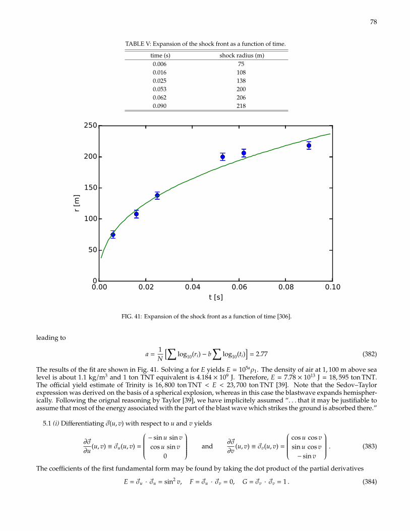
78

TABLE V: Expansion of the shock front as a function of time.

time (s) shock radius (m)0.006 750.016 1080.025 1380.053 2000.062 2060.090 218

d

da

NX

i=1

(lg(ri) a b lg(ti)

!2

= 2NX

i=1

lg(ri) a b lg(ti),

leading to

a =

Plg(ri) b

Plg(ti)

N

In [4]: a = (np.sum(yLog) - 2/5.*np.sum(xLog))/len(yLog)

print "a=", a

a= 2.77687821514

Let’s superimpose this result with the data points.

In [5]: plt.figure()

plt.errorbar(x, y, yerr=6, fmt=’o’)

plt.xlim(0, 0.1)

xFit = np.arange(0.001, 0.1, 0.001)

yFit = 10**a*xFit**(2/5.)

plt.plot(xFit, yFit)

plt.xlabel(’t [s]’)

plt.ylabel(’r [m]’)

plt.show()

Solving a for E yields

E = 105a 4

250.

The density of air at 1100 m above sea level is about 1.1 kg/m3 and 1 ton TNT equivalent is 4.184 109 J.Therefore

5

FIG. 41: Expansion of the shock front as a function of time [306].

leading to

a =1N

[∑log10(ri) − b

∑log10(ti)

]= 2.77 (382)

The results of the fit are shown in Fig. 41. Solving a for E yields E = 105aρ1. The density of air at 1, 100 m above sealevel is about 1.1 kg/m3 and 1 ton TNT equivalent is 4.184 × 109 J. Therefore, E = 7.78 × 1013 J = 18, 595 ton TNT.The official yield estimate of Trinity is 16, 800 ton TNT < E < 23, 700 ton TNT [39]. Note that the Sedov–Taylorexpression was derived on the basis of a spherical explosion, whereas in this case the blastwave expands hemispher-ically. Following the orignal reasoning by Taylor [39], we have implicitely assumed “. . . that it may be justifiable toassume that most of the energy associated with the part of the blast wave which strikes the ground is absorbed there.”

5.1 (i) Differentiating ~σ(u, v) with respect to u and v yields

∂~σ∂u

(u, v) ≡ ~σu(u, v) =

− sin u sin vcos u sin v

0

and∂~σ∂v

(u, v) ≡ ~σv(u, v) =

cos u cos vsin u cos v− sin v

. (383)

The coefficients of the first fundamental form may be found by taking the dot product of the partial derivatives

E = ~σu · ~σu = sin2 v, F = ~σu · ~σv = 0, G = ~σv · ~σv = 1 . (384)

79

The line element may be expressed in terms of the coefficients of the first fundamental form as ds2 = sin2 v du2 + dv2.(ii) The surface area is given by

A =

∫ π

0

∫ 2π

0

√

EG − F2du dv =

∫ π

0

∫ 2π

0sin v du dv = 2π(− cos v)

∣∣∣∣∣∣π

0

= 4π . (385)

The coefficients of the second fundamental form are

e = ~σuu · n = sin2 v, f = ~σuv · n = 0, g = ~σvv · n = 1 . (386)

(iii) The Gaussian curvature is

K =det IIdet I

=eg − f 2

EG − F2 = 1 . (387)

5.2 (i) The coefficients of the first fundamental form are

E = tanh2 u, F = 0, G = sech2 u . (388)

The line element is ds2 = tanh2 u du2 + sech2 u dv2. (ii) The surface area is

A = 2∫ 2π

0

∫∞

0sechu tanhu du dv = 4π (389)

which is exactly that of the sphere. (iii) The coefficients of the second fundamental form are

e = −sechu tanhu, f = 0, g = sechu tanhu . (390)

The Gaussian curvature is K = −1.

5.3 We have

ddt||γ||2 =

ddt

(~γ · ~γ) = 2~γ · ~γ . (391)

Since γ is geodesic, ~γ is perpendicular to the tangent plane which contains ~γ. Hence, ~γ · ~γ = 0. Subsequently,d||γ||2/dt = 0. Therefore, the speed ||γ|| is constant.

5.4 The tangent plane is spanned by ~σu and ~σv. By definition the curve γ is a geodesic if ~γ · ~σu = ~γ · ~σv = 0. Since~γ = u~σu + v~σv, it follows that ~γ · ~σu = 0 becomes[

ddt

(u~σu + v~σv)]· ~σu = 0 . (392)

We rewrite the left hand side of the above equation:[ddt

(u~σu + v~σv)]· ~σu =

ddt

[(u~σu + v~σv) · ~σu

]− (u~σu + v~σv) ·

d~σu

dt

=ddt

(Eu + Fv) − (u~σu + v~σv) · (u~σuu + v~σuv)

=ddt

(Eu + Fv) −[u2(~σu · ~σuu) + uv(~σu · ~σuv + ~σv · ~σuu) + v2(~σv · ~σuv)

]. (393)

We have that

~σu · ~σuu =12∂∂u

(~σu · ~σu) =12

Eu, ~σv · ~σuv =12

Gu, ~σu · ~σuv + ~σv · ~σuu = Fu . (394)

Substituting them into (393), we obtain[ddt

(u~σu + v~σv)]· ~σu =

ddt

(Eu + Fv) −12

(Euu2 + 2Fuuv + Guv2) . (395)

80

This establishes the first differential equation (113). Similarly, (114) can be established from[ddt

(u~σu + v~σv)]· ~σv = 0 . (396)

5.5 For the parametrization in (115) the first fundamental form is found to be ds2 = dθ2 + cos2 θdφ2, with E = 1,F = 0, and G = cos2 θ. We restrict to unit-speed curves γ(t) = ~σ(θ(t), φ(t)), so that

Eθ2 + 2Fθφ + Gφ2 = θ2 + φ2 cos2 θ = 1 . (397)

If γ is a geodesic, then (114) is satisfied. Here (114) reduces to

ddt

(φ cos2 θ) = 0, or equivalently φ cos2 θ = ζ, (398)

where ζ is a constant. There are two cases: (i) ζ = 0; then φ = 0. In this case, φ is constant and γ is part of a meridian.(ii) ζ , 0. Substituting (398) into the unit-speed condition (397), we have

θ2 = 1 −ζ2

cos2 θ. (399)

Combining the above with (398), along the geodesic it holds that(dφdθ

)2

=φ2

θ2=

1cos2 θ(cos2 θ/ζ2 − 1)

. (400)

Integrate the derivative dφ/dθ:

φ − φ0 = ±

∫dθ

cosθ√

cos2 θ/ζ2 − 1, (401)

where φ0 is a constant. The substitution u = tanθ yields

φ − φ0 = ±

∫du√

ζ−2 − 1 − u2= sin−1

u√ζ−2 − 1

, (402)

which leads to

tanθ = ± sin(φ − φ0)√ζ−2 − 1 . (403)

Multiply both sides of the above equation by cosθ:

sinθ = ±√ζ−2 − 1(cosφ0 cosθ sinφ − sinφ0 cosθ cosφ) . (404)

Since ~σ(θ, φ) = (xy, z), we have

z = ∓(sinφ0

√ζ−2 − 1) x ± (cosφ0

√ζ−2 − 1) y . (405)

Clearly, z = 0 when x = y = 0. Therefore, γ is contained in the intersection of S2 with a plane through the center ofthe sphere. Hence it is part of a great circle.

5.6 (132) gives the rate at which a clock at radius r ticks relative to one infinitely far away. Here we are asked tocompare the rate of a clock at radius r relative to one at the radius of the Earth (i.e., at the Earth’s surface). We canthink about this by considering the rate of each of these clocks relative to a distant clock. That is, the clock on theEarth’s surface has a rate a factor √

1 −1c2

2GM⊕R⊕

(406)

81

slower than the distant clock, while the clock at radius r has a rate√1 −

1c2

2GM⊕r

. (407)

Note that both these expressions are less than one, but because r > R⊕, the stationary clock at radius r ticks fasterthan that at the Earth’s surface. Indeed, the relative rate of the two is just the ratio of these two expressions√(

1 −1c2

2GM⊕r

) (1 −

1c2

2GM⊕R⊕

)−1

. (408)

Again, the expression in (408) is greater than 1. (ii) Circular motion at speed v at a radius r gives rise to an accelerationv2/r, which we know is due to gravity. Thus if the astronaut has a mass m, Newton’s second law yields

GM⊕mr2 = m

v2

r, or solving for v gives v =

√GM⊕

r. (409)

The time dilation in special relativity is due to the by now familiar factor (1 − v2/c2)1/2, which gives√1 −

GM⊕rc2 . (410)

Note again how similar this looks to the expression above for time dilation due to gravity. Again, this is the rate thatan orbiting clock at radius r ticks relative to a stationary clock at the same radius. (iii) In part (408), we calculatedthe ratio of rates of stationary clocks at radius r and R⊕ (due to general relativity), while in part (410), we calculatedthe ratio of the rates of an orbiting clock at radius r to a stationary clock at the same radius. Therefore, the ratio ofthe rate of an orbiting clock at radius r to a stationary one on the ground is simply the product of these two results;namely, √(

1 −2GM⊕

rc2

) (1 −

2GM⊕R⊕c2

)−1 (1 −

GM⊕rc2

). (411)

(iv) We now simplify (411). We will do this in pieces, starting from (408) we can write:√(1 −

1c2

2GM⊕r

) (1 −

1c2

2GM⊕R⊕

)−1

≈

√(1 −

1c2

2GM⊕r

) (1 +

1c2

2GM⊕R⊕

+ · · ·

). (412)

We then use (1 − x)(1 − y) ≈ 1 − (x + y) to re-write (412) as√1 −

GM⊕c2

(2r−

2R⊕

). (413)

This then gets multiplied by (410), yielding√1 −

GM⊕c2

(3r−

2R⊕

)≈ 1 −

GM⊕2c2

(3r−

2R⊕

). (414)

However, we do need to justify the use of the various approximations we have made. We dealt with a variety ofexpressions of the form 1 − x; in every case x is of the form (GM⊕)/(rc2). The smallest r we considered, and thereforethe largest the expression (GM⊕)/(rc2), is r = R⊕. So we plug in numbers at r = R⊕ to obtain

GM⊕R⊕c2 =

23

10−10 m3 s−2 kg−1× 6 × 1024 kg

6.4 × 106 m × (3 × 108 m/s)2 ≈ 7 × 10−9 , (415)

which is indeed a number much much smaller than 1. (v) We are asked to find the radius at which (414) isequal to unity. This clearly holds when 3/r − 2/R⊕ = 0, or r = 1.5R⊕. Given the radius of the Earth is 6, 400 km,

82

the critical radius r = 1.5R⊕ is at a distance of 9, 600 km from the Earth’s center, or 3, 200 km above the Earth’ssurface. Now, (414) is less than 1 for r < 1.5R⊕, and so astronauts on the space shuttle age less than those staying home.

5.7 (i) The Schwarzschild radius of a black hole of mass M is RSch = 2GM/c2. The volume of a sphere of this radiusis just the familiar 4πR3

Sch. The density is the mass divided by the volume, giving:

ρBH = M ×[

43π

(2GMc2

)3]−1

=3c6

32πG3M2 . (416)

The more massive the black hole, the smaller the density. Thus there is a mass at which the black hole has the densityof paper, which is what we are trying to figure out. (ii) The density is the mass per unit volume. If we can figure outthe volume of a square meter of paper (whose mass we know, 75 g), we can calculate its density. The volume of apiece of paper is its area times its thickness. The thickness is 0.1 mm, or 10−4 m, and so the volume of a square meterof paper is 10−4 m3. Therefore, the density of paper is

ρ =7.5 × 10−2 kg

10−4 m3 = 7.5 × 102 kg/m3 , (417)

similar to (but slightly less than) the density of water (remember, paper is made of wood, and wood floats in water).(iii) Here we equate (416) with (417) and solve for the mass

M =

√3c6

32πG3ρ≈ 3 × 1038 kg , (418)

where we have made all the usual approximations of π = 3, 32 = 10, and so on. We need to express this in solarmasses, so we divide by M = 2 × 1030 kg to obtain M ≈ 1.5 × 108M. A black hole 150 million times the mass of theSun has the same density as a piece of paper. We know the Hitchhiker’s Guide to the Galaxy is science fiction, butdo such incredibly massive black holes actually exist? Indeed they do: the cores of massive galaxies (including ourown Milky Way) do contain such enormous black holes. Actually, the most massive such black hole known to existis in the core of a particularly luminous galaxy known as M87, with a mass of 3 billion solar masses. We still have tocalculate the Schwarzschild radius of a black hole. We could plug into the formula for a Schwarzschild radius andcalculate away, but here we outline a simpler approach. We know the Schwarzschild radius is proportional to themass of a black hole, and we happen to remember that a M mass black hole has a Schwarzschild radius of 3 km,(129). So a 150 million M black hole has a Schwarzschild radius 150 million times larger, or 4.5 × 108 km. We areasked to express this in terms of AU; 1 AU = 1.5 × 108 km, so the Schwarzschild radius of such a black hole is 3 AU.(iv) We know the entire mass of the black hole. If we can calculate the mass of a single piece of paper, the ratio ofthe two gives the total number of pages. So we now turn to calculate the mass of a single piece of paper. We knowthat a square meter of paper has a mass of 75 g. How many square meters is a standard-size sheet? One inch is2.5 cm = 2.5 × 10−2 m. So 8.5 × 11 inch2

≈ 100 inch2≈ 6 × 10−2 m−2. Thus the mass is

Mass of a piece of paper = 7.5 × 10−2 kg/m2× 6 × 10−2 m2

≈ 5 × 10−3 kg. (419)

That is, a piece of paper weighs about 5 g. We divide this into the mass we calculated above:

Number of sheets of paper =Mass of rule book

Mass per page=

3 × 1038 kg5 × 10−3 kg/page

= 6 × 1040 pages . (420)

Strictly speaking, if the rule book is printed on both sides of the page, we should multiply the above result by afactor of two. That is one seriously long set of rules! Finally, note that because the density of a more massive blackhole is smaller (416), the mass and number of pages of the Brockian Ultra Cricket rule book as given by (420) is reallyjust a lower limit. That is, if the rule book were even larger than what we have just calculated, it would still collapseinto a black hole.

5.8 (i) The Schwarzschild radius of a 3M black hole is RSch = 2GM/c2 = 9 km. If you remember that for 1 M blackhole the Schwarzchild radius is 3 km, you can scale from there. (ii) Using the Newton’s law of gravitation, we canwrite the difference in gravitational forces acting on two bodies of mass m which are located at distances r1 and r2from the massive body of mass M

δF ≡ F1 − F2 =GmM

r21

−GmM

r22

= GmM

1r2

1

−1r2

2

. (421)

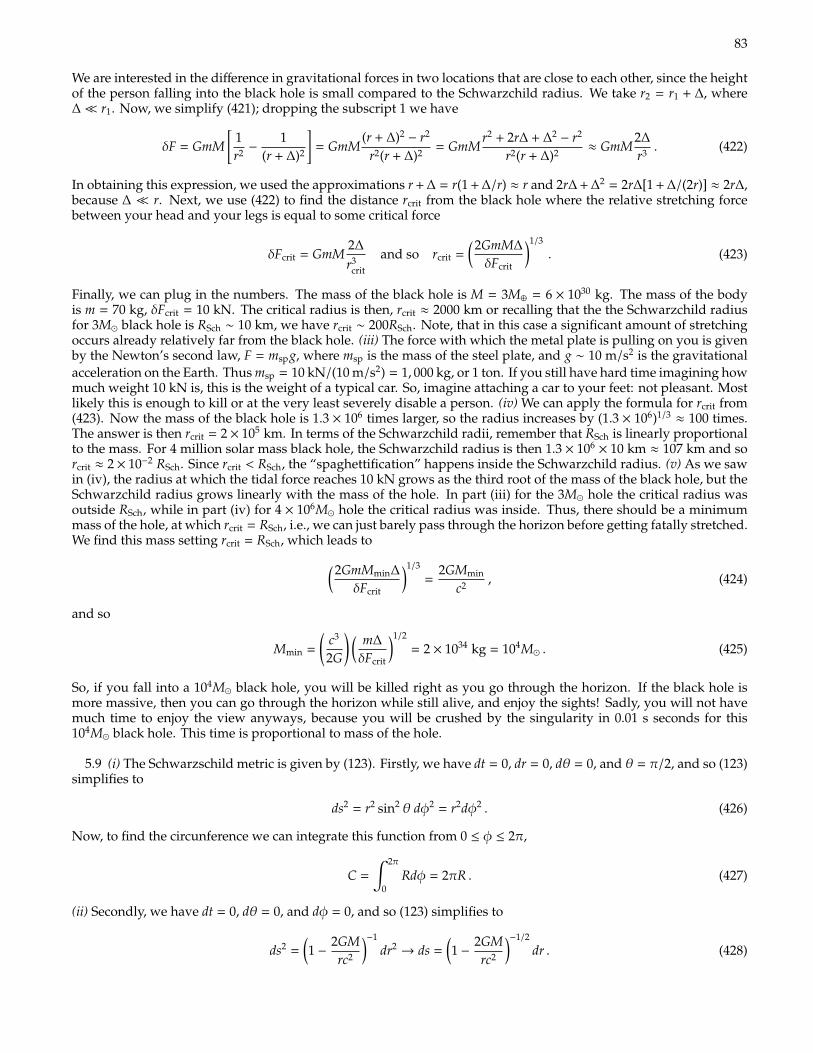
83

We are interested in the difference in gravitational forces in two locations that are close to each other, since the heightof the person falling into the black hole is small compared to the Schwarzchild radius. We take r2 = r1 + ∆, where∆ r1. Now, we simplify (421); dropping the subscript 1 we have

δF = GmM[

1r2 −

1(r + ∆)2

]= GmM

(r + ∆)2− r2

r2(r + ∆)2 = GmMr2 + 2r∆ + ∆2

− r2

r2(r + ∆)2 ≈ GmM2∆

r3 . (422)

In obtaining this expression, we used the approximations r + ∆ = r(1 + ∆/r) ≈ r and 2r∆ + ∆2 = 2r∆[1 + ∆/(2r)] ≈ 2r∆,because ∆ r. Next, we use (422) to find the distance rcrit from the black hole where the relative stretching forcebetween your head and your legs is equal to some critical force

δFcrit = GmM2∆

r3crit

and so rcrit =(2GmM∆

δFcrit

)1/3

. (423)

Finally, we can plug in the numbers. The mass of the black hole is M = 3M⊕ = 6 × 1030 kg. The mass of the bodyis m = 70 kg, δFcrit = 10 kN. The critical radius is then, rcrit ≈ 2000 km or recalling that the the Schwarzchild radiusfor 3M black hole is RSch ∼ 10 km, we have rcrit ∼ 200RSch. Note, that in this case a significant amount of stretchingoccurs already relatively far from the black hole. (iii) The force with which the metal plate is pulling on you is givenby the Newton’s second law, F = mspg, where msp is the mass of the steel plate, and g ∼ 10 m/s2 is the gravitationalacceleration on the Earth. Thus msp = 10 kN/(10 m/s2) = 1, 000 kg, or 1 ton. If you still have hard time imagining howmuch weight 10 kN is, this is the weight of a typical car. So, imagine attaching a car to your feet: not pleasant. Mostlikely this is enough to kill or at the very least severely disable a person. (iv) We can apply the formula for rcrit from(423). Now the mass of the black hole is 1.3 × 106 times larger, so the radius increases by (1.3 × 106)1/3

≈ 100 times.The answer is then rcrit = 2 × 105 km. In terms of the Schwarzchild radii, remember that RSch is linearly proportionalto the mass. For 4 million solar mass black hole, the Schwarzchild radius is then 1.3 × 106

× 10 km ≈ 107 km and sorcrit ≈ 2 × 10−2 RSch. Since rcrit < RSch, the “spaghettification” happens inside the Schwarzchild radius. (v) As we sawin (iv), the radius at which the tidal force reaches 10 kN grows as the third root of the mass of the black hole, but theSchwarzchild radius grows linearly with the mass of the hole. In part (iii) for the 3M hole the critical radius wasoutside RSch, while in part (iv) for 4 × 106M hole the critical radius was inside. Thus, there should be a minimummass of the hole, at which rcrit = RSch, i.e., we can just barely pass through the horizon before getting fatally stretched.We find this mass setting rcrit = RSch, which leads to(2GmMmin∆

δFcrit

)1/3

=2GMmin

c2 , (424)

and so

Mmin =

(c3

2G

) ( m∆

δFcrit

)1/2

= 2 × 1034 kg = 104M . (425)

So, if you fall into a 104M black hole, you will be killed right as you go through the horizon. If the black hole ismore massive, then you can go through the horizon while still alive, and enjoy the sights! Sadly, you will not havemuch time to enjoy the view anyways, because you will be crushed by the singularity in 0.01 s seconds for this104M black hole. This time is proportional to mass of the hole.

5.9 (i) The Schwarzschild metric is given by (123). Firstly, we have dt = 0, dr = 0, dθ = 0, and θ = π/2, and so (123)simplifies to

ds2 = r2 sin2 θ dφ2 = r2dφ2 . (426)

Now, to find the circunference we can integrate this function from 0 ≤ φ ≤ 2π,

C =

∫ 2π

0Rdφ = 2πR . (427)

(ii) Secondly, we have dt = 0, dθ = 0, and dφ = 0, and so (123) simplifies to

ds2 =(1 −

2GMrc2

)−1

dr2→ ds =

(1 −

2GMrc2

)−1/2

dr . (428)

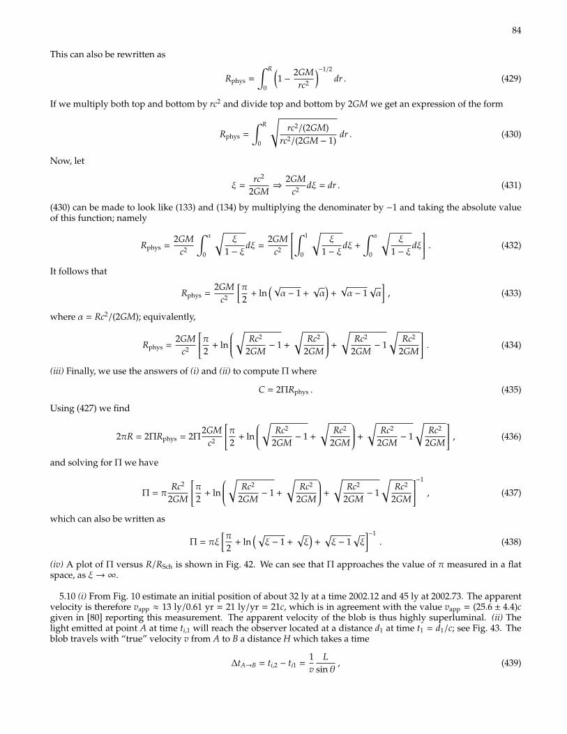
84

This can also be rewritten as

Rphys =

∫ R

0

(1 −

2GMrc2

)−1/2

dr . (429)

If we multiply both top and bottom by rc2 and divide top and bottom by 2GM we get an expression of the form

Rphys =

∫ R

0

√rc2/(2GM)

rc2/(2GM − 1)dr . (430)

Now, let

ξ =rc2

2GM⇒

2GMc2 dξ = dr . (431)

(430) can be made to look like (133) and (134) by multiplying the denominater by −1 and taking the absolute valueof this function; namely

Rphys =2GM

c2

∫ α

0

√ξ

1 − ξdξ =

2GMc2

∫ 1

0

√ξ

1 − ξdξ +

∫ α

0

√ξ

1 − ξdξ

. (432)

It follows that

Rphys =2GM

c2

[π2

+ ln(√α − 1 +

√α)

+√

α − 1√α], (433)

where α = Rc2/(2GM); equivalently,

Rphys =2GM

c2

π2 + ln

√

Rc2

2GM− 1 +

√Rc2

2GM

+

√Rc2

2GM− 1

√Rc2

2GM

. (434)

(iii) Finally, we use the answers of (i) and (ii) to compute Π where

C = 2ΠRphys . (435)

Using (427) we find

2πR = 2ΠRphys = 2Π2GM

c2

π2 + ln

√

Rc2

2GM− 1 +

√Rc2

2GM

+

√Rc2

2GM− 1

√Rc2

2GM

, (436)

and solving for Π we have

Π = πRc2

2GM

π2 + ln

√

Rc2

2GM− 1 +

√Rc2

2GM

+

√Rc2

2GM− 1

√Rc2

2GM

−1

, (437)

which can also be written as

Π = πξ[π2

+ ln(√ξ − 1 +

√ξ)

+√ξ − 1

√ξ]−1

. (438)

(iv) A plot of Π versus R/RSch is shown in Fig. 42. We can see that Π approaches the value of π measured in a flatspace, as ξ→∞.

5.10 (i) From Fig. 10 estimate an initial position of about 32 ly at a time 2002.12 and 45 ly at 2002.73. The apparentvelocity is therefore vapp ≈ 13 ly/0.61 yr = 21 ly/yr = 21c, which is in agreement with the value vapp = (25.6 ± 4.4)cgiven in [80] reporting this measurement. The apparent velocity of the blob is thus highly superluminal. (ii) Thelight emitted at point A at time ti,1 will reach the observer located at a distance d1 at time t1 = d1/c; see Fig. 43. Theblob travels with “true” velocity v from A to B a distance H which takes a time

∆tA→B = ti,2 − ti1 =1v

Lsinθ

, (439)

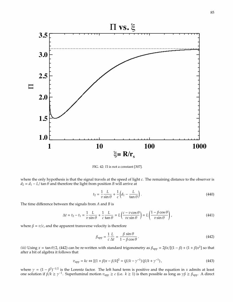
85

Π vs. ξ

1 10 100 1000 ξ≡ R/rs

1.0

1.5

2.0

2.5

3.0

3.5Π

Figure 1: 1 Plot of π versus Rrs

(d). Plot Π as a function of ξ ! R/rs for ξ " [1,103] (use log axes for the x axis). Whathappens t0 Π as ξ# ∞?

the plot is given in figure 1.

and we can see that Π approaches the true value of π that is measured in a flat space.

Problem #2 [Time to fall into a black hole]

We haven’t spent too much time discussing black holes in great detail. But take it as agiven that

a particle initially at rest at infinity follows a trajectory that always obeys

!1$ 2GM

rc2

"dt

dτ= 1

this is a constant of the motion, and is actually closely related to the total energy of the

particle.

(a). Rewrite the Schwarzschild metric in the context of a particle falling in from infinity

along a direct radial line. Your metric should only have a dτ term and a dr term.

3

FIG. 42: Π is not a constant [307].

where the only hypothesis is that the signal travels at the speed of light c. The remaining distance to the observer isd2 = d1 − L/ tanθ and therefore the light from position B will arrive at

t2 =1v

Lsinθ

+1c

(d1 −

Ltanθ

). (440)

The time difference between the signals from A and B is

∆t = t2 − t1 =1v

Lsinθ

+1c

Ltanθ

= L(c − v cosθ

vc sinθ

)= L

(1 − β cosθ

v sinθ

), (441)

where β = v/c, and the apparent transverse velocity is therefore

βapp =1c

L∆t

=β sinθ

1 − β cosθ. (442)

(iii) Using x = tanθ/2, (442) can be re-written with standard trigonometry as βapp = 2βx/[(1 − β) + (1 + β)x2] so thatafter a bit of algebra it follows that

vapp = kc⇔ [(1 + β)x − β/k]2 = (β/k − γ−1) (β/k + γ−1) , (443)

where γ = (1 − β2)−1/2 is the Lorentz factor. The left hand term is positive and the equation in x admits at leastone solution if β/k ≥ γ−1. Superluminal motion vapp ≥ c (i.e. k ≥ 1) is then possible as long as γβ ≥ βapp. A direct

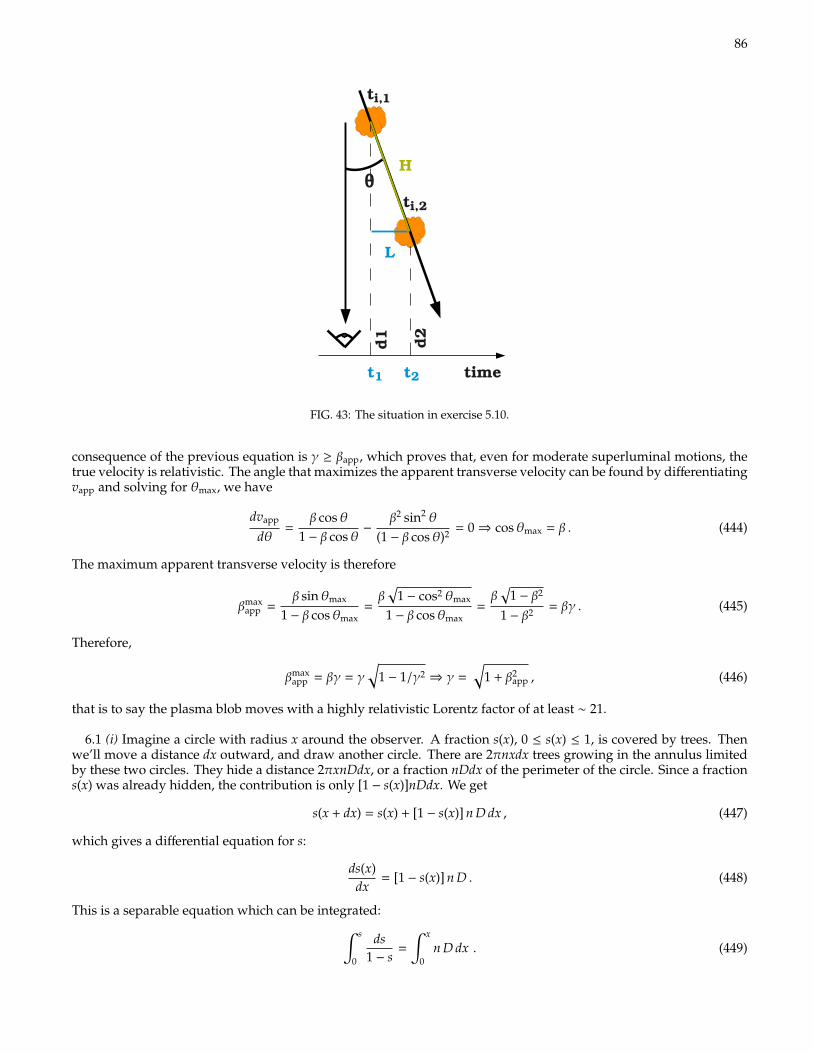
8620 1. VERY HIGH ENERGY BLAZARS

Figure 4. Schematic view of the motion of an emit-ting region along a direction at angle θ from the lineof sight. The signal emitted at ti,1 (resp. ti,2) travelsfor d1/c (resp. d2/c) before arriving at t1 (resp. t2). Adisplacement of L is observed between t1 and t2, for aneffectively travelled distance of H.

in Fig. 4. The apparent velocity vapp is given by Eq. (1.1):

(1.1) vapp =L

t2 − t1=

L

(ti,2 + d2c ) − (ti,1 + d1

c )=

L

(ti,2 − ti,1) − d1−d2c

where the only hypothesis is that the signal travels at the speed of lightc. The “true” velocity of the emitting region is vi = H/(ti,2−ti,1). Thenusing Eq. (1.1), the apparent velocity is:

(1.2) vapp =H sin θ

H/vi − H cos θ/c=

vi sin θ

1 − vic cos θ

Calling β = vi/c, and using t = tan θ/2, Eq. (1.1) can be re-writtenwith standard trigonometry vapp/c = 2βt/

£(1 − β) + (1 + β)t2

§, so

that after a bit of algebra:

(1.3) vapp = kc ⇔ [(1 + β)t − β/k]2 = (β/k − 1/γ) × (β/k + 1/γ)

past

el-0

0822

242,

ver

sion

1 -

14 M

ay 2

013

FIG. 43: The situation in exercise 5.10.

consequence of the previous equation is γ ≥ βapp, which proves that, even for moderate superluminal motions, thetrue velocity is relativistic. The angle that maximizes the apparent transverse velocity can be found by differentiatingvapp and solving for θmax, we have

dvapp

dθ=

β cosθ1 − β cosθ

−β2 sin2 θ

(1 − β cosθ)2 = 0⇒ cosθmax = β . (444)

The maximum apparent transverse velocity is therefore

βmaxapp =

β sinθmax

1 − β cosθmax=β√

1 − cos2 θmax

1 − β cosθmax=β√

1 − β2

1 − β2 = βγ . (445)

Therefore,

βmaxapp = βγ = γ

√1 − 1/γ2 ⇒ γ =

√1 + β2

app , (446)

that is to say the plasma blob moves with a highly relativistic Lorentz factor of at least ∼ 21.

6.1 (i) Imagine a circle with radius x around the observer. A fraction s(x), 0 ≤ s(x) ≤ 1, is covered by trees. Thenwe’ll move a distance dx outward, and draw another circle. There are 2πnxdx trees growing in the annulus limitedby these two circles. They hide a distance 2πxnDdx, or a fraction nDdx of the perimeter of the circle. Since a fractions(x) was already hidden, the contribution is only [1 − s(x)]nDdx. We get

s(x + dx) = s(x) + [1 − s(x)] n D dx , (447)

which gives a differential equation for s:

ds(x)dx

= [1 − s(x)] n D . (448)

This is a separable equation which can be integrated:∫ s

0

ds1 − s

=

∫ x

0n D dx . (449)

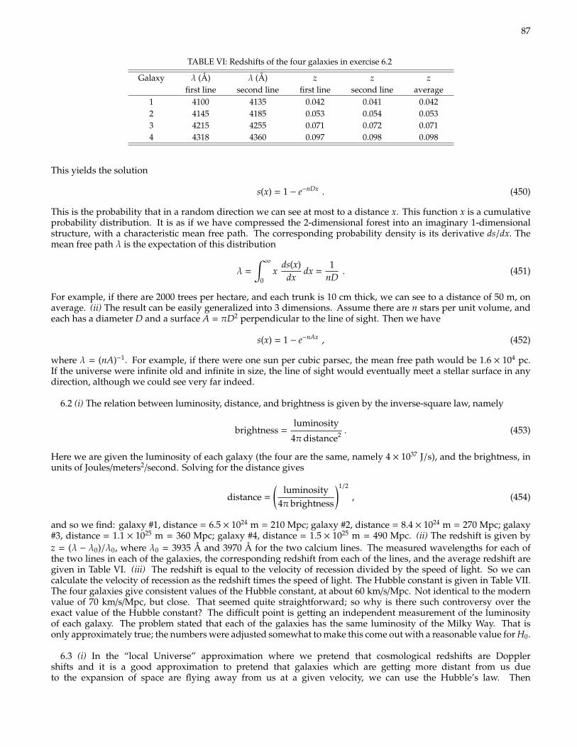
87

TABLE VI: Redshifts of the four galaxies in exercise 6.2

Galaxy λ (Å) λ (Å) z z zfirst line second line first line second line average

1 4100 4135 0.042 0.041 0.0422 4145 4185 0.053 0.054 0.0533 4215 4255 0.071 0.072 0.0714 4318 4360 0.097 0.098 0.098

This yields the solution

s(x) = 1 − e−nDx . (450)

This is the probability that in a random direction we can see at most to a distance x. This function x is a cumulativeprobability distribution. It is as if we have compressed the 2-dimensional forest into an imaginary 1-dimensionalstructure, with a characteristic mean free path. The corresponding probability density is its derivative ds/dx. Themean free path λ is the expectation of this distribution

λ =

∫∞

0x

ds(x)dx

dx =1

nD. (451)

For example, if there are 2000 trees per hectare, and each trunk is 10 cm thick, we can see to a distance of 50 m, onaverage. (ii) The result can be easily generalized into 3 dimensions. Assume there are n stars per unit volume, andeach has a diameter D and a surface A = πD2 perpendicular to the line of sight. Then we have

s(x) = 1 − e−nAx , (452)

where λ = (nA)−1. For example, if there were one sun per cubic parsec, the mean free path would be 1.6 × 104 pc.If the universe were infinite old and infinite in size, the line of sight would eventually meet a stellar surface in anydirection, although we could see very far indeed.

6.2 (i) The relation between luminosity, distance, and brightness is given by the inverse-square law, namely

brightness =luminosity

4πdistance2 . (453)

Here we are given the luminosity of each galaxy (the four are the same, namely 4 × 1037 J/s), and the brightness, inunits of Joules/meters2/second. Solving for the distance gives

distance =

(luminosity

4π brightness

)1/2

, (454)

and so we find: galaxy #1, distance = 6.5 × 1024 m = 210 Mpc; galaxy #2, distance = 8.4 × 1024 m = 270 Mpc; galaxy#3, distance = 1.1 × 1025 m = 360 Mpc; galaxy #4, distance = 1.5 × 1025 m = 490 Mpc. (ii) The redshift is given byz = (λ − λ0)/λ0, where λ0 = 3935 Å and 3970 Å for the two calcium lines. The measured wavelengths for each ofthe two lines in each of the galaxies, the corresponding redshift from each of the lines, and the average redshift aregiven in Table VI. (iii) The redshift is equal to the velocity of recession divided by the speed of light. So we cancalculate the velocity of recession as the redshift times the speed of light. The Hubble constant is given in Table VII.The four galaxies give consistent values of the Hubble constant, at about 60 km/s/Mpc. Not identical to the modernvalue of 70 km/s/Mpc, but close. That seemed quite straightforward; so why is there such controversy over theexact value of the Hubble constant? The difficult point is getting an independent measurement of the luminosityof each galaxy. The problem stated that each of the galaxies has the same luminosity of the Milky Way. That isonly approximately true; the numbers were adjusted somewhat to make this come out with a reasonable value for H0.

6.3 (i) In the “local Universe” approximation where we pretend that cosmological redshifts are Dopplershifts and it is a good approximation to pretend that galaxies which are getting more distant from us dueto the expansion of space are flying away from us at a given velocity, we can use the Hubble’s law. Then

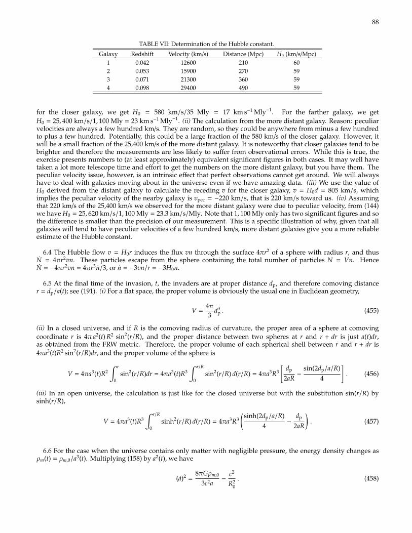
88

TABLE VII: Determination of the Hubble constant.

Galaxy Redshift Velocity (km/s) Distance (Mpc) H0 (km/s/Mpc)1 0.042 12600 210 602 0.053 15900 270 593 0.071 21300 360 594 0.098 29400 490 59

for the closer galaxy, we get H0 = 580 km/s/35 Mly = 17 km s−1 Mly−1. For the farther galaxy, we getH0 = 25, 400 km/s/1, 100 Mly = 23 km s−1 Mly−1. (ii) The calculation from the more distant galaxy. Reason: peculiarvelocities are always a few hundred km/s. They are random, so they could be anywhere from minus a few hundredto plus a few hundred. Potentially, this could be a large fraction of the 580 km/s of the closer galaxy. However, itwill be a small fraction of the 25,400 km/s of the more distant galaxy. It is noteworthy that closer galaxies tend to bebrighter and therefore the measurements are less likely to suffer from observational errors. While this is true, theexercise presents numbers to (at least approximately) equivalent significant figures in both cases. It may well havetaken a lot more telescope time and effort to get the numbers on the more distant galaxy, but you have them. Thepeculiar velocity issue, however, is an intrinsic effect that perfect observations cannot get around. We will alwayshave to deal with galaxies moving about in the universe even if we have amazing data. (iii) We use the value ofH0 derived from the distant galaxy to calculate the receding v for the closer galaxy, v = H0d = 805 km/s, whichimplies the peculiar velocity of the nearby galaxy is vpec = −220 km/s, that is 220 km/s toward us. (iv) Assumingthat 220 km/s of the 25,400 km/s we observed for the more distant galaxy were due to peculiar velocity, from (144)we have H0 = 25, 620 km/s/1, 100 Mly = 23.3 km/s/Mly. Note that 1, 100 Mly only has two significant figures and sothe difference is smaller than the precision of our measurement. This is a specific illustration of why, given that allgalaxies will tend to have peculiar velocities of a few hundred km/s, more distant galaxies give you a more reliableestimate of the Hubble constant.

6.4 The Hubble flow v = H0r induces the flux vn through the surface 4πr2 of a sphere with radius r, and thusN = 4πr2vn. These particles escape from the sphere containing the total number of particles N = Vn. HenceN = −4πr2vn = 4πr3n/3, or n = −3vn/r = −3H0n.

6.5 At the final time of the invasion, t, the invaders are at proper distance dp, and therefore comoving distancer = dp/a(t); see (191). (i) For a flat space, the proper volume is obviously the usual one in Euclidean geometry,

V =4π3

d3p . (455)

(ii) In a closed universe, and if R is the comoving radius of curvature, the proper area of a sphere at comovingcoordinate r is 4π a2(t) R2 sin2(r/R), and the proper distance between two spheres at r and r + dr is just a(t)dr,as obtained from the FRW metric. Therefore, the proper volume of each spherical shell between r and r + dr is4πa3(t)R2 sin2(r/R)dr, and the proper volume of the sphere is

V = 4πa3(t)R2∫ r

0sin2(r/R)dr = 4πa3(t)R3

∫ r/R

0sin2(r/R) d(r/R) = 4πa3R3

[dp

2aR−

sin(2dp/a/R)4

]. (456)

(iii) In an open universe, the calculation is just like for the closed universe but with the substitution sin(r/R) bysinh(r/R),

V = 4πa3(t)R3∫ r/R

0sinh2(r/R) d(r/R) = 4πa3R3

(sinh(2dp/a/R)

4−

dp

2aR

). (457)

6.6 For the case when the universe contains only matter with negligible pressure, the energy density changes asρm(t) = ρm,0/a3(t). Multiplying (158) by a2(t), we have

(a)2 =8πGρm,0

3c2a−

c2

R20

. (458)

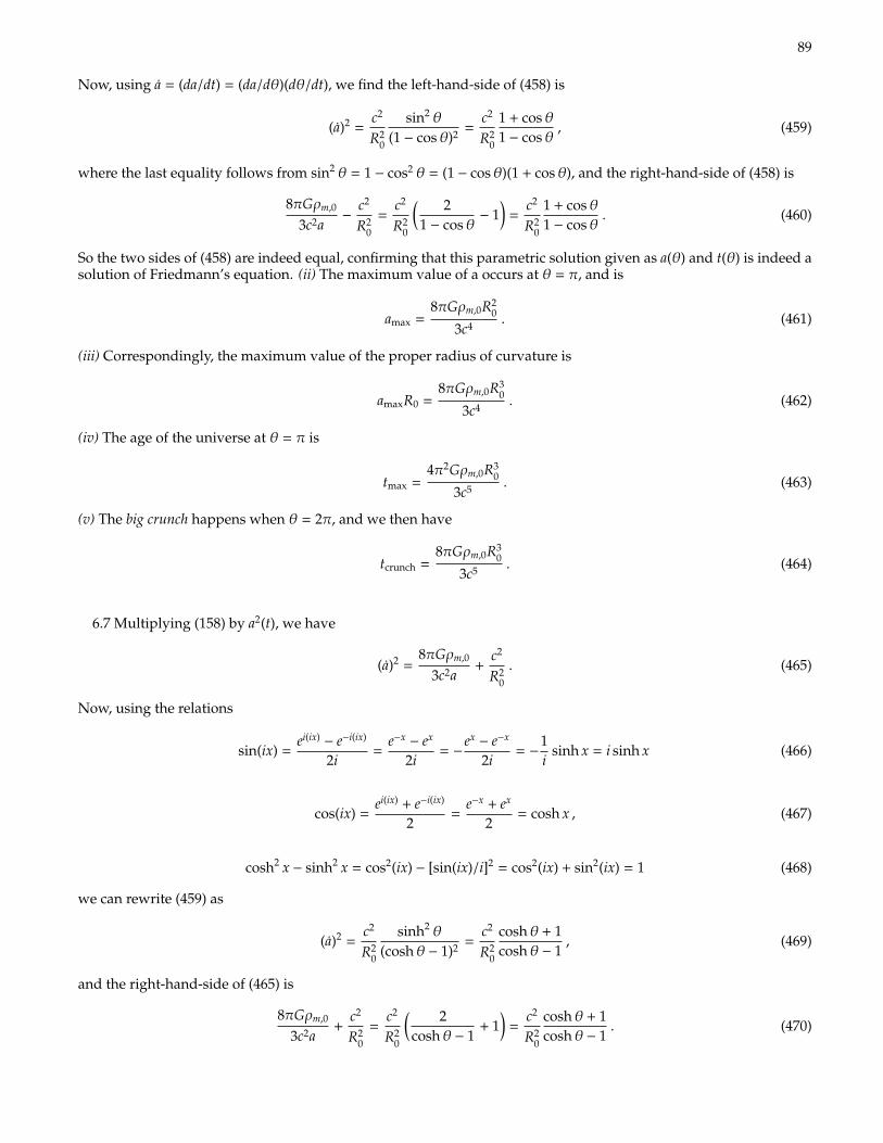
89

Now, using a = (da/dt) = (da/dθ)(dθ/dt), we find the left-hand-side of (458) is

(a)2 =c2

R20

sin2 θ

(1 − cosθ)2 =c2

R20

1 + cosθ1 − cosθ

, (459)

where the last equality follows from sin2 θ = 1 − cos2 θ = (1 − cosθ)(1 + cosθ), and the right-hand-side of (458) is

8πGρm,0

3c2a−

c2

R20

=c2

R20

( 21 − cosθ

− 1)

=c2

R20

1 + cosθ1 − cosθ

. (460)

So the two sides of (458) are indeed equal, confirming that this parametric solution given as a(θ) and t(θ) is indeed asolution of Friedmann’s equation. (ii) The maximum value of a occurs at θ = π, and is

amax =8πGρm,0R2

0

3c4 . (461)

(iii) Correspondingly, the maximum value of the proper radius of curvature is

amaxR0 =8πGρm,0R3

0

3c4 . (462)

(iv) The age of the universe at θ = π is

tmax =4π2Gρm,0R3

0

3c5 . (463)

(v) The big crunch happens when θ = 2π, and we then have

tcrunch =8πGρm,0R3

0

3c5 . (464)

6.7 Multiplying (158) by a2(t), we have

(a)2 =8πGρm,0

3c2a+

c2

R20

. (465)

Now, using the relations

sin(ix) =ei(ix)− e−i(ix)

2i=

e−x− ex

2i= −

ex− e−x

2i= −

1i

sinh x = i sinh x (466)

cos(ix) =ei(ix) + e−i(ix)

2=

e−x + ex

2= cosh x , (467)

cosh2 x − sinh2 x = cos2(ix) − [sin(ix)/i]2 = cos2(ix) + sin2(ix) = 1 (468)

we can rewrite (459) as

(a)2 =c2

R20

sinh2 θ

(coshθ − 1)2 =c2

R20

coshθ + 1coshθ − 1

, (469)

and the right-hand-side of (465) is

8πGρm,0

3c2a+

c2

R20

=c2

R20

( 2coshθ − 1

+ 1)

=c2

R20

coshθ + 1coshθ − 1

. (470)

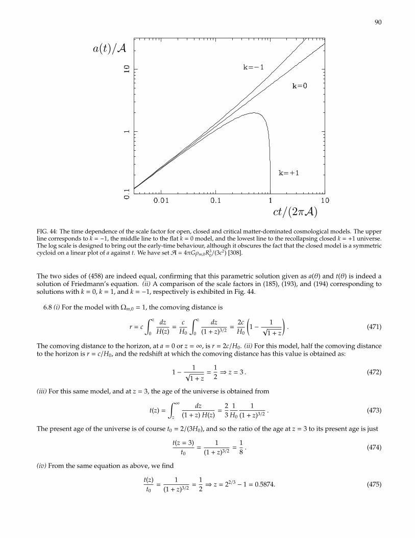
90

Figure 3. The time dependence of the scale factor for open, closed and criticalmatter-dominated cosmological models. The upper line corresponds to k = °1, themiddle line to the flat k = 0 model, and the lowest line to the recollapsing closedk = +1 universe. The log scale is designed to bring out the early-time behaviour,although it obscures the fact that the closed model is a symmetric cycloid on alinear plot of R against t.

5.4 Radiation-dominated universe

The universe cannot be dominated by matter at early times, because it contains some relativisticparticles (photons). The number density of particles of all kinds scale as n / R°3. However, theenergy (and hence mass) of relativistic particles is redshifted, thus obeying E / R°1. Therefore,the energy-mass density corresponding to radiation scales as Ω / R°4, rather than the Ω / R°3

law for pressureless matter. This shows us that the early universe was inevitably radiationdominated: even if radiation makes a very small contribution to the overall mass budget of theuniverse today, it would have been relatively more important in the past. There must have beena time at which the densities in matter and radiation were equal, with the radiation dominatingat early times and the matter at later times.

We already solved Friedmann’s equation for pressureless matter. If we include radiation,we may as well stick to the simplest case, which is the k = 0 flat universe. This will always be agood approximation to the early phases of the universe, as can be seen by going back to the basicform of Friedmann’s equation: R2 = 8ºGΩR2/3°kc2. For matter and radiation, ΩR2 / R°1 andR°2 respectively. At small R, the density term therefore completely overwhelms the curvature

16

a(t)/A

ct/(2A)

FIG. 44: The time dependence of the scale factor for open, closed and critical matter-dominated cosmological models. The upperline corresponds to k = −1, the middle line to the flat k = 0 model, and the lowest line to the recollapsing closed k = +1 universe.The log scale is designed to bring out the early-time behaviour, although it obscures the fact that the closed model is a symmetriccycloid on a linear plot of a against t. We have setA = 4πGρm,0R3

0/(3c2) [308].

The two sides of (458) are indeed equal, confirming that this parametric solution given as a(θ) and t(θ) is indeed asolution of Friedmann’s equation. (ii) A comparison of the scale factors in (185), (193), and (194) corresponding tosolutions with k = 0, k = 1, and k = −1, respectively is exhibited in Fig. 44.

6.8 (i) For the model with Ωm,0 = 1, the comoving distance is

r = c∫ z

0

dzH(z)

=c

H0

∫ z

0

dz(1 + z)3/2

=2cH0

(1 −

1√

1 + z

). (471)

The comoving distance to the horizon, at a = 0 or z = ∞, is r = 2c/H0. (ii) For this model, half the comoving distanceto the horizon is r = c/H0, and the redshift at which the comoving distance has this value is obtained as:

1 −1

√1 + z

=12⇒ z = 3 . (472)

(iii) For this same model, and at z = 3, the age of the universe is obtained from

t(z) =

∫∞

z

dz(1 + z) H(z)

=23

1H0

1(1 + z)3/2

. (473)

The present age of the universe is of course t0 = 2/(3H0), and so the ratio of the age at z = 3 to its present age is just

t(z = 3)t0

=1

(1 + z)3/2=

18. (474)

(iv) From the same equation as above, we find

t(z)t0

=1

(1 + z)3/2=

12⇒ z = 22/3

− 1 = 0.5874. (475)

91

Note that all these equations are of course valid only for the specific model that is flat and contains only matter, withΩm,0 = 1.

7.1 The flux of one of these objects is F = L/(4πd2L), and its angular size is θ = `/dA. Hence, the apparent surface

brightness is I ∝ F /θ2, or

I = constant ×F

θ2 = constant ×d2

A

d2L

= constant × (1 + z)−4 , (476)

where in the last equality we have used (226). Note that L, `, and 4π are constants and so can be absorbed inthe constant of proportionality. Therefore, the apparent surface brightness I will always decrease with redshift as(1 + z)−4 compared to the intrinsic surface brightness B, without any dependence on the cosmological model.

7.2 (i) The number density of photons per unit frequency is equal to the energy density per unit frequency dividedby hν, or

nνdν =8πν2dν

c3exp[hν/(kT)] − 1. (477)

The total number density is found by integrating over frequency, which gives

n =8πc3

∫ν2dν

exp[hν/(kT)] − 1. (478)

Substituting x = hν/(kT), we find

n =8πc3

(kTh

)3 ∫x2dx

ex − 1. (479)

For T0 = 2.725, we find 410.4 cm−3. (ii) The current density of baryons must then be

nb = 5.5 × 10−10 410.4 cm−3 = 2.25 × 10−7 cm−3 . (480)

(iii) Every baryon weighs approximately like the mass of a proton (this is not exact because, for example, the heliumnuclei weigh a little less than 4 protons because of the helium nucleus binding energy, but the difference is rathersmall). So the density of baryons is nbmp = 3.78 × 10−31g/cm3. The critical density is 3H2

0/(8πG) = 9.2 × 10−30 g/cm3,so Ωb = 0.041.

7.3 To analyze the measurement of our own galaxy through the CMB, it is useful to consider the density Nγ(~p )of photons in phase space, defined by specifying that there are Nγ(~p )d3p photons of each polarization (right or leftcircularly polarized) per unit spatial volume in a momentum-space volume d3p centered at ~p. Since |~p | = hν/c and4πh3ν2dν/c3 is the momentum-space volume between frequencies ν and dν, (477) gives

Nγ(~p ) =12

nT(c|~p |)/h)4πh3ν2/c3 =

1h3

1exp[|~p|c/(kT) − 1]

, (481)

where nT is the number density of photons in equilibrium with matter at temperature T at photon frequency betweenν and ν + dν, and the factor 1/2 takes account of the fact that nT includes both possible polarization states. This isof course the density that would be measured by an observer at rest in the radiation background. The phase spacevolume is Lorentz invariant, and the number of photons is also Lorentz invariant, so Nγ is a scalar, in the sense thata Lorentz transformation to a coordinate system moving with respect to the radiation background that takes ~p to ~p ′also takes Nγ to N′γ , where

N′γ(~p ′) = Nγ(~p ) . (482)

If the Earth is moving in the x-direction with a velocity (in units of c) of β, and we take ~p to be the photon momentumin the frame at rest in the CMB and ~p ′ to be the photon momentum measured on Earth, then from (42) it follows that

|~p ′| = γ(1 − β cosθ)|~p | (483)

92

where θ is the angle between p and the x-axis. Thus

N′γ(~p ′) =1h3

1exp[|~p ′|c/(kT′)] − 1

, (484)

where the temperature is a function of the angle between the direction of the photon and the Earth’s velocity

T = T′γ(1 − β cosθ) . (485)

This means that the temperature T(θ) observed in the direction θ, is given in terms of the average temperature T0 by

T(θ) = T0

√1 − β2

1 − β cosθ= T0

(1 − β2

)1/2 (1 − β cosθ

)−1≈ T0

(1 − β2/2 + · · ·

) (1 + β cosθ + β2 cos2 θ + · · ·

)≈ T0

[1 + β cosθ + β2

(cos2 θ − 1/2

)+ · · ·

]. (486)

Using the trigonometric relation cos2 x = (1 + cos 2x)/2 we obtain (240). The motion of the observer (us) gives rise toboth a dipole and other, higher order corrections. The observed dipole anisotropy implies that [109]

~v − ~vCMB = 370 ± 10 km/s towards φ = 267.7 ± 0.8, θ = 48.2 ± 0.5 , (487)

where θ is the colatitude (polar angle) and it is in the range 0 ≤ θ ≤ π and φ is the longitude (azimuth) and it is inthe range 0 ≤ φ ≤ 2π. Allowing for the Sun’s motion in the Galaxy and the motion of the Galaxy within the LocalGroup, this implies that the Local Group is moving with

~vLG − ~vCMB ≈ 600 km/s towards φ = 268, θ = 27 . (488)

This “peculiar” motion is subtracted from the measured CMB radiation, after which the intrinsic anisotropy isisolated (Fig. 23), and revealed to be about few parts in 105. Even though miniscule, these primordial perturbationsprovided seeds for the structure of the Universe.

7.4 For a discrete set of directions in the sky, the normalized intensity function is I(Ω) = 1N

∑Ni=1 δ(~ui,Ω). The

spherical harmonic coefficients acan be written as

aml =

1N

N∑i=1

Ym∗l (~ui) , (489)

where ~ui is the unit vector to the ith direction, 1 ≤ i ≤ N. Next, we construct an estimation of the correspondingpower spectrum by squaring the am

l ’s followed by a sum over m:

Cl ≡1

2l + 1

∑|m|≤l

|aml |

2 =1

N2(2l + 1)

∑|m|≤l

∣∣∣∣∣∣∣N∑

i=1

Ym∗l (~ui)

∣∣∣∣∣∣∣2

. (490)

Because all the sums are finite they could be rearranged and expanded to

Cl =1

N2(2l + 1)

N∑i=1

∑|m|≤l

|Yml (~ui)|2 +

2N2(2l + 1)

∑i< j

∑|m|≤l

Ym∗l (~ui)Ym

l (~u j) . (491)

The formula for addition of spherical harmonics is given by [111]

Pl(~x · ~y) =4π

2l + 1

∑|m|≤l

Ym∗l (~x)Ym

l (~y) . (492)

Now, since Pl(1) = 1 we set the unit direction vectors ~x and ~y to be equal in (492) to obtain

2l + 14π

=∑|m|≤l

|Yml (~x)|2 . (493)

93

Combining (491), (492), and (493) leads to

C` =1

4πN+

12πN2

∑i< j

Pl(~ui · ~u j) . (494)

Experimentally, only aml and Cl could be measured, but these are estimates of their continuous counterparts am

l ,Clrespectively. Therefore, since inner products are invariant under rotations, it follows that the Cl are also invariantunder rotations [309].

7.5 (i) The circumference of a circle of radius a is 2πa, so the orbital speed is the circumference divided by period:

v =2πaT

=2πa√

4π2a3/(GM)=

√GM

a. (495)

(ii) According to the Birkoff’s theorem, the orbit about a mass distributed within a sphere is the same as if the mass isall concentrated in the center of the sphere. So, we can use the velocity formula derived in (i), and invert it to obtainthe mass enclosed by an orbit:

M(a) =aG

v2 . (496)

The enclosed mass at 8 kpc is then M(8 kpc) ≈ 2 × 1041 kg = 1011M. (iii) If the mass enclosed by the orbit stays at1011M as the radius increases, which follows from the fact that the Sun is at the edge of the luminous galaxy, then atdifferent radii the velocity given by (496) will decrease with square root of the distance. At 30 kpc, it is v ≈ 110 km/s.At 100 kpc, we have v ≈ 60 km/s. (iv) Let’s look again at (496), which says that if the orbital velocity stays the same,the mass enclosed will increase linearly with a as the radius of the orbit grows. We already calculated the massenclosed by 8 kpc orbit in part (ii). So, at 30 kpc, the mass enclosed will be 30 kpc/8 kpc times larger, or 3.8× 1011M.At 100 kpc, the mass enclosed will 100 kpc/8 kpc times larger, or 1.3 × 1012M. (v) We see that the mass of thegravitating matter is increasing linearly with radius, and exceeds by more than factor of 10 the mass of the luminousmatter (e.g. stars and gas). We thus infer that the outer halo of the galaxy is dominated by invisible dark matter.

7.6(i) The total mass inside R is obtained from GM(R)/R = v2c (R). The answer can of course be found by substituting

for the value of G and everything else in your favorite system of units, and if you are lucky not to make any mistakeyou may even get the right answer. Often, it is faster and safer to work it out using proportionality comparing to anexample that you know and love. What could this example be but the Earth moving around the Sun? For the Earth,with M and an orbit of 1 AU the velocity is 30 kms−1 (if you did not know how fast the Earth moves around theSun, this is a good number to remember). So, the mass inside radius R is

M(R) = 8 × 1010M (497)

(ii) If the density at R is ρ0, then the density at any other radius r is ρ0(R/r)2, so the mass inside R is

M(R) = 4π∫ R

0drr2ρ0

(Rr

)2

= 4πρ0R3 . (498)

Hence the density at R is

ρ0 =M(R)4πR3 = 0.51 mp cm−3 . (499)

The result is most easily computed remembering that the solar mass contains 1.19 × 1057 proton masses (anotheruseful number to remember), and a parsec is 3.086 × 1016 m. (iii) The density is

ρΛ = ΩΛ

3H20

8πG= 5.5 × 10−6 ΩΛ mp cm−3 = 4 × 10−6 mp cm−3 . (500)

(iv) Because the dark energy is spread out uniformly, whereas the dark matter and baryonic matter are highlyconcentrated in the inner parts of galaxies, the density of dark energy is very small compared to the density of matterinside the radius of the solar orbit in the Milky Way. The dark energy therefore must have a tiny dynamical effect.

94

7.7 The relation between the emitted Tem and the observed Tobs is

Tem = Tobs(1 + z) =2.9 × 10−3 mK

λobsmax

(1 + z) , (501)

where in the last equality we used Wien’s displacement law [17]. For λobsmax = 180 µm and z = 2, we have Tem ' 48 K.

If we did not account for redshift, we would have thought the galaxy was only at 16 K.

7.8 In the benchmark model, at the present moment, the ratio of the vacum energy density to the energy densityin matter is

ρΛ

ρm,0=

ΩΛ

Ωm,0≈ 2.3 . (502)

In the past, however, when the scale factor was smaller, the ratio of densities was

ρΛ

ρm(a)=

ρΛ

ρm,0/a3 =ρΛ

ρm,0a3 . (503)

If the universe has been expanding from an initial very dense state, at some moment in the past, the energy densityof matter and Λ must have been equal. This moment of matter-Λ equality occurred when

a3mΛ =

Ωm,0

ΩΛ=

Ωm,0

1 −Ωm,0≈ 0.43 . (504)

where we have used the normalization a0 = 1 for the present. Next, we generalize (205) to write the age of theuniverse at any redshift z, for a flat model with matter and a cosmological constant,

t(z) =1

H0

∫∞

z

dz

(1 + z)√

Ωm,0(1 + z)3 + ΩΛ

=1

H0√

ΩΛ

∫∞

z

dz

(1 + z)√

1 + (Ωm,0/ΩΛ)(1 + z)3. (505)

With the change of variables y =√

1 + (Ωm,0/ΩΛ)(1 + z)3 we find 2ydy = 3(y2− 1)dz/(1 + z) and so

t =2

3H0√

ΩΛ

∫∞

y

dyy2 − 1

. (506)

The integral can be solved analytically as:

−

∫dy

y2 − 1=

12

ln[

y + 1y − 1

], (507)

which yields for t

t =2

3H0√

ΩΛ

ln

1√y2 − 1

+y√

y2 − 1

∣∣∣∣∣∣∣√

1+Ωm,0(1+z)3/ΩΛ

∞

=2

3H0√

ΩΛ

ln

√

ΩΛ

Ωm,0(1 + z)3 +

√1 +

ΩΛ

Ωm,0(1 + z)3

. (508)

Using (203) and (504) we can rewrite (508) as

H0t =2

3√

1 −Ωm,0ln

[(a/amΛ)3/2 +

√1 + (a/amΛ)3

]=

2

3√

1 −Ωm,0ln A , (509)

and so

H0t0 =2

3√

1 −Ωm,0ln A0 , (510)

95

where we have defined

A0 = a−3/2mΛ

+√

1 + a−3mΛ' 3.35 . (511)

Now, we want to find the value of a for which t = t0/2. This implies

ln A =12

ln A0 , (512)

where

A = x +√

1 + x2 with x =( a

amΛ

)3/2. (513)

(512) implies A =√

A0 and so

x +√

1 + x2 =√

A0 ⇒ 1 + x2 =(√

A0 − x)2

⇒ x =A0 − 1

2√

A0' 0.64 , (514)

yielding

a = amΛx2/3 = 0.56 and z =1a− 1 = 0.78 . (515)

We see that the redshift at which the age of the universe was half the present age is larger in this benchmark modelthan in the model with Ωm,0 = 1, see (475). This is because in the benchmark model, which contains vacuum energy,the universe has started to accelerate recently, roughly since the epoch at a = amΛ. The universe took a longer time toexpand to a = 0.56 and then it picked up speed again in its expansion up to the present a0 = 1.

8.1 We have seen in (282) that sγ ∝ T3, so that Sγ ∝ VT3. For a reversible adiabatic expansion, the entropy of the(non-interacting) CMB photons remains unchanged. Hence, when V doubles, T will decrease by a factor (2)−1/3. Soafter 1010 yr the average tempreature of the blackbody will become 〈T〉 = 2.2 K.

8.2 Since during inflation the Hubble rate is constant

Ω − 1 =kc2

a2H2R20

∝ a−2 . (516)

On the other hand, (290) suggests that to reproduce today’s observed value Ω0−1 ∼ 1 the initial value at the beginningof the radiation-dominated phase must be |Ω−1| ∼ 10−54. Since we identify the beginning of the radiation-dominatedphase with the end of inflation we require

|Ω − 1|t=tf ∼ 10−54 . (517)

During inflation

|Ω − 1|t=tf

|Ω − 1|t=ti

=( ai

af

)2= e−2H∆t . (518)

Taking |Ω − 1|t=ti of order unity, it is enough to require that ∆t & 60/H to solve the flatness problem. Thus, inflationameliorates the fine-tuning problem, by explaining a tiny number O(10−54) with a number O(60).

8.3 The effective number of neutrinos and antineutrinos is gνL = 6 and the temperature of the cosmic neutrinobackground is Tν = 0.7 Tγ ≈ 1.9 K. Now, from (269) we have

nν =34ζ(3)π2 gνL

(kTνc

)3

≈ 45.63(Tν

K

)3

≈ 313 neutrinos/cm3 . (519)

If neutrinos saturate the dark matter density the upper bound on the neutrino mass is then

mν <0.26 ρc

nν≈

2.6 × 10−27 kg/m3

3.13 × 108 neutrino/m3 ≈ 10−35 kgneutrino

×9.38 × 108eV/c2

1.67 × 10−27 kg∼ 5.6 eV/c2 . (520)

96

where we have used mp = 938 MeV/c2 = 1.67 × 10−27 kg to obtain the result in natural units.

8.4 If we change the difference between the proton and neutron mass to ∆m = 0.129 MeV while all other parametersremain the same, then the time of freeze-out of the neutron abundance occurs at the same temperature TFO

n/N =

0.75 MeV. Therefore, the neutron abundance freezes out at nn/np = e−0.1293/0.75 = 0.84. If there were no neutrondecays and all neutrons combined to form helium, the maximum primordial 4He abundance would then be

Ymaxp =

2nn

nn + np= 0.91 . (521)

Note that neutrons would in fact not decay, they would be stable because the difference with the mass of the protonwould be less than the mass of the electron. It would be rather unfortunate if the neutron had a mass so close to theproton mass: almost all the matter in the universe would have turned to helium in the beginning of the universe,and main-sequence stars would not live very long with the very small amount of hydrogen they would have left.The Sun would live for less than 1 billion years and the planet Earth would not have had enough time to sustain lifeon it for us to be here now.

8.5 (i) From (282), the energy density of photons at the time of BBN was

ργ,BBN = 0.66(kTBBN)4

(c)3 = 7.56 × 1020 J/m3 , (522)

where TBBN ≈ 109 K. Note that in reality we should also account for the neutrinos, but Gamow did not know muchabout the three families of neutrinos and their interactions. A better estimate of the energy density at BBN goesas follows. The effective number of neutrinos and antineutrinos is 6, or 3 times the effective number of species ofphotons. On the other hand, the fourth power of the neutrinos temperature is less than the fourth power of thephoton temperature by a factor of 3−4/3. Thus the ratio of the energy density of neutrinos and antineutrinos to thatof photons is

ρν/ργ = 3−4/3 3 = 0.7 . (523)

Hence the total energy density after electron positron annihilation is

ρBBN ' ρν,BBN + ργ,BBN = 1.7ργ,BBN ' 1.3 × 1021 J/m3 . (524)

(ii) Since the universe was radiation dominated, the critical density at BBN had to be equal to this radiation density,so

3c2H2

8πG= ρBBN (525)

This gives a Hubble parameter at the time of BBN in Gamow’s radiation dominated universe of H = 2.17 × 10−3 s−1.(iii) Readjusting (187), the time for BBN is found to be

tBBN,G =1

2H= 231 s . (526)

(iv) For a present age t0 ≈ 1010 yr, the temperature is given by

3c2H20

8πG=

3c2

32πGt20

= 0.66(kT0,G)4

(c)3 (527)

which gives T0,G = 27 K. Note that actually this temperature just depends on t0 and the assumption of a flat,radiation-dominated universe, but it does not depend on TBBN. (v) If the universe changed from being radiationdominated to matter dominated at some redshift zeq, then at the present time the matter density is greater than theradiation density by a factor 1 + zeq; so ρrad = ρmc2/(1 + zeq). In a flat universe with only matter and radiation, the totaldensity has to be equal to the critical density, therefore ρrad + ρmc2 = ρrad(2 + zeq) = ρc. So,

ρrad =3H2

0c2

8πG1

2 + zeq= 0.66

(kT0)4

(c)3 , (528)

97

and the radiation temperature is smaller by a factor (2 + zeq)−1/4.

8.6 The effective number of neutrino species contributing to r.d.o.f. can be written as

Neff = 3

1 +

(TνR

TνL

)4 . (529)

Taking into account the isentropic heating of the rest of the plasma between νR decoupling temperature TdecνR

and theend of the reheating phase,

δNν = 3

g(TdecνL

)

g(TdecνR

)

4/3

, (530)

where TdecνL

is the temperature at the end of the reheating phase (when left-handed neutrinos decouple), and we havetaken Neff = 3 + δNν. To be consistent with Planck data at 1σwe require Neff < 3.68. We take g(Tdec

νL) = 10.75 reflecting

(e−L + e+R + e−R + e+

LνeL + νeR + νµL + νµR + ντL + ντR + γL + γR). From (530) the allowable range is g(TdecνR

) > 33. This isachieved for r(Tdec

νR) > 0.29. Using (295) this can be translated into a decoupling temperature: Tdec

νR> 185 MeV.

8.7 At a given time, the rate of decrease in the BH mass is just the total power radiated

dMBH

dQ= −

∑i

giσs

8π2 Q3[exp

( QTBH

)− (−1)2s

]−1

. (531)

Integration of (531) leads to

MBH = −∑

i

gi B±Γs

8π2 Γ(4) ζ(4) T4BH A4⊂4+n . (532)

The net change of the BH mass is therefore

dMBH

dt=

dMBH

dt

∣∣∣∣∣accr

+dMBH

dt

∣∣∣∣∣evap

. (533)

Substituting MBH ∼√

s into (532), where√

s is the center-of-mass energy of the constituents of the protons (quarksand gluons), a rather lengthy but straightforward calculation shows that dM/dt > 0⇔ ε > 1010 GeV/fm3. Note thatthe energy desnity of partonic matter produce at the LHC is more than 7 orders of magnitude smaller. (ii) Since theratio of degrees of freedom for gauge bosons, quarks and leptons is 29:72:18 (the Higgs boson is not included), from(532) we obtain a rough estimate of the mean lifetime,

τBH ≈ 1.67 × 10−27(MBH

M∗

)9/7 (TeVM∗

)s . (534)

then (534) indicates that black holes that could be produced at the LHC would evaporate instantaneously into visiblequanta. For further thoughts on this subject [310, 311].

9.1 (i) For a steady state, ∂n/∂t = 0 and

∂2n∂z2 = −

Q0

Dδ(z) . (535)

Integration yields

∂n∂z

= A −Q0

DΘ(z) , (536)

where A is an integration constant and Θ(z) the Heaviside step function (see Appendix F). A second integration leadsto

n(z) = B + Az −Q0

DzΘ(z) , (537)

98

where B is an integration constant. From n(−H) = 0 we can conclude that B = AH and so

n(z) = AH + Az −Q0

DzΘ(z) . (538)

On the other hand, n(+H) = 0 yields

2AH −Q0

DH = 0 (539)

or

A =12

Q0

D. (540)

Then the particle density in the range −H ≤ z ≤ H is

n(z) =12

Q0

D(H + z) −

Q0

DzΘ(z) , (541)

which can be rewritten as

n(z) =12

Q0

D(H − |z|) (542)

(ii) The column density is

N =

∫ +H

−Hn(z) dz = 2

∫ H

0

12

Q0

D(H − z)dz =

Q0H2

2D. (543)

Using N = Q0τres we have

τres =H2

2D⇒ D =

H2

2τres. (544)

Using Dβcλ/3 the mean free path is

λ =32

H2

βcτres. (545)

For H = 500 pc, τres = 107 yr and β ∼ 1 the mean free path is about 0.1 pc.

9.2 (i) The equation of motion is

d~pdt

= ~F =ddt

(γm~v) = Ze(~v × ~B) (546)

where e is the elementary charge and Z is the charge number. The acceleration in a magnetic field is alwaysperpendicular to the velocity, ~v ⊥ ~v = ~a and hence γ = 0. Therefore

γm~v = Ze(~v × ~B) . (547)

For ~v ⊥ ~B we can write down the component-wise differential equations which read as

vx =Zeγm

vyB and vy = −Zeγm

vxB . (548)

The solution is

vx = v sin(

ZeBγm

t)

and vy = v cos(

ZeBγm

t), (549)

99

which leads to

x = −vγmZeB

cos(

ZeBγm

t)

and y =vγmZeB

sin(

ZeBγm

t). (550)

The radius is therefore

R =√

x2 + y2 =vγmZeB

≈cγmZeB

, (551)

where in the last step we set v ≈ c. (ii) For a given radius R, the magnetic field strength can thus be expressed as

B =cγmZeR

. (552)

For R ' 27 km/(2π) and cγmp = E/c we can calculate the average magnetic field at the LHC, BLHC ≈ 5.43 T. Note thatin reality the particles in a collider are not in a uniform magnetic field, but the collider ring is composed of alternatingsections for bending, accelerating and focussing the particles. Therefore the actual magnetic field strengths neededare slightly larger than the ones calculated above. At the LHC, the magnets produce a field of 8.7 Tesla. (iii) Usefulformulae for the radius of a particle in a magnetic field can be be obtained by introducing E = γmc2 and evaluatingthe numerical constants, which gives the rule of thumb for particle physics detectors

R = 3.3 mE/(GeV)Z(B/T)

, (553)

and the rule of thumb for cosmic ray acceleration (sometimes called the Hillas criterion [312])

R = 1.1 kpc(E/EeV)Z(B/µG)

(554)

The radius of a collider, with the average magnetic field of the LHC, that is expected to launch particles to 1011 GeVwould be 6 × 1010 m. This radius is comparable to the Sun-Mercury distance, which is 5.76 × 1010 m (see exercise2.3). Hence, such a collider would be priceless! (iv) The maximum attainable energies in the given astrophysicalobjects are: for neutron stars, Ep

max ∼ 1011 GeV and E56Femax ∼ 2.6 × 1012 GeV; for AGN jets, Ep

max ∼ 1010 GeV andE56Fe

max ∼ 2.6 × 1011 GeV; for supernova remnants Epmax ∼ 107 GeV and E56Fe

max ∼ 2.6 × 108 GeV.

9.3 (i) We are told that the energy emitted by the supernova in visible light is equal to that emitted by the Sun in1010 yr. We can look up the luminosity of the Sun (energy emitted per second), and simply multiply by the 1010 yr,

Total energy emitted in visible light = 4 × 1026 J/s × 1010 yr ×3 × 107 s

1 yr≈ 1044 J . (555)

The energy associated with the neutrinos is 100 times larger still than that, namely 1046 J. (ii) If each neutrino has anenergy of 〈Eν〉 ∼ 1.5 × 10−12 J, the total number of neutrinos emitted by the star is ∼ 7 × 1057. (iii) These neutrinos areemitted essentially all at once, and thereafter, travelling at the speed of light, they expand into a huge spherical shellof ever-increasing radius. Thus, by the time they impinge on the Earth, they are spread out over a spherical shell ofradius 150, 000 ly. The number density on the shell is:

NumberSurface Area

=7 × 1057 neutrinos

4π(1.5 × 105 ly × 1016 m/ly ≈ 2.5 × 1014 neutrinos/m2 . (556)

That is, every square meter on the Earth’s surface was peppered with 250 trillion neutrinos from the supernova. Thedetector has 2.14 kton of water (Ntarget ∼ 1.28 × 1033 free target nucleons) and so using the average cross section forweak interactions we have

13

NumberSurface Area

σweak Ntarget =13· 2.5 × 1014

· 5 × 10−48( Eν

MeV

)2

1.28 × 1033∼ 46 electron neutrinos . (557)

When the discovery of the supernova was first announced, Bahcall, Dar, and Piran (DBP) immediately realized thepossibility that Kamiokande could have detected the neutrinos from it. They locked themselves in their office, tookthe phone off the hook, did essentially the calculation that you have just done, and sent a paper off tol Nature, all

100

within 24 hours. They wanted to make a prediction about the neutrinos, untainted by any news that the neutrinosactually were found. Indeed, a few days later, the news of IMB [313] and Kamiokande [314] detection came out.The two detectors in deep mines recorded a total of 19 neutrino interactions over a span of 13 seconds. The BDPpaper was published on 1987 March 12 (the supernova itself went off on February 23), and has the followingunderstated but triumphal final sentence: “Note added in proof: Since this paper was received on 2 March, theneutrino burst was found by the Kamiokande experimental group, with properties generally consistent with thecalculated expectations” [315]. Making a rough correction for the 60% efficiency reduces the expected number ofevents to 28, within about a factor of 2 of the actual detection.

9.4 Substituting M? and MBH in (342) we obtain P = 2.4 × 1047 W. At this emission rate the neutron star will fallinto the black hole in t ≈ 2.9 s.

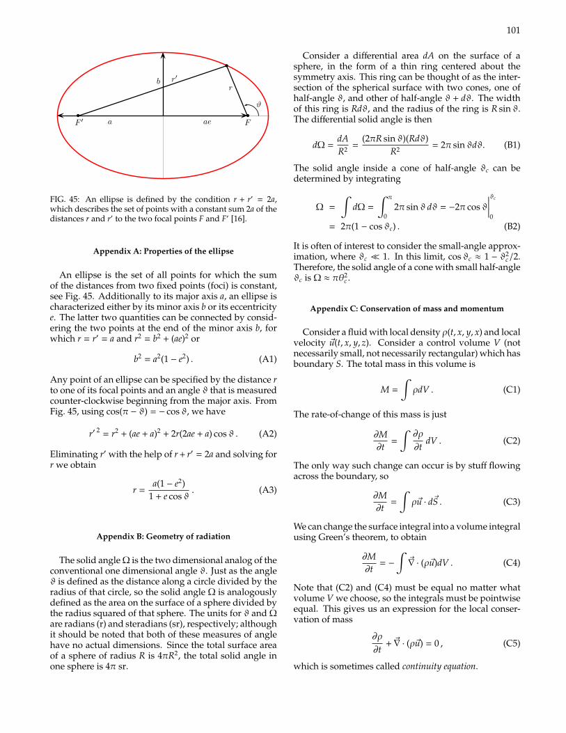
101

5.1 Kepler’s laws

2. The line connecting the Sun and a planet sweeps out equal area in equal time.

3. The “Harmonic Law” states the squared orbital period P of planets measured in yearsequals to the third power of their major axis measured in astronomical units, (P/yr)2 =(a/AU)3.

Kepler noted already that his laws describe also the motion of the Saturn moons, if in theHarmonic Law the appropriate units are used. Newton used later the Harmonic Law to derivethe 1/r2 dependence of the gravitational force. We will follow the opposite way and discusshow Kepler’s laws follow from Newton’s law for gravitation.

Ellipses:An ellipse may be defined by the condition r + r′ = 2a, i.e. as the set of points

with a constant sum 2a of the distances r and r′ to the two focal points F and F ′.Additionally to its major axis a, an ellipse is characterized either by its minor axis bor its eccentricity e. The latter two quantities can be connected by considering thetwo points at the end of the minor axis b: Then r = r′ = a and r2 = b2 + (ae)2 or

b2 = a2(1 − e2) . (5.1)

F ′ F!!

a ae

b r′r

ϑ

!

Any point of an ellipse can be specified by the distance r to one of its focal pointsand an angle ϑ that is measured counter-clockwise beginning from the major axis.From the figure, one obtains immediately (with cos(180 − ϑ) = − cos(ϑ))

r′2 = r2 + (ae + a)2 + 2r(2ae + a) cos ϑ . (5.2)

Eliminating r′ with the help of r + r′ = 2a and solving for r one obtains

r =a(1 − e2)

1 + e cos ϑ. (5.3)

As starting point, we recall how a two-body problem can be reduced to an one-body problemin the case of a central force.

37

FIG. 45: An ellipse is defined by the condition r + r′ = 2a,which describes the set of points with a constant sum 2a of thedistances r and r′ to the two focal points F and F′ [16].

Appendix A: Properties of the ellipse

An ellipse is the set of all points for which the sumof the distances from two fixed points (foci) is constant,see Fig. 45. Additionally to its major axis a, an ellipse ischaracterized either by its minor axis b or its eccentricitye. The latter two quantities can be connected by consid-ering the two points at the end of the minor axis b, forwhich r = r′ = a and r2 = b2 + (ae)2 or

b2 = a2(1 − e2) . (A1)

Any point of an ellipse can be specified by the distance rto one of its focal points and an angle ϑ that is measuredcounter-clockwise beginning from the major axis. FromFig. 45, using cos(π − ϑ) = − cosϑ, we have

r′ 2 = r2 + (ae + a)2 + 2r(2ae + a) cosϑ . (A2)

Eliminating r′ with the help of r + r′ = 2a and solving forr we obtain

r =a(1 − e2)

1 + e cosϑ. (A3)

Appendix B: Geometry of radiation

The solid angle Ω is the two dimensional analog of theconventional one dimensional angle ϑ. Just as the angleϑ is defined as the distance along a circle divided by theradius of that circle, so the solid angle Ω is analogouslydefined as the area on the surface of a sphere divided bythe radius squared of that sphere. The units for ϑ and Ωare radians (r) and steradians (sr), respectively; althoughit should be noted that both of these measures of anglehave no actual dimensions. Since the total surface areaof a sphere of radius R is 4πR2, the total solid angle inone sphere is 4π sr.

Consider a differential area dA on the surface of asphere, in the form of a thin ring centered about thesymmetry axis. This ring can be thought of as the inter-section of the spherical surface with two cones, one ofhalf-angle ϑ, and other of half-angle ϑ + dϑ. The widthof this ring is Rdϑ, and the radius of the ring is R sinϑ.The differential solid angle is then

dΩ =dAR2 =

(2πR sinϑ)(Rdϑ)R2 = 2π sinϑdϑ. (B1)

The solid angle inside a cone of half-angle ϑc can bedetermined by integrating

Ω =

∫dΩ =

∫ π

02π sinϑ dϑ = −2π cosϑ

∣∣∣∣∣ϑc

0

= 2π(1 − cosϑc) . (B2)

It is often of interest to consider the small-angle approx-imation, where ϑc 1. In this limit, cosϑc ≈ 1 − ϑ2

c/2.Therefore, the solid angle of a cone with small half-angleϑc is Ω ≈ πθ2

c .

Appendix C: Conservation of mass and momentum

Consider a fluid with local density ρ(t, x, y, x) and localvelocity ~u(t, x, y, z). Consider a control volume V (notnecessarily small, not necessarily rectangular) which hasboundary S. The total mass in this volume is

M =

∫ρdV . (C1)

The rate-of-change of this mass is just

∂M∂t

=

∫∂ρ

∂tdV . (C2)

The only way such change can occur is by stuff flowingacross the boundary, so

∂M∂t

=

∫ρ~u · d~S . (C3)

We can change the surface integral into a volume integralusing Green’s theorem, to obtain

∂M∂t

= −

∫~∇ · (ρ~u)dV . (C4)

Note that (C2) and (C4) must be equal no matter whatvolume V we choose, so the integrals must be pointwiseequal. This gives us an expression for the local conser-vation of mass

∂ρ

∂t+ ~∇ · (ρ~u) = 0 , (C5)

which is sometimes called continuity equation.

102

We can go through the same process for momentuminstead of mass. We use Π to represent momentum, toavoid conflict with P which represents pressure. Thetotal momentum in the control volume is:

Πi =

∫ρ ui dV , (C6)

where the index i runs over the three components of themomentum. The rate-of-change thereof is just

∂Πi

∂t=

∫∂(ρui)∂t

dV . (C7)

We (temporarily) assume that there are no applied forces(i.e. no gravity) and no pressure (e.g. a fluid of non-interacting dust particles). We also assume viscousforces are negligible. Then, the only way a momentum-change can occur is by momentum flowing across theboundary,

∂Πi

∂t=

∫(ρui)~u · dS =

∫(ρuiu jd jS) . (C8)

We are expressing dot products using the Einstein sum-mation convention, i.e. implied summation over re-peated dummy indices, such as j in the previous expres-sion. We can change the surface integral into a volumeintegral using Green’s theorem, to obtain

∂Πi

∂t= −

∫∇ j(ρuiu j)dV . (C9)

Note that (C7) and (C9) must be equal no matter whatvolume V we choose, so the integrands must be point-wise equal. This gives us an expression for the localconservation of momentum,

∂Πi

∂t=∂(ρui)∂t

= −∇ j(ρuiu j) . (C10)

We can understand this equation as follows: each com-ponent of the momentum-density ρui (for each i sepa-rately) obeys a local conservation law. There are strongparallels between (C5) and (C10). Note that the ∇ j oper-ator on the right-hand-side is differentiating two veloci-ties (ui and u j) only one of which undergoes dot-productsummation (namely summation over j). Using vectorcomponent notation (such as ∇ ju j) is a bit less elegantthan using pure vector notation (such as ~∇ · ~u) but in thiscase it makes things clearer.

We now consider the effect of pressure. It contributesa force on the particles in the control volume, namely

Fi =

∫PdiS = −

∫∇iPdV . (C11)

A uniform gravitational field contributes another force,namely

Fi =

∫ρgidV . (C12)

These forces contribute to changing the momentum, bythe second law of motion:

Π′idt

= Fi . (C13)

Note the tricky notation: we write d/dt rather than ∂/∂t,and Π′ rather than Π, to remind ourselves that the threelaws of motion apply to particles, not to the control vol-ume itself. The rate-of-change of Π, the momentum inthe control volume, contains the Newtonian contribu-tions, (C11) and (C12) via (C13), plus the flow contribu-tions (C10).

Combining all the contributions we obtain the mainresult, Euler’s equation of motion:

∂(ρui)∂t

+ ∇ j(ρuiu j) = −∇iP + ρgi . (C14)

One sometimes encounters other ways of expressingthe same equation of motion. Rather than emphasizingthe momentum, we might want to emphasize the ve-locity. This is not a conserved quantity, but sometimesit is easier to visualize and/or easier to measure. If weexpand the left-hand-side we have

ρ∂ui

∂t+ ui

∂ρ

∂t+ ui∇ j(ρu j) + ρu j∇ jui = ρgi − ∇iP, (C15)

where the second and third terms cancel because of con-servation of mass (C5), leaving us with

ρ∂ui

∂t+ ρu j∇ jui = −∇iP + ρgi . (C16)

Converting from component notation to vector notation,we obtain

ρ∂~u∂t

+ ρ(~u · ~∇

)~u = −~∇P + ρ~g . (C17)

If we now consider a plane-parallel (∂/∂y = 0, ∂/∂z = 0,∂/∂x = d/dx) steady-state (∂/∂t = 0) flow and we ignoregravity, (C5) and (C17) become

ddx

(ρu) = 0 , (C18)

and

ududx

= −1ρ

dPdx

; (C19)

respectively. (C18) immediately gives

ρu = constant→ ρ1u1 = ρ2u2 . (C20)

Using

ddx

(ρu2) = 2ρududx

+ u2 dρdx

= ρududx

+ u(ρ

dudx

+ udρdx

)= ρu

dudx

+ ud

dx(ρu)

= ρududx

(C21)

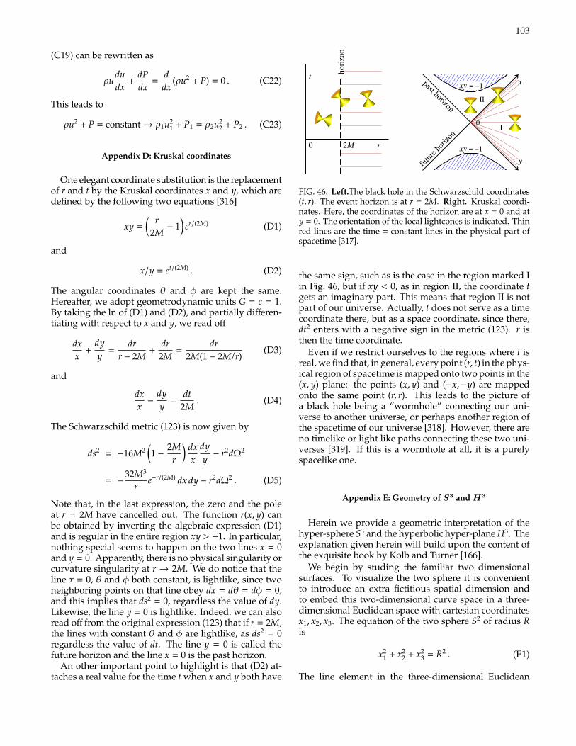
103

(C19) can be rewritten as

ρududx

+dPdx

=ddx

(ρu2 + P) = 0 . (C22)

This leads to

ρu2 + P = constant→ ρ1u21 + P1 = ρ2u2

2 + P2 . (C23)

Appendix D: Kruskal coordinates

One elegant coordinate substitution is the replacementof r and t by the Kruskal coordinates x and y, which aredefined by the following two equations [316]

xy =( r

2M− 1

)er/(2M) (D1)

and

x/y = et/(2M) . (D2)

The angular coordinates θ and φ are kept the same.Hereafter, we adopt geometrodynamic units G = c = 1.By taking the ln of (D1) and (D2), and partially differen-tiating with respect to x and y, we read off

dxx

+dyy

=dr

r − 2M+

dr2M

=dr

2M(1 − 2M/r)(D3)

and

dxx−

dyy

=dt

2M. (D4)

The Schwarzschild metric (123) is now given by

ds2 = −16M2(1 −

2Mr

) dxx

dyy− r2dΩ2

= −32M3

re−r/(2M) dx dy − r2dΩ2 . (D5)

Note that, in the last expression, the zero and the poleat r = 2M have cancelled out. The function r(x, y) canbe obtained by inverting the algebraic expression (D1)and is regular in the entire region xy > −1. In particular,nothing special seems to happen on the two lines x = 0and y = 0. Apparently, there is no physical singularity orcurvature singularity at r → 2M. We do notice that theline x = 0, θ and φ both constant, is lightlike, since twoneighboring points on that line obey dx = dθ = dφ = 0,and this implies that ds2 = 0, regardless the value of dy.Likewise, the line y = 0 is lightlike. Indeed, we can alsoread off from the original expression (123) that if r = 2M,the lines with constant θ and φ are lightlike, as ds2 = 0regardless the value of dt. The line y = 0 is called thefuture horizon and the line x = 0 is the past horizon.

An other important point to highlight is that (D2) at-taches a real value for the time t when x and y both have

0 2M

t

r

horiz

on

y

xxy = −1

future

horiz

on

past horizon

xy = −1

ΙΙ

Ι0

b)a)

Figure 2: a ) The black hole in the Schwarzschild coordinates r, t . The horizonis at r = 2M . b ) Kruskal-Szekeres coordinates; here, the coordinates of thehorizon are at x = 0 and at y = 0 . The orientation of the local lightcones isindicated. Thin red lines are the time = Constant limes in the physical partof space-time.

(6.3) and is regular in the entire region x y > °1 . In particular, nothing special seems tohappen on the two lines x = 0 and y = 0 . Apparently, there is no physical singularityor curvature singularity at r ! 2M . We do notice that the line x = 0, µ and ' bothconstant, is lightlike, since two neighboring points on that line obey dx = dµ = d' = 0 ,and this implies that ds = 0 , regardless the value of dy . similarly, the line y = 0 islightlike. Indeed, we can also read oÆ from the original expression (6.1) that if r = 2M ,the lines with constant µ and ' are lightlike, as ds = 0 regardless the value of dt .The line y = 0 is called the future horizon and the line x = 0 is the past horizon (seeSection 10).

An other important thing to observe is that Eq. (6.4) attaches a real value for thetime t when x and y both have the same sign, such as is the case in the region markedI in Fig. 2 b , but if x y < 0 , as in region II , the coordinate t gets an imaginary part.This means that region II is not part of our universe. Actually, t does not serve as atime coordinate there, but as a space coordinate, since there, dt2 enters with a positivesign in the metric (6.1). r is then the time coordinate.

Even if we restrict ourselves to the regions where t is real, we find that, in general,every point (r, t) in the physical region of space-time is mapped onto two points in the(x, y) plane: the points (x, y) and (°x,°y) are mapped onto the same point (r, r) . Thisleads to the picture of a black hole being a wormhole connecting our universe to anotheruniverse, or perhaps another region of the space-time of our universe. However, there areno timelike or light like paths connecting these two universes. If this is a wormhole at all,it is a purely spacelike one.

12

FIG. 46: Left.The black hole in the Schwarzschild coordinates(t, r). The event horizon is at r = 2M. Right. Kruskal coordi-nates. Here, the coordinates of the horizon are at x = 0 and aty = 0. The orientation of the local lightcones is indicated. Thinred lines are the time = constant lines in the physical part ofspacetime [317].

the same sign, such as is the case in the region marked Iin Fig. 46, but if xy < 0, as in region II, the coordinate tgets an imaginary part. This means that region II is notpart of our universe. Actually, t does not serve as a timecoordinate there, but as a space coordinate, since there,dt2 enters with a negative sign in the metric (123). r isthen the time coordinate.

Even if we restrict ourselves to the regions where t isreal, we find that, in general, every point (r, t) in the phys-ical region of spacetime is mapped onto two points in the(x, y) plane: the points (x, y) and (−x,−y) are mappedonto the same point (r, r). This leads to the picture ofa black hole being a “wormhole” connecting our uni-verse to another universe, or perhaps another region ofthe spacetime of our universe [318]. However, there areno timelike or light like paths connecting these two uni-verses [319]. If this is a wormhole at all, it is a purelyspacelike one.

Appendix E: Geometry of S3 and H3

Herein we provide a geometric interpretation of thehyper-sphere S3 and the hyperbolic hyper-plane H3. Theexplanation given herein will build upon the content ofthe exquisite book by Kolb and Turner [166].

We begin by studing the familiar two dimensionalsurfaces. To visualize the two sphere it is convenientto introduce an extra fictitious spatial dimension andto embed this two-dimensional curve space in a three-dimensional Euclidean space with cartesian coordinatesx1, x2, x3. The equation of the two sphere S2 of radius Ris

x21 + x2

2 + x23 = R2 . (E1)

The line element in the three-dimensional Euclidean

104

space is

ds2 = dx21 + dx2

2 + dx23 . (E2)

If x3 is taken as the fictitious third spatial coordinate, itcan be eliminated from ds2 by the use of (E1)

ds2 = dx21 + dx2

2 +(x1dx1 + x2dx2)2

R2 − x21 − x2

2

. (E3)

Now, introduce the coordinates % and θ defined in termsof x1 and x2 by

x1 = % cosθ and x2 = % sinθ . (E4)

Physically, % andθ correspond to polar coordinates in thex3-plane; x2

3 = R2− %2. In terms of the new coordinates,

(E3) becomes

ds2 =R2d%2

R2 − %2 + %2dθ2 . (E5)

Note the similarity between this metric and the spatialhypersurface with k = 1 in (164).

Another convenient coordinate system for the twosphere is that specified by the usual polar and azimuthalangles (θ, φ) of spherical coordinates, related to xi by

x1 = R sinθ cosφ, x2 = R sinθ sinφ, x3 = R cosθ .(E6)

In terms of these coordinates, (E2) becomes

ds2 = R2[dθ2 + sin2 θdφ

]. (E7)

This form makes manifest the fact that the space is thetwo sphere of radius R.

The equivalent formulas for a space of constant neg-ative curvature can be obtained with the replacementR→ iR in (E1). The metric corresponding to the form of(E5) for the negative curvature case is

ds2 =R2d%2

R2 + %2 + %2dθ2 . (E8)

and the metric in the form corresponding to (E7) is

ds2 = R2[dθ + sinh2 θdφ2

]. (E9)

The embedding of the hyperbolic plane H2 in an Eu-clidean space requires three fictitious extra dimensions,and such an embedding is of little use in visualizing thegeometry. While H2 cannot be globally embedded inR3, it can be partailly represented by the pseudosphere(112).

The generalization of the two-dimensional modelsdiscussed above to three spatial dimensions is trivial.For the three sphere S3 a fictitious fourth spatial di-mension is introduced and in cartesian coordinates thethree sphere is defined by R2 = x2

1 + x22 + x2

3 + x24. The

spatial metric of a four-dimeniosnal Euclidean space isds2 = dx2

1 + dx22 + dx2

3 + dx24. The fictitious coordinate can

be removed to give

ds2 = dx21 + dx2

2 + dx23

+(x1dx1 + x2dx2 + x3dx3)2

R2 − x21 − x2

2 − x23

. (E10)

In terms of coordinates x1 = % sinθ cosφ, x2 =% sinθ sinφ, x3 = % cosθ, the metric is given by thespatial part of (164) with k = 1. In terms of a coor-dinate system that employs the 3 angular coordinates(χ, θ, φ) of a four-dimensional spherical coordinate sys-tem, x1 = R sinχ sinθ cosφ, x2 = R sinχ sinθ sinφ,x3 = R sinχ cosθ, x4 = R cosχ, the metric is given by

ds2 = R2[dχ2 + sin2 χ(dθ2 + sin2 θdφ2)

]. (E11)

The substitution χ = r/R leads to the spatial part of (166)with k = 1.

As in the two-dimensional example, the three-dimensional open model is obtained by the replacementR → iR, which gives the metric in the form (164) withk = −1, or in the form (166) with sinχ → sinhχ. Againthe space is unbounded and R sets the curvature scale.Embedding H3 in an Euclidean space requires four ficti-tious extra dimensions.

Appendix F: Dirac Delta Function

Dirac’s delta function is defined by the following prop-erty

δ(t) =

0 t , 0∞ t = 0

, (F1)

with ∫ t2

t1

dt δ(t) = 1 (F2)

if 0 ∈ [t1, t2] (and zero otherwise). It is “infinitelypeaked” at t = 0, with the total area of unity. You canview this function as a limit of Gaussian

δ(t) = limσ→0

1√

2π σe−t2/(2σ2) , (F3)

or a Lorentzian

δ(t) = limε→0

1π

ε

t2 + ε2 . (F4)

The important property of the delta function is thefollowing relation∫

dt f (t) δ(t) = f (0) , (F5)

105

which is valid for any test function f (t) that is boundedand differentiable to any order, and which vanishes out-side a finite range. This is easy to see. First of all, δ(t)vanishes everywhere except t = 0. Therefore, it does notmatter what values the function f (t) takes except at t = 0.You can then say f (t) δ(t) = f (0) δ(t). Then f (0) can bepulled outside the integral because it does not dependon t, and you obtain the right-hand-side. This equationcan easily be generalized to∫

dt f (t) δ(t − t0) = f (t0) . (F6)

Mathematically, the delta function is not a function,because it is “too singular.” Instead, it is said to be a“distribution.” It is a generalized idea of functions, butcan be used only inside integrals. In fact,

∫dt δ(t) can be

regarded as an “operator” which pulls the value of a testfunction at zero. Put it this way, it sounds perfectly legit-imate and well-defined. But as long as it is understood

that the delta function is eventually integrated, we canuse it as if it is a function.

The step (Heaviside) function,

Θ(x) =

1 x ≥ 00 x < 0

, (F7)

is the “primitive” (at least in symbolyc form) of the δ(x).Equivalently, Θ′(x), has the symbolic limit δ(x), as weshow next. For any given test function f (x), integrationby parts leads to∫ +∞

−∞

Θ′(x) f (x)dx = −

∫ +∞

−∞

Θ(x) f ′(x)dx

= −

∫∞

0f ′(x)dx = f (0) ; (F8)

therefore Θ′(x) = δ(x).