lectures on linear and nonlinear dispersive waves draft...

Lectures on Linear and Nonlinear Dispersive Waves

DRAFT IN PROGRESS

M.I. Weinstein ∗

October 22, 2006

Contents

1 Some Basic Analysis 31.1 Function spaces . . . . . . . . . . . . . . . . . . . . . . . . . . . . . . . . . . 31.2 Linear operators . . . . . . . . . . . . . . . . . . . . . . . . . . . . . . . . . . 31.3 Fourier Transform . . . . . . . . . . . . . . . . . . . . . . . . . . . . . . . . . 31.4 Fourier inversion on S and L2 . . . . . . . . . . . . . . . . . . . . . . . . . . 41.5 Sobolev spaces on IRn . . . . . . . . . . . . . . . . . . . . . . . . . . . . . . 51.6 Notes and references for section 1 . . . . . . . . . . . . . . . . . . . . . . . . 6

2 Linear dispersive PDEs - introduction 62.1 Dispersion relations, examples . . . . . . . . . . . . . . . . . . . . . . . . . . 6

3 Introduction to the Schrodinger equation 83.1 Quantum mechanics . . . . . . . . . . . . . . . . . . . . . . . . . . . . . . . 83.2 Free Schrodinger - initial value problem . . . . . . . . . . . . . . . . . . . . . 83.3 Free Schrodinger in Lp . . . . . . . . . . . . . . . . . . . . . . . . . . . . . . 93.4 Structural properties of the Schrodinger equation . . . . . . . . . . . . . . . 103.5 Free evolution of a Gaussian wave packet . . . . . . . . . . . . . . . . . . . . 113.6 Observables . . . . . . . . . . . . . . . . . . . . . . . . . . . . . . . . . . . . 123.7 The Uncertainty Principle . . . . . . . . . . . . . . . . . . . . . . . . . . . . 12

4 Oscillatory integrals and Dispersive PDEs 134.1 Non-stationary phase . . . . . . . . . . . . . . . . . . . . . . . . . . . . . . . 144.2 Stationary Phase . . . . . . . . . . . . . . . . . . . . . . . . . . . . . . . . . 154.3 Degenerate dispersion and Van der Corput’s Lemma . . . . . . . . . . . . . . 174.4 PDE asymptotics via localization in Fourier space . . . . . . . . . . . . . . . 204.5 Notes and references for Section 4 . . . . . . . . . . . . . . . . . . . . . . . . 20

∗Department of Applied Physics and Applied Mathematics, Columbia University, New York, NY 10027

1

CONTENTS DRAFT: October 22, 2006

5 The Nonlinear Schrodinger / Gross-Pitaevskii Equation 205.1 “Universality” of NLS . . . . . . . . . . . . . . . . . . . . . . . . . . . . . . 215.2 Multiple scales . . . . . . . . . . . . . . . . . . . . . . . . . . . . . . . . . . 215.3 Hierarchy of equations . . . . . . . . . . . . . . . . . . . . . . . . . . . . . . 225.4 Solution of equation hierarchy . . . . . . . . . . . . . . . . . . . . . . . . . . 235.5 Conclusion and Theorem . . . . . . . . . . . . . . . . . . . . . . . . . . . . . 24

6 Structural Properties of NLS 246.1 Hamiltonian structure . . . . . . . . . . . . . . . . . . . . . . . . . . . . . . 246.2 Symmetries and conserved integrals . . . . . . . . . . . . . . . . . . . . . . . 24

7 Formulation in H1 and the basic well-posedness theorem 24

8 Special solutions of NLS - nonlinear plane waves and nonlinear boundstates 24

9 Appendices 259.1 The M. Riesz Convexity Theorem . . . . . . . . . . . . . . . . . . . . . . . . 259.2 The Implicit Function Theorem . . . . . . . . . . . . . . . . . . . . . . . . . 259.3 The Contraction Mapping Principle . . . . . . . . . . . . . . . . . . . . . . . 25

2

DRAFT: October 22, 2006

1 Some Basic Analysis

1.1 Function spaces

Definition 1.1 Schwartz class, S(IRn), is the vector space of functions which are C∞ andwhich, together with all their derivatives, decay faster than any polynomial rate. Specifically,if f ∈ S, then for any α, β ∈ Nn

0 , there exists a constant Cα,β such that

supx∈IRn

|xα∂βxf(x)| ≤ Cα,β

Lp(IRn) spaces, 1 ≤ p ≤ ∞S is dense in Lp

Theorem 1.1 (Approximation of the identity) Let K(x) > 0 and∫K(x)dx = 1. Define

KN(x) = NnK(Nx), N ≥ 1.Let f be a bounded and continuous function on IRn and consider the convolution

KN ⋆ f(x) =

∫KN (x− y) f(y) dy (1.1)

Then, KN ⋆ f(x) → f(x) uniformly on any compact subset, C, of IRn as N ↑ ∞, i.e.maxx∈C | [KN ⋆ f ](x) − f(x)| → 0.

1.2 Linear operators

Definition 1.2 A linear transformation, T , between vector spaces X1 and X2...

Definition 1.3 A bounded linear transformation...

Example 1.1 Symmetric matrix n by n

Theorem 1.2 Let T : E → Y be a BLT.

1.3 Fourier Transform

For f ∈ S define the Fourier transform, f or Ff by

f(ξ) = Ff(ξ) =

∫e−2πix·ξf(x) dx (1.2)

Proposition 1.1 Assume f ∈ S.

(a) f ∈ C∞ and ∂β f(ξ) =[

(−2πix)βf(x)]

(ξ)

(b) ∂βf(ξ) = (2πiξ)β f(ξ)

(c) f ∈ S. Thus, the Fourier transform maps S to S.

3

1.4 Fourier inversion on S and L2 DRAFT: October 22, 2006

Theorem 1.3 Riemann-Lebesgue Lemmaf ∈ L1(IRn) =⇒ limξ→∞ f(ξ) = 0.

Proof: Approximate by step functions, for which the result can be checked. Note: no rateof decay of the Fourier transform is implied by f ∈ L1.

Theorem 1.4 Let f(x) ≡ e−πa|x|2. Then,

f(ξ) = a−n2 e−π

|ξ|2

a (1.3)

Proof: Write out definition of f . Note that the computation factors into computing theFourier transform of n independent one dimensional Gaussians. For the one-dimensionalGaussian, complete the square in the exponent, deform the contour using analyticity of theintegrand, and finally use that

∫IR e

−πy2dy = 1.

1.4 Fourier inversion on S and L2

Definition: For g ∈ S define g

g(x) ≡∫e2πiξ·xg(ξ) dξ = g(−x)

Proposition 1.2 ∫f g dx =

∫f g dx (1.4)

Proof: Interchange orders of integration (Fubini’s Theorem).

Theorem 1.5 Fourier inversion formula Assume f ∈ S. Then,

f ∈ S =⇒ g(x) = f(x), where g(ξ) = f(ξ) (1.5)

Proof: We shall prove Fourier inversion in the following sense.

limε→0

∫e−πε2|ξ|2 e2πix·ξ f(ξ) dξ = f(x)

For any ε > 0 defineφε(ξ) = e2πix·ξ − πε2|ξ|2

whose Fourier transform is

φε(y) =1

εne−π |x−y|2

ε2 =1

εng

(x− y

ε

)≡ gε(x− y)

4

1.5 Sobolev spaces on IRn DRAFT: October 22, 2006

Now,

∫e−πε2|ξ|2 e2πix·ξ f(ξ) dξ =

∫φε(ξ) f(ξ) dξ

=

∫φε(y) f(y) dy

=

∫gε(x− y) f(y) dy → f(x)

as ε ↓ 0 because gε is an approximation of the identity; see Theorem 1.1

Theorem 1.6 (Plancherel Theorem) Assume f ∈ S. Then,

‖f‖2 = ‖f‖2

Therefore, the Fourier transform preserves the L2 norm on S. Furthermore, for any f, g ∈ S∫f g dx =

∫F [f ] F [g]

Corollary 1.1 The Fourier transform can be extended to a unitary operator defined on allL2 such ‖f‖2 = ‖f‖2.

Proof: A BLT argument. S is dense in L2. If f ∈ L2, there exists a sequence fj ∈ S such

that ‖fj − f‖2 → 0. Define f = limj→∞ fj .

1.5 Sobolev spaces on IRn

Definition 1.4 (1) For any s ∈ IR, define the Hs(IRn) norm for u ∈ S(IRn) by

‖u‖2Hs =

∫|u(ξ)|2 (1 + |ξ|2)s dξ. (1.6)

(2) The Sobelev space Hs = Hs(IRn) is defined to be the completion of S(IRn) with respectto the norm ‖ · ‖Hs.

The following estimate shows the important connection between the control of derivativesof a function in L2 with the pointwise behavior of a function.

Theorem 1.7 (Sobelev Lemma) Let k be a non-negative integer. Let u ∈ Hs(IRn), wheres > k + n/2. Then, u is almost everywhere (in the measure theoretic sense) equal to afunction of class Ck. Moreover, for any α ∈ Nn with |α| = k, we have ∂αu ∈ C↓(IR

n) andthere exists a constant C > 0 depending only on s, α, n, but not on u, such that

‖∂αu‖L∞ ≤ C ‖u‖Hs.

5

1.6 Notes and references for section 1 DRAFT: October 22, 2006

The connection between the general Lq behavior of a function and that of its Sobelevspace regularity also plays an important role, quite often in nonlinear problems. We will usethe following special case of the Sobelev-Nirenberg-Gagliardo estimate:

Theorem 1.8 Let f be in H1. Then, f is almost everywhere equal to an Lq function for2 ≤ q < 2q

n−2if n ≥ 3 and all q ≥ 2 if n = 1 or n = 2. Furthermore,

‖ f ‖Lq ≤ Cq,n ‖f‖H1, and in fact

‖ f ‖Lq ≤ Cq,n ‖∇f‖n q−22q

L2 ‖f‖1−n q−22q

L2 (1.7)

1.6 Notes and references for section 1

A good short and user-friendly introduction to basic functional analysis appears in Chapter0 of G.B. Folland’s text on PDEs [1]. Volume 1 of Reed-Simon’s series, Functional Analysis[3], contains a discussion, going considerably further.

2 Linear dispersive PDEs - introduction

In this section we introduce the notion of dispersion and give numerous examples. A goodreference is [6].

2.1 Dispersion relations, examples

Consider a system of m linear, constant coefficient, homogeneous partial differential equa-tions:

P (i∂t,−i∂x1 , . . . ,−i∂xn)u(x, t) = 0 (2.1)

Here, for simplicity, we take P (τ, k1, . . . , kn) to be an n by m matrix, whose entries arepolynomials in τ and ξk. A plane wave solution is a solution of the form ei(k·x−ωt)w, where wis a constant vector in IRn. Substitution into (2.1) yields the system of algebraic equationsfor v:

P (ω, k1, . . . , kn) w = 0

A non-trivial plane wave solution exists if and only if

G(ω, k) ≡ detP (ω, k) = 0. (2.2)

The relation (2.2) is called the dispersion relation of the system of PDEs. We assume itdefines m real-valued branches of the form

ω = ω(k), for which G(ω(k), k) = 0 (2.3)

Example 2.1 Transport equation

∂tu+ v · ∇u = 0 (2.4)

Dispersion relation: ω(k) = v · k.

6

2.1 Dispersion relations, examples DRAFT: October 22, 2006

Example 2.2 One dimensional wave equation

c−2∂2t u = ∂2

xu (2.5)

Dispersion relation: c−2ω2(k)− k2 = 0, defining two branches ω+(k) = ck and ω−(k) = −ck.

Example 2.3 One dimensional Klein-Gordon equation

c−2∂2t u =

(∂2

x − m2)u, m > 0. (2.6)

Dispersion relation: c−2ω2(k) − (m2 + k2) = 0, defining two branches ω+(k) = c√m2 + k2

and ω−(k) = −c√m2 + k2.

Example 2.4 Free Schrodinger equation

i~∂t ψ = − ~2

2m∆ψ (2.7)

Dispersion relation: ω(k) = ~

2m|k|2

Example 2.5 One dimensional beam equation

∂2t u + γ2∂4

xu. (2.8)

Dispersion relation: ω+(k) = γk2 and ω−(k) = −γk2.

Exercise 2.1 Show that if ψ = U+iV , where U and V are real, satisfies the free Schrodingerequation, then U and V each statisfy the beam equation.

Example 2.6 Linearized KdV aka Airy equation

∂tu + c∂xu + ∂3xu = 0. (2.9)

Dispersion relation: ω(k) = ck − k3.

Example 2.7 Linearized BBM

∂tu + c∂xu − ∂2x∂tu = 0. (2.10)

Dispersion relation: ω(k) = ck1+k2 .

Example 2.8 Coupled mode equations

∂tE+ + ∂xE+ + κE− = 0

∂tE− + ∂xE− + κE+ = 0 (2.11)

Dispersion relation: ω±(k) = ±√κ2 + k2. Note that the first order system (2.11) has the

same dispersion relation as the Klein-Gordon equation (2.6), with κ = m.

7


3 Introduction to the Schrodinger equation

In this section we introduce the Schrodinger equation in two ways. First, we mention howit arises in the fundamental description of quantum atomic phenomena. We then show itsrole in the description of diffraction of classical waves.

3.1 Quantum mechanics

The hydrogen atom: one proton and one electron of mass m and charge e. The state of theatom is given by a function ψ(x, t), complex-valued, defined for all x ∈ IR3 and t ∈ IR. ψ isoften called the wave function.Let Ω ⊂ IR3. |ψ(x, t)|2 dx is a probability measure with the interpretation

∫

D

|ψ(x, t)|2 dx = Probability (electron ∈ Ω at time t)

Thus, we require

∫

IR3|ψ(x, t)|2 dx = Probability

(electron ∈ IR3 at time t

)= 1

Given an initial wave function, ψ0

i~ ∂tψ = H ψ

H = − ~2

2m∆ + V (x) (3.1)

Here, ~ denotes Planck’s constant divided by 2π. The operator H is called a Schrodingeroperator with potential V , a real-valued function determined by the nucleus. For the specialcase of the hydrogen atom

H = − ~2

2m∆ − e2

r, r = |x| (3.2)

The free electron (unbound to any nucleus) is governed by the free Schrodinger equation(V ≡ 0):

i~ ∂tψ = − ~2

2m∆ψ (3.3)

3.2 Free Schrodinger - initial value problem

Initial Value Problemi∂tu = −∆ u, u(x, 0) = f(x) (3.4)

Unlike the heat equation, ∂tu = ∆u, which has an exponentially decaying Gaussian fun-damental solution, the fundamental solution of the Schrodinger equation is an oscillatoryGaussian with no spatial decay. For this reason, the derivation of the solution to the initial

8

3.3 Free Schrodinger in Lp DRAFT: October 22, 2006

value problem is more subtle. One approach is to regularize the Schrodinger equation byadding a small (ε > 0) diffusive term, which we then take to zero (ε→ 0).

Regularized initial value problem Take ε > 0.

i∂tuε = −(1 − iε)∆ uε, uε(x, 0) = f(x) (3.5)

Lemma 3.1f(x) = e−πa|x|2, ℜa ≥ 0 =⇒ f(ξ) = a−

n2 e−

πa|ξ|2 (3.6)

Solution of regularized IVP

i∂tuε = 4π2(1 − iε)|ξ|2u

uε(ξ, t) = e−4π2(i+ε)|ξ|2t f(ξ) (3.7)

uε(x, t) =

∫Kε

t (x− y) f(y) dy,

where

Kεt (x) =

∫e−2πix·ξ e−4π2(i+ε)|ξ|2t dξ. (3.8)

Here, we have used that for ε > 0, e2πiξ·(x−y) e−4π2(i+ε)|ξ|2t f(y) ∈ L1(dξdy), so we caninterchange integrals by Fubini’s Theorem.

We now apply Lemma 3.1 with a = (4π(i+ ε)−1 and obtain

Kεt (x) = (4π(i+ ε)t)−n/2 e−

|x|2

4t(i+ε)

For any t 6= 0, if f ∈ L1, we can pass to the limit ε → 0+ by the Lebesgue dominatedconvergence theorem. We define the free Schrodinger evolution by

u(x, t) = ei∆tf =

∫Kt(x− y) f(y) dy

Kt(x) = (4πit)−n/2 ei |x|2

4t , (3.9)

where (3.9) is understood as limε→0+ Kεt ⋆ f .

For f ∈ L2, we can use that the Fourier transform is defined (and unitary) on all L2 todefine, by (3.7),

u(x, t) =(e−4π2i|ξ|2t f(ξ)

)(x, t) = ei∆tf (3.10)

3.3 Free Schrodinger in Lp

ei∆tf for f ∈ L1(IRn): In this case,

|u(x, t)| =

∣∣∣∣∫

Kt(x− y) f(y) dy

∣∣∣∣ ≤∫

|f | dy

9

3.4 Structural properties of the Schrodinger equation DRAFT: October 22, 2006

Therefore, if f ∈ L1(IRn), then ei∆tf ∈ L∞(IRn) for t 6= 0 and

‖ ei∆tf ‖L∞ ≤ |4πt|−n2 | ‖f‖L1 (3.11)

ei∆tf for f ∈ L2(IRn): In this case

∫|u(x, t)|2dx =

∫|u(ξ, t)|2dξ =

∫|e−4π2i|ξ|2t f(ξ)|2dξ =

∫|f(ξ)|2dξ

Thus, if f ∈ L2(IRn), then ei∆tf ∈ L2(IRn) and

‖ei∆tf‖L2 = ‖f‖L2 (3.12)

Extension to Lp: Suppose f ∈ Lp(IRn) with 1 ≤ p ≤ 2. Using a theorem of M. Riesz oninterpolation of linear operators, Theorem 9.1, one can show:

Theorem 3.1 Let 1 ≤ p ≤ 2 and 2 ≤ q ≤ ∞, where p−1 + q−1 = 1. If f ∈ Lp(IRn), thenfor t 6= 0 ei∆tf ∈ Lq(IRn) and

‖ei∆tf‖Lq ≤ |4πt|−(n2−n

q) ‖f‖Lp (3.13)

3.4 Structural properties of the Schrodinger equation

Invariances properties: The following transformations map solutions of the free Schrodingerequation to solutions of free Schrodinger equation.

(1) Spatial translation: u(x, t) 7→ u(x+ x0, t), x0 ∈ IRn

(2) Time translation: u(x, t) 7→ u(x, t+ t0), t0 ∈ IR

(3) Complex conjugation: u(x, t) 7→ ¯u(x, t)

(4) Time-reversal / conjugation: u(x, t) 7→ u(x,−t)

(5) Galilean invariance:

u(x, t) 7→ Gη[u](x, t) = eiη·(x−ηt) u(x− 2ηt, t). (3.14)

Remark 3.1 Note that (3.14) contains the two velocities: vphase(η) = ω(η)/η = η andvgroup(η) = 2η, the group velocity. Energy propagates with the group velocity; see Remark3.2.

10

3.5 Free evolution of a Gaussian wave packet DRAFT: October 22, 2006

3.5 Free evolution of a Gaussian wave packet

Consider the evolution of a Gaussian wave-packet in one-space dimension. Let η0 = 2πξ0.

i∂tu = −∂2xu

u(x, 0) = eiη0x e−x2

2L2 = gL,η0(x) (3.15)

Thus u(x, 0) is an oscillatory and localized initial condition with carrier oscillation periodξ−10 or frequency ξ0. Its evolution has an elegant and illustrative form:

Theorem 3.2

u(x, t) = ei∆tgL,η0 =eiη0(x−η0t)

(1 + 2it

L2

) 12

e−

(x−2η0t)2

2L2(1+ 2itL2 ) (3.16)

Proof of Theorem 3.2 : The Fourier representation of the solution is:

u(x, t) =

∫e2πiξxgL,2πξ0(ξ) dξ (3.17)

Note: gL,2πξ0(ξ) = gL,0(ξ−ξ0) = (2π)12 L e−2π2L2(ξ−ξ0)2 . Substitution into (3.17) and grinding

away with such tools as completing the square yields the result.

A “better” proof of Theorem 3.2: We prove the result in two steps. Step 1: Treat thecase where η0 = 0, u(x, 0) = gL,0. Step 2: Apply the Galilean transformation, Gη0 , to obtainTheorem for general η0.Step 1: u(t) = ei∆tgL,0 is the convolution of Gaussians. Thus, it is useful to have

Lemma 3.2 Let Ga(x) = e−aπ|x|2. Let a and b be such that ℜa ≥ 0, ℜb ≥ 0, a 6= 0 andb 6= 0. Then,

Ga ⋆ Gb =1

(a + b)n2

G aba+b

(3.18)

Proof of Lemma 3.2: The Fourier transform of the right hand side of (3.18) is the productof the Fourier transforms, computed using Theorem 1.3. Rewriting this product as a singleGaussian and computing the inverse transform, using Theorem 1.3, gives the result.Step 2: Note that the Galilean boost: U(x, t) = Gη0 [e

i∆tgL,0] solves the initial value problemfor the free Schrodinger equation with initial data U(x, 0) = eiη0xgL,0, as desired. This givesthe formula (3.16).

Remark 3.2 • Phase propagates with velocity η0, the phase velocity

• Energy ∼ |u(x, t)|2 propagates with velocity 2η0, the group velocity

• Solution disperses (spreads and decays) to zero as t ↑. This is seen from the generalestimate (3.11) as well as the explicit solution (3.16).

• However, solution does not decay in L2. The Schrodinger evolution is unitary in L2;see (3.12).

• Concentrated (sharp) initial conditions (L small) disperse more quickly than spread outinitial conditions (L large). The time scale of spreading is t ∼ L2.

11

3.6 Observables DRAFT: October 22, 2006

3.6 Observables

Recall that |ψ(x, t)|2 has the interpretation of a probability density for a quantum particleto be at position x at time t. |ψ(ξ, t)|2 has the interpretation of a probability density for aquantum particle to be at momentum ξ at time t.

The expected value of an observable or operator , A, is formally given by1

〈A〉 = (ψ,Aψ) =

∫ψAψ (3.19)

Theorem 3.3d

dt〈A〉 = i〈[H,A]〉, (3.20)

where [B,A] = BA− AB.

Examples

(i) 〈X〉, the average position =∫x|ψ(x, t)|2dx.

(ii) 〈Ξ〉 =∫ξ|ψ(ξ, t)|2dξ; Let Pk = −i∂xk

, the momentum operator. Then, 〈Pk〉 =2π〈Ξ〉 is the average momentum.

(iii) 〈|X|2〉, the variance or uncertainty in position =∫|x|2|ψ(ξ, t)|2dx.

(iv) 〈|Ξ|2〉, the variance or uncertainty in momentum =∫|ξ|2|ψ(ξ, t)|2dξ.

Exercise 3.1 Show that 〈Xk〉(t) = 〈Xk〉(0) + 2〈Pk〉(0) t.

3.7 The Uncertainty Principle

Theorem 3.4 (Uncertainty Inequality) Suppose xf and ∇f are in L2(IRn). Then,

∫|f |2 ≤ 2

n

(∫|xf |2

) 12(∫

|∇f |2) 1

2

or equivalently ∫|f |2 ≤ 4π

n

(∫|xf |2

) 12(∫

|ξf |2) 1

2

(3.21)

Exercise 3.2 (a) Prove the uncertainty inequality, using the pointwise identity

x · ∇|f |2 = ∇ · (x|f |2) − n |f |2,

(b) Prove that the inequality (3.21) is sharp in the sense that equality is attained for theGaussian f(x) = exp(−|x|2/2).

1We proceed formally, without any serious attention to operator domains etc. For a fully rigorous treat-ment, see [3].

12


Applying the uncertainty inequality (3.21) to a solution of the Schrodinger equation, withinitial condition ‖ψ(·, 0)‖L2 = 1 and we have,

1 =

∫|ψ(x, 0)|2dx =

∫|ψ(x, t)|2dx ≤ 4π

n

(∫|xψ(x, t)|2

) 12(∫

|ξψ(ξ, t)|2) 1

2

(3.22)

The latter, can be written as

n

4π≤√〈|X|2〉(t)

√〈|Ξ|2〉(t) (3.23)

and is called Heisenberg’s uncertainty principle.

4 Oscillatory integrals and Dispersive PDEs

Consider a scalar constant coefficient partial differential equation

∂tu = P (D) u, D = (∂x1 , . . . , ∂xn) (4.1)

Assuming a real-valued dispersion relation ω = ω(k), we have that the solution to the initialvalue problem with initial data u(x, 0) = g(x) has the form

u(x, t) =

∫ei(x·ξ−ω(ξ)t) g(ξ) dξ (4.2)

Question: What is the large time (t→ ∞) behavior of u(x, t)?This question is now considered in the context of the following more general question in theasymptotic analysis of oscillatory integrals of the form

I(λ) =

∫eiλφ(ξ) h(ξ) dξ, for λ→ ∞ (4.3)

where φ(ξ) is a smooth and real-valued a phase-function.Our goal in this section is to make precise the notion that: as λ→ ∞, rapid oscillations

of eiλφ(ξ) tend to cancel each other out and the dominant contribution from I(λ) comes froma neighborhood of points, ξ, for which ∇φ(ξ) = 0.

Here’s the idea; when in doubt, integrate by parts. Let’s consider the integral:∫ b

aeiλφ(ξ)dξ.

If φ′ 6= 0 on [a, b], then

∫ b

a

eiλφ(ξ)dξ =

∫ b

a

1

iλφ′(ξ)

d

dξeiλφ(ξ)dξ

=1

iλφ′(ξ)eiλφ(ξ)

∣∣∣ξ=bξ=a −

∫ b

a

eiλφ(s) d

ds

1

iλφ′(s)ds

13

4.1 Non-stationary phase DRAFT: October 22, 2006

Therefore, |∫ b

aeiλφ(ξ)dξ| ≤ C|λ|−1 maxa≤ξ≤b |φ′(ξ)|−1. If there is an interior point ξ0, a <

ξ0 < b, at which φ′(ξ0) = 0 and φ′′(ξ0) 6= 0. Then, we break the integral into an integralover a small neighborhood of ξ0 (or, more generally, neighborhoods of any finite set of non-degenerate critical points of φ,) and an integral over the complement of this neighborhood.On the complement, φ′ 6= 0 so the previous estimate holds. On the small neighborhood ofξ0, we have φ(ξ) ∼ φ(0)+ 1

2φ′′(ξ0)(ξ− ξ0)2. Therefore, the contribution from a neighborhood

of ξ0 comes from a Gaussian integral, which can be estimated as O(

(|φ′′(ξ0)| |λ|)−12

). We

now proceed with a rigorous treatment.

4.1 Non-stationary phase

Theorem 4.1 (Non-stationary phase) Let K be a compact subset of IRn. Suppose φ is real-valued and defined on a neighborhood, O, of K, such that φ ∈ Cr+1(O) and such that ∇φ 6= 0on K. Let h ∈ Cr

0(int(K)). Then,

| I(λ) | ≤ C〈λ〉−r ‖h‖r,∞, (4.4)

where‖u‖r,∞ =

∑

|α|≤r

‖∂αu‖∞, (4.5)

C = C (maxK |∇ξφ|−1, ‖∂φ‖r,∞) and C(s, s′) → ∞ as s or s′ tend to infinity. In particular,if φ and h are C∞ then I(λ) = O(〈λ〉−r) for any r > 0.

Proof of Theorem 4.1: First note that for |λ| ≤ 1 we can use the bound | I(λ) | ≤ ‖h‖L1 .Therefore, it suffices to consider |λ| ≥ 1.

We seek an operator L =∑n

j=1 bj(ξ)∂ξj

such that

L eiλφ(ξ) = eiλφ(ξ)

In order to see how to choose bj , compute:

L eiλφ(ξ) = eiλφ(ξ)

(n∑

j=1

iλ ∂ξjφ(ξ) bj(ξ)

)

implying the choice

bj(ξ) =1

iλ|∇φ(ξ)|−2 ∂ξj

φ(ξ) (4.6)

Note that if h has compact support then,

I(λ) =

∫eiλφ(ξ) h(ξ) dξ

=

∫Lr(eiλφ(ξ)) h(ξ) dξ

=

∫eiλφ(ξ) (Lt)r h(ξ) dξ,

(4.7)

14

4.2 Stationary Phase DRAFT: October 22, 2006

where

Lt = − 1

iλ

n∑

j=1

∂ξj

(|∇φ(ξ)|−2 ·

)(4.8)

Since |eiλφ| = 1, we have

| I(λ) | ≤∫

| (Lt)r h(ξ) | dξ.

Note that (Lt)r contains a factor λ−r. The proof now follows by expanding and estimatingthe right hand side.

Corollary 4.1 Let g(ξ), appearing in the expression for u(x, t) in (4.2), be smooth and havecompact support. Denote by

Λ = ∇ξ ω(ξ) : ξ ∈ supp(g) (4.9)

Let G ⊂ IRn be an open subset which contains Λ. For any m = 1, 2, . . . , there exists aconstant c = c(m, g,G), such that for any (x, t) with x/t /∈ G:

|u(x, t)| ≤ c〈|t| + |x|〉−m (4.10)

4.2 Stationary Phase

Theorem 4.2 (Stationary Phase) Let φ, defined in a neighborhood of the origin 0 ∈ IRn,be a C∞ and real-valued function. Assume that 0 is a non-degenerate critical point of φ, i.e.∇φ(0) = 0 and Hφ(0) = ( φξiξj

(0) ) is invertible. Then, there exist neighborhoods O and O′

of the origin and a constant C > 0, such that for all h ∈ C∞0 (O)

| I(λ) | ≤ C | detHφ(0) |−n2 〈λ〉−n

2 ‖h‖Hs , s >n

2(4.11)

Corollary 4.2 Consider u(x, t), given by (4.2), where g ∈ C∞0 and

supp(g) ∩ ξ : det(φξiξj)(0) = 0 is empty.

Then, for all x, t|u(x, t)| ≤ C | detHφ(0)|−n

2 〈t〉−n2 (4.12)

The proof of the stationary phase theorem uses the following

Lemma 4.1 (Morse Lemma)Let φ satisfy the hypotheses of Theorem 4.2. In particular, ∇φ(0) = 0 and Hφ(0) =

( φxj ,xk(0) ) is non-singular. There exist open neighborhoods O and O′ of the origin and a

C∞ invertible mapping X : O → O′, such that

X(k) = k + O(|k|2)

φ(k) = φ(0) +1

2(X(k), AX(k)) . (4.13)

for k ∈ O, where here (a, b) = aT b.

15

4.2 Stationary Phase DRAFT: October 22, 2006

Proof of the Morse Lemma: As in the proof of Taylor’s Theorem, we have

φ(k) − φ(0) =

∫ 1

0

d

dtφ(tk) dt

= (t− 1)d

dtφ(tk)

∣∣t0 −

∫ t

0

(t− 1)d2

dt2φ(tk) dt

=

(k,

∫ 1

0

(1 − t) Hφ(tk) dt k

)

≡ 1

2(k,B(k)k), where (4.14)

Bij(k) = 2

∫ 1

0

φkikj(sk) (1 − s) ds (4.15)

We seek a C∞ n by n matrix R(k), such that R∗(k)AR(k) = B(k). If we can find such amatrix, R(k), with R(k) = I + O(|k|), then

(k,B(k)k) = (k,R∗(k)AR(k)k) = ([R(k)k], A[R(k)k])

and defining X(k) = R(k)k does the trick.We construct R(k) by applying the implicit function theorem to the matrix equation

F (R,B) ≡ R∗(k)AR(k) − B(k) = 0, (4.16)

in a neighborhood of the solution R = I, B = A.Here’s the setup. Let

(i) M = the vector space of all n by n matrices.

(ii) Ms = the vector space of all n by n symmetric matrices.

Then, the mapping F : (R,B) 7→ F (R,B) maps M ×Ms → Ms, by the symmetry of A. Wealso have F (I, A) = 0. To apply the implicit function theorem in a neighborhood of (I, A),we first compute the Jacobian FR(R,B) evaluated at (R,B) = (I, A).

Computation of FR(R,B):

F (R + ǫC,B) − F (R,B) = (R∗ + ǫC∗)A(R + ǫC) − R∗AR

= R∗AR + ǫ(C∗AR + R∗AC) + O(ǫ2) (4.17)

Thus,

FR(R,B) C = C∗AR + R∗AC, and therefore

FR(I, A) C ≡ T (C) = C∗A + AC (4.18)

To apply the implicit function theorem, we need to check that T : M →Ms is one to oneand onto.

(a) T is one to one. Proof: Exercise

16

4.3 Degenerate dispersion and Van der Corput’s Lemma DRAFT: October 22, 2006

(b) T is onto: Let D ∈ Ms. We need to show that C∗A + AC = D has a solution. LetC = 1

2A−1D, which exists because A is assumed invertible. Then one can easily check

that T (C) = D.

By the implicit function theorem, there exists an neighborhood A ⊂Ms of A and a C∞ mapR : A → M , such that F (R(A), A) = 0, R(A) = I. Now choose O, an open neighborhoodof k = 0, so that k ∈ O implies that B(k) ∈ A, and take X(k) = R(B(k))k. This completesthe proof.

Proof of Stationary Phase Theorem: Consider the integral

I(λ) =

∫eiλφ(ξ) h(ξ) dξ.

By the Morse Lemma, in a sufficiently small neighborhood, O, of ξ = 0 we have

φ(ξ) = φ(0) +1

2〈X(ξ), AX(ξ)〉, where A = Hφ(0) (4.19)

is the Hessian matrix of φ(ξ) at the critical point ξ = 0. Assume that h is supported withinO. Then,

I(λ) = eiλφ(0)

∫eiλ〈X(ξ),AX(ξ)〉/2 h(ξ) dξ

Set y = X(ξ). Then,

I(λ) = eiλφ(0)

∫eiλ〈y,Ay〉/2 (h X−1)(y)

∣∣detDξX(X−1(y))|∣∣−1

dy

= eiλφ(0)

∫v(y) e−iλ〈y,Ay〉/2 dy, where

v(y) = (h X−1)(y)∣∣detDξX(X−1(y))|

∣∣−1

By the Plancherel Theorem 1.6,

| I(λ) | =

∣∣∣∣∫

Fv(η) Fe−i λ〈y,Ay〉2 (η) dη

∣∣∣∣

≤ C | det(A)λ|−n2

∫|Fv(η)| dη

≤ C ′ | det(A)λ|−n2 ‖v‖Hs

≤ C ′′ | det(Hφ(0)) λ|−n2 ‖h‖Hs, s > n/2 (4.20)

4.3 Degenerate dispersion and Van der Corput’s Lemma

It may happen that the oscillatory integral, I(λ), has points of stationary phase, which aredegenerate. We consider an example:Airy / linearized KdV:For concreteness, consider the initial value problem for the linearized KdV (Airy equation);see Example 2.6:

∂tu + ∂3xu = 0, u(x, 0) = g(x) (4.21)

17


The dispersion relation, as noted in section 2, is ω(k) = −k3. For a large class of initialconditions, the solution can be represented, via the Fourier transform (see section 1) as asuperposition of plane waves:

u(x, t) =1

2π

∫ei(kx−ω(k)t)g

(k

2π

)dk

=

∫Kt(x− y) g(y) dy, where

Kt(x) =1

2π

∫ei(kx−ω(k)t) dk (4.22)

The large time, t → ∞, asymptotics of u(x, t) are governed by those of Kt(x). By sections4.1 and 4.2, the large time behavior of Kt is governed by a neighborhood of points, wherethe phase φ(k; x, t) = kx/t+ k3, is stationary. Thus we consider points, k0, for which

x

t− ω′(k) =

x

t+ 3k2 = 0, i .e. k2

0(x, t) = − x

3t

Note however that ω′′(k0(x, t)) vanishes at x = 0 and therefore, our basic theorem on sta-tionary phase does not apply as t→ ∞ for all x. Thus, we require a version of the stationaryphase theorem that can handle more degenerate situations.

We consider the case where I(λ) is a one-dimensional integral. The key tool is Van derCorput’s Lemma [4].

Theorem 4.3 Let φ(ξ) be real-valued and smooth on (a, b). Assume that∣∣∣∣dk

dxkφ(x)

∣∣∣∣ ≥ 1, x ∈ (a, b)

In the case, k = 1, assume additionally that φ′(x) is monotone on the interval (a, b). Then,∣∣∣∣∫ b

a

eiλφ(x)dx

∣∣∣∣ ≤ ckλ− 1

k . (4.23)

The inequality (4.23) holds with the choice of constant ck = 5 2k − 2.

Proof of Van der Corput’s Lemma: We begin with the case k = 1.∫ b

a

eiλφ(x)dx =

∫ b

a

1

iλφ′(x)

d

dxeiλφ(x)dx

=1

iλφ′(x)eiλφ(x)

∣∣x=bx=a −

∫ b

a

eiλφ(x) d

dx

(1

iλφ′(x)

)dx

Therefore, using that φ′ is monotone,

| I(λ) | ≤ 2

λ+

1

λ

∫ b

a

∣∣∣∣d

dx

(1

φ′(x)

) ∣∣∣∣ dx

=2

λ+

1

λ

∣∣∣∣∫ b

a

d

dx

(1

φ′(x)

)dx

∣∣∣∣

≤ 2

λ+

∣∣∣∣1

φ′(b)− 1

φ′(a)

∣∣∣∣ ≤ 3

λ

18


This settled the case: k = 1.We now turn to the case k ≥ 2. We proceed by induction on k. Let’s assume that the

proposition holds for the case, k, and prove that it holds for k+1. Since φ is smooth, |φk(x)|attains its minimum on [a, b]. Let x = c denote the location of this minimum. By hypothesisφ(k)(x) is monotone on (a, b) and therefore, either φ(k)(c) = 0 or c is an endpoint a or b.

If c is an interior point at which φ(k)(c) = 0, then we write I(λ) as

I(λ) =

( ∫ c−δ

a

+

∫ c+δ

c−δ

+

∫ b

c−δ

)eiλφ(ξ) dξ

Note that φ(k)(x) = φ(k)(c)+φ(k+1)(η)(x− c) = φ(k+1)(η)(x− c) and therefore if x ∈ [a, c− δ]or x ∈ [c + δ, b] we have φ(k+1)(x) ≥ δ. Therefore, by the induction hypothesis on the casek, we get ∣∣∣∣

∫ c−δ

a

+

∫ b

c−δ

∣∣∣∣ ≤ 2ck

(λδ)1k

Clearly, the remaining contribution to I(λ) can be bounded above by 2δ. Therefore, for anyδ small and positive

| I(λ) | ≤ 2ck

(λδ)1k

+ 2δ (4.24)

Choose δ = λ−1k . Then, we have

| I(λ) | ≤ 2ck + 2

λ1k

(4.25)

Therefore, ck satisfies the first order difference equation ck+1 = 2ck + 2 with initial datac1 = 3, with solution displayed in the statement of the theorem.

Note that if φ(k)(c) = 0 and c is an endpoint of [a, b], then the above argument gives δinstead of 2δ on the right hand side of (4.24). Therefore, the previous bound applies. Finally,a similar argument can be given if minξ∈[a,b] |φ(k)(ξ)| = |φ(k)(c)| 6= 0 and therefore c = a orc = b.

The following corollary of Van der Corput’s Lemma is also useful.

Corollary 4.3 Assume φ is as in Theorem 4.3 and assume ψ′(x) is defined and integrableon [a, b]. Then,

∣∣∣∣∫ b

a

eiλφ(x) ψ(x) dx

∣∣∣∣ ≤ ck

λ1k

(|ψ(b)| + ‖ψ′‖L1(a,b)

)(4.26)

Proof of Corollary 4.3:

∫ b

a

eiλφ(x) ψ(x) dx =

∫ b

a

d

dx

∫ x

a

eiλφ(t)dt ψ(x) dx

= ψ(b)

∫ b

a

eiλφ(x)dx −∫ b

a

∫ x

a

eiλφ(t)dt ψ′(x) dx

19

4.4 PDE asymptotics via localization in Fourier space DRAFT: October 22, 2006

Therefore, by Theorem 4.3

∣∣∣∣∫ b

a

eiλφ(x) ψ(x) dx

∣∣∣∣ ≤(|ψ(b)| + ‖ψ′‖L1(a,b)

)sup

x∈[a,b]

∣∣∣∣∫ x

a

eiλφ(t)dt

∣∣∣∣

≤ ck

λ1k

(|ψ(b)| + ‖ψ′‖L1(a,b)

)

4.4 PDE asymptotics via localization in Fourier space

In this subsection we continue our discussion of the Airy / linearized KdV equation initiatedat the beginning of section 4.3. In particular, we now show how one uses the above resultson oscillatory integrals to study the large time asymptotics of solutions.

We introduce a smooth cutoff function χ(k), defined as follows. Let χ(k) be a C∞ functionwhich is identically equal to one for |k| ≤ 1 and identically equal to zero for |k| ≥ 2.

4.5 Notes and references for Section 4

References on stationary and non-stationary phase - see [3, 4]. Reference on Van der Corput’sLemma - see [4] Chapter 8.

5 The Nonlinear Schrodinger / Gross-Pitaevskii Equa-

tion

Nonlinear Schrodinger equations

i∂tΦ = −∆Φ + f(x, |Φ|2)Φ (5.1)

form a class of nonlinear, conservative (Hamiltonian) dispersive PDEs, which arise in manyfields of application. Here, ∆ denotes the n− dimensional Laplace operator. We list severalapplication areas:

(1) Nonlinear optics: Propagation of laser beams through a nonlinear medium, (gas,water) with the refractive index exhibits a dependence on the the local field intensity,if the latter is suffficiently large [?]. In this case,

i∂zΦ = −(∂2

x + ∂2y

)Φ − |Φ|2Φ (5.2)

Thus, n = 2 and f(x, |Φ|2) = −|Φ|2. Here, Φ denotes the slowly varying envelope ofthe highly oscillatory electric field, which is nearly-monochromatic. If the propagationis in a waveguide, with transverse refractive index profile, then we have [?, ?]

i∂zΦ = −(∂2

x + ∂2y

)Φ + V (x, y)Φ − |Φ|2Φ. (5.3)

20

5.1 “Universality” of NLS DRAFT: October 22, 2006

(2) Macroscopic quantum systems: The effective dynamics of a quantum systemconsisting of N− Bosons, where N is large, in the mean-field limit [?]. Here, n =3, f(x, |Φ|2) = |Φ|2 or, more generally, f(x, |Φ|2) =

∫K(x − y)|Φ(y)|2 dy, where

0 < K ∈ L1 and K(x) = K(−x). In this case, NLS is sometimes referred to as theGross-Pitaevskii equation.

(3) Dynamics of waves in a nearly-collisionless plasma Here, n = 2 or n = 3 andf(x, |Φ|2) = |Φ|2. See [?].

(4) Hydrodynamics: The motion of a vortex filament governed by the Euler equationsof fluid mechanics [?]. Here, n = 1 and f(x, |Φ|2) = |Φ|2.

5.1 “Universality” of NLS

Why the ubiquity of NLS? In this section we show the manner in which NLS naturallyarises as an envelop equation governing the evolution of small amplitude wave-packets in aweakly nonlinear and strongly-dispersive system. The calculation presented is quite general;although implemented for the nonlinear Klein-Gordon equation, it can be carried out for avery general system of the above type.

We begin with a prototypical nonlinear dispersive wave equation, the nonlinear Klein-Gordon equation:

∂2t v − ∂2

xv + m2v = λ|v|2v (5.4)

Here, v = v(x, t) is a complex valued function. λ is a “nonlinear coupling parameter” whichwe take to be of order one; more on the role of lambda later.

We shall consider the case of weakly nonlinear solutions. Thus we introduce a smallparameter ε and define

v(x, t) = εuε(x, t) (5.5)

Thus,∂2

t uε − ∂2

xuε + m2uε = λε2|uε|2uε (5.6)

is an equation in which the small parameter, ε, is explicit. We consider (5.6) with order oneinitial data which are of “nearly plane wave type” or nearly mono-chromatic:

uε(x, 0) ∼ A(εx) eikx, ∂tuε(x, 0) ∼ −iω(k) A(εx) eikx (5.7)

where A(X) is a localized function, say A smooth and rapidly decaying.

5.2 Multiple scales

We view uε as a function of fast and slow variables:

uε(x, t) = uε(x,X; t, T1, T2, . . . )

X = εx, Tj = εjt (5.8)

21

5.3 Hierarchy of equations DRAFT: October 22, 2006

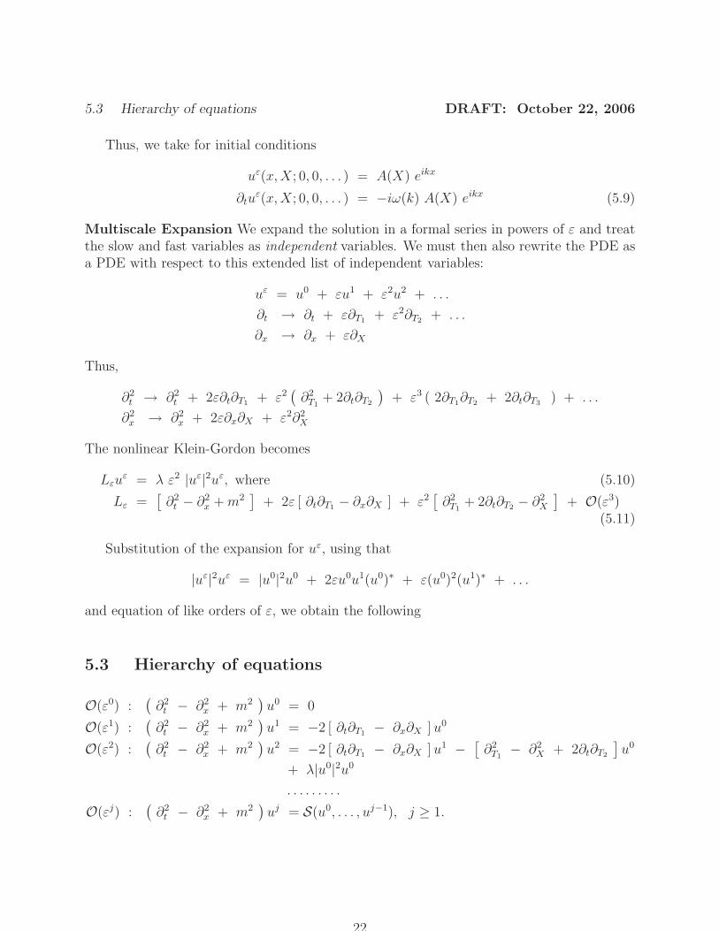
Thus, we take for initial conditions

uε(x,X; 0, 0, . . . ) = A(X) eikx

∂tuε(x,X; 0, 0, . . . ) = −iω(k) A(X) eikx (5.9)

Multiscale Expansion We expand the solution in a formal series in powers of ε and treatthe slow and fast variables as independent variables. We must then also rewrite the PDE asa PDE with respect to this extended list of independent variables:

uε = u0 + εu1 + ε2u2 + . . .

∂t → ∂t + ε∂T1 + ε2∂T2 + . . .

∂x → ∂x + ε∂X

Thus,

∂2t → ∂2

t + 2ε∂t∂T1 + ε2(∂2

T1+ 2∂t∂T2

)+ ε3 ( 2∂T1∂T2 + 2∂t∂T3 ) + . . .

∂2x → ∂2

x + 2ε∂x∂X + ε2∂2X

The nonlinear Klein-Gordon becomes

Lεuε = λ ε2 |uε|2uε, where (5.10)

Lε =[∂2

t − ∂2x +m2

]+ 2ε [ ∂t∂T1 − ∂x∂X ] + ε2

[∂2

T1+ 2∂t∂T2 − ∂2

X

]+ O(ε3)

(5.11)

Substitution of the expansion for uε, using that

|uε|2uε = |u0|2u0 + 2εu0u1(u0)∗ + ε(u0)2(u1)∗ + . . .

and equation of like orders of ε, we obtain the following

5.3 Hierarchy of equations

O(ε0) :(∂2

t − ∂2x + m2

)u0 = 0

O(ε1) :(∂2

t − ∂2x + m2

)u1 = −2 [ ∂t∂T1 − ∂x∂X ] u0

O(ε2) :(∂2

t − ∂2x + m2

)u2 = −2 [ ∂t∂T1 − ∂x∂X ] u1 −

[∂2

T1− ∂2

X + 2∂t∂T2

]u0

+ λ|u0|2u0

. . . . . . . . .

O(εj) :(∂2

t − ∂2x + m2

)uj = S(u0, . . . , uj−1), j ≥ 1.

22

5.4 Solution of equation hierarchy DRAFT: October 22, 2006

5.4 Solution of equation hierarchy

O(ε0): We take u0 to be a plane wave solution:

u0(x,X; t, T1, T2, . . . ) = A(X;T1, T2, . . . ) ei(kx−ω(k)t) (5.12)

The slowly varying amplitude, A, is to be determined at higher order in the perturbationscheme.

O(ε1): Using the expression (5.12) for u0, we find that u1 satisfies:

(∂2

t − ∂2x + m2

)u0 = −2 [ ∂t∂T1 − ∂x∂X ] u0

= 2i [ ω(k)∂T1A + k ∂XA ] ei(kx−ω(k)t)

= 2iω(k)

[∂T1A +

k

ω(k)∂XA

]ei(kx−ω(k)t)

= 2iω(k) [ ∂T1A + ω′(k)∂XA ] ei(kx−ω(k)t), (5.13)

where we have used that ω2 = m2 + k2 and therefore ω′(k) = k/ω(k).

Exercise 5.1 Prove the following

Proposition 5.1 If α 6= 0, then the PDE

(∂2

t − ∂2x + m2

)U = α ei(kx−ω(k)t

has resonant forcing and its general solution grows linearly in time.

It follows that the expansion uε = u0 + εu1 + . . . will break down on times of order ε−1

in the sense that εu1 will become comparable in size with u0 unless A is constrained so thatthe right hand side of (5.13) vanishes. This gives the equation:

∂T1 A + ω′(k) ∂X A = 0 (5.14)

Equation (5.14) implies that the amplitude propagates with the group velocity, ω′(k). Wehave

A = A(Y, T2, . . . ), where Y = X − ω′(k)T1

Furthermore, u1 is now seen to satisfy a homogeneous equation and we take u1 ≡ 0. Thesolution we have thus far constructed is

uε = A(X − ω′(k)T1, T2, . . . ) ei(kx−ω(k)t) + ε2u2 + . . .

Using that u1 = 0 as well as the expression for u0 we obtain the following equation for u2:

(∂2

t − ∂2x + m2

)u2 =

[2iω(k)∂T2A −

(∂2

T1− ∂2

X

)A + λ|A|2A

]ei(kx−ω(k)t) (5.15)

By Proposition 5.1 we require

2iω(k)∂T2A −(∂2

T1− ∂2

X

)A + λ|A|2A = 0 (5.16)

23

5.5 Conclusion and Theorem DRAFT: October 22, 2006

We can simplify (5.16) by making the following observations:

∂T1 = −ω′∂Y , ∂Y = ∂X , ∂2T1

− ∂2X =

((ω′)2 − 1

)∂2

Y

This gives2iω(k)∂T2A +

(1 − (ω′)2

)∂2

YA + λ|A|2A = 0 (5.17)

Finally, note that

ω2 = m2 + k2 =⇒ ωω′ = k =⇒ ωω′′ + (ω′)2 = 1

Thus,2iω(k)∂T2A + ω(k)ω′′(k) ∂2

YA + λ|A|2A = 0 (5.18)

5.5 Conclusion and Theorem

Definition We call a wave equation strongly dispersive at wave number k0 if its dispersionrelation satisfies ω′′(k0) 6= 0.

Conclusion: A nearly monochromatic (about wave number k) wave packet in a stronglydispersive system will translate with the group velocity, ω′(k), and modulate in accordancewith the nonlinear Schrodinger equation (5.18).

The following result can be proved:

Theorem 5.1 Let A(Y, T2) satisfy the nonlinear Schrodinger equation (5.18). There existsa small constant ε0 > 0, such that for any τ > 0 and ε < ε0, the nonlinear Klein-Gordonequation (5.4) has solutions

v(x, t) = ε[A(ε(x− ω′(k)t), ε2t) ei(kx−ω(k)t) + ε wε(x, t)

],

where wε satisfies the following bound:

‖ wε(·, t) ‖H1(IR)

≤ C1, |wε(x, t)| ≤ C2, 0 ≤ t ≤ τε−2

6 Structural Properties of NLS

6.1 Hamiltonian structure

6.2 Symmetries and conserved integrals

7 Formulation in H1 and the basic well-posedness the-

orem

8 Special solutions of NLS - nonlinear plane waves and

nonlinear bound states

24


9 Appendices

9.1 The M. Riesz Convexity Theorem

A linear operator, T , is of type (p, q), where p−1 + q−1 = 1, if there exists a positive constantk such that for all f ∈ Lp

‖Tf‖q ≤ k ‖f‖p (9.1)

Theorem 9.1 [5] Let T be of type (pi, qi) with norm ki, i = 0, 1. Then, T is of type (pθ, qθ)with (pθ, qθ) norm

kθ ≤ k1−θ0 kθ

1, (9.2)

provided(p−1

θ , q−1θ ) = (1 − θ)(p−1

0 , q−10 ) + θ(p−1

1 , q−11 ) (9.3)

9.2 The Implicit Function Theorem

Definition 9.1 A mapping between Banach spaces X and Z, F : X → Z, is (Frechet)differentiable if there is a bounded linear transformation L : X → Z, such that

‖F (x+ ξ) − F (x) − Lξ‖Z = o(‖ξ‖X)

as |ξ‖X → 0.

Theorem 9.2 [2] Let X, Y and Z denote Banach spaces. Let F denote a continuous map-ping

F : U ⊂ X × Y → Z, (x, y) 7→ F (x, y),

where U is open. Assume F is (Frechet) differentiable with respect to x and that Fx(x, y)is continuous in U . Let (x0, y0) ∈ U and F (x0, y0) = 0. If the linear operator η 7→ Lη ≡Fx(x0, y0)η is one to one and onto Z (an isomorphism from X to Z), then

(i) There exists a ball y : ‖y − y0‖Y < r = Br(y0) and a unique continuous mappingu : Br(y0) → X such that u(y0) = x0 and F (u(y), y) = 0.

(ii) uy ∈ Cp if F ∈ Cp, 1 < p ≤ ∞.

Remark 9.1 IfX = IRm, Y = IRn and Z = IRm, this reduces to the usual finite dimensionalcase. The m by m matrix, Fx(x0, y0), is assumed to be invertible.

9.3 The Contraction Mapping Principle

Theorem 9.3 Let T : X → X denote a mapping from a complete metric space, X, intoitself. Assume that T is a contraction on X, i.e. there exists k with 0 < k < 1, such thatfor any α and β in X

ρ(Tα, Tβ) ≤ k ρ(α, β) (9.4)

Then, there exists a unique element of X, α∗, for which Tα∗ = α∗. Moreover, starting with anarbitrary element α0 ∈ X and defining αj = Tαj−1, j = 1, 2, 3, . . . , we have α∗ = limj→∞ αj.

25

REFERENCES DRAFT: October 22, 2006

References

[1] G. Folland. Introduction to Partial Differential Equations. Princeton, (1976).

[2] L. Nirenberg. Lectures on Nonlinear Functional Analysis. Courant Institute, New York,1974.

[3] M. Reed and B. Simon. Modern Methods of Mathematical Physics - Volume 1 - FunctionalAnalysis. Academic Press.

[4] E.M. Stein. Harmonic Analysis - Real Variable Methods, Orthogonality and OscillatoryIntegrals. Princeton, 1993.

[5] E.M. Stein and G. Weiss. Introduction to Fourier Analysis on Euclidean Spaces. Prince-ton, 1971.

[6] G.B. Whitham. Linear and Nonlinear Waves. Wiley, 1974.

26

lectures on linear and nonlinear dispersive waves draft...

Documents