lectures on machine learning - lecture 3: practical aspects of machine...
TRANSCRIPT

Lectures on Machine Learning
Lecture 3: practical aspects of machine learning
Stefano Carrazza
TAE2018, 2-15 September 2018
European Organization for Nuclear Research (CERN)
Acknowledgement: This project has received funding from HICCUP ERC Consolidatorgrant (614577) and by the European Unions Horizon 2020 research and innovationprogramme under grant agreement no. 740006.
PDFN 3Machine Learning • PDFs • QCD

Outline
Lecture 1 (yesterday)
• Artificial intelligence
• Machine learning
• Model representation
• Metrics
Lecture 2 (today)
• Parameter learning
• Non-linear models
• Beyond neural networks
• Clustering
Lecture 3 (today)
• Hyperparameter tune
• Cross-validation
• ML in practice
• The PDF case study
1
Hyperparameter tune
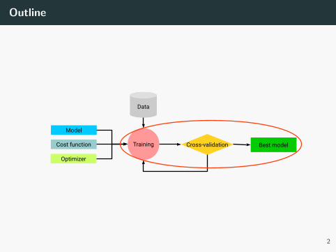
Outline
Model
Optimizer
Cost function Best modelCross-validationTraining
Data
2
Hyperparameters summary
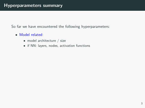
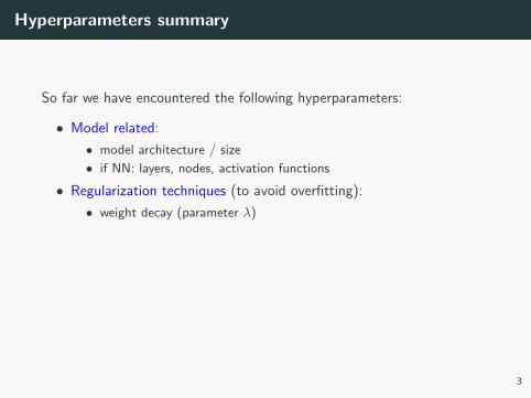
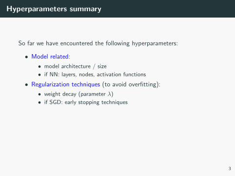
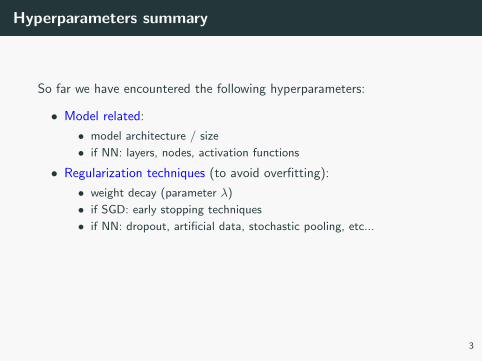
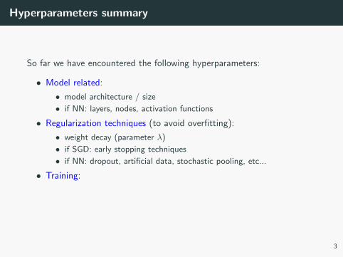
So far we have encountered the following hyperparameters:
• Model related:
• model architecture / size
• if NN: layers, nodes, activation functions
• Regularization techniques (to avoid overfitting):
• weight decay (parameter λ)
• if SGD: early stopping techniques
• if NN: dropout, artificial data, stochastic pooling, etc...
• Training:
• the SGD learning parameters η
• other SGD parameters depending on the gradient descent scheme
3
Hyperparameters summary
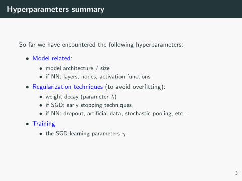
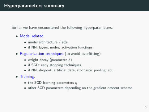
So far we have encountered the following hyperparameters:
• Model related:
• model architecture / size
• if NN: layers, nodes, activation functions
• Regularization techniques (to avoid overfitting):
• weight decay (parameter λ)
• if SGD: early stopping techniques
• if NN: dropout, artificial data, stochastic pooling, etc...
• Training:
• the SGD learning parameters η
• other SGD parameters depending on the gradient descent scheme
3

Hyperparameters summary
So far we have encountered the following hyperparameters:
• Model related:
• model architecture / size
• if NN: layers, nodes, activation functions
• Regularization techniques (to avoid overfitting):
• weight decay (parameter λ)
• if SGD: early stopping techniques
• if NN: dropout, artificial data, stochastic pooling, etc...
• Training:
• the SGD learning parameters η
• other SGD parameters depending on the gradient descent scheme
3
Other regularization techniques
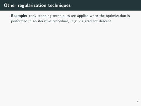
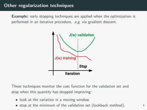
Example: early stopping techniques are applied when the optimization is
performed in an iterative procedure, .e.g. via gradient descent.
Iteration
J(w) training
J(w) validation
Stop
These techniques monitor the cost function for the validation set and
stop when this quantity has stopped improving:
• look at the variation in a moving window
• stop at the minimum of the validation set (lookback method),
4
Other regularization techniques
Example: early stopping techniques are applied when the optimization is
performed in an iterative procedure, .e.g. via gradient descent.
Iteration
J(w) training
J(w) validation
Stop
These techniques monitor the cost function for the validation set and
stop when this quantity has stopped improving:
• look at the variation in a moving window
• stop at the minimum of the validation set (lookback method), 4
Other regularization techniques
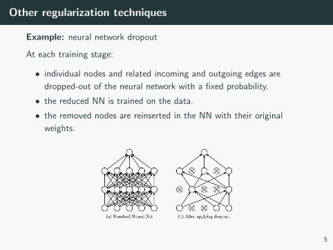
Example: neural network dropout
At each training stage:
• individual nodes and related incoming and outgoing edges are
dropped-out of the neural network with a fixed probability.
• the reduced NN is trained on the data.
• the removed nodes are reinserted in the NN with their original
weights.
5

Other regularization techniques
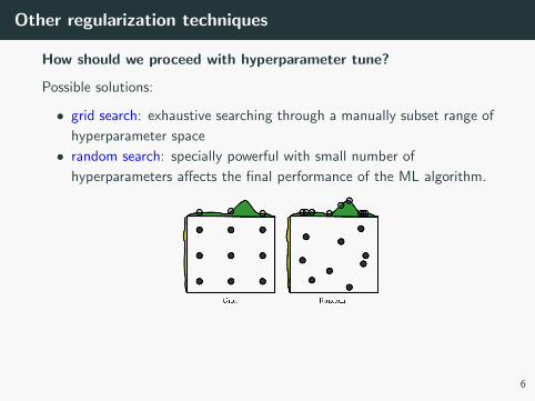
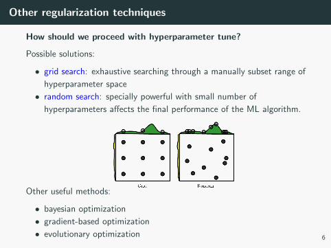
How should we proceed with hyperparameter tune?
Possible solutions:
• grid search: exhaustive searching through a manually subset range of
hyperparameter space
• random search: specially powerful with small number of
hyperparameters affects the final performance of the ML algorithm.
Other useful methods:
• bayesian optimization
• gradient-based optimization
• evolutionary optimization
6
Other regularization techniques
How should we proceed with hyperparameter tune?
Possible solutions:
• grid search: exhaustive searching through a manually subset range of
hyperparameter space
• random search: specially powerful with small number of
hyperparameters affects the final performance of the ML algorithm.
Other useful methods:
• bayesian optimization
• gradient-based optimization
• evolutionary optimization 6

Cross-validation
Cross-validation
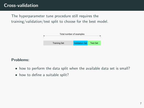
The hyperparameter tune procedure still requires the
training/validation/test split to choose for the best model.
Training Set Test Set
Total number of examples
Validation Set
Problems:
• how to perform the data split when the available data set is small?
• how to define a suitable split?
Solution:
Use cross-validation algorithms to access the quality of your model +
hyperparameter choice.
7

Cross-validation
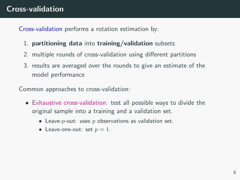
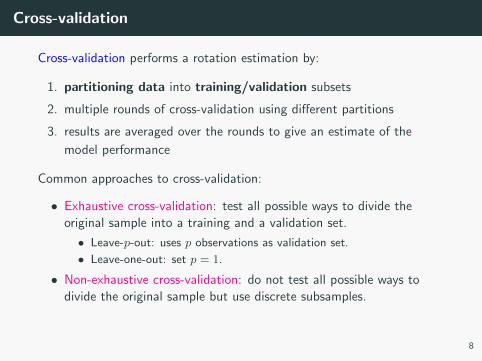
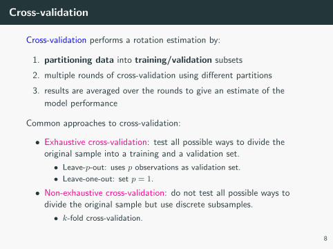
Cross-validation performs a rotation estimation by:
1. partitioning data into training/validation subsets
2. multiple rounds of cross-validation using different partitions
3. results are averaged over the rounds to give an estimate of the
model performance
Common approaches to cross-validation:
• Exhaustive cross-validation: test all possible ways to divide the
original sample into a training and a validation set.
• Leave-p-out: uses p observations as validation set.
• Leave-one-out: set p = 1.
• Non-exhaustive cross-validation: do not test all possible ways to
divide the original sample but use discrete subsamples.
• k-fold cross-validation.
8
Cross-validation
Cross-validation performs a rotation estimation by:
1. partitioning data into training/validation subsets
2. multiple rounds of cross-validation using different partitions
3. results are averaged over the rounds to give an estimate of the
model performance
Common approaches to cross-validation:
• Exhaustive cross-validation: test all possible ways to divide the
original sample into a training and a validation set.
• Leave-p-out: uses p observations as validation set.
• Leave-one-out: set p = 1.
• Non-exhaustive cross-validation: do not test all possible ways to
divide the original sample but use discrete subsamples.
• k-fold cross-validation.
8
Example k-fold cross-validation
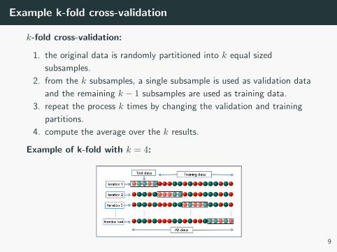
k-fold cross-validation:
1. the original data is randomly partitioned into k equal sized
subsamples.
2. from the k subsamples, a single subsample is used as validation data
and the remaining k − 1 subsamples are used as training data.
3. repeat the process k times by changing the validation and training
partitions.
4. compute the average over the k results.
Example of k-fold with k = 4:
9
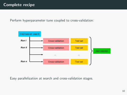
Complete recipe
Perform hyperparameter tune coupled to cross-validation:
Best solution
Grid/random search
Cross-validation Test set
Cross-validation Test set
Cross-validation Test set
... ...
Run I
Run II
Run n
Easy parallelization at search and cross-validation stages.
10

Closure testing
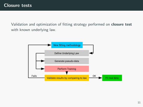
Closure tests
Validation and optimization of fitting strategy performed on closure test
with known underlying law.
New fitting methodology
Define Underlying Law
Generate pseudo-data
Validate results by comparing to law
Perform Training
Fit real dataFails OK
11
ML in practice
Most popular public ML frameworks
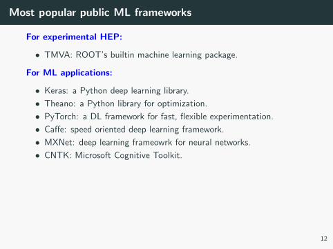
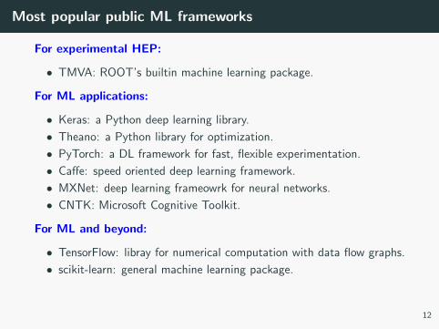
For experimental HEP:
• TMVA: ROOT’s builtin machine learning package.
For ML applications:
• Keras: a Python deep learning library.
• Theano: a Python library for optimization.
• PyTorch: a DL framework for fast, flexible experimentation.
• Caffe: speed oriented deep learning framework.
• MXNet: deep learning frameowrk for neural networks.
• CNTK: Microsoft Cognitive Toolkit.
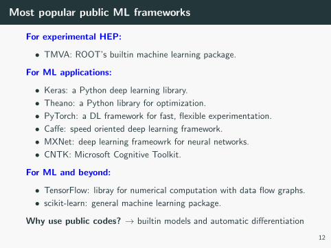
For ML and beyond:
• TensorFlow: libray for numerical computation with data flow graphs.
• scikit-learn: general machine learning package.
Why use public codes? → builtin models and automatic differentiation
12
Most popular public ML frameworks
For experimental HEP:
• TMVA: ROOT’s builtin machine learning package.
For ML applications:
• Keras: a Python deep learning library.
• Theano: a Python library for optimization.
• PyTorch: a DL framework for fast, flexible experimentation.
• Caffe: speed oriented deep learning framework.
• MXNet: deep learning frameowrk for neural networks.
• CNTK: Microsoft Cognitive Toolkit.
For ML and beyond:
• TensorFlow: libray for numerical computation with data flow graphs.
• scikit-learn: general machine learning package.
Why use public codes? → builtin models and automatic differentiation
12
Keras
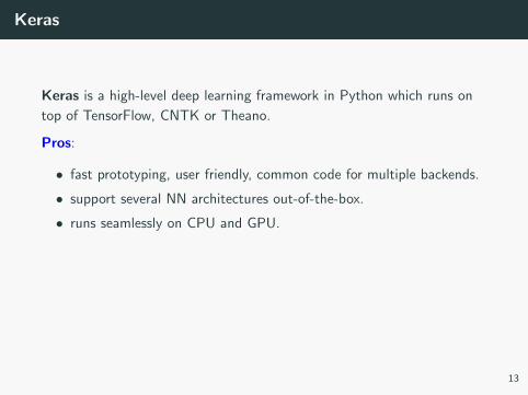
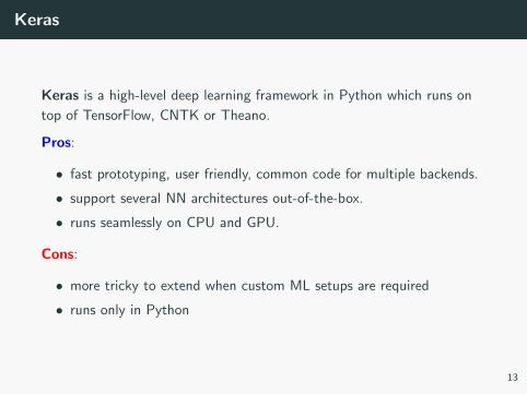
Keras is a high-level deep learning framework in Python which runs on
top of TensorFlow, CNTK or Theano.
Pros:
• fast prototyping, user friendly, common code for multiple backends.
• support several NN architectures out-of-the-box.
• runs seamlessly on CPU and GPU.
Cons:
• more tricky to extend when custom ML setups are required
• runs only in Python
13
Keras
Keras is a high-level deep learning framework in Python which runs on
top of TensorFlow, CNTK or Theano.
Pros:
• fast prototyping, user friendly, common code for multiple backends.
• support several NN architectures out-of-the-box.
• runs seamlessly on CPU and GPU.
Cons:
• more tricky to extend when custom ML setups are required
• runs only in Python
13
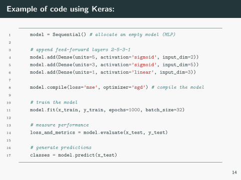
Example of code using Keras:
1 model = Sequential() # allocate an empty model (MLP)
2
3 # append feed-forward layers 2-5-3-1
4 model.add(Dense(units=5, activation=’sigmoid’, input_dim=2))
5 model.add(Dense(units=3, activation=’sigmoid’, input_dim=5))
6 model.add(Dense(units=1, activation=’linear’, input_dim=3))
7
8 model.compile(loss=’mse’, optimizer=’sgd’) # compile the model
9
10 # train the model
11 model.fit(x_train, y_train, epochs=1000, batch_size=32)
12
13 # measure performance
14 loss_and_metrics = model.evaluate(x_test, y_test)
15
16 # generate predictions
17 classes = model.predict(x_test)
14
TensorFlow
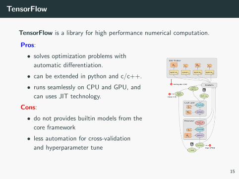
TensorFlow is a library for high performance numerical computation.
Pros:
• solves optimization problems with
automatic differentiation.
• can be extended in python and c/c++.
• runs seamlessly on CPU and GPU, and
can uses JIT technology.
Cons:
• do not provides builtin models from the
core framework
• less automation for cross-validation
and hyperparameter tune
15
TensorFlow
TensorFlow is a library for high performance numerical computation.
Pros:
• solves optimization problems with
automatic differentiation.
• can be extended in python and c/c++.
• runs seamlessly on CPU and GPU, and
can uses JIT technology.
Cons:
• do not provides builtin models from the
core framework
• less automation for cross-validation
and hyperparameter tune
15
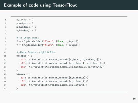
Example of code using TensorFlow:
1 n_intput = 2
2 n_output = 1
3 n_hidden_1 = 5
4 n_hidden_2 = 3
5
6 # tf Graph input
7 X = tf.placeholder("float", [None, n_input])
8 Y = tf.placeholder("float", [None, n_output])
9
10 # Store layers weight & bias
11 weights = {
12 ’h1’: tf.Variable(tf.random_normal([n_input, n_hidden_1])),
13 ’h2’: tf.Variable(tf.random_normal([n_hidden_1, n_hidden_2])),
14 ’out’: tf.Variable(tf.random_normal([n_hidden_2, n_output]))
15 }
16 biases = {
17 ’b1’: tf.Variable(tf.random_normal([n_hidden_1])),
18 ’b2’: tf.Variable(tf.random_normal([n_hidden_2])),
19 ’out’: tf.Variable(tf.random_normal([n_output]))
20 }
16
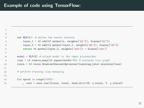
Example of code using TensorFlow:
1 ...
2
3 def MLP(x): # define the neural network
4 layer_1 = tf.add(tf.matmul(x, weights[’h1’]), biases[’b1’])
5 layer_2 = tf.add(tf.matmul(layer_1, weights[’h2’]), biases[’b2’])
6 return tf.matmul(layer_2, weights[’out’]) + biases[’out’]
7
8 model = MLP(X) # attach model to the input placeholder
9 loss = tf.reduce_mean(tf.square(model-Y)) # evaluate loss graph
10 train = tf.train.GradientDescentOptimizer(learning_rate).minimize(loss)
11
12 # perform training loop manually
13 ...
14 for epoch in range(1000):
15 _, cost = sess.run([train, loss], feed_dict={X: x_train, Y: y_train})
17

Scikit-learn
18
Scikit-learn
Scikit-learn contains the most popular algorithms for:
• Supervised learning: neural networks, decision trees, etc.
• Unsupervised learning: density estimate, clustering, etc.
• Model selection: cross-validation, hyperparameter tune, etc.
• Dataset transformations: feature extractions, dim. reduction, etc.
• Dataset loading
• Strategies to scale computationally
• Computational performance
19

The PDF case study
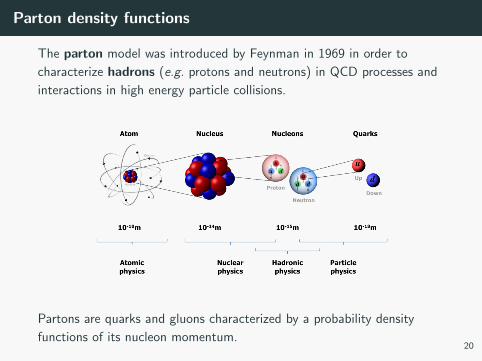
Parton density functions
The parton model was introduced by Feynman in 1969 in order to
characterize hadrons (e.g. protons and neutrons) in QCD processes and
interactions in high energy particle collisions.
Partons are quarks and gluons characterized by a probability density
functions of its nucleon momentum.20
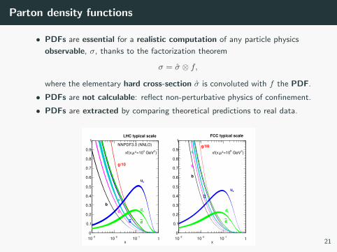
Parton density functions
• PDFs are essential for a realistic computation of any particle physics
observable, σ, thanks to the factorization theorem
σ = σ ⊗ f,
where the elementary hard cross-section σ is convoluted with f the PDF.
• PDFs are not calculable: reflect non-perturbative physics of confinement.
• PDFs are extracted by comparing theoretical predictions to real data.
x
3−
102−
101−
10 1
0
0.1
0.2
0.3
0.4
0.5
0.6
0.7
0.8
0.9
1
g/10
vu
vd
d
c
s
u
b
NNPDF3.0 (NNLO)
)2
GeV4
=102µxf(x,
LHC typical scale
x
3−
102−
101−
10 1
0
0.1
0.2
0.3
0.4
0.5
0.6
0.7
0.8
0.9
1
g/10
vu
vd
d
u
s
c
b
)2
GeV8
=102µxf(x,
FCC typical scale
21
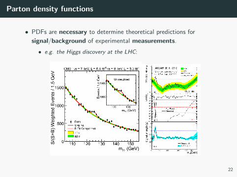
Parton density functions
• PDFs are necessary to determine theoretical predictions for
signal/background of experimental measurements.
• e.g. the Higgs discovery at the LHC:
22
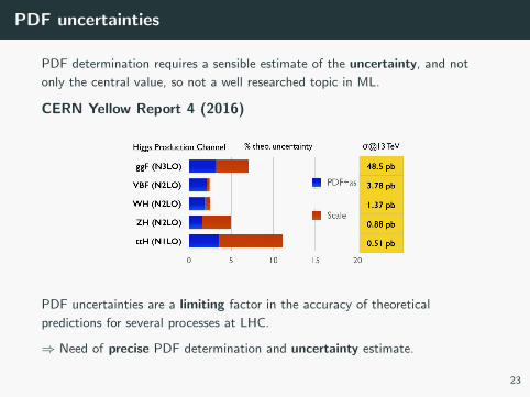
PDF uncertainties
PDF determination requires a sensible estimate of the uncertainty, and not
only the central value, so not a well researched topic in ML.
CERN Yellow Report 4 (2016)
PDF uncertainties are a limiting factor in the accuracy of theoretical
predictions for several processes at LHC.
⇒ Need of precise PDF determination and uncertainty estimate.
23
Why ML in PDFs determination?
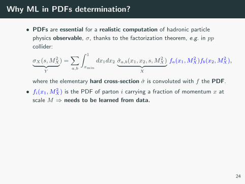
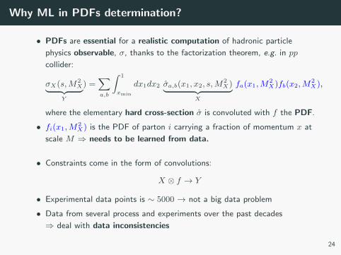
• PDFs are essential for a realistic computation of hadronic particle
physics observable, σ, thanks to the factorization theorem, e.g. in pp
collider:
σX(s,M2X︸ ︷︷ ︸
Y
) =∑a,b
∫ 1
xmin
dx1dx2 σa,b(x1, x2, s,M2X)︸ ︷︷ ︸
X
fa(x1,M2X)fb(x2,M
2X),
where the elementary hard cross-section σ is convoluted with f the PDF.
• fi(x1,M2X) is the PDF of parton i carrying a fraction of momentum x at
scale M ⇒ needs to be learned from data.
• Constraints come in the form of convolutions:
X ⊗ f → Y
• Experimental data points is ∼ 5000 → not a big data problem
• Data from several process and experiments over the past decades
⇒ deal with data inconsistencies
24
Why ML in PDFs determination?
• PDFs are essential for a realistic computation of hadronic particle
physics observable, σ, thanks to the factorization theorem, e.g. in pp
collider:
σX(s,M2X︸ ︷︷ ︸
Y
) =∑a,b
∫ 1
xmin
dx1dx2 σa,b(x1, x2, s,M2X)︸ ︷︷ ︸
X
fa(x1,M2X)fb(x2,M
2X),
where the elementary hard cross-section σ is convoluted with f the PDF.
• fi(x1,M2X) is the PDF of parton i carrying a fraction of momentum x at
scale M ⇒ needs to be learned from data.
• Constraints come in the form of convolutions:
X ⊗ f → Y
• Experimental data points is ∼ 5000 → not a big data problem
• Data from several process and experiments over the past decades
⇒ deal with data inconsistencies
24

ML and PDF determination
The NNPDF methodology
The NNPDF (Neural Networks PDF) implements the Monte Carlo
approach to the determination of a global PDF fit. We propose to:
1. reduce all sources of theoretical bias:
• no fixed functional form
• possibility to reproduce non-Gaussian behavior
⇒ use Neural Networks instead of polynomials
2. provide a sensible estimate of the uncertainty:
• uncertainties from input experimental data
• minimization inefficiencies and degenerate minima
• theoretical uncertainties
⇒ use MC artificial replicas from data, training with a GA minimizer
3. Test the setup through closure tests
25
Experimental data
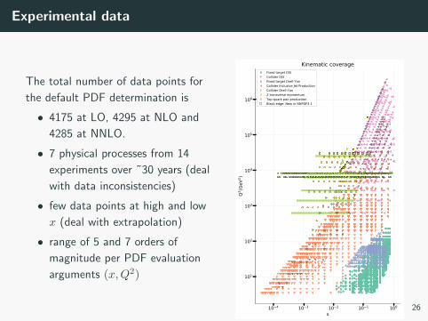
The total number of data points for
the default PDF determination is
• 4175 at LO, 4295 at NLO and
4285 at NNLO.
• 7 physical processes from 14
experiments over ˜30 years (deal
with data inconsistencies)
• few data points at high and low
x (deal with extrapolation)
• range of 5 and 7 orders of
magnitude per PDF evaluation
arguments (x,Q2)
10 4 10 3 10 2 10 1 100
x
101
102
103
104
105
106
Q2 (Ge
V2 )
Kinematic coverageFixed target DISCollider DISFixed target Drell-YanCollider Inclusive Jet ProductionCollider Drell-YanZ transverse momentumTop-quark pair productionBlack edge: New in NNPDF3.1
26
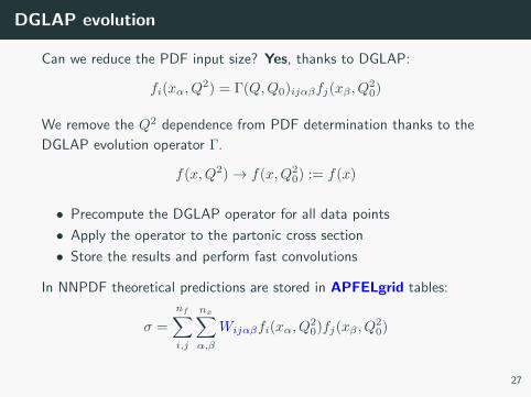
DGLAP evolution
Can we reduce the PDF input size? Yes, thanks to DGLAP:
fi(xα, Q2) = Γ(Q,Q0)ijαβfj(xβ , Q
20)
We remove the Q2 dependence from PDF determination thanks to the
DGLAP evolution operator Γ.
f(x,Q2)→ f(x,Q20) := f(x)
• Precompute the DGLAP operator for all data points
• Apply the operator to the partonic cross section
• Store the results and perform fast convolutions
In NNPDF theoretical predictions are stored in APFELgrid tables:
σ =
nf∑i,j
nx∑α,β
Wijαβfi(xα, Q20)fj(xβ , Q
20)
27
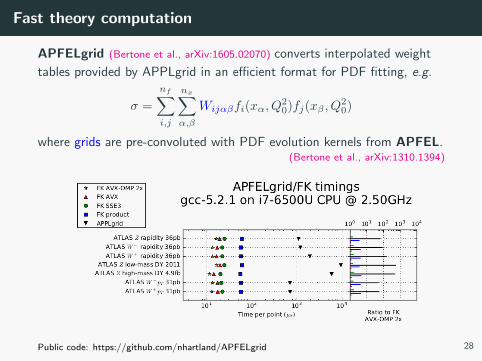
Fast theory computation
APFELgrid (Bertone et al., arXiv:1605.02070) converts interpolated weight
tables provided by APPLgrid in an efficient format for PDF fitting, e.g.
σ =
nf∑i,j
nx∑α,β
Wijαβfi(xα, Q20)fj(xβ , Q
20)
where grids are pre-convoluted with PDF evolution kernels from APFEL.(Bertone et al., arXiv:1310.1394)
Public code: https://github.com/nhartland/APFELgrid 28
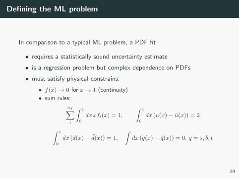
Defining the ML problem
In comparison to a typical ML problem, a PDF fit
• requires a statistically sound uncertainty estimate
• is a regression problem but complex dependence on PDFs
• must satisfy physical constrains:
• f(x)→ 0 for x→ 1 (continuity)
• sum rules:
nf∑i
∫ 1
0
dxxfi(x) = 1,
∫ 1
0
dx (u(x)− u(x)) = 2
∫ 1
0
dx (d(x)− d(x)) = 1,
∫dx (q(x)− q(x)) = 0, q = s, b, t
29
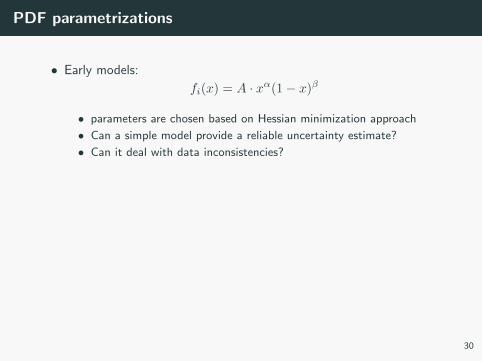
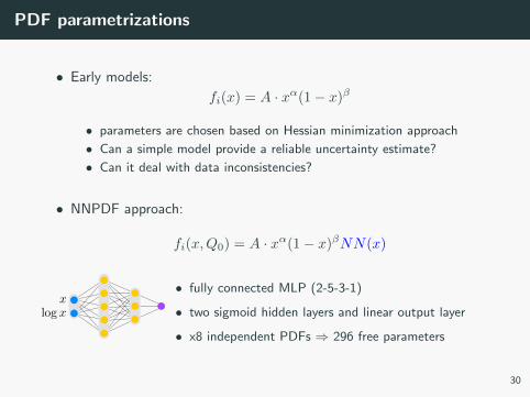
PDF parametrizations
• Early models:
fi(x) = A · xα(1− x)β
• parameters are chosen based on Hessian minimization approach
• Can a simple model provide a reliable uncertainty estimate?
• Can it deal with data inconsistencies?
• NNPDF approach:
fi(x,Q0) = A · xα(1− x)βNN(x)
• fully connected MLP (2-5-3-1)
• two sigmoid hidden layers and linear output layer
• x8 independent PDFs ⇒ 296 free parameters
30
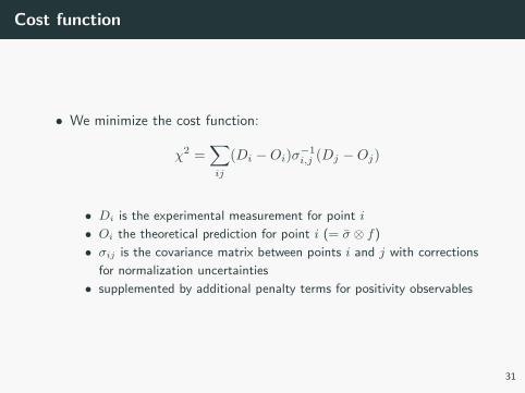
Cost function
• We minimize the cost function:
χ2 =∑ij
(Di −Oi)σ−1i,j (Dj −Oj)
• Di is the experimental measurement for point i
• Oi the theoretical prediction for point i (= σ ⊗ f)
• σij is the covariance matrix between points i and j with corrections
for normalization uncertainties
• supplemented by additional penalty terms for positivity observables
31
Propagating experimental uncertainties
Generate artificial Monte Carlo data replicas from experimental data.
We perform Nrep O(1000) fits, sampling pseudodata replicas:
D(r)i → D
(r)i + chol(Σ)i,jN (0, 1), i, j = 1..Ndat, r = 1...Nrep
We obtain Nrep PDF replicas. No assumptions at all about the
Gaussianity of the errors.
We perform compression techniques for PDF delivery:
• CMC-PDFs: compression algorithm for MC PDFs.
• mc2hessian: MC to hessian conversion tool for PDFs.
• SMPDF: Specialized Minimal PDFs.
PDF releases reduce 1000 replicas to 100.
32
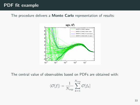
PDF fit example
The procedure delivers a Monte Carlo representation of results:
510 410
310 210 110
2
1
0
1
2
3
4
5
6
7
)2xg(x, Q
NNPDF 2.3 NNLO replicas
NNPDF 2.3 NNLO mean value
error bandσNNPDF 2.3 NNLO 1
NNPDF 2.3 NNLO 68% CL band
)2xg(x, Q
The central value of observables based on PDFs are obtained with:
〈O[f ]〉 =1
Nrep
Nrep∑k=1
O[fk]
33
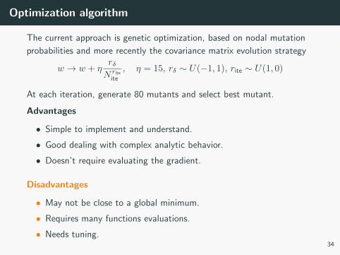
Optimization algorithm
The current approach is genetic optimization, based on nodal mutation
probabilities and more recently the covariance matrix evolution strategy
w → w + ηrδNrite
ite
, η = 15, rδ ∼ U(−1, 1), rite ∼ U(1, 0)
At each iteration, generate 80 mutants and select best mutant.
Advantages
• Simple to implement and understand.
• Good dealing with complex analytic behavior.
• Doesn’t require evaluating the gradient.
Disadvantages
• May not be close to a global minimum.
• Requires many functions evaluations.
• Needs tuning.34
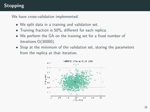
Stopping
We have cross-validation implemented:
• We split data in a training and validation set.
• Training fraction is 50%, different for each replica.
• We perform the GA on the training set for a fixed number of
iterations O(30000).
• Stop at the minimum of the validation set, storing the parameters
from the replica at that iteration.
35
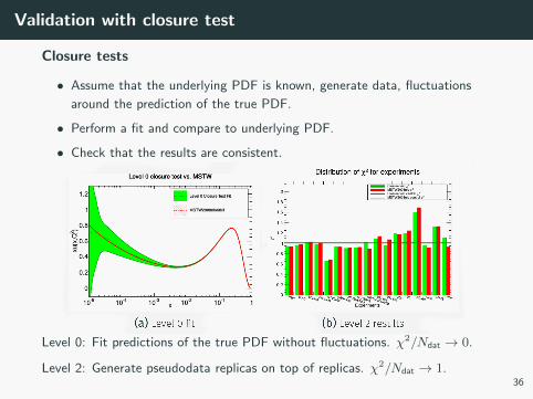
Validation with closure test
Closure tests
• Assume that the underlying PDF is known, generate data, fluctuations
around the prediction of the true PDF.
• Perform a fit and compare to underlying PDF.
• Check that the results are consistent.
Level 0: Fit predictions of the true PDF without fluctuations. χ2/Ndat → 0.
Level 2: Generate pseudodata replicas on top of replicas. χ2/Ndat → 1.36

Summary

Summary
We have covered the following topics:
• The hyperparameter tune
• the cross-validation techniques
• ML frameworks
• The PDF case study
37