legan: disentangled manipulation of directional lighting

LEGAN: Disentangled Manipulation of Directional Lighting and FacialExpressions whilst Leveraging Human Perceptual Judgements (Supplementary

Text)

Sandipan Banerjee1, Ajjen Joshi1, Prashant Mahajan*2, Sneha Bhattacharya*3, Survi Kyal1

and Taniya Mishra*4

1Affectiva, USA, 2Amazon, USA, 3Silver Spoon Animation, USA, 4SureStart, USA{firstname.lastname}@affectiva.com, [email protected], [email protected],

[email protected]

1. Quality Estimation Model: Architecture De-tails

We share details of the architecture of our quality esti-mator Q in Table 1. The fully connected layers in Q aredenoted as ‘fc’ while each convolution layer, represented as‘conv’, is followed by Leaky ReLU [20] activation with aslope of 0.01.

Table 1: Detailed architecture of our quality estimation model Q (inputsize is 128×128×3).

Layer Filter/Stride/Dilation # of filtersinput 128×128 3conv0 4×4/2/1 64conv1 4×4/2/1 128conv2 4×4/2/1 256conv3 4×4/2/1 512conv4 4×4/2/1 1024conv5 4×4/2/1 2048

fc0 - 256fc1 - 1

2. Quality Estimation Model: Naturalness Rat-ing Distribution in Training

In this section, we share the distribution of the natural-ness ratings that we collected from the Amazon MechanicalTurk (AMT) experiment (Stage II). To do this, we averagethe perceptual rating for each synthetic face image from itsthree scores and increment the count of a particular bin in[(0 - 1), (1 - 2), ... , (8 - 9), (9 - 10)] based on the mean score.As described in Section 3 of the main paper, we design theAMT task such that a mean rating between 0 and 5 sug-gests the synthetic image to look ‘unnatural’ while a scorebetween 5 and 10 advocates for its naturalness. As can be

*Work done while at Affectiva

Table 2: Hourglass architecture for expression mask (Me) synthesis in thegenerator G. The input size is 128×128×9, three RGB channels (Ia) andsix expression channels (ce).

Layer Filter/Stride/Dilation # of filtersinput 128×128/-/- 9conv0 7×7/1/1 64conv1 4×4/2/1 128conv2 4×4/2/1 256RB0 3×3/1/1 256RB1 3×3/1/1 256RB2 3×3/1/1 256RB3 3×3/1/1 256RB4 3×3/1/1 256RB5 3×3/1/1 256PS0 - 256

conv3 4×4/1/1 128PS1 - 128

conv4 4×4/1/1 64conv5 (Me) 7×7/1/1 3

seen in Figure 1, majority of the synthetic images used inour study generates a mean score that falls on the ‘natural’side, validating their realism. When used to train our qual-ity estimation model Q, these images tune its weights tolook for the same perceptual features in other images whilerating their naturalness.

To further check the overall perceptual quality of eachof the different synthesis approaches used in our study [10,11, 1, 15, 3], we separately find the mean rating for eachsynthetic face image generated by that method, depicted inFigure 2. It comes as no surprise for the StyleGAN [11]images to rank the highest, with a mean score over 7, as itsface images were pre-filtered for quality [2]. The other fourapproaches perform roughly the same, generating a meanscore that falls between 6 and 7.

Figure 1: Histogram depicting the number of images in each naturalness bin, as rated by the Amazon Mechanical Turkers. Much more images fell on the‘natural’ half (5 - 10) rather than the ‘unnatural’ one (0 - 5), suggesting the synthetic face images used in our study to be more or less realistic.

Figure 2: Mean naturalness rating of the different synthesis approaches used in our study [10, 11, 1, 15, 3]. As expected, the StyleGAN [11] images arerated higher than others as they were pre-filtered for quality[2].

3. Quality Estimation Model: Loss Function

Our loss uses the L2 norm between the predicted qual-ity (p) and mean label (µ) and then computes a second L2

norm between this distance and the standard deviation (σ).σ acts as a margin in this case. If we consider µ as thecenter of a circle with radius of σ, then our loss tries topush p towards the boundary to fully capture the subjective-

Figure 3: Mean naturalness rating, as estimated by Turkers (blue) and predicted by our trained quality estimation model Q (red), for the different synthesisapproaches used in our study [10, 11, 1, 15, 3]. These ratings are specifically for images from the test split in our experiments, so Q never encountered themduring training. Yet, Q is able to predict the naturalness of these images with a high degree of certainty.

Table 3: Hourglass architecture for lighting mask (Ml) synthesis in thegenerator G. The input size is 128×128×23, three RGB channels (Ia)and twenty expression channels (cl).


conv3 4×4/1/1 128PS1 - 128

conv4 4×4/1/1 64conv5 (Ml) 7×7/1/1 3

ness of human perception. We also tried a hinge version ofthis loss: max

(0,(‖µ− p‖22 − σ

)). This function penal-

izes p falling outside the permissible circle while allowingit to lie anywhere within it. When σ is low, both functionsact similarly. We found the quality estimation model’s (Q)predictions to be less stochastic when trained with the mar-gin loss than the hinge. On a held-out test set, both losses

Table 4: Hourglass architecture for target image (G(Ia, fb)) synthesis inthe generator G. The input size is 128×128×6, three expression maskchannels (Me) and three lighting mask channels (Ml).


conv3 4×4/1/1 128PS1 - 128

conv4 4×4/1/1 64conv5 (G(Ia, fb)) 7×7/1/1 3

performed similarly with only 0.2% difference in regres-sion accuracy. Experimental results with LEGAN, and es-pecially StarGAN trained usingQ (Tables 1, 2, 3 in the maintext), underpin the efficiency of the margin loss in compre-hending naturalness. The improvements in perceptual qual-ity, as demonstrated by LPIPS and FID, further justify itsvalidity as a good objective for training Q.

Figure 4: Perceptual quality predictions by our trained quality estimation model (Q) on sample test images generated using [11, 10, 1, 15, 3]. For eachimage, the (mean ± standard deviation) of the three naturalness scores, collected from AMT, is shown below while Q’s prediction is shown above in red.

Table 5: Detailed architecture of LEGAN’s discriminator D (input size is128×128×3).

Layer Filter/Stride/Dilation # of filtersinput 128×128 3conv0 4×4/2/1 64conv1 4×4/2/1 128conv2 4×4/2/1 256conv3 4×4/2/1 512conv4 4×4/2/1 1024conv5 4×4/2/1 2048

conv6 (Dsrc) 3×3/1/1 1conv7 (Dcls) 1×1/1/1 26

4. Quality Estimation Model: Prediction Accu-racy During Testing

As discussed in Section 3 of the main text, we hold out10% of the crowd-sourced data (3,727 face images) for test-ing our quality estimation model Q post training. SinceQ never encountered these images during training, we usethem to evaluate the effectiveness of our model. We sepa-

rately compute the mean naturalness score for each synthe-sis approach used in our study and compare this value withthe average quality score as predicted by Q. The results canbe seen in Figure 3. Overall, our model predicts the natu-ralness score for each synthesis method with a high degreeof certainty. Some qualitative results can also be seen inFigure 4.

5. LEGAN: Detailed ArchitectureIn this section, we list the different layers in the genera-

torG and discriminatorD of LEGAN. SinceG is composedof three hourglass networks, we separately describe their ar-chitecture in Tables 2, 3 and 4 respectively. The convolutionlayers, residual blocks and pixel shuffling layers are indi-cated as ‘conv’, ‘RB’, and ‘PS’ respectively in the tables.After each of ‘conv’ and ‘PS’ layer in an hourglass, we useReLU activation and instance normalization [18], except forthe last ‘conv’ layer where a tanh activation is used [14, 16].The description of D can be found in Table 5. Similar to Q,each convolution layer is followed by Leaky ReLU [20] ac-tivation with a slope of 0.01 in D, except for the final two

convolution layers that output the realness matrix Dsrc andthe classification map Dcls.

6. LEGAN: Ablation StudyTo analyze the contribution of each loss component

on synthesis quality, we prepare 5 different versions ofLEGAN by removing (feature disentanglement, Ladv , Lcls,Lrec, Lqual, and Lid) fromGwhile keeping everything elsethe same. The qualitative and quantitative results, producedusing MultiPIE [7] test data, are shown in Figure 5 and Ta-ble 6 respectively. For the quantitative results, the outputimage is compared with the corresponding target image inMultiPIE, and not the source image (i.e. input).

As expected, we find Ladv to be crucial for realistic hal-lucinations, in absence of which the model generates non-translated images totally outside the manifold of real im-ages. The disentanglement of the lighting and expressionvia LEGAN’s hourglass pair allows the model to indepen-dently generate transformation masks which in turn synthe-size more realistic hallucinations. Without the disentangle-ment, the model synthesizes face images with pale-ish skincolor and suppressed expressions. When Lcls is removed,LEGAN outputs the input image back as the target attributesare not checked by D anymore. Since the input image is re-turned back by the model, it generates a high face matchingand mean quality score (Table 6, third row). When the re-construction error Lrec is plugged off the output images liesomewhere in the middle, between the input and target ex-pressions, suggesting the contribution of the loss in smoothtranslation of the pixels. Removing Lqual and Lid deteri-orates the overall naturalness, with artifacts manifesting inthe eye and mouth regions. As expected, the overall bestmetrics are obtained when the full LEGAN model with allthe loss components is utilized.

7. LEGAN: Optimal UpsamplingTo check the effect of the different upsampling ap-

proaches on hallucination quality, we separately apply bi-linear interpolation, transposed convolution [22] and pixelshuffling [17] on the decoder module of the three hourglassnetworks in LEGAN’s generator G. While the upsampledpixels are interpolated based on the original pixel in thefirst approach, the other two approaches explicitly learn thepossible intensity during upsampling. More specifically,pixel shuffling blocks learn the intensity for the pixels inthe fractional indices of the original image (i.e. the up-sampled indices) by using a set convolution channels andhave been shown to generate sharper results than transposedconvolutions. Unsurprisingly, it generates the best quanti-tative results by outperforming the other two upsamplingapproaches on 3 out of the 5 objective metrics, as shown inTable 7. Hence we use pixel shuffling blocks in our finalimplementation of LEGAN.

However, as can be seen in Figure 6, the expression andlighting transformation masks Me and Ml are more mean-ingful when interpolated rather than explicitly learned. Thisinterpolation leads to a smoother flow of upsampled pixelswith facial features and their transformations visibly morenoticeable compared to transposed convolutions and pixelshuffling.

8. LEGAN: Optimal Value of qAs discussed in the main text, we set the value of the

hyper-parameter q = 8 for computing the quality loss Lqual.We arrive at this specific value after experimenting with dif-ferent possible values. Since q acts as a target for perceptualquality while estimating Lqual during the forward pass, itcan typically range from 5 (realistic) to 10 (hyper-realistic).We set q to all possible integral values between 5 and 10 forevaluating the synthesis results both qualitatively (Figure 7)and quantitatively (Table 8).

As can be seen, when q is set to 8, LEGAN generatesmore stable images with much less artifacts compared toother values of q. Also, the synthesized expressions arevisibly more noticeable for this value of q (Figure 7, toprow). When evaluated quantitatively, images generated byLEGAN with q = 8 garner the best score for 4 out of 5 ob-jective metrics. This is interesting as setting q = 10 (and not8) should ideally generate hyper-realistic images and con-sequently produce the best quantitative scores. We attributethis behavior of LEGAN to the naturalness distribution ofthe images used to train our quality model Q. Since major-ity of these images fell in the (7-8) and (8-9) bins, and veryfew in (9-10) (as shown in Figure 1), Q’s representationsare aligned to this target. As a result, Q tends to rate hyper-realistic face images (i.e. images with mean naturalness rat-ing between 8 - 10) with a score around 8. Such an examplecan be seen in the rightmost column of the first row in Fig-ure 4, where Q rates a hyper-realistic StyleGAN generatedimage [11] as 8.3. Thus, setting q = 8 for Lqual compu-tation (using trained Q’s weights) during LEGAN trainingproduces the optimal results.

9. LEGAN: Perceptual Study DetailsIn this section, we share more details about the interface

used for our perceptual study. As shown in Figure 8, weask the raters to pick the image that best matches a targetexpression and lighting condition. To provide a basis formaking judgement, we also share a real image of the samesubject with neutral expression and bright lighting condi-tion. However, this is not necessarily the input to the syn-thesis models for the target expression and lighting gener-ation, as we want to estimate how these models do whenthe input image has more extreme expressions and lightingconditions. The image order is also randomized to eliminateany bias.

Figure 5: Sample qualitative results from LEGAN and its ablated variants on randomly sampled input images from MultiPIE [7] test set. The targetexpression and lighting conditions for each row are - (a) (Smile, Left Shadow), (b) (Squint, Ambient), (c) (Disgust, Left Shadow), and (d) (Surprise,Ambient).

Table 6: Ablation studies - quantitative results on held out CMU-MultiPIE [7] test set.

Models FID [9] ↓ LPIPS [23] ↓ SSIM [19] ↑ Match Score [8, 6] ↑ Quality Score ↑wo/ disentangling 40.244 0.148 0.557 0.601 5.348

wo/ Ladv 351.511 0.460 0.352 0.476 1.74wo/ Lcls 30.236 0.139 0.425 0.717 5.873wo/ Lrec 40.479 0.135 0.550 0.676 5.475wo/ Lqual 46.420 0.168 0.544 0.621 5.190wo/ Lid 35.429 0.140 0.566 0.587 5.861LEGAN 29.964 0.120 0.649 0.649 5.853

10. LEGAN: Model Limitations

Although LEGAN is trained on just frontal face imagesacquired in a controlled setting, it can still generate realis-tic new views even for non-frontal images with a variety ofexpressions, as shown in Figures 10 and 11. However, aswith any synthesis model, LEGAN also has its limitations.In majority of the cases where LEGAN fails to synthesizea realistic image, the input expression is irregular with non-frontal head pose or occlusion, as can be seen in Figure 9.As a result, LEGAN fails to generalize and synthesizes im-ages with incomplete translations or very little pixel manip-ulations. One way to mitigate this problem is to extend bothour quality model and LEGAN to non-frontal facial posesand occlusions by introducing randomly posed face imagesduring training.

11. LEGAN: More Qualitative ResultsIn this section, we share more qualitative results gener-

ated by LEGAN on unconstrained data from the AFLW [12]and CelebA [13] datasets in Figures 10 and 11 respectively.The randomly selected input images vary in ethnicity, gen-der, color composition, resolution, lighting, expression andfacial pose. In order to judge LEGAN’s generalizability, weonly train the model on 33k frontal face images from Mul-tiPIE [7] and do not fine tune it on any other dataset.

12. Recolorization Network: Architecture De-tails

For the colorization augmentation network, we use agenerator architecture similar to the one used in [4] forthe 128×128×3 resolution. The generator is an encoder-decoder with skip connections connecting the encoder

Figure 6: Adding different upsampling techniques in our decoder modules generates hallucinations with slightly different perceptual scores for the sameinput. Here the target expression and lighting conditions are set as - (a) (Smile, Bright), and (b) (Surprise, Left Shadow). However, the transformationmasks Me and Ml are smoother and more meaningful when bilinear interpolation is used for upsampling. Since both transposed convolution [22] and pixelshuffling [17] learn the intensity of the upsampled pixels instead of simple interpolation, the masks they generate are more fragmented and discrete. We usepixel shuffling in our final LEGAN model.

Table 7: Effects of different upsampling - quantitative results on held out CMU-MultiPIE [7] test set.

Models FID [9] ↓ LPIPS [23] ↓ SSIM [19] ↑ Match Score [8, 6] ↑ Quality Score ↑Bilinear Interpolation 29.933 0.128 0.630 0.653 5.823

Transposed Convolution [22] 28.585 0.125 0.635 0.644 5.835Pixel Shuffling [17] 29.964 0.120 0.649 0.649 5.853

and decoder layers, and the discriminator is the popularCASIANet [21] architecture. Details about the generatorlayers can be found in Table 9.

We train two separate versions of the colorization net-work with randomly selected 10,000 face images from theUMDFaces [5] and FFHQ [10] datasets. These two trainedgenerators can then be used to augment LEGAN’s trainingset by randomly recoloring the MultiPIE [7] images fromthe training split. Such an example has been shared in Fig-ure 12.

References[1] DeepFake FaceSwap:. https://faceswap.dev/.[2] Pre-filtered StyleGAN Images:. https://generated.

photos/?ref=producthunt.[3] S. Banerjee, W. Scheirer, K. Bowyer, and P. Flynn. Fast

face image synthesis with minimal training. In WACV,2019. Dataset available here: https://cvrl.nd.edu/projects/data/.

[4] S. Banerjee, W. Scheirer, K. Bowyer, and P. Flynn. On hal-lucinating context and background pixels from a face maskusing multi-scale gans. In WACV, 2020.

[5] A. Bansal, A. Nanduri, C. D. Castillo, R. Ranjan, and R.Chellappa. Umdfaces: An annotated face dataset for trainingdeep networks. IJCB, 2017.

[6] Q. Cao, L. Shen, W. Xie, O. M. Parkhi, and A. Zisserman.Vggface2: A dataset for recognizing faces across pose andage. In arXiv:1710.08092.

[7] R. Gross, I. Matthews, J. Cohn, T. Kanade, and S. Baker.Multi-pie. Image and Vision Computing., 28(5):807–813,2010.

[8] K. He, X. Zhang, S. Ren, and J. Sun. Deep residual learningfor image recognition. CVPR, 2016.

[9] M. Heusel, H. Ramsauer, T. Unterthiner, B. Nessler, and S.Hochreiter. Gans trained by a two time-scale update ruleconverge to a local nash equilibrium. In NeurIPS, 2017.

[10] T. Karras, T. Aila, S. Laine, and J. Lehtinen. Progressivegrowing of gans for improved quality, stability, and variation.ICLR, 2018.

[11] T. Karras, S. Laine, and T. Aila. A style-based gener-ator architecture for generative adversarial networks. InarXiv:1812.04948, 2018.

[12] M. Koestinger, P. Wohlhart, P.M. Roth, and H. Bischof. An-notated Facial Landmarks in the Wild: A Large-scale, Real-world Database for Facial Landmark Localization. In FirstIEEE International Workshop on Benchmarking Facial Im-age Analysis Technologies, 2011.

[13] Z. Liu, P. Luo, X. Wang, and X. Tang. Deep learning faceattributes in the wild. In ICCV, 2015.

[14] A. Radford, L. Metz, and S. Chintala. Unsupervised repre-sentation learning with deep convolutional generative adver-sarial networks. In ICLR, 2016.

[15] A. Rossler, D. Cozzolino, L. Verdoliva, C. Riess, J.Thies, and M. Nießner. FaceForensics++: Learningto detect manipulated facial images. In ICCV, 2019.Available here: https://github.com/ondyari/FaceForensics.

[16] T. Salimans, I. Goodfellow, W. Zaremba, V. Cheung, A. Rad-ford, and X. Chen. Improved techniques for training gans. InNeurIPS, 2016.

[17] W. Shi, J. Caballero, F. Huszar, J. Totz, A.P. Aitken, R.Bishop, D. Rueckert, and Z. Wang. Real-time single im-

Figure 7: Sample results illustrating the effect of the hyper-parameter q on synthesis quality. The input images are randomly sampled from the MultiPIE [7]test set with target expression and lighting conditions set as - (a) (Disgust, Left Shadow), and (b) (Neutral, Right Shadow). Since it generates more stableand noticeable expressions with fewer artifacts, we set q = 8 for the final LEGAN model.

Table 8: Quantitative results on the held out CMU-MultiPIE [7] test set by varying the value of the hyper-parameter q.

Models FID [9] ↓ LPIPS [23] ↓ SSIM [19] ↑ Match Score [8, 6] ↑ Quality Score ↑q = 5 41.275 0.143 0.550 0.642 5.337q = 6 44.566 0.139 0.542 0.651 5.338q = 7 38.684 0.137 0.631 0.663 5.585

q = 8 (LEGAN) 29.964 0.120 0.649 0.649 5.853q = 9 42.772 0.137 0.637 0.659 5.686q = 10 46.467 0.132 0.586 0.583 5.711

Table 9: Colorization Generator architecture (input size is 128×128×3)

Layer Filter/Stride/Dilation # of filtersconv0 3×3/1/2 128conv1 3×3/2/1 64RB1 3×3/1/1 64

conv2 3×3/2/1 128RB2 3×3/1/1 128

conv3 3×3/2/1 256RB3 3×3/1/1 256

conv4 3×3/2/1 512RB4 3×3/1/1 512

conv5 3×3/2/1 1,024RB5 3×3/1/1 1,024fc1 512 -fc2 16,384 -

conv3 3×3/1/1 4*512PS1 - -

conv4 3×3/1/1 4*256PS2 - -

conv5 3×3/1/1 4*128PS3 - -

conv6 3×3/1/1 4*64PS4 - -

conv7 3×3/1/1 4*64PS5 - -

conv8 5×5/1/1 3

Figure 8: Our perceptual study interface: given a base face image withneutral expression and bright lighting (leftmost image), a rater is askedto select the image that best matches the target expression (‘Squint’) andlighting (‘Right Shadow’) for the same subject.

age and video super-resolution using an efficient sub-pixelconvolutional neural network. In CVPR, 2016.

[18] D. Ulyanov, A. Vedaldi, and V. Lempitsky. Instance nor-malization: The missing ingredient for fast stylization.arXiv:1607.08022, 2016.

[19] Z. Wang, A. Bovik, H. Sheikh, and E. Simoncelli. Imagequality assessment: From error visibility to structural sim-ilarity. IEEE Trans. on Image Processing, 13(4):600–612,2004.

[20] B. Xu, N. Wang, T. Chen, and M. Li. Empirical eval-

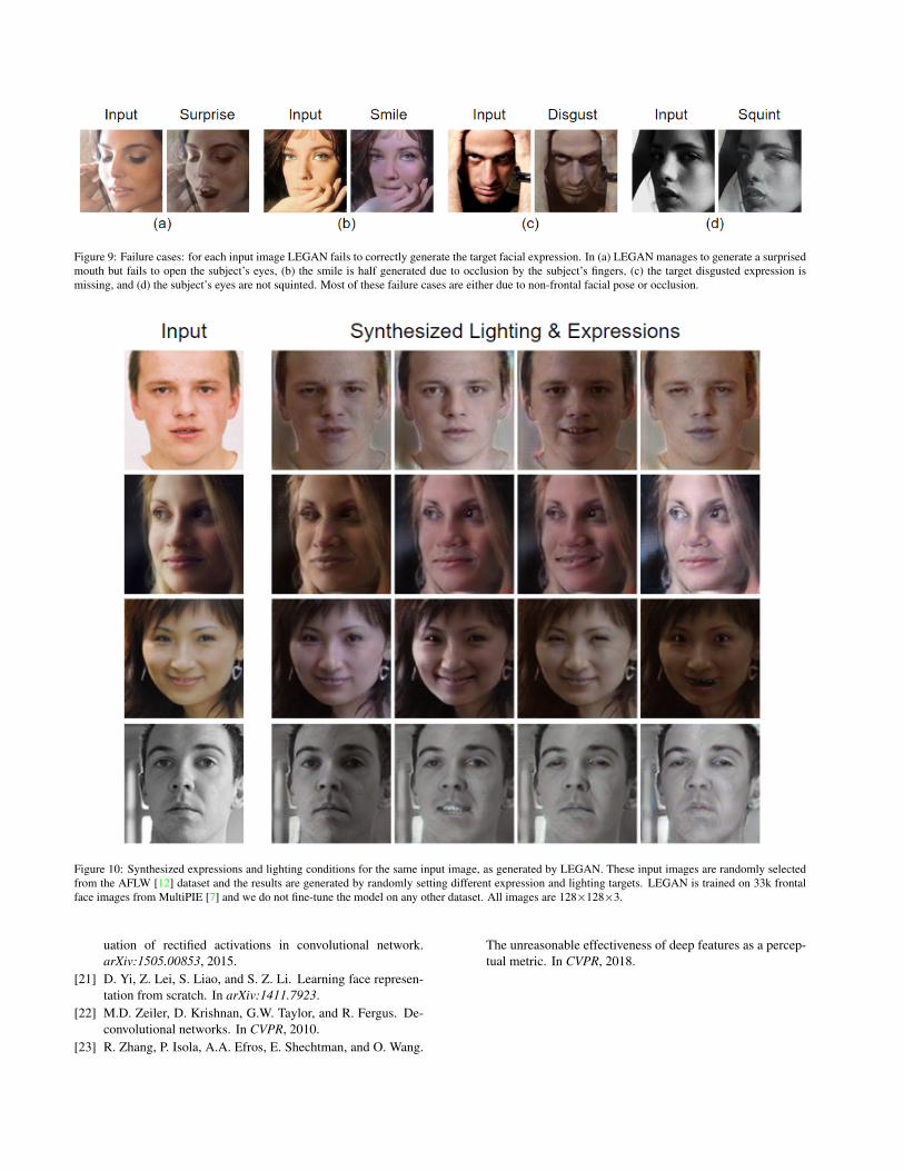
Figure 9: Failure cases: for each input image LEGAN fails to correctly generate the target facial expression. In (a) LEGAN manages to generate a surprisedmouth but fails to open the subject’s eyes, (b) the smile is half generated due to occlusion by the subject’s fingers, (c) the target disgusted expression ismissing, and (d) the subject’s eyes are not squinted. Most of these failure cases are either due to non-frontal facial pose or occlusion.

Figure 10: Synthesized expressions and lighting conditions for the same input image, as generated by LEGAN. These input images are randomly selectedfrom the AFLW [12] dataset and the results are generated by randomly setting different expression and lighting targets. LEGAN is trained on 33k frontalface images from MultiPIE [7] and we do not fine-tune the model on any other dataset. All images are 128×128×3.

uation of rectified activations in convolutional network.arXiv:1505.00853, 2015.

[21] D. Yi, Z. Lei, S. Liao, and S. Z. Li. Learning face represen-tation from scratch. In arXiv:1411.7923.

[22] M.D. Zeiler, D. Krishnan, G.W. Taylor, and R. Fergus. De-convolutional networks. In CVPR, 2010.

[23] R. Zhang, P. Isola, A.A. Efros, E. Shechtman, and O. Wang.

The unreasonable effectiveness of deep features as a percep-tual metric. In CVPR, 2018.

Figure 11: Synthesized expressions and lighting conditions for the same input image, as generated by LEGAN. These input images are randomly selectedfrom the CelebA [13] dataset and the results are generated by randomly setting different expression and lighting targets. LEGAN is trained on 33k frontalface images from MultiPIE [7] and we do not fine-tune the model on any other dataset. All images are 128×128×3.

Figure 12: Recolorization Example: We randomly select a test image fromthe MultiPIE [7] dataset and recolor it using the colorization generatorsnapshots, trained using UMDFaces [5] and FFHQ [10] datasets respec-tively. Although the image is recolored, its lighting is preserved by thecolorization generator.

legan: disentangled manipulation of directional lighting

Documents