leo pekelis february 2nd, 2013, bicoastal datafest,...

1/31/13 Classification And Regression Trees : A Practical Guide for Describing a Dataset (1)

1/27file:///Users/leopekelis/Desktop/13_datafest_cart/13_datafest_cart_talk.html#(1)

Classification And Regression Trees : APractical Guide for Describing a Dataset

Leo Pekelis

February 2nd, 2013, Bicoastal Datafest, Stanford University



What is a Tree?

… ?



What is a Tree?

… ?!



What is a (binary) Decision Tree?



What is a (binary) Decision Tree? Example

The data is all donations to SPACs in excess of $200, by early 2012, from fec.gov



The Structural Model

are subregions of the input variable space, and is a vector of inputvariables.

Examples: ,

are the estimated values of the outcome (y) in region

CART tries to minimize

with respect to and

F(x) = I(x B )KMi=1 cm Rm

{Rm}M1 x

{ < 15.2}x9 {9 <= < 786 & color = red}x300

cm Rm

e(T) =KNi=1 [ − I(x B )]yi KM

m=1 cm Rm2

cm Rm



Some Important Facts about CART

1. The regions are disjoint and rectangular

giving a piecewise constant approximation to the true

2. CART doesn’t find the “best” regions exactly

uses recursive partitioning, or a greedy stepwise descent

3. Both simplifications are to simplify a combinatorally hard problem and make itsolvable in reasonable time.

also allows for natural representations of regions as a binary decision tree

Rm

F(x)



How do we run it?# install the package to Rinstall.packages("rpart", repos = "http://cran.us.r-project.org")

## ## The downloaded binary packages are in## /var/folders/0m/xzr0fktj78sgl36y77z34djr0000gn/T//RtmpPUlWHm/downloaded_packages

# load the librarylibrary(rpart)

# load the datasetload("spac.Rdata")

spac.tree = rpart(Donation ~ ., data = spac.data, cp = 10̂(-6))

#### the function arguments:

# 1) formula, of the form: outcome ~ predictors

# note: outcome ~ . is 'use all other variables in data'

# 2) data: a data.frame object, or any matrix which has variables as# columns and observations as rows

# 3) cp: used to choose depth of the tree, we'll manually prune the tree# later and hence set the threshold very low (more on this later)

# The commands, print() and summary() will be useful to look at the tree.# But first, lets see how big the created tree was

# The object spac.tree is a list with a number of entires that can be# accessed via the $ symbol. A list is like a hash table.

# To see the entries in a list, use names()names(spac.tree)

## [1] "frame" "where" "call" ## [4] "terms" "cptable" "method" ## [7] "parms" "control" "functions" ## [10] "numresp" "splits" "csplit" ## [13] "variable.importance" "y" "ordered"

# Within spac.tree the cptable will tell us a little about the size of the# treespac.tree$cptable[1:10, ]

## CP nsplit rel error xerror xstd## 1 0.037317 0 1.0000 1.000 0.3477## 2 0.016462 2 0.9254 1.078 0.3493## 3 0.003617 6 0.8595 1.068 0.3300## 4 0.002751 8 0.8523 1.051 0.3171## 5 0.001581 9 0.8495 1.050 0.3170## 6 0.001516 17 0.8369 1.064 0.3170## 7 0.001470 21 0.8305 1.064 0.3170## 8 0.001454 27 0.8217 1.066 0.3170## 9 0.001432 29 0.8188 1.066 0.3170## 10 0.001020 32 0.8145 1.069 0.3170

# ...

spac.tree$cptable[dim(spac.tree$cptable)[1] - 9:0, ]

## CP nsplit rel error xerror xstd## 84 1.901e-06 169 0.7951 1.067 0.3133



## 85 1.725e-06 170 0.7951 1.067 0.3133## 86 1.584e-06 171 0.7951 1.067 0.3133## 87 1.188e-06 172 0.7951 1.067 0.3133## 88 1.177e-06 173 0.7951 1.067 0.3133## 89 1.156e-06 174 0.7951 1.067 0.3133## 90 1.135e-06 175 0.7951 1.067 0.3133## 91 1.129e-06 177 0.7951 1.067 0.3133## 92 1.061e-06 179 0.7951 1.067 0.3133## 93 1.000e-06 181 0.7951 1.067 0.3133

# that's a lot of splits! I'm going to prune the tree to 9 splits

cp9 = which(spac.tree$cptable[, 2] == 9)

spac.tree9 = prune(spac.tree, spac.tree$cptable[cp9, 1])

# now lets look at the tree with print() and summary()

print(spac.tree9)

## n= 3668 ## ## node), split, n, deviance, yval## * denotes terminal node## ## 1) root 3668 1.438e+14 30940.0 ## 2) NV=0 3627 9.400e+13 28140.0 ## 4) FID=otherFID,C00487470,C00488403,C00499335 3239 8.088e+13 20110.0 ## 8) smbiz=0 3027 2.897e+13 16380.0 ## 16) blank=0 2467 1.580e+13 10930.0 *## 17) blank=1 560 1.278e+13 40370.0 *## 9) smbiz=1 212 5.126e+13 73400.0 ## 18) TX=0 165 1.867e+12 26050.0 *## 19) TX=1 47 4.772e+13 239600.0 ## 38) FID=C00488403,C00499335 31 5.142e+06 567.2 *## 39) FID=otherFID 16 4.252e+13 702800.0 *## 5) FID=C00490045 388 1.117e+13 95130.0 ## 10) NY=0 345 6.533e+12 82900.0 *## 11) NY=1 43 4.176e+12 193300.0 ## 22) Day< 27.5 35 2.033e+12 138000.0 *## 23) Day>=27.5 8 1.568e+12 435000.0 *## 3) NV=1 41 4.723e+13 278400.0 ## 6) Month>=3 32 3.476e+11 41390.0 *## 7) Month< 3 9 3.869e+13 1121000.0 *

summary(spac.tree9)

## Call:## rpart(formula = Donation ~ ., data = spac.data, cp = 10̂(-6))## n= 3668 ## ## CP nsplit rel error xerror xstd## 1 0.037317 0 1.0000 1.000 0.3477## 2 0.016462 2 0.9254 1.078 0.3493## 3 0.003617 6 0.8595 1.068 0.3300## 4 0.002751 8 0.8523 1.051 0.3171## 5 0.001581 9 0.8495 1.050 0.3170## ## Variable importance## Month FID NV TX tech oil doctor writing smbiz ## 35 28 9 6 3 3 3 3 2 ## Day NY blank biz ## 2 2 1 1 ## ## Node number 1: 3668 observations, complexity param=0.03732## mean=3.094e+04, MSE=3.919e+10 ## left son=2 (3627 obs) right son=3 (41 obs)## Primary splits:## NV splits as LR, improve=0.017660, (0 missing)## FID splits as LRLLL, improve=0.012390, (0 missing)## Month < 5.5 to the right, improve=0.005567, (0 missing)



## smbiz splits as LR, improve=0.004716, (0 missing)## retired splits as RL, improve=0.003653, (0 missing)## ## Node number 2: 3627 observations, complexity param=0.01646## mean=2.814e+04, MSE=2.592e+10 ## left son=4 (3239 obs) right son=5 (388 obs)## Primary splits:## FID splits as LRLLL, improve=0.020740, (0 missing)## smbiz splits as LR, improve=0.008136, (0 missing)## money splits as LR, improve=0.004718, (0 missing)## retired splits as RL, improve=0.004439, (0 missing)## Month < 6.5 to the right, improve=0.004148, (0 missing)## Surrogate splits:## UT splits as LR, agree=0.897, adj=0.036, (0 split)## leisure splits as LR, agree=0.893, adj=0.003, (0 split)## ## Node number 3: 41 observations, complexity param=0.03732## mean=2.784e+05, MSE=1.152e+12 ## left son=6 (32 obs) right son=7 (9 obs)## Primary splits:## Month < 3 to the right, improve=0.17340, (0 missing)## Day < 7.5 to the right, improve=0.02769, (0 missing)## manage splits as LR, improve=0.02717, (0 missing)## FID splits as RL--L, improve=0.02251, (0 missing)## professional splits as RL, improve=0.01382, (0 missing)## Surrogate splits:## doctor splits as LR, agree=0.805, adj=0.111, (0 split)## tech splits as LR, agree=0.805, adj=0.111, (0 split)## oil splits as LR, agree=0.805, adj=0.111, (0 split)## writing splits as LR, agree=0.805, adj=0.111, (0 split)## ## Node number 4: 3239 observations, complexity param=0.01646## mean=2.011e+04, MSE=2.497e+10 ## left son=8 (3027 obs) right son=9 (212 obs)## Primary splits:## smbiz splits as LR, improve=0.007964, (0 missing)## FID splits as R-LLL, improve=0.005066, (0 missing)## blank splits as LR, improve=0.003437, (0 missing)## TX splits as LR, improve=0.002374, (0 missing)## retired splits as RL, improve=0.002351, (0 missing)## ## Node number 5: 388 observations, complexity param=0.003617## mean=9.513e+04, MSE=2.88e+10 ## left son=10 (345 obs) right son=11 (43 obs)## Primary splits:## NY splits as LR, improve=0.041680, (0 missing)## Day < 27.5 to the left, improve=0.028980, (0 missing)## CA splits as RL, improve=0.023540, (0 missing)## retired splits as RL, improve=0.011260, (0 missing)## Month < 1.5 to the left, improve=0.007873, (0 missing)## Surrogate splits:## community splits as LR, agree=0.892, adj=0.023, (0 split)## ## Node number 6: 32 observations## mean=4.139e+04, MSE=1.086e+10 ## ## Node number 7: 9 observations## mean=1.121e+06, MSE=4.299e+12 ## ## Node number 8: 3027 observations, complexity param=0.002751## mean=1.638e+04, MSE=9.572e+09 ## left son=16 (2467 obs) right son=17 (560 obs)## Primary splits:## blank splits as LR, improve=0.013650, (0 missing)## FID splits as R-LLL, improve=0.007902, (0 missing)## DC splits as LR, improve=0.007561, (0 missing)## retired splits as RL, improve=0.003920, (0 missing)## Day < 14.5 to the left, improve=0.002814, (0 missing)## Surrogate splits:## DC splits as LR, agree=0.870, adj=0.300, (0 split)## ZZ splits as LR, agree=0.815, adj=0.002, (0 split)## ## Node number 9: 212 observations, complexity param=0.01646## mean=7.34e+04, MSE=2.418e+11



## left son=18 (165 obs) right son=19 (47 obs)## Primary splits:## TX splits as LR, improve=0.032550, (0 missing)## Month < 1.5 to the right, improve=0.017010, (0 missing)## FID splits as R-LLL, improve=0.009249, (0 missing)## Day < 28.5 to the left, improve=0.007682, (0 missing)## professional splits as RL, improve=0.002284, (0 missing)## Surrogate splits:## FID splits as L-LRL, agree=0.892, adj=0.511, (0 split)## teach splits as LR, agree=0.783, adj=0.021, (0 split)## oil splits as LR, agree=0.783, adj=0.021, (0 split)## ## Node number 10: 345 observations## mean=8.29e+04, MSE=1.894e+10 ## ## Node number 11: 43 observations, complexity param=0.003617## mean=1.933e+05, MSE=9.711e+10 ## left son=22 (35 obs) right son=23 (8 obs)## Primary splits:## Day < 27.5 to the left, improve=0.137500, (0 missing)## Month < 5 to the right, improve=0.062300, (0 missing)## money splits as LR, improve=0.012980, (0 missing)## professional splits as RL, improve=0.010520, (0 missing)## manage splits as LR, improve=0.009981, (0 missing)## Surrogate splits:## tech splits as LR, agree=0.837, adj=0.125, (0 split)## ## Node number 16: 2467 observations## mean=1.093e+04, MSE=6.405e+09 ## ## Node number 17: 560 observations## mean=4.037e+04, MSE=2.282e+10 ## ## Node number 18: 165 observations## mean=2.605e+04, MSE=1.131e+10 ## ## Node number 19: 47 observations, complexity param=0.01646## mean=2.396e+05, MSE=1.015e+12 ## left son=38 (31 obs) right son=39 (16 obs)## Primary splits:## FID splits as R--LL, improve=0.109000, (0 missing)## Day < 28.5 to the left, improve=0.043090, (0 missing)## Month < 5 to the right, improve=0.038900, (0 missing)## manage splits as RL, improve=0.005604, (0 missing)## Surrogate splits:## Month < 3.5 to the right, agree=0.787, adj=0.375, (0 split)## biz splits as LR, agree=0.681, adj=0.063, (0 split)## ## Node number 22: 35 observations## mean=1.38e+05, MSE=5.809e+10 ## ## Node number 23: 8 observations## mean=4.35e+05, MSE=1.961e+11 ## ## Node number 38: 31 observations## mean=567.2, MSE=1.659e+05 ## ## Node number 39: 16 observations## mean=7.028e+05, MSE=2.658e+12 ##

# finally, lets get a graphical representation of the tree, and save to a# png filepng("spactree9.png", width = 1200, height = 800)post(spac.tree9, file = "", title. = "Classifying SPAC Donation Size, 9 splits", bp = 18)dev.off()

## pdf ## 2



How do we run it? The graphicalrepresentation.



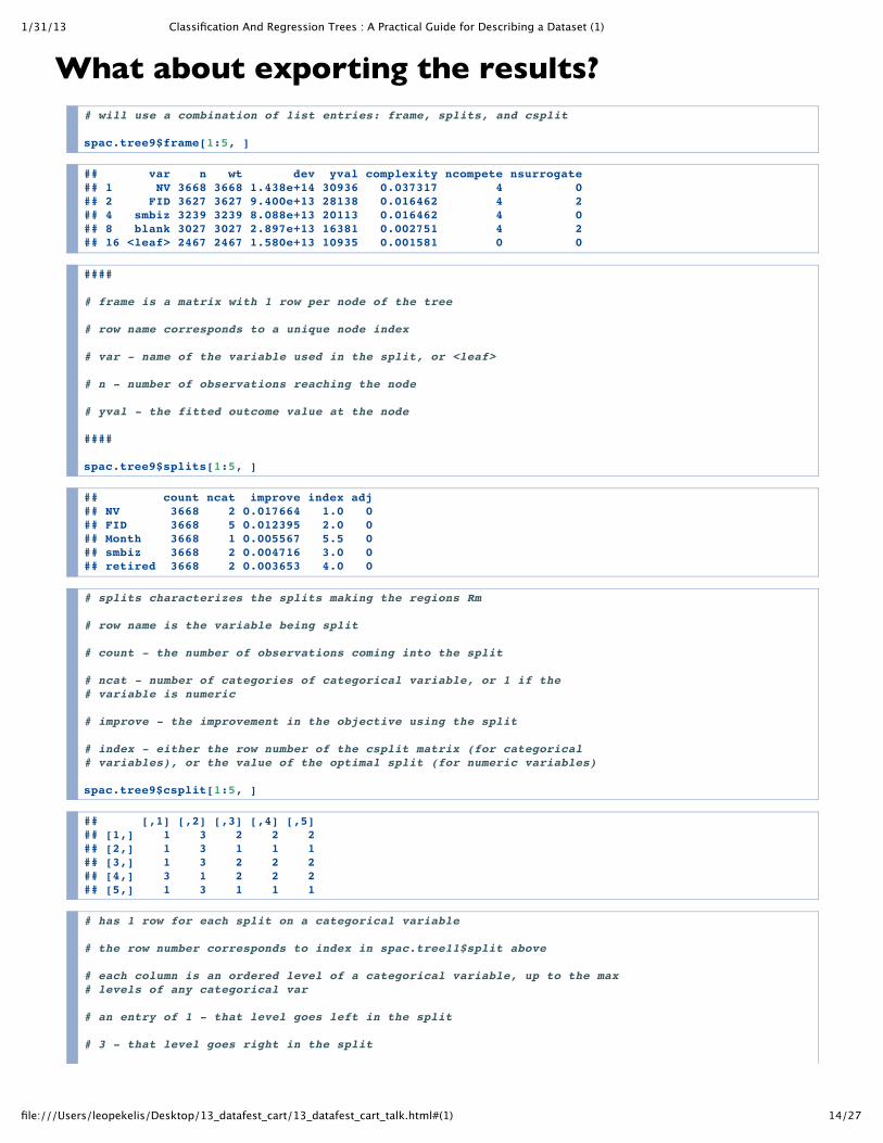
What about exporting the results?# will use a combination of list entries: frame, splits, and csplit

spac.tree9$frame[1:5, ]

## var n wt dev yval complexity ncompete nsurrogate## 1 NV 3668 3668 1.438e+14 30936 0.037317 4 0## 2 FID 3627 3627 9.400e+13 28138 0.016462 4 2## 4 smbiz 3239 3239 8.088e+13 20113 0.016462 4 0## 8 blank 3027 3027 2.897e+13 16381 0.002751 4 2## 16 <leaf> 2467 2467 1.580e+13 10935 0.001581 0 0

####

# frame is a matrix with 1 row per node of the tree

# row name corresponds to a unique node index

# var - name of the variable used in the split, or <leaf>

# n - number of observations reaching the node

# yval - the fitted outcome value at the node

####

spac.tree9$splits[1:5, ]

## count ncat improve index adj## NV 3668 2 0.017664 1.0 0## FID 3668 5 0.012395 2.0 0## Month 3668 1 0.005567 5.5 0## smbiz 3668 2 0.004716 3.0 0## retired 3668 2 0.003653 4.0 0

# splits characterizes the splits making the regions Rm

# row name is the variable being split

# count - the number of observations coming into the split

# ncat - number of categories of categorical variable, or 1 if the# variable is numeric

# improve - the improvement in the objective using the split

# index - either the row number of the csplit matrix (for categorical# variables), or the value of the optimal split (for numeric variables)

spac.tree9$csplit[1:5, ]

## [,1] [,2] [,3] [,4] [,5]## [1,] 1 3 2 2 2## [2,] 1 3 1 1 1## [3,] 1 3 2 2 2## [4,] 3 1 2 2 2## [5,] 1 3 1 1 1

# has 1 row for each split on a categorical variable

# the row number corresponds to index in spac.tree11$split above

# each column is an ordered level of a categorical variable, up to the max# levels of any categorical var

# an entry of 1 - that level goes left in the split

# 3 - that level goes right in the split



# 2 - that level is not included in the split



What about exporting the results?

To recreate a decision tree, you would at least extract the following columns ofinformation:

rownames(spac.tree9$splits)

spac.tree9$splits[,"count"], spac.tree9$splits[,"index"] and

spac.tree9$splits[,"ncat"]

spac.tree9$frame[,"var"], spac.tree9$[,"n"] and

spac.tree9$frame[,"yval"]

spac.tree9$csplit corresponding to the rows given by "index" where "ncat" > 2in "splits"

The order of splits in "frame" are depth first, and left branch first

Match between "frame" and "splits" by variable name and number ofobservations

since a variable can be split multiple times, and frame also includes competing and surrogate splits



Automatic Way to Select Tree Size

Can calculate contribution of split to decreasing objective by

If then accept the split, otherwise make a terminal node

is a tuning parameter, giving tree sizes as in “cptable”

Actually a little trickier because the rule is applied in inverse order of depth

Solves the problem:

where is the number of terminal nodes of the tree

e(T)

= ( −em1N K Bxi Rm

yi y!m)2

Im = − −pm em eml emr

Im ¦ cppm m

cp > 0

[e(T) + cp|T |]minT

|T |



Automatic Way to Select Tree Size

The entry "cptable" gives tree statistics for each

"rel error" is the ratio of the objective, , to that of a single root tree

This is always decreasing with

"xerror" is the average of 10 fold cross validation error

i.e. leave out 1/10th of the dataset,

train a size n tree on the other 9/10ths,

and compute on the left out part

this is more useful for prediction, and not as useful to us for describing a dataset

can be thought of as a measure of pervasiveness

Could consider a criteria that penalizes large trees

Not unreasonable:

cp

e(T)

cp

e(T)

N × (relerror) + 2|T |



Automatic Way to Select Tree Sizewhich.min(spac.tree$cptable[, 4])

## 1 ## 1

# gives a value of 1, meaning none of the splits are 'pervasize'

# but using the criteria above, penalizing large treescpstat = dim(spac.data)[1] * spac.tree$cptable[, 3] + 2 * (spac.tree$cptable[, 2] + 1)

round(spac.tree$cptable[which.min(cpstat), ], 3)

## CP nsplit rel error xerror xstd ## 0.001 39.000 0.808 1.064 0.313

# suggests a tree size with 39 splits



Advantages of Trees

1. Fast computations

2. Invariant under monotone transformations of variables

Scaling doesn’t matter!

Immune to outliers in x

3. Resistence to irrelevant variables, so can throw lots of variables into it

4. One tuning parameter (tree size, or cp)

5. Interpretable model representation

6. Handles missing data by keeping track of surrogate, or highly correlated,backup splits at every node

7. Extends to categorical outcomes easily



Disadvantages of Trees

1. Accuracy

may not be piecewise constant (but decent overall approximation)

Data Fragmentation (ok, if you have lots of data)

must involve high order interactions

2. Variance

Each subsequent split depends on the previous ones, so an error in a higher split is propogateddown.

Small change in dataset can cause big change in tree

If you only have a random sample of a population, this can be a problem.

Not as much of an issue if you’re describing a dataset

F(x)

F(x)



CART libraries outside of R: weka

weka 3: Data mining software in JAVA

http://www.cs.waikato.ac.nz/ml/weka/

Relevent class weka.classifiers.trees.J48

Simple command line syntax

java weka.classifiers.trees.J48 -t data/weather.arff -i

ARFF is Attribute-Relation File Format and data format for weka

weka.core.converters package contains converters for usual data files

Also call classes directly

import weka.core.Instances; import weka.classifiers.Evaluation; import weka.classifiers.trees.J48; … Instances train = … // from somewhere Instances test = … // from somewhere // train classifier Classifier cls = new J48(); cls.buildClassifier(train); // evaluate classifier and print some statistics Evaluation eval = new Evaluation(train); eval.evaluateModel(cls, test); System.out.println(eval.toSummaryString(“”, false));

weka.gui.treevisualizer.TreeVisualizer class to vizualize trees

http://www.cs.waikato.ac.nz/ml/weka/



CART libraries outside of R: orange

orange: Data mining through visual programming programming or Python scripting.

http://orange.biolab.si/

has proprietary tab-deliminated data format

Can import from csv, but is not very robust

More info: /Orange.data.formats/

Relevant function: Orange.regression.tree.TreeLearner(...)

Vizualizing trees: Orange renders trees in dot - plain text graph descriptionlangauge readable by both human and computer

tree.dot(file_name="0.dot", node_shape="ellipse",leaf_shape="box")

http://orange.biolab.si/

http://orange.biolab.si/docs/latest/reference/rst/Orange.data.formats/



CART libraries outside of R: opencv

opencv: (Open Source Computer Vision) is a library of programming functions forreal time computer vision, in C++

http://opencv.willowgarage.com/wiki/

Uses n-dimensional array class Mat to store and operate on data

core_basic_structures.html#mat

CvDTree class is an honest representation of CART algorithm

ml_decision_trees.html

mushroom.cpp example file demonstrates how to use decision trees

http://opencv.willowgarage.com/wiki/

http://opencv.willowgarage.com/documentation/cpp/core_basic_structures.html#mat

http://opencv.willowgarage.com/documentation/cpp/ml_decision_trees.html



References

Elements of Statistical Learning. 2009. New York. Springer. xxii, 745 p. : ill. ; 24 cm.

Jerome Friedman’s 315b course notes

http://www-stat.stanford.edu/~tibs/ElemStatLearn/

http://www-stat.stanford.edu/~owen/courses/321/readings/CV-SVD-JSM.pdf



Two solutions to Disadvantages (extraslides)

1. Boosted Trees, aka Forests, MART

Now each is a tree, and is a linear combination of trees

Each tree can model an additive effect, or many low order interactions

Variance of a combination of identically distributed objects is lower than any individual

Disadvantage: loses decision tree interpretability unless K is small

2. Random Forests

Similar to boosted trees, but now random subsets of the data are used for each tree

Simpler to fit than boosted trees

Accuracy is usually somewhere in between a single tree and boosted trees

F(x) = f (x ; , )KKk=1 ak ck

m Rkm

f () F()



How are Boosted Trees Interpreted? (extraslides)

Relative Importance

Average overall improvement of objective by variable

Partial Dependence

Predicted outcome using , after averaging out the others

Im = Avg[ Im I(var(m) = l)]p2l KM

m=1 pm

l

pd( ) = [F( , )]xl Enotl xl xnotl

xl

leo pekelis february 2nd, 2013, bicoastal datafest,...

Documents