lethbridge complex analysis - university of lethbridge
TRANSCRIPT

LethbridgeComplexAnalysisLecture Notes
Dave Witte MorrisUniversity of Lethbridge, Canada
http://people.uleth.ca/∼∼∼dave.morris/
Version 0.50 of September 7, 2021
To the extent possible under law, Dave Witte Morris has waivedall copyright and related or neighbouring rights to this work.
You can copy, modify, and distribute this work, even for commercial purposes, all without asking permission. Formore information, visit http://creativecommons.org/publicdomain/zero/1.0/


Contents
Chapter 1. Complex Numbers 11.1. Introduction to complex numbers 1
§1.1A. Elementary properties of complex numbers 1§1.1B. Exponential function, sine, and cosine 4§1.1C. Rectangular form and polar form 6§1.1D. Roots of unity 9§1.1E. Complex conjugate and division 9
1.2. Graphs of complex functions 101.3. Basic concepts of topology 12
§1.3A. Open sets 12§1.3B. Triangle inequality 14§1.3C. Paths 15§1.3D. Connected sets 16
1.4. Functions as mappings 181.5. Branch cuts 20
Chapter 2. Limits, Continuity, and Derivatives 232.1. Limits 232.2. Continuity 252.3. Derivatives 26
§2.3A. Differentiation 26§2.3B. Holomorphic functions and poles 29§2.3C. Derivative of ez and trigonometric functions 30
2.4. Cauchy-Riemann equations 312.5. Harmonic functions 342.6. The official definition of a limit 37
Chapter 3. Integration 413.1. Contour integrals 413.2. Cauchy-Goursat Theorem 463.3. Deformation of Contours 483.4. Antiderivatives 503.5. Cauchy Integral Formula 533.6. Cauchy Integral Formula for Derivatives 563.7. Consequences of the Cauchy Integral Formulas 60
3

4 CONTENTS
Chapter 4. Power Series 654.1. Review of sequences and series 65
§4.1A. Sequences 65§4.1B. Order of magnitude 65§4.1C. Series 68
4.2. Power series 704.3. Power series and holomorphic functions 724.4. Multiplicity of zeros 74
Chapter 5. Residue Theorem 775.1. Laurent series 775.2. Classification of singularities 795.3. Residue Theorem 815.4. Using the Residue Theorem to Calculate Real Integrals 84
Index of Definitions 91

CHAPTER 1
Complex Numbers
1.1. Introduction to complex numbersThis is a course about several topics that you should have encountered in your calculus courses,
such as integration, differentiation, continuity, limits, and power series. However, instead of usingonly the usual “real” numbers (that is, numbers that are either positive, negative, or zero), we willallow more general “complex” numbers. Before we start doing calculus (in the next chapter), wewill spend some time getting comfortable with complex numbers.
§1.1A. Elementary properties of complex numbers.
(1.1.1) Recall. The numbers that arose in (most of?) your previous math classes were eitherpositive, negative, or zero, so they can be drawn on the number line:
-3 -2 -1 0 1 2 3
e√
2 π−12 loge 10
These are called real numbers, and the set of these numbers is denoted R. Some important subsetsof R are:
• The set Z = {0,±1,±2,±3, . . .} of all integers.• The set Z+ = {1, 2, 3, . . .} of all positive integers.• The set N = Z+ ∪ {0} = {0, 1, 2, 3, . . .} of all natural numbers.• The set Q = {m/n | m,n ∈ Z, n = 0 } of all rational numbers (or fractions).
We have Z+ ⊂ N ⊂ Z ⊂ Q ⊂ R. In addition to all of the rational numbers, the set R also containsirrational numbers, such as
√2 = 1.41421 . . . , π = 3.14159 . . . , e = 2.71828 . . . , loge 10 = 2.30258 . . .
and many others. (Every real number can be represented as a decimal, which may be infinitelylong.)
It is a basic fact that every real number is either positive, negative, or zero. Therefore:
(1.1.2) Exercise. Show that if x is any real number, then x2 ≥ 0.[Hint. positive × positive = positive, negative × negative = positive, 0 × 0 = 0.]
So, you were probably taught: “You can’t take the square root of a negative number.” But thatwill not be the case in this course: we assume that −1 has a square root, and this square root willbe called i:
i =√−1, so i2 = −1 .
It is obvious (from Exercise 1.1.2) that i is not a real number. Mathematicians call it an “imaginary”number. By using imaginary numbers, we will see in Exercise 1.1.39(2) that we can take the squareroot of any number, even the negative ones.
1

2 1. COMPLEX NUMBERS
(1.1.3) Note. We havei0 = 1,
i1 = i,
i2 = −1,
i3 = i2 · i = −1 · i = −i,
i4 = i3 · i = −i · i = −i2 = −(−1) = 1.
At this point, since i4 = 1 = i0, we are back to where we started, so the same values will repeatover and over (1, i,−1,−i, 1, i,−1,−i, . . .), as summarized in the following table:
k 0 1 2 3 4 5 6 7 8 9 · · ·ik 1 i −1 −i 1 i −1 −i 1 i · · ·
Thus, ik only depends on the remainder when you divide k by 4. That is, if k ≡ ℓ (mod 4),then ik = iℓ. (This is similar to the fact that (−1)k only depends on whether k is even or odd.)Therefore, it is easy to raise i to any power, even a large one. For example,
i103 = i100 · i3 = 1 · (−i) = −i.
So you should remember (or be sure you can quickly figure out) the values of ik for k = 1, 2, 3, 4.
(1.1.4) Definition.• A complex number is an expression of the form x + yi, where x and y are real numbers.• Complex numbers are added, subtracted, and multiplied by using the basic laws of algebra
that you learned in high school (and before), with the additional rule that i2 = −1. (SeeRemark 1.1.48 for an explanation of how to divide two complex numbers.)
• The set of all complex numbers is denoted C.
(1.1.5) Terminology.• The real part of x + yi is x, and the imaginary part is y (if x and y are real numbers).
They are denoted Re z and Im z, respectively, soz = (Re z) + (Im z)i.
Note: the real and imaginary parts are real numbers — do not include i in Im z.• Any complex number whose real part is 0 (i.e., any number of the form yi, where y is a real
number) is called an imaginary number.
(1.1.6) Example. We have:(3 + 5i) + (6 − 11i) = (3 + 6) + (5 − 11)i = 9 − 6i
and(3 + 5i)(6 − 11i) = (3)(6) + (3)(−11i) + (5i)(6) + (5i)(−11i) (FOIL)
= 18 − 33i + 30i − 55i2
= 18 − 3i − 55(−1) (i2 = −1)= 73 − 3i.
(1.1.7) Remark. In general:(1) The formula for the sum of two complex numbers is:
(x1 + y1i) + (x2 + y2i) = (x1 + x2) + (y1 + y2)i.(2) The formula for the difference of two complex numbers is:
(x1 + y1i) − (x2 + y2i) = (x1 − x2) + (y1 − y2)i.

1.1. INTRODUCTION TO COMPLEX NUMBERS 3
(3) The formula for the product of two complex numbers is:(x1 + y1i)(x2 + y2i) = (x1x2 − y1y2) + (x1y2 + y1x2)i.
(1.1.8) Notation. In high school, the usual variables are x and y. We will continue to use theseletters, but only for real numbers. The usual name for a complex number is z (also z0, z1, z2, . . .),but we will also often use w, when we need to talk about another complex number and do not wantto use subscripts. The letters a, b, and c will be used to denote constants, which may be either realor complex, depending on the context.(1.1.9) Facts.
(1) Complex numbers obey the basic rules of arithmetic:(a) Addition and multiplication are commutative:
z1 + z2 = z2 + z1 and z1z2 = z2z1.
(b) Addition and multiplication are associative:(z1 + z2) + z3 = z1 + (z2 + z3) and (z1z2)z3 = z1(z2z3).
(c) Multiplication distributes over addition:z1(z2 + z3) = z1z2 + z1z3 and (z1 + z2)z3 = z1z3 + z2z3.
(d) If a product is zero, then one of the factors must be zero:If z1z2 = 0, then either z1 = 0 or z2 = 0.
(e) 0 + z = z + 0 = z, 1 · z = z · 1 = z, and 0 · z = z · 0 = 0.(2) Two complex numbers z1 = x1 + y1i and z2 = x2 + y2i are equal iff x1 = x2 and y1 = y2.
(1.1.10) Exercise. Verify Fact 1.1.9(1), except (1d). (Part (1d) will be easier after we have a bitof theory, so its verification is postponed to Exercise 1.1.39(6).)(1.1.11) Warning. There are (at least) two major differences between complex numbers and realnumbers:
(1) The square of a complex number can be negative. (For example, i2 = −1 < 0.) In otherwords, negative numbers can have square roots. In fact, we will see in Exercise 1.1.39(2) thatevery complex number has a square root.
(2) If you have two real numbers x and y, then either x < y or x > y (or x = y). In particular,as we have already said, every real number is either positive (i.e., > 0) or negative (i.e., < 0)or zero (i.e., = 0). But there is no natural way to compare complex numbers in this way: wenever write “z1 < z2” or “z1 > z2” unless z1 and z2 are real numbers.
(1.1.12) Exercise. Let z1 = 2 + 3i and z2 = 4 − 5i. Calculate each of the following:(1) 6z1 − 3z2
(2) z1 + iz2,(3) z2
1 ,(4) z1z2,
(5) z31 ,
(6) f(z1), for f(z) = 2z2−5z.
You need to be able to do algebra with complex numbers:(1.1.13) Example. Find all of the square roots of 7 + 24i.
Solution. Suppose z2 = 7 + 24i, and write z = x + yi (with x, y ∈ R). Then7 + 24i = z2 = (x + yi)2 = x2 + 2xyi + y2i2 = x2 + 2xyi + y2(−1) = (x2 − y2) + 2xyi,
so (by Fact 1.1.9(2))
7 = x2 − y2 and 24 = 2xy.
From the second equation, we see that
y =242x
=12x
.
4 1. COMPLEX NUMBERS
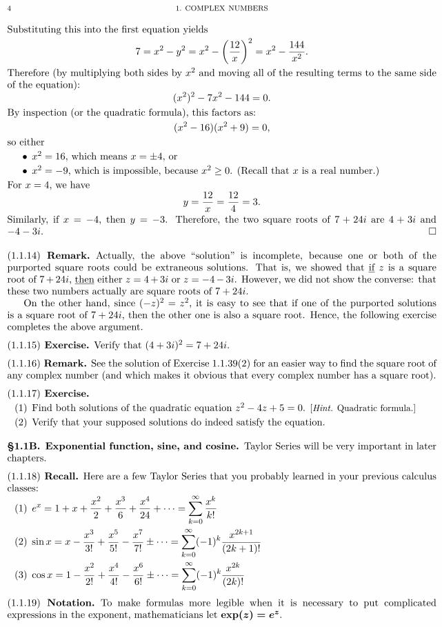
Substituting this into the first equation yields
7 = x2 − y2 = x2 −(
12x
)2
= x2 − 144x2
.
Therefore (by multiplying both sides by x2 and moving all of the resulting terms to the same sideof the equation):
(x2)2 − 7x2 − 144 = 0.
By inspection (or the quadratic formula), this factors as:(x2 − 16)(x2 + 9) = 0,
so either• x2 = 16, which means x = ±4, or• x2 = −9, which is impossible, because x2 ≥ 0. (Recall that x is a real number.)
For x = 4, we havey =
12x
=124
= 3.
Similarly, if x = −4, then y = −3. Therefore, the two square roots of 7 + 24i are 4 + 3i and−4 − 3i. □
(1.1.14) Remark. Actually, the above “solution” is incomplete, because one or both of thepurported square roots could be extraneous solutions. That is, we showed that if z is a squareroot of 7+24i, then either z = 4+3i or z = −4− 3i. However, we did not show the converse: thatthese two numbers actually are square roots of 7 + 24i.
On the other hand, since (−z)2 = z2, it is easy to see that if one of the purported solutionsis a square root of 7 + 24i, then the other one is also a square root. Hence, the following exercisecompletes the above argument.
(1.1.15) Exercise. Verify that (4 + 3i)2 = 7 + 24i.
(1.1.16) Remark. See the solution of Exercise 1.1.39(2) for an easier way to find the square root ofany complex number (and which makes it obvious that every complex number has a square root).
(1.1.17) Exercise.(1) Find both solutions of the quadratic equation z2 − 4z + 5 = 0. [Hint. Quadratic formula.](2) Verify that your supposed solutions do indeed satisfy the equation.
§1.1B. Exponential function, sine, and cosine. Taylor Series will be very important in laterchapters.
(1.1.18) Recall. Here are a few Taylor Series that you probably learned in your previous calculusclasses:
(1) ex = 1 + x +x2
2+
x3
6+
x4
24+ · · · =
∞∑k=0
xk
k!
(2) sin x = x − x3
3!+
x5
5!− x7
7!± · · · =
∞∑k=0
(−1)k x2k+1
(2k + 1)!
(3) cos x = 1 − x2
2!+
x4
4!− x6
6!± · · · =
∞∑k=0
(−1)k x2k
(2k)!
(1.1.19) Notation. To make formulas more legible when it is necessary to put complicatedexpressions in the exponent, mathematicians let exp(z) = ez.

1.1. INTRODUCTION TO COMPLEX NUMBERS 5
In this course, we will use these same formulas, but we will replace the real number x with acomplex number z = x + yi. (All three of these series converge for all values of z, as will be seenin Exercise 4.2.3.)
(1.1.20) Note. If we write z = x + yi, then we haveez = ex+yi = ex eyi = ex eiy
and
eiy = 1 + (iy) +(iy)2
2!+
(iy)3
3!+
(iy)4
4!+
(iy)5
5!+
(iy)6
6!+ · · ·
= 1 + iy + i2y2
2!+ i3
y3
3!+ i4
y4
4!+ i5
y5
5!+ i6
y6
6!+ · · ·
= 1 + iy − y2
2!− i
y3
3!+
y4
4!+ i
y5
5!− y6
6!± · · · (see Note 1.1.3)
=(
1 − y2
2!+
y4
4!− y6
6!± · · ·
)+ i
(y − y3
3!+
y5
5!− y7
7!± · · ·
)= cos y + i sin y.
Putting these together yields:(1.1.21) ex+yi = ex(cos y + i sin y).
Many textbooks define ez by using this formula, instead of the Taylor series. (And you are welcometo do so, if you prefer.)
The case x = 0 of this formula is very important (and is usually stated with θ in the place of y):
(1.1.22) Lemma (Euler’s formula).
eiθ = cos θ + i sin θ
(1.1.23) Exercise. Calculate each of the following:(1) eiπ,(2) e−iπ,
(3) eiπ/2,(4) e−iπ/2,
(5) e2πi,(6) e100πi,
(7) e1+3πi.(8) exp(log 3 + πi).
Note: All logarithms in this textbook are to base e.
Several important trig identities can easily be derived from Euler’s formula. (Thus, there is noneed to memorize these identities, if you know how to use Euler’s formula.)
(1.1.24) Example. Derive the double-angle formulas for cosine and sine.
Solution. We havecos 2θ + i sin 2θ = e2iθ (Euler’s Formula)
= (eiθ)2
= (cos θ + i sin θ)2 (Euler’s Formula)= cos2 θ + 2i sin θ cos θ + (i sin θ)2
= (cos2 θ − sin2 θ) + 2i sin θ cos θ (i2 = −1).
Thereforecos 2θ = cos2 θ − sin2 θ and sin 2θ = 2 sin θ cos θ. □

6 1. COMPLEX NUMBERS
(1.1.25) Remark. Euler’s formula yields formulas for sin nθ and cos nθ for any integer n, but theyget messy when n is large. For example,
sin 9θ = 9 cos8 θ sin θ − 84 cos6 θ sin3 θ + 126 cos4 θ sin5 θ − 36 cos2 θ sin7 θ + sin9 θ.
(1.1.26) Exercise. Use Euler’s formula to derive:(1) the addition formulas for sine and cosine. (That is, find formulas for sin(a+ b) and cos(a+ b)
that involve only sin a, sin b, cos a, and cos b.)(2) the triple angle formulas for sine and cosine. (That is, find formulas for sin 3θ and cos 3θ that
involve only sin θ and cos θ.)(3) de Moivre’s formula: (cos θ + i sin θ)n = cos nθ + i sin nθ, for θ ∈ R and n ∈ Z+.
(1.1.27) Note. The calculation in Note 1.1.20 shows that the formula eiθ = cos θ + i sin θ is valideven when we replace θ with a complex number z:
eiz = cos z + i sin z.
Since all of the exponents in the power series for sin z are odd, and all of the exponents in thepower series for cos z are even, we have sin(−z) = − sin z and cos(−z) = cos z. Therefore
e−iz = cos z − i sin z.
Now, adding these two equations yieldseiz + e−iz = (cos z + i sin z) + (cos z − i sin z) = 2 cos z,
so
cos z =eiz + e−iz
2.
Similarly, subtracting the two equations yields
sin z =eiz − e−iz
2i.
Many textbooks take these formulas to be the definitions of sin z and cos z, instead of using powerseries.
§1.1C. Rectangular form and polar form. We draw real numbers on the number line, butcomplex numbers are drawn in the complex plane:
• The complex number x + iy can be represented as the point (or vector) (x, y) in thexy-plane R2.
• The x-axis is often referred to as the real axis, because points on the x-axis in R2 correspondto real numbers in C. Similarly, the y-axis is often referred to as the imaginary axis, becausepoints on the y-axis in R2 correspond to imaginary numbers in C.
(1.1.28) Note. In this geometric representation of complex numbers, addition is performed by theusual parallelogram law for addition of vectors.
0
z1
z2
z1 + z2
The geometric description of multiplication is easier to describe in “polar coordinates,” whichuse the variables r and θ.
1.1. INTRODUCTION TO COMPLEX NUMBERS 7
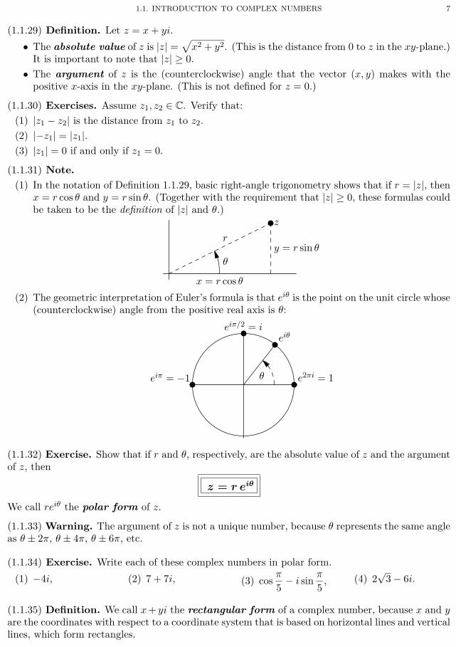
(1.1.29) Definition. Let z = x + yi.• The absolute value of z is |z| =
√x2 + y2. (This is the distance from 0 to z in the xy-plane.)
It is important to note that |z| ≥ 0.• The argument of z is the (counterclockwise) angle that the vector (x, y) makes with the
positive x-axis in the xy-plane. (This is not defined for z = 0.)
(1.1.30) Exercises. Assume z1, z2 ∈ C. Verify that:(1) |z1 − z2| is the distance from z1 to z2.(2) |−z1| = |z1|.(3) |z1| = 0 if and only if z1 = 0.
(1.1.31) Note.(1) In the notation of Definition 1.1.29, basic right-angle trigonometry shows that if r = |z|, then
x = r cos θ and y = r sin θ. (Together with the requirement that |z| ≥ 0, these formulas couldbe taken to be the definition of |z| and θ.)
z
x = r cos θ
y = r sin θr
θ
(2) The geometric interpretation of Euler’s formula is that eiθ is the point on the unit circle whose(counterclockwise) angle from the positive real axis is θ:
eiθ
θ
eiπ/2 = i
eiπ = −1 e2πi = 1
(1.1.32) Exercise. Show that if r and θ, respectively, are the absolute value of z and the argumentof z, then
z = r eiθ
We call reiθ the polar form of z.
(1.1.33) Warning. The argument of z is not a unique number, because θ represents the same angleas θ ± 2π, θ ± 4π, θ ± 6π, etc.
(1.1.34) Exercise. Write each of these complex numbers in polar form.(1) −4i, (2) 7 + 7i, (3) cos
π
5− i sin
π
5, (4) 2
√3 − 6i.
(1.1.35) Definition. We call x+ yi the rectangular form of a complex number, because x and yare the coordinates with respect to a coordinate system that is based on horizontal lines and verticallines, which form rectangles.

8 1. COMPLEX NUMBERS
(1.1.36) Exercise. Write each of these complex numbers in rectangular form.(1) eiπ, (2) 2eiπ/2, (3) 3eiπ/3, (4) 4e−iπ/4.
(1.1.37) Note. Suppose z1 = r1eiθ1 and z2 = r2e
iθ2 . By the usual laws of exponents, we havez1z2 = (r1e
iθ1)(r2eiθ2) = r1r2 ei(θ1+θ2).
Division is just as easy in polar form:z1
z2=
r1
r2ei(θ1−θ2).
On the other hand, addition and subtraction are messy in polar coordinates, so it is usually betterto convert the numbers to rectangular form if you need to perform either of these operations.
The formula z1z2 = r1r2 ei(θ1+θ2) provides a geometric description of multiplication:(1.1.38) Observation. Multiplying w by a complex number z = reiθ has two parts:
• Multiplying by r is the usual scalar multiplication: the vector w is stretched by a factor of r,without changing its direction. (Or the vector is shrunk if r < 1.)
• Multiplying by eiθ rotates the vector w by the angle θ (without changing the length of thevector).
zrz
z
eiθz
θ
(1.1.39) Exercises.(1) Graph each of the following sets.
(a){
z∣∣ |z| = 9
},
(b){
z∣∣ |z − (2 + i)| = 5
},
(c) { z | Re z = 3 },
(d) { z | Im z > 1 },(e) { z | the argument of z is π/6 }(f){
z∣∣ z = |z|
}(2) Show that every complex number has a square root. [Hint. Use polar form.](3) Verify that |z1z2| = |z1| |z2| for all z1, z2 ∈ C.
[Hint. This is easier in polar form.](4) Verify that |z1/z2| = |z1|/|z2| if z2 = 0.(5) Find all of the solutions of each of the following equations:
(a) ez = 1. (b) ez = 0. (c) sin z = 0. (d) cos z = 0.(6) Show that if z1z2 = 0, then either z1 = 0 or z2 = 0.
[Hint. Use (3).](7) Show that multiplication by a nonzero complex number is angle-preserving: for nonzero
z1, z2, w ∈ C, the angle between the vectors z1 and z2 is the same as the angle betweenthe vectors wz1 and wz2. [Hint. The angle between r1e
iθ1 and r2eiθ2 is θ2 − θ1.]
z1
z2wz1
wz2
θθ

1.1. INTRODUCTION TO COMPLEX NUMBERS 9
(1.1.40) Warning. |z1 + z2| is usually not equal to |z1| + |z2|, but see (1.3.8) for an importantinequality between these two quantities.
§1.1D. Roots of unity.(1.1.41) Definition. For n ≥ 1, we say that a complex number w is an nth root of unity ifwn = 1.(1.1.42) Remark. For each n, the number of nth roots of unity is precisely n. This is a special caseof the important fact, known as the Fundamental Theorem of Algebra, that every polynomialof degree n has precisely n roots in C (counting multiplicity). We will prove this important theoremin (3.7.3).(1.1.43) Examples.
(1) i is a 4th root of unity, because (as was mentioned in Note 1.1.3), we have i4 = 1. The other4th roots of unity are i2 = −1, i3 = −i, and i4 = 1.
(2) The two 2nd roots of unity are 1 and −1.(3) In general, we have (e2πi/n)n = e2πi = 1, so e2πi/n is an nth root of unity. In fact, the set of
all nth roots of unity is:{w, w2, w3, . . . , wn = 1 }, where w = e2πi/n.
We will not need the nth roots of unity for large values of n, but you should be familiar witha few of them:(1.1.44) Exercises.
(1) Plot all of the nth roots of unity in the complex plane, for n = 3, 4, 6.(2) Find all of the solutions of each of these equations:
(a) z3 = 8(b) z4 = 9
(c) z2 + 1 = 0(d) z3 + 1 = 0
(e) z4 + 1 = 0(f) z6 + 1 = 0
§1.1E. Complex conjugate and division.(1.1.45) Definition. The complex conjugate of z = x + yi is z = x − yi.
Geometrically, z is obtained by reflecting z across the real axis.
z
z
θ−θ
(1.1.46) Exercises.(1) What is the complex conjugate of 3 + 4i ?(2) Show that if z = reiθ, then z = re−iθ.(3) Show that z z = |z|2.(4) What is z ? (“The conjugate of the conjugate is ? .”)
From (3), we see that z z is always a real number (that is never negative), and it is not 0 unlessz = 0.
“Multiplying by the conjugate” is the key to dividing complex numbers that are in rectangularform: multiply the numerator and denominator by the conjugate of the denominator, and use thefact that z z is always a real number:

10 1. COMPLEX NUMBERS
(1.1.47) Example. Calculate (3 + 5i)/(6 − 11i).
Solution. We have
3 + 5i
6 − 11i=
3 + 5i
6 − 11i· 6 − 11i
6 − 11i=
3 + 5i
6 − 11i· 6 + 11i
6 + 11i=
(3 + 5i)(6 + 11i)(6 − 11i)(6 + 11i)
=(3)(6) + (3)(11i) + (5i)(6) + (5i)(11i)
62 + 112
=18 + 33i + 30i − 55
62 + 112=
−37 + 63i
157=
−37157
+63157
i. □
(1.1.48) Remark. In general, we have:
z
w=
z w
w w=
z w
|w|2(if w = 0).
In other words:
x1 + y1i
x2 + y2i=
x1 + y1i
x2 + y2i· x2 + y2i
x2 + y2i=
x1 + y1i
x2 + y2i· x2 − y2i
x2 − y2i=
x1x2 + y1y2
x22 + y2
2
+x2y1 − x1y2
x22 + y2
2
i.
(Note that the denominator x22 + y2
2 is not 0 unless x2 + y2i = 0.)In particular, 1
z=
z
|z|2.
(1.1.49) Exercises. Let z1 = 2 + 3i and z2 = 4 − 5i (as in Exercise 1.1.12). Calculate:(1) z1,(2) z2,
(3) |z1|,(4) |z2|,
(5) 1/z1,(6) 1/z2,
(7) z1/z2,(8) z2/z1.
1.2. Graphs of complex functionsIn first-semester calculus (and high-school algebra), the graph of a function y = f(x) is drawn
in the xy-plane R2. In multivariable calculus, the graph of a function z = f(x, y) is drawn in R3,because there are 3 variables involved. In Complex Analysis, the formula w = f(z) has only2 variables, but each variable is a complex number, which has both a real part and an imaginarypart, so the total number of real variables that is involved is 2 + 2 = 4. Thus, the graph ofw = f(z) should be drawn in a 4-dimensional space. That is not easily done, so mathematicianshave developed some tricks that make it possible to visualize f(z) without having to try to drawpictures in the 4-dimensional space C2 (or R4).
One method is probably already familiar from multivariable calculus. Since C can be identifiedwith R2, we can think of a function f : C → C as being a function from R2 to R2. In multivariablecalculus, such a function is considered to be a vector field, and can therefore be drawn in R2.

1.2. GRAPHS OF COMPLEX FUNCTIONS 11
(1.2.1) Example. Here are computer-generated1 pictures of the vector fields corresponding to thefunctions f(z) = z2 and f(z) = cos z.
Two other the methods use colours to represent additional variables.
(1.2.2) Example. Since |f(z)| is a (positive) real number, we can draw the graph of the functionw = |f(z)| in 3-dimensional space. This graph is a surface in R3, which tells us the absolute value rof f(z), but does not tell us the argument θ. For this, we can use a colour, by going around theRGB colour wheel:
argument θ 0 π/3 2π/3 π = −π −2π/3 −π/3 2π = 0colour red yellow green cyan blue purple red
For example, here are such graphs of f(z) = z2 and f(z) = cos z.
(1.2.3) Remark. For many purposes (such as determining whether f(z) is close to 0), it sufficesto know only the absolute value of f(z). Thus, it often suffices to draw a graph of |f(z)|, whichdoes not require any colours.
1The computer-generated graphs in this section (and elsewhere) were produced by the open-source mathematicssystem SageMath, which is available online at https://www.sagemath.org/ and https://cocalc.com/. The otherdiagrams in the textbook were created with the open-source vector graphics language Asymptote, which is availablefor download from http://asymptote.sourceforge.net/, and is included in many LATEX distributions.

12 1. COMPLEX NUMBERS
(1.2.4) Example. The other colouring method provides a graph in R2. For each z, we representthe argument of f(z) by using a colour, as in the previous example, but the absolute value r isrepresented by the brightness of the colour: points with darker colours are closer to 0. Here aresuch pictures of z2 and cos z:
-3 3
Note that each of these graphs is very dark (black) near the point(s) where the correspondingfunction is 0: in the graph on the left (z2), this is at the origin, but in the graph at the right (cos z),this is at ±π/2 ≈ ±1.57.(1.2.5) Example. Here are computer-generated graphs of all three types for the functionf(z) =
1z(z − 1)
.
The first two graphs may be hard to decipher, but the “spikes” in the last one make it quiteclear that the function is large near two points (z = 0 and z = 1, where the denominator off(z) is 0). And we don’t need the picture’s colours to see this. These places are called “poles”(see Definition 2.3.15(4)). More generally, you will show in Exercise 2.3.16 that if f(z) = P (z)/Q(z)is a “rational” function (i.e., a quotient of two polynomials), and a ∈ C, such that Q(a) = 0 andP (a) = 0, then f(z) has a pole at a.
1.3. Basic concepts of topology§1.3A. Open sets.(1.3.1) Definition. Let a ∈ C and r > 0.
(1) The circle of radius r with centre a isCr(a) = { z ∈ C | |z − a| = r }.

1.3. BASIC CONCEPTS OF TOPOLOGY 13
(If a = a1 + a2i, then Cr(a) = { (x, y) | (x − a1)2 + (y − a2)2 = r2 }, so Cr(a) is indeed thecircle of radius r whose centre is (a1, a2) = a.)
(2) The open disk of radius r with centre a isDr(a) = { z ∈ C | |z − a| < r }.
This contains all of the points that are inside the circle, but not the circle itself. Any opendisk centred at a is also called a neighbourhood of a. (If r is small, then it is all of the pointsthat are “near” a.)
(3) The set Dr(a)× = Dr(a) \ {a} is called a deleted neighbourhood of a. (It is all of the pointsthat are “near” a, except for a itself.)
(4) The closed disk of radius r with centre a isDr(a) = { z ∈ C | |z − a| ≤ r }.
This consists of all of the points that are inside the circle, plus the points that are on thecircle.
circle open disk(or neighbourhood)
deletedneighbourhood closed disk
(1.3.2) Definition. A subset X of C is open if it contains a neighbourhood of each of its points.
In ordinary calculus, an “open interval” is an interval that does not contain either of itsendpoints, or, let us say, “boundary points.” The following exercise shows that the above definitionof “open set” is perfectly consistent with this terminology. In practice, it is often easier to checkthis condition about boundary points when deciding whether a set is open or not.
(1.3.3) Definition. Let X be a subset of C, and let w ∈ C. We say that w is a boundary pointof X if every neighbourhood of w contains at least one point that is in X, and also at least onepoint that is not in X.
(1.3.4) Exercise. Verify that a set is open if and only if it does not contain any of its boundarypoints.
(1.3.5) Example. It is fairly clear that the circle Cr(a) is precisely the set of boundary points ofthe open disk Dr(a), and that it is also the set of boundary points of the of the closed disk Dr(a).
(1) Thus, the open disk Dr(a) does not contain any of its boundary points (because it does notcontain any of the points of Cr(a)). So the exercise tells us that Dr(a) is open.
(2) On the other hand, the closed disk Dr(a) does contain some of its boundary points (in fact, allof them!), so the exercise tells us that Dr(a) is not open. (In general, a set, such as Dr(a), thatcontains all of its boundary points is said to be closed. But we will not need this terminology,except very briefly at the end of §3.1.)
(1.3.6) Exercise. Assume that R is an open set, and that a ∈ R. Show there exists r > 0, suchthat R contains every element of Dr(a).

14 1. COMPLEX NUMBERS
§1.3B. Triangle inequality. Success in an analysis course requires the ability to do “estimates,”which, in the terminology of mathematicians, means being able to prove a reasonable bound on themaximum possible size of a given expression. The following simple fact is a key tool for this.(1.3.7) Note. Suppose z and w are two elements of C (or two vectors in R2, which is the samething). Then |z+w| is the distance from 0 to z+w. This is the length of the shortest path (namely,a straight line) from 0 to z + w. So any path that takes a detour to visit z along the way must belonger (or, at least, cannot be shorter). In particular, since |z| + |w| is the length of the path thatgoes on a straight line from 0 to z, and then on a straight line from z to w, we conclude that:(1.3.8) |z + w| ≤ |z| + |w|This is known as the Triangle Inequality, because it is an expression of the well-known fact thatthe length of any side of a triangle is less than (or equal to) the sum of the lengths of the other twosides.
0
z
z + w
|z| |z + w|
|w|
(1.3.9) Example. Show that |z| < 15 for all z ∈ D2(12 + 5i).
12 + 5i
2
← 13→
Solution. Since z ∈ D2(12 + 5i), we have |z − (12 + 5i)| < 2. Also, we have|12 + 5i| =
√122 + 52 =
√169 = 13.
Therefore|z| =
∣∣(z − (12 + 5i))
+ (12 + 5i)∣∣
≤∣∣z − (12 + 5i)
∣∣+ |12 + 5i| (Triangle Inequality)< 2 + 13= 15. □
(1.3.10) Note. The Triangle Inequality also applies to sums with more than two terms. Forexample, we have
|z1 + z2 + z3| = |(z1 + z2) + z3| ≤ |z1 + z2| + |z3| ≤ |z1| + |z2| + |z3|.More generally, it is not difficult to prove by induction that:
|z1 + z2 + · · · + zn| ≤ |z1| + |z2| + · · · + |zn|.
(1.3.11) Exercises.(1) Show that |z + 6i| ≤ 13 for all z ∈ D3(−8).(2) Show that if z ∈ D1(
√20 + i) and w ∈ D2(
√5 − i), then |z − w| ≤ 6.

1.3. BASIC CONCEPTS OF TOPOLOGY 15
(3) Show that |z2 + 2z + 3| ≤ 11 for all z ∈ D2(0).
(4) Show that |z1 + z2| ≥ |z1| − |z2| for all z1, z2 ∈ C. [Hint. z1 = (z1 + z2) + (−z2).]
(5) Show that if z1 ∈ Cr1(w) and z2 ∈ Cr2(w), then |z1 − z2| ≥ r1 − r2.
(6) Show that 1|z − 4i|
≤ 12
for all z ∈ C2(3).
(7) Prove that Dr(a) is open for all a ∈ C and r > 0.[Hint. For z ∈ Dr(a), the Triangle Inequality implies Dr−|z−a|(z) ⊆ Dr(a).]
(8) Show that if |z| ≥ max{3, |c|
}, then |z2 + c| ≥ 2|z|.
§1.3C. Paths. The following notion should be familiar from multivariable calculus (except thatwe have replaced R2 or R3 with C:
(1.3.12) Definition. A path in C is a continuous function C : [a, b] → C for some a, b ∈ R witha < b (where [a, b] = {x ∈ R | a ≤ x ≤ b } is the closed interval with endpoints a and b).
You can think of C as specifying the motion of a particle that is travelling from the point C(a)to the point C(b): the position of the particle at time t is C(t).
(1.3.13) Note. The letter C is traditionally used for paths in Complex Analysis, because a pathcan also be called a “curve” or “contour.”
(1.3.14) Other terminology. We will use the terms “path,” “curve,” and “contour” interchangeably,but most textbooks make a slight distinction between them. A fairly typical usage is for “path” tobe a very general term, but for the term “contour” to be reserved for paths that are differentiable(except perhaps at finitely many points).
There are a huge variety of paths in C, but the ones we encounter will usually be made fromtwo simple types:
• a line segment (usually either horizontal or vertical), or
• part of a circle.
It is therefore important that you be able to find a parametrization of any path that is of either ofthese two types.
(1.3.15) Example. Since z−w is the vector from w to z, you probably know that the line segmentfrom w to z can be parametrized by
C(t) = w + (z − w)t (0 ≤ t ≤ 1).
w
z
C(t) = w + (z − w)t
(1.3.16) Warning. Paths in this course almost always come with an orientation (or direction).It is important that whatever parametrization you choose is compatible with this orientation: apath from w to z is not the same as a path from z to w!
16 1. COMPLEX NUMBERS
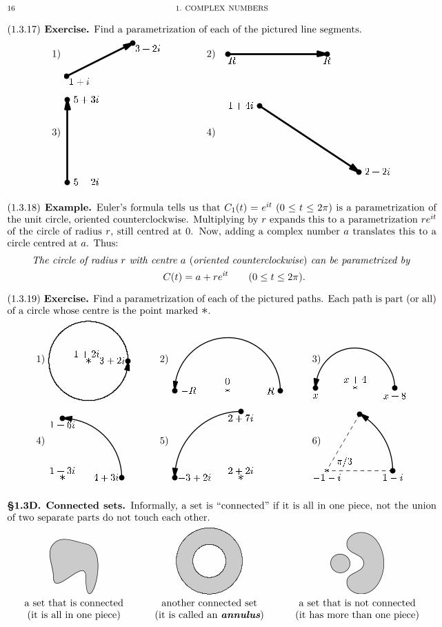
(1.3.17) Exercise. Find a parametrization of each of the pictured line segments.
1)
1 + i
3 + 2i 2) −R R
3)
5− 2i
5 + 3i
4)
−1 + 4i
2 + 2i
(1.3.18) Example. Euler’s formula tells us that C1(t) = eit (0 ≤ t ≤ 2π) is a parametrization ofthe unit circle, oriented counterclockwise. Multiplying by r expands this to a parametrization reit
of the circle of radius r, still centred at 0. Now, adding a complex number a translates this to acircle centred at a. Thus:
The circle of radius r with centre a (oriented counterclockwise) can be parametrized byC(t) = a + reit (0 ≤ t ≤ 2π).
(1.3.19) Exercise. Find a parametrization of each of the pictured paths. Each path is part (or all)of a circle whose centre is the point marked ∗.
1) 3 + 2i∗1 + 2i 2)
R−R ∗03)
x+ 8x∗x+ 4
4)
4 + 3i
1 + 6i
∗1 + 3i
5)
−3 + 2i
2 + 7i
∗2 + 2i
6)
1− i∗−1− i
π/3
§1.3D. Connected sets. Informally, a set is “connected” if it is all in one piece, not the unionof two separate parts do not touch each other.
a set that is connected another connected set a set that is not connected(it is all in one piece) (it is called an annulus) (it has more than one piece)

1.3. BASIC CONCEPTS OF TOPOLOGY 17
Another way of saying this is that if a set is connected, then it is possible to travel between anytwo points of the set, without ever leaving the set. Here is a formalization of that idea:
(1.3.20) Definition.(1) An open subset R of C is connected if, for all z1, z2 ∈ R, there is a path in R from z1 to z2,
i.e., a path C : [a, b] → C, such that C(a) = z1 and C(b) = z2, and C(t) ∈ R for all t.(2) A region is a nonempty, connected, open subset of C.
(1.3.21) Other terminology.(1) Some textbooks use the term “domain” for what we have called a region.(2) Officially, sets that satisfy the above definition should be called “path connected,” rather than
merely “connected.” (Mathematicians say that a set is “connected” if it is not the union oftwo nonempty, disjoint, open subsets.) However, it can be shown that the two notions areequivalent to each other when restricted to open subsets of C, so, in the setting where we areusing this terminology, it does no harm to say “connected,” rather than the slightly longerphrase “path connected.”
(1.3.22) Exercise. Show:(1) The union of two open sets is open.(2) The intersection of two open sets is open.(3) The union of two regions does not have to be a region.(4) The intersection of two regions does not have to be a region (even if it is not empty).(5) If two regions have nonempty intersection, then their union is a region.
By definition, any two points of a region are connected by a path. A priori, the path might bevery wiggly or have other problems, but the following helpful lemma (which we will assume withoutproof) shows that a very simple type of path can always be found. In light of this, many textbooksdefine a region to be a nonempty, open set in which every pair of points can be joined by a pathof the simple form described in the lemma, because that is probably the most straightforward wayto make this course completely rigorous.
(1.3.23) Lemma. Any two points of a region R can be joined by a path in R that consists of achain of finitely many horizontal and vertical line segments, joined end-to-end.
(1.3.24) Warning. The conclusion of the lemma often fails for connected sets that are not open.For example, the line y = x is connected, but it does not contain any horizontal or vertical linesegments at all, so it is impossible to move from a point to any other point by only moving eitherhorizontally or vertically.
(1.3.25) Examples.(1) Every open disk Dr(a) is connected. Indeed, any two points can be joined by a chain of (at
most) 2 horizontal or vertical line segments.

18 1. COMPLEX NUMBERS
(2) Every deleted neighbourhood Dr(a)× is connected. Indeed, any two points can be joined bya chain of (at most) 3 horizontal or vertical line segments.
(1.3.26) Exercise. (a) Sketch a picture of each set, then (b) determine whether the set is open ornot, and (c) whether it is connected or not. (You do not need to justify your answers.)
(1) C(2) C ∖ {0}(3) R(4) R ∖ {0}
(5) Im z > 3(6) Im z = 3(7) |Re z| > 3(8) |Re z| < 3
(9) |z| < 6(10) |z| > 6(11) {z : |z−5+2i| ≤ 4}(12) {z : |z−5+2i| > 4}
(13) D1(0) ∪ D1(1)(14) D1(0) ∪ D1(3)(15) C1(0) ∪ C2(0)(16)
{z : |z−5| ≥ |z|
}
1.4. Functions as mappingsHigh-school algebra typically deals with a function y = f(x), where x and y are in R. However,
when graphing the function, we often think of x and y as being in two different copies of R, namely,the x-axis and the y-axis. In Complex Analysis, we have a function w = f(z), whose domain andrange are in C. Analogous to what was done for x and y in high school, it can be helpful to thinkof z and w as being in two different copies of C, called the z-plane and the w-plane. The termcomplex mapping refers to viewing f as a function whose domain is in the z-plane, and whoserange is in the w-plane. We can illustrate the mapping w = f(z) by drawing a set X in the z-planeand its image f(X) in the w-plane.
(1.4.1) Examples.
(1) Consider the function f(z) = iz. This is a counterclockwise rotation of π/2 (or 90 degrees)about the origin. This can be illustrated by:
X1f(z) = iz
−→
f(X)
i
The picture on the left is a set X in the domain (or z-plane), and the picture on the right isits image f(X) in the w-plane.

1.4. FUNCTIONS AS MAPPINGS 19
(2) Now let f(z) = z2. Using the same set X for this function yields the following picture:
X1f(z) = z2
−→f(X)1
This picture was drawn by first finding the image of the two paths that form the boundaryof X: C1(t) = 1 + (1 + i)t (0 ≤ t < ∞) and its conjugate C2(t)1 + (1 − i)t (0 ≤ t < ∞).
For z = 1 + (1 + i)t = (1 + t) + ti, we have
z2 =((1+t)+ti
)2 =((1+t)2−t2
)+2t(1+t)i = (1+2t+t2−t2)+2t(1+t)i = (1+2t)+2t(1+t)i.
Thus, if we let x = Re z2 and y = Im z2, then x = 1 + 2t and y = 2t(1 + t). This implies2t = x − 1, so a bit of algebra shows that
y = (x − 1)(
1 +x − 1
2
)=
x2 − 12
.
This is the equation of a parabola. Similarly, the lower boundary f(C2(t)
)is on the parabola
y = −(x2 − 1)/2.(3) To illustrate the function f(z) = ez, it is helpful to look at the rectangular coordinate system
in the z-plane. This is based on vertical lines x = c and horizontal lines y = c.• If z = c + it, then ez = ec+it = ec · eit. This means that, as t varies, the absolute value
of z does not change, but the argument takes all possible values. Thus, ez covers all ofthe points in the circle of radius ec that is centred at the origin:
ez maps vertical lines to circles centred at the origin.• If z = t + ci, then ez = et+ci = et · eic. In this case, the argument c is constant, but the
absolute value takes on all possible positive values. Thus, as t varies, this covers all ofthe points in the ray from the origin that is at angle c from the positive real axis:
ez maps horizontal lines to rays from the origin.This is the picture, if we take vertical lines x = k (for k ∈ Z) and horizontal lines y = ℓπ/m(for ℓ ∈ Z), with, say m = 8:
0f(z) = ez
−→
This means that ez maps the rectangular coordinate system to the system of polar coordinates.

20 1. COMPLEX NUMBERS
(1.4.2) Exercises.(1) Find the image of each line under the function f(z) = z2:
(a) Re z = 1, (b) Im z = 1, (c) Re z = Im z, (d) Re z + Im z = 2.(2) Find the image of the first quadrant { z | Re z ≥ 0 and Im z ≥ 0 } under each of the following
functions:(a) f(z) = z2, (b) f(z) = z3, (c) f(z) = z, (d) f(z) = z + i.
(3) Find the image of the given set under the function f(z) = ez.(a) { z | 0 ≤ Re z ≤ 1 }. (b) { z | 0 ≤ Im z ≤ π/4 }.
1.5. Branch cutsYou know that every positive real number x has two different square roots. To make
√x
well-defined, we choose the square root that is ≥ 0; this is called the principal square root of x.A similar issue arises with defining the argument of z, because reiθ = rei(θ+2π). In this case,
mathematicians have agreed on the following definition:
(1.5.1) Definition. For z ∈ C \ {0}, the principal argument of z (denoted Arg z) is the angleθ ∈ (−π, π] that is an argument of z. (That is, such that we may write z = reiθ, for some r ≥ 0.)
(1.5.2) Note. The function Arg z is not continuous at points on the negative real axis, becauseArg z is close to
• π for points that are slightly above the axis, but• −π for points that are slightly below the axis.
The value of the function Arg z makes a big jump as it crosses the negative real axis, so it is notcontinuous there.
Therefore, if you want Arg z to be continuous, then you need to stay away from the negativereal axis, which is a ray from the origin. This ray is called the branch cut of Arg z, and Arg iscontinuous on complement of this branch cut. In other words, Log z is continuous in the regionC \ {x ∈ R | x ≤ 0 }:
0Arg z ≈ π
Arg z ≈ −πArg z ≈ 0
Arg z ≈ π/2
Arg z ≈ −π/2
If you are interested in the arguments of points that are on or near the negative real axis, thenyou could choose a different branch cut.
(1.5.3) Exercises.(1) Suppose we define Arg+ z to be the argument of z that is in the interval [0, 2π).What is the
branch cut of Arg+?(2) What is the branch cut of the function Arg∗ z that is defined to be the argument of z that is
in the interval (−π/2, 3π/2]? (The good thing about this branch is that it is continuous atall points of R, except 0, where it is not defined.)

1.5. BRANCH CUTS 21
A similar issue arises in many other cases. The general problem is that, instead of giving asingle value of f(z), some “functions” actually give a set of possible values. Such functions are saidto be “multi-valued” (as opposed to having only a single value).
(1.5.4) Definition. A multivalued function on a region R is a function f , such that f(z) is asubset of C for each z ∈ R.
(1.5.5) Example. Examples of multivalued functions include:(1) The argument of z: every complex number has infinitely many possible arguments.(2) z1/n: the number of nth roots of any nonzero complex number is n.
Given a multivalued function f , we would often like to choose a single value for each z (atleast, for each z in some region). This choice is called a “branch” of f . We will usually use thecorresponding upper-case letter F to represent a branch of a multivalued function f :
(1.5.6) Definition. Suppose f is a multivalued function on some region R, and R′ is a region thatis contained in R. We say that F : R′ → C is a branch of f if
(1) F (z) ∈ f(z) for all z ∈ R′, and(2) F is continuous on R′.
(1.5.7) Examples.(1) Arg z is a branch of the multi-valued function arg z on the region C \ {x | x ≤ 0 }.(2) The principal nth root of z is defined to be n
√z = |z|1/n ei(Arg z)/n. This is a branch of the
multivalued function z1/n. Its branch cut is the negative real axis (because it is defined fromArg z, which has a branch cut along the negative real axis).
(3) The principal logarithm of z is defined to be Log z = log |z| + (Arg z)i. This is a branchof the multivalued function log z. As in the previous examples, its branch cut is the negativereal axis.
(1.5.8) Exercise.(1) Calculate Log i and Log(−e2i).(2) Verify that:
(a)(
n√
z)n = z, so n
√z is indeed a branch of z1/n.
(b) eLog z = z, so Log z is indeed a branch of log z.(c) n
√z = e(Log z)/n for all z ∈ C and n ∈ Z+.
(3) Find z ∈ C, such that 3√
z and Log z exist, but(a) 3
√z3 = z and
(b) Log ez = z.(4) Find z1, z2 ∈ C, such that Log(z1z2) = Log z1 + Log z2 (and Log z1, Log z2, and Log(z1z2) all
exist).
(1.5.9) Remark. The formula in Exercise 1.5.8(2c) could be used as the definition of the principalbranch n
√z of z1/n. Generalizing this, the principal branch of the function zc is given by ec Log z,
for any c ∈ C. (We also say that the principal value of zc is ec Log z.) As you probably expect,the branch cut of this principal branch is the negative real axis.
(1.5.10) Exercise. Calculate the principal value of each exponential:(1) 23+2i, (2) ii, (3) (1 + i)1−i.


CHAPTER 2
Limits, Continuity, and Derivatives
2.1. LimitsThe difference between calculus courses and precalculus courses is that calculus includes limits,
which are the foundation of the key concepts of calculus: derivatives, integrals, and the notion of“continuous.”(2.1.1) Recall. From your calculus courses, you know that limx→a f(x) = L means f(x) is closeto L whenever x is close to a (but not equal to a). In words, we say that the limit of f(x) is L, asx approaches a.
The definition of “limit” is exactly the same for complex numbers, except that we use z in theplace of x.(2.1.2) Recall. Knowing that limz→a f(z) = L does not imply that f(a) = L. In fact, f(a) mightnot even exist. For example, if f(z) = z/z, then limz→0 f(z) = 1, but f(0) = 0/0 does not exist.It is precisely for the continuous functions that we have limz→a f(z) = f(a) (see 2.2.1).(2.1.3) Remark. The above “definition” is informal, not rigorous, but it is sufficient for the timebeing. We will see the official definition in §2.6; it uses ϵ and δ as in an ordinary calculus course.
We have the same limit laws as in ordinary calculus:(2.1.4) Limit laws. Assume limz→a f(z) and limz→a g(z) exist.
(1) The limit of a sum is the sum of the limits:if f(z) is close to A and g(z) is close to B, then f(z) + g(z) is close to A + B.
I.e.,limz→a
(f(z) + g(z)
)= lim
z→af(z) + lim
z→ag(z).
(2) The limit of a product is the product of the limits:if f(z) is close to A and g(z) is close to B, then f(z) g(z) is close to AB.
I.e.,limz→a
(f(z) g(z)
)=(limz→a
f(z))·(limz→a
g(z)).
(3) The limit of a quotient is the quotient of the limits if the denominator is not 0:if f(z) is close to A and g(z) is close to B (and B = 0), then f(z)/g(z) is close to A/B.
I.e.,
limz→a
f(z)g(z)
=limz→a
f(z)
limz→a
g(z)if lim
z→ag(z) = 0.
(4) If z is close to a, then z is close to a:limz→a
z = a.
(5) If z is close to a (or even if it isn’t), then any constant is close to itself:limz→a
c = c if c is a constant.
As you probably know, combining the limit laws with high-school algebra makes it possible tocalculate many limits.
23

24 2. LIMITS, CONTINUITY, AND DERIVATIVES
(2.1.5) Example. Calculate limz→2
z2 − 4z2 − z − 2
.
Solution. We have
limz→2
z2 − 43z2 − 5z − 2
= limz→2
(z + 2)(z − 2)(3z + 1)(z − 2)
= limz→2
z + 23z + 1
=limz→2
z + limz→2
2(limz→2
3)(
limz→2
z)
+ limz→2
1=
2 + 23 · 2 + 1
=47. □
(2.1.6) Exercise. Use the Limit Laws to calculate the following limits:
(1) limz→0
2z3 − 5z
z2 + 3iz, (2) lim
w→2
w2 − 2w
(w − 2)(w − 4i), (3) lim
z→i
z3 + i
z2 + 1,
It is a basic fact of ordinary calculus that if f is a function defined on R, and limx→a f exists,then this limit must be equal to the limits as x approaches a from each of the two sides (left andright):
limx→a
f = limx→a−
f = limx→a+
f.
For functions on C, the variable z can approach a from many directions, or even spiral toward itstarget, so that it does not approach from any particular direction:
If limz→a f(z) exists, then f(z) must tend to the same number L, no matter which path z takes toapproach a.
(2.1.7) Example. Calculate limz→0
z
z.
Solution. We havelimz→0
z
z= lim
x,y→0
x + iy
x + iy= lim
x,y→0
x − iy
x + iy.
Note that:• If z approaches 0 horizontally (i.e., along the x-axis, or “real axis”), then y = 0, so z/z
simplifies to x/x = 1.• If z approaches 0 vertically (i.e., along the y-axis, or “imaginary axis”), then x = 0, so z/z
simplifies to −y/y = −1.Thus, f(z) is close to 1 as z approaches 0 via one path (the x-axis, or “real axis”), but it is closeto a different number (namely −1) as z approaches via a different path (the y-axis or “imaginaryaxis”). So there is no single number that f(z) is close to when z approaches 0. This means thatthe limit does not exist. □
(2.1.8) Exercise. Show that limz→0
Re z
zdoes not exist.
In ordinary calculus, some limits tend to +∞, and others tend to −∞ (rather than approachingsome number L). However, in C, a point can go off to infinity in infinitely many different directions,and we do not distinguish between them:

2.2. CONTINUITY 25
(2.1.9) Definition. To say that limz→a f(z) = ∞ means |f(z)| is very large (as large as you like)whenever z is close to a (but not equal to a). In words, we say that the limit of f(z) is infinity, asz approaches a.
(2.1.10) Fact. If limz→a f(z) = L, for some L = 0, and limz→a g(z) = 0, then limz→a
f(z)g(z)
= ∞.
(2.1.11) Example. We have limz→a
1z(z − 1)
= ∞ when a = 0 or a = 1. (This is the function f(z)
that was graphed in Example 1.2.5.)
2.2. ContinuityThe following notion is the same as in an ordinary calculus course (except that the domain of
a function in a calculus textbook is a subset of R, rather than C, and x has been changed to z):
(2.2.1) Definition. Let f be a function whose domain is some subset of C, and let a ∈ C. We saythat f is continuous at a if lim
z→af(z) = f(a).
(2.2.2) Example. Use the Limit Laws to show that the function f(z) = 2z2 + 3iz is continuous atevery point.
Solution. For every a ∈ C, we havelimz→a
f(z) = limz→a
(2z2 + 3iz) = 2(
limz→a
z)2
+ 3i limz→a
z = 2(a)2 + 3i(a) = f(a). □
(2.2.3) Definition. For any a0, a1, . . . , an ∈ C, the function f(z) =∑n
k=0 akzk is called a
polynomial.
For example:• A typical polynomial is an expression something like 5 + 4z + 3z2 + 2z4. (Note that this
example has no z3-term: the coefficient of zk can be 0.)• The powers z, z2, z3 . . . are polynomials (and also z0, which is the constant function 1).•√
z = z1/2 and 1/z = z−1 are not polynomials: the exponents in a polynomial must beintegers (not fractions, such as 1/2) and are not allowed to be negative. In other words, theexponents must be in the set N of natural numbers.
• A power series, such as 1 + z + z2 + z3 + · · · , is not a polynomial, unless all but finitely manyof the terms are zero.
(2.2.4) Example. Every polynomial function is continuous at every point of C.
Proof. Let f(z) =∑n
k=0 akzk be any polynomial, and let a ∈ C. Note that, for each k, we have
limz→a
zk = limz→a
(z · z · · · z︸ ︷︷ ︸k factors
) (definition of kth power)
=(
limz→a
z)·(
limz→a
z)· · ·(
limz→a
z)
︸ ︷︷ ︸k factors
(the limit of a product isthe product of the limits
)
=(
limz→a
z)k (definition of kth power)
= ak.

26 2. LIMITS, CONTINUITY, AND DERIVATIVES
Therefore
limz→a
f(z) = limz→a
n∑k=0
akzk (definition of f(z))
=n∑
k=0
limz→a
(akzk)
(the limit of a sum is the sum of the limits
or “you can pull a summation out of a limit”
)
=n∑
k=0
ak limz→a
zk
the limit of a product is the product of the limits(and the limit of a constant is that constant)
or “you can pull a constant multiple out of a limit”
=
n∑k=0
ak · ak (established at the start of the proof)
= f(a) (definition of f(z)).So f is continuous at a. □
(2.2.5) Exercise. Prove by induction that limz→a zk = ak for all k ∈ N.(This justifies a crucial step that was not rigorous in the above proof. The issue is that 2.1.4(2)
only applies to a product that has 2 factors, not a product with k factors.)
The limit laws show that certain combinations of continuous functions are continuous:
(2.2.6) Exercise. Let a, c ∈ C, and assume f and g are continuous at a. Show that:f + g is continuous at a. (The sum of continuous functions is continuous.)(1)f − g is continuous at a. (The difference of continuous functions is continuous.)(2)cf is continuous at a. (A constant multiple of a continuous function is continuous.)(3)fg is continuous at a. (The product of continuous functions is continuous.)(4)f/g is continuous at a
if g(a) = 0.
(The quotient of continuous functions is continuous
if the denominator is not zero.
)(5)
(2.2.6) Definition. Recall that a rational function is a quotient P (z)/Q(z) of two polynomials.Its domain is the set of points where the denominator is not zero.
For example, (z2 + 1)/(5z3 − 2z + 4) is a rational function.
(2.2.7) Corollary. Any rational function is continuous at every point in its domain.
(2.2.8) Remark. We will see in Exercise 2.3.24 that ez, sin z, and cos z are continuous at everypoint of C.
2.3. Derivatives§2.3A. Differentiation. The definition of derivative in this course is the same as in ordinarycalculus (except that it allows complex numbers):
(2.3.1) Definition. Let f be a function whose domain is some subset of C.• The derivative of f at z is:
d
dzf(z) = f ′(z) = lim
h→0
f(z + h) − f(z)h
= limw→z
f(w) − f(z)w − z
.
• f is differentiable at z if f ′(z) exists.
You probably remember from your first calculus class that the derivative of x2 is 2x. So youwould expect the derivative of z2 to be 2z. That is indeed correct:

2.3. DERIVATIVES 27
(2.3.2) Example. Show that ddz z2 = 2z.
Solution. Let f(z) = z2. Then
f ′(z) = limh→0
f(z + h) − f(z)h
(definition of derivative)
= limh→0
(z + h)2 − z2
h(definition of f)
= limh→0
(z2 + 2zh + h2) − z2
h
= limh→0
2zh + h2
h= lim
h→0(2z + h)
= 2z + limh→0
h (2z is a constant in this limit)
= 2z + 0= 2z. □
More generally, the derivative of zn is nzn−1, as you would expect. Many other well-knowndifferentiation rules also hold:
(2.3.3) Exercise (Differentiation Rules). Assume that f and g are differentiable. Show that:
(1) The derivative of a constant is zero: ddz c = 0 if c is a constant.
(2) The derivative of a constant multiple is that multiple of the derivative: ddz cf(z) = cf ′(z).
(or “You can pull a constant multiple out of a derivative.”)
(3) The derivative of a sum is the sum of the derivatives: ddz
(f(z) + g(z)
)= f ′(z) + g′(z).
(or “You can break up the derivative of a sum.”)
(4) Product Rule: ddz
(f(z) g(z)
)= f ′(z)g(z) + f(z)g′(z).
(Important: “The derivative of a product is not the product of the derivatives.”)
(5) Quotient Rule: d
dz
f(z)g(z)
=f ′(z) g(z) + f(z) g′(z)
g(z)2if g(z) = 0.
(Important: “The derivative of a quotient is not the quotient of the derivatives.”)
(6) Chain Rule: ddzf(g(z)
)= f ′(g(z)
)g′(z).
(“If you treat a quantity as the variable of differentiation,then you need to multiply by the derivative of that quantity.”)
(7) Power Rule: ddz zn = n zn−1 if n is an integer (and z = 0, if n < 0).
[Hint. For the Product Rule (and any others where it is helpful), you may use the fact that differentiablefunctions are continuous (see Exercise 2.3.11).]
(2.3.4) Remark. The Power Rule (7) also applies when n is not an integer if branches of themultivalued functions zn and zn−1 are chosen correctly (see Exercise 2.3.28(2)).
(2.3.5) Example. Calculate the derivative of f(z) =z2 − 4
3z2 − 5z − 2.

28 2. LIMITS, CONTINUITY, AND DERIVATIVES
Solution. We have
f ′(z) =d
dz
(z2 − 4
3z2 − 5z − 2
)=
(z2 − 4)′ (3z2 − 5z − 2) − (3z2 − 5z − 2)′ (z2 − 4)(3z2 − 5z − 2)2
(Quotient Rule)
=(2z − 0)(3z2 − 5z − 2) −
(3(2z) − 5 − 0
)(z2 − 4)
(3z2 − 5z − 2)2
= · · · (high-school algebra omitted)
=−5z2 + 20z − 20(3z2 − 5z − 2)2
. □
(2.3.6) Example. Calculate the derivative of f(z) = (2z + 1)100.
Solution. We havef ′(z) =
d
dz(2z + 1)100 = 100(2z + 1)99 · (2z + 1)′ (Chain Rule)
= 100(2z + 1)99 · 2 = 200(2z + 1)99. □
(2.3.7) Example. Suppose the function g is the inverse of the function f on some region R, sof(g(z)
)= z for all z ∈ R. Find g′(z) for z ∈ R.
Solution. We have1 =
d
dzz =
d
dzf(g(z)
)= f ′(g(z)
)g′(z) (Chain Rule).
Thereforeg′(z) =
1f ′(g(z)
) . □
(2.3.8) Example.(1) g(z) =
√z is an inverse of f(z) = z2, so (since f ′(z) = 2z) we have
d
dz
√z =
1f ′(g(z)
) =1
2g(z)=
12√
z.
Note that this is a special case of the well-known formula ddz zr = rzr−1.
(2) We will see that ddz ez = ez. If Log∗ z is any branch of log z, then it is an inverse of ez, so we
can conclude thatd
dzLog∗ z =
1eLog∗ z
=1z.
(2.3.9) Exercise. Calculate the derivative of each of the following functions.
(1) 5z7−(10+2i)z4+37z−6i, (2) (3z2 − 11)100, (3) z2 + i
z − 1.
In ordinary calculus, you learned that if the derivative of a function is 0 on some interval, thenthe function is constant in that interval. (This is an important consequence of the Mean ValueTheorem.) Here is the complex analogue:
(2.3.10) Exercise. Show that if f ′(z) = 0 for all z in some region, then f is constant on thatregion.

2.3. DERIVATIVES 29
[Hint. If C(t) is a differentiable curve, then ddtf(C(t)
)= f ′(C(t)
)· C ′(t) = 0 (why?). Any horizontal or
vertical line segment is a differentiable curve.]
Not all functions have a derivative. In particular, a function cannot be differentiable unless itis continuous:
(2.3.11) Exercise. Show that if f is differentiable at a, then f is continuous at a.[Hint. Show limz→a
(f(z) − f(a)
)= 0.]
(2.3.12) Warning. The converse is not true: there are many examples of continuous functions thatare not differentiable.
Here is one:
(2.3.13) Exercise. For all a ∈ C, show that f(z) = z is not differentiable at a.[Hint. Write z = x + yi. We will see another solution in Example 2.4.6.]
(2.3.14) Exercise. Prove a special case of L’Hôpital’s Rule: If f and g are differentiable at a,and f(a) = g(a) = 0, but g′(a) = 0, then
limz→a
f(z)g(z)
= limz→a
f ′(z)g′(z)
.
[Hint. Divide the numerator and denominator of the first limit by z − a.]
§2.3B. Holomorphic functions and poles.
(2.3.15) Definition.(1) f is holomorphic in a region R if it is differentiable at all points of R.(2) f is holomorphic at a point a if f is holomorphic in some neighbourhood of a. (This means
that f is differentiable not only at a, but also at all points that are close to a.)(3) If f is holomorphic on the entire complex plane C, then we say that f is entire.(4) We say that the point a of C is a pole of a function f if limz→a |f(z)| = ∞, but f is
holomorphic in some deleted neighbourhood of a.
(2.3.16) Exercise. Let f(z) = P (z)/Q(z) be a rational function (see Definition 2.2.6).(1) Show that f is holomorphic on its domain (i.e., on { z | Q(z) = 0 }).(2) Show that if Q(a) = 0 and P (a) = 0, then a is a pole of f .
(2.3.17) Example. f(z) =z2 − 3z + 2
z2 + 1is a rational
function. Its poles are at i and −i, because the roots ofz2 + 1 are ±i (and neither of these is a root of z2 − 3x + 2).The poles are obvious in the computer-generated graph of|f(z)| at right.
(2.3.18) Remark. Holomorphic functions preserve angles (at points where the derivative is not 0).This means that if C1 and C2 are two differentiable curves in C that intersect at a point a, and θ isthe angle between the curves at this point, then θ is also the angle between the curves f(C1) andf(C2) at the point f(a).
For example, it is obvious that horizontal lines are perpendicular to vertical lines. Since ez isentire, this implies that the image of any horizontal line under ez is perpendicular to the image ofany vertical line. Indeed, we know from Example 1.4.1(3) that the image of a horizontal line is aray from the origin, whereas the image of a vertical line is a circle centred at the origin, and theseare perpendicular to each other (see the picture in Example 1.4.1(3)).

30 2. LIMITS, CONTINUITY, AND DERIVATIVES
(2.3.19) Exercise. Prove the statement in Remark 2.3.18.[Hint. Assume, without loss of generality, that C1(0) = C2(0) = a. The angle between C1 and C2 is thesame as the angle between the tangent vectors v1 = C ′
1(0) and v2 = C ′2(0). If w = f ′(a), then the tangent
vectors of f(C1) and f(C2) are w v1 and wv2 (by the Chain Rule). Now apply Exercise 1.1.39(7).]
§2.3C. Derivative of ez and trigonometric functions. The students in an ordinary calculusclass learn that the derivative of ex is ex, so you would expect that the derivative of ez is ez. Thisis indeed true:
(2.3.20) Proposition. ddz ez = ez.
Proof. Let’s assume that the derivative of a power series can be calculated by differentiatingit term-by-term (as if it were a polynomial). (This will be justified in Theorem 4.3.2, but adifferent calculation of (ez)′ that does not require this fact about power series can be found inExercise 2.4.7(6).) Then, since
ez =∞∑
k=0
zk
k!= 1 + z +
z2
2+
z3
3!+
z4
4!+ · · · ,
we have
(ez)′ = 1′ + z′ +(z2)′
2+
(z3)′
3!+
(z4)′
4!+ · · ·
= 0 + 1 +2z
2+
3z2
3!+
4z3
4!+ · · ·
= 1 + z +z2
2!+
z3
3!+ · · ·
= ez. □
The same method can be used to calculate the derivatives of sin z and cos z:
(2.3.21) Exercises. Use term-by-term differentiation of power series to show that:(1) d
dz sin z = cos z and(2) d
dz cos z = − sin z.
An alternate approach to calculating sin′ z and cos′ z is to use the fact that sin z and cos z cancalculated from ez. (This approach is employed by textbooks that use these formulas to define sin zand cos z.)
(2.3.22) Example. We have sin z =eiz − e−iz
2i(see Note 1.1.27), so
sin′ z =(
eiz − e−iz
2i
)′
=(eiz)′ − (e−iz)′
2i
=eiz · i − e−iz · (−i)
2i(Chain Rule)
=eiz + e−iz
2= cos z (Note 1.1.27).
(2.3.23) Exercise. Use the method of Example 2.3.22 to obtain the derivative of cos z from thederivative of ez.

2.4. CAUCHY-RIEMANN EQUATIONS 31
(2.3.24) Exercise. Show that ez, sin z, and cos z are continuous at every point of C.
By using the derivatives of sin z and cos z, you can find the derivatives of all of the other trigfunctions.
(2.3.25) Example. Find the derivative of tan z.
Solution. We have tan z =sin z
cos z, so
(tan z)′ =(
sin z
cos z
)′=
(sin z)′ cos z − (sin z)(cos z)′
(cos z)2(Quotient Rule)
=(cos z) cos z − (sin z)(− sin z)
(cos z)2
=cos2 z + sin2 z
(cos z)2
=1
(cos z)2
=(
1cos z
)2
= sec2 z.
□
(2.3.26) Exercises. Show that:(1) d
dz sec z = sec z tan z.(2) d
dz cot z = − csc2 z.(3) d
dz csc z = − csc z cot z.[Hint. Recall that cot z = 1/tan z, sec z = 1/cos z, and csc z = 1/sin z.]
(2.3.27) Exercise. In addition to the usual trig functions (sine, cosine, etc.), you may haveencountered the hyperbolic trig functions in your previous calculus classes. Hyperbolic sine andhyperbolic cosine are defined by:
sinh z =ez − e−z
2and cosh z =
ez + e−z
2.
Calculate the derivative of (1) sinh z and (2) cosh z. (Remark. sinh is usually pronounced “sinsh.”)
(2.3.28) Exercises.(1) Show that d
dz log z = 1/z.[Hint. Implicit differentiation: differentiate both sides of the equation elog z = z, and solve for log′ z.]
(2) Show that if we take the principal branches of zc and zc−1, then ddz zc = c zc−1, for every
c ∈ C. [Hint. The principal branch of zc is ec Log z (see Remark 1.5.9).]
2.4. Cauchy-Riemann equations
Suppose f is differentiable at a, so limz→a
f(z) − f(a)z − a
exists. We must get the same limit fromall directions. In particular, if we write a = b + ci, then letting z = x + ci (with x → b) must givethe same limit as letting z = b + yi (with y → c):
limx→b
f(x + ci) − f(b + ci)(x + ci) − (b + ci)
= limy→c
f(b + yi) − f(b + ci)(b + yi) − (b + ci)
.
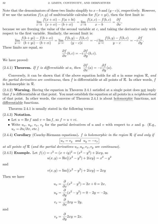
32 2. LIMITS, CONTINUITY, AND DERIVATIVES
Note that the denominators of these two limits simplify to x−b and (y−c)i, respectively. However,if we use the notation f(x, y) of multivariable calculus for f(x + yi), then the first limit is:
limx→b
f(x + ci) − f(a + bi)(x + ci) − (b + ci)
= limx→b
f(x, c) − f(b, c)x − b
=∂f
∂x,
because we are freezing the value of the second variable at c, and taking the derivative only withrespect to the first variable. Similarly, the second limit is:
limy→c
f(b + yi) − f(b + ci)(b + yi) − (b + ci)
= limy→c
f(b, y) − f(b, c)(y − c)i
= −i limy→c
f(b, y) − f(b, c)y − c
= −i∂f
∂y.
These limits are equal, so∂f
∂x(b, c) = −i
∂f
∂y(b, c).
We have proved:
(2.4.1) Theorem. If f is differentiable at a, then ∂f
∂x(a) = −i
∂f
∂y(a).
Conversely, it can be shown that if the above equation holds for all a in some region R, andthe partial derivatives are continuous, then f is differentiable at all points of R. In other words, fis holomorphic in R.(2.4.2) Warning. Having the equation in Theorem 2.4.1 satisfied at a single point does not implythat f is differentiable at that point. You must establish the equation at all points in a neighbourhoodof that point. In other words, the converse of Theorem 2.4.1 is about holomorphic functions, notdifferentiable functions.
Theorem 2.4.1 is usually stated in the following terms:(2.4.3) Notation.
• Let u = Re f and v = Im f , so f = u + vi.• Write ux, uy, vx, vy for the partial derivatives of u and v with respect to x and y. (E.g.,
ux = ∂u/∂x, etc.)(2.4.4) Corollary (Cauchy-Riemann equations). f is holomorphic in the region R if and only if
ux = vy and uy = −vx
at all points of R (and the partial derivatives ux, uy, vx, vy are continuous).(2.4.5) Example. Let f(z) = z2 = (x + iy)2 = (x2 − y2) + 2ixy, so
u(x, y) = Re((x2 − y2) + 2ixy
)= x2 − y2
andv(x, y) = Im
((x2 − y2) + 2ixy
)= 2xy
Then we have
ux =∂
∂x(x2 − y2) = 2x + 0 = 2x,
uy =∂
∂y(x2 − y2) = 0 − 2y = −2y,
vx =∂
∂x2xy = 2y,
and
vy =∂
∂y2xy = 2x.

2.4. CAUCHY-RIEMANN EQUATIONS 33
By comparing these results, we see thatux = 2x = vy and uy = −2y = −vx.
This means that the Cauchy-Riemann equations are satisfied everywhere, which agrees with thefact that f(z) = z2 is differentiable at all points. I.e., z2 is entire.
(2.4.6) Example. Let f(z) = z = x + iy = x − iy, sou(x, y) = Re(x − iy) = x
and
v(x, y) = Im(x − iy) = −y.
Then
ux =∂
∂xx = 1,
uy =∂
∂yx = 0,
vx =∂
∂x− y = 0,
and
vy =∂
∂y(−y) = −1.
Since ux = 1 but vy = −1, we see that ux = vy, so (at every point) the Cauchy-Riemann equationux = vy is not satisfied (although the other one is). This agrees with the fact that f(z) = z is notdifferentiable (see Exercise 2.3.13).
(2.4.7) Exercises.(1) Show that the function x3 − 3xy2 + (3x2y − y3)i satisfies the Cauchy-Riemann equations at
all points (so it is entire).(2) Find all points at which the function f(z) = |z|2 satisfies the Cauchy-Riemann equations. At
what points is this function holomorphic?(3) Find all points at which the function x2−y+(x+y2)i satisfies the Cauchy-Riemann equations.(4) Assume that (ax2 + by2 + cx)+(4xy +3y)i is holomorphic in some region. Find the constants
a, b, and c.(5) Show that if f is differentiable, then
f ′(z) = ux + vxi.
[Hint. f ′(z) is defined by a certain limit. Since this limit exists, it must be equal to the limit as h
approaches 0 along the real axis.](6) Assume that ex+iy = ex(cos y + i sin y) (but do not assume that ez is equal to its Taylor
Series). Use the Cauchy-Riemann equations (and (5)) to show that (ez)′ = ez. (In textbooksthat define ez via this formula for ex+iy, instead of by using the Taylor series, this is themethod that is used to calculate the derivative of ez.)
(7) Suppose f is holomorphic on the region R, and f(z) is real for all z ∈ R. Show that f isconstant.
(2.4.8) Remark. It can be shown that if f is holomorphic on the region R, and f is not constant,then f(R) is an open set. Since R does not contain any nonempty open subsets of C, this factimplies Exercise 2.4.7(7).

34 2. LIMITS, CONTINUITY, AND DERIVATIVES
2.5. Harmonic functionsHere is an important consequence of the Cauchy-Riemann Equations: if f = u + vi is
holomorphic, then
uxx + uyy =∂
∂xux +
∂
∂yuy (definition of uxx and uyy)
=∂
∂xvy −
∂
∂yvx
(Cauchy-Riemann Equations:
ux = vy and uy = −vx
)= vxy − vyx (where vxy =
∂
∂x
∂
∂yv and vyx =
∂
∂y
∂
∂xv)
= 0 (a theorem of multivariable calculus says that vxy = vyx).In the following terminology, this means that the real part of every holomorphic function is“harmonic”:(2.5.1) Definition. Let u be a real-valued function on a region R. We say that u is harmonicon R if uxx + uyy = 0 at all points of R.
Let us state this important fact as an official result:(2.5.2) Proposition. The real part of every holomorphic function is harmonic.(2.5.3) Exercise. Use the Cauchy-Riemann equations to show that the imaginary part of everyholomorphic function is harmonic.(2.5.4) Example. z2 is holomorphic, and
z2 = (x + iy)2 = (x2 − y2) + 2ixy,
so x2 − y2 and 2xy are harmonic.This can also be verified by direct calculation: if u(x, y) = x2 − y2 and v(x, y) = 2xy, then
uxx + uyy = (x2 − y2)xx + (x2 − y2)yy
=∂
∂x(x2 − y2)x +
∂
∂y(x2 − y2)y
=∂
∂x(2x − 0) +
∂
∂y(0 − 2y)
=∂
∂x(2x) − ∂
∂y(2y)
= 2 − 2= 0
andvxx + vyy = (2xy)xx + (2xy)yy
=∂
∂x(2xy)x +
∂
∂y(2xy)y
=∂
∂x(2y) +
∂
∂y(2x)
= 0 + 0= 0,
so u and v are harmonic.(2.5.5) Example. Let
u(x, y) = x3 + ax2 + by2 + cxy2 + dx.

2.5. HARMONIC FUNCTIONS 35
What choices of a, b, c, and d make u harmonic (on all of R2)?
Solution. We haveuxx =
∂
∂x
∂
∂x(x3 + ax2 + by2 + cxy2 + dx)
=∂
∂x(3x2 + a(2x) + 0 + cy2 + d)
=∂
∂x(3x2 + 2ax + cy2 + d)
= 3(2x) + 2a + 0 + 0= 6x + 2a
and
uyy =∂
∂y
∂
∂y(x3 + ax2 + by2 + cxy2 + dx)
=∂
∂y(0 + 0 + b(2y) + cx(2y) + 0)
=∂
∂y(2by + 2cxy)
= 2b + 2cx.
Thereforeuxx + uyy = 0 ⇐⇒ (6x + 2a) + (2b + 2cx) = 0 ⇐⇒ (6 + 2c)x + 2(a + b) = 0.
Saying that u is harmonic means that this function is 0 for all values of x (and y), sou is harmonic ⇐⇒ 6 + 2c = 0 and 2(a + b) = 0.
The equations on the right-hand side mean that c = −3 and b = −a (and there is no restrictionon d). Thus, c must be −3, but we can choose any values for a and d, and let b = −a.
In other words,u(x, y) = x3 + ax2 − ay2 − 3xy2 + dx is harmonic
for every choice of a and d. □
(2.5.6) Exercises.(1) Verify that each function is harmonic.
(a) x2 − y2
(b) 2xy
(c) 6x2y − 2y3
(d) x4+4x3y−6x2y2−4xy3+y4
(e) ex cos y
(f) log(x2 + y2)(2) Show that u(x, y) = sin x + sin y is not harmonic.(3) Suppose c is a real number. Show that if u is a harmonic function, then c u is also harmonic.(4) Show that if u and v are harmonic functions, then u + v is also a harmonic function.
Proposition 2.5.2 has a converse:
(2.5.7) Theorem. If u is a harmonic function on C, then u is the real part of a holomorphicfunction on C.
We postpone the proof of this theorem to Corollary 3.4.13 in §3.4, because it relies on someadditional theory that we have not seen yet. (The proof will establish a more general version thatallows C to be replaced with any region that is “simply connected” (see Definition 3.2.6).) For now,we will just do some examples, after introducing a bit of terminology.
(2.5.8) Definition. Let u and v be real-valued functions on a region R. If u + iv is holomorphicon R, then we say that v is a harmonic conjugate of u.
36 2. LIMITS, CONTINUITY, AND DERIVATIVES
In this terminology, Theorem 2.5.7 says that every harmonic function (that is defined on allof C) has a harmonic conjugate. The following example illustrates a general method that can beused to find it.
(2.5.9) Example. Find a harmonic conjugate of u(x, y) = 2x + 2xy − x3 + 3xy2.
Solution. We wish to find v, such that u + iv satisfies the Cauchy-Riemann equations:vy = ux = (2x + 2xy − x3 + 3xy2)x = 2 + 2y − 3x2 + 3y2
andvx = −uy = −(2x + 2xy − x3 + 3xy2)y = −(0 + 2x − 0 + 6xy) = −2x − 6xy.
Integrating the first equation with respect to y tells us
v =∫
(2 + 2y − 3x2 + 3y2) dy = 2y + y2 − 3x2y + y3 + C1(x).
It is important to note that the “constant of integration” can have x in it, since the integral iswith respect to y, and x is a constant when y is the only variable; thus, we write C1(x), instead ofonly C1. Similarly, integrating the second equation with respect to x tells us
v =∫
(−2x − 6xy) dx = −x2 − 3x2y + C2(y).
(This time, the constant of integration is a function of y, since y is a constant when x is the onlyvariable.)
Matching up these two expressions for v, we see that we may takeC1(x) = −x2 and C2(y) = 2y + y2 + y3.
Therefore,v = 2y + y2 − 3x2y + y3 − x2
is a harmonic conjugate of u. □
(2.5.10) Remark (alternate solution). Sometimes, it may not be obvious how to match up the twoexpressions for v. (For example, perhaps it relies on an obscure trig identity.) So here is a slightlymodified method that avoids this step.
We wish to find v, such that u + iv satisfies the Cauchy-Riemann equations:vy = ux = (2x + 2xy − x3 + 3xy2)x = 2 + 2y − 3x2 + 3y2
andvx = −uy = −(2x + 2xy − x3 + 3xy2)y = −(0 + 2x − 0 + 6xy) = −2x − 6xy.
Integrating the first equation with respect to y tells us
v =∫
(2 + 2y − 3x2 + 3y2) dy = 2y + y2 − 3x2y + y3 + C(x).
Differentiating this formula with respect to x yields
vx =∂
∂x(2y + y2 − 3x2y + y3 + C(x)) = 0 + 0 − 6xy + 0 + C ′(x) = −6xy + C ′(x).
By equating this to our previous formula for vx, we see that−2x − 6xy = vx = −6xy + C ′(x),
so C ′(x) = −2x. Integrating both sides with respect to x tells us
C(x) =∫
−2x = −x2 + C1.
Choosing C1 = 0, we obtain the functionv = 2y + y2 − 3x2y + y3 + C(x) = 2y + y2 − 3x2y + y3 − x2.

2.6. THE OFFICIAL DEFINITION OF A LIMIT 37
We know from Exercise 2.5.6(2) that sin x+sin y is not harmonic. Therefore, this function doesnot have a harmonic conjugate. Let’s see what happens if we try to find one:
(2.5.11) Example. Use the above method to try to find a harmonic conjugate of sin x + sin y.
Solution. Let u(x, y) = sin x + sin y. We wish to find v, such that u + iv satisfies the Cauchy-Riemann equations:
vy = ux = (sin x + sin y)x = cos x + 0 = cos x
andvx = −uy = −(sin x + sin y)y = −(0 + cos y) = − cos y.
Integrating the first equation with respect to y tells us
v =∫
cos x dy = y cos x + C1(x).
Integrating the second equation with respect to x tells us
v =∫
(− cos y) dx = −x cos y + C2(y).
It is impossible to match these two expressions for v by choosing C1(x) and C2(y), so the harmonicconjugate does not exist. (The condition uxx + uyy = 0 is exactly what guarantees that it will bepossible to choose C1(x) and C2(y) appropriately.) □
(2.5.12) Exercise. Find a harmonic conjugate of the given function.(1) 5x + 7y
(2) 6x2y − 2y3
(3) x4 + 4x3y − 6x2y2 − 4xy3 + y4
(4) ex cos y
(5) ex (x cos y − y sin y)(6) 2 arctan(y/x) [Hint. arctan′(x) = 1/(x2 +1).](7) x3 + ax2 − ay2 − 3xy2 + bx,
where a and b are constants
(2.5.13) Exercise. Show that if v1 and v2 are harmonic conjugates of a function u on a region R,then there is a constant C, such that v1 = v2 + C.
2.6. The official definition of a limit(2.6.1) Recall. lim
z→z0
f(z) = L means f(z) is close to L whenever z is close to z0 (but not equalto z0).
More precisely, if we have an acceptable tolerance, which specifies how close f(z) needs to beto L (this bound is usually called ϵ), then there is a corresponding margin of error (which is usuallycalled δ), such that if z is within the margin of error of being equal to z0 (but is not equal to z0),then |f(z) − L| is guaranteed to be within the given tolerance.
Here is the official definition:
(2.6.2) Definition. Assume f is a function on some region R, and z0 ∈ C. To say thatlimz→z0 f(z) = L means: for every ϵ > 0, there exists δ > 0, such that, for all z ∈ C, if0 < |z − z0| < δ, then |f(z) − L| < ϵ.
The definition can also be phrased in the language of topology (§1.3):
(2.6.3) Exercise. Assume f is defined on some region R, and z0 ∈ C. Show that limz→z0 f(z) = Liff for every neighbourhood D of L, there is a deleted neighbourhood D′ of z0, such that f(z) ∈ Dfor all z ∈ D′.
(2.6.4) Example. Suppose f(z) = z2. Then f(2) = 4. Therefore, if z is close to 2, then f(z)should be close to 4.

38 2. LIMITS, CONTINUITY, AND DERIVATIVES
In particular, suppose we need to know that |f(z) − 4| < 0.1. (So ϵ = 0.1.) How close does zneed to be to 2? (I.e., what is the corresponding δ?)
(2.6.5) Scratchwork. Assume |z − 2| < δ. Want: |f(z) − 4|?< 0.1.
|f(z) − 4| = |z2 − 4|= |z − 2| · |z + 2|< δ · |(z − 2) + 4|≤ δ(|z − 2| + 4
)(Triangle Inequality)
≤ δ(δ + 4
)≤ δ · 5 (if δ < 1)?≤ 0.1.
Therefore, to make |f(z) − 4| < 0.1, we just need to make 5δ ≤ 0.1 (and δ ≤ 1). So we letδ = 0.1/5 = 0.02.
Solution. It suffices to require |z−2| to be less than 0.02. To verify this, note that if |z−2| < 0.02,then
|f(z) − 4| = |z2 − 4|= |z − 2| · |z + 2|< 0.02 · |(z − 2) + 4|≤ 0.02
(|z − 2| + 4
)(Triangle Inequality)
≤ 0.02(0.02 + 4
)< 0.02 · 5= 0.1. □
For any ϵ > 0, the same calculation shows that if δ = min(ϵ/5, 1), and |z − 2| < δ, then|z2 − 4| < ϵ. This means limz→2 z2 = 4.(2.6.6) Exercises.
(1) For all w ∈ C, prove directly from the definition of limit that limz→w z2 = w2.(2) For a, b, w ∈ C, prove directly from the definition of limit that limz→z0(az + b) = az0 + b.(3) Prove the Limit Laws (2.1.4).(4) Assume f is a continuous function on a region R. Show that { z ∈ R | f(z) = 0 } is open.(5) Assume f is a function on a region R, and a ∈ R. Show that f is continuous at a if and only
if: for every ϵ > 0, there exists δ > 0, such that|f(z) − f(a)| < ϵ for all z ∈ Dδ(a).
(Remark: The first two exercises show that the functions z2 and az + b are continuous on all of C.)And here is the official definition of limits that are infinite (cf. Definition 2.1.9):
(2.6.7) Definition. Assume f is defined on some region R, and z0 ∈ C. To say thatlimz→z0 f(z) = ∞ means: for every M ∈ R, there exists δ > 0, such that, for all z ∈ C, if0 < |z − z0| < δ, then |f(z)| > M .
Like Definition 2.6.2, this definition can also be phrased in the language of topology:(2.6.8) Exercise. Assume f is defined on some region R, and z0 ∈ C. Show that limz→z0 f(z) = ∞iff for every M ∈ R, there is a deleted neighbourhood D′ of z0, such that |f(z)| > M for all z ∈ D′.

2.6. THE OFFICIAL DEFINITION OF A LIMIT 39
(2.6.9) Exercise. Prove Fact 2.1.10.
Later in the semester, we will also be interested in limits as a real variable r gets very large:
(2.6.10) Definition. Assume f(r) is a function that is defined for all large real values of r. Tosay that limr→∞ f(r) = L means: for every ϵ > 0, there exists M > 0, such that, for all r ∈ R, ifr > M , then |f(r) − L| < ϵ.
(2.6.11) Exercise.
(1) Show that limr→∞
1r
= 0.
(2) Show that if |f(r)| ≤ g(r) for all r, and limr→∞ g(r) = 0, then limr→∞ f(r) = 0. (This isoften called the Squeeze Theorem or Sandwich Theorem.)


CHAPTER 3
Integration
3.1. Contour integrals
In ordinary calculus, the expression∫ ba f(x) dx denotes the integral of f from a to b, or, in other
words, the integral of f on the interval [a, b]. You might therefore expect that the integrals in thiscourse would be denoted
∫ ba f(z) dz. However, specifying the endpoints a and b of an integral in the
complex plane does not determine the route that should be taken to get from a to b, and (as we willsee) different routes sometimes result in different values of the integral. Therefore, an integral mustspecify the route (or, in technical terms, “path”) that is to be traversed when travelling from ato b. Thus, the notation for an integral is
∫C f(z) dz, where C is a path in C.
To calculate the integral∫C f(z) dz, make a change of variables (or “substitution”), letting
z = C(t) (so dz = C ′(t) dt):
(3.1.1) Definition. If f is a continuous function on a region R, and C : [a, b] → R is a path in R,then
∫C
f(z) dz =∫ b
af(C(t)
)C ′(t) dt.
We call this a contour integral. (Recall that the path C is also known as a “contour”(see Note 1.3.13).)
(3.1.2) Notation. We will often abbreviate∫C f(z) dz to
∫C f .
(3.1.3) Note. Since the expression in Definition 3.1.1 involves C ′(t), this definition requires thepath C to be differentiable. Actually, if we subdivide the interval [a, b] into subintervals [ti, ti+1](so a1 = t0 < t1 < t2 < · · · < tn = b), then the integral from a to b can be broken up into pieces:∫ b
af(C(t)
)C ′(t) dt =
∫ t1
t0
f(C(t)
)C ′(t) dt +
∫ t2
t1
f(C(t)
)C ′(t) dt + · · · +
∫ xn
tn−1
f(C(t)
)C ′(t) dt.
Therefore, it suffices for C to be piecewise differentiable, which means it consists of finitelymany differentiable curves C1, . . . , Cn that have been joined end-to-end. Thus, there can be finitelymany values of t at which C is not differentiable (e.g., C may have some corners or cusps).
Actually, there is a technical issue that we want the derivative C ′(t) to be continuous, not justto exist, and not to be zero.
(3.1.4) Definition. A curve whose derivative is continuous (and never 0) is said to be smooth.
(3.1.5) Assumption. Henceforth, all paths (or curves or contours) will always be assumed to bepiecewise smooth.
41

42 3. INTEGRATION
a smooth curve a piecewise smooth curve another piecewisesmooth curve
(3.1.6) Remark. Definition 3.1.1 will suffice for our purposes, but the official definition of∫C f uses
Riemann sums that are obtained by dividing the path C into small pieces, much like the definitionof∫ ba f(x) dx in an ordinary calculus class:
(1) Choose z0 = C(t0), z1 = C(t1), . . . , zn = C(tn) on C, with a = t0 < t1 < t2 < · · · < tn = b,
(2) for each k, choose z∗k = C(t∗k) for some t∗k ∈ [tk−1, tk], and
(3) let ∆zk = zk − zk−1 for each k.
Then∑n
k=1 f(z∗k)∆zk is an approximation to∫C f . More precisely,
∫C f is defined to be the limit
(if it exists) of these Riemann sums as the “mesh size” max1≤k≤n
(tk − tk−1) goes to 0.
(3.1.7) Example. Calculate∫
C1(0)
dz
z(where the circle C1(0) is oriented counterclockwise).
Solution. We may let C(t) = eit for 0 ≤ t ≤ 2π. Then∫C1(0)
dz
z=∫ 2π
0
C ′(t)C(t)
dt =∫ 2π
0
ieit
eitdt =
∫ 2π
0i dt = 2πi. □
The following straightforward generalization will be crucial in later chapters.
(3.1.8) Exercise. For z0 ∈ C and r > 0, show∫
Cr(z0)
dz
z − z0= 2πi, where the circle Cr(z0) is
oriented counterclockwise.
(3.1.9) Example. Let us integrate f(z) = z over two different paths from 0 to 1 + i.

3.1. CONTOUR INTEGRALS 43
(1) Let C1 be the straight line from 0 to 1 + i. This can be parametrized by C1(t) = (1 + i)t(0 ≤ t ≤ 1), so∫
C1
f(z) dz =∫ 1
0f(C1(t)
)C ′
1(t) dt
=∫ 1
0C1(t) C ′
1(t) dt
=∫ 1
0(1 + i)t (1 + i) dt
=∫ 1
0(1 − i)t (1 + i) dt (since t ∈ R, we have t = t)
= (1 − i)(1 + i)∫ 1
0t dt
= 2(
t2
2
) ∣∣∣∣10
((1 − i)(1 + i) = 12 − i2 = 1 − (−1) = 2
)= t2
∣∣10
= 12 − 02
= 1.
(2) Let C2 be the horizontal straight line Ch from 0 to 1, followed by the vertical straight line Cv
from 1 to 1 + i. The curve Ch can be parametrized by Ch(t) = t (0 ≤ t ≤ 1), and Cv can beparametrized by Cv(t) = 1 + it (0 ≤ t ≤ 1), so C ′
h(t) = 1 and C ′v(t) = i. Then∫
C2
f(z) dz =∫
Ch
f(z) dz +∫
Cv
f(z) dz
=∫ 1
0f(Ch(t)
)C ′
h(t) dt +∫ 1
0f(Cv(t)
)C ′
v(t) dt
=∫ 1
0Ch(t) · 1 dt +
∫ 1
0Cv(t) · i dt
=∫ 1
0t dt + i
∫ 1
0(1 + it) dt
=∫ 1
0t dt + i
∫ 1
0(1 − it) dt
=(
t2
2
) ∣∣∣∣10
+ i
(t − i
t2
2
) ∣∣∣∣10
=[(
12
2− 02
2
)]+ i
[(1 − i
12
2
)−(
0 − i02
2
)]=
12
+ i
(1 − i
2
)= 1 + i.
These are two different answers, so this is an example where the value of the integral depends onthe choice of the path.
However, we will soon see (in Exercise 3.2.8) that the value of the integral does not depend onthe path if f is holomorphic (and the domain of f is a region that does not have any holes in it).

44 3. INTEGRATION
(3.1.10) Facts (elementary properties of the contour integral). Assume• R is a region,• f is a continuous function on R, and• C : [a, b] → R is a (piecewise smooth) path in R.
Then:(1)
∫C f(z) dz does not depend on the parametrization of the path:
If C covers the same path as C (and with the same orientation),but perhaps at different speeds, then
∫C
f =∫C f .
(2) The integral of a sum is the sum of the integrals:∫C(f + g) =
∫C
f +∫
Cg.
(3) You can pull a constant out of an integral:∫C
c f = c
∫C
f if c is a constant.
(4) If −C is the same path as C, but with the opposite orientation, then∫−C f = −
∫C f .
(5) If C1 ends at the point where C2 begins, and we let C1 + C2 be the path that is obtained byjoining them end-to-end, then ∫
C1+C2
f =∫
C1
f +∫
C2
f.
(3.1.11) Remark. Each part of Fact 3.1.10 (except (1)) is the natural analogue of a basic fact fromordinary calculus:
(2)∫ ba
(f(x) + g(x)
)dx =
∫ ba f(x) dx +
∫ ba g(x) dx.
(3)∫ ba c f(x) dx = c
∫ ba f(x) dx.
(4)∫ ab f(x) dx = −
∫ ba f(x) dx.
(5)∫ ba f(x) dx +
∫ cb f(x) dx =
∫ ca f(x) dx.
(3.1.12) Exercises.
(1) Calculate∫
C
z2 − 1z
dz, where C is the upper half of the circle C2(0), oriented counterclockwise.
(2) Calculate∫C Re z dz for each of the following curves C:
(a) The lower half of the circle C4(0), oriented counterclockwise. [Hint. You may assume,without doing the calculations, that
∫ 2π
πcos2 t dt = π/2 and
∫ 2π
πsin t cos t dt = 0.]
(b) The polygonal path from −4 to −4 − 4i to 4 − 4i to 4.(3) Calculate
∫C z dz, where C is the boundary of the triangle abc with a = 0, b = 1, and c = i,
oriented counterclockwise.(4) For z0 ∈ C, r > 0, and k ∈ Z, such that k = −1, show∫
Cr(z0)(z − z0)k dz = 0.
(3.1.13) Remark. Example 3.1.7 shows that the assumption k = −1 is necessary inExercise 3.1.12(4). These calculations are the foundation of the “Residue Theorem,” which is amajor theorem that we will see at the end of the course.
The following fact is very useful when we only need to have a bound on an integral, rather thanits exact value.

3.1. CONTOUR INTEGRALS 45
(3.1.14) Lemma. Assume f , R, and C are as usual (see Fact 3.1.10). If M ∈ R, such that|f(z)| ≤ M for all z ∈ C, then ∣∣∣∣∫
Cf
∣∣∣∣ ≤ M · length(C).
(The length of C can be calculated by using the formula length(C) =∫ ba |C ′(t)| dt.)
(3.1.15) Example. Show that∣∣∣∣∣∫
C4(1)
exp z
z2dz
∣∣∣∣∣ < e5 π.
Solution. For z ∈ C4(1), we have z = 1 + w, where |w| = 4, so Re w ≤ 4. Therefore,Re z = 1 + Re w ≤ 1 + 4 = 5,
so|exp z| = |ez| = |ex+yi| = |ex| · |eiy| ≤ e5 · 1 = e5,
and (by the Triangle Inequality) we also have|z| = |w − 1| ≥ |w| − 1 = 4 − 1 = 3.
Therefore ∣∣∣exp z
z2
∣∣∣ = |exp z||z|2
≤ e5
32.
Hence, we may apply Lemma 3.1.14 with M = e5/32, which yields∣∣∣∣∣∫
C4(1)
exp z
z2dz
∣∣∣∣∣ ≤ M · length(C4(1)
)=
e5
32· 8π =
89· e5 π < e5 π. □
(3.1.16) Exercises. Use Lemma 3.1.14 to show:
(1)∣∣∣∣∣∫
C3(0)cos z dz
∣∣∣∣∣ ≤ 6e3π. [Hint. To bound cos z, write it in terms of ez.]
(2) If f is bounded on all of C, then there is some M ∈ R, such that∣∣∣∣∣∫
Cr(0)
f(z)zk
dz
∣∣∣∣∣ ≤ M
rk−1for all r > 0 and all k ∈ Z+.
.
(3.1.17) Remark. The main theorem of the next section will show that the contour integral inExercise 3.1.16(1) is 0, and that no effort is needed to make this calculation (see Example 3.2.4).Similarly, the Residue Theorem of Chap. 5 will make it easy to see that the contour integral inExample 3.1.15 is 2πi (see Example 5.1.12); for anyone who understands the Residue Theorem,this integral is easy enough that they should be able to do the calculations in their head.
We conclude this section with a fundamental fact that shows there is always a bound M thatcan be used in Lemma 3.1.14.
(3.1.18) Definitions. Let f : R → C be a function on a region R, and let Z be a subset of R.(1) f is bounded on Z if there is some M ∈ R, such that |f(z)| ≤ M for all z ∈ Z.(2) Z is bounded if there is some R > 0, such that |z| ≤ R for all z ∈ Z.(3) Z is closed if it contains all of its boundary points (see Example 1.3.5(2)).
A famous theorem of topology (which is also usually proved in Real Analysis classes) statesthat every closed, bounded subset of Rn is “compact.” We will not discuss compactness, but we willneed the following consequence:

46 3. INTEGRATION
(3.1.19) Theorem (Heine-Borel Theorem). If Z is a closed, bounded set, then every continuousfunction is bounded on Z.
Actually, we will only need the special cases where Z is either a closed curve or a closed disk:
(3.1.20) Corollary. Assume that f is a continuous function on a region R.(1) If C is any closed curve in R, then there is some M ∈ R, such that |f(z)| ≤ M for all z ∈ C.(2) If Dr(a) is any closed disk that is contained in R, then there is some M ∈ R, such that
|f(z)| ≤ M for all z ∈ Dr(a).
3.2. Cauchy-Goursat TheoremIn ordinary calculus, students are taught to calculate definite integrals by finding an
antiderivative. However, it is often very difficult (or impossible) to find a formula for anantiderivative of f . (For example, it can be shown that there is no reasonable formula for anantiderivative of the function ex2 .) An amazing principle of Complex Analysis is that it is ofteneasy to calculate an integral (especially on a “closed curve” that starts and ends at the same place)without having to find an antiderivative. The “Residue Theorem” (which we will see in Chap. 5) isa very powerful result of this type, but it requires additional theoretical preparation that we havenot covered yet. In this section, we will see some results that do not require the general theory.
We begin with an important special case, which shows that no effort at all is required tocalculate the integral of an entire function on any closed curve, because the answer is always 0.
(3.2.1) Definition. A curve C : [a, b] → R is closed if it starts and ends at the same place (i.e.,C(a) = C(b)).
(3.2.2) Notation. Integrals on closed curves are very important in complex analysis. To emphasizethat an integral is over a closed curve, we will usually put a little circle on the integral sign, writing∮C f , instead of
∫C f . (Never write
∮C unless C is closed.)
(3.2.3) Corollary (of Theorem 3.2.5 below). Assume f is entire, and let C be any closed curvein C. Then
∮C f = 0.
This makes it easy to calculate the exact value of many contour integrals, including the one inExercise 3.1.16(1):(3.2.4) Example. Calculate each of these integrals:∮
C3(0)cos z dz,
∮C1(0)
ez3dz,
∮C
sin(cos z) dz,
where C is the curve shown at right.
Solution. In each case, the function being integrated is entire, and the contour of integration isclosed. Therefore, each of these contour integrals is 0. □
Here is a more general result that applies to any region, not just C:
(3.2.5) Theorem. Assume f is holomorphic in a region R, and let C be a closed curve in R thatcan be shrunk to a point without leaving R. Then
∮C f = 0.
Every closed curve C can be shrunk to a point in C (so Corollary 3.2.3 is a special case ofthis theorem), but it might not be possible to perform the shrinking while staying within a givenregion R that contains C. The problem is that the region might have “holes” in it, and the curvemight surround one (or more) of the holes:

3.2. CAUCHY-GOURSAT THEOREM 47
C1 C2C3
Curve C1 can be shrunk to a point without leaving the region, but C2 and C3 cannot.Theorem 3.2.5 does not place any restriction on the closed curve C if the region has no holes
(because then every closed curve in the region can be shrunk to a point without leaving the region).Mathematicians have a name for these especially nice regions:(3.2.6) Definition. A region R is said to be simply connected if every closed curve in R can beshrunk to a point without leaving R.
There is also a name for the special case of Theorem 3.2.5 that applies to these regions:(3.2.7) Corollary (Cauchy-Goursat Theorem). Assume f is holomorphic in a region R, and let Cbe any closed curve in R. If R is simply connected, then
∮C f = 0.
Here is another way of saying the same thing:(3.2.8) Exercise (path independence). If f is holomorphic in a simply connected region R, thenthe integral of f along any path in R depends only on the endpoints of the path, not the particularpath between those two points. (More precisely, if z1, z2 ∈ C, and C1, C2 are paths in R from z1
to z2, then∫C1
f =∫C2
f .) [Hint. C1 + (−C2) is a closed curve.]
Next, we will state an easier special case of the Cauchy-Goursat Theorem that suffices for manypurposes.(3.2.9) Definition. A closed curve is simple if it has no self-intersections. More precisely, to saythat C : [a, b] → C is simple means that C is a one-to-one function (C(t1) = C(t2) ⇒ t1 = t2),except that C(a) = C(b) (because C is closed).(3.2.10) Examples. The curves C1, C2, and C3 in the figure after Theorem 3.2.5 are simple closedcurves. (And the circle CR(a) is a simple closed curve, for every a ∈ C and r > 0.) But the curvethat is pictured in Example 3.2.4 is not a simple closed curve (even though it is closed), because itcrosses itself.
Although the following important fact probably seems obvious, it is actually quite difficult toprove rigorously, and is therefore a famous theorem.(3.2.11) Fact (Jordan Curve Theorem). Each simple closed curve separates C into two regions.One of the regions is inside the curve, and the other is outside the curve. Furthermore, the insideis simply connected (and the outside is not).(3.2.12) Corollary. If f is holomorphic at all points that are on or inside a simple closed curve C,then
∮C f = 0.
(3.2.13) Example. Calculate∮
C
dz
z3, where C is as shown:
0
C
Solution. The rational function 1/z3 is holomorphic everywhere except at 0, and 0 is neither insidenor on the given simple closed curve C, so the Cauchy-Goursat Theorem implies that
∮C f = 0. □

48 3. INTEGRATION
(3.2.14) Exercise. Which of these contour integrals can be calculated by using the Cauchy-GoursatTheorem? (And what is the value of these integrals?)
(1)∮
C5(7)
sin(cos z)z3
dz, (2)∮
C1(0)
sin z + 3ez
cos zdz, (3)
∮C3(2)
ez dz
z2 + 3z − 4, (4)
∮C2(3i)
Log z dz.
Unfortunately, the proof of Corollary 3.2.7 involves numerous technical details. To avoid theseproblems, we will prove only Corollary 3.2.12, which has the same flavour, but avoids these issues.The proof assumes the following theorem from multivariable calculus.
(3.2.15) Recall (Green’s Theorem). If P and Q are functions that have continuous partialderivatives on a region that contains the set C∗ of all points that are on or inside a simple closedcurve C, then ∫
CP dx + Qdy =
∫∫C∗
(Qx − Py) dx dy.
Proof of the special case (3.2.12) of the Cauchy-Goursat Theorem. As usual, we writez = x + yi and f = u + vi. Then∮
Cf(z) dz =
∮C(u + vi) (dx + i dy)
=∮
Cu dx + ui dy + vi dx + vi2dy
=∮
C(u dx − v dy) + i
∮C(v dx + u dy)
=∫∫
C∗(−vx − uy) dx dy + i
∫∫C∗
(ux − vy) dx dy (Green’s Theorem)
=∫∫
C∗0 dx dy + i
∫∫C∗
0 dx dy
(Cauchy-Riemann equations:
ux = vy and uy = −vx
)= 0. □
(3.2.16) Remark. The Cauchy-Goursat Theorem has a converse, called Morera’s Theorem(see Corollary 3.7.9).
3.3. Deformation of Contours(3.3.1) Assumption. When integrating over a simple closed curve, if the orientation is notspecified, then we will assume that it is traversed in the counterclockwise direction (which meansthat the inside of the curve is on the left, as we traverse the curve, and the outside is on the right).
The following important generalization of the Cauchy-Goursat Theorem will often allow you toreplace a very complicated curve of integration with a much simpler one.
(3.3.2) Theorem (deformation of contours). Assume f is holomorphic in the region R. If theclosed curve C1 can be continuously deformed to C2, within R, then
∮C1
f =∮C2
f .
(3.3.3) Example. Calculate∮
C
dz
z, where C is the curve at right.

3.3. DEFORMATION OF CONTOURS 49
Solution. The function 1/z is holomorphic on C \ {0}, and the curve C can be continuouslydeformed to C1(0) within this region. Therefore, by deformation of contours, we have∮
C
dz
z=∮
C0(1)
dz
z= 2πi. □
Here is a special case of deformation of contours that often arises. (In particular, it generalizesExample 3.3.3.)
(3.3.4) Corollary. Assume C1 and C2 are simple closed curves, such that C1 is inside C2 (asExample 3.3.5). If f is holomorphic on a region R that contains C1, C2, and all points that arebetween C1 and C2, then ∮
C1
f =∮
C2
f.
(3.3.5) Example. In this picture, the curve C1 is inside C2. The points between C1 and C2 areshaded.
C1
C2
(3.3.6) Example. Calculate∮
C5(0)
dz
z − 2.
Solution. The circle C1(2) is inside the circle C5(0). (For example, this follows from the TriangleInequality: if |z − 2| = 1, then |z| ≤ |z − 2| + 2 = 1 + 2 < 5.) And the integrand is holomorphiceverywhere except at z = 2. Since the point 2 is (obviously) inside the inner circle C1(2), we knowthat this point is not between the two circles. Therefore, the integrand is holomorphic at all pointsthat are on or between the two circles. So deformation of contours implies∮
C5(0)
dz
z − 2=∮
C1(2)
dz
z − 2.
We know that the right-hand side is 2πi (see Exercise 3.1.8). So∮
C5(0)
dz
z − 2= 2πi. □
(3.3.7) Example. Calculate∮
C
dz
z, for every simple closed curve C, such that 0 is inside C.
Solution. The function |z| is continuous, so the Heine-Borel Theorem implies that it is boundedon C (see Corollary 3.1.20(1)). This means there is some M , such that |z| < M for all z ∈ C. Inother words, C is inside CM (0). And the function 1/z is holomorphic everywhere except at z = 0.Since 0 is inside the inner curve C (by assumption), we know that the point 0 is not between C andCM (0). This means that 1/z is holomorphic at all points that are on or between the two curves.So deformation of contours implies ∮
C
dz
z=∮
CM (0)
dz
z.
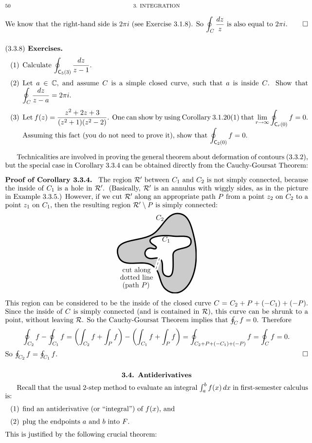
50 3. INTEGRATION
We know that the right-hand side is 2πi (see Exercise 3.1.8). So∮
C
dz
zis also equal to 2πi. □
(3.3.8) Exercises.
(1) Calculate∮
C5(3)
dz
z − 1.
(2) Let a ∈ C, and assume C is a simple closed curve, such that a is inside C. Show that∮C
dz
z − a= 2πi.
(3) Let f(z) =z2 + 2z + 3
(z2 + 1)(z2 − 2). One can show by using Corollary 3.1.20(1) that lim
r→∞
∮Cr(0)
f = 0.
Assuming this fact (you do not need to prove it), show that∮
C2(0)f = 0.
Technicalities are involved in proving the general theorem about deformation of contours (3.3.2),but the special case in Corollary 3.3.4 can be obtained directly from the Cauchy-Goursat Theorem:
Proof of Corollary 3.3.4. The region R′ between C1 and C2 is not simply connected, becausethe inside of C1 is a hole in R′. (Basically, R′ is an annulus with wiggly sides, as in the picturein Example 3.3.5.) However, if we cut R′ along an appropriate path P from a point z2 on C2 to apoint z1 on C1, then the resulting region R′ \ P is simply connected:
cut alongdotted line(path P )
C1
C2
This region can be considered to be the inside of the closed curve C = C2 + P + (−C1) + (−P ).Since the inside of C is simply connected (and is contained in R), this curve can be shrunk to apoint, without leaving R. So the Cauchy-Goursat Theorem implies that
∮C f = 0. Therefore∮
C2
f −∮
C1
f =(∫
C2
f +∫
Pf
)−(∫
C1
f +∫
Pf
)=∮
C2+P+(−C1)+(−P )f =
∮C
f = 0.
So∮C2
f =∮C1
f . □
3.4. AntiderivativesRecall that the usual 2-step method to evaluate an integral
∫ ba f(x) dx in first-semester calculus
is:
(1) find an antiderivative (or “integral”) of f(x), and
(2) plug the endpoints a and b into F .
This is justified by the following crucial theorem:

3.4. ANTIDERIVATIVES 51
(3.4.1) Fundamental Theorem of Calculus. If f is a continuous function on the interval [a, b],and F is any antiderivative of f (i.e., if F ′ = f), then∫ b
af(t) dt = F (b) − F (a).
The same is true in Complex Analysis:
(3.4.2) Theorem. Assume f is a continuous function on a region R, and C is a path in R fromsome point z1 to some point z2. If F is any antiderivative of f on R, then∫
Cf = F (z2) − F (z1).
(3.4.3) Note. In this case, the integral of f does not depend on the path from z1 to z2: the valueof the integral is F (z2) − F (z1), no matter what path from z1 to z2 is chosen.
(3.4.4) Example. Calculate∫C z3 dz, where C is any path from 0 to 1 + i.
Solution. F (z) = z4/4 is an antiderivative of z3 (on all of C), so∫C
z3 dz =z4
4
∣∣∣1+i
0=
(1 + i)4
4− 04
4=
−44
− 0 = −1. □
(3.4.5) Example. Let C be the upper half of the circle C2(0), oriented counterclockwise. In
Exercise 3.1.12(1), we calculated∫
C
z2 − 1z
dz by parametrizing the curve C. If we calculate theintegral by using antiderivatives, then there is no need to parametrize the curve:
Let
f(z) =z2 − 1
z= z − 1
zand F (z) =
z2
2− Log z,
where Log z is a branch of the logarithm function whose branch cut is the negative imaginary axis.(That is, we require ImLog z to be between −π/2 and +3π/2.) Then the branch cut misses thesemicircle traced out by C, so F is an antiderivative of f on C. Therefore, since C is a path from 2to −2, we have∫
C
z2 − 1z
dz = F (−2) − F (2) =(
(−2)2
2− Log(−2)
)−(
22
2− Log 2
)=(2 − (Log 2 + πi)
)−(2 − Log 2
)= −πi.
(3.4.6) Exercises.(1) Calculate
∫C
(ez + 1
z
)dz, where C is the lower half of the unit circle C1(0), oriented
counterclockwise.(2) Calculate
∫C sin z dz, where C(t) = log t + t3i for 1 ≤ t ≤ 2.
(3) Calculate∫C z−5 dz, where C is any path from −1 to 2 that does not pass through 0.
(3.4.7) Corollary. Assume f is a continuous function on a region R. If C is a closed path in R,and f has an antiderivative on R, then
∮C f = 0.
Proof. Let z0 be the starting point of C, so it is also the ending point, and let F be an antiderivativeof f . Then we see from Theorem 3.4.2 that∫
Cf = F (ending point) − F (starting point) = F (z0) − F (z0) = 0. □

52 3. INTEGRATION
(3.4.8) Remark. We saw in Example 3.1.7 that the integral of 1/z over the unit circle is not 0.Therefore, 1/z does not have an antiderivative on any (open) set that contains the unit circle. Sincethe integral of 1/z is log z, this implies that the log function cannot be consistently defined on theentire unit circle. This is another justification of the fact that the log function must have a branchcut.
Here is another part of the Fundamental Theorem of Calculus:(3.4.9) Recall. If f is continuous, and we define F (x) =
∫ xa f(t) dt, then F is an antiderivative
of f .A very similar fact is true in Complex Analysis (if we make an additional assumption):
(3.4.10) Theorem. Let f be a continuous function on a region R, and assume∮C f = 0 for every
closed curve in R. Fix some z0 ∈ R, and define
F (z) =∫
Cz
f , where Cz is any path from z0 to z.
Then F is an antiderivative of f .
Sketch of proof. First, note that F (z) depends only on z, not on the choice of the path Cz
(cf. Exercise 3.2.8). This means that F is a “well-defined” function. So we just need to show thatF ′ = f .
For each a ∈ R, we will show that |F ′(a) − f(a)| < ϵ for every ϵ > 0. This implies the desiredconclusion that F ′(a) = f(a) (see Exercise 3.4.11).
Assume that we are given some ϵ > 0. Since f is continuous, there is some δ > 0, such that|f(z) − f(a)| < ϵ whenever |z − a| < δ.
Since R is an open set, we may assume δ is small enough that Dδ(a) is contained in R. For h ∈ C,let Ca+h
a be the line segment from a to a + h.Note that if h is sufficiently close to 0, then Ca+h
a is contained in R. Therefore
F ′(a) = limh→0
F (a + h) − F (a)h
= limh→0
∫Ca+h
f −∫Ca
f
h= lim
h→0
∫Ca+h
af
h.
Also, for |h| < δ, and any z on Ca+ha , we have z ∈ Dδ(a), so |f(z) − f(a)| < ϵ. Therefore∣∣∣∣∫
Ca+ha
f(z) dz − f(a)h∣∣∣∣ = ∣∣∣∣∫
Ca+ha
(f(z) − f(a)
)dz
∣∣∣∣ ≤ maxz∈Ca+h
a
|f(z) − f(a)| · length(Ca+ha ) ≤ ϵ · |h|.
Dividing by |h||, we conclude that ∣∣∣∣∣∫Ca+h
af
h− f(a)
∣∣∣∣∣ < ϵ.
This means that limh→0
∫Ca+h
af
h = f(a), which completes the proof. □
(3.4.11) Exercise. Let w1, w2 ∈ C. Show that if |w1 − w2| < ϵ for every ϵ > 0, then w1 = w2.[Hint. If w1 = w2, let ϵ = |w1 − w2|/2.]
This has the following important consequence:(3.4.12) Exercise. Show that if f is holomorphic on a simply connected region R, then f has anantiderivative on R. [Hint. Cauchy-Goursat Theorem (3.2.7) and Theorem 3.4.10.]
We can now prove (a generalization of) Theorem 2.5.7:(3.4.13) Corollary. If u is a harmonic function on a simply connected region R, then u is the realpart of a holomorphic function on R.

3.5. CAUCHY INTEGRAL FORMULA 53
Proof. Let g = ux − iuy. Since u is harmonic, we have uxx = −uyy, so it is easy to verify that gsatisfies the Cauchy-Riemann equations:
(Re g)x = (ux)x = uxx = −uyy = (−uy)y = (Im g)y
and
(Re g)y = (ux)y = uyx = uxy = (uy)x = −(Im g)x.
So g is holomorphic.Therefore, we see from Exercise 3.4.12 that g has an antiderivative u + iv on R. Then u + iv is
holomorphic (because it has a derivative, namely g), so it satisfies the Cauchy-Riemann equations.In particular, we have uy = −vx, so
ux − iuy = ux + ivx = (u + iv)x = (u + iv)′ = g = ux − iuy,
so
ux = ux and uy = uy.
This means that u has the same partial derivatives as u (at all points of R), so u = u + C for someconstant C ∈ R. Then f = u + iv + C is holomorphic, and Re f = u + C = u. □
3.5. Cauchy Integral FormulaIt is easy to write down two different functions that have exactly the same values on the unit
circle C1(0), but have different values at 0. (E.g., let f1(x, y) = 1 and f2(x, y) = x2 + y2.) This isan illustration of the obvious fact that even if you know the value of a function at each point of aclosed curve, then you still may not be able to figure out what the value of the function is at anyof the points that are inside the curve.
The following astonishing theorem tells us that holomorphic functions do not behave this way:if you know the value of a holomorphic function at each point of a closed curve, then there is aformula to calculate the value of the function at each point that is inside the curve.
(3.5.1) Theorem (Cauchy Integral Formula). Assume• C is a (counterclockwise) simple, closed curve,• f is holomorphic on a region R that contains C and all points that are inside C, and• w is inside C.
Then
f(w) =1
2πi
∮C
f(z)z − w
dz.
(3.5.2) Example. Calculate∮
C
3z + 2z2 − 4
dz, whereC is the closed curve that is pictured at right.
2
C
Solution. We have3z + 2z2 − 4
=3z + 2
(z + 2)(z − 2)=
3z + 2z + 2
· 1z − 2
.
Therefore, if we let f(z) =3z + 2z + 2
, then 3z + 2z2 − 4
=f(z)z − 2
. Also note that f is holomorphiceverywhere except at −2, which is outside C, so f(z) is holomorphic on a region containing both C

54 3. INTEGRATION
and its inside. Therefore
∮C
3z + 2z2 − 4
dz =∮
C
f(z)z − 2
dz
= 2πi
(1
2πi
∮C
f(z)z − 2
dz
)= 2πi · f(2) (Cauchy Integral Formula, since 2 is inside C)
= 2πi · 3(2) + 22 + 2
= 4πi. □
(3.5.3) Example. Calculate∮
C
cos z
z(z − π2 )
dz for each of the following closed curves C:
(1) C (2) C
2
(3) C
2 4
Solution. (1) The integrand is holomorphic at all points except 0 and π/2 (the points wherethe denominator is 0), and neither of these points is inside C. Therefore, The Cauchy-GoursatTheorem tells us that the integral is 0.
(2) Let f(z) = (cos z)/(z − π/2). Then f is holomorphic at all points except π/2. Since π > 2,we have π/2 > 1, so it is clear from the picture that π/2 is outside the curve. Therefore, f isholomorphic at all points that are inside or on C. Hence
∮C
cos z
z(z − π2 )
dz =∮
C
cos z
z − π2
· 1z dz
=∮
C
f(z)z − 0
dz (definition of f(z), and z − 0 = z)
= 2πi f(0) (Cauchy Integral Formula, because 0 is inside C)
= 2πi
(cos 0
0 − π/2
)(definition of f(z))
= 2πi
(1−π
2
)(cos 0 = 1)
= −4i.
(3) Let f(z) = (cos z)/z. Then f is holomorphic at all points except 0. It is clear from thepicture that 0 is outside the curve, so f is holomorphic at all points that are inside or on C.

3.5. CAUCHY INTEGRAL FORMULA 55
Therefore∮C
cos z
z(z − π2 )
dz =∮
C
cos z
z· 1z − π
2
dz
=∮
C
f(z)z − π/2
dz (definition of f(z))
= 2πi f(π/2)(
Cauchy Integral Formula, because π/2 is inside C(since 1 ≤ π/2 ≤ 2)
)= 2πi
(cos(π/2)
π/2
)(definition of f(z))
= 2πi
(0
π/2
)(cos(π/2) = 0)
= 0. □
(3.5.4) Remark. The above method does not work when the inside of the curve contains morethan one pole of the integrand. In that situation, we will see in Chap. 5 that each pole inside thecurve contributes a certain amount to the integral, and this amount can be calculated by findingthe “residue” of the pole.
(3.5.5) Exercises. Calculate each of these contour integrals.
(1)∮
C1(0)
cos z
zdz,
(2)∮
C3(3)
exp(z)z − 5
dz
(3)∮
C3(3i)
exp(z)z − 5
dz
(4)∮
C4(2+i)
z2 + 1(z − 1)(z + 4)
dz,
(5)∮
C3(−3)
z2 + 1(z − 1)(z + 4)
dz,
(6)∮
C1(−2)
z3 + 1(z − 1)(z + 4)
dz,
(7)∮
C3(i)
z
z2 + 9dz,
(8)∮
C2(1)
z
z2 + 9dz,
(9)∮
C5(4−i)
z
z2 + 9dz,
Idea of proof of the Cauchy Integral Formula. Since w ∈ R and R is open, we haveDr(w) ⊆ R for some small r > 0 (see Exercise 1.3.6). Note that:
• f(z)z − w
is holomorphic in R ∖ {w}, and
• C can be deformed to Cr(w) in R ∖ {w},so
12πi
∮C
f(z)z − w
dz =1
2πi
∮Cr(w)
f(z)z − w
dz (deformation of contours (3.3.2))
=1
2πi
∫ 2π
0
f(w + reit)(w + reit) − w
ireit dt
parametrize Cr(w) by
z = w + reit (0 ≤ t ≤ 2π), sodz = (w + reit)′ dt
= (0 + reit · i) dt = ireit dt
=
12π
∫ 2π
0f(w + reit) dt
= average value of f on Cr(w)
→ f(w) as r → 0(
f is continuous, so f(z) ≈ f(w)for z ∈ Cr(w) if r ≈ 0
). □

56 3. INTEGRATION
(3.5.6) Remark (Mean Value Property). The Cauchy Integral Formula implies that the value of aholomorphic function at any point is equal to the average of its values on any circle that is centredat the point (and is such that the function is holomorphic on the circle and its inside points):
If f is holomorphic in an open set containing Dr(w), then
f(w) =12π
∫ 2π
0f(w + reit) dt.
Proof. We saw in the proof of the Cauchy Integral Formula that the right-hand side is equal to1
2πi
∮Cr(w)
f(z)z − w
dz. The Cauchy Integral Formula tells us that this is f(w). □
3.6. Cauchy Integral Formula for DerivativesThe Cauchy Integral Formula provides a formula for f . There is a very similar formula for the
derivative f ′, and even for the nth derivative f (n).
(3.6.1) Remark. Here is a non-rigorous derivation of the formula for f (n)(w) from the formula forf(w). We have:
f (n)(w) =dn
dwnf(w)
=dn
dwn
12πi
∮C
f(z)z − w
dz (Cauchy Integral Formula)
=1
2πi
∮C
∂n
∂wn
f(z)z − w
dz
(bring the derivativeinside the integral
)=
12πi
∮C
f(z)∂n
∂wn(z − w)−1 dz (f(z) is a constant for ∂/∂w)
=1
2πi
∮C
f(z) · 1 · 2 · 3 · · ·n · (z − w)−(n+1) dz
(∂
∂w(z − w)−r = r(z − w)−(r+1)
)=
n!2πi
∮C
f(z)(z − w)n+1
dz.
The above derivation is not a legitimate proof, because bringing a derivative into an integral isa step that needs further justification, but it does give the correct answer in this case:
(3.6.2) Theorem (Cauchy’s Integral Formula for derivatives). Assume
• C is a (counterclockwise) simple, closed curve,
• f is holomorphic on a region R that contains C and all points that are inside C, and
• w is inside C.
Then
f (n)(w) =n!2πi
∮C
f(z)(z − w)n+1
dz.
(3.6.3) Remark. The actual proof of Cauchy’s Integral Formula for derivatives is by inductionon n. Here is the case n = 1, but assuming, for simplicity, that w = 0. (The general case is similar,

3.6. CAUCHY INTEGRAL FORMULA FOR DERIVATIVES 57
and is left as an exercise for students who are interested.) We have
f ′(0) = limh→0
f(0 + h) − f(0)h
= limh→0
1h
(f(h) − f(0)
)=
12πi
limh→0
1h
∮C
(f(z)z − h
− f(z)z − 0
)dz (Cauchy Integral Formula)
=1
2πilimh→0
∮C
f(z)z(z − h)
dz
(f(z)z − h
− f(z)z
=z f(z) − (z − h) f(z)
z(z − h)=
h f(z)z(z − h)
).
So∣∣∣∣f ′(0) − 12πi
∮C
f(z)z2
dz
∣∣∣∣ = ∣∣∣∣ 12πi
limh→0
∮C
(f(z)
z(z − h)− f(z)
z2
)dz
∣∣∣∣=∣∣∣∣ 12πi
limh→0
∮C
f(z)z2(z − h)
h dz
∣∣∣∣≤ 1
2π· length C · lim
h→0maxz∈C
∣∣∣∣ f(z)z2(z − h)
∣∣∣∣ · |h| (Lemma 3.1.14)
≤ 12π
· length C · maxz∈C
2|f(z)||z|3
· limh→0
h
(h ≈ 0 ⇒ |h| < |z|/2⇒ |z − h| > |z|/2
)≤ 1
2π· length C · M · 0
(for some constant M , by
Heine-Borel (see 3.1.20(1))
)= 0.
(3.6.4) Example. Calculate∮
C1(0)
exp(z)(z − 1)k
dz for k = 0, 1, 2, 3.
Solution. Let f(z) = ez, so f(z) is entire. Also note that:
• 0 is inside C1(0), and
• f (k)(z) = f(z) for all k.
We now calculate the integral for each value of k in turn.
• For k = 0, the integrand exp(z)(z − 1)0
= ez is entire, so the Cauchy-Goursat Theorem tells usthat ∮
C1(0)
exp(z)(z − 1)0
dz = 0.
• For k = 1, we have∮C1(0)
exp(z)z − 1
dz =∮
C1(0)
f(z)z − 1
dz
= 2πi · f(1) (Cauchy Integral Formula)= 2πi · e1 (f(z) = ez)= 2πei.

58 3. INTEGRATION
• For k = 2, we have∮C1(0)
exp(z)(z − 1)2
dz =∮
C1(0)
f(z)(z − 1)2
dz
= 2πi · f ′(1) (Cauchy Integral Formula for derivatives)= 2πi · e1 (f (k)(z) = f(z) for all k)= 2πei.
• For k = 3, we have∮C1(0)
exp(z)(z − 1)3
dz =∮
C1(0)
f(z)(z − 1)3
dz
=2πi
2!· f ′′(1) (Cauchy Integral Formula for derivatives)
= πi · e1 (f (k)(z) = f(z) for all k)= πei. □
(3.6.5) Example. Calculate∮
C5(2)
z2 + 3(z − 1)n
dz for all n ≥ 0.
Solution. Let f(z) = z2 + 3, and note that 1 is inside the curve of integration C5(2).
• f ′′(z) = 2, and
• f (n)(z) = 0 for all n ≥ 3.
We now calculate the integral for each value of n.
• For n = 0, the integrand z2 + 3(z − 1)0
= z2 + 3 is entire, so the Cauchy-Goursat Theorem tells usthat ∮
C1(0)
z2 + 3(z − 1)0
dz = 0.
• For n = 1, we have∮C5(2)
z2 + 3z − 1
dz =∮
C5(2)
f(z)z − 1
dz
= 2πi · f(1) (Cauchy Integral Formula)= 2πi · (12 + 3) (f(z) = z2 + 3)= 8πi.
• For n = 2, we have∮C5(2)
z2 + 3(z − 1)2
dz =∮
C5(2)
f(z)(z − 1)2
dz
= 2πi · f ′(1) (Cauchy Integral Formula for derivatives)
= 2πi · (2 · 3)(
f ′(z) =d
dz(z2 + 3) = 2z
)= 12πi.

3.6. CAUCHY INTEGRAL FORMULA FOR DERIVATIVES 59
• For n = 3, we have∮C5(2)
exp(z)(z − 1)3
dz =∮
C5(2)
f(z)(z − 1)3
dz
=2πi
2!· f (2)(1) (Cauchy Integral Formula for derivatives)
= πi · 2(
f ′′(z) =d
dzf ′(z) =
d
dz2z = 2
)= 2πi.
• Finally, for n ≥ 4, we have∮C5(2)
exp(z)(z − 1)n
dz =∮
C5(2)
f(z)(z − 1)n
dz
=2πi
(n − 1)!· f (n−1)(1) (Cauchy Integral Formula for derivatives)
=2πi
(n − 1)!· 0
(f (n−1)(z) =
d
dz(constant) = 0 for n ≥ 4
)= 0. □
(3.6.6) Exercises. Calculate these contour integrals.(1)
∮C3(1)
ez
z4dz,
(2)∮
C1(3)
Log z
(z − e)3dz,
(3)∮
C2(i)
cos z
z2dz,
(4)∮
C2(i)
cos z
z2 ezdz,
(5)∮
C4(0)
z3 − 2z2 + z
(z − 2)kdz,
for k = 0, 1, 2, 3.
We conclude this section with an example that illustrates how we will deal with functions thathave more than one pole inside the contour of integration.
(3.6.7) Example. Calculate∮
C5(2)
z2 + 1z(z − 4)2
dz.
Solution. The integrand is holomorphic everywhere except 0 and 4, but both of those points areinside the curve of integration. To deal with this, we add an additional path P that separates 0from 4, and divides the original closed curve into two parts C1 and C2:
P
C1 C2
0 4
Combining C1 and C2 with P yields closed curves C∗1 and C∗
2 . Notice that C1 and C2 traverse P inopposite directions (more precisely, we have C∗
1 = C1 + P and C∗2 = C2 + (−P )), so the integrals
over P will cancel if we integrate over both C∗1 and C∗
2 . Indeed:∮C5(2)
f =∫
C1
f +∫
C2
f =(∫
C1
f +∫
Pf
)+(∫
C2
f −∫
Pf
)=∮
C1+Pf +
∮C2+(−P )
f =∮
C∗1
f +∮
C∗2
f.

60 3. INTEGRATION
Now, we have∮C∗
1
z2 + 1z(z − 4)2
dz =∮
C∗1
(z2 + 1)/(z − 4)2
z − 0dz
= 2πi · z2 + 1(z − 4)2
∣∣∣∣z=0
Cauchy Integral Formula,
since z2 + 1(z − 4)2
is holomorphicinside (and on) C∗
1 , and 0 is inside C∗1
= 2πi · 02 + 1
(0 − 4)2
=18πi.
Also:∮C∗
2
z2 + 1z(z − 4)2
dz =∮
C∗2
(z2 + 1)/z
(z − 4)2dz
= 2πi
(z2 + 1
z
)′∣∣∣∣∣z=4
Cauchy Integral Formula for derivatives,
since z2 + 1z
is holomorphicinside (and on) C∗
2 , and 4 is inside C∗2
= 2πi
(z2 − 1
z2
)∣∣∣∣z=4
(
z2 + 1z
)′=
(z2 + 1)′z − (z2 + 1)z′
z2
=(2z + 0)z − (z2 + 1) · 1
z2=
z2 − 1z2
= 2πi
(42 − 1
42
)=
158
πi.
Therefore ∮C5(2)
z2 + 1z(z − 4)2
dz =∮
C∗1
z2 + 1z(z − 4)2
dz +∮
C∗2
z2 + 1z(z − 4)2
dz
=18πi +
158
πi
= 2πi. □
3.7. Consequences of the Cauchy Integral FormulasExamples (and exercises) in the preceding two sections demonstrated that the Cauchy Integral
Formulas can be used to calculate integrals. These are very practical applications of the formulas.In this section, we will see that the formulas also have important theoretical consequences.
It is a basic fact of trigonometry that |sin x| ≤ 1, so the function sin x is bounded on all of R.Also, the sine function is differentiable everywhere. However, there is no such function in complexanalysis:
(3.7.1) Theorem (Liouville’s Theorem). Every bounded, entire function is constant.

3.7. CONSEQUENCES OF THE CAUCHY INTEGRAL FORMULAS 61
Proof. Let f be an entire function that is bounded. Then, for w ∈ C, and r > 0, the CauchyIntegral Formula for derivatives tells us
f ′(w) =1
2πi
∮Cr(0)
f(z)(z − w)2
dz.(∗)
This is true for every r, so it remains true as r → ∞:
|f ′(w)| =12π
limr→∞
∣∣∣∣∣∮
Cr(0)
f(z)(z − w)2
dz
∣∣∣∣∣ (apply limr→∞
to both sides of (∗))
≤ 12π
· limr→∞
M(r − |w|
)2 · length(Cr(0)
) Lemma 3.1.14 and f is bounded(so |f(z)| ≤ M for some constant M), and|z − w| ≥ |z| − |w| by Triangle Inequality
= lim
r→∞
M
r − |w|· lim
r→∞
r
r − |w|(length
(Cr(0)
)= 2πr)
= 0 · 1= 0.
Since this is true for all w ∈ C, we conclude that f is constant (see Exercise 2.3.10). □
(3.7.2) Exercises.
(1) The function sin z is entire, but not constant, so it must be unbounded on C (even though|sin x| ≤ 1 for all real x). Verify this explicitly, by showing that limn→∞ |sin(n i)| = ∞.
(2) Show that if f is entire, and Re f is bounded, then f is constant.[Hint. Show that Liouville’s Theorem applies to the function exp f(z).]
(3) Let f be an entire function, and assume there is some open disk Dr(a) (with r > 0), suchthat f(z) /∈ Dr(a), for all z ∈ C. Show that f is constant.[Hint. Show that Liouville’s Theorem applies to the function 1/
(f(z) − a
).]
(4) Show that if f is entire, and there is a constant M , such that |f | ≤ |z| + M , for all z ∈ C,then f is a linear function: there exist a, b ∈ C, such that f(z) = az + b for all z ∈ C.[Hint. For all w ∈ C, show that lim
r→∞
∮Cr(0)
f(z)(z − w)2
dz = 0. Conclude from Cauchy’s Integral Formula
for derivatives that f ′′(w) = 0.]
(5) Let f be an entire function. Show that if |f(z)| ≤ |z|3 for all z ∈ C, then f is a polynomialof degree ≤ 3.
Here is an important consequence of Liouville’s Theorem that was already mentioned inRemark 1.1.42:
(3.7.3) Theorem (Fundamental Theorem of Algebra). Every nonconstant polynomial has a rootin C.
The proof requires a lemma:
(3.7.4) Lemma. If P (z) is a nonconstant polynomial, then limz→∞ |P (z)| = ∞.

62 3. INTEGRATION
Proof. Write P (z) =∑n
k=0 akzk, with an = 0. Then
|P (z)| =∣∣a0 + a1z + a2z
2 + · · · + anzn∣∣
= |z|n ·∣∣∣∣a0 + a1z + a2z
2 + · · · + anzn
zn
∣∣∣∣= |z|n ·
∣∣∣a0
zn+
a1
zn−1+
a2
zn−2+ · · · + an−1
z+ an
∣∣∣→ ∞ · |0 + 0 + · · · 0 + an| (as z → ∞)= ∞ (an = 0). □
Proof of the Fundamental Theorem of Algebra. We prove the contrapositive: we show thatevery polynomial with no roots is constant.
Given any polynomial P (z), let f(z) = 1/P (z), so f(z) is a rational function, which impliesthat it is holomorphic everywhere that the denominator is not zero. If P (z) has no roots, then thismeans that f(z) is entire.
Also, the lemma implies that f(z) is bounded. To see this, note that the lemma tells us there issome R > 0, such that |P (z)| is very large whenever |z| > R. In particular, we must have |f(z)| > 1whenever |z| > R. This implies
|f(z)| =1
|P (z)|< 1 whenever |z| > R.
However, we know from the Heine-Borel Theorem that there is some M > 0, such that |f(z)| < Mwhenever |z| ≤ R (see Corollary 3.1.20(2)). Hence, we have |f(z)| ≤ max(1,M) for all z. Thismeans that f(z) is bounded, as claimed.
Now, since f(z) is a bounded entire function, we conclude from Liouville’s Theorem that f(z)is constant. So P (z) = 1/f(z) is also constant. □
(3.7.5) Remark. The Fundamental Theorem of Algebra implies that every polynomial of degree nhas exactly n roots (counting multiplicity), if n > 0.
In ordinary calculus, there are many functions that are differentiable, but do not have a secondderivative (or that have a second derivative, but not a third derivative, etc.). For example, x4/3 isdifferentiable on R, but the second derivative (x4/3)′′ does not exist at 0. But this never happensfor holomorphic functions:
(3.7.6) Corollary. If f is holomorphic in R, then f (n)(z) exists for all n ≥ 0 (and all z ∈ R).
Proof. If f is holomorphic, then the Cauchy Integral Formula for derivatives provides an explicitformula for f (n)(z). This is much more than just saying that the derivative exists. □
Not only does the nth derivative exist, but the Cauchy Integral Formula for derivatives can beused to obtain a bound on how large it is:
(3.7.7) Exercise (Cauchy’s Inequality). Assume f is holomorphic on a region R that contains theclosed disk Dr(a) (with r > 0), and let M ∈ R+. Show that if |f(z)| ≤ M for all z ∈ Cr(a), then
|f (n)(a)| ≤ n! Mrn
.
(3.7.8) Exercise (Harmonic functions are infinitely differentiable). Show that if u is a harmonicfunction on a region R, then then u(n)(z) exists for all n ≥ 0 (and all z ∈ R).[Hint. Corollaries 3.4.13 and 3.7.6.]
Corollary 3.7.6 also implies the following famous converse to the Cauchy-Goursat Theorem:

3.7. CONSEQUENCES OF THE CAUCHY INTEGRAL FORMULAS 63
(3.7.9) Corollary (Morera’s Theorem). If f is continuous in the region R, and∮C f = 0 for every
closed curve C in R, then f is holomorphic in R.
Proof. We know from Theorem 3.4.10 that f has an antiderivative F on R. This means thatF ′ = f . We also know from Corollary 3.7.6 that F ′ is differentiable, or, in other words, that F ′ isholomorphic. Since F ′ = f , this means that f is holomorphic. □


CHAPTER 4
Power Series
4.1. Review of sequences and series§4.1A. Sequences.
(4.1.1) Recall. Suppose (ak) = (a1, a2, a3, . . .) is a sequence of numbers. We say that the sequence{ak} converges to L (and we may write ak → L or lim
k→∞ak = L) if ak is close to L whenever k is
large.
In ordinary calculus, each ak is a real number, but the same idea works for complex numbers.Here is the formal definition:
(4.1.2) Definition. limk→∞
ak = L if ∀ϵ > 0, ∃N ∈ N, ∀k ≥ N , |ak − L| < ϵ.
(4.1.3) Key Fact. If limk→∞
ak = L and f is continuous at L, then limk→∞
f(ak) = f(L).
Informal justification. If k is large, then ak is close to L (because ak → L). This implies thatf(ak) is close to f(L) (because f is continuous at L). □
(4.1.4) Example. If limk→∞
ak = L, then limk→∞
a2k = L2 and lim
k→∞|ak| = |L|, because z2 and |z| are
continuous functions.
(4.1.5) Exercise. Prove Key Fact 4.1.3, using the official definitions (2.2.1, 2.6.2, and 4.1.2).
§4.1B. Order of magnitude. In this section, we assume k is very large. Then√
k < k < k2, and,in later sections, it will be important to be able to determine the relative sizes of other sequencesthat arise.
L’Hôpital’s Rule is sometimes helpful for this.
(4.1.6) Recall (L’Hôpital’s Rule). Assume f(x) and g(x) are differentiable. If either
limx→∞
f(x) = limx→∞
g(x) = 0 or limx→∞
f(x) = limx→∞
g(x) = ∞,
then
limx→∞
f(x)g(x)
= limx→∞
f ′(x)g′(x)
.
(4.1.7) Example. If k is very large, then which is larger: k100 or ek ?65

66 4. POWER SERIES
Solution. We have
limk→∞
k100
ek= lim
x→∞
x100
ex
= limx→∞
d100
dx100x100
d100
dx100ex
(apply L’Hôpital’s Rule 100 times)
= limx→∞
100!ex
( d
dxxn = nxn−1 and d
dxex = ex
)=
100!∞
(ex → ∞ as x → ∞)
= 0.
So k100 is (much) smaller than ek. □
In the following notation, this means k100 ≪ ek:
(4.1.8) Notation. Writing ak ≪ bk (or bk ≫ ak) means ak/bk → 0 as k → ∞.
The above example is a special case of the general fact that exponential functions are muchlarger than polynomials (if the base of the exponent is greater than 1):
(4.1.9) Example. If a and b are constants, with b > 1, then ka ≪ bk.
And logarithms are much smaller than (positive) powers:
(4.1.10) Exercises.
(1) Show that if a > 0, then log k ≪ ka. [Hint. L’Hôpital’s Rule.]
(2) Show k1/k → 1 as k → ∞. [Hint. What is the limit of log k1/k ?]
(4.1.11) Example. Since√
k = k1/2, Exercise 4.1.10(1) implies that log k ≪√
k.
Sometimes, it is necessary to consider expressions where both the base and the exponent arenot constant:
(4.1.12) Example. Calculate limk→∞
(1 +
1k
)k.

4.1. REVIEW OF SEQUENCES AND SERIES 67
Solution. To eliminate the exponent, we take a logarithm:
limk→∞
log(
1 +1k
)k= lim
k→∞k log
(1 +
1k
)= lim
k→∞
log(1 + k−1)k−1
= limx→∞
log(1 + x−1)x−1
= limx→∞
d
dxlog(1 + x−1)
d
dxx−1
(L’Hôpital’s Rule)
= limx→∞
1(1 + x−1)
· (0 − x−2)
−x−2
(Chain Rule to calculate thederivative of the numerator
)= lim
x→∞
1
1 +1x
=1
1 + 0
(lim
x→∞
1x
= 0)
= 1.
Therefore, we have (1 +
1k
)k= exp log
(1 +
1k
)k4.1.3−→ exp 1 = e. □
Some sequences, such as factorials, do not yield easily to L’Hôpital’s Rule (e.g., because theycannot easily be viewed as differentiable functions), so other methods are also necessary.
(4.1.13) Example. If k is very large, then which is larger: k! or 100k ?
Solution. First, we note that if n = 1002/2, then (2n)! > 1002n:(2n)! = 1 · 2 · 3 · · · 2n
= 4! ·(5 · 6 · · · · n
)·((n + 1) · (n + 2) · · · (2n)
)> 24 · 2n−4 · nn
4! = 24 > 16 = 24,k > 2 for k > 4,and n + k > n
= (2n)n
= (1002)n (n = 1002/2)= 1002n.
Thus, we havek! = 1 · 2 · 3 · · · k
= (2n)! · (2n + 1) · (2n + 2) · · · k
> (2n)! · 100k−2n (2n > 100, because n = 1002/2)> 1002n · 100k−2n ((2n)! > 1002n from above)= 100k. □

68 4. POWER SERIES
In fact, a similar argument shows that k! is much larger than any exponential function (whenk is large):
(4.1.14) Example. For every constant c, we have k! ≫ ck.
(4.1.15) Corollary. limk→∞
k√
k! = ∞.
Proof. For any constant c, we have k! > ck when k is large. By taking the kth root of both sides,we conclude that k
√k! > c. Since c is arbitrary, we conclude that k
√k! → ∞. □
It is clear that k! = 1 · 2 · 3 · · · k is smaller than k · k · k · · · k = kk. The following observationshows that it is much smaller (i.e., k! ≪ kk):
(4.1.16) Fact (Stirling’s Formula). k! is approximately√
2πkkk
ek. More precisely, we have
limk→∞
k!√
2πkkk
ek
= 1.
Idea of proof. We establish only a rough estimate of k!, which omits the factor√
2πk. To dothis, we need to calculate the product k! = 1 · 2 · 3 · · · k, but we will convert it to a sum (which iseasier to calculate), by taking a logarithm:
log k! = log(1 · 2 · 3 · · · k)= log 1 + log 2 + · · · + log k
≈∫ k
1log x dx (Integral Test from ordinary calculus)
= (x log x − x)∣∣k1
(Integrate by parts with u = log x and dv = dx)= (k log k − k) − (1 · log 1 − 1)≈ k log k − k.
Therefore, a rough estimate of the size of k! is given by
k! = exp log k! ≈ exp(k log k − k) =kk
ek. □
(4.1.17) Exercise. Arrange the following in order from smallest to largest. (Assume that k is verylarge.) There is no need to show your work.
kk, 3k,2k
k!,
(1 +
1k
)k,
k√
2, 2, k, log k, k2,√
k, kk2,
110k
,
2k,k√
k,k
log k,
2k + 1k + 1
,k2 + 1k + 1
,√
k + 1 −√
k, k!, k√
k!, 2k! .
§4.1C. Series. The difference between a sequence and a series is that a series is the sum of thenumbers in a sequence:
(4.1.18) Definition. Suppose∑∞
k=0 ak = a0 + a1 + a2 + a3 + · · · is an infinite series.• We say
∑∞k=0 ak = L if
∑nk=0 ak → L as n → ∞. In this case, we say that L is the sum of
the series.• We say
∑∞k=0 ak converges if
∑∞k=0 ak = L for some L ∈ C.
• We say∑∞
k=0 ak converges absolutely if∑∞
k=0 |ak| converges.

4.1. REVIEW OF SEQUENCES AND SERIES 69
• We call∑n
k=0 ak the nth partial sum of the series.• A series that does not converge is said to diverge.
(4.1.19) Exercises.(1) (nth term test) Show that if
∑∞k=0 ak converges, then lim
k→∞ak = 0.
[Hint. If∑n−1
k=0 ak and∑n
k=0 ak are both close to L, then what can you say about an?]
(2) (Geometric Series) For a, z ∈ C (with a = 0), show that∑∞
k=0 azk converges iff |z| < 1.
Furthermore, show that if the series does converge, then∞∑
k=0
azk =a
1 − z.
[Hint. The (contrapositive of the) nth term test applies when |z| ≥ 1. For the other direction (and tocalculate the sum of the series), simplify the expression (1 + z + · · · + zn)(1 − z).]
(4.1.20) Warning. The converse of the nth term test is false. For example,1k→ 0, but
∞∑k=0
1k
does not converge.
More precisely, this sum (which is called the Harmonic series) is ∞. This follows from theIntegral Test (if you remember that from ordinary calculus), or you can see this by observing that:
∞∑k=0
1k
= 1 +12
+13
+14
+15
+16
+17
+18
+19
+ · · · + 116
+ · · ·(
we underline some termsto group them together
)> 1 +
12
+14
+14
+18
+18
+18
+18
+116
+ · · · + 116
+ · · ·
= 1 +12
+ 2 · 14
+ 4 · 18
+ 8 · 116
+ 16 · 132
+ 32 · 164
+ · · ·
= 1 +12
+12
+12
+12
+12
+12
+ · · ·
= ∞.
(4.1.21) Facts.(1) If a series converges absolutely, then it converges:
If∑∞
k=0 |ak| converges, then∑∞
k=0 ak converges.
(2) (Comparison Test) If∑∞
k=0 |bk| converges, and |ak| ≤ |bk| for all sufficiently large k, then∑∞k=0 ak converges (absolutely).
The following conclusions can be obtained by comparing with a geometric series:
(4.1.22) Corollary.(1) (Ratio Test) If lim
k→∞|ak+1/ak| < 1, then
∑∞k=0 ak converges absolutely.
Furthermore, if limk→∞
|ak+1/ak| > 1, then∑∞
k=0 ak does not converge.
(2) (Root Test) If limk→∞
k√|ak| < 1, then
∑∞k=0 ak converges absolutely.
Furthermore, if limk→∞
k√
|ak| > 1, then∑∞
k=0 ak does not converge.
(4.1.23) Warning. If limk→∞
|ak+1/ak| = 1 (or does not exist), then the Ratio Test does not tell you
anything. Similarly, if limk→∞
k√
|ak| = 1 (or does not exist), then the Root Test does not tell youanything. The series might converge, or it might not.

70 4. POWER SERIES
4.2. Power series(4.2.1) Definition. A power series centred at z0 is a series of the form
∑k≥0 ck(z − z0)k.
(4.2.2) Remark. For the important special case where z0 = 0, this simplifies to∑
k≥0 ck zk.
(4.2.3) Exercises. Use the Ratio Test to show that each of these series converges for the specifiedvalues of z. (But you do not need to show that the sum is equal to the given function.)
11 − z
= 1 + z + z2 + z3 + · · · =∑
k≥0zk if |z| < 1.(1)
ez = 1 + z +z2
2!+
z3
3!+ · · · =
∑k≥0
zk
k!for all z ∈ C.(2)
cos z = 1 − z2
2!+
z4
4!− z6
6!± · · · =
∑k≥0
(−1)k z2k
(2k)!for all z ∈ C.(3)
sin z = z − z3
3!+
z5
5!− z7
7!± · · · =
∑k≥0
(−1)k z2k+1
(2k + 1)!for all z ∈ C.(4)
(4.2.5) Exercise. Suppose∑
k≥0 ck (w − z0)k converges, and |z − z0| < |w − z0|. Show that∑k≥0 ck (z − z0)k converges absolutely.
Hint. Since∑
k≥0 ck(w − z0)k converges, the nth term test implies lim ck(w − z0)k = 0.Therefore lim |ck(w − z0)k| = 0 (why?), so |ck(w − z0)k| < 1 for all large k. Hence, lettingr = |z − z0|/|w − z0| < 1, we have
|ck(z − z0)k| = |ck(w − z0)k| · rk < 1 · rk < rk (for all large k).So you can compare
∑k≥0 ck(z − z0)k with the geometric series
∑k≥0 rk. □
This has the following very important consequence:
(4.2.6) Theorem. Every power series has a radius of convergence:If∑
k≥0 ck(z − z0)k is a power series, then there exists R ∈ [0,∞], such that the series:• converges absolutely whenever |z − z0| < R (i.e., z ∈ DR(z0)), but• diverges whenever |z − z0| > R (i.e., z /∈ DR(z0)).
(4.2.7) Definition. The number R of Theorem 4.2.6 is called the radius of convergence of thepower series.
(4.2.8) Example. From Exercise 4.2.3 (and the nth term test), we see that the radius of convergenceof the power series for 1/(1 − z) is 1, but for ez, cos z, and sin z, the radius of convergence of thepower series is ∞.
(4.2.9) Example. What is the radius of convergence of the power series∑
k≥0
k2(z − 3)k
7k?
Solution. We use the Ratio Test:∣∣∣∣(k + 1)2(z − 3)k+1
7k+1
∣∣∣∣/∣∣∣∣k2(z − 3)k
7k
∣∣∣∣ = (k + 1)2
k2· |z − 3|
7→ 1 · |z − 3|
7=
|z − 3|7
.
If |z − 3| < 7, then this limit is less than 1, so the power series converges (by the Ratio Test); butif |z − 3| > 7, then the limit is greater than 1, so the power series diverges (by the Ratio Test).Therefore, the radius of convergence is 7. □

4.2. POWER SERIES 71
Alternate solution (using the Root Test):
k
√∣∣∣∣k2(z − 3)k
7k
∣∣∣∣ = k√
k2 · |z − 3|7
→ 1 · |z − 3|7
=|z − 3|
7.
If |z − 3| < 7, then this limit is less than 1, so the power series converges (by the Root Test); butif |z − 3| > 7, then the limit is greater than 1, so the power series diverges (by the Root Test).Therefore, the radius of convergence is 7. □
(4.2.10) Exercise. Use the Ratio Test to find the radius of convergence of each power series.(1)
∑k≥0 2k(z − 5)k.
(2)∑
k≥0
k3(z + 2)k
k + 1.
(3)∑
k≥0 k! (z − a)k.
(4)∑
k≥0
k! (z − 3)k
kk.
(4.2.11) Exercise. Show:
the radius of convergence of∑k≥0
ck(z − z0)k is 1lim
k→∞k√|ck|
if the limit exists. (We use the convention that 1/∞ = 0 and 1/0 = ∞.) [Hint. Root Test.]
(4.2.12) Example. What is the radius of convergence of∑
k≥0
(3k + 14k − 5
)k(z − 2)k ?
Solution. We have
k
√(3k + 14k − 5
)k=
3k + 14k − 5
=3 + 1
k
4 − 5k
→ 3 + 04 − 0
=34,
so the radius of convergence is 13/4
= 4/3 (by Exercise 4.2.11). □
(4.2.13) Example. What is the radius of convergence of∑
k≥0
(3k + 14k − 5
)k2
(z − 2)k ?
Solution. We have k
√(3k + 14k − 5
)k2
=(
3k + 14k − 5
)k=
(3 + 1
k
4 − 5k
)k
≈(
34
)k→ 0, so the radius of
convergence is 10
= ∞ (by Exercise 4.2.11). □
(4.2.14) Remark. Many of the power series that appear in later sections have factorials in theircoefficients (because they are Taylor series). In order to apply Exercise 4.2.11 (or the Root Test),it is therefore important to remember (at least) the weak version of Stirling’s Formula that is atthe end of the proof of Fact 4.1.16: k! ≈ kk/ek.
(4.2.15) Exercise. Use Exercise 4.2.11 (or the Root Test) to find the radius of convergence of eachpower series in Exercise 4.2.10.
If a function is holomorphic on a disk, then its “Taylor series” converges at every point of thedisk:
(4.2.16) Exercise. Show that if f is holomorphic on DR(z0), then the radius of convergence of the
power series∑
k≥0
f (k)(z0) (z − z0)k
k!is at least R. [Hint. Cauchy’s Inequality (3.7.7).]
72 4. POWER SERIES
(4.2.17) Exercise. Show that the radius of convergence of any power series∑
k≥0 ck(z−z0)k is thesame as the radius of convergence of its differentiated power series
∑k≥0 k ck(z − z0)k−1.
Hint. To simplify the notation, you may assume that z0 = 0, so the power series is∑
k≥0 ckzk. Let R be itsradius of convergence. And let R′ be the radius of convergence of the differentiated series.
For any fixed z, note that |ckzk| ≤ |kckzk−1| for all large k. Therefore, if∑
k≥0 k ckzk−1 converges absolutely,then
∑k≥0 ckzk also converges absolutely, by the Comparison Test. From this, conclude that R ≥ R′.
For the opposite inequality, suppose z ∈ DR(0), and choose r, such that |z| < r < R. Then |z/r| < 1, so|k ckzk−1| ≤ |ckrk| for all large k. (Why?) Also, the series
∑k≥0 ckrk converges absolutely. (Why?) So the
Comparison Test implies that∑
k≥0 k ckzk−1 converges. □
(4.2.18) Warning. Theorem 4.2.6 does not say anything about what happens when |z − z0| = R(see Warning 4.1.23). It turns out that some power series converge at all of the points of CR(z0),others converge at none of the points on this circle, and many are somewhere in between.
4.3. Power series and holomorphic functionsEvery holomorphic function is given by a power series:
(4.3.1) Theorem. If f is holomorphic on Dr(z0), then there is a power series∑
k≥0 ck(z − z0)k,such that f(z) =
∑k≥0 ck(z − z0)k for all z ∈ Dr(z0).
In fact, ck =f (k)(z0)
k!, so f is equal to its Taylor series.
Idea of proof. To simplify the notation, let us assume that z0 = 0. For z ∈ Dr(0), we wish toshow f(z) =
∑k≥0 ckz
k, where ck = f (k)(0)/k!. However, the notation works out a bit better if wechange z to w:
For w ∈ Dr(0), we wish to show f(w) =∑
k≥0
f (k)(0)k!
wk.
4.3. POWER SERIES AND HOLOMORPHIC FUNCTIONS 73
Since |w| < r, we may choose some r′, such that |w| < r′ < r. Then we have
f(w) =1
2πi
∮Cr′ (0)
f(z)z − w
dw (Cauchy Integral Formula)
=1
2πi
∮Cr′ (0)
f(z)z
· 11 − (w/z)
dz (factor out z in the denominator)
=1
2πi
∮Cr′ (0)
f(z)z
·∑k≥0
(w
z
)kdz
(Geometric Series with |w/z| = |w|/r′ < 1
(since w ∈ Dr′(0) and z ∈ Cr′(0))
)
=1
2πi
∮Cr′ (0)
∑k≥0
f(z)z
·(w
z
)kdz
=∑k≥0
12πi
∮Cr′ (0)
f(z)z
·(w
z
)kdz
The integral of a sum is the sum of the integrals.
However, that is for finite sums.It is not always true for infinite sums, so
this step needs justification (which we omit).
=∑k≥0
wk · 12πi
∮Cr′ (0)
f(z)zk+1
dz
(the variable of integration is z, so wk is a constant
and can therefore be pulled out of the integral
)=∑k≥0
wk · 1k!
f (k)(0)(Cauchy Integral Formula for derivatives
)=∑k≥0
f (k)(0)k!
wk. □
The above theorem tells us that every holomorphic is given by a power series. Actually, however,there is not just one power series: there will (usually) be a different power series at each point ofthe domain of f .
Conversely, every (convergent) power series defines a holomorphic function:
(4.3.2) Theorem. If R is the radius of convergence of the power series∑
k≥0 ck(z − z0)k, thenf(z) =
∑k≥0 ck(z − z0)k is holomorphic on Dr(z0).
Furthermore, term-by-term differentiation of the power series yields f ′:f ′(z) =
∑k≥0
k ck(z − z0)k−1 for z ∈ Dr(z0).
We will omit the proof of this theorem.
(4.3.3) Exercise. Let R be the radius of convergence of the Taylor series∑
k≥0 ck(z − z0)k of aholomorphic function f . Show that f is holomorphic on DR(z0), but is not holomorphic on anylarger open disk that is centred at z0.Hint. From Theorems 4.3.1 and 4.3.2, we know that f(z) =
∑k≥0 ck(z − z0)k is holomorphic on DR(z0).
Exercise 4.2.16 implies that it cannot be holomorphic on any larger disk. □
This means that the radius of convergence of the Taylor series for f at z0 is the distance from z0
to the nearest point at which f is not holomorphic (and cannot be extended to be holomorphic).In particular, if f is entire, which means there are no points at which it is not holomorphic, thenthe Taylor series converges everywhere, so the radius of convergence is ∞.
(4.3.4) Example. What is the radius of convergence of the Taylor series for f(z) =ez
z − 3at 4i?

74 4. POWER SERIES
Solution. f is holomorphic everywhere except at z = 3. (And f is definitely not holomorphicat 3, because it has a pole there.) Since the distance from 4i to 3 is |3 − 4i| =
√32 + 42 = 5, we
conclude that the radius of convergence of the Taylor series is 5. □
(4.3.5) Example. (a) Find the first four terms of the Taylor series for f(z) = z1/2, centred at 1.(b) Also find the radius of convergence of the Taylor series.
Solution. (a) We have:f(z) = z1/2 so f(1) = 1, and
f ′(z) =12z−1/2 so f ′(1) =
12, and
f ′′(z) =12
(−1
2z−3/2
)= −1
4z−3/2 so f ′′(1) = −1
4, and
f ′′′(z) = −14
(−3
2z−5/2
)=
38z−5/2 so f ′′′(1) =
38.
Therefore, the Taylor series is
f(z) = 1 +12(z − 1) − 1
4· (z − 1)2
2!+
38· (z − 1)3
3!+ · · ·
= 1 +12(z − 1) − 1
8(z − 1)2 +
116
(z − 1)3 + · · · . □
(b) The function z1/2 is holomorphic everywhere except along its branch cut, which is thenegative real axis. The point on the branch cut that is closest to 1 is z = 0. Since |0− 1| = 1, thisimplies that the radius of convergence of the Taylor series is 1. (It is easier to find the radius ofconvergence of the series than to calculate the terms of the Taylor series.)
(4.3.6) Exercise. For each function f(z): (a) Find the first three terms of the Taylor series forf(z) at the given point z0, and (b) also find the radius of convergence of the Taylor series.
(1) f(z) = ez, z0 = 1.
(2) f(z) =√
2 sin z, z0 = π/4.
(3) f(z) =z
z − i, z0 = 2.
(4) f(z) = tan z, z0 = π.
4.4. Multiplicity of zerosAssume, as usual, that f is holomorphic in a region R, and let z0 ∈ R. Then f is holomorphic
on some disk Dr(z0), and is equal to its Taylor series∑
k≥0 ck(z − z0)k on that entire disk (whereck = f (k)(z0)/k!).(4.4.1) Definitions.
(1) z0 is a zero of f ⇔ f(z0) = 0 ⇔ c0 = 0 ⇔ f(z) = (z − z0) g(z) where g is holomorphic at z0.(2) Suppose z0 is a zero of f , and let m ∈ Z+. We say that:
The multiplicity of this zero is m⇔ f(z) = (z − z0)m g(z), where g is holomorphic at z0 and g(z0) = 0⇔ f(z) =
∑k≥0 ck(z − z0)m where c0 = c1 = · · · = cm−1 = 0 and cm = 0.
⇔ f(z0) = f ′(z0) = · · · = f (m−1)(z0) = 0, but f (m)(z0) = 0.(3) A zero of multiplicity 1 is said to be simple.
(4.4.2) Exercises.(1) Prove that the statements in 4.4.1(1) (other than “z0 is a zero of f”) are indeed all equivalent
to each other.

4.4. MULTIPLICITY OF ZEROS 75
(2) Prove that the statements in 4.4.1(2) (other than “the multiplicity of this zero is m”) areindeed all equivalent to each other.
(4.4.3) Example. What is the multiplicity of the given zero z0 of the given function f(z)?(1) f(z) = sin z, z0 = π.(2) f(z) = z5, z0 = 0.(3) f(z) = 2 − z2 − 2 cos z, z0 = 0.
Solution. (1) We have sin π = 0, but sin′ π = − cos π = −(−1) = 0, so the multiplicity of thiszero is 1.
(2) We have z5 = (z − 0)5 · 1, and 1 is a holomorphic function that is not 0 at z0 = 0, so themultiplicity of this zero is 5.
(3) We havef(z) = 2 − z2 − 2 cos z
= 2 − z2 − 2(
1 − z2
2!+
z4
4!− z6
6!± · · ·
)= 2 − z2 −
(2 − z2 +
2z4
4!− 2z6
6!± · · ·
)= −2z4
4!+
2z6
6!± · · ·
so the multiplicity of this zero is 4. □
(4.4.4) Example. Suppose z0 is a zero of f1 of multiplicity m1, and is a zero of f2 of multiplicity m2.Show that z0 is a zero of f1 f2 of multiplicity m1 + m2.
Solution. Write f1(z) = (z − z0)m1 g1(z) with g1(z0) = 0, and f2(z) = (z − z0)m2 g2(z) withg2(z0) = 0. Then
f1(z) f2(z) =((z − z0)m1 g1(z)
)((z − z0)m2 g2(z)
)= (z − z0)m1+m2
(g1(z) g2(z)
),
and g1(z0) g2(z0) = 0. □
(4.4.5) Example. What is the multiplicity of the zero z0 = π of the function f(z) = (z−π)3 sin z ?
Solution. π is a zero of:• (z − π)3 of multiplicity 3, and• sin z of multiplicity 1 (from Example 4.4.3(1)).
So its multiplicity as a zero of the product is 3 + 1 = 4. □Alternate solution. You could calculate that
• f(π) = f ′(π) = f ′′(π) = · · · = f (3)(π) = 0, and• f (4)(π) = 0,
but the algebra would be a bit messy. □
(4.4.6) Exercise. Find the multiplicity of the given zero(s) of the given function.(1) f(z) = (z − 1)2(z − 4)7, z1 = 1 and z2 = 4.(2) f(z) =
∑k≥0(k
3 − 3k2 + 2k)(z − 5)k, z0 = 5.(3) z3 sin z, z0 = 0, z1 = π.(4) 1 − cos(z2), z = 0.

76 4. POWER SERIES
(4.4.7) Theorem (Zeros of holomorphic functions are isolated and have finite multiplicity).Assume f has a zero at z0 ∈ R, but f is not identically 0 (i.e., ∃z ∈ R, such that f(z) = 0). Then
(1) the multiplicity of z0 is m, for some m ∈ Z+, and(2) there exists r > 0, such that f(z) = 0 for all z ∈ Dr(z0)×.
Proof. (1) Write f(z) =∑
k≥0 ck(z − z0)k. Since f is not identically 0, there is some k,such that ck = 0. Therefore, there is a first nonzero coefficient: there is some m, such thatc0 = c1 = · · · = cm−1 = 0 and cm = 0. So the multiplicity of the zero is m.
(2) Write f(z) = (z−z0)m g(z), where g is holomorphic at z0 and g(z0) = 0. Since { z | g(z) = 0 }is open (see Exercise 2.6.6(4)), there is some r > 0, such that g(z) = 0 for all z ∈ Dr(z0). Thenf(z) = (z − z0)m g(z) = 0 for all z ∈ Dr(z0)×. □
Here is another way of stating (2):
(4.4.8) Exercise. Suppose {zk} is a sequence of distinct points that converges to some z0 ∈ R. Iff(zk) = 0 for all k, then f(z) = 0 for all z ∈ R.
(4.4.9) Corollary. Suppose f and g are holomorphic in R, and {zk} is a sequence of distinct pointsthat converges to some z0 ∈ R. If f(zk) = g(zk) for all k, then f = g.
Proof. Apply the previous exercise to f − g. □
(4.4.10) Remark. Corollary 4.4.9 tells us that a holomorphic function is completely determinedby its values on any set of points that has an “accumulation point.” Nothing like this is true inordinary calculus: for example, it is very easy to find two differentiable functions that are equal atall points of the interval [0, 1], but are very different on the interval [1, 2].
In ordinary calculus, finding maxima and minima is one of the most important applications ofderivatives. However, a holomorphic function never has a (local or global) maximum in any region(unless the function is constant):
(4.4.11) Theorem (Maximum Modulus Principle). Assume f is holomorphic on a region R, anda ∈ R. If a is a local maximum of |f | (i.e., if there is some neighbourhood of a, such that|f(a)| ≥ |f(z)| for all z in the neighbourhood), then f is constant on R.
Idea of proof. Since a is a local maximum, there is some closed disk Dr(a), such that|f(a)| ≥ |f(z)| for all z ∈ Dr(a). To simplify the notation, let us assume that f(a) = 1, thata = 0, and that r = 1. Thus, we have
|f(z)| ≤ 1 for all z ∈ C1(0) and f(0) = 1.
However, we know from the Mean Value Property (3.5.6) that f(0) (= 1) is equal to the averageof the values of f(z) on C1(0). Since none of these values is greater than 1 (in absolute value), itcan be shown that the only way their average can be equal to 1 is if all of them are equal to 1. Thatis, we must have f(z) = 1 for all z ∈ C1(0). Since the set C1(0) contains a convergent sequence, weconclude from Exercise 4.4.8 that f(z) = 1 for all z ∈ R. □
(4.4.12) Exercise. Assume f is holomorphic on a region R, and a ∈ R. Show that if a is a localminimum of |f | (i.e., if there is some neighbourhood of a, such that |f(a)| ≤ |f(z)| for all z in theneighbourhood), then either f is constant on R, or f(a) = 0.[Hint. If f(a) = 0, then 1/f is holomorphic at a. Apply the Maximum Modulus Principle.]

CHAPTER 5
Residue Theorem
5.1. Laurent seriesIf f is not holomorphic at a, then no power series for f will converge in any neighbourhood
of a (see Theorem 4.3.2), so we need some other way to see what f looks like near a. That isthe purpose of a “Laurent series,” which can be thought of as a “power series that allows negativeexponents”:(5.1.1) Definition. A Laurent series is a series of the form
∑k∈Z ck(z − z0)k.
(5.1.2) Example. Here are some Laurent series:
3z−4 + 2z−2 + z−1 + 5 + 4z + 6z2 =3z4
+2z2
+1z
+ 5 + 4z + 6z2
and ∑k∈Z
k2zk = · · · + 9z−3 + 4z−2 + z−1 + 0 + z + 4z2 + 9z3 + · · · .
Every power series is a Laurent series, but not vice-versa (unless ck = 0 for all k < 0).We know that every power series converges in some disk. This implies that every Laurent series
converges in an annulus (because neither |z − z0| nor |z − z0|−1 can be large).
(5.1.3) Definition. Let z0 ∈ C, and let 0 ≤ r < R. The open annuluscentred at z0, with inner radius r and outer radius R, is the region
DR(z0) \ Dr(z0) = { z ∈ C | r < |z − z0| < R }.(The word “annulus” is Latin for “ring.”) In the special case where r = 0,this is a deleted neighbourhood of z0.
r
R
z0
(5.1.4) Exercise. Let∑
k∈Z ck(z − z0)k be a Laurent series centred at z0. Then:(1) There exist r,R, with 0 ≤ r ≤ R, such that the Laurent series:{
converges if r < |z − z0| < R, anddoes not converge if either |z − z0| < r or |z − z0| > R.
(2) If we let f(z) =∑
k∈Z ck(z − z0)k, then f is holomorphic on { z | r < |z − z0| < R }.[Hint. The sums
∑k≥0 ck(z − z0)k and
∑k>0 c−kwk each have a radius of convergence. Let w = |z − z0|−1.]
(5.1.5) Remark. The exercise does not say anything about convergence at points on the boundaryof the annulus (cf. Warning 4.2.18).(5.1.6) Examples.
(1) We have ez =∑
k≥0 zk/k!, so
e1/z =∑k≥0
(1/z)k
k!=∑k≥0
z−k
k!=∑k≤0
zk
|k|!.
Since the Taylor series for ez converges for all z, this Laurent series converges whenever z−k
exists, i.e., for z = 0. Thus, the annulus of convergence is: { z | 0 < |z| < ∞}.77

78 5. RESIDUE THEOREM
(2) We can find a Laurent series for 1/(z − z2) that is centred at z0 = 1:1
z2 − z=
1z − 1
· 1z
=1
z − 1· 11 − (1 − z)
=1
z − 1·∑k≥0
(1 − z)k
=1
z − 1·∑k≥0
(−1)k(z − 1)k =∑k≥0
(−1)k(z − 1)k−1
=∑
k≥−1
(−1)k+1(z − 1)k =1
z − 1− 1 + (z − 1) − (z − 1)2 ± · · · .
This converges for 0 < |z − 1| < 1 (because it is a geometric series).
We know from Exercise 5.1.4 that every Laurent series defines a function that is holomorphicin some annulus. Conversely, if f is holomorphic in an annulus, then it can be written as a Laurentseries:
(5.1.7) Theorem. If f is holomorphic in an annulus A = { z ∈ C | r < |z − z0| < R }, thenf(z) =
∑k∈Z
ck(z − z0)k for every z ∈ A,
where ck =1
2πi
∮Cr′ (z0)
f(w)(w − z0)k+1
dw for any r′, such that r < r′ < R.
(5.1.8) Exercise. Derive Theorem 5.1.7 by modifying the argument that was used to justifyTheorem 4.3.1.
Here is the special case where r = 0:
(5.1.9) Corollary. If f is holomorphic on Dr(z0)×, then f can be represented by a Laurent seriesthat converges at all points of Dr(z0)×.
From the Cauchy-Goursat Theorem, we know that if f is holomorphic, and C is a simple closedcurve, then
∮C f dz = 0. However, we have also seen that if there is a pole inside C, then the
integral is often not zero. The following result explains how to use the Laurent series to find thecontribution of this pole to the integral:
(5.1.10) Corollary. If f(z) =∑
k∈Z ck(z−z0)k is holomorphic in the annulus { z | r < |z−z0| < R },and C is a simple, closed, counter-clockwise curve in this annulus, such that z0 is inside C, then
12πi
∮C
f(z) dz = c−1.
Proof. By deformation of contours (3.3.2), we may assume C = Cr′(z0), where r < r′ < R. Thenthis is the definition of c−1 in Theorem 5.1.7. □
(5.1.11) Example. From the two Laurent series in Example 5.1.6, we see that:∮C1(0)
e1/z dz = 2πi
(11!
)= 2πi
and ∮C1/2(1)
dz
z2 − z= 2πi
((−1)−1+1
)= 2πi.
Corollary 5.1.10 makes it easy to calculate the exact value of many other contour integrals,including the one in Example 3.1.15:
(5.1.12) Example. Use Laurent series to calculate∮
C4(1)
exp z
z2dz.

5.2. CLASSIFICATION OF SINGULARITIES 79
Solution. We have
exp z
z2=
1 + z +z2
2+
z3
3!+ · · ·
z2=
1z2
+1z
+12
+z
3!+ · · · .
Note that the coefficient c−1 of z−1 = 1/z in this Laurent series is 1.Furthermore, the point 0 is the only singularity of ez/z2, so we see from Corollary 5.1.9 that
the Laurent series converges for all z = 0. Since 0 is inside C4(1), we therefore conclude fromCorollary 5.1.10 that ∮
C4(1)
exp z
z2dz = 2πi · c−1 = 2πi · 1 = 2πi. □
The answer in Example 5.1.12 could also be obtained by using the Cauchy Integral Formula forderivatives, but that method does not apply to the following problems:(5.1.13) Exercises. Calculate each contour integral, for all n ∈ N.
(1)∮
C1(0)zn exp(1/z) dz
(2)∮
C6(3)zn cos(1/z) dz
(3)∮
C5(2)zn sin(1/z) dz
(4)∮
C2(5)zn sin(1/z) dz
In §5.3, we will see an important generalization of Corollary 5.1.10 that can be easily appliedto more complicated integrals, such as
∮C4(1)
ez
sin zdz. It is called the Residue Theorem.
5.2. Classification of singularities(5.2.1) Definition.
• A point where f is not holomorphic is called a singularity of f .• If f is holomorphic in Dr(z0)× (for some r > 0), but not at z0, then z0 is an isolated
singularity of f .
(5.2.2) Definition. Assume z0 is an isolated singularity of f , so (by Theorem 5.1.7) we may writef(z) =
∑k∈Z
ck(z − z0)k.
The singularity is said to be:(1) removable
⇔ there is a function g that is holomorphic at z0, such that f = g in Dr(z0)×
⇔ ck = 0 for all k < 0⇔ lim
z→z0
f(z) exists (and is finite)⇔ lim
z→z0
(z − z0) f(z) = 0.
(2) a pole⇔ there is a function g that is holomorphic at z0, such that
f(z) =g(z)
(z − z0)nfor some n ∈ N+, and g(z0) = 0
⇔ ck = 0 only for finitely many k < 0 (and at least one)⇔ lim
z→z0
(z − z0)n+1f(z) = 0 for some n ∈ N (and the singularity is not removable)⇔ limz→z0 |f(z)| = ∞.
(3) essential⇔ the singularity is neither removable nor a pole

80 5. RESIDUE THEOREM
⇔ ck = 0 for infinitely many k < 0.
(5.2.3) Exercise. Prove that the statements in each part of Definition 5.2.2 are indeed equivalentto each other.[Hint. For help with the equivalences that involve limits, see Exercise 5.2.10 below.]
(5.2.4) Examples.(1) If we let
g(z) =∑k≥0
(−1)k z2k
(2k + 1)!= 1 − z2
3!+
z4
5!± · · · ,
then sin z
z= g(z) for all z = 0 (and g(z) is entire). So sin z
zhas a removable singularity at 0.
(2) Since
ez
z=
1 + z +z2
2+
z3
3!+
z4
4!+ · · ·
z=
1z
+ 1 +z
2+
z2
3!+
z3
4!+ · · · ,
we see that ez
zhas a pole at 0.
(3) From the Laurent series in Example 5.1.6(1), we see that e1/z has an essential singularity atz = 0.
(5.2.5) Definition. If f has a pole at z0, then the order of the pole is:
• the natural number n, such that f(z) =g(z)
(z − z0)nwith g(z0) = 0, or, equivalently,
• the largest k with c−k = 0, or, equivalently,• the smallest n, such that lim
z→z0
(z − z0)n+1f(z) = 0.
(A pole of order 1 is said to be simple.)
(5.2.6) Exercise. For j = 1, 2, suppose fj has a zero of multiplicity mj at z0. Thenf1/f2 has a pole of order m2 − m1 at z0.
Here, we use the convention that a zero of multiplicity m can be thought of as being a pole oforder −m, and a pole of order 0 is a removable singularity.
(5.2.7) Exercise. Find the zeros and poles (and their multiplicities or orders) of each function.
(1) (z + 1)5
(z − 4)2
(2) 3z − 5(z − 1)2(z + 2)3
(3) z ez
sin2 z
(4) exp(3z)z
(5) ez − 1z3
(6) sin z
z3
The most difficult parts of Exercise 5.2.3 involve proving that if ck = 0 for infinitely many k < 0,then limz→z0 f does not exist (and is not ∞). The nonexistence of this limit is a consequence ofthe following surprising theorem:
(5.2.8) Theorem. Assume f has an essential singularity at z0, by which we mean thatf(z) =
∑k∈Z ck(z − z0)k for z ∈ Dr(z0)× (with R > 0), and ck = 0 for infinitely many k < 0. Then
there are at most two points w in C, such that f(z) = w for all z ∈ Dr(z0)×.
The above theorem is usually proved in graduate courses in Complex Analysis (but not inundergraduate courses). We will prove only the following weaker statement (which suffices forExercise 5.2.3):

5.3. RESIDUE THEOREM 81
(5.2.9) Exercise (Casorati-Weierstrass Theorem). Show (without assuming Theorem 5.2.8) thatif f has an essential singularity at z0, and r > 0, then f
(Dr(z0)×
)is dense in C. That is, for every
nonempty open disk D in C, there exists z ∈ Dr(z0)×, such that f(z) ∈ D.
Hint. Suppose there is a disk DR(a), such that f(z) /∈ DR(a), for all z ∈ Dr(z0)×. Assume forsimplicity that a = 0. Then |f(z)| ≥ R for all z ∈ Dr(z0)×.
Let g = 1/f . Then |g(z)| ≤ 1/R for all z ∈ Dr(z0)×, so
limz→z0
|(z − z0)2g(z)| ≤ 1R
· limz→z0
|z − z0|2 =1R
· 02 = 0.
Hence, the function
g(z) =
{(z − z0)2 g(z) z = z0
0 z = z0
is continuous. Show that g′(0) = 0, so g is holomorphic on Dr(z0). Since f(z) = (z − z0)2/g(z) forz = z0, then the singularity of f at z0 is either:{
a pole if g has a zero of order > 2 at z0
removable otherwise.In either case, the singularity of f is not essential, which is a contradiction. □
(5.2.10) Exercise. Assume f(z) =∑
k∈Z ck(z − z0)k for z ∈ Dr(z0)× (with r > 0), and ck = 0 forinfinitely many k < 0. Use the Casorati-Weierstrass Theorem to show:
(1) for all L ∈ C, it is not true that limz→z0 |f(z)| = L, and(2) it is not true that limz→z0 |f(z)| = ∞.
[Hint. If limz→z0 |f(z)| = L, then there is a neighbourhood Dr(z0) of z0, such that f(z) ∈ D1(L) for allz ∈ Dr(z0). This contradicts the Casorati-Weierstrass Theorem.]
5.3. Residue TheoremRecall that if f has singularities inside a simple closed curve C, then the integral
∮C f dz may not
be zero, but that a Laurent series of f can tell us the contribution of each singularity to the integral.More precisely (see Corollary 5.1.10), if f(z) =
∑k∈Z ck(z − z0)k in a deleted neighbourhood of z0,
and C is a simple, closed, counterclockwise curve in this neighbourhood, such that z0 is inside C,then ∮
Cf(z) dz = 2πi c−1.
This means that c−1 is a very important number, so it has a special name:
(5.3.1) Definition. Suppose z0 is an isolated singularity of f , so f has a Laurent seriesf(z) =
∑k∈Z
ck(z − z0)k for z ∈ Dr(z0)×.
Then c−1 is called the residue of f at z0, and is denoted Resz=z0
f(z).
Thus, in this terminology, we have seen that if f has only one singularity inside C, then∮C f dz
is 2πi times the residue at that singularity. If there are several singularities inside C, then each ofthem contributes its share to the integral:
(5.3.2) Theorem (Residue Theorem). Let C be a simple, counter-clockwise, closed curve, andassume that f is holomorphic inside (and on) C, except for finitely many isolated singularities

82 5. RESIDUE THEOREM
z1, z2, . . . , zn that are inside C. Then∮C
f = 2πi
n∑k=1
Resz=zk
f(z).
Idea of proof. If n = 1, then there is only one singularity inside C, so the desired conclusionfollows from Corollary 5.1.10 (and deformation of contours (3.3.2)).
For n > 1, we will use induction. Choose two points w1 and w2 on C. Then C is dividedinto two parts: a path C1 from w1 to w, and a path C2 from w2 to w1 (moving counterclockwiseon C). Choose a path P that is inside C, and goes from w2 to w1, such that there is precisely onesingularity z1 of f that is inside the simple closed curve C+
1 = C1 +P . (I.e., P separates one of thesingularities from all of the others.)
z1
z2
z3z4
w1
w2
P
C1
C2
Then the other n−1 singularities z2, z3, . . . , zn are inside the simple closed curve C+2 = C2 +(−P ).
Therefore:∮C
f =∫
C1
f +∫
C2
f (C = C1 + C2)
=(∫
C1
f +∫
Pf
)+(∫
C2
f −∫
Pf
)(add and subtract the same thing)
=∫
C1+Pf +
∫C2+(−P )
f
=∫
C+1
f +∫
C+2
f (C+1 = C1 + P and C+
2 = C2 + (−P ))
= 2πi · Resz=z1
f(z) + 2πi
n∑k=2
Resz=zk
f(z)
Induction Hypothesis: C+1 and C+
2 each haveless than n singularities of f inside them.
z1 is inside C+1 , and z2, . . . , zn are inside C+
2 .
= 2πi
n∑k=1
Resz=zk
f(z). □
The Residue Theorem has important theoretical consequences, but, in this course, we will focuson the fact that it makes it easy to calculate integrals over a closed curve, if if you can computeresidues. Here a few ideas that often help with this:
(5.3.3) Exercises.(1) Assume f has an isolated singularity at z0.
(a) If z0 is removable, then Resz=z0
f(z) = 0.(b) If z0 is a simple pole, then
Resz=z0
f(z) = limz→z0
(z − z0)f(z).
(c) More generally, if z0 is a pole of order ≤ n, then
Resz=z0
f(z) =1
(n − 1)!lim
z→z0
dn−1
dzn−1
((z − z0)n f(z)
).

5.3. RESIDUE THEOREM 83
(2) If f and g are holomorphic at z0, and z0 is a simple zero of g, then
Resz=z0
f(z)g(z)
=f(z0)g′(z0)
(5.3.4) Examples.
(1) Resz=3
∑k∈Z
2k
k2 + 1(z − 3)k =
2−1
(−1)2 + 1=
14
, because this is the coefficient of (z − 3)−1.
(2) We have
Resz=0
ez
sin z= lim
z→0
ez
sin′ z(sin z has a simple zero at z = 0)
= limz→0
ez
cos z
=e0
cos 0
(ez and cos z are continuous at 0
and cos 0 = 0
)=
11
= 1.
(3) We have(ez − 1)
∣∣z=0
= e0 − 1 = 1 − 1 = 0 and (ez − 1)′∣∣z=0
= (ez − 0)∣∣z=0
= e0 − 0 = 1 − 0 = 0,
so ez − 1 has a simple zero at 0. Therefore
Resz=0
cos z
ez − 1= lim
z→0
cos z
(ez − 1)′(ez − 1 has a simple zero at 0)
= limz→0
cos z
ez
=cos 0e0
(cos z and ez are continuous at 0
and e0 = 0
)=
11
= 1.
(4) We have
Resz=0
cos z
z5= Res
z=0
1 − z2
2! + z4
4! −z6
6! ± · · ·z5
= Resz=0
(z−5 − z−3
2!+
z−1
4!− z
6!± · · ·
)=
14!
,
because this is the coefficient of z−1.
(5) The functions z and sin z both have a simple zero at 0 (for sin z, note that sin′ 0 = cos 0 = 0),so the quotient z
sin zhas a pole of order 1 − 1 = 0 there, which means that the singularity
at 0 is removable. So Resz=0
z
sin z= 0.
(5.3.5) Example. Calculate∮
C3(2)
cos(z/3)e2iz − 1
dz by using the Residue Theorem.
Solution. The denominator has a simple zero at nπ for n ∈ Z (and no other zeros)(see Exercise 1.1.39(5a)). So the only zeros inside C3(2) are 0 and π (since −π < −1 = 2 − 3

84 5. RESIDUE THEOREM
and 2π > 5 = 2 + 3).
−4 −3 −2 −1 0 1 2 3 4 5 6 7
C3(2)
−π 0 π 2π
So we now calculate the residue at each of these singularities:
• Resz=0
cos(z/3)e2iz − 1
=cos(z/3)
(e2iz − 1)′
∣∣∣z=0
=cos(z/3)2ie2iz
∣∣∣z=0
=cos(0/3)2ie2i0
=12i
.
• Resz=π
cos(z/3)e2iz − 1
=cos(z/3)
(e2iz − 1)′
∣∣∣z=π
=cos(z/3)2ie2iz
∣∣∣z=π
=cos(π/3)2ie2iπ
=1/22i · 1
=14i
.
Therefore, by the Residue Theorem, we have∮C3(2)
cos(z/3)e2iz − 1
dz = 2πi
(Resz=0
cos(z/3)e2iz − 1
+ Resz=π
cos(z/3)e2iz − 1
)= 2πi
(12i
+14i
)= π
(1 +
12
)=
3π
2.
□
(5.3.6) Example. Use the Residue Theorem to calculate∮C3(2) cot z dz.
Solution. We have cot z =cos z
sin z. The denominator has a simple zero at nπ for n ∈ Z (and no
other zeros) (see Exercise 1.1.39(5c)). So, as in the solution of Example 5.3.5, the only zeros of thedenominator that are inside C3(2) are 0 and π. So we now calculate the residue at each of thesesingularities:
• Resz=0
cot z = Resz=0
cos z
sin z=
cos z
sin′ z
∣∣∣z=0
=cos z
cos z
∣∣∣z=0
= 1∣∣∣z=0
= 1.
• Resz=π
cot z = Resz=π
cos z
sin z=
cos z
sin′ z
∣∣∣z=π
=cos z
cos z
∣∣∣z=π
= 1∣∣∣z=π
= 1.
Therefore, by the Residue Theorem, we have∮C3(2)
cot z = 2πi
(Resz=0
cot z + Resz=π
cot z
)= 2πi (1 + 1) = 4πi. □
(5.3.7) Exercises. Use the Residue Theorem to calculate these integrals.(1)
∮C4(3)
z ez
sin2 zdz
(2)∮
C2(i)
dz
z3 + 3z2 + 2z
(3)∮
C3(0)
ez
(z2 + 1) sin zdz
(4)∮
C1(π)
ez
sin 2zdz
5.4. Using the Residue Theorem to Calculate Real IntegralsAlthough the statement of the Residue Theorem is about Complex Analysis, it also has
important applications in Real Analysis. Perhaps the most important one is its use in calculatingimproper integrals.

5.4. USING THE RESIDUE THEOREM TO CALCULATE REAL INTEGRALS 85
(5.4.1) Recall. In ordinary calculus, if one or both of the endpoints of an integral is ∞ or −∞,then the integral is said to be improper, and it is calculated by taking a limit. In particular:∫ ∞
0f(x) dx is defined to be lim
R→∞
∫ R
0f(x) dx.
Similarly,∫ 0
−∞f(x) dx = lim
R→−∞
∫ 0
Rf(x) dx and
∫ ∞
−∞f(x) dx =
∫ 0
−∞f(x) dx +
∫ ∞
0f(x) dx.
If∫∞−∞ f(x) dx exists, then it is close to
∫ R2
−R1f(x) dx whenever R1 and R2 are large, even if R1
and R2 are not close to each other. However, for simplicity, we will ignore the fact that R1 and R2
should be two different variables:
(5.4.2) Assumption. Whenever we write∫∞−∞ f(x) dx in the remaining part of this textbook, we
mean the principal value of this integral. That is, we assume∫ ∞
−∞f(x) dx = lim
R→∞
∫ R
−Rf(x) dx.
The basic idea of the method explained in this section is that, although∫ R−R f(x) dx is an integral
over [−R, R], and is therefore not over a closed curve, we can make a simple closed curve CR byadding a semicircle C+
R to it:
−R R
C+R
[−R, R ]
(5.4.3) Notation. C+R is the upper half of the circle CR(0) (oriented counterclockwise). It is a path
from R to −R.
Since CR is a closed curve, we can (often) use the Residue Theorem to calculate∮CR
f(z) dz.In many cases, the integral over C+
R tends to 0 as R → ∞, so∫∞−∞ f(x) dx = lim
R→∞
∮CR
f(z) dz.
(5.4.4) Example. Use the Residue Theorem to calculate∫ ∞
−∞
dx
(x2 + 1)(x2 + 4).
Solution. Let f(z) =1
(z2 + 1)(z2 + 4), and let CR be the counterclockwise simple closed curve
that consists of the interval [−R, R], followed by the semicircle C+R . Then∮
CR
f(z) dz =∫ R
Rf(x) dx +
∫C+
R
f(z) dz.
To find the singularities of f , we factor its denominator:(z2 + 1)(z2 + 4) = (z + i)(z − i)(z + 2i)(z − 2i).
Thus, we see that the singularities of f are the four simple poles at ±i,±2i. Since the inside of CR
is above the real axis, but −i and −2i are below the real axis, we see that only z1 = i and z2 = 2ican be inside CR. Furthermore, if R is large then it is clear that both of these singularities are

86 5. RESIDUE THEOREM
indeed inside CR.
−R R
CR
−2i−i
i2i
Now, we calculate the residue of f(z) at the two singularities that are inside CR:
Resz=i
f(z) = Resz=i
1(z2 + 1)(z2 + 4)
= Resz=i
1(z + i)(z − i)(z2 + 4)
= Resz=i
1/((z + i)(z2 + 4)
)(z − i)
= limz→i
1/((z + i)(z2 + 4)
)(z − i)′
(z − i has a simple zero at z = i)
= limz→i
1/((z + i)(z2 + 4)
)1
= limz→i
1(z + i)(z2 + 4)
=1
(i + i)(i2 + 4)
=1
(2i)(3)
=16i
= − i
6

5.4. USING THE RESIDUE THEOREM TO CALCULATE REAL INTEGRALS 87
and, similarly,
Resz=2i
f(z) = Resz=2i
1(z2 + 1)(z2 + 4)
= Resz=2i
1(z2 + 1)(z + 2i)(z − 2i)
= Resz=2i
1/((z2 + 1)(z + 2i)
)(z − 2i)
= limz→2i
1/((z2 + 1)(z + 2i)
)(z − 2i)′
(z − 2i has a simple zero at z = 2i)
= limz→2i
1/((z2 + 1)(z + 2i)
)1
= limz→2i
1(z2 + 1)(z + 2i)
=1(
(2i)2 + 1)(2i + 2i)
=1
(−4 + 1)(4i)
=1
−12i
=i
12.
Therefore, by the Residue Theorem, we have∮CR
f(z) dz = 2πi
(Resz=i
f(z) + Resz=2i
f(z))
= 2πi
(− i
6+
i
12
)= 2πi
(− i
12
)=
π
6.
Also, we claim that limR→∞
∫C+
Rf = 0. To see this, note that
length(C+R ) =
12
length(CR(0)
)=
12· 2πR = πR,
and if z ∈ C+R (and R is large), then
|f(z)| =∣∣∣∣ 1(z2 + 1)(z2 + 4)
∣∣∣∣ (definition of f(z))
≤ 1(|z|2 − 1)(|z|2 − 4)
(triangle inequality)
=1
(R2 − 1)(R2 − 4)(z ∈ C+
R ⊂ CR(0))
≤ 112R2 · 1
2R2(R is large, so max(1, 4) < R2/2)
=4
R4.
So ∣∣∣∣∣∫
C+R
f
∣∣∣∣∣ ≤ maxz∈C+
R
|f(z)| · length(C+R ) ≤ 4
R4· πR =
4π
R3→ 0 as R → ∞.
This completes the proof of the claim.

88 5. RESIDUE THEOREM
Therefore∫ ∞
−∞f(x) dx = lim
R→∞
∫ R
−Rf(x) dx = lim
R→∞
(∫CR
f(z) dz −∫
C+R
f(z) dz
)
= limR→∞
∫CR
f(z) dz − limR→∞
∫C+
R
f(z) dz = limR→∞
π
6− 0 =
π
6. □
If f(x) is an even function (that is, if f(x) = f(−x) for all x), then the above method canoften be used to calculate
∫∞0 f(x) dx:
(5.4.5) Exercise. Show that if f(x) is an even function, then∫∞0 f(x) dx = 1
2
∫∞−∞ f(x) dx.
[Hint. The substitution u = −x shows that∫ 0
−∞ f(x) dx =∫∞0
f(x) dx.]
(5.4.6) Example. Use the Residue Theorem to calculate∫ ∞
0
dx
x6 + 1.
Solution. Since x6 = (−x)6, we have∫ R
0
dx
x6 + 1=
12
∫ R
−R
dx
x6 + 1.
As usual, let CR be the counterclockwise simple closed curve that consists of the interval [−R, R],followed by the semicircle C+
R . Then∫ R
−R
dx
x6 + 1=∮
CR
dz
z6 + 1−∫
C+R
dz
z6 + 1.
The singularities of 1z6 + 1
are the zeros of the denominator. Note that each of these zeros isa 12th root of unity. (If z6 = −1, then z12 = (z6)2 = (−1)2 = 1.) So each zero is of the forme2ℓπi/12 = eℓπi/6, for some ℓ ∈ {0, 1, . . . , 11} (see Example 1.1.43(3)). Since
(eℓπi/6)6 = eℓπi = (eiπ)ℓ = (−1)ℓ,
we see that
(eℓπi/6)6 = −1 ⇔ ℓ is odd.
Therefore,the six zeros of z6 + 1 are the points zk = eπi(1+2k)/6 for k = 0, 1, . . . , 5.
(And each of these zeros is simple, because the six zeros are distinct.)
0
z0 = eiπ/6
z1 = e3iπ/6 = eiπ/2
z2 = e5iπ/6
z3 = e7iπ/6
z4 = e9iπ/6 = e−iπ/2
z5 = e11iπ/6 = e−iπ/6
The three zeros z0, z1, z2 are above the real axis, and are therefore inside CR (if R > 1), but theother three zeros are below the real axis, and are therefore outside CR.
Furthermore,
Resz=zk
1z6 + 1
=1
(z6 + 1)′
∣∣∣z=zk
=1
6z5 + 0
∣∣∣z=zk
=1
6z5k
=1
6z5k
· zk
zk= −zk
6

5.4. USING THE RESIDUE THEOREM TO CALCULATE REAL INTEGRALS 89
(since z6k = −1). So the Residue Theorem tells us∮
CR
dz
z6 + 1= 2πi
(Resz=z0
1z6 + 1
+ Resz=z1
1z6 + 1
+ Resz=z2
1z6 + 1
)= 2πi
(−z0
6− z1
6− z2
6
)= −πi
3
(eπi/6 + e3πi/6 + e5πi/6
).
Also, for z ∈ C+R , we have |z| = R, so∣∣∣∣∣
∫C+
R
dz
z6 + 1
∣∣∣∣∣ ≤ maxz∈C+
R
∣∣∣∣ 1z6 + 1
∣∣∣∣ · length(C+R )
=1
R6 − 1· πR =
π/R5
1 − 1R6
→ 01 − 0
= 0 as R → ∞.
Therefore ∫ ∞
0
dx
x6 + 1=
12
∫ R
−R
dx
x6 + 1
=12
(∮CR
dz
z6 + 1− lim
R→∞
∫C+
R
dz
z6 + 1
)
=12
[−πi
3
(eπi/6 + e3πi/6 + e5πi/6
)− 0]
= −πi
6
(eπi/6 + e3πi/6 + e5πi/6
). □
(5.4.7) Remark. We have sin(π/6) = 1/2 and sin(3π/6) = sin(π/2) = 1, so this answer can besimplified to π/3.
More sophisticated versions of the method use contours other than a semicircle. Here is anexample.
(5.4.8) Exercise. Use the Residue Theorem to calculate∫ ∞
0
dx
x3 + 1.
(5.4.9) Warning. The integrand is not even, so you cannot simply calculate∫ ∞
−∞
dx
x3 + 1and divide
by 2. In fact, the doubly-infinite integral does not exist, because the integrand has a pole at −1.
Hint. Let• ω = e2πi/3,• C∗
R be the circular arc from R to Rω,• LR be the line segment from 0 to Rω, and• CR be the closed curve obtained by concatenating [0, R], C∗
R, and −LR.Observe (by parametrizing the curve) that the integral over LR is ω times the integral over [0, R],so ∫ R
0
dx
x3 + 1=
11 − ω
·
(∮CR
dz
z3 + 1−∫
C∗R
dz
z3 + 1
).
Your final answer should be 2√
3 π/9. □

90 5. RESIDUE THEOREM
(5.4.10) Exercises. Use the Residue Theorem to calculate each integral.
(1)∫ ∞
−∞
x2
(x2 + 1)(x2 + 4)dx
(2)∫ ∞
−∞
dx
x4 + 1
(3)∫ ∞
−∞
dx
x2 + x + 1
(4)∫ ∞
0
dx
x2 + 25
(5)∫ ∞
0
x4
x6 + 1dx
(6)∫ ∞
0
dx
(x2 + 1)2

Index of Definitions
exp(z) = ez, 4nth partial sum, 69nth term test, 69
absolute value, 7accumulation point, 76annulus, 16antiderivative, 51argument, 7
boundary point, 13bounded function, 45bounded set, 45branch, 21
cut, 20
Casorati-Weierstrass Theorem, 81Cauchy Integral Formula, 53
for derivatives, 56Cauchy’s Inequality, 62circle, 12closed, 13
disk, 13interval, 15
closed curve, 46closed set, 45compact set, 45Comparison Test, 69complex
conjugate (z), 9mapping, 18numbers (C), 2plane, 6
connected, 17continuous, 25contour, 15contour integral, 41converges, 68
absolutely, 68to L, 65
curve, 15
deformation of contours, 48dense subset, 81derivative, 26differentiable, 26diverge, 69
domain, 17
entire, 29essential singularity, 79Euler’s formula, 5even function, 88
Fundamental Theorem of Algebra, 9, 61Fundamental Theorem of Calculus, 51, 52
Geometric Series, 69
harmonic, 34harmonic conjugate, 35Harmonic series, 69holomorphic
at a point, 29in a region, 29
hyperbolic trig functions (sinh, cosh), 31
imaginaryaxis, 6number, 2part, 2
improper integral, 85integers (Z), 1irrational numbers, 1isolated singularity, 79
Jordan Curve Theorem, 47
L’Hôpital’s Rule, 29, 65Laurent series, 77limit, 23, 25Liouville’s Theorem, 60
Maximum Modulus Principle, 76Mean Value Property, 56Morera’s Theorem, 63multiplicity of a zero, 74multivalued function, 21
natural numbers (N), 1neighbourhood, 13
deleted, 13number line:, 1
open, 13disk, 13
91

92 INDEX OF DEFINITIONS
open annulus, 77order of a pole, 80orientation, 15
path, 15path independence, 47piecewise differentiable, 41polar form, 7pole, 29, 79polynomial, 25power series, 70principal
argument, 20branch, 21logarithm, 21nth root, 21value, 21
principal value of improper integral, 85
radius of convergence, 70Ratio Test, 69rational
function, 26numbers (Q), 1
realaxis, 6numbers (R), 1part, 2
rectangular form, 7region, 17region inside a curve, 47region outside a curve, 47removable singularity, 79residue, 81Residue Theorem, 81Riemann sum, 42root of unity, 9Root Test, 69
Sandwich Theorem, 39simple closed curve, 47simple pole, 80simple zero, 74simply connected, 47singularity, 79smooth curve, 41Squeeze Theorem, 39Stirling’s Formula, 68sum of an infinite series, 68
Taylor series, 71, 72Triangle Inequality, 14
vector field, 10
well-defined, 52
zero of a function, 74