level iii module 16: gac016 mathematics iii: calculus &...
TRANSCRIPT
GLOBAL ASSESSMENT CERTIFICATE
FACILITATOR GUIDE
LEVEL III Module 16: GAC016
Mathematics III: Calculus & Advanced Applications
Date of Issue: May 2013 Version: 7.3
©ACT Education Solutions, Limited. All rights reserved. The material printed herein remains
the property of ACT Education Solutions, Limited and cannot be reproduced without prior permission.
The authors and publisher have made every attempt to ensure that the information contained in this book is complete, accurate and true at the time of printing. You are invited to provide feedback of any errors, omissions and suggestions for improvement.
Every attempt has been made to acknowledge copyright. However should any infringement have occurred, the publisher invites copyright owners to contact the address below.
ACT Education Solutions, Limited Suite 1201, Level 12, 275 Alfred Street, North Sydney NSW 2060 AUSTRALIA
www.acteducationsolutions.com
Table of Contents
INTRODUCTION .................................................................................................................................. I
MODULE OVERVIEW .............................................................................................................................. I LEARNING OUTCOMES ........................................................................................................................... I BEFORE YOU BEGIN............................................................................................................................. II UNIT BREAKDOWN ............................................................................................................................. III ASSESSMENT EVENTS ......................................................................................................................... III SUGGESTED DELIVERY SCHEDULE ..................................................................................................... IV ICONS .......................................................................................................................................... V
UNIT 1: DIFFERENTIATION ....................................................................................................... 1
PART A UNIT INTRODUCTION .......................................................................................................... 1 PART B TERMINOLOGY INTRODUCED .............................................................................................. 3 PART C DIFFERENTIATION – CONTINUITY AND LIMITS .................................................................... 4 PART D THE DERIVATIVE – GRADIENTS OF SECANTS AND TANGENTS ............................................ 8 PART E DIFFERENTIATION OF FUNCTIONS ..................................................................................... 12 PART F RATES OF CHANGE ........................................................................................................... 18 PART G THE PRODUCT, QUOTIENT AND CHAIN RULES .................................................................. 20 PART H DIFFERENTIATION – EXPONENTIALS AND LOGARITHMS ................................................... 30 PART I APPLICATIONS OF THE DERIVATIVE .................................................................................. 37 PART J DIFFERENTIATION – CIRCULAR FUNCTIONS ...................................................................... 43 PART K HIGHER DERIVATIVES ...................................................................................................... 47 PART L CURVE SKETCHING ........................................................................................................... 54
UNIT 2: INTEGRATION ............................................................................................................. 63
PART A UNIT INTRODUCTION ........................................................................................................ 63 PART B TERMINOLOGY INTRODUCED ............................................................................................ 64 PART C THE PRIMITIVE FUNCTION AND INDEFINITE INTEGRALS ................................................... 65 PART D DEFINITE INTEGRALS AND THE AREA UNDER A CURVE .................................................... 73 PART E THE VOLUME OF ROTATION ............................................................................................. 99
UNIT 3: ADVANCED APPLICATIONS .................................................................................. 101
PART A UNIT INTRODUCTION ...................................................................................................... 101 PART B TERMINOLOGY INTRODUCED .......................................................................................... 102 PART C MOTION IN A STRAIGHT LINE (RECTILINEAR MOTION) .................................................. 103 PART D APPROXIMATION METHODS IN INTEGRATION ................................................................. 106 PART E PROBLEMS INVOLVING MAXIMA AND MINIMA ............................................................... 112 PART F EXPONENTIAL GROWTH AND DECAY .............................................................................. 117 PART G VERHULST-PEARL LOGISTIC FUNCTION – THE NATURAL LAW OF GROWTH & DECAY .. 119
APPENDIX: FORMULAE ........................................................................................................ 121
GAC016 Mathematics III: Calculus & Advanced Applications Facilitator Guide
Introduction
Page I ©ACT Education Solutions, Limited Version 7.3 May 2013
Introduction
Module Overview
Welcome to GAC016: Mathematics III: Calculus & Advanced Applications.
Calculus is one of the most important and useful topics in mathematics as it can be applied to
many fields of study, particularly science, engineering and computing. This module,
GAC016: Mathematics III: Calculus and Advanced Applications is an important introduction
to this field of mathematics for those students wishing to study any of these fields at a tertiary
level. Those universities that require students to have a competent understanding of
mathematics as a prerequisite expect that calculus has been covered to a similar depth as it is
in this module.
The module will introduce students to some important techniques of differentiation and
integration, what they represent for any given function, and provide an insight into their
applications to solving problems.
Learning Outcomes
By the end of this module students should be able to:
1. Determine the derivative (if it exists) of most mathematical functions, and use the
derivative to analyse functional behaviour.
2. Use techniques of integration to find indefinite and definite integrals.
3. Apply differentiation and integration techniques in a variety of practical problems.
Facilitator Guide GAC016 Mathematics III: Calculus & Advanced Applications
Introduction
©ACT Education Solutions, Limited Page II May 2013 Version 7.3
Before You Begin
In the previous mathematics modules, students maintained a Mathematical Terminology
Logbook. This form of assessment will continue in a similar way as before. All the words
written in bold print within the Student Manual should be added to the logbook along with the
definition written in students’ own words. As facilitator, you are required to check the
logbooks three times.
Various sections of the module can be allocated as Independent Study or homework. Allocate
this work as determined by the needs of your class.
Students will need to have each of the following items for the mathematics modules:
a silent, non-programmable scientific calculator that has statistical functions for use in
the statistics section
mathematical drawing and measuring tools: ruler, compass and protractor
a notebook/A4 folder to write notes and complete exercises in for regular marking
a pocket-sized notebook for the Mathematical Terminology Logbook
access to a computer for spreadsheet/exploratory applications throughout the module,
and to undertake the two projects now included in this module.
The volume of work covered in this module is quite large. It is therefore important that all
students keep up to date with their homework.
Advise students to see you if they are having difficulty keeping up with the course work so
that assistance may be organised.
GAC016 Mathematics III: Calculus & Advanced Applications Facilitator Guide
Introduction
Page III ©ACT Education Solutions, Limited Version 7.3 May 2013
Unit Breakdown
The following is a list of units to be covered in the module GAC016: Mathematics III:
Calculus and Advanced Applications.
Unit 1 Differentiation
Unit 2 Integration
Unit 3 Advanced Applications
Assessment Events
No. Assessment Event Weight
1 In-class Test: Units 1 – 2 20%
2 Project 1: Unit 1 Differentiation
Project 2: Unit 3 Advanced Applications
20%
3 Examination: Units 1 – 3 50%
4 Course Work: Includes Mathematical Terminology
Logbook and In-class Tasks.
10%
Note: All details of Assessments can be found in the GAC016 Assessment Folder. It is your
responsibility to ensure that the students are fully prepared for the assessments and that the
assessment tools (test/examination papers, record sheets, etc.) are photocopied and distributed
to the students according to the guidelines in the Assessment Folder. You will need to liaise
with the GAC Director of Studies.
Facilitator Guide GAC016 Mathematics III: Calculus & Advanced Applications
Introduction
©ACT Education Solutions, Limited Page IV May 2013 Version 7.3
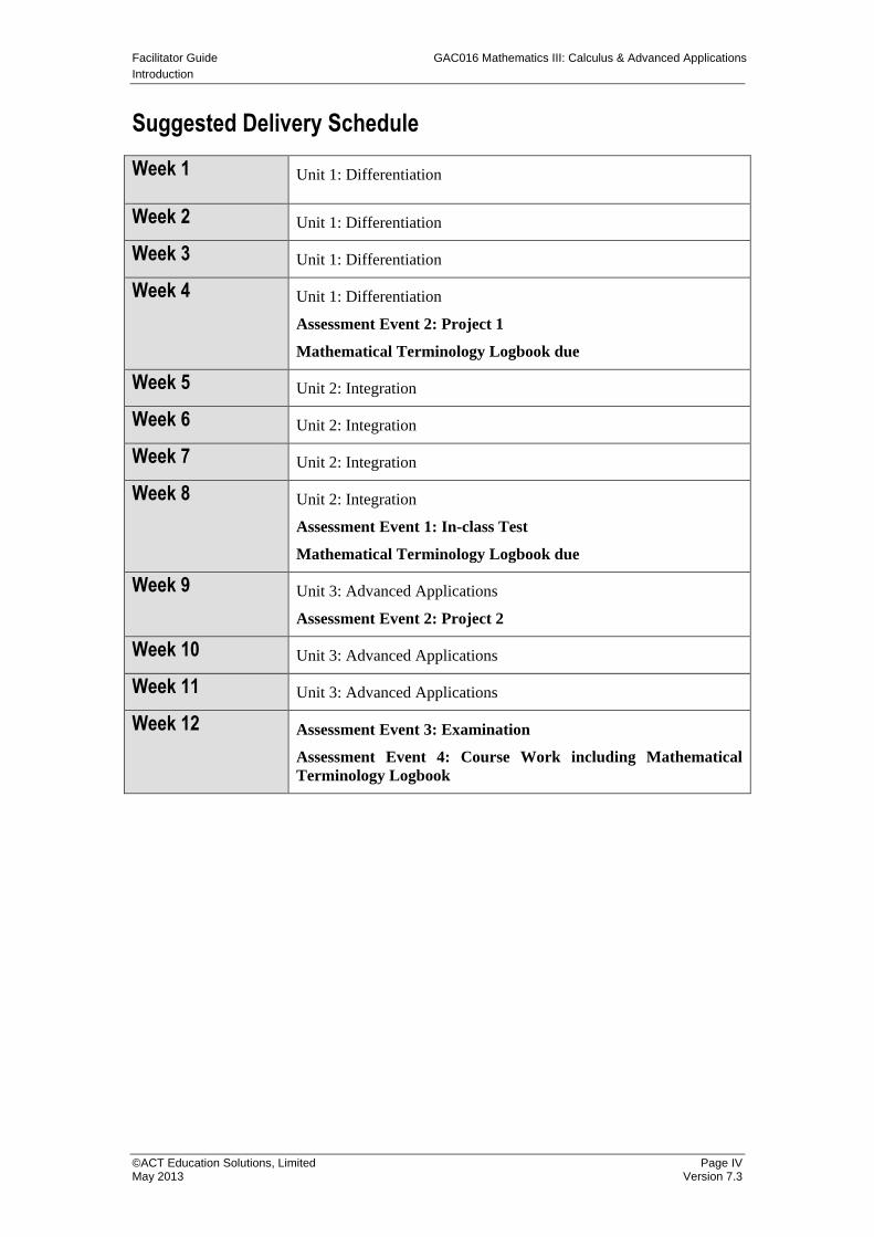
Suggested Delivery Schedule
Week 1
Unit 1: Differentiation
Week 2 Unit 1: Differentiation
Week 3 Unit 1: Differentiation
Week 4 Unit 1: Differentiation
Assessment Event 2: Project 1
Mathematical Terminology Logbook due
Week 5 Unit 2: Integration
Week 6 Unit 2: Integration
Week 7 Unit 2: Integration
Week 8 Unit 2: Integration
Assessment Event 1: In-class Test
Mathematical Terminology Logbook due
Week 9 Unit 3: Advanced Applications
Assessment Event 2: Project 2
Week 10 Unit 3: Advanced Applications
Week 11 Unit 3: Advanced Applications
Week 12 Assessment Event 3: Examination
Assessment Event 4: Course Work including Mathematical
Terminology Logbook
GAC016 Mathematics III: Calculus & Advanced Applications Facilitator Guide
Introduction
Page V ©ACT Education Solutions, Limited Version 7.3 May 2013
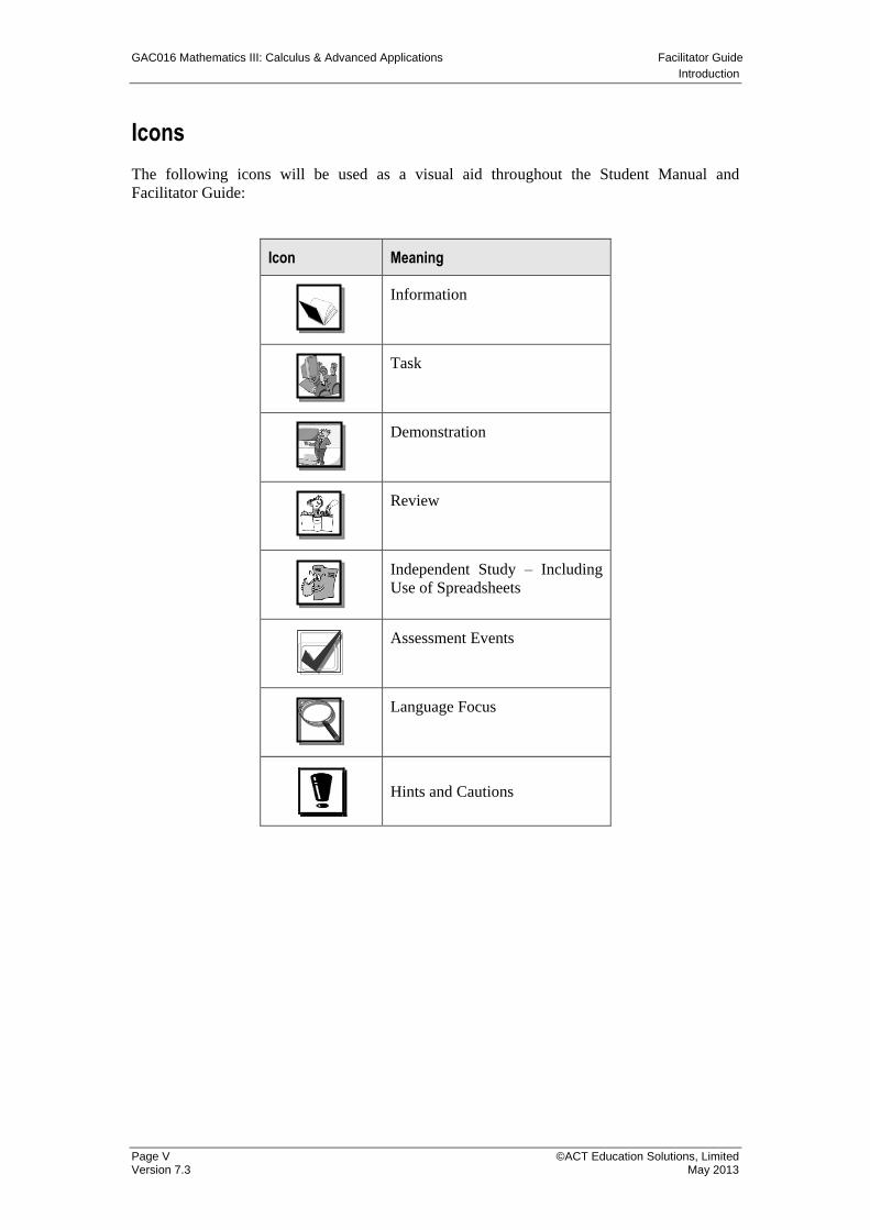
Icons
The following icons will be used as a visual aid throughout the Student Manual and
Facilitator Guide:
Icon Meaning
Information
Task
Demonstration
Review
Independent Study – Including
Use of Spreadsheets
Assessment Events
Language Focus
Hints and Cautions

GAC016 Mathematics III: Calculus & Advanced Applications Facilitator Guide
Unit 1: Differentiation
Page 1 ©ACT Education Solutions, Limited Version 7.3 May 2013
Unit 1: Differentiation
Part A Unit Introduction
Part B Terminology Introduced
Part C Differentiation – Continuity and Limits
Part D The Derivative – Gradients of Secants and Tangents
Part E Differentiation of Functions
Part F Rates of Change
Part G The Product, Quotient and Chain Rules
Part H Differentiation – Exponentials and Logarithms
Part I Applications of the Derivative
Part J Differentiation – Circular Functions
Part K Higher Derivatives
Part L Curve Sketching
Part A Unit Introduction
Overview In this unit, students will learn to apply appropriate methods of
differential calculus to solving various algebraic problems.
In this unit, students will learn to:
differentiate various types of functions from first principles
apply the basic formula for differentiation using the
product, quotient and chain rules where appropriate
find the first and second derivatives
sketch the curve of any function over a given domain.
In Unit 3, the techniques learnt here will be applied to various
problems of quantitative analysis.
This unit includes a series of tasks that students will work through
to practise the course material. They will be expected to complete
some work in their own time. You will guide them through the unit.
Facilitator Guide GAC016 Mathematics III: Calculus & Advanced Applications
Unit 1: Differentiation
©ACT Education Solutions, Limited Page 2 May 2013 Version 7.3
Exploring Calculus
Calculus is about graphs of functions, so this section links very
closely with the sections about graphing functions in GAC004.
There will be many times when ideas from that module are used to
help students understand what is happening in this module. You
should feel free to encourage students to use the spreadsheets about
graphing functions from GAC004.
Assessment Events 1, 2, 3 & 4
Provide students with an overview of the assessment events for this
module. Highlight the timing and nature of projects, the scope of
the review test required for this unit (Test at end of Unit 2), and the
scope and nature of the final examination.
Assessment Event 4
Provide students with an overview of the Mathematical
Terminology Logbook. Students should be familiar with the
requirements of this logbook from previous maths modules. This is
due to be collected at the end of each unit.
GAC016 Mathematics III: Calculus & Advanced Applications Facilitator Guide
Unit 1: Differentiation
Page 3 ©ACT Education Solutions, Limited Version 7.3 May 2013
Part B Terminology Introduced
By the end of this unit, students need to know the meanings of these
terms. The terms are bolded in the first instance they occur. Please
make sure students understand the definitions of new terminology
and include these words in their Mathematical Terminology
Logbook.
Summary of Terms
limit
continuity
derivative
quotient rule
turning point
maximum
absolute maximum
approaches
monotonic point
tangent
differentiation
differentiate
chain rule
stationary point
minimum
absolute minimum
nature
relative maximum
secant
first principles
product rule
second derivative
inflection point
boundary values
normal
extremities
relative minimum
Facilitator Guide GAC016 Mathematics III: Calculus & Advanced Applications
Unit 1: Differentiation
©ACT Education Solutions, Limited Page 4 May 2013 Version 7.3
Part C Differentiation – Continuity and Limits
Exploring Differentiation
Continuity
Limits
Determining Limits
This section is about continuity. This idea is important because of
the idea of the gradient of the tangent to come.
The gradient of the tangent is the limit of the gradient of the
secant (the line joining two points on the curve) as the two points
get closer together. Now if the curve happens to have no values, or
suddenly changes direction, then the limit idea breaks down.
Students refer to spreadsheet Many functions and Student Manual
(pp 4 – 6).
Continuity at a Point
If one or more of the conditions in the definition above fails to be
true, then f(x) is said to be discontinuous at x = a.
Task 1.1
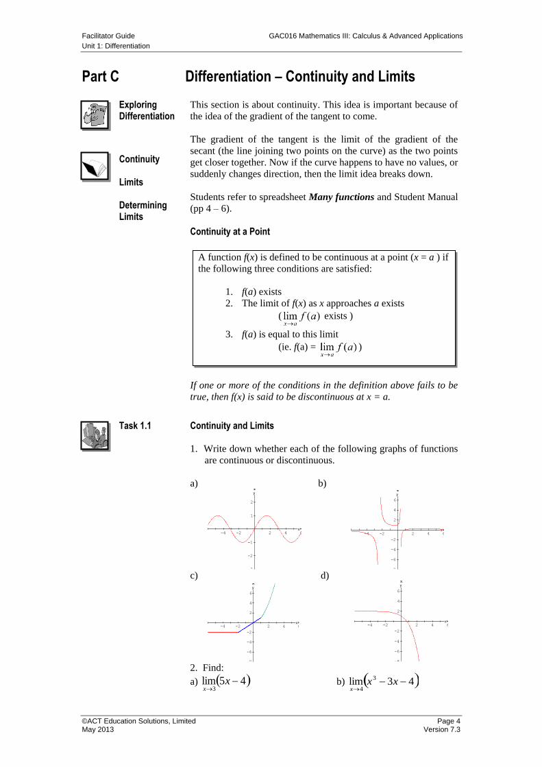
Continuity and Limits 1. Write down whether each of the following graphs of functions
are continuous or discontinuous.
a) b)
c) d)
2. Find:
a) 45lim3
xx
b) 43lim 3
4
xx
x
-4 -2 2 4 6
-3
-2
-1
1
2
x
y
-4 -2 2 4 6
-8
-6
-4
-2
2
4
6
x
y
-4 -2 2 4 6
-8
-6
-4
-2
2
4
6
x
y
-4 -2 2 4 6
-8
-6
-4
-2
2
4
6
x
y
A function f(x) is defined to be continuous at a point (x = a ) if
the following three conditions are satisfied:
1. f(a) exists
2. The limit of f(x) as x approaches a exists
( exists )
3. f(a) is equal to this limit
(ie. f(a) = )
GAC016 Mathematics III: Calculus & Advanced Applications Facilitator Guide
Unit 1: Differentiation
Page 5 ©ACT Education Solutions, Limited Version 7.3 May 2013
c)
xx
x
x 2lim
20 d)
2
6lim
2
2 h
hh
h
e)
3
27lim
3
3 x
x
x f)
m
mmm
m
139lim
23
0
g)
h
hhyyhhy
h
532lim
223
0 h)
6
65lim
2
2
2 aa
aa
a
i)
245
752lim
2
2
tt
tt
t j)
33lim
cx
cx
cx
3. For what values of x is the function
2611
62
xx
xy
discontinuous?
4. Determine whether the function:
f (x)
9
3
1832
x
xx
is continuous at x = 3.
Task 1.1 Solutions
1. a) continuous
b) discontinuous
c) continuous
d) continuous
2. a)
3
limx (5x - 4)
= 5(3) -4 = 11
b) 3
4lim 3 4x
x x
34 3 4 4
48
c)
0
limx
( 2)
x
x x
= 0
limx
1
( 2)x
= 20
1
1
2
x 3
x = 3
Facilitator Guide GAC016 Mathematics III: Calculus & Advanced Applications
Unit 1: Differentiation
©ACT Education Solutions, Limited Page 6 May 2013 Version 7.3
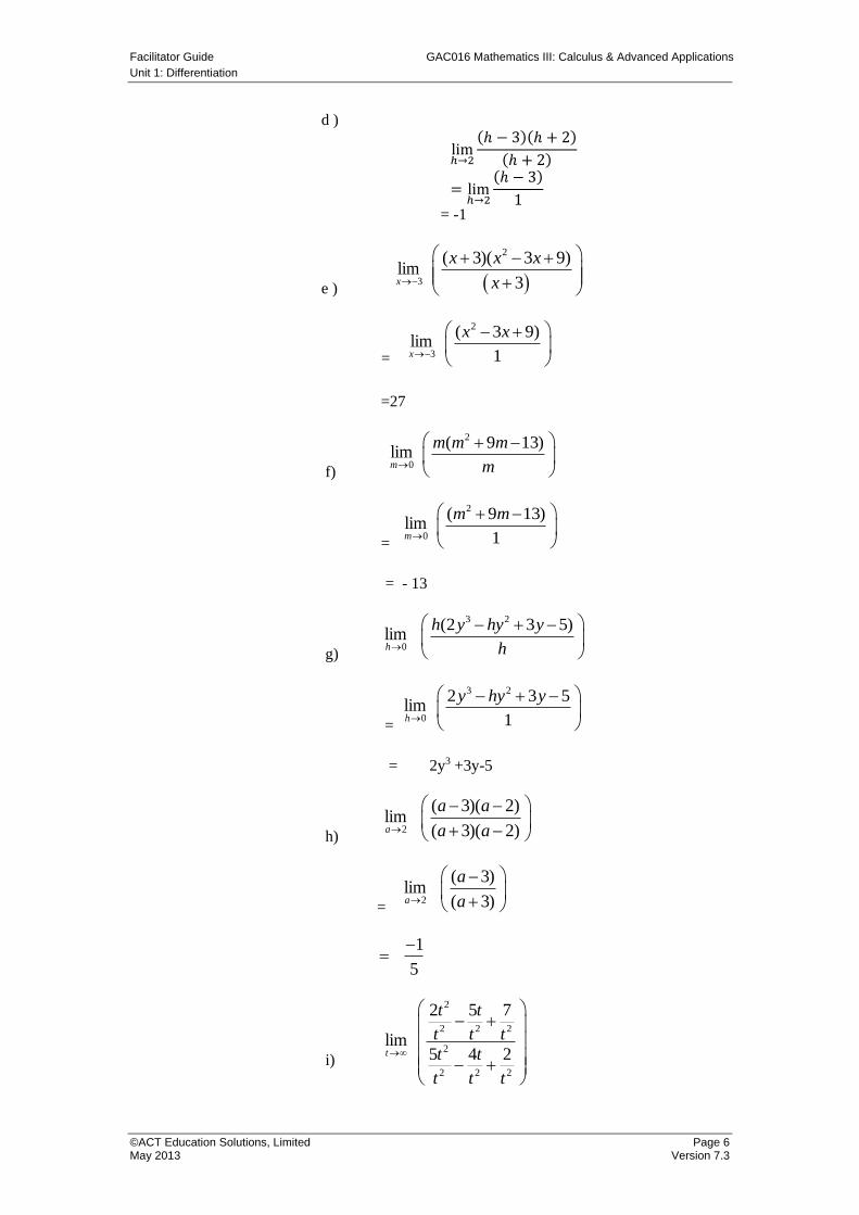
d )
limℎ→2
(ℎ − 3)(ℎ + 2)
(ℎ + 2)
= limℎ→2
(ℎ − 3)
1
= -1
e ) 3
limx
2( 3)( 3 9)
3
x x x
x
= 3
limx
2( 3 9)
1
x x
=27
f)
0
limm
2( 9 13)m m m
m
= 0
limm
2( 9 13)
1
m m
= - 13
g) 0
limh
3 2(2 3 5)h y hy y
h
= 0
limh
3 22 3 5
1
y hy y
= 2y3 +3y-5
h) 2
lima
( 3)( 2)
( 3)( 2)
a a
a a
= 2
lima
( 3)
( 3)
a
a
1
5
i) t
lim
2
2 2 2
2
2 2 2
2 5 7
5 4 2
t t
t t t
t t
t t t
GAC016 Mathematics III: Calculus & Advanced Applications Facilitator Guide
Unit 1: Differentiation
Page 7 ©ACT Education Solutions, Limited Version 7.3 May 2013
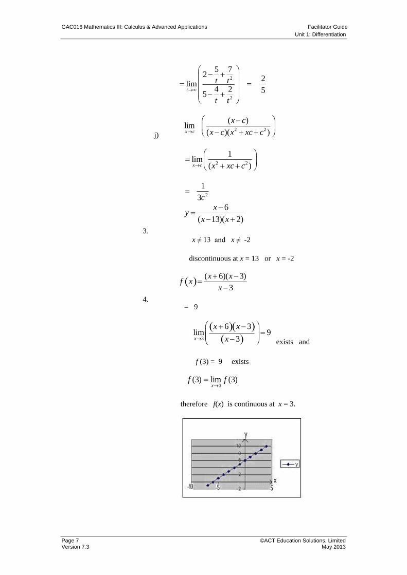
2
2
5 72
lim4 2
5t
t t
t t
2
5
j) cx
lim
2 2
( )
( )( )
x c
x c x xc c
2 2
1lim
( )x c x xc c
2
1
3c
3.
6
( 13)( 2)
xy
x x
x ≠ 13 and x ≠ -2
discontinuous at x = 13 or x = -2
4.
( 6)( 3)
3
x xf x
x
= 9
3
6 3lim 9
3x
x x
x
exists and
f (3) = 9 exists
)3(lim)3(3
ffx
therefore f(x) is continuous at x = 3.
Facilitator Guide GAC016 Mathematics III: Calculus & Advanced Applications
Unit 1: Differentiation
©ACT Education Solutions, Limited Page 8 May 2013 Version 7.3
Part D The Derivative – Gradients of Secants and Tangents
Exploring the Derivative
The Gradient of a Secant
Gradient of a Tangent
The idea of the derivative is the value of the gradient of a curve at a
point. It is the same as the gradient of a tangent to the curve at that
point.
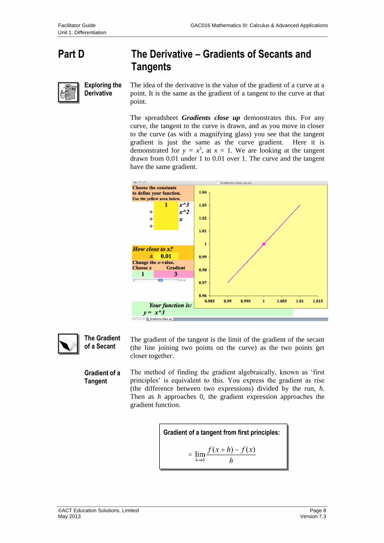
The spreadsheet Gradients close up demonstrates this. For any
curve, the tangent to the curve is drawn, and as you move in closer
to the curve (as with a magnifying glass) you see that the tangent
gradient is just the same as the curve gradient. Here it is
demonstrated for y = x3, at x = 1. We are looking at the tangent
drawn from 0.01 under 1 to 0.01 over 1. The curve and the tangent
have the same gradient.
The gradient of the tangent is the limit of the gradient of the secant
(the line joining two points on the curve) as the two points get
closer together.
The method of finding the gradient algebraically, known as ‘first
principles’ is equivalent to this. You express the gradient as rise
(the difference between two expressions) divided by the run, h.
Then as h approaches 0, the gradient expression approaches the
gradient function.
Gradient of a tangent from first principles:
=
GAC016 Mathematics III: Calculus & Advanced Applications Facilitator Guide
Unit 1: Differentiation
Page 9 ©ACT Education Solutions, Limited Version 7.3 May 2013
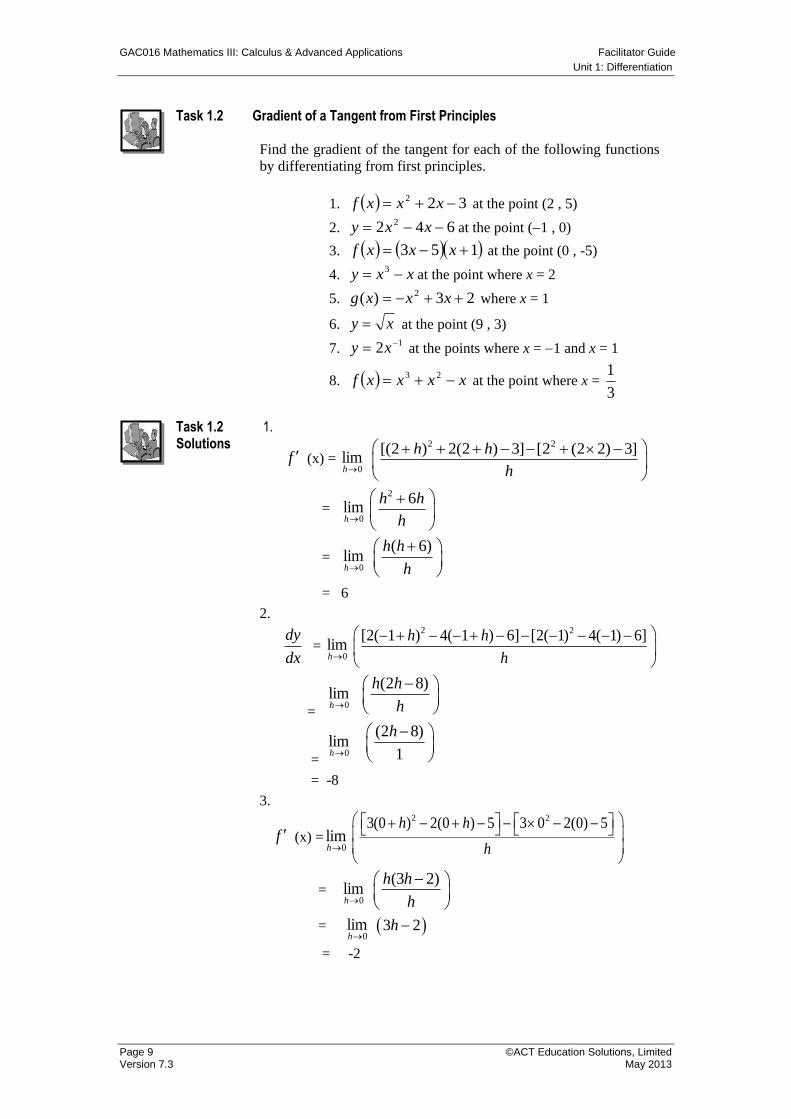
Task 1.2 Gradient of a Tangent from First Principles Find the gradient of the tangent for each of the following functions
by differentiating from first principles.
1. 322 xxxf at the point (2 , 5)
2. 642 2 xxy at the point (1 , 0)
3. 153 xxxf at the point (0 , -5)
4. xxy 3at the point where x = 2
5. 23)( 2 xxxg where x = 1
6. xy at the point (9 , 3)
7. 12 xy at the points where x = 1 and x = 1
8. xxxxf 23 at the point where x =
3
1
Task 1.2 Solutions
1.
f (x) = 0
limh
2 2[(2 ) 2(2 ) 3] [2 (2 2) 3]h h
h
=
0
limh
2 6h h
h
=
0
limh
( 6)h h
h
= 6
2.
dx
dy =
0limh
2 2[2( 1 ) 4( 1 ) 6] [2( 1) 4( 1) 6]h h
h
= 0
limh
(2 8)h h
h
= 0
limh
(2 8)
1
h
= -8
3.
f (x) =0
limh
2 23(0 ) 2(0 ) 5 3 0 2(0) 5h h
h
=
0limh
(3 2)h h
h
=
0limh
3 2h
= -2
Facilitator Guide GAC016 Mathematics III: Calculus & Advanced Applications
Unit 1: Differentiation
©ACT Education Solutions, Limited Page 10 May 2013 Version 7.3
4.
dx
dy =
0
limh
3 3[(2 ) (2 )] [2 2]h h
h
=
0
limh
2(11 6 )h h h
h
=
0
limh
2 6 11h h
= 11
5.
g (x) =
0
limh
2 2[ (1 ) 3(1 ) 2] [ 1 3(1) 2]h h
h
0
limh
( 1)h h
h
0
limh
1 h
= 1
6.
dx
dy =
0limh
1/2 1/2(9 ) 9h
h
0
limh
1/2(9 ) 3h
h
X 1/2
1/2
(9 ) 3
(9 ) 3
h
h
0
limh
( 9 3)
h
h h
0
limh
1
( 9 3)1h
1
9 3
1
6
7.
dx
dy =
0
limh
2 2
x h x
= 0
limh
2
( )
h
x x h
= 0
limh
2
x x
at x = 1 , 2
21 1
dy
dx
at x = 1, 2
21 1
dy
dx
GAC016 Mathematics III: Calculus & Advanced Applications Facilitator Guide
Unit 1: Differentiation
Page 11 ©ACT Education Solutions, Limited Version 7.3 May 2013
8.
dx
dy=
0limh
3 2 3 21 1 1 1 1 1[( ) ( ) ( )] [( ) ( ) ]
3 3 3 3 3 3h h h
h
= 0
limh
2 32h h
h
= 0
limh
22
1
h h
= 0
Facilitator Guide GAC016 Mathematics III: Calculus & Advanced Applications
Unit 1: Differentiation
©ACT Education Solutions, Limited Page 12 May 2013 Version 7.3
Part E Differentiation of Functions
Exploring Differentiation of Functions
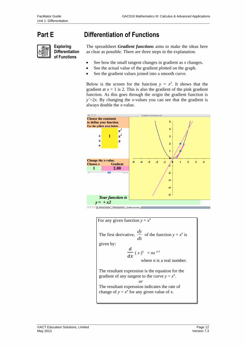
The spreadsheet Gradient functions aims to make the ideas here
as clear as possible. There are three steps in the explanation.
See how the small tangent changes in gradient as x changes.
See the actual value of the gradient plotted on the graph.
See the gradient values joined into a smooth curve.
Below is the screen for the function y = x2. It shows that the
gradient at x = 1 is 2. This is also the gradient of the pink gradient
function. As this goes through the origin the gradient function is
y´=2x. By changing the x-values you can see that the gradient is
always double the x-value.
For any given function y = xn
The first derivative, of the function y = xn is
given by:
𝑑
𝑑𝑥 ( x )n = nx n-1
where n is a real number.
The resultant expression is the equation for the
gradient of any tangent to the curve y = xn.
or
The resultant expression indicates the rate of
change of y = xn for any given value of x.
GAC016 Mathematics III: Calculus & Advanced Applications Facilitator Guide
Unit 1: Differentiation
Page 13 ©ACT Education Solutions, Limited Version 7.3 May 2013
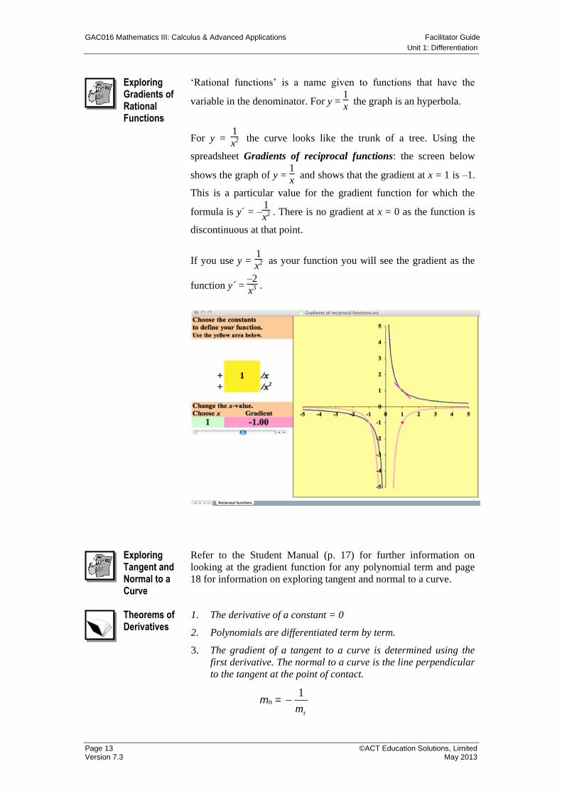
Exploring Gradients of Rational Functions
‘Rational functions’ is a name given to functions that have the
variable in the denominator. For y = 1
x the graph is an hyperbola.
For y = 1
x2 the curve looks like the trunk of a tree. Using the
spreadsheet Gradients of reciprocal functions: the screen below
shows the graph of y = 1
x and shows that the gradient at x = 1 is –1.
This is a particular value for the gradient function for which the
formula is y´ = –1
x2 . There is no gradient at x = 0 as the function is
discontinuous at that point.
If you use y = 1
x2 as your function you will see the gradient as the
function y´ = –2
x3 .
Exploring Tangent and Normal to a Curve
Refer to the Student Manual (p. 17) for further information on
looking at the gradient function for any polynomial term and page
18 for information on exploring tangent and normal to a curve.
Theorems of Derivatives
1. The derivative of a constant = 0
2. Polynomials are differentiated term by term.
3. The gradient of a tangent to a curve is determined using the
first derivative. The normal to a curve is the line perpendicular
to the tangent at the point of contact.
mn = tm
1
Facilitator Guide GAC016 Mathematics III: Calculus & Advanced Applications
Unit 1: Differentiation
©ACT Education Solutions, Limited Page 14 May 2013 Version 7.3
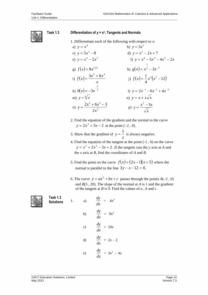
Task 1.3 Differentiation of y = xn, Tangents and Normals
1. Differentiate each of the following with respect to x:
a) 4xy b)
33xy
c) 85 2 xy d) 722 xxy
e) 23 2xxy f) xxxxy 245 346
g) 2518 xxf h) 22
1
3 xxxg
i) x
xxxf
32 63 j) 12
4
1 24 xxxf
k) 3
5
3
xxh l) 321 462 xxxy
m) 6 xy n) xxxy
o) 2
25
2
362
x
xxy
p)
x
xxy
32
2. Find the equation of the gradient and the normal to the curve
232 2 xxy at the point (2 , 0).
3. Show that the gradient of x
y5
is always negative.
4. Find the equation of the tangent at the point (-1 , 6) on the curve
232 23 xxxy . If the tangent cuts the y axis at A and
the x axis at B, find the coordinates of A and B.
5. Find the point on the curve 512 xxxf where the
normal is parallel to the line .0123 xy
6. The curve cbxaxy 2 passes through the points A(2 , 0)
and B(3 , 20). The slope of the normal at A is 1 and the gradient
of the tangent at B is 9. Find the values of a , b and c .
Task 1.3 Solutions
1. a) dx
dy = 4x3
b) dx
dy = 9x2
c) dx
dy = 10x
d) dx
dy = 2x – 2
e) dx
dy = 3x2 - 4x
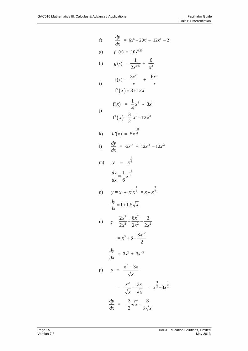
GAC016 Mathematics III: Calculus & Advanced Applications Facilitator Guide
Unit 1: Differentiation
Page 15 ©ACT Education Solutions, Limited Version 7.3 May 2013
f) dx
dy = 6x5 – 20x3 – 12x2 – 2
g) f ' (x) = 10x0.25
h) g'(x) = 5.02
1
x +
3
6
x
i)
2 33 6f(x) = +
f 3 12
x x
x x
x x
j)
6 4
5 3
1f( ) = - 3
4
3f = 12
2
x x x
x x x
k)
8
3'( ) 5 h x x
l) dx
dy = -2x-2 + 12x-3 – 12x-4
m)
1
6 y x
5
61
6
dyx
dx
n)
1 3
1 2 2 = = y x x x x x
1 1.5dy
xdx
o) y
5 2
2 2 2
2 6 3
2 2 2
x x
x x x
23 3
32
xx
dx
dy = 3x2 + 3x -3
p) y = x
xx 32
= x
x
x
x 32
= x 2
1
2
3
3x
dx
dy =
xx
2
3
2
3
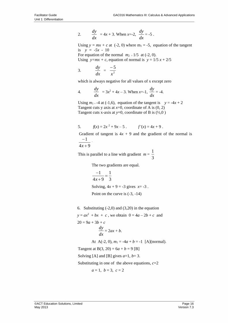
Facilitator Guide GAC016 Mathematics III: Calculus & Advanced Applications
Unit 1: Differentiation
©ACT Education Solutions, Limited Page 16 May 2013 Version 7.3
2. dx
dy = 4x + 3. When x=-2,
dy
dx= -5 .
Using y = mx + c at (-2, 0) where m1 = -5, equation of the tangent
is y = -5x - 10
For equation of the normal m2 = 1/5 at (-2, 0).
Using y=mx + c, equation of normal is y = 1/5 x + 2/5
3. dx
dy =
2
5
x
which is always negative for all values of x except zero
4. dx
dy = 3x2 + 4x – 3. When x=-1,
dy
dx= -4.
Using m1 = -4 at (-1,6), equation of the tangent is y = -4x + 2
Tangent cuts y axis at x=0, coordinate of A is (0, 2)
Tangent cuts x-axis at y=0, coordinate of B is (½,0 )
5. f(x) = 2x 2 + 9x – 5 . f '(x) = 4x + 9 .
Gradient of tangent is 4x + 9 and the gradient of the normal is
94
1
x
.
This is parallel to a line with gradient m = 1
3
The two gradients are equal.
1 1
4 9 3x
Solving, 4x + 9 = -3 gives x= -3 .
Point on the curve is (-3, -14)
6. Substituting (-2,0) and (3,20) in the equation
y = ax2 + bx + c , we obtain 0 = 4a – 2b + c and
20 = 9a + 3b + c
dx
dy= 2ax + b.
At A(-2, 0), m1 = -4a + b = -1 [A](normal).
Tangent at B(3, 20) = 6a + b = 9 [B]
Solving [A] and [B] gives a=1, b= 3.
Substituting in one of the above equations, c=2
a = 1, b = 3, c = 2
GAC016 Mathematics III: Calculus & Advanced Applications Facilitator Guide
Unit 1: Differentiation
Page 17 ©ACT Education Solutions, Limited Version 7.3 May 2013
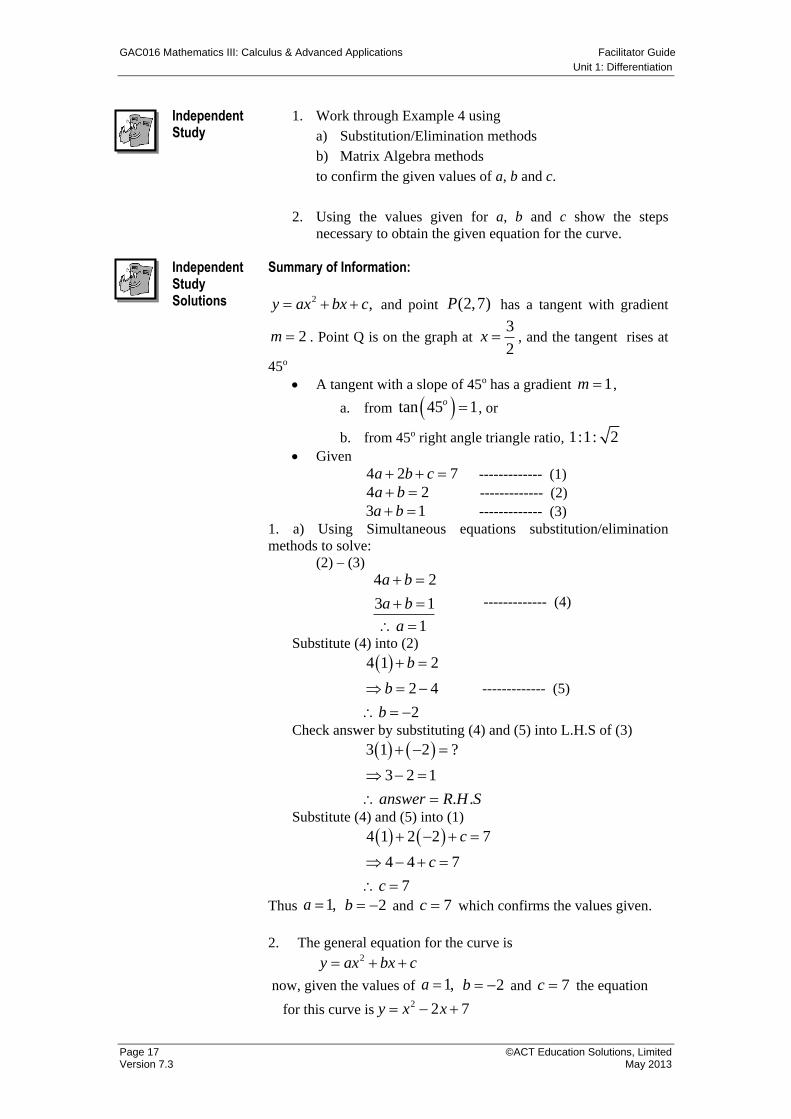
Independent Study
1. Work through Example 4 using
a) Substitution/Elimination methods
b) Matrix Algebra methods
to confirm the given values of a, b and c.
2. Using the values given for a, b and c show the steps
necessary to obtain the given equation for the curve.
Independent Study Solutions
Summary of Information:
2 ,y ax bx c and point (2,7)P has a tangent with gradient
2m . Point Q is on the graph at 3
2x , and the tangent rises at
45o
A tangent with a slope of 45o has a gradient 1m ,
a. from tan 45 1o , or
b. from 45o right angle triangle ratio, 1:1: 2
Given
4 2 7a b c ------------- (1)
4 2a b ------------- (2)
3 1a b ------------- (3)
1. a) Using Simultaneous equations substitution/elimination
methods to solve:
(2) – (3)
4 2
3 1
1
a b
a b
a
------------- (4)
Substitute (4) into (2)
4 1 2
2 4
2
b
b
b
------------- (5)
Check answer by substituting (4) and (5) into L.H.S of (3)
3 1 2 ?
3 2 1
. .answer R H S
Substitute (4) and (5) into (1)
4 1 2 2 7
4 4 7
7
c
c
c
Thus 1,a 2b and 7c which confirms the values given.
2. The general equation for the curve is 2y ax bx c
now, given the values of 1,a 2b and 7c the equation
for this curve is2 2 7y x x
Facilitator Guide GAC016 Mathematics III: Calculus & Advanced Applications
Unit 1: Differentiation
©ACT Education Solutions, Limited Page 18 May 2013 Version 7.3
Part F Rates of Change
Exploring Rates of Change
Distance & Speed
Rates of Change
Rate of Change and Gradients
Rate of Change and Derivatives
It is very useful to relate all this material with abstract functions to
something real that is also understood intuitively by your students.
Motion is a good example of this. At a later point this will extend to
uniformly accelerated motion, but at this stage we will just see that
for any linear distance function the gradient is the speed. The reason
for using the complex spreadsheet at this stage is to prepare students
for the more complex situations later.
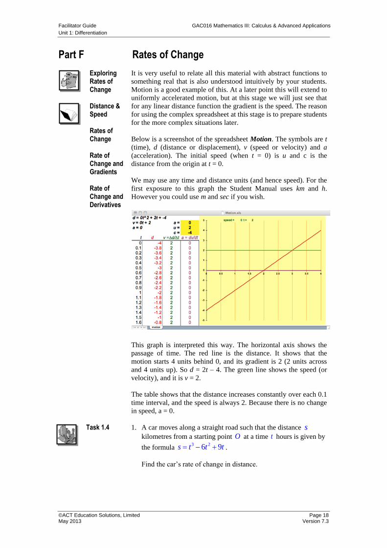
Below is a screenshot of the spreadsheet Motion. The symbols are t
(time), d (distance or displacement), v (speed or velocity) and a
(acceleration). The initial speed (when t = 0) is u and c is the
distance from the origin at t = 0.
We may use any time and distance units (and hence speed). For the
first exposure to this graph the Student Manual uses km and h.
However you could use m and sec if you wish.
This graph is interpreted this way. The horizontal axis shows the
passage of time. The red line is the distance. It shows that the
motion starts 4 units behind 0, and its gradient is 2 (2 units across
and 4 units up). So d = 2t – 4. The green line shows the speed (or
velocity), and it is v = 2.
The table shows that the distance increases constantly over each 0.1
time interval, and the speed is always 2. Because there is no change
in speed, a = 0.
Task 1.4 1. A car moves along a straight road such that the distance s
kilometres from a starting point O at a time t hours is given by
the formula 3 26 9s t t t .
Find the car’s rate of change in distance.
GAC016 Mathematics III: Calculus & Advanced Applications Facilitator Guide
Unit 1: Differentiation
Page 19 ©ACT Education Solutions, Limited Version 7.3 May 2013
2. If the cost of supply of raw fish to a fish monger is
250 40 0.01C f f , calculate the rate of change of cost of
supplying 48 tonnes of fish.
Solutions Task 1.4
1. Let 3 2( ) 6 9f t S t t t
Rate of change ,ds
dt or '( )f S
Using 1n ndx nx
dx
Then,
3 2
6 9d
t t tdt
3 1 2 1 1 13 6 2 9t t t
23 12 9t t
rate of change in distance is given by 23 12 9t t
2. Let 250 40 0.01 ;C f f 48f tonnes.
Cost 250 40 0.01dC d
f fdf df
40 0.02 f
When 48f ; rate of change of cost 40 0.02 48
$39.04
Facilitator Guide GAC016 Mathematics III: Calculus & Advanced Applications
Unit 1: Differentiation
©ACT Education Solutions, Limited Page 20 May 2013 Version 7.3
Part G The Product, Quotient and Chain Rules
Exploring the Product Rule
The Product Rule
The reason we need a product rule is that some functions cannot be
simply expanded. An example would be y = x2 ex. However the best
way to explain and justify the rule is to use examples where we can
actually check that the rule works – products of two polynomial
functions that can be multiplied to form the product function.
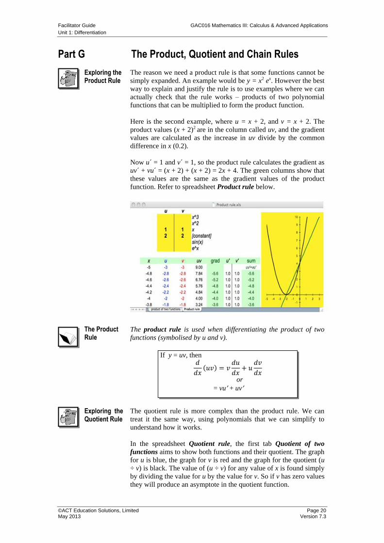
Here is the second example, where u = x + 2, and v = x + 2. The
product values (x + 2)2 are in the column called uv, and the gradient
values are calculated as the increase in uv divide by the common
difference in x (0.2).
Now u´ = 1 and v´ = 1, so the product rule calculates the gradient as
uv´ + vu´ = (x + 2) + (x + 2) = 2x + 4. The green columns show that
these values are the same as the gradient values of the product
function. Refer to spreadsheet Product rule below.
The product rule is used when differentiating the product of two
functions (symbolised by u and v).
Exploring the Quotient Rule
The quotient rule is more complex than the product rule. We can
treat it the same way, using polynomials that we can simplify to
understand how it works.
In the spreadsheet Quotient rule, the first tab Quotient of two
functions aims to show both functions and their quotient. The graph
for u is blue, the graph for v is red and the graph for the quotient (u
÷ v) is black. The value of (u ÷ v) for any value of x is found simply
by dividing the value for u by the value for v. So if v has zero values
they will produce an asymptote in the quotient function.
If y = uv, then 𝑑
𝑑𝑥(𝑢𝑣) = 𝑣
𝑑𝑢
𝑑𝑥+ 𝑢
𝑑𝑣
𝑑𝑥
or
= vu + uv
GAC016 Mathematics III: Calculus & Advanced Applications Facilitator Guide
Unit 1: Differentiation
Page 21 ©ACT Education Solutions, Limited Version 7.3 May 2013
The Quotient Rule
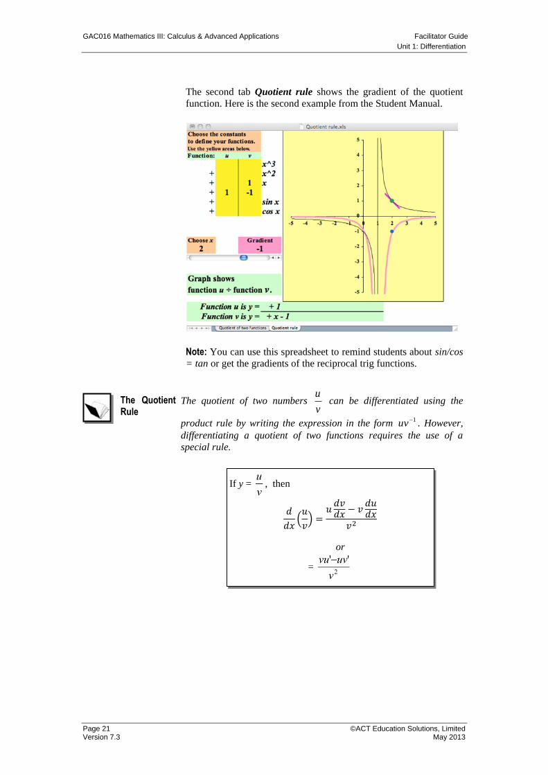
The second tab Quotient rule shows the gradient of the quotient
function. Here is the second example from the Student Manual.
Note: You can use this spreadsheet to remind students about sin/cos
= tan or get the gradients of the reciprocal trig functions.
The quotient of two numbers v
u can be differentiated using the
product rule by writing the expression in the form 1uv . However,
differentiating a quotient of two functions requires the use of a
special rule.
If y = , then
𝑑
𝑑𝑥ቀ
𝑢
𝑣ቁ =
𝑢𝑑𝑣𝑑𝑥
− 𝑣𝑑𝑢𝑑𝑥
𝑣2
or
=
Facilitator Guide GAC016 Mathematics III: Calculus & Advanced Applications
Unit 1: Differentiation
©ACT Education Solutions, Limited Page 22 May 2013 Version 7.3
Exploring The Chain Rule
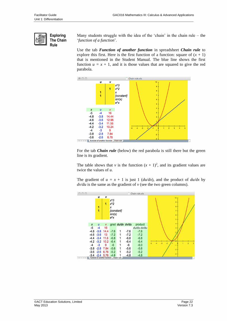
Many students struggle with the idea of the ‘chain’ in the chain rule – the
‘function of a function’.
Use the tab Function of another function in spreadsheet Chain rule to
explore this first. Here is the first function of a function: square of (x + 1)
that is mentioned in the Student Manual. The blue line shows the first
function u = x + 1, and it is those values that are squared to give the red
parabola.
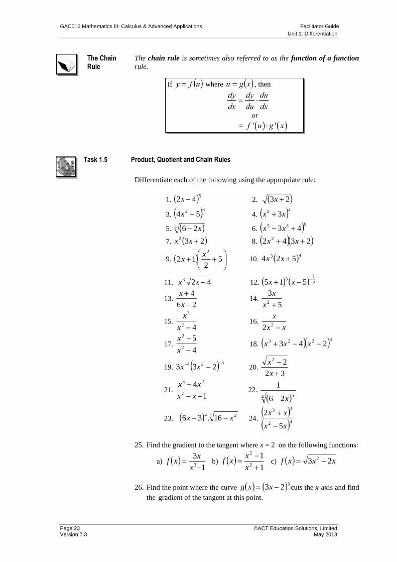
For the tab Chain rule (below) the red parabola is still there but the green
line is its gradient.
The table shows that v is the function (x + 1)2, and its gradient values are
twice the values of u.
The gradient of u = x + 1 is just 1 (du/dx), and the product of du/dx by
dv/du is the same as the gradient of v (see the two green columns).
GAC016 Mathematics III: Calculus & Advanced Applications Facilitator Guide
Unit 1: Differentiation
Page 23 ©ACT Education Solutions, Limited Version 7.3 May 2013
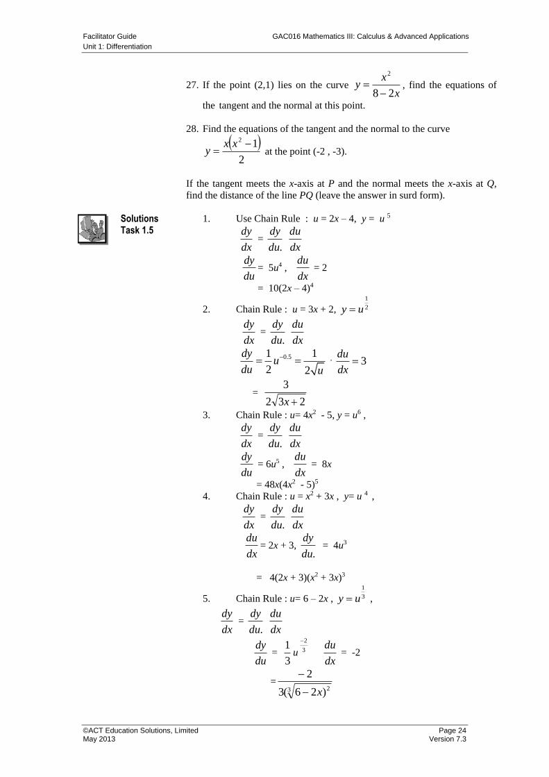
The Chain Rule
The chain rule is sometimes also referred to as the function of a function
rule.
Task 1.5 Product, Quotient and Chain Rules
Differentiate each of the following using the appropriate rule:
1. 542 x 2. 23 x
3. 62 54 x 4. 42 3xx
5. 3 26 x 6. 635 43 xx
7. 232 xx 8. 2342 2 xx
9.
5
212
2xx 10. 43 524 xx
11. 423 xx 12. 2
13
515
xx
13. 26
4
x
x 14.
5
32 x
x
15. 42
3
x
x 16.
xx
x
22
17. 4
52
2
x
x 18. 4223 243 xxx
19. 324 233 xx 20.
32
22
x
x
21. 1
42
23
xx
xx 22.
4 526
1
x
23. 4 2416.36 xx 24.
42
33
5
2
xx
xx
25. Find the gradient to the tangent where x = 2 on the following functions:
a) 1
33
x
xxf b)
1
12
2
x
xxf c) xxxf 23 2
26. Find the point where the curve 323 xxg cuts the x-axis and find
the gradient of the tangent at this point.
If where , then
or
=
Facilitator Guide GAC016 Mathematics III: Calculus & Advanced Applications
Unit 1: Differentiation
©ACT Education Solutions, Limited Page 24 May 2013 Version 7.3
27. If the point (2,1) lies on the curve x
xy
28
2
, find the equations of
the tangent and the normal at this point.
28. Find the equations of the tangent and the normal to the curve
2
12
xxy at the point (-2 , -3).
If the tangent meets the x-axis at P and the normal meets the x-axis at Q,
find the distance of the line PQ (leave the answer in surd form).
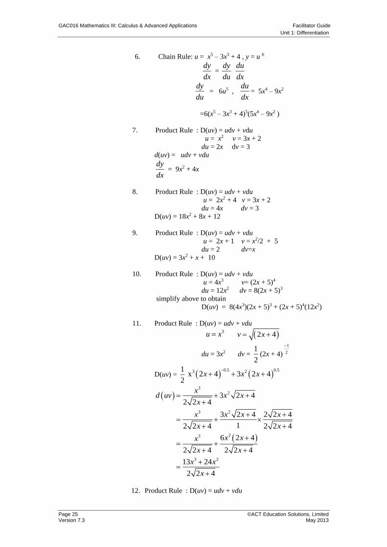
Solutions Task 1.5
1. Use Chain Rule : u = 2x – 4, y = u 5
dx
dy =
.du
dy dx
du
dy
du= 5u4 ,
dx
du = 2
= 10(2x – 4)4
2. Chain Rule : u = 3x + 2,
1
2y u
dx
dy =
.du
dy dx
du
0.51 1
2 2
dyu
du u
, 3du
dx
= 232
3
x
3. Chain Rule : u= 4x2 - 5, y = u6 ,
dx
dy =
.du
dy dx
du
dy
du = 6u5 ,
dx
du = 8x
= 48x(4x2 - 5)5
4. Chain Rule : u = x2 + 3x , y= u 4 ,
dx
dy =
.du
dy dx
du
dx
du= 2x + 3,
.du
dy = 4u3
= 4(2x + 3)(x2 + 3x)3
5. Chain Rule : u= 6 – 2x ,
1
3y u ,
dx
dy =
.du
dy dx
du
dy
du =
1
3u 3
2
dx
du = -2
=3 2)26(3
2
x
GAC016 Mathematics III: Calculus & Advanced Applications Facilitator Guide
Unit 1: Differentiation
Page 25 ©ACT Education Solutions, Limited Version 7.3 May 2013
6. Chain Rule: u = x5 – 3x3 + 4 , y = u 6
dx
dy =
dy
du dx
du
dy
du = 6u5 ,
dx
du= 5x4 – 9x2
=6(x5 – 3x3 + 4)5(5x4 – 9x2 )
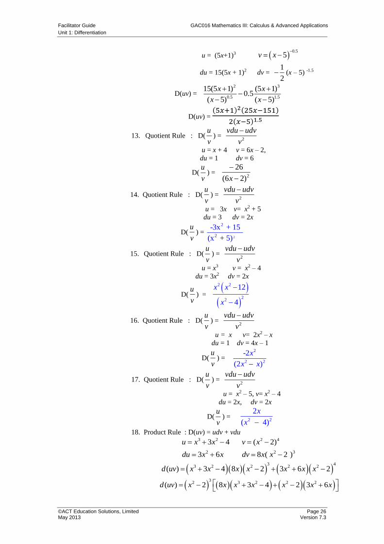
7. Product Rule : D(uv) = udv + vdu
u = x2 v = 3x + 2
du = 2x dv = 3
d(uv) = udv + vdu
dx
dy = 9x2 + 4x
8. Product Rule : D(uv) = udv + vdu
u = 2x2 + 4 v = 3x + 2
du = 4x dv = 3
D(uv) = 18x2 + 8x + 12
9. Product Rule : D(uv) = udv + vdu
u = 2x + 1 v = x2/2 + 5
du = 2 dv=x
D(uv) = 3x2 + x + 10
10. Product Rule : D(uv) = udv + vdu
u = 4x3 v= (2x + 5)4
du = 12x2 dv = 8(2x + 5)3
simplify above to obtain
D(uv) = 8(4x3)(2x + 5)3 + (2x + 5)4(12x2)
11. Product Rule : D(uv) = udv + vdu
3u x 2 4v x
du = 3x2 dv = 1
2(2x + 4) 2
1
D(uv) = 1
2
0.5 0.53 2x 2 4 3 2 4x x x
32
3 2
23
3 2
3 2 42 2 4
3 2 4 2 2 4
12 2 4 2 2 4
6 2 4
2 2 4 2 2 4
13 24
2 2 4
xd uv x x
x
x x x x
x x
x xx
x x
x x
x
12. Product Rule : D(uv) = udv + vdu
Facilitator Guide GAC016 Mathematics III: Calculus & Advanced Applications
Unit 1: Differentiation
©ACT Education Solutions, Limited Page 26 May 2013 Version 7.3
u = (5x+1)3 0.5
5v x
du = 15(5x + 1)2 dv = 1
2 (x – 5) -1.5
D(uv) =
2 3
0.5 1.5
15(5 1) (5 1)0.5
( 5) ( 5)
x x
x x
D(uv) = (5𝑥+1)2(25𝑥−151)
2(𝑥−5)1.5
13. Quotient Rule : D(v
u) =
2v
udvvdu
u = x + 4 v = 6x – 2,
du = 1 dv = 6
D(v
u) =
2)26(
26
x
14. Quotient Rule : D(v
u) =
2v
udvvdu
u = 3x v= x2 + 5
du = 3 dv = 2x
D(v
u) =
2
2
2
-3x + 15
(x + 5)
15. Quotient Rule : D(v
u) =
2v
udvvdu
u = x3 v = x2 – 4
du = 3x2 dv = 2x
D(v
u) =
2 2
22
12
4
x x
x
16. Quotient Rule : D(v
u) =
2v
udvvdu
u = x v= 2x2 – x
du = 1 dv = 4x – 1
D(v
u) =
2
2 2
-2
(2 )
x
x x
17. Quotient Rule : D(v
u) =
2v
udvvdu
u = x2 – 5, v= x2 – 4
du = 2x, dv = 2x
D(v
u) =
2 2
2
( 4)
x
x
18. Product Rule : D(uv) = udv + vdu
3 2 2 4
2 2 3
3 4 ( 2)
3 6 8 ( 2 )
u x x v x
du x x dv x x
3 4
3 2 2 2 2( ) 3 4 8 2 3 6 2d uv x x x x x x x
3
2 3 2 2 2( ) 2 8 3 4 2 3 6d uv x x x x x x x
GAC016 Mathematics III: Calculus & Advanced Applications Facilitator Guide
Unit 1: Differentiation
Page 27 ©ACT Education Solutions, Limited Version 7.3 May 2013
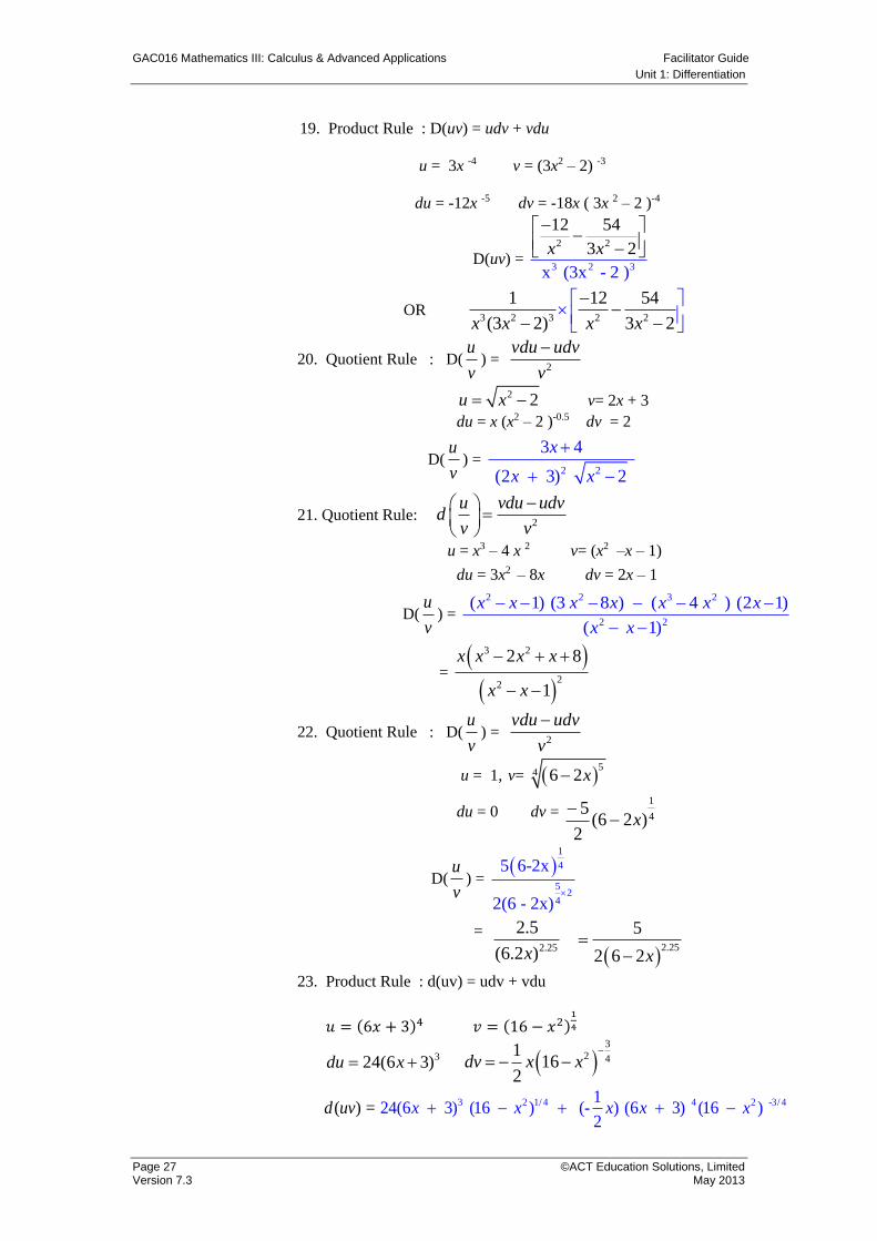
19. Product Rule : D(uv) = udv + vdu
u = 3x -4 v = (3x2 – 2) -3
du = -12x -5 dv = -18x ( 3x 2 – 2 )-4
D(uv) = 3 2 3
2 2
12 54
3 2
x (3x - 2 )
x x
OR 3 2 3 2 2
1 12 54
(3 2) 3 2x x x x
20. Quotient Rule : D(v
u) =
2v
udvvdu
2 2u x v= 2x + 3
du = x (x2 – 2 )-0.5 dv = 2
D(v
u) =
2 2
3 4
(2 3) 2
x
x x
21. Quotient Rule: 2
u vdu udvd
v v
u = x3 – 4 x 2 v= (x2 –x – 1)
du = 3x2 – 8x dv = 2x – 1
D(v
u) =
2 2 3 2
2 2
( 1) (3 8 ) ( 4 ) (2 1)
( 1)
x x x x x x x
x x
=
3 2
22
2 8
1
x x x x
x x
22. Quotient Rule : D(v
u) =
2v
udvvdu
u = 1, v= 5
4 6 2x
du = 0 dv = 4
1
)26(2
5x
D(
v
u) =
1
4
52
4
5 6-2x
2(6 - 2x)
= 25.2)2.6(
5.2
x
2.25
5
2 6 2x
23. Product Rule : d(uv) = udv + vdu
𝑢 = (6𝑥 + 3)4 𝑣 = (16 − 𝑥2)1
4
324(6 3)du x
32 4
116
2dv x x
3 2 1/ 4 4 2 -3/ 41
24(6 3) (16 ) (- ) (6 3)( ) (16 )= 2
x x x xv xd u
Facilitator Guide GAC016 Mathematics III: Calculus & Advanced Applications
Unit 1: Differentiation
©ACT Education Solutions, Limited Page 28 May 2013 Version 7.3
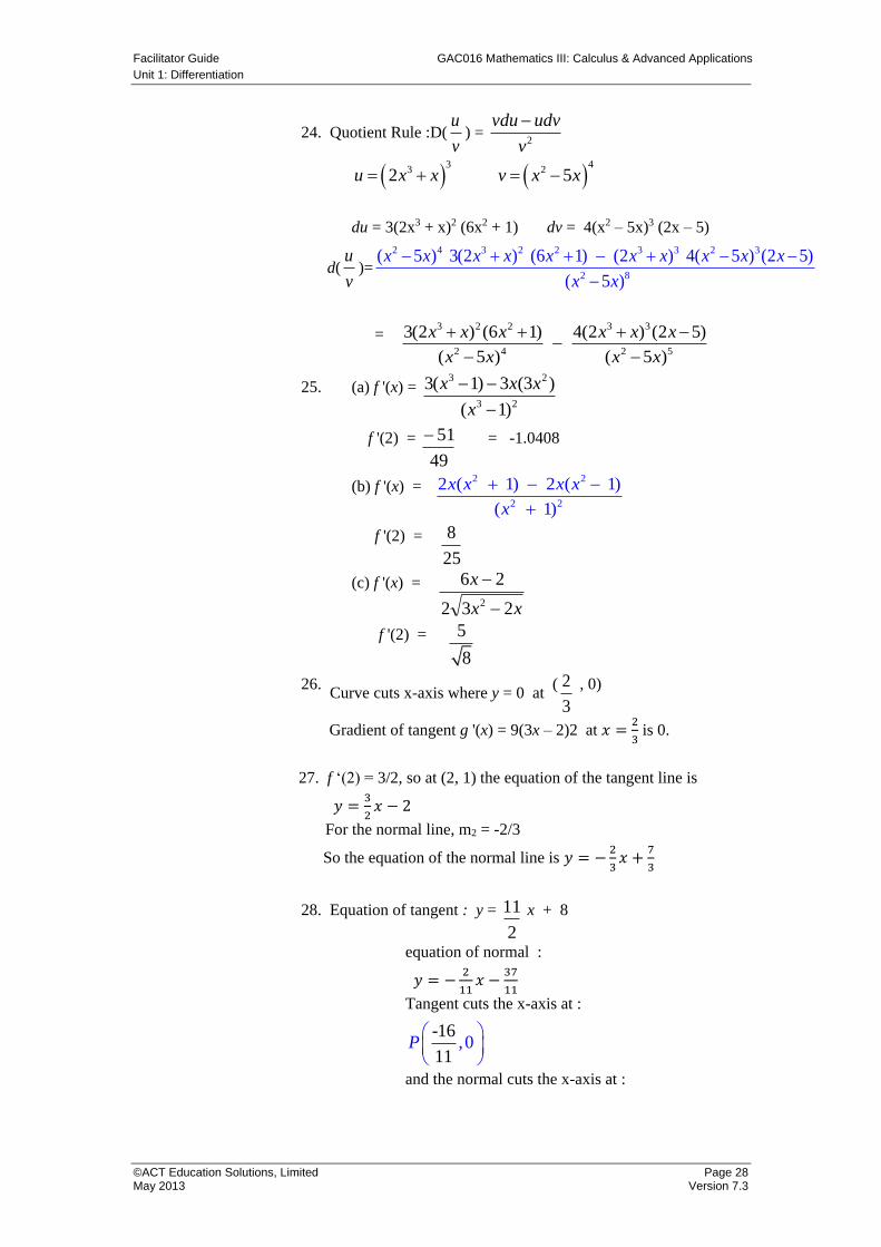
24. Quotient Rule :D(v
u) =
2v
udvvdu
3 4
3 22 5u x x v x x
du = 3(2x3 + x)2 (6x2 + 1) dv = 4(x2 – 5x)3 (2x – 5)
d(v
u)=
2 4 3 2 2 3 3 2 3
2 8
( 5 ) 3(2 ) (6 1) (2 ) 4( 5 ) (2 5)
( 5 )
x x x x x x x x x x
x x
= 3 2 2 3 3
2 4 2 5
3(2 ) (6 1) 4(2 ) (2 5)
( 5 ) ( 5 )
x x x x x x
x x x x
25. (a) f '(x) = 23
23
)1(
)3(3)1(3
x
xxx
f '(2) =
49
51 = -1.0408
(b) f '(x) = 2 2
2 2
2 ( 1) 2 ( 1)
( 1)
x x x x
x
f '(2) =
25
8
(c) f '(x) =
xx
x
232
26
2
f '(2) = 5
8
26. Curve cuts x-axis where y = 0 at
( 2
3
, 0)
Gradient of tangent
g '(x) = 9(3x – 2)2 at 𝑥 =
2
3 is 0.
27. f ‘(2) = 3/2, so at (2, 1) the equation of the tangent line is
𝑦 =3
2𝑥 − 2
For the normal line, m2 = -2/3
So the equation of the normal line is 𝑦 = −2
3𝑥 +
7
3
28. Equation of tangent : y =
2
11 x + 8
equation of normal :
𝑦 = −
2
11𝑥 −
37
11
Tangent cuts the x-axis at :
,0-16
11P
and the normal cuts the x-axis at :
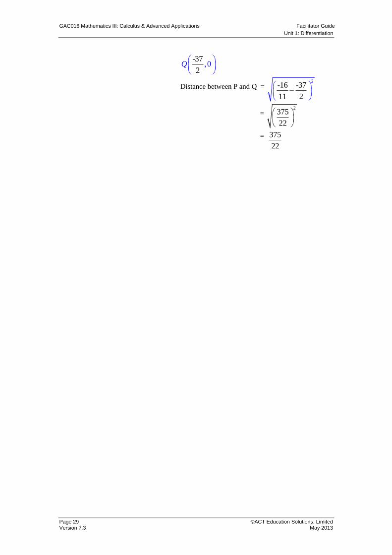
GAC016 Mathematics III: Calculus & Advanced Applications Facilitator Guide
Unit 1: Differentiation
Page 29 ©ACT Education Solutions, Limited Version 7.3 May 2013
,0-37
2Q
Distance between P and Q = 2
-16 -37
11 2
= 2
375
22
= 375
22
Facilitator Guide GAC016 Mathematics III: Calculus & Advanced Applications
Unit 1: Differentiation
©ACT Education Solutions, Limited Page 30 May 2013 Version 7.3
Part H Differentiation – Exponentials and Logarithms
Exploring Differentiation of Exponential Functions
Differentiation of Exponential Functions
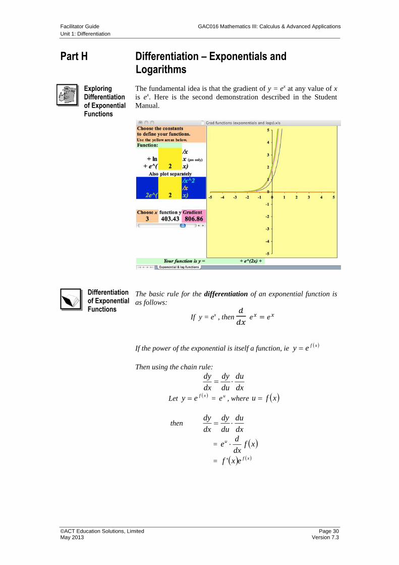
The fundamental idea is that the gradient of y = ex at any value of x
is ex. Here is the second demonstration described in the Student
Manual.
The basic rule for the differentiation of an exponential function is
as follows:
If y = ex , then 𝑑
𝑑𝑥 𝑒𝑥 = 𝑒𝑥
If the power of the exponential is itself a function, ie xfey
Then using the chain rule:
dx
du
du
dy
dx
dy
Let xfey =
ue , where xfu
then dx
du
du
dy
dx
dy
= xfdx
deu
= xfexf '
GAC016 Mathematics III: Calculus & Advanced Applications Facilitator Guide
Unit 1: Differentiation
Page 31 ©ACT Education Solutions, Limited Version 7.3 May 2013
Therefore, the rules of differentiation for exponential functions are:
Differentiation of Logarithmic Functions
Exploring Differentiation of Logarithmic Functions
From Student Manual (pages 31 – 32)
Therefore the rules for differentiation of logarithms are:
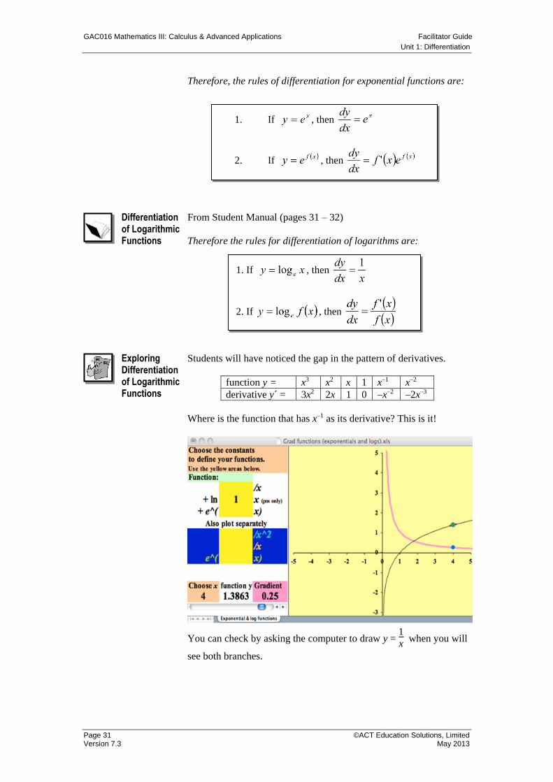
Students will have noticed the gap in the pattern of derivatives.
function y = x3 x2 x 1 x–1 x–2
derivative y´ = 3x2 2x 1 0 –x–2 –2x–3
Where is the function that has x–1 as its derivative? This is it!
You can check by asking the computer to draw y = 1
x when you will
see both branches.
1. If , then
2. If , then
1. If , then
2. If , then
Facilitator Guide GAC016 Mathematics III: Calculus & Advanced Applications
Unit 1: Differentiation
©ACT Education Solutions, Limited Page 32 May 2013 Version 7.3
Two Special Results
From Student Manual, pages 33 – 34.
1. The Derivative of y = ax
If xay
x
ee ay loglog
axy lnln
a
yx
ln
ln
yady
dx 1
ln
1
aydx
dyln
= aa x ln
2. The Derivative of y = logax
If xy alog
Using the change of base law, a
xy
e
e
log
log
xadx
dy
e
1
log
1
Task 1.6
Differentiation of Exponentials and Logarithms
Differentiate each of the following:
1. xey 4 2.
xey
2
1
3. 13 2 xey 4.
xey 27
5. 2
32 xexy 6. 2
3
9 x
ey
x
7. 13log xy e 8. 221ln xy
9. 3log xxy e 10. 4ln 3 xey
11.
2
ln2
xy x 12.
4
3log
2x
xy e
If , then
If , then
GAC016 Mathematics III: Calculus & Advanced Applications Facilitator Guide
Unit 1: Differentiation
Page 33 ©ACT Education Solutions, Limited Version 7.3 May 2013
13. Find the gradients of the tangent and the normal to the curve
xey 32 at the point x = 2.
14. Find the equations of the tangent and the normal to the curve
3log xxf e at the point where x = 1.
15. Find the equations of the tangents to the curve xey 2 where
x = 2 and x = 2. Hence, find the point T where the two tangents
intersect each other.
Solutions Task 1.6
1. Chain Rule : u= 4x , y = eu ;
du
dy =
ue , dx
du = 4
dx
dy =
du
dy
dx
du
= 4e4x
2. Quotient Rule : u = 1, v = e2x ,
dv = 2e 2x , du = 0
D2v
udvvdu
v
u
dx
dy = -2e-2x
3. Chain Rule : u = 3x2 – 1, y = eu ,
dx
dy =
du
dy
dx
du
du
dy =
ue , dx
du= 6x
23 16 xdy
xedx
Facilitator Guide GAC016 Mathematics III: Calculus & Advanced Applications
Unit 1: Differentiation
©ACT Education Solutions, Limited Page 34 May 2013 Version 7.3
4. Chain Rule : u= 7 – 2x, y = eu ,
dx
dy =
du
dy
dx
du
du
dy = eu ,
dx
du= -2
dx
dy = -2e7 – 2x
5. Product Rule : u = 2x – 3, v = ex2 ,
du = 2, dv = 2xe2x
dx
dy = 2ex
2
(2x2 – 3x + 1)
6. Quotient Rule : u = e3x , v = 9 + x2
D2v
udvvdu
v
u
du = 3e3x , dv = 2x
dx
dy =
3 2
2 2
( 27 3 2 )
(9 )
xe x x
x
7. Chain Rule : u = 3x + 1, y = ln u ;
dx
dy =
du
dy
dx
du
du
dy = 1/u ,
dx
du = 3
dx
dy =
13
3
x
8. Chain Rule : u = 1 – 2x2 , y = ln u ;
dx
dy =
du
dy
dx
du
du
dy = 1/u ,
dx
du= -4x
dx
dy =
221
4
x
x
GAC016 Mathematics III: Calculus & Advanced Applications Facilitator Guide
Unit 1: Differentiation
Page 35 ©ACT Education Solutions, Limited Version 7.3 May 2013
9. Chain Rule : u = x – x3 , y = ln( – u) ,
dx
dy =
du
dy
dx
du
du
dy =
1
u ,
dx
du= 1 – 3x2
dx
dy =
2
3
1 3
-
x
x x
10. Chain Rule : u = e3x + 4, y = ln u ;
dx
dy =
du
dy
dx
du
du
dy = 1/ u,
dx
du =
33 xe
dx
dy =
3
3
3
4
x
x
e
e
11. Product Rule : u =
2
2
x , v = ln x ;
( )u
d udv vduv
du = x, dv = 1/x
dx
dy = ln
2
xx x
12. y = ln (x – 3) – ln (x2 – 4 )
dx
dy =
3
1
x –
4
22 x
x
13. dx
dy = 6e3x .
The gradient of tangent at x=2 is 6e6
Hence the gradient of normal : – 66
1
e = - 0.0004
14. f '(x) = x
3
Gradient of tangent = -3.
Equation of tangent at (-1, 0)
using y = mx + c is y = -3x – 3
Gradient of normal = 1
3.
Equation of normal at (-1, 0) is
1 1
3 3y x
Facilitator Guide GAC016 Mathematics III: Calculus & Advanced Applications
Unit 1: Differentiation
©ACT Education Solutions, Limited Page 36 May 2013 Version 7.3
15. Equation for the gradient of tangent is
dx
dy = e-x
Equation of tangent using y = mx + c at (-2, 2 – e2 ) with m = e2
=7.389 is y = xe2 + e2 + 2
Equation of tangent using y = mx + c at (2, 2 – e-2) with m= e-2 is
y = 2
1
ex –
2
3
e + 2
point of intersection : solve xe2 + e2 + 2
= 2
1
ex –
2
3
e + 2
4
4
3
1
ex
e
,
4
4 2 2
3 1 32
1
ey
e e e
Co-ordinates are ( -1.075, 1.449)
GAC016 Mathematics III: Calculus & Advanced Applications Facilitator Guide
Unit 1: Differentiation
Page 37 ©ACT Education Solutions, Limited Version 7.3 May 2013
Part I Applications of the Derivative
Significance of the First Derivative Stationary Points Maximum Turning Point Exploring Horizontal Point of Inflection
Refer to the Student Manual (pp 35 – 38).
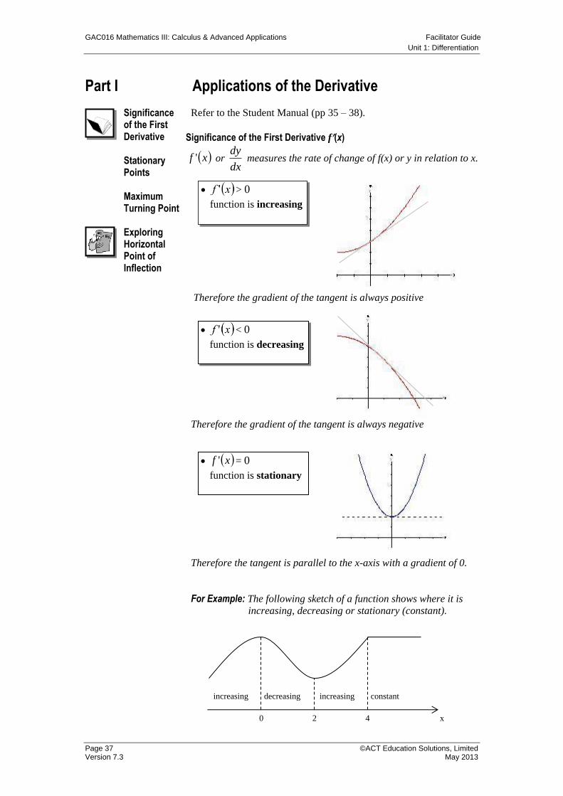
Significance of the First Derivative f(x)
xf ' or dx
dy measures the rate of change of f(x) or y in relation to x.
Therefore the gradient of the tangent is always positive
Therefore the gradient of the tangent is always negative
Therefore the tangent is parallel to the x-axis with a gradient of 0.
For Example: The following sketch of a function shows where it is
increasing, decreasing or stationary (constant).
> 0
function is increasing
< 0
function is decreasing
xf ' = 0
function is stationary
increasing constant increasing decreasing
0 2 4 x
Facilitator Guide GAC016 Mathematics III: Calculus & Advanced Applications
Unit 1: Differentiation
©ACT Education Solutions, Limited Page 38 May 2013 Version 7.3
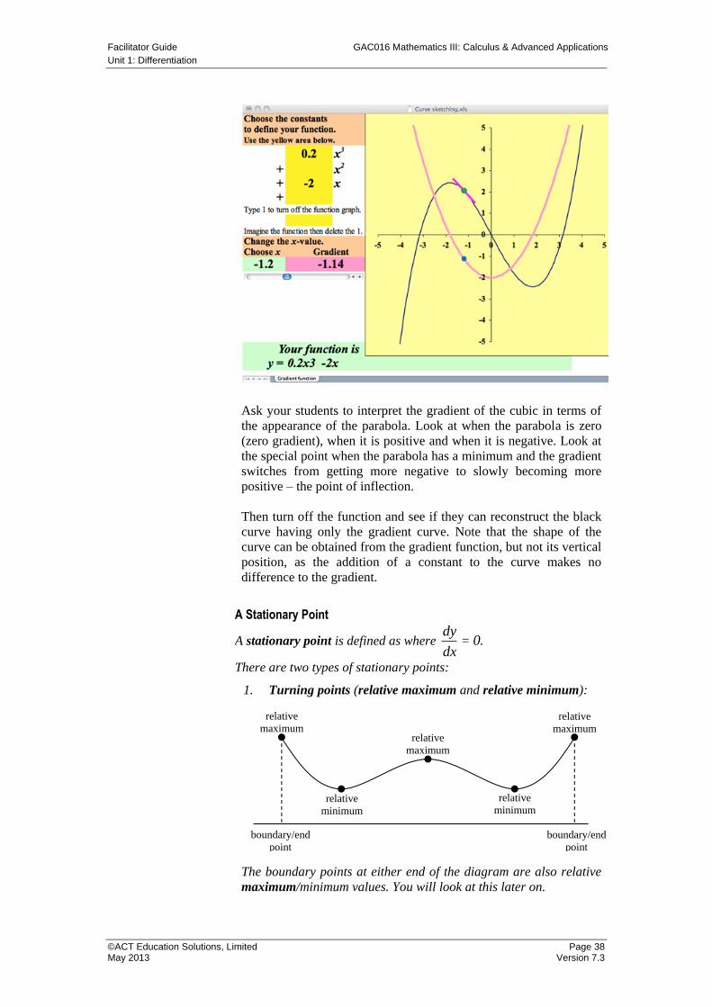
Ask your students to interpret the gradient of the cubic in terms of
the appearance of the parabola. Look at when the parabola is zero
(zero gradient), when it is positive and when it is negative. Look at
the special point when the parabola has a minimum and the gradient
switches from getting more negative to slowly becoming more
positive – the point of inflection.
Then turn off the function and see if they can reconstruct the black
curve having only the gradient curve. Note that the shape of the
curve can be obtained from the gradient function, but not its vertical
position, as the addition of a constant to the curve makes no
difference to the gradient.
A Stationary Point
A stationary point is defined as where dx
dy= 0.
There are two types of stationary points:
1. Turning points (relative maximum and relative minimum):
The boundary points at either end of the diagram are also relative
maximum/minimum values. You will look at this later on.
relative
maximum relative
maximum
relative
maximum
relative
minimum
relative
minimum
boundary/end
point
boundary/end
point
GAC016 Mathematics III: Calculus & Advanced Applications Facilitator Guide
Unit 1: Differentiation
Page 39 ©ACT Education Solutions, Limited Version 7.3 May 2013
Horizontal point of inflection (there are other points of inflection
where the tangents are not horizontal)
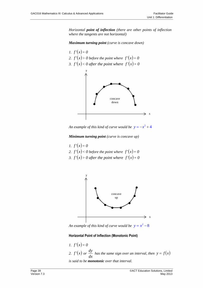
Maximum turning point (curve is concave down)
1. xf ' = 0
2. xf ' > 0 before the point where xf ' = 0
3. xf ' < 0 after the point where xf ' = 0
An example of this kind of curve would be 2 4y x
Minimum turning point (curve is concave up)
1. xf ' = 0
2. xf ' < 0 before the point where xf ' = 0
3. xf ' > 0 after the point where xf ' = 0
An example of this kind of curve would be 2 8y x
Horizontal Point of Inflection (Monotonic Point)
1. xf ' = 0
2. xf ' or dx
dy has the same sign over an interval, then xfy
is said to be monotonic over that interval.
x
y
concave
down
x
y
concave
up
Facilitator Guide GAC016 Mathematics III: Calculus & Advanced Applications
Unit 1: Differentiation
©ACT Education Solutions, Limited Page 40 May 2013 Version 7.3
Exploring Distance, Speed & Acceleration
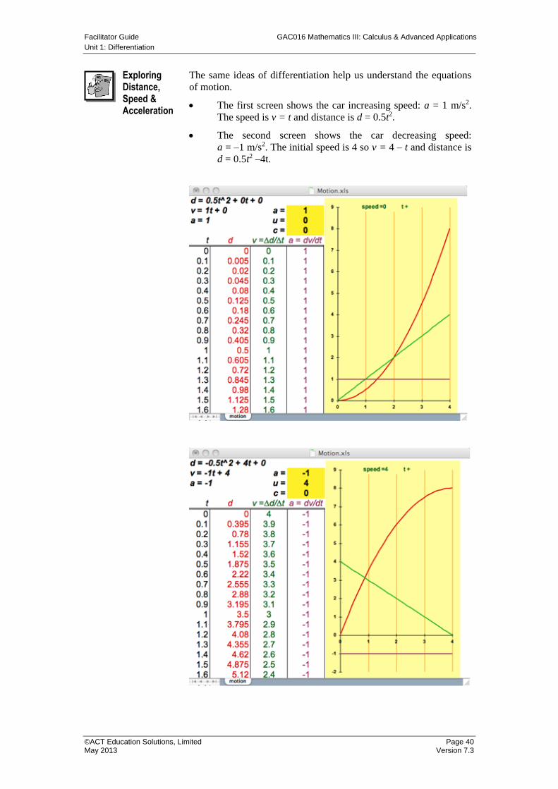
The same ideas of differentiation help us understand the equations
of motion.
The first screen shows the car increasing speed: a = 1 m/s2.
The speed is v = t and distance is d = 0.5t2.
The second screen shows the car decreasing speed:
a = –1 m/s2. The initial speed is 4 so v = 4 – t and distance is
d = 0.5t2 –4t.
GAC016 Mathematics III: Calculus & Advanced Applications Facilitator Guide
Unit 1: Differentiation
Page 41 ©ACT Education Solutions, Limited Version 7.3 May 2013
Task 1.7 1. Determine whether the curve 53 23 xxy is increasing,
horizontal or decreasing at x = 1.
2. Find any turning points on the curve
3536152 23 xxxy and determine if they are
maximum, minimum or neither.
3. Find the stationary points on the curve
6204 234 xxxxf and determine whether they are
maximum or minimum turning points.
4. If the curve 232 xaxxf has a stationary point where x
= 2, find the value of a and hence determine the type of turning
point.
5. If 3 5f x x has a monotonic point of inflection, determine
the coordinates for the point of inflection and describe the shape
of the graph of the function.
Solutions Task 1.7
1. dx
dy = 3x2 – 6x .
f ' (-1) = 9.
Increasing at x = -1
2. dx
dy = 6x2 + 30x + 36
= 6(x + 3 )(x + 2) = 0
x = -3, x = -2
Turning points at (-3, -62) and (-2, -63)
In the neighborhood of x = -2, dx
dy is – 0 +
minimum at (-2, -63)
In the neighborhood of x = -3, dx
dy is + 0 –
maximum at (-3, -62)
3. f ' (x) = 4x3 – 12x2 – 40x
= 4x( x – 5)(x + 2) = 0
x = 0, 5, -2
Turning points at (0 , 6), ( 5, -369), (-2, -26)
In the neighborhood of x = -2, dx
dy is – 0 +
minimum
Facilitator Guide GAC016 Mathematics III: Calculus & Advanced Applications
Unit 1: Differentiation
©ACT Education Solutions, Limited Page 42 May 2013 Version 7.3
In the neighborhood of x = 0, dx
dy is + 0 –
maximum
In the neighborhood of x = 5, dx
dy is – 0 +
minimum
4. f ' (x) = 2ax – 3 = 0
a = 3
4 when x = 2
Turning point occurs at (2, -1 )
In the neighborhood of x = 2, dx
dy is – 0 +
minimum
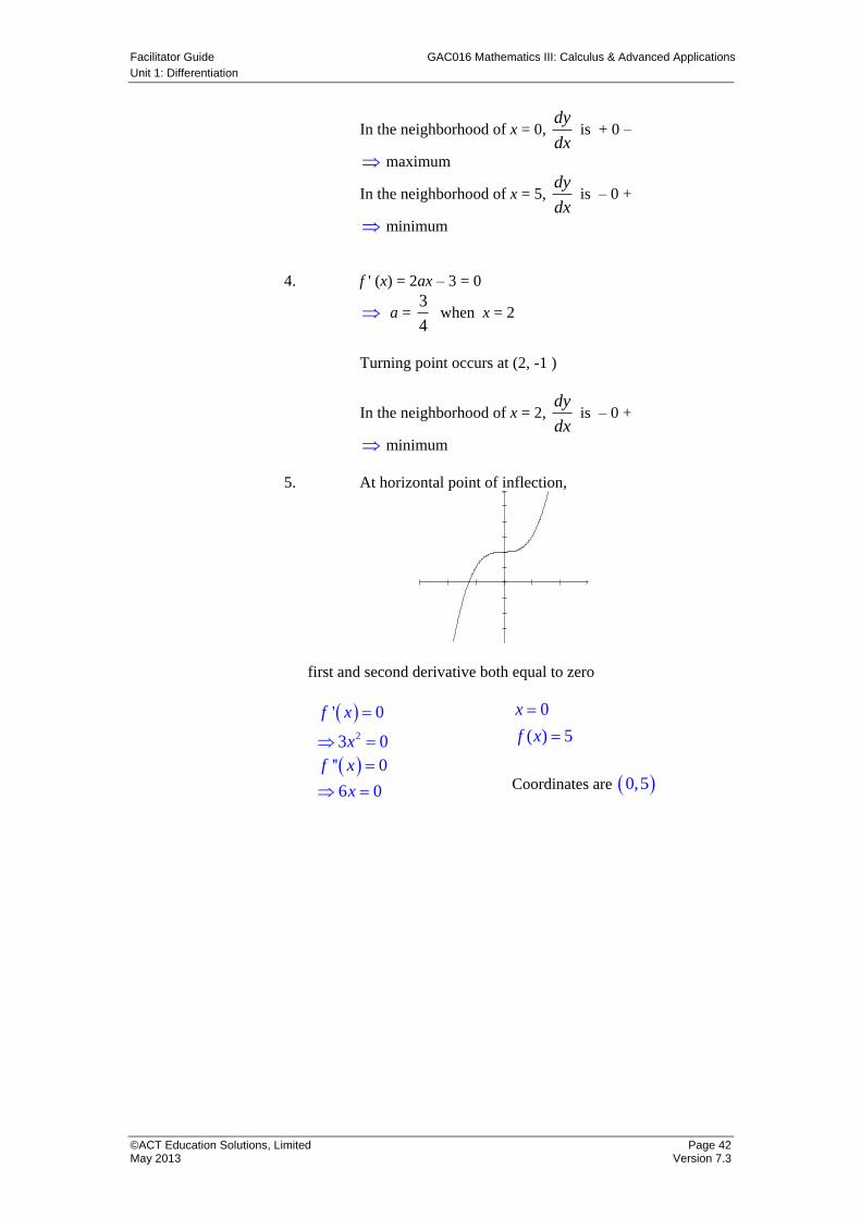
5. At horizontal point of inflection,
first and second derivative both equal to zero
' 0f x
23 0x
0
( ) 5
x
f x
'' 0f x
6 0x
Coordinates are 0,5
GAC016 Mathematics III: Calculus & Advanced Applications Facilitator Guide
Unit 1: Differentiation
Page 43 ©ACT Education Solutions, Limited Version 7.3 May 2013
Part J Differentiation – Circular Functions
Exploring Differentiation of Circular Functions
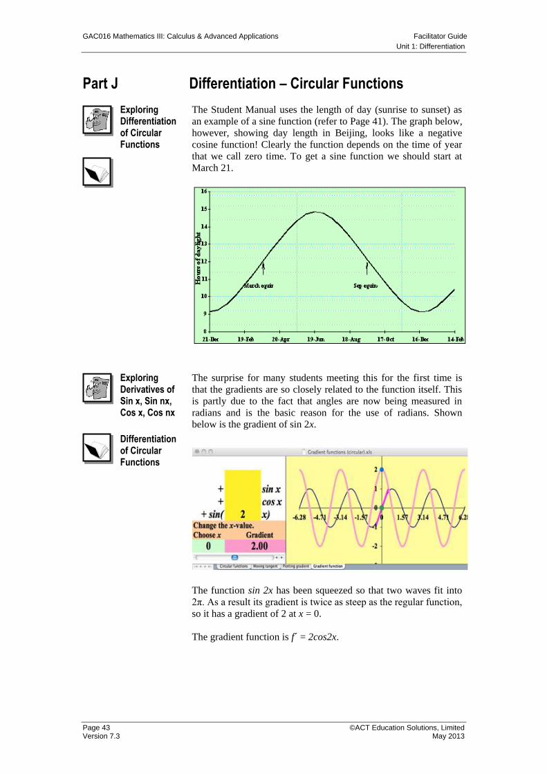
The Student Manual uses the length of day (sunrise to sunset) as
an example of a sine function (refer to Page 41). The graph below,
however, showing day length in Beijing, looks like a negative
cosine function! Clearly the function depends on the time of year
that we call zero time. To get a sine function we should start at
March 21.
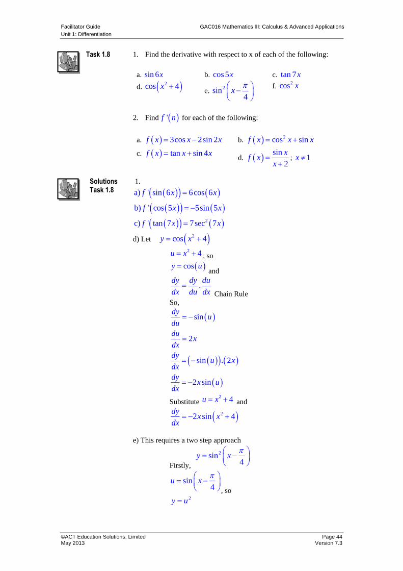
Exploring Derivatives of Sin x, Sin nx, Cos x, Cos nx
Differentiation of Circular Functions
The surprise for many students meeting this for the first time is
that the gradients are so closely related to the function itself. This
is partly due to the fact that angles are now being measured in
radians and is the basic reason for the use of radians. Shown
below is the gradient of sin 2x.
The function sin 2x has been squeezed so that two waves fit into
2π. As a result its gradient is twice as steep as the regular function,
so it has a gradient of 2 at x = 0.
The gradient function is f´ = 2cos2x.
Facilitator Guide GAC016 Mathematics III: Calculus & Advanced Applications
Unit 1: Differentiation
©ACT Education Solutions, Limited Page 44 May 2013 Version 7.3
Task 1.8 1. Find the derivative with respect to x of each of the following:
2. Find 'f n for each of the following:
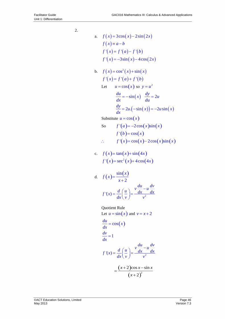
a. 3cos 2sin 2f x x x b. 2cos sinf x x x
c. tan sin 4f x x x d.
sin
2
xf x
x
; 1x
a. sin 6x b. cos5x c. tan 7x
d. 2cos 4x e.
2sin4
x
f.
2cos x
Solutions Task 1.8
1.
a) ' sin 6 6cos 6f x x
b) ' cos 5 5sin 5f x x
2c) ' tan 7 7sec 7f x x
d) Let 2cos 4y x
2 4u x , so
cosy u and
.dy dy du
dx du dx
Chain Rule
So,
sin
2
sin . 2
2 sin
dyu
du
dux
dx
dyu x
dx
dyx u
dx
Substitute 2 4u x and
22 sin 4dy
x xdx
e) This requires a two step approach
Firstly,
2sin4
y x
sin4
u x
, so
2y u
GAC016 Mathematics III: Calculus & Advanced Applications Facilitator Guide
Unit 1: Differentiation
Page 45 ©ACT Education Solutions, Limited Version 7.3 May 2013
Next need to solve
.du du dv
dx dv dx
; where
4v x
So,
1
cos
1 cos
cos
cos4
dv
dx
duv
dv
duv
dx
duv
dx
dux
dx
Chain Rule
Now,
2
cos4
2 .cos4
dyu
du
dux
dx
dyu x
dx
Chain Rule
Substitute sin4
u x
and
2sin cos4 4
dyx x
dx
f) Let 2cosy x
cosu x , so 2y u and
.dy dy du
dx du dx Chain Rule
2 sin
2 sin 2 sin
dy duu x
du dx
dyu x u x
dx
Substitute cosu x and
2cos sindy
x xdx
Facilitator Guide GAC016 Mathematics III: Calculus & Advanced Applications
Unit 1: Differentiation
©ACT Education Solutions, Limited Page 46 May 2013 Version 7.3
2.
a. 3cos 2sin 2f x x x
' ' '
' 3sin 4cos 2
f x a b
f x f a f b
f x x x
b. 2cos sinf x x x
' ' 'f x f a f b
Let cosu x so 2y u
sin 2
2 . sin 2 sin
du dyx u
dx du
dyu x u x
dx
Substitute cosu x
So ' 2cos sinf a x x
' cosf b x
' cos 2cos sinf x x x x
c. tan sin 4f x x x
2' sec 4cos 4f x x x
d. sin
2
xf x
x
2'( )
du dvv u
d u dx dxf xdx v v
Quotient Rule
Let sinu x and 2v x
cos
1
dux
dx
dv
dx
2'( )
du dvv u
d u dx dxf xdx v v
2
2 cos sin
2
x x x
x
GAC016 Mathematics III: Calculus & Advanced Applications Facilitator Guide
Unit 1: Differentiation
Page 47 ©ACT Education Solutions, Limited Version 7.3 May 2013
Part K Higher Derivatives
Significance of the Second Derivative
Task 1.9
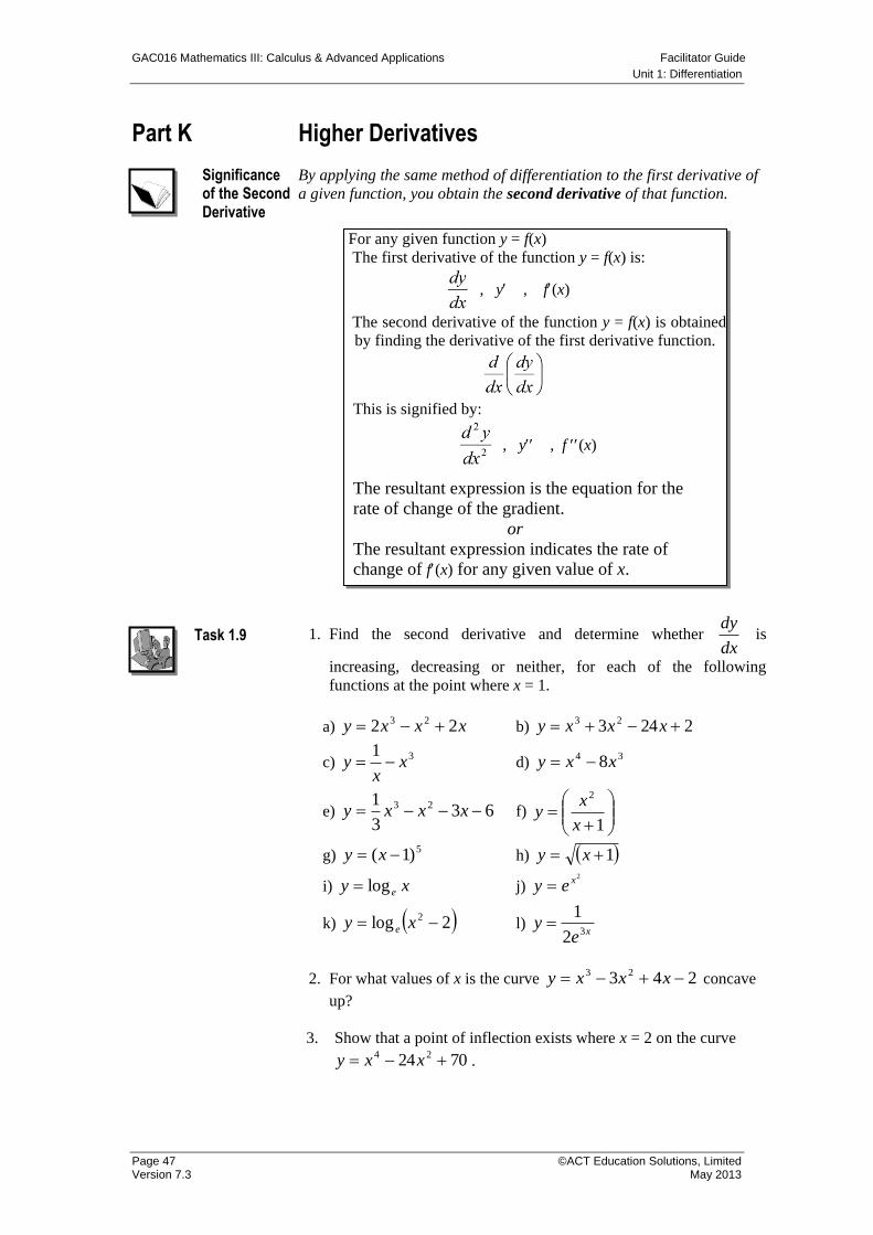
By applying the same method of differentiation to the first derivative of
a given function, you obtain the second derivative of that function.
1. Find the second derivative and determine whether dx
dy is
increasing, decreasing or neither, for each of the following
functions at the point where x = 1.
a) xxxy 22 23 b) 2243 23 xxxy
c) 31
xx
y d) 34 8xxy
e) 633
1 23 xxxy f)
1
2
x
xy
g) 5)1( xy h) 1 xy
i) xy elog j) 2xey
k) 2log 2 xy e l) xe
y32
1
2. For what values of x is the curve 243 23 xxxy concave
up?
3. Show that a point of inflection exists where x = 2 on the curve
7024 24 xxy .
For any given function y = f(x)
The first derivative of the function y = f(x) is:
, y , f(x)
The second derivative of the function y = f(x) is obtained
by finding the derivative of the first derivative function.
This is signified by:
, y , f (x)
The resultant expression is the equation for the
rate of change of the gradient.
or
The resultant expression indicates the rate of
change of f(x) for any given value of x.
Facilitator Guide GAC016 Mathematics III: Calculus & Advanced Applications
Unit 1: Differentiation
©ACT Education Solutions, Limited Page 48 May 2013 Version 7.3
Solutions Task 1.9
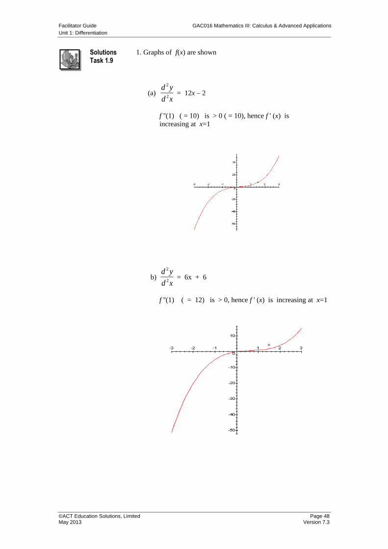
1. Graphs of f(x) are shown
(a) xd
yd2
2
= 12x – 2
f ''(1) ( = 10) is > 0 ( = 10), hence f ' (x) is
increasing at x=1
b) xd
yd2
2
= 6x + 6
f ''(1) ( = 12) is > 0, hence f ' (x) is increasing at x=1
GAC016 Mathematics III: Calculus & Advanced Applications Facilitator Guide
Unit 1: Differentiation
Page 49 ©ACT Education Solutions, Limited Version 7.3 May 2013
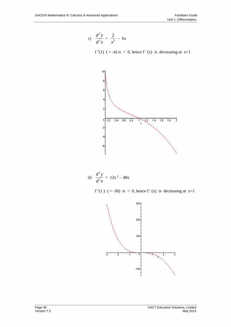
c) xd
yd2
2
= 3
2
x – 6x
f ''(1) ( = -4) is < 0, hence f ' (x) is decreasing at x=1
d) xd
yd2
2
= 12x 2 – 48x
f ''(1 ) ( = -36) is < 0, hence f ' (x) is decreasing at x=1
Facilitator Guide GAC016 Mathematics III: Calculus & Advanced Applications
Unit 1: Differentiation
©ACT Education Solutions, Limited Page 50 May 2013 Version 7.3
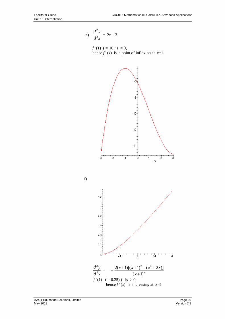
e) xd
yd2
2
= 2x – 2
f ''(1) ( = 0) is = 0,
hence f ' (x) is a point of inflexion at x=1
f)
xd
yd2
2
=
2 2
4
2( 1)[( 1) ( 2 )]
( 1)
x x x x
x
f ''(1) ( = 0.25) ) is > 0,
hence f ' (x) is increasing at x=1
GAC016 Mathematics III: Calculus & Advanced Applications Facilitator Guide
Unit 1: Differentiation
Page 51 ©ACT Education Solutions, Limited Version 7.3 May 2013
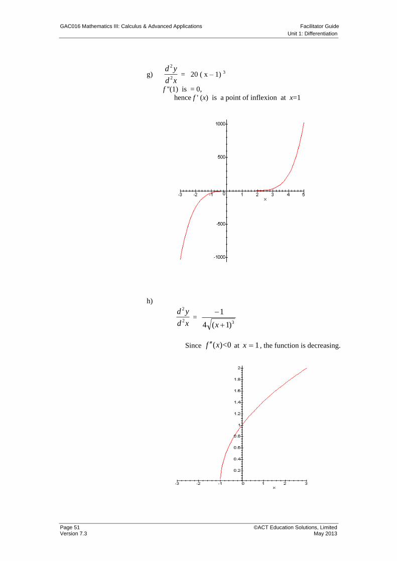
g) xd
yd2
2
= 20 ( x – 1) 3
f ''(1) is = 0,
hence f ' (x) is a point of inflexion at x=1
h)
xd
yd2
2
= 3)1(4
1
x
Since ( )<0f x at 1x , the function is decreasing.
Facilitator Guide GAC016 Mathematics III: Calculus & Advanced Applications
Unit 1: Differentiation
©ACT Education Solutions, Limited Page 52 May 2013 Version 7.3
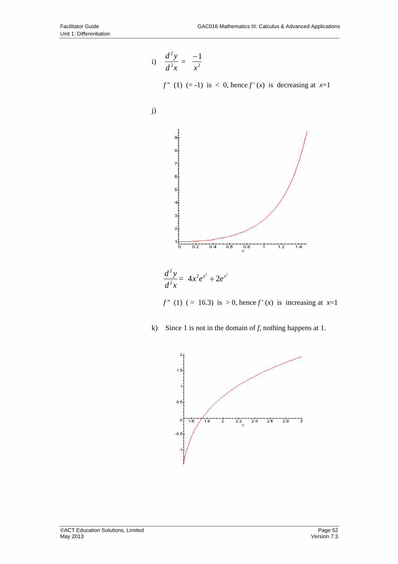
i) xd
yd2
2
= 2
1
x
f '' (1) (= -1) is < 0, hence f ' (x) is decreasing at x=1
j)
2 2
22
2= 4 2x xd y
x e ed x
f '' (1) ( = 16.3) is > 0, hence f ' (x) is increasing at x=1
k) Since 1 is not in the domain of f, nothing happens at 1.
GAC016 Mathematics III: Calculus & Advanced Applications Facilitator Guide
Unit 1: Differentiation
Page 53 ©ACT Education Solutions, Limited Version 7.3 May 2013
l) xd
yd2
2
= 3
9
2 xe
f ''(1) (= 0.224) is > 0,
hence f ' (x) is increasing at x=1
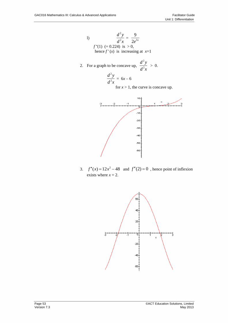
2. For a graph to be concave up, xd
yd2
2
> 0.
xd
yd2
2
= 6x – 6
for x > 1, the curve is concave up.
3. 2( ) 12 48 f x x and (2) 0f , hence point of inflexion
exists where x = 2.
Facilitator Guide GAC016 Mathematics III: Calculus & Advanced Applications
Unit 1: Differentiation
©ACT Education Solutions, Limited Page 54 May 2013 Version 7.3
Part L Curve Sketching
Exploring Curve Sketching
Fundament-als of Curve Sketching
Task 1.10
Common Conventions (from Student Manual p. 46) 1. All axes must be labelled, where possible.
2. Scales should be appropriately selected for each axis.
3. The size of the graph should be sufficient to reasonably convey,
in a clear and concise manner, all relevant information.
4. The graph of a function should be labelled with its equation.
5. The coordinates of turning points, points of inflection,
asymptotes, points of intersection, boundary points and any other
important information should be clearly identified.
6. Where there are more than one function being charted on the
same set of axes, arrows may be required to clearly identify
relevant information.
7. All graphs should be drawn with a reasonable attempt to
accurately represent the shape and features of the graph.
Sketch the graph for each of the following functions on a separate
number plane. Show and label:
- stationary points
- inflection points
- boundary values (if given a set domain)
- absolute maximum and minimum (if given a set domain)
1. 193 23 xxxy 2. 72492 23 xxxy
3 x 6
3. 3125 xxy 4.
23 xxy
2 x 4
5. 12 34 xxy 6. xxy 43
2 x 5
7. 36 24 xxy 8. 1
2
x
xy ; 5 x 1
9.3
3
x
xy ; 5 x 5 10.
1
12
x
xxy
11. 6sin(30 ), 6 6y x x
12. 24ln( )y x
Challenge Question
13. cos(30 ) 2y x , 6 6x
GAC016 Mathematics III: Calculus & Advanced Applications Facilitator Guide
Unit 1: Differentiation
Page 55 ©ACT Education Solutions, Limited Version 7.3 May 2013
Solutions Task 1.10
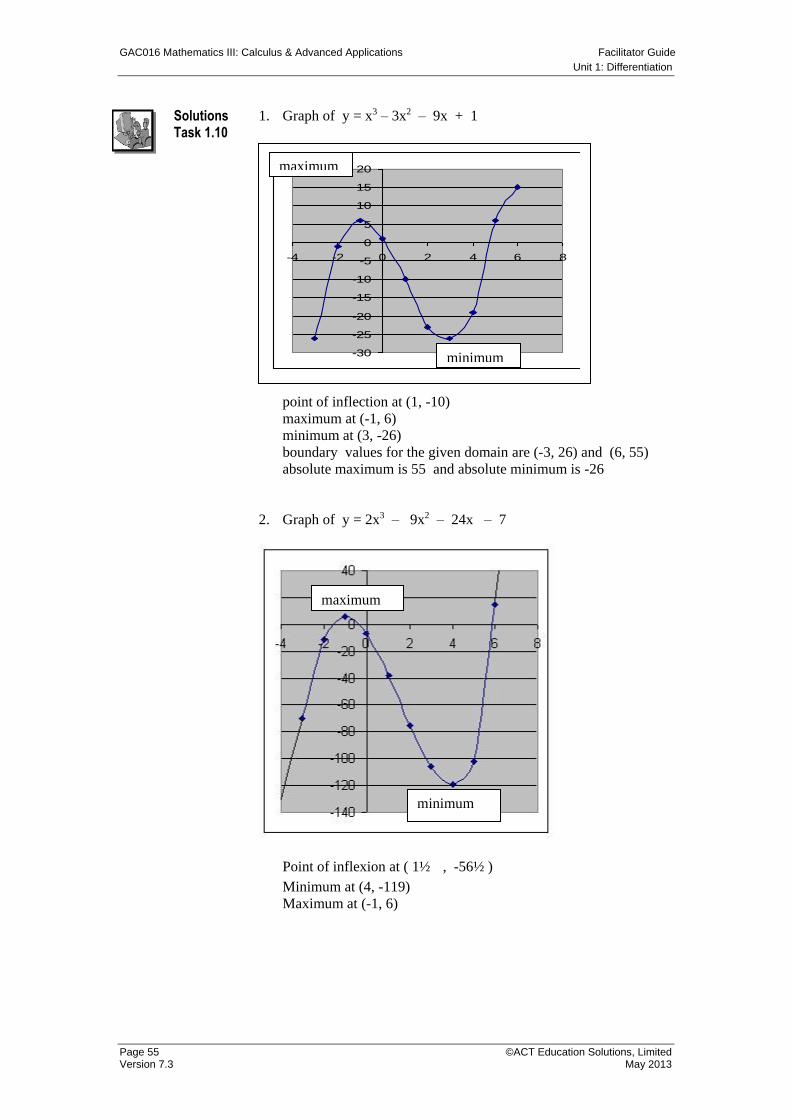
1. Graph of y = x3 – 3x2 – 9x + 1
point of inflection at (1, -10)
maximum at (-1, 6)
minimum at (3, -26)
boundary values for the given domain are (-3, 26) and (6, 55)
absolute maximum is 55 and absolute minimum is -26
2. Graph of y = 2x3 – 9x2 – 24x – 7
Point of inflexion at ( 1½ , -56½ )
Minimum at (4, -119)
Maximum at (-1, 6)
maximum
minimum
-30
-25
-20
-15
-10
-5
0
5
10
15
20
-4 -2 0 2 4 6 8 Series1
minimum
maximum
Facilitator Guide GAC016 Mathematics III: Calculus & Advanced Applications
Unit 1: Differentiation
©ACT Education Solutions, Limited Page 56 May 2013 Version 7.3
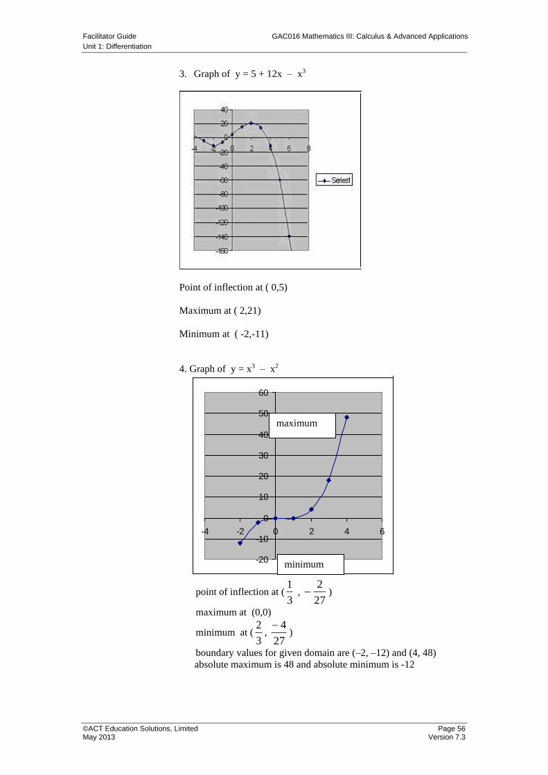
3. Graph of y = 5 + 12x – x3
Point of inflection at ( 0,5)
Maximum at ( 2,21)
Minimum at ( -2,-11)
4. Graph of y = x3 – x2
point of inflection at (1
3 ,
27
2 )
maximum at (0,0)
minimum at (2
3,
27
4)
boundary values for given domain are (–2, –12) and (4, 48)
absolute maximum is 48 and absolute minimum is -12
-20
-10
0
10
20
30
40
50
60
-4 -2 0 2 4 6
Series1
minimum
maximum
GAC016 Mathematics III: Calculus & Advanced Applications Facilitator Guide
Unit 1: Differentiation
Page 57 ©ACT Education Solutions, Limited Version 7.3 May 2013
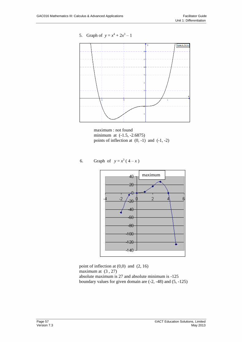
5. Graph of y = x4 + 2x3 – 1
maximum : not found
minimum at (-1.5, -2.6875)
points of inflection at (0, -1) and (-1, -2)
6. Graph of y = x3 ( 4 – x )
point of inflection at (0,0) and (2, 16)
maximum at (3 , 27)
absolute maximum is 27 and absolute minimum is -125
boundary values for given domain are (-2, -48) and (5, -125)
maximum
Facilitator Guide GAC016 Mathematics III: Calculus & Advanced Applications
Unit 1: Differentiation
©ACT Education Solutions, Limited Page 58 May 2013 Version 7.3
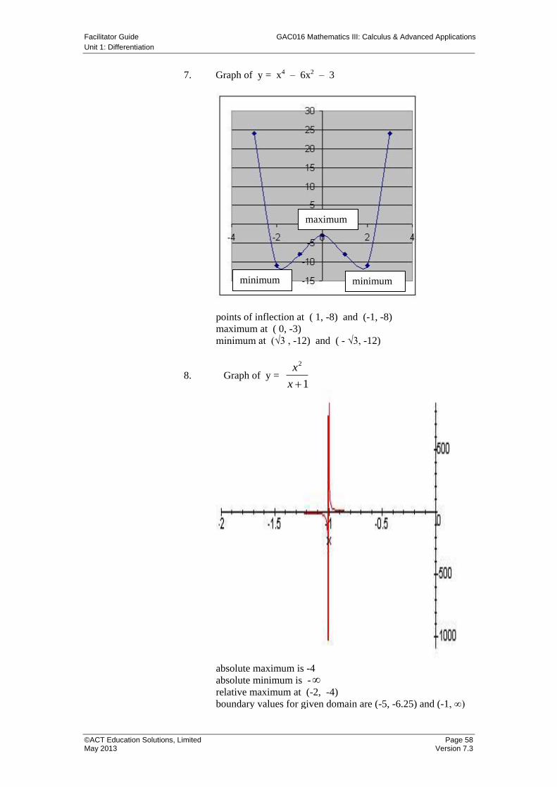
7. Graph of y = x4 – 6x2 – 3
points of inflection at ( 1, -8) and (-1, -8)
maximum at ( 0, -3)
minimum at (√3 , -12) and ( - √3, -12)
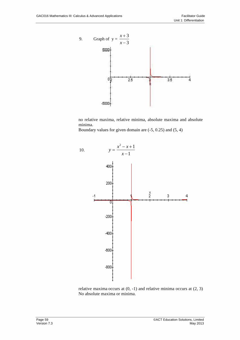
8. Graph of y = 1
2
x
x
absolute maximum is -4
absolute minimum is -
relative maximum at (-2, -4)
boundary values for given domain are (-5, -6.25) and (-1, ∞)
minimum minimum
maximum
GAC016 Mathematics III: Calculus & Advanced Applications Facilitator Guide
Unit 1: Differentiation
Page 59 ©ACT Education Solutions, Limited Version 7.3 May 2013
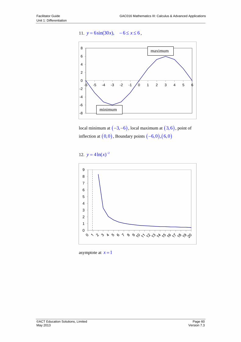
9. Graph of y = 3
3
x
x
no relative maxima, relative minima, absolute maxima and absolute
minima.
Boundary values for given domain are (-5, 0.25) and (5, 4)
10. 1
12
x
xxy
relative maxima occurs at (0, -1) and relative minima occurs at (2, 3)
No absolute maxima or minima.
Facilitator Guide GAC016 Mathematics III: Calculus & Advanced Applications
Unit 1: Differentiation
©ACT Education Solutions, Limited Page 60 May 2013 Version 7.3
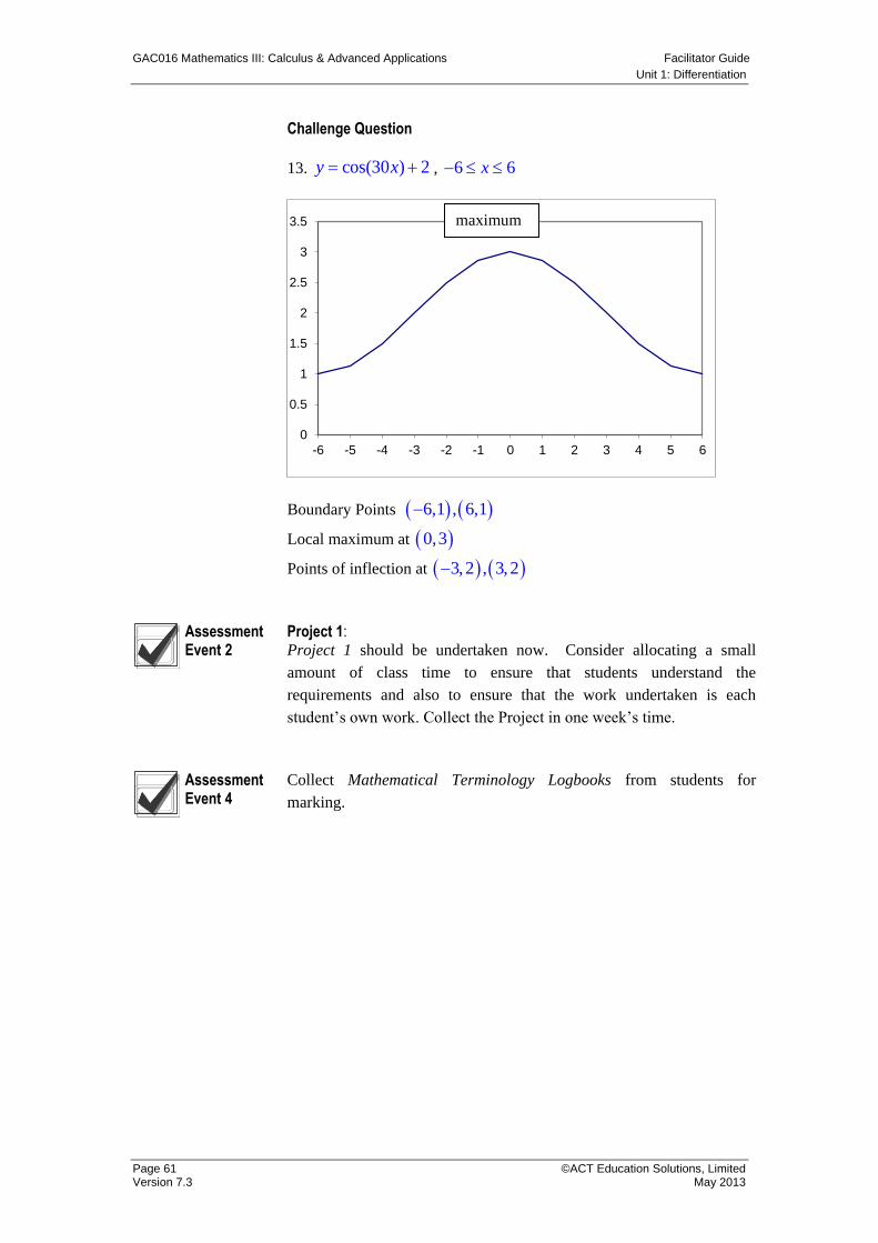
11. 6sin(30 ), 6 6y x x ,
local minimum at 3, 6 , local maximum at 3,6 , point of
inflection at 0,0 , Boundary points 6,0 , 6,0
12. 24ln( )y x
asymptote at 1x
-8
-6
-4
-2
0
2
4
6
8
-6 -5 -4 -3 -2 -1 0 1 2 3 4 5 6
0
1
2
3
4
5
6
7
8
9
maximum
minimum
GAC016 Mathematics III: Calculus & Advanced Applications Facilitator Guide
Unit 1: Differentiation
Page 61 ©ACT Education Solutions, Limited Version 7.3 May 2013
Challenge Question
13. cos(30 ) 2y x , 6 6x
Boundary Points 6,1 , 6,1
Local maximum at 0,3
Points of inflection at 3,2 , 3,2
Assessment Event 2
Project 1: Project 1 should be undertaken now. Consider allocating a small
amount of class time to ensure that students understand the
requirements and also to ensure that the work undertaken is each
student’s own work. Collect the Project in one week’s time.
Assessment Event 4
Collect Mathematical Terminology Logbooks from students for
marking.
0
0.5
1
1.5
2
2.5
3
3.5
-6 -5 -4 -3 -2 -1 0 1 2 3 4 5 6
maximum

GAC016 Mathematics III: Calculus & Advanced Applications Facilitator Guide
Unit 2: Integration
Page 63 ©ACT Education Solutions, Limited Version 7.3 May 2013
Unit 2: Integration
Part A Unit Introduction
Part B Terminology Introduced
Part C The Primitive Function and Indefinite Integrals
Part D Definite Integrals and the Area under a Curve
Part E The Volume of Rotation
Part A Unit Introduction
Overview In this unit, students will learn to apply appropriate methods of integral
calculus to solving various numerical and graphical problems.
In this unit, students will learn to:
select appropriate methods of integral calculus
calculate the area enclosed by a given curve
calculate the length of a curve
calculate the volume enclosed by a given surface.
This unit includes a series of tasks that students will work through to
practise the course material. They will be expected to complete some
work in their own time. You will guide them through the unit.
Assessment Event 1
In-class Test should be administered at the end of Unit 2. Note that this
is an in-class test under test conditions.
Assessment Event 4
Assessment Reminder: You must collect students’ Mathematical
Terminology Logbooks at the end of each unit.
Facilitator Guide GAC016 Mathematics III: Calculus & Advanced Applications
Unit 2: Integration
©ACT Education Solutions, Limited Page 64 May 2013 Version 7.3
Part B Terminology Introduced
By the end of this unit, students need to know the meanings of these
terms. The terms are bolded in the first instance they occur. Please
make sure students understand the definitions of new terminology
and include these words in their Mathematical Terminology Logbook.
Summary of terms
primitive function
lower limit
volume of rotation
intervals
definite integral
integrand
approximation
constant of integration
integration
trapezoidal rule
subintervals
fundamental theorem
variable of integration
upper limit
bounded
Simpson’s rule
indefinite integral
anti-derivative
numerical methods
GAC016 Mathematics III: Calculus & Advanced Applications Facilitator Guide
Unit 2: Integration
Page 65 ©ACT Education Solutions, Limited Version 7.3 May 2013
Part C The Primitive Function and Indefinite Integrals
Integration
Anti-Derivatives
Task 2.1
The Primitive Function (Refer to Student Manual p. 58)
The primitive of a function is the name usually given to the anti-
derivative. It is the original function from which the derivative was
found.
So far you have only looked at the concept of what the primitive
function is in relation to the derivative. Within the examples on the
previous page you may have noticed a pattern/rule emerging when
finding the primitive from the function of the derivative.
1. Find the primitive function of:
a) 3 b) 2x c) 9x2
d) 54 x e) 243 3 xx f) 24 310 xx
g) 463 x h)
x
1 i) 7
5
x
2. Find f (x) if:
a) f (x) = xx 29 b) f (x) = 346 35 xx
c) f (x) = 483 x d) f (x) = 43 xx
e) f (x) = 2
1
3x f) f (x) = 3 2x
An anti-derivative of a function f(x) is another function F(x)
such that:
F(x) = f(x)
or
Any two anti-derivatives of a function differ only by a constant.
Rules:
If then + C, where k is any constant
If then , n 1
If then , n 1
Facilitator Guide GAC016 Mathematics III: Calculus & Advanced Applications
Unit 2: Integration
©ACT Education Solutions, Limited Page 66 May 2013 Version 7.3
3. Express y in terms of x if:
a) 54 3 xdx
dy b)
24
21
xxdx
dy
c) 9
2
5x
x
dx
dy d) xx
dx
dy 3
e) 3
321
x
x
dx
dy f)
2
123 23
x
xxx
dx
dy
4. Given that f (x) = 116 x and f (3) = 19, find an expression for
f(x).
5. Given that f (t) = 24t and f (6) = 22, find f (1).
6. If y = (x 3)2 and x = 7 when y = 0, find x when y = 4.
7. Given that f (x) = 5x4, f (0) = 3 and f (–1) = 1, find f (2).
8. If the gradient of the tangent to a curve is given by 12 x and the
curve passes through the point (3, 0), find the equation of the
curve.
9. The rate of change of V with respect to t is given by
212 tdt
dV
If V = 5 when t = 05, find V when t = 5.
Solutions Task 2.1
1. Using Rules
: if f '(x) = k then f (x) = kx
: if f '(x) = xn then f (x) = 1
1
n
xn
+ C
: if f '(x) = nbax )( then f (x) =
)1(
)( 1
na
bax n
+ C
a) 3x + C
b) x2 + C
c) 3x3 + C
d) 2x2 + 5x + C
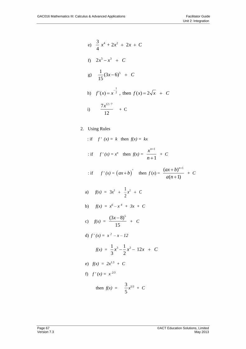
GAC016 Mathematics III: Calculus & Advanced Applications Facilitator Guide
Unit 2: Integration
Page 67 ©ACT Education Solutions, Limited Version 7.3 May 2013
e) 4 23
+ 2 2 4
x x x C
f) 5 32 x x C
g) 51
(3 6) 15
x C
h)
1
2( ) , then ( ) 2 f x x f x x C
i) 12
7 7/12x + C
2. Using Rules
: if f ' (x) = k then f(x) = kx
: if f ' (x) = xn then f(x) = 1
1
n
xn
+ C
: if f ' (x) = n
ax b then f (x) = )1(
)( 1
na
bax n
+ C
a) f(x) = 3 21
3 2
x x C
b) f(x) = x6 – x 4 + 3x + C
c) f(x) = 15
)83( 5x + C
d) f ' (x) = x 2 – x – 12
f(x) = 3 21 1
12 3 2
x x x C
e) f(x) = 2x1.5 + C
f) f ' (x) = x 2/3
then f(x) = 5
3x5/3 + C
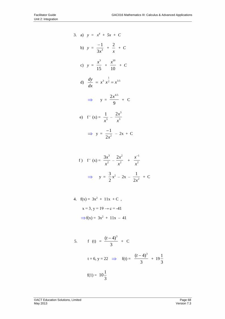
Facilitator Guide GAC016 Mathematics III: Calculus & Advanced Applications
Unit 2: Integration
©ACT Education Solutions, Limited Page 68 May 2013 Version 7.3
3. a) y = x4 + 5x + C
b) y = 33
1
x
+
x
2 + C
c) y = 15
3x +
10
10x + C
d) dx
dy
1
3 3.52 x x x
y = 9
2 5.4x + C
e) f ' (x) = 3
1
x –
3
32
x
x
y = 22
1
x
– 2x + C
f ) f ' (x) = 2
33
x
x –
2
22
x
x +
2
1
x
x
y = 2
3x2 – 2x –
22
1
x + C
4. f(x) = 3x2 + 11x + C ,
x = 3, y = 19 → c = -41
f(x) = 3x2 + 11x – 41
5. f (t) = 3
)4( 3t + C
t = 6, y = 22 f(t) = 3
)4( 3t + 19
1
3
f(1) = 1
103
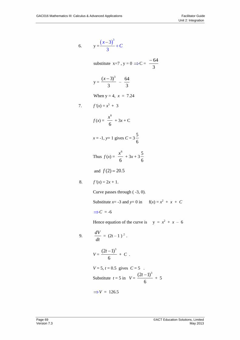
GAC016 Mathematics III: Calculus & Advanced Applications Facilitator Guide
Unit 2: Integration
Page 69 ©ACT Education Solutions, Limited Version 7.3 May 2013
6. y =
33
3
xC
substitute x=7 , y = 0 C = 3
64
y = 3
)3( 3x –
64
3
When y = 4, x = 7.24
7. f '(x) = x5 + 3
f (x) = 6
6x + 3x + C
x = -1, y= 1 gives C = 36
5
Thus f (x) = 6
6x + 3x + 3
6
5
and (2) 20.5f
8. f '(x) = 2x + 1.
Curve passes through ( -3, 0).
Substitute x= -3 and y= 0 in f(x) = x2 + x + C
C = -6
Hence equation of the curve is y = x2 + x – 6
9. dt
dV = (2t – 1 ) 2 .
V = 6
)12( 3t + C .
V = 5, t = 0.5 gives C = 5 .
Substitute t = 5 in V = 6
)12( 3t + 5
V = 126.5
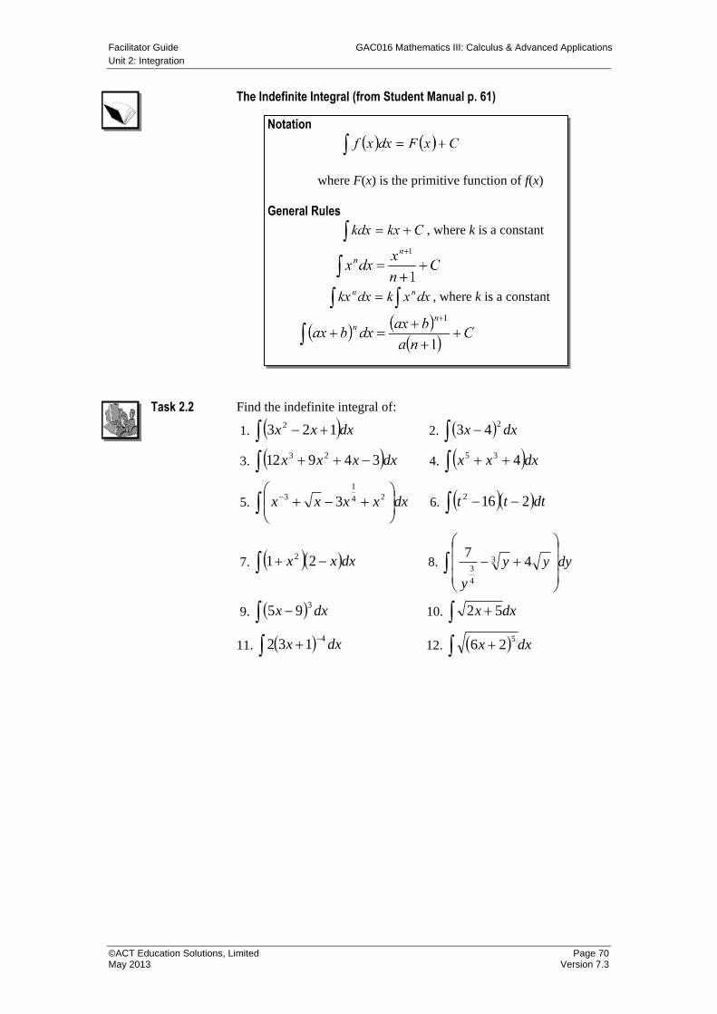
Facilitator Guide GAC016 Mathematics III: Calculus & Advanced Applications
Unit 2: Integration
©ACT Education Solutions, Limited Page 70 May 2013 Version 7.3
The Indefinite Integral (from Student Manual p. 61)
Task 2.2 Find the indefinite integral of:
1. dxxx 123 2 2. dxx
243
3. dxxxx 34912 23 4. dxxx 435
5.
dxxxxx 24
1
3 3 6. dttt 2162
7. dxxx 21 2 8.
dyyy
y
47
3
4
3
9. dxx3
95 10. dxx 52
11.
dxx4
132 12. dxx5
26
Notation
where F(x) is the primitive function of f(x)
General Rules
, where k is a constant
, where k is a constant
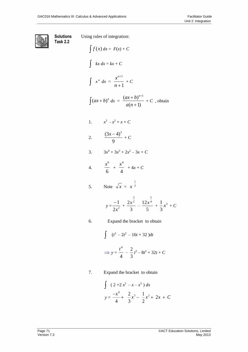
GAC016 Mathematics III: Calculus & Advanced Applications Facilitator Guide
Unit 2: Integration
Page 71 ©ACT Education Solutions, Limited Version 7.3 May 2013
Solutions Task 2.2
Using rules of integration:
)(xf dx = F(x) + C
kx dx = kx + C
x n dx = 1
1
n
xn
+ C
nbax )( dx = )1(
)( 1
na
bax n
+ C , obtain
1. x3 - x2 + x + C
2. 9
)43( 3x + C
3. 3x4 + 3x3 + 2x2 – 3x + C
4. 6
6x +
4
4x + 4x + C
5. Note x =
1
2 x
y =22
1
x
+
3
22
3
x –
5
412
5
x +
31
3x + C
6. Expand the bracket to obtain
(t3 – 2t2 – 16t + 32 )dt
y = 4
4t –
2
3t3 – 8t2 + 32t + C
7. Expand the bracket to obtain
( 2 +2 x2 – x – x3 ) dx
y =
43 22 1
2 4 3 2
xx x x C
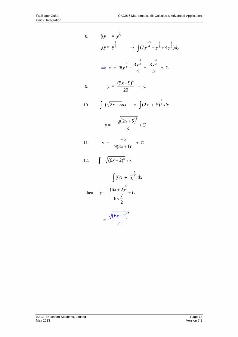
Facilitator Guide GAC016 Mathematics III: Calculus & Advanced Applications
Unit 2: Integration
©ACT Education Solutions, Limited Page 72 May 2013 Version 7.3
8. 3 y =
1
3y
1
2= y y →
3 1 1
4 3 2(7 4 )y y y dy
41 34
3 28
4
yx y +
3
28
3
y + C
9. y = 20
)95( 4x + C
10. dxx 52( =
1
2(2 5) x dx
y =
32 5
3
xC
11. y = 3)13(9
2
x + C
12. 5)26( x dx
=
5
2 (6 5) x dx
then y =
7
2(6 2)
76
2
xC
=
76 2
21
x
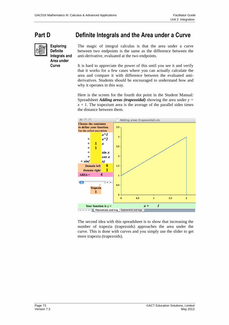
GAC016 Mathematics III: Calculus & Advanced Applications Facilitator Guide
Unit 2: Integration
Page 73 ©ACT Education Solutions, Limited Version 7.3 May 2013
Part D Definite Integrals and the Area under a Curve
Exploring Definite Integrals and Area under Curve
The magic of integral calculus is that the area under a curve
between two endpoints is the same as the difference between the
anti-derivative, evaluated at the two endpoints.
It is hard to appreciate the power of this until you see it and verify
that it works for a few cases where you can actually calculate the
area and compare it with difference between the evaluated anti-
derivatives. Students should be encouraged to understand how and
why it operates in this way.
Here is the screen for the fourth dot point in the Student Manual:
Spreadsheet Adding areas (trapezoidal) showing the area under y =
x + 1. The trapezium area is the average of the parallel sides times
the distance between them.
The second idea with this spreadsheet is to show that increasing the
number of trapezia (trapezoids) approaches the area under the
curve. This is done with curves and you simply use the slider to get
more trapezia (trapezoids).
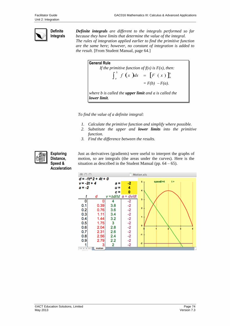
Facilitator Guide GAC016 Mathematics III: Calculus & Advanced Applications
Unit 2: Integration
©ACT Education Solutions, Limited Page 74 May 2013 Version 7.3
Definite Integrals
Definite integrals are different to the integrals performed so far
because they have limits that determine the value of the integral.
The rules of integration applied earlier to find the primitive function
are the same here; however, no constant of integration is added to
the result. [From Student Manual, page 64.] To find the value of a definite integral:
1. Calculate the primitive function and simplify where possible.
2. Substitute the upper and lower limits into the primitive
function.
3. Find the difference between the results.
Exploring Distance, Speed & Acceleration
Just as derivatives (gradients) were useful to interpret the graphs of
motion, so are integrals (the areas under the curves). Here is the
situation as described in the Student Manual (pp. 64 – 65).
General Rule If the primitive function of f(x) is F(x), then:
= F(b) F(a).
where b is called the upper limit and a is called the
lower limit.
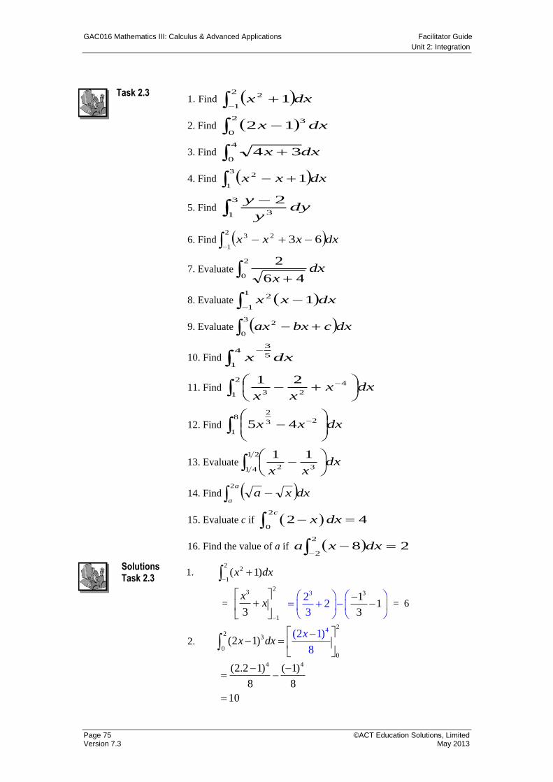
GAC016 Mathematics III: Calculus & Advanced Applications Facilitator Guide
Unit 2: Integration
Page 75 ©ACT Education Solutions, Limited Version 7.3 May 2013
Task 2.3 1. Find
2
1
2 1 dxx
2. Find 2
0
312 dxx
3. Find 4
034 dxx
4. Find 3
1
2 1 dxxx
5. Find 3
1 3
2dy
y
y
6. Find 2
1
23 63 dxxxx
7. Evaluate
2
0 46
2dx
x
8. Evaluate 1
1
2 1 dxxx
9. Evaluate 3
0
2 dxcbxax
10. Find 4
1
5
3
dxx
11. Find
2
1
4
23
21dxx
xx
12. Find
8
1
23
2
45 dxxx
13. Evaluate
21
41 32
11dx
xx
14. Find a
adxxa
2
15. Evaluate c if 2
02 4
c
x dx
16. Find the value of a if 2
228 dxxa
Solutions Task 2.3
1. 1. 2
1
2 )1( dxx
=
2
1
3
3
x
x
3322
3
11
3
= 6
2.
22
3
00
4(2 1)
8(2 1)x
xdx
4 4(2.2 1) ( 1)
8 8
10
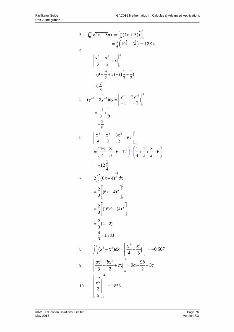
Facilitator Guide GAC016 Mathematics III: Calculus & Advanced Applications
Unit 2: Integration
©ACT Education Solutions, Limited Page 76 May 2013 Version 7.3
3. ∫ √4𝑥 + 3𝑑𝑥4
0= [
1
6(4𝑥 + 3)
3
2]0
4
=1
6ቀ19
3
2 − 33
2ቁ ≅ 12.94
4.
3
26
)2
1
3
11()3
2
99(
x2
x
3
x3
1
23
5.
3
1
2132
2
y2
1
ydy)y2y(
9
2
9
1
3
1
6.
2
1
234
x62
x3
3
x
4
x
16 8 1 1 36 12 6
4 3 4 3 2
312
4
7.
12
2
02 (6 4)x dx
333.13
4
)24(3
2
)4()16(3
2
)4x6(3
2
2
1
2
1
2
0
2
1
8.
14 31
3 2
11
( ) 0.6674 3
x xx x dx
9.
33 2
0
99 3
3 2 2
ax bx bcx a c
10.
42
5
1
2
5
x
= 1.853
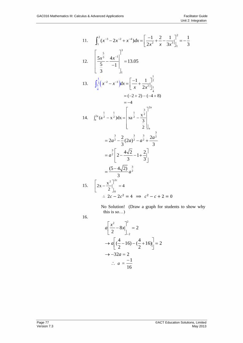
GAC016 Mathematics III: Calculus & Advanced Applications Facilitator Guide
Unit 2: Integration
Page 77 ©ACT Education Solutions, Limited Version 7.3 May 2013
11.
22
3 2 4
2 31
1
1 2 1 1( 2 )
2 3 3x x x dx
x x x
12.
35
13
1
5 413.05
5 1
3
x x
13. 1
22 3
21
4
1
21
4
1 1
2x x dx
x x
4
)84()22(
14.
a2
a
2
3
2
1
2
1
a2
a2
1
2
3
xxadx)xa(
33 3 3 22 2 2
3
2
3
2
2 22 (2 )
3 3
4 2 22 1
3 3
(5 4 2)
3
aa a a
a
a
15. 42
xx2
c2
0
2
∴ 2𝑐 − 2𝑐2 = 4 ⟹ 𝑐2 − 𝑐 + 2 = 0
No Solution! (Draw a graph for students to show why
this is so…)
16.
232
2)162
4()16
2
4(
282
2
2
2
a
a
xx
a
a = 16
1
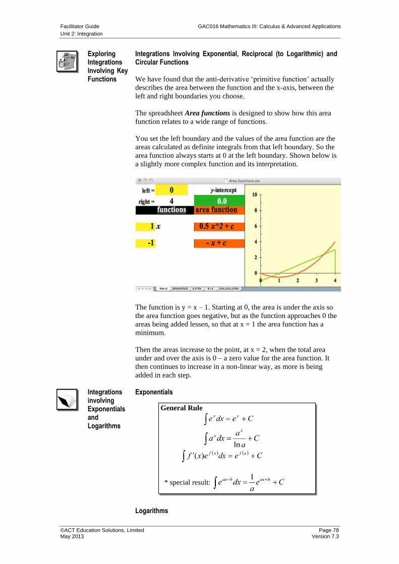
Facilitator Guide GAC016 Mathematics III: Calculus & Advanced Applications
Unit 2: Integration
©ACT Education Solutions, Limited Page 78 May 2013 Version 7.3
Exploring Integrations Involving Key Functions
Integrations Involving Exponential, Reciprocal (to Logarithmic) and Circular Functions
We have found that the anti-derivative ‘primitive function’ actually
describes the area between the function and the x-axis, between the
left and right boundaries you choose.
The spreadsheet Area functions is designed to show how this area
function relates to a wide range of functions.
You set the left boundary and the values of the area function are the
areas calculated as definite integrals from that left boundary. So the
area function always starts at 0 at the left boundary. Shown below is
a slightly more complex function and its interpretation.
The function is y = x – 1. Starting at 0, the area is under the axis so
the area function goes negative, but as the function approaches 0 the
areas being added lessen, so that at x = 1 the area function has a
minimum.
Then the areas increase to the point, at x = 2, when the total area
under and over the axis is 0 – a zero value for the area function. It
then continues to increase in a non-linear way, as more is being
added in each step.
Integrations involving Exponentials and Logarithms
Exponentials
Logarithms
General Rule
* special result:
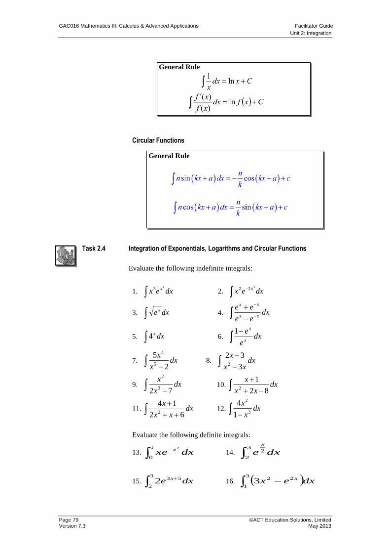
GAC016 Mathematics III: Calculus & Advanced Applications Facilitator Guide
Unit 2: Integration
Page 79 ©ACT Education Solutions, Limited Version 7.3 May 2013
Circular Functions
Task 2.4 Integration of Exponentials, Logarithms and Circular Functions
Evaluate the following indefinite integrals:
1. dxex x43 2.
dxex x322
3. dxe x 4.
dx
ee
eexx
xx
5. dxx4 6.
dxe
ex
x1
7. dx
x
x
2
55
4
8.
dx
xx
x
3
322
9. dx
x
x
72 3
2
10.
dx
xx
x
82
12
11.
dx
xx
x
62
142
12. dx
x
x3
2
1
4
Evaluate the following definite integrals:
13.
1
0
2
dxxe x 14.
3
2
2 dxe
x
15.
3
2
532 dxe x 16.
3
1
223 dxex x
General Rule
General Rule
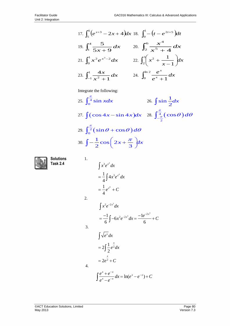
Facilitator Guide GAC016 Mathematics III: Calculus & Advanced Applications
Unit 2: Integration
©ACT Education Solutions, Limited Page 80 May 2013 Version 7.3
17. 6
5
3 42 dxxe x 18.
1
0
52 dtet t
19.
4
1 95
5dx
x 20.
6
2 5
4
4dx
x
x
21.
1
0
22 3
dxex x 22.
3
2
2
1
1dx
xx
23.
1
1 2 1
4dx
x
x 24.
2ln
0 1dx
e
ex
x
Integrate the following:
25. 4
0sin xdx
26. 1
sin2
dx
27. cos 4 sin 4x x dx 28. 4
2
cos d
29. 2
0sin cos d
30. 1
cos 22 3
x dx
Solutions Task 2.4
1.
4
4
4
3
314
4
1
4
x
x
x
x e dx
x e dx
e C
2.
3
3
3
2 2
22 21 1
66 6
x
xx
x e dx
ex e dx C
3.
2
2
12
2
2
x
x
x
e dx
e dx
e C
4.
ln( )x x
x x
x x
e edx e e C
e e
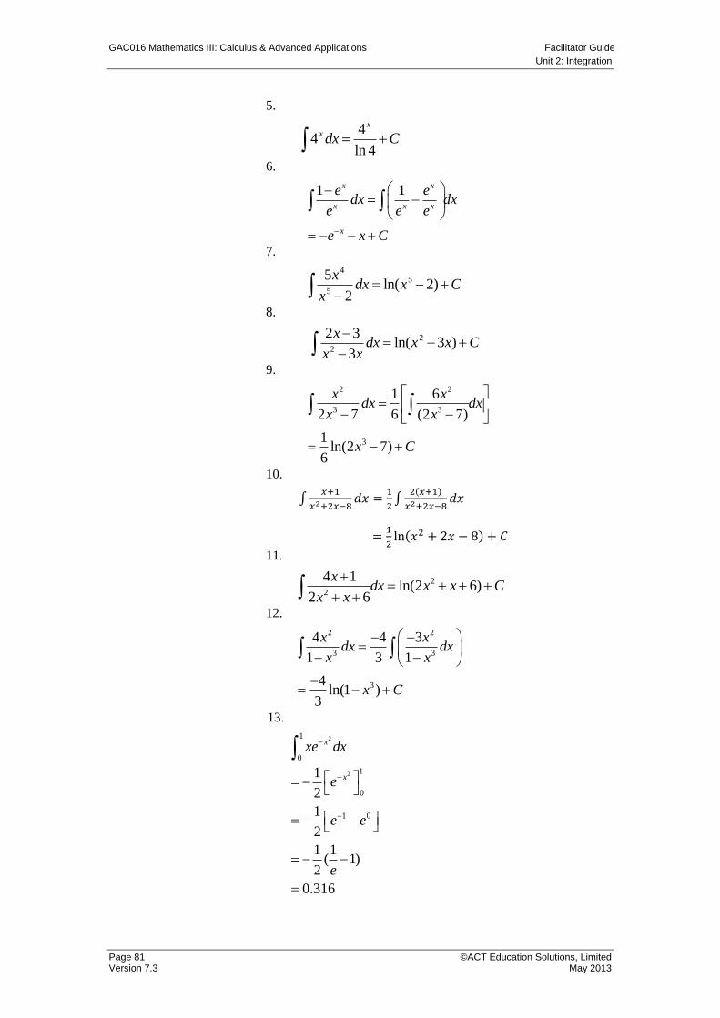
GAC016 Mathematics III: Calculus & Advanced Applications Facilitator Guide
Unit 2: Integration
Page 81 ©ACT Education Solutions, Limited Version 7.3 May 2013
5.
4
4ln 4
xx dx C
6.
1 1x x
x x x
x
e edx dx
e e e
e x C
7.
45
5
5ln( 2)
2
xdx x C
x
8.
2
2
2 3ln( 3 )
3
xdx x x C
x x
9.
2 2
3 3
3
1 6
2 7 6 (2 7)
1ln(2 7)
6
x xdx dx
x x
x C
10.
∫𝑥+1
𝑥2+2𝑥−8𝑑𝑥 =
1
2∫
2(𝑥+1)
𝑥2+2𝑥−8𝑑𝑥
=1
2ln(𝑥2 + 2𝑥 − 8) + 𝐶
11.
2
2
4 1ln(2 6)
2 6
xdx x x C
x x
12.
2 2
3 3
3
4 4 3
1 3 1
4ln(1 )
3
x xdx dx
x x
x C
13.
21
0
xxe dx
2 1
0
1 0
1
2
1
2
1 1( 1)
2
0.316
xe
e e
e
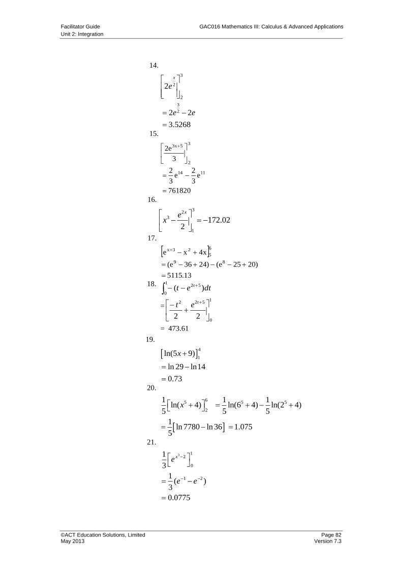
Facilitator Guide GAC016 Mathematics III: Calculus & Advanced Applications
Unit 2: Integration
©ACT Education Solutions, Limited Page 82 May 2013 Version 7.3
14.
3
2
22
x
e
3
22 2
3.5268
e e
15.
3
2
5x3
3
e2
761820
e3
2e
3
2 1114
16.
3
23
1
172.022
xex
17.
6523x x4xe
13.5115
)2025e()2436e( 89
18.
1
0
52 )( dtet t
=1
0
522
22
tet
= 473.61
19.
4
1ln(5 9)
ln 29 ln14
0.73
x
20.
65 5 5
2
1 1 1ln( 4) ln(6 4) ln(2 4)
5 5 5
1ln 7780 ln 36 1.075
5
x
21.
3 12
0
1 2
1
3
1( )
3
0.0775
xe
e e
GAC016 Mathematics III: Calculus & Advanced Applications Facilitator Guide
Unit 2: Integration
Page 83 ©ACT Education Solutions, Limited Version 7.3 May 2013
22.
2
3
1
ln( 1)3
xx
= )0ln
3
1()1ln
3
2(
3
= Undefined
23.
12
-12ln( 1)
2 ln 2 - 2 ln 2
0
x
24.
4055.0
2ln3ln
)1ln()1ln(
)1ln(
02ln
2ln
0
ee
e x
25.
4 400
sin . cos 0.293x dx x
sin cos( )n
n kx a dx kx a Ck
26.
1sin 0.00873
2
0.00873
dx dx
x
27.
cos 4 sin 4 cos 4 sin 4
1 1sin 4 cos 4
4 4
1sin 4 cos 4
4
x x dx x dx x dx
x x
x x
28.
4 4
22
cos sin
sin sin4 2
0.707 ( 1)
1.707
d
Facilitator Guide GAC016 Mathematics III: Calculus & Advanced Applications
Unit 2: Integration
©ACT Education Solutions, Limited Page 84 May 2013 Version 7.3
29.
2 2 2
0 0 0sin cos sin cos
cos cos 0 sin sin 02 2
0 1 1 0
2
d d d
30.
1 1cos 2 cos 2
2 3 2 3
1 1sin 2
2 2 3
1sin 2
4 3
x dx x dx
x C
x C
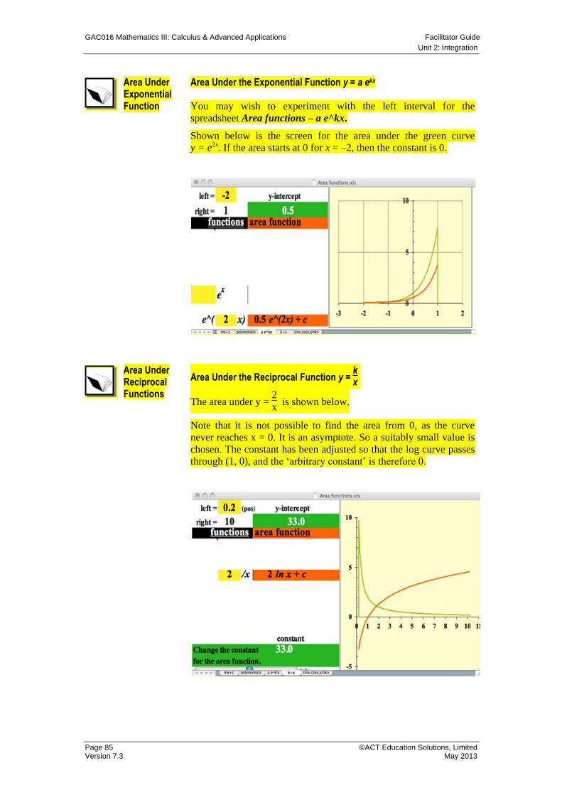
GAC016 Mathematics III: Calculus & Advanced Applications Facilitator Guide
Unit 2: Integration
Page 85 ©ACT Education Solutions, Limited Version 7.3 May 2013
Area Under Exponential Function
Area Under the Exponential Function y = a ekx
You may wish to experiment with the left interval for the
spreadsheet Area functions – a e^kx.
Shown below is the screen for the area under the green curve
y = e2x. If the area starts at 0 for x = –2, then the constant is 0.
Area Under Reciprocal Functions
Area Under the Reciprocal Function y = kx
The area under y = 2
x is shown below.
Note that it is not possible to find the area from 0, as the curve
never reaches x = 0. It is an asymptote. So a suitably small value is
chosen. The constant has been adjusted so that the log curve passes
through (1, 0), and the ‘arbitrary constant’ is therefore 0.
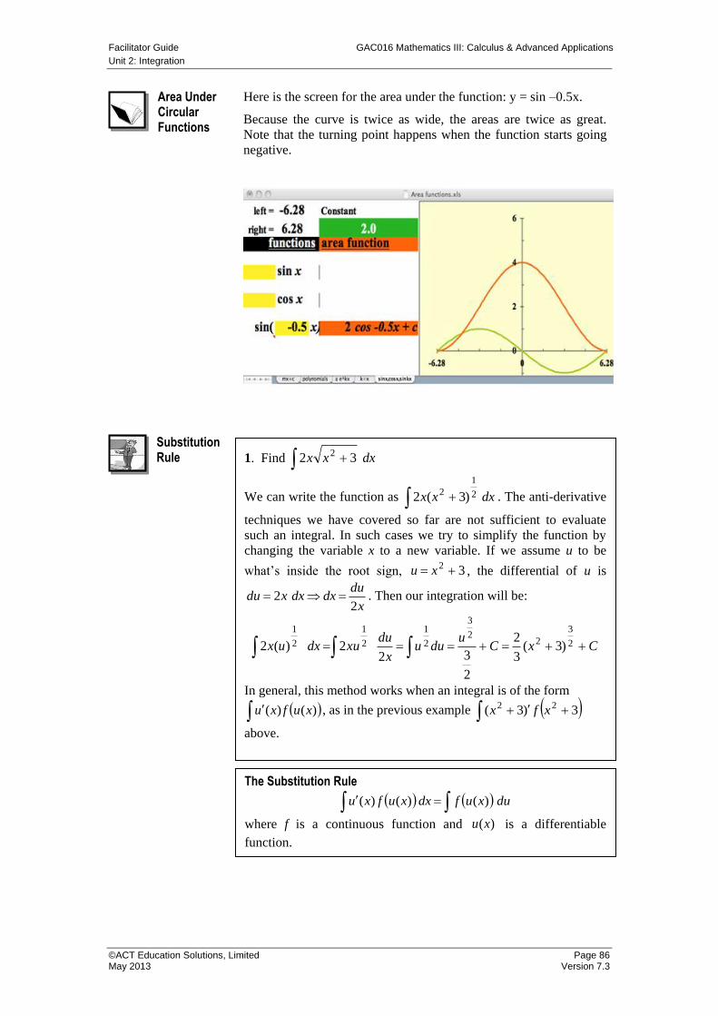
Facilitator Guide GAC016 Mathematics III: Calculus & Advanced Applications
Unit 2: Integration
©ACT Education Solutions, Limited Page 86 May 2013 Version 7.3
Area Under Circular Functions
Here is the screen for the area under the function: y = sin –0.5x.
Because the curve is twice as wide, the areas are twice as great.
Note that the turning point happens when the function starts going
negative.
Substitution Rule
1. Find dxxx 32 2
We can write the function as dxxx 2
1
2 )3(2 . The anti-derivative
techniques we have covered so far are not sufficient to evaluate
such an integral. In such cases we try to simplify the function by
changing the variable x to a new variable. If we assume u to be
what’s inside the root sign, 32 xu , the differential of u is
x
dudxdxxdu
22 . Then our integration will be:
CxCu
duux
duxudxux 2
3
22
3
2
1
2
1
2
1
)3(3
2
2
322)(2
In general, this method works when an integral is of the form
)()( xufxu , as in the previous example 3)3( 22 xfx
above.
The Substitution Rule
duxufdxxufxu )()()(
where f is a continuous function and )(xu is a differentiable
function.
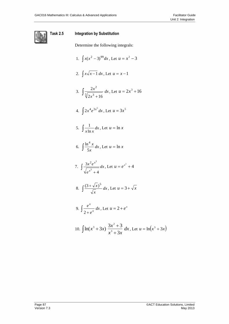
GAC016 Mathematics III: Calculus & Advanced Applications Facilitator Guide
Unit 2: Integration
Page 87 ©ACT Education Solutions, Limited Version 7.3 May 2013
Task 2.5
Integration by Substitution
Determine the following integrals:
1. dxxx 992 )3( , Let 32 xu
2. dxxx 1 , Let 1 xu
3. dx
x
x
5 3
2
162
2, Let 162 3 xu
4. dxex x
5342 , Let
53xu
5. dxxx ln
1, Let xu ln
6. dxx
x 5
ln4
, Let xu ln
7.
dx
e
ex
x
x
4
3
3
32
, Let 43
xeu
8. dxx
x
5)3(, Let xu 3
9. dxe
ex
x
2
, Let xeu 2
10. dxxx
xxx
3
33)3ln(
3
2
3, Let xxu 3ln 3
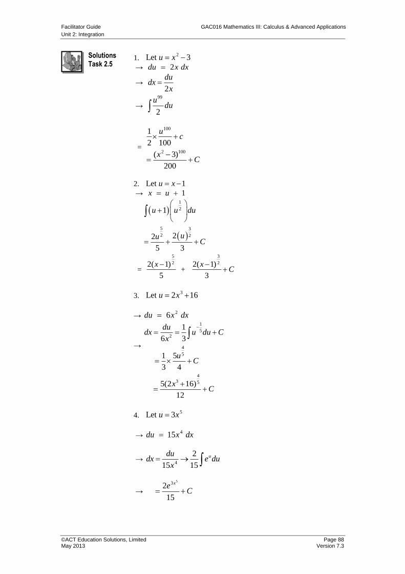
Facilitator Guide GAC016 Mathematics III: Calculus & Advanced Applications
Unit 2: Integration
©ACT Education Solutions, Limited Page 88 May 2013 Version 7.3
Solutions Task 2.5
1. 2Let 3u x
→ 2 du x dx
→ 2
dudx
x
→ duu
2
99
=
100
2 100
1
2 100
( 3)
200
uc
xC
2. Let 1u x
→ 1 x u
1
2
5 3
2 2
1
22
5 3
u u du
uuC
=
5
22( 1)
5
x +
3
22( 1)
3
xC
3. 3Let 2 16u x
→ 2 6 du x dx
→
1
52
4
5
1
6 3
1 5
3 4
dudx u du C
x
uC
4
3 55(2 16)
12
xC
4. 5Let 3u x
→ 4 15 du x dx
→ 4
2
15 15
ududx e du
x
→
532
15
xeC
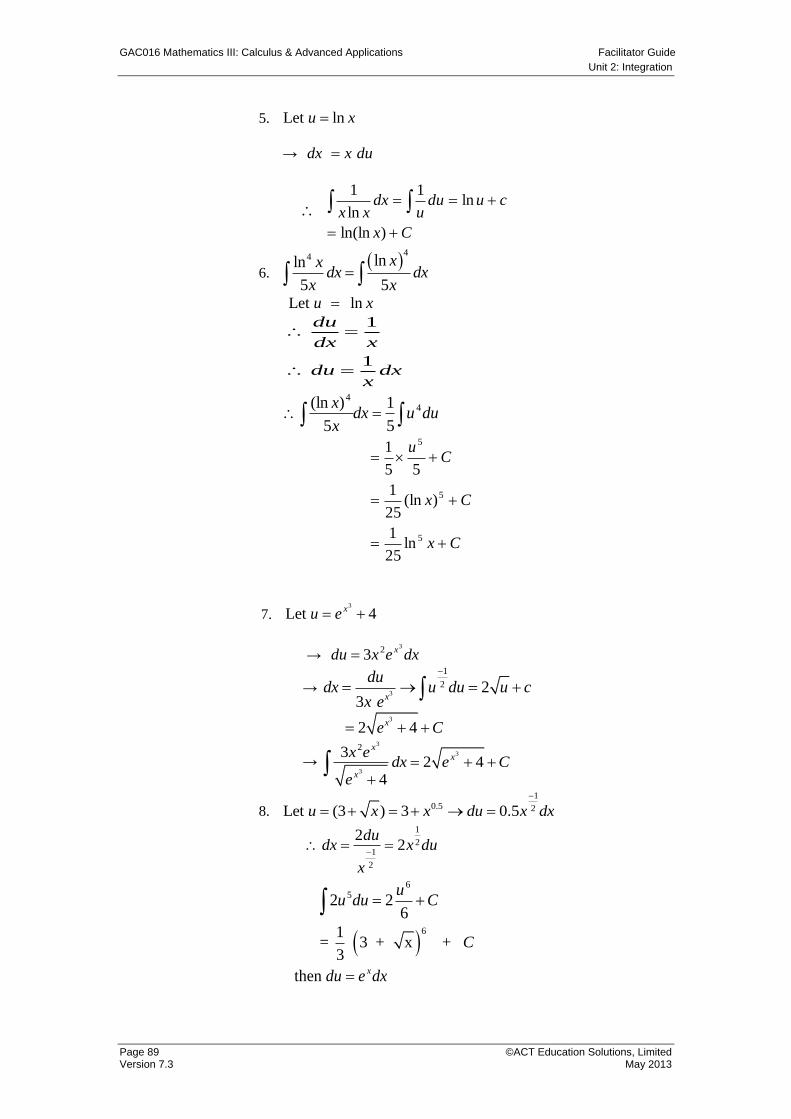
GAC016 Mathematics III: Calculus & Advanced Applications Facilitator Guide
Unit 2: Integration
Page 89 ©ACT Education Solutions, Limited Version 7.3 May 2013
5. Let lnu x
→ dx x du
Cx
cuduu
dxxx
)ln(ln
ln1
ln
1
6.
44 lnln
5 5
xxdx dx
x x
Let ln u x
1
1
du
dx x
du dxx
duudxx
x 44
5
1
5
)(ln
Cx
Cx
Cu
5
5
5
ln25
1
)(ln25
1
55
1
7. 3
Let 4xu e
→ 323 xdu x e dx
→ 3
1
2 23 x
dudx u du u c
x e
3
2 4xe C
→
3
3
3
232 4
4
xx
x
x edx e C
e
8.
1
0.5 2Let (3 ) 3 0.5u x x du x dx
1
21
2
22
dudx x du
x
652 2
6
uu du C
61
= 3 + x + 3
C
then xdu e dx
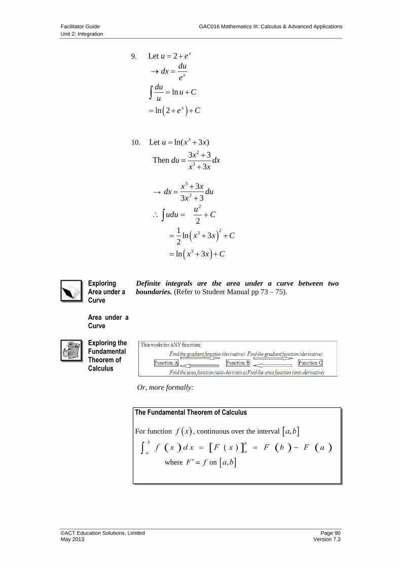
Facilitator Guide GAC016 Mathematics III: Calculus & Advanced Applications
Unit 2: Integration
©ACT Education Solutions, Limited Page 90 May 2013 Version 7.3
Exploring Area under a Curve
Area under a Curve
Definite integrals are the area under a curve between two
boundaries. (Refer to Student Manual pp 73 – 75).
Exploring the Fundamental Theorem of Calculus
Or, more formally:
9. Let 2 xu e
xe
dudx
ln
ln 2 x
duu C
u
e C
10. 3Let ln( 3 ) u x x
2
3
3 3Then
3
xdu dx
x x
→
3
2
3
3 3
x xdx du
x
udu Cu
2
2
23
3
1ln 3
2
ln 3
x x C
x x C
The Fundamental Theorem of Calculus
For function , continuous over the interval
where on
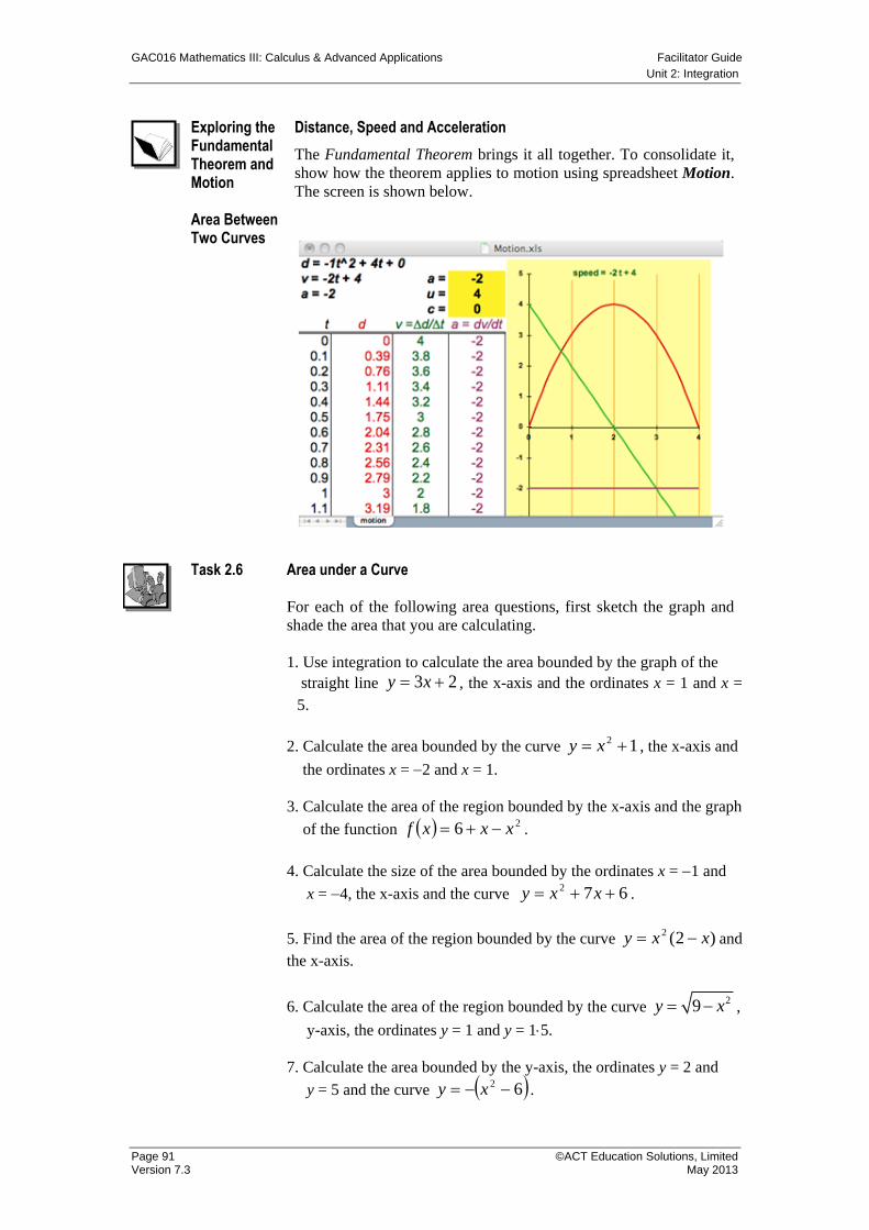
GAC016 Mathematics III: Calculus & Advanced Applications Facilitator Guide
Unit 2: Integration
Page 91 ©ACT Education Solutions, Limited Version 7.3 May 2013
Exploring the Fundamental Theorem and Motion Area Between Two Curves
Distance, Speed and Acceleration
The Fundamental Theorem brings it all together. To consolidate it,
show how the theorem applies to motion using spreadsheet Motion.
The screen is shown below.
Task 2.6 Area under a Curve
For each of the following area questions, first sketch the graph and
shade the area that you are calculating.
1. Use integration to calculate the area bounded by the graph of the
straight line 23 xy , the x-axis and the ordinates x = 1 and x =
5.
2. Calculate the area bounded by the curve 12 xy , the x-axis and
the ordinates x = 2 and x = 1.
3. Calculate the area of the region bounded by the x-axis and the graph
of the function 26 xxxf .
4. Calculate the size of the area bounded by the ordinates x = 1 and
x = 4, the x-axis and the curve 672 xxy .
5. Find the area of the region bounded by the curve )2(2 xxy and
the x-axis.
6. Calculate the area of the region bounded by the curve 29y x ,
y-axis, the ordinates y = 1 and y = 15.
7. Calculate the area bounded by the y-axis, the ordinates y = 2 and
y = 5 and the curve 62 xy .

Facilitator Guide GAC016 Mathematics III: Calculus & Advanced Applications
Unit 2: Integration
©ACT Education Solutions, Limited Page 92 May 2013 Version 7.3
8. Find the area of the region (to 2 decimal places) bounded by the
curve xey and:
a) the ordinates x = 1 and x = 3 and the x-axis.
b) the ordinates y = 1 and y = 4 and the y-axis.
9. Find the area of the shaded regions in each of the diagrams below.
a)
b) bounded by the y-axis
c)
d)
y = x + 2
y = x2
2 y = - x2 + 2
x
y
y = x
y = x3 y = x
y = 8
x
y
y = -x
y =
2
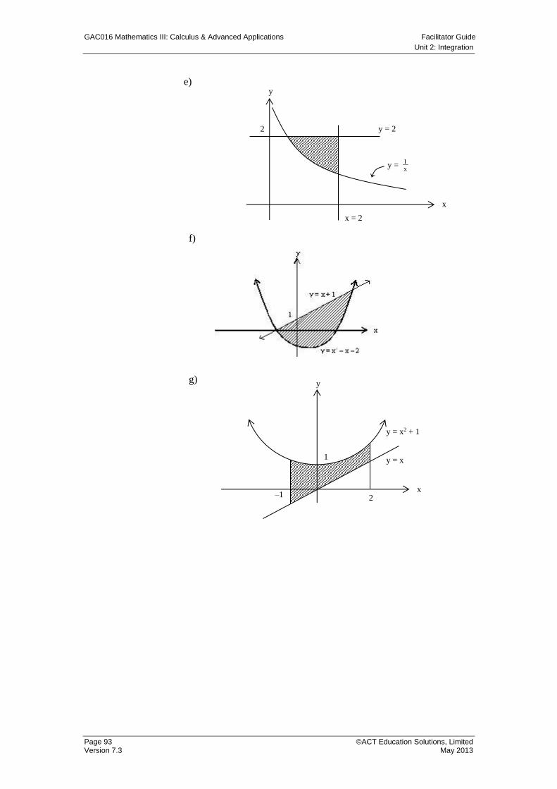
GAC016 Mathematics III: Calculus & Advanced Applications Facilitator Guide
Unit 2: Integration
Page 93 ©ACT Education Solutions, Limited Version 7.3 May 2013
e)
f)
g)
x
y
2 y = 2
x = 2
y =
x
y
y = x
y = x2 + 1
–1
1
2
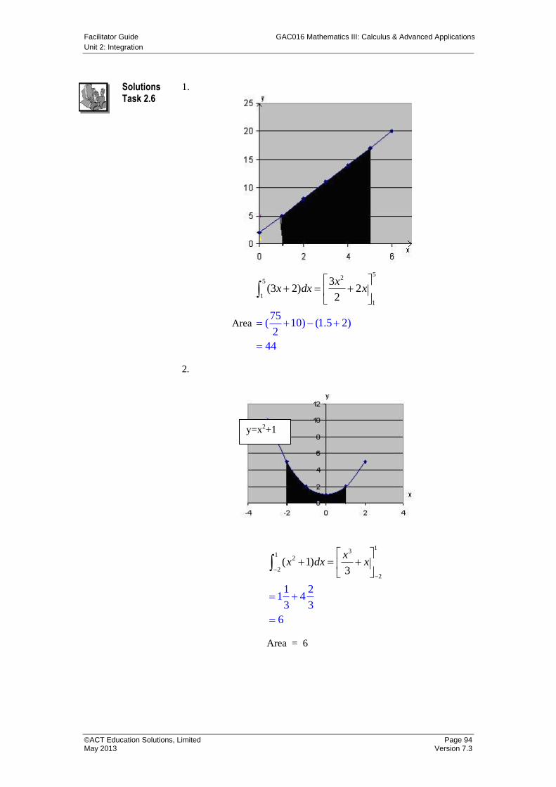
Facilitator Guide GAC016 Mathematics III: Calculus & Advanced Applications
Unit 2: Integration
©ACT Education Solutions, Limited Page 94 May 2013 Version 7.3
Solutions Task 2.6
1.
Area
52
5
11
75( 10) (1.5 2)
2
4
3(3 2) 2
2
4
xx dx x
2.
13
12
22
(
1 21 4
3 3
6
1)3
xx dx x
Area = 6
y=x2+1
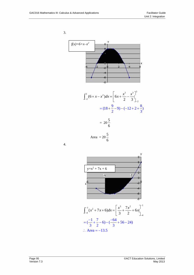
GAC016 Mathematics III: Calculus & Advanced Applications Facilitator Guide
Unit 2: Integration
Page 95 ©ACT Education Solutions, Limited Version 7.3 May 2013
3.
32 3
32
22
9 8(18 9) ( 12 2 )
2
(6 ) 6
3
2 3
x xx x dx x
= 206
5
Area = 206
5
4.
1
3 21
2
44
1 7 64( 6) ( 56 24)
3 2
7( 7 6) 6
3 2
3
Area 13.5
x xx x dx x
f(x)=6+x–x2
y=x2 + 7x + 6
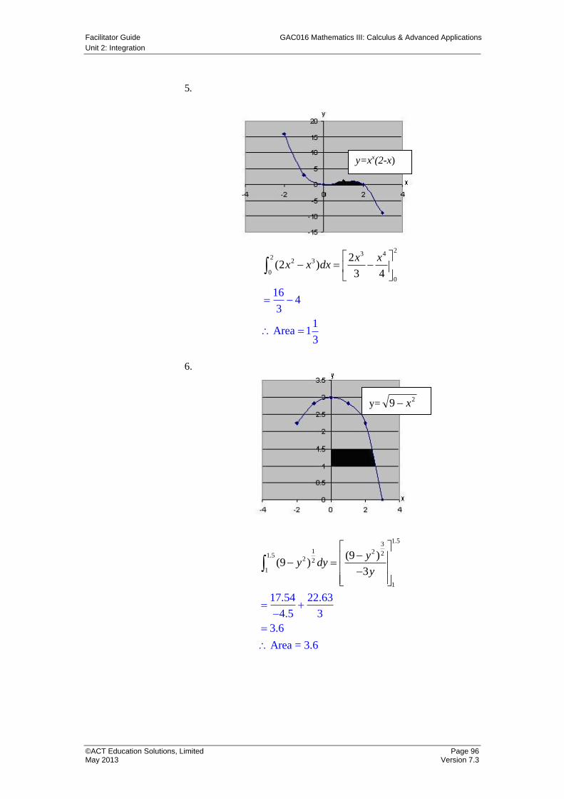
Facilitator Guide GAC016 Mathematics III: Calculus & Advanced Applications
Unit 2: Integration
©ACT Education Solutions, Limited Page 96 May 2013 Version 7.3
5.
2
3 42
2 3
00
2(2 )
3
164
3
1Area 1
3
4
x xx x dx
6.
1.53
1 2 21.52 2
1
1
17.54 22
(9 )(
.63
4.5 3
3.6
Are
9 )
a 3.
3
= 6
yy dy
y
y=xx(2-x)
y=29 x
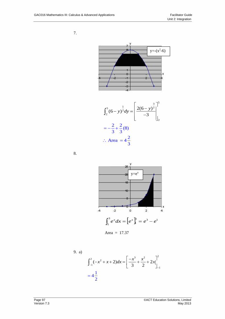
GAC016 Mathematics III: Calculus & Advanced Applications Facilitator Guide
Unit 2: Integration
Page 97 ©ACT Education Solutions, Limited Version 7.3 May 2013
7.
53
1 252
2
2
2(6 )(6 )
3
2 2(8)
3 3
2Area 4
3
yy dy
8.
3
1
133
1 eeedxe xx
Area = 17.37
9. a) 2
3 22
2
11
( 2) 23 2
14
2
x xx x dx x
y=-(x2-6)
y=ex
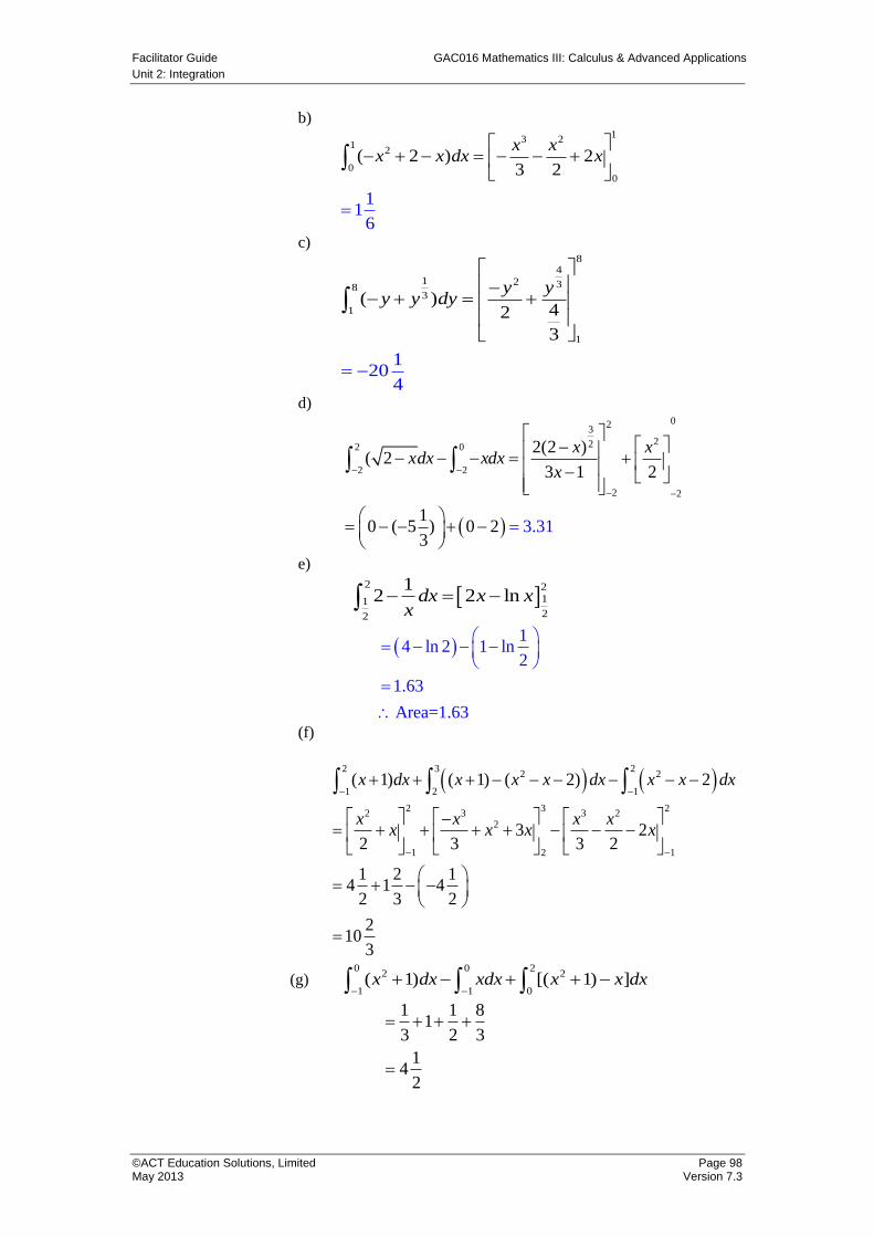
Facilitator Guide GAC016 Mathematics III: Calculus & Advanced Applications
Unit 2: Integration
©ACT Education Solutions, Limited Page 98 May 2013 Version 7.3
b) 1
3 21
2
00
( 2 ) 23 2
11
6
x xx x dx x
c) 8
41 2 383
1
1
( )42
3
120
4
y yy y dy
d)
023
222 0
2 2
2 2
2(2 )( 2
3
3
1 2
10 ( 5 ) 0 2 .31
3
x xxdx xdx
x
e)
2 2
11
22
12 2 lndx x x
x
1
4 ln 2 1 ln2
1.63
Area=1.63
(f)
2 3 2
2 2
1 2 1
2 3 22 3 3 2
2
1 2 1
( 1) ( 1) ( 2) 2
3 22 3 3 2
1 2 14 1 4
2 3 2
210
3
x dx x x x dx x x dx
x x x xx x x x
(g) 0 0 2
2 2
1 1 0( 1) [( 1) ]x dx xdx x x dx
1 1 81
3 2 3
14
2

GAC016 Mathematics III: Calculus & Advanced Applications Facilitator Guide
Unit 2: Integration
Page 99 ©ACT Education Solutions, Limited Version 7.3 May 2013
Part E The Volume of Rotation
Refer to Student Manual (pp 85 – 87).
Task 2.7 Volumes of Rotation
1. Find the volume formed by rotating the curve 𝑦 = 𝑥3 between x =
0 and x = 2 around the x-axis.
2. Calculate the volume formed when the curve 𝑦 = 𝑥2 + 1 between x
= 0 and x = 2 is rotated around the y-axis.
3. Find the volume created when the area bounded by the curve 𝑦 =
4 − 𝑥2 and the x-axis is rotated around:
(a) the x-axis.
(b) the y-axis.
4. Calculate the volume of revolution resulting from rotating the curve
𝑦 = 𝑒−𝑥 between x = 0 and x = 1 around the x-axis.
5. Find the volume formed from rotating the curve 𝑦 = √𝑥2(𝑥2 + 1)4
between x = 0 and x = 3 around the x-axis.
Solutions for Task 2.7
1. 𝑉 = 𝜋 ∫ 𝑥6𝑑𝑥2
0= 𝜋 [
1
7𝑥7]
0
2=
128
7𝜋
2. 𝑉 = 𝜋 ∫ (√𝑦 − 1)2
𝑑𝑦5
1= 𝜋 [
1
2𝑦2 − 𝑦]
1
5= 8𝜋
3. (a) 𝑉 = 𝜋 ∫ (4 − 𝑥2)2𝑑𝑥2
−2= 𝜋 [16𝑥 −
8
3𝑥3 +
1
5𝑥5]
−2
2=
512
15𝜋
(b) 𝑉 = 𝜋 ∫ (√4 − 𝑦)2
𝑑𝑦4
0= 𝜋 [4𝑦 −
1
2𝑦2]
0
4= 8𝜋
4. 𝑉 = 𝜋 ∫ 𝑒−2𝑥𝑑𝑥1
0= 𝜋 [−
1
2𝑒−2𝑥]
0
1=
𝜋
2(1 − 𝑒−2)
5. 𝑉 = 𝜋 ∫ 𝑥√𝑥2 + 1𝑑𝑥3
0
= 𝜋 ∙1
2∫ √𝑢𝑑𝑢
10
1 (Substituting 𝑢 = 𝑥2 + 1)
=𝜋
2[
2
3𝑢
3
2]1
10
=𝜋
3(10√10 − 1)
Facilitator Guide GAC016 Mathematics III: Calculus & Advanced Applications
Unit 2: Integration
©ACT Education Solutions, Limited Page 100 May 2013 Version 7.3
Assessment Event 1
The In-class Test should be administered at the end of Unit 2. Note that
this is an in-class test conducted under test conditions.
Assessment Event 4
Collect the Mathematical Terminology Logbooks from students for
marking.
GAC016 Mathematics III: Calculus & Advanced Applications Facilitator Guide
Unit 3: Advanced Applications
Page 101 ©ACT Education Solutions, Limited Version 7.3 May 2013
Unit 3: Advanced Applications
Part A Unit Introduction
Part B Terminology Introduced
Part C Motion in a Straight Line (Rectilinear Motion)
Part D Approximation Methods in Integration
Part E Problems involving Maxima and Minima
Part F Exponential Growth and Decay
Part G Verhulst-Pearl Logistic Function – The Natural Law of Growth and
Decay
Part A Unit Introduction
Overview In this unit, students will learn to apply differentiation and
integration techniques to solve a variety of problems.
In this unit, students will learn to:
apply their knowledge of calculus to a variety of practical
situations;
learn some applications of differentiation and integration
using techniques learnt in the previous two units
learn how to solve different problems that involve
maximising or minimising a quantity.
This unit includes a series of tasks that students will work through
to practise the course material. They will be expected to complete
some work in their own time. You will guide them through the
unit.
Assessment
Events 2, 3
and 4
Project 2 to be undertaken by students following completion of
Part C – Motion in a Straight Line – Rectilinear Motion – in this
Unit.
The Examination is to be conducted at the end of Unit 3.
Students are also required to submit their Mathematical
Terminology Logbooks at the end of Unit 3.
Remind students of assessment due dates and requirements.
Facilitator Guide GAC016 Mathematics III: Calculus & Advanced Applications
Unit 3: Advanced Applications
©ACT Education Solutions, Limited Page 102 May 2013 Version 7.3
Part B Terminology Introduced
By the end of this unit, students need to know the meanings of these
terms. The terms are bolded in the first instance they occur. Please
make sure students understand the definitions of new terminology
and include these words in their Mathematical Terminology
Logbook.
Summary of Terms
averages
marginal
total cost
revenue
demand function
variation
quantity
marginal revenue
marginal cost
trapezoidal rule
Simpson’s rule
numerical method
marginal revenue product
consumer’s surplus
producer’s surplus
equilibrium point
logistic function
Verhulst-Pearl logistic
maximising
disease
minimising
subintervals
approximation
intervals
GAC016 Mathematics III: Calculus & Advanced Applications Facilitator Guide
Unit 3: Advanced Applications
Page 103 ©ACT Education Solutions, Limited Version 7.3 May 2013
Part C Motion in a Straight Line (Rectilinear Motion)
Motion in a Straight Line
Important
Integration in Motion Equations
Task 3.1
Refer to Student Manual (pp. 91).
Important Terms to Know for This Topic:
i) INITIALLY: At the Beginning (t = 0)
ii) AT REST: Velocity = 0 (V = 0)
iii) AT THE ORIGIN: Displacement = 0 ( 0S )
Note: ‘S’ does not measure the distance travelled but measures how far the
particle is from the origin, ‘S’ measures displacement.
Since the acceleration is the derivative of the velocity and the velocity
is the derivative of the displacement therefore velocity is the
Primitive Function of acceleration and displacement is the Primitive
Function of velocity.
if )(tfa
adtV
1. The equation for displacement of a particle is given by
3104 2 ttS
i) Find its initial velocity and acceleration.
ii) Find when the particle is at rest
iii) Find the displacement and acceleration after 4
seconds.
2. The equation for displacement of a particle is given by
32 teS
i) Find the initial velocity
ii) Find the acceleration after 2 seconds
iii) Show that the acceleration is always double the
velocity
3. The acceleration of a particle is given by 12sin 2a t if
initially the particle is at rest at the origin find the exact
displacement after 4
seconds.
4. The velocity of a particle is given by2 4
tv
t
if the particle
is initially at the origin find the displacement after 4 seconds.
Note: Do NOT forget the constant
when finding these Primitive
Functions
Facilitator Guide GAC016 Mathematics III: Calculus & Advanced Applications
Unit 3: Advanced Applications
©ACT Education Solutions, Limited Page 104 May 2013 Version 7.3
Solutions Task 3.1
1. 3104 2 ttS
8
108
a
tV
(i.) initial velocity (t = 0) = sm /10
initial acceleration = 82/ sm
(ii.) at rest: 0V
4
11
0108
t
t
(iii.) 4t , 3)4(10)4(4 2 S
m27 2/8 sma
2. 32 teS
t
t
ea
eV
2
2
4
2
(i.) Initial velocity (t = 0) = sme /22 0
(ii.) When t = 2, 𝑎 = 4𝑒4
(iii.) tea 24
Va
eV t
2
2 2
3. ta 2sin12
CtV
2cos
2
112
Ct 2cos6
When 0t , 0V
CttS
tV
C
C
62sin3
62cos6
6
0cos60
0t , 0S
ttS
C
C
62sin3
0
000
When 4
t ,
46
2sin3
S
2
33
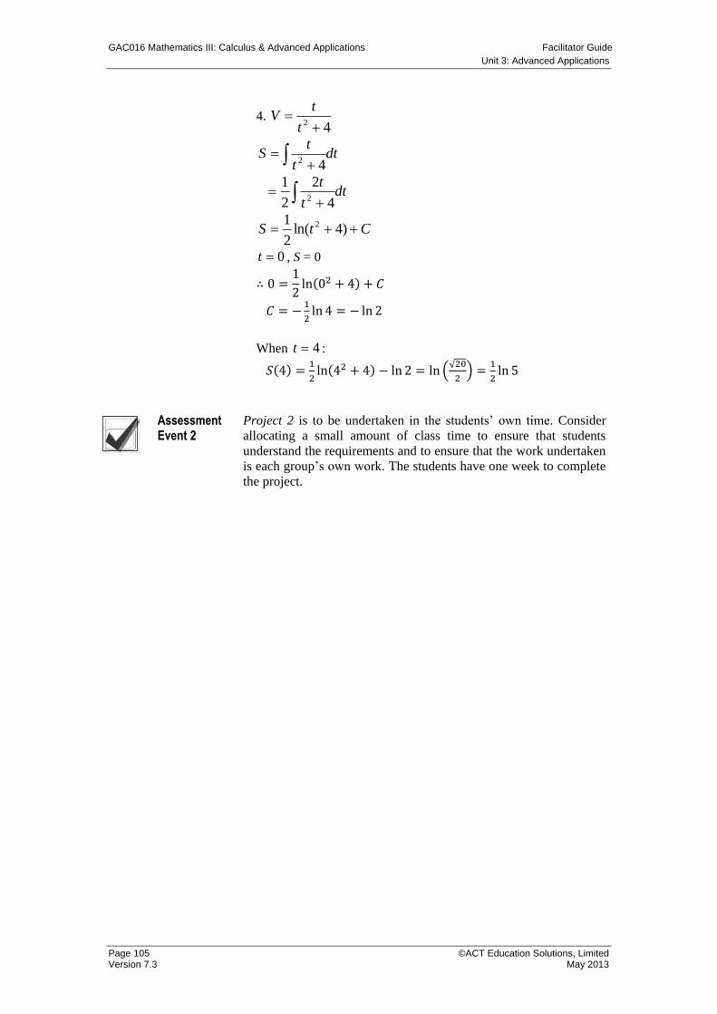
GAC016 Mathematics III: Calculus & Advanced Applications Facilitator Guide
Unit 3: Advanced Applications
Page 105 ©ACT Education Solutions, Limited Version 7.3 May 2013
4. 42
t
tV
dtt
tS
42
dtt
t
4
2
2
12
CtS )4ln(2
1 2
0t , S = 0
∴ 0 =1
2ln(02 + 4) + 𝐶
𝐶 = −1
2ln 4 = − ln 2
When 4t :
𝑆(4) =1
2ln(42 + 4) − ln 2 = ln ቀ
√20
2ቁ =
1
2ln 5
Assessment Event 2
Project 2 is to be undertaken in the students’ own time. Consider
allocating a small amount of class time to ensure that students
understand the requirements and to ensure that the work undertaken
is each group’s own work. The students have one week to complete
the project.
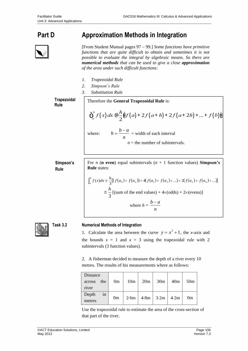
Facilitator Guide GAC016 Mathematics III: Calculus & Advanced Applications
Unit 3: Advanced Applications
©ACT Education Solutions, Limited Page 106 May 2013 Version 7.3
Part D Approximation Methods in Integration
Trapezoidal Rule Simpson’s
Rule
[From Student Manual pages 97 – 99.] Some functions have primitive
functions that are quite difficult to obtain and sometimes it is not
possible to evaluate the integral by algebraic means. So there are
numerical methods that can be used to give a close approximation
of the area under such difficult functions:
1. Trapezoidal Rule
2. Simpson’s Rule
3. Substitution Rule
Task 3.2 Numerical Methods of Integration
1. Calculate the area between the curve 13 xy , the x-axis and
the bounds x = 1 and x = 3 using the trapezoidal rule with 2
subintervals (3 function values).
2. A fisherman decided to measure the depth of a river every 10
metres. The results of his measurements where as follows:
Use the trapezoidal rule to estimate the area of the cross-section of
that part of the river.
Distance
across the
river
0m
10m
20m
30m
40m
50m
Depth in
metres 0m 26m 48m 32m 42m 0m
Therefore the General Trapezoidal Rule is:
f x( )dxa
b
ò @h
2f a( ) + 2 f a+h( ) +2 f a+ 2h( ) +...+ f b( )éë ùû
where: n
abh
= width of each interval
n = the number of subintervals.
For n (n even) equal subintervals (n + 1 function values) Simpson’s
Rule states:
b
an afafafafafaf
hdxxf ...2...4
3)( 42310
3
h [(sum of the end values) + 4(odds) + 2(evens)]
where h = n
ab
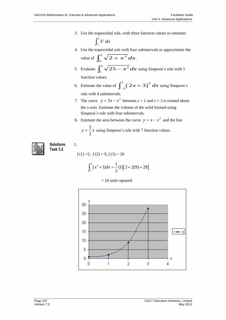
GAC016 Mathematics III: Calculus & Advanced Applications Facilitator Guide
Unit 3: Advanced Applications
Page 107 ©ACT Education Solutions, Limited Version 7.3 May 2013
3. Use the trapezoidal rule, with three function values to estimate:
5
33 dxx
4. Use the trapezoidal rule with four subintervals to approximate the
value of 2
0
22 dxx .
5. Evaluate 5
1
225 dxx using Simpson’s rule with 5
function values.
6. Estimate the value of 1 4
32 3x dx
using Simpson’s
rule with 4 subintervals.
7. The curve 23 xxy between x = 1 and x = 3 is rotated about
the x-axis. Estimate the volume of the solid formed using
Simpson’s rule with four subintervals.
8. Estimate the area between the curve 2xxy and the line
xy2
5 using Simpson’s rule with 7 function values.
Solutions Task 3.2
1.
f (1) =2, f (2) = 9, f (3) = 28
3
3
1
1( 1) (1) 2 2(9) 28
2x dx
= 24 units squared
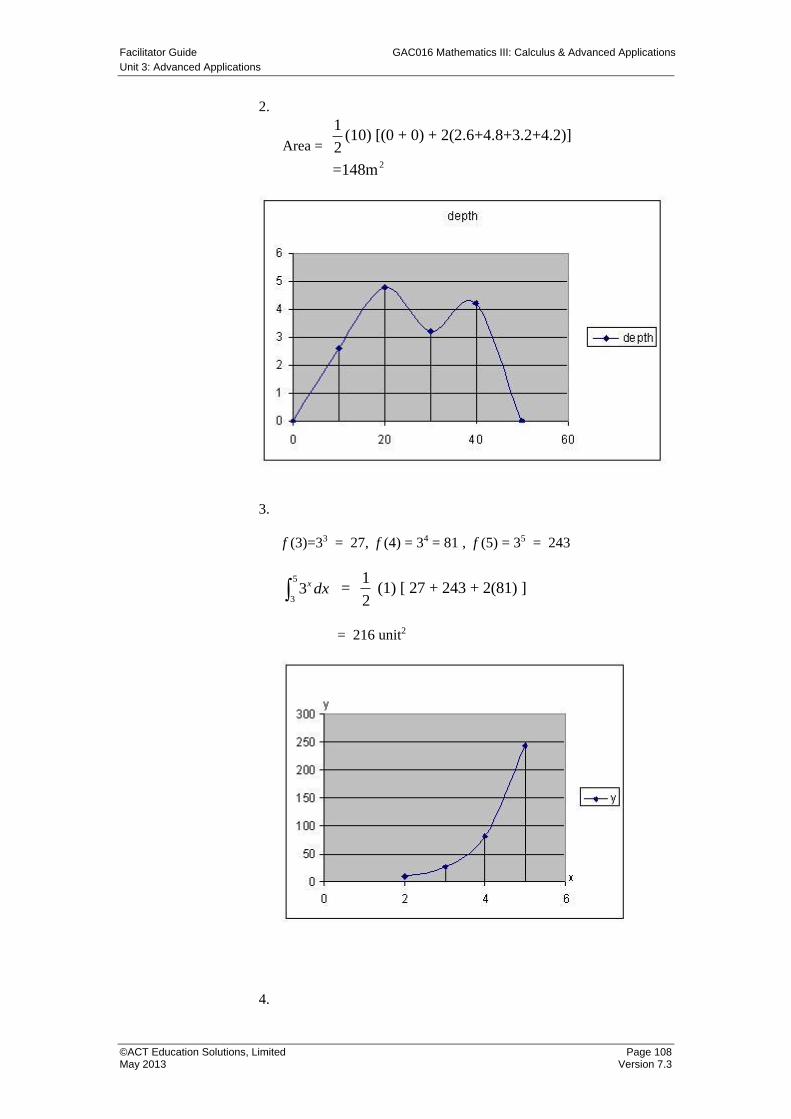
Facilitator Guide GAC016 Mathematics III: Calculus & Advanced Applications
Unit 3: Advanced Applications
©ACT Education Solutions, Limited Page 108 May 2013 Version 7.3
2.
Area =
2
1(10) [(0 + 0) + 2(2.6+4.8+3.2+4.2)]
2
=148m
3.
f (3)=33 = 27, f (4) = 34 = 81 , f (5) = 35 = 243
5
33 dxx
1
= (1) [ 27 + 243 + 2(81) ] 2
= 216 unit2
4.
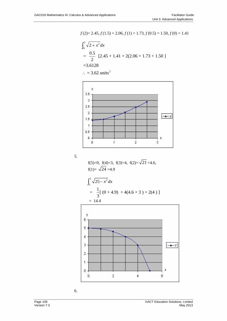
GAC016 Mathematics III: Calculus & Advanced Applications Facilitator Guide
Unit 3: Advanced Applications
Page 109 ©ACT Education Solutions, Limited Version 7.3 May 2013
f (2)= 2.45, f (1.5) = 2.06, f (1) = 1.73, f (0.5) = 1.50, f (0) = 1.41
2
0
22 dxx
2
0.5= [2.45 + 1.41 + 2(2.06 + 1.73 + 1.50 ]
2
=3.6128
= 3.62 units
5.
f(5)=0, f(4)=3, f(3)=4, f(2)= 21 =4.6,
f(1)= 24 =4.9
5
2
125 x dx
1
= [ (0 + 4.9) + 4(4.6 + 3 ) + 2(4 ) ] 3
= 14.4
6.
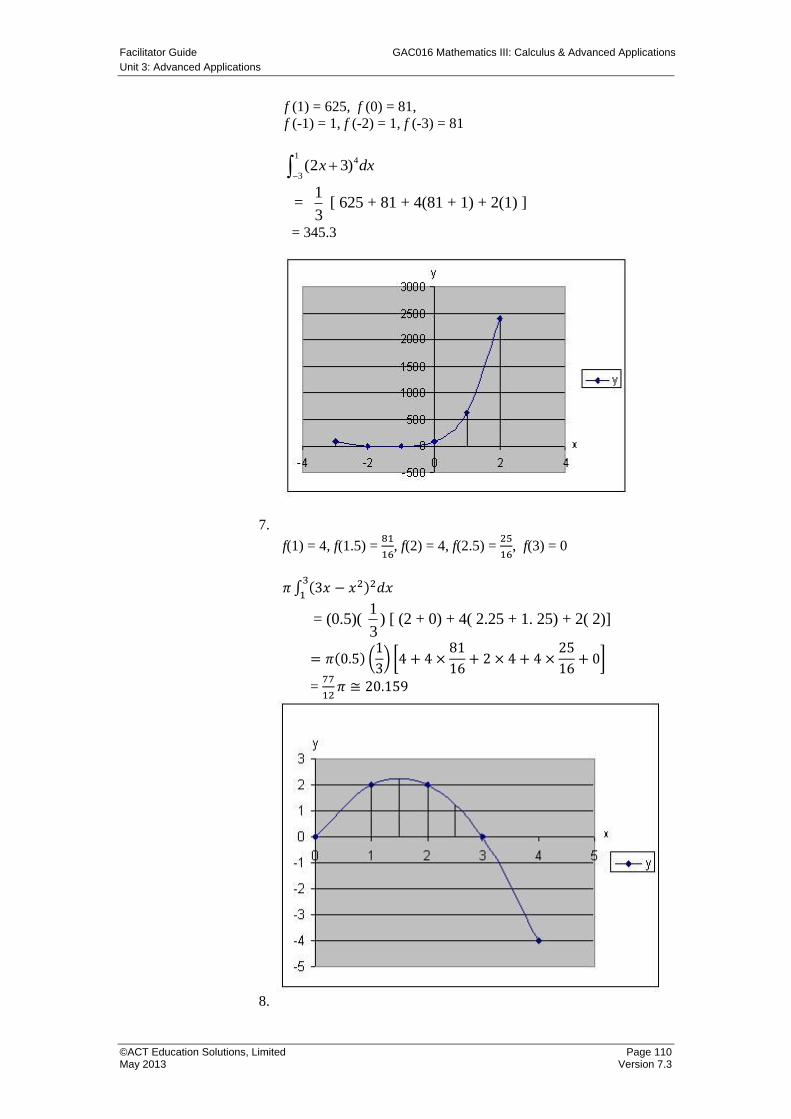
Facilitator Guide GAC016 Mathematics III: Calculus & Advanced Applications
Unit 3: Advanced Applications
©ACT Education Solutions, Limited Page 110 May 2013 Version 7.3
f (1) = 625, f (0) = 81,
f (-1) = 1, f (-2) = 1, f (-3) = 81
1
4
3(2 3)x dx
1
= [ 625 + 81 + 4(81 + 1) + 2(1) ]3
= 345.3
7.
f(1) = 4, f(1.5) = 81
16, f(2) = 4, f(2.5) =
25
16, f(3) = 0
𝜋 ∫ (3𝑥 − 𝑥2)2𝑑𝑥3
1
1 = (0.5)( ) [ (2 + 0) + 4( 2.25 + 1. 25) + 2( 2)]
3
= 𝜋(0.5) (1
3) [4 + 4 ×
81
16+ 2 × 4 + 4 ×
25
16+ 0]
= 77
12𝜋 ≅ 20.159
8.

GAC016 Mathematics III: Calculus & Advanced Applications Facilitator Guide
Unit 3: Advanced Applications
Page 111 ©ACT Education Solutions, Limited Version 7.3 May 2013
Solve y = x – x2 and y = x2
5
and obtain x = 0 or x = -1.5.
0
5.1
2 )]()2
5[( dxxxx gives the required area.
0
5.1
2 ]5.1[ dxxx
f (0)= 0, f (-0.25) = -0.3125, f (-0.5) = -0.5, f (-0.75) = -
0.5625, f (-1) = -0.5, f (-1.25) = -0.3125, f (-1.5) = 0
0
5.1
2 ]5.1[ dxxx
= 3
25.0 [ 0+0+4(-0.3125 + -0.5625 + -0.3125) + 2( -0.5 +-0.5)]
1
(0.25) (-6.75) - 0.56253
Facilitator Guide GAC016 Mathematics III: Calculus & Advanced Applications
Unit 3: Advanced Applications
©ACT Education Solutions, Limited Page 112 May 2013 Version 7.3
Part E Problems involving Maxima and Minima
Examples Involving Minima and Maxima Problems Steps in Solving Applied Maximum and Minimum Problems
Refer to Student Manual (pp 103 – 104).
Task 3.3 Maxima and Minima Problems
1. Find the two numbers whose sum is 50 and whose product is
maximum.
2. A manufacturer knows that the total cost c of producing q units is
given by 800404.0 2 qqc . Find the value of q which
minimises the average cost.
3. Suppose the demand function for a certain product is
qp 4200 , where p is the price (in dollars) per unit (q) and the
average cost function (in dollars) is q
c200
2 . Find the value
of q which maximises the profit?
4. A hotel has 80 rooms that can be rented for $400 per month.
However, for each $20 per month increase, there will be two
vacancies with no possibilities of filling them. What rent per
room will maximise the monthly revenue?
5. Find the maximum area of a rectangular that can be inscribed in a
circle of radius 8.
6. A rectangle of cardboard is 16 cm by 8 cm. In order to form a box
without a cover, identical small squares are cut from each corner
and the remaining cardboard section is folded. Find the
dimensions of the box that maximises the volume and find that
volume.
7. A power station is on one side of a river, which is 2 km away
from the beach and a house is 4 km downstream on the other side
of the river. It costs $4 per metre to run the power line on the land
and $8 per metre to run it water. How we should connect the
power lines to minimise the cost?
8. The demand function for a product is qp 4150 and the
average cost function is q
c100
8 , where q is number of units,
and both p and c are expressed in dollars per unit.
a. Determine the level of output at which profit is maximised.
b. Determine the price at which maximum profit occurs.
c. Determine the maximum profit.
d. If, as a regulatory device, the government imposes a tax of
$16 per unit on the monopolist, what is the new price for
profit maximisation?
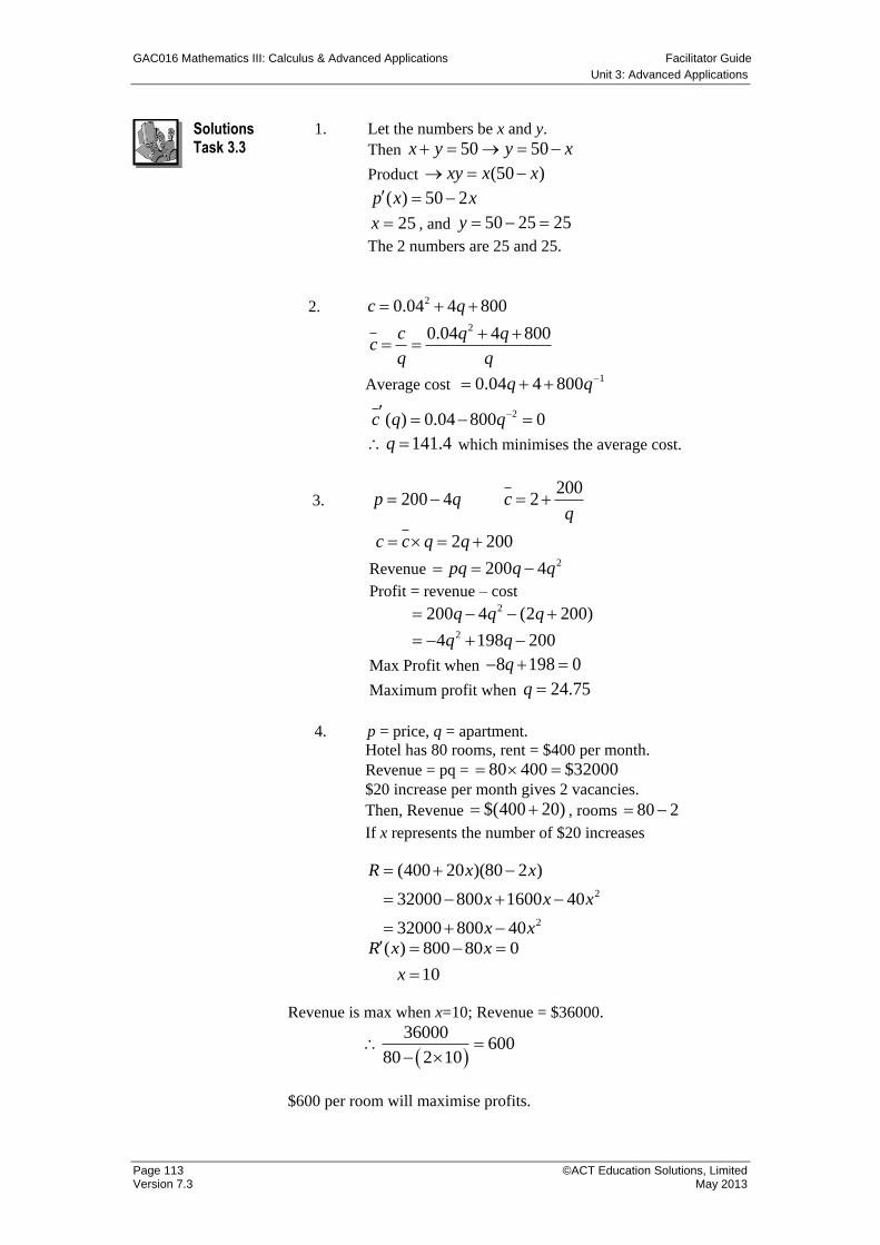
GAC016 Mathematics III: Calculus & Advanced Applications Facilitator Guide
Unit 3: Advanced Applications
Page 113 ©ACT Education Solutions, Limited Version 7.3 May 2013
Solutions Task 3.3
1. Let the numbers be x and y.
Then 50 50x y y x
Product (50 )xy x x
( ) 50 2p x x
25x , and 50 25 25y
The 2 numbers are 25 and 25.
2.
20.04 4 800c q
20.04 4 800c q qc
q q
Average cost 10.04 4 800q q
2( ) 0.04 800 0c q q
141.4q which minimises the average cost.
3. 200 4p q 200
2cq
2 200c c q q
Revenue 2200 4pq q q
Profit = revenue – cost
2200 4 (2 200)q q q
24 198 200q q
Max Profit when 8 198 0q
Maximum profit when 24.75q
4. p = price, q = apartment.
Hotel has 80 rooms, rent = $400 per month.
Revenue = pq = 80 400 $32000
$20 increase per month gives 2 vacancies.
Then, Revenue $(400 20) , rooms 80 2
If x represents the number of $20 increases
2
2
(400 20 )(80 2 )
32000 800 1600 40
32000 800 40
R x x
x x x
x x
( ) 800 80 0
10
R x x
x
Revenue is max when x=10; Revenue = $36000.
36000600
80 2 10
$600 per room will maximise profits.
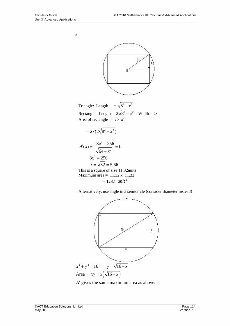
Facilitator Guide GAC016 Mathematics III: Calculus & Advanced Applications
Unit 3: Advanced Applications
©ACT Education Solutions, Limited Page 114 May 2013 Version 7.3
5.
Triangle: Length = 2 28 x
Rectangle : Length = 2 22 8 x Width = 2x
Area of rectangle = l w
2 22 (2 8 )x x
2
2
8 256( ) 0
64
xA x
x
28 256x
32 5.66x
This is a square of size 11.32units
Maximum area = 11.32 x 11.32
= 128.1 2unit
Alternatively, use angle in a semicircle (consider diameter instead)
2 2 16 16x y y x
Area 16
A gives the same maximum area as above.
xy x x
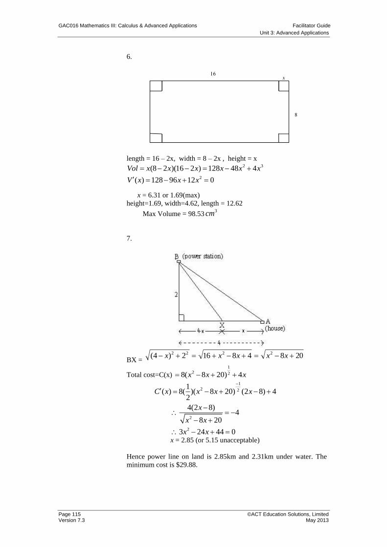
GAC016 Mathematics III: Calculus & Advanced Applications Facilitator Guide
Unit 3: Advanced Applications
Page 115 ©ACT Education Solutions, Limited Version 7.3 May 2013
6.
length = 16 – 2x, width = 8 – 2x , height = x
2 3(8 2 )(16 2 ) 128 48 4Vol x x x x x x
2( ) 128 96 12 0V x x x
x = 6.31 or 1.69(max)
height=1.69, width=4.62, length = 12.62
Max Volume = 98.533cm
7.
BX =
Total cost=C(x)
1
2 28( 8 20) 4x x x
1
2 2
2
2
1( ) 8( )( 8 20) (2 8) 4
2
4(2 8)4
8 20
3 24 44 0
C x x x x
x
x x
x x
x = 2.85 (or 5.15 unacceptable)
Hence power line on land is 2.85km and 2.31km under water. The
minimum cost is $29.88.
20848162)4( 2222 xxxxx
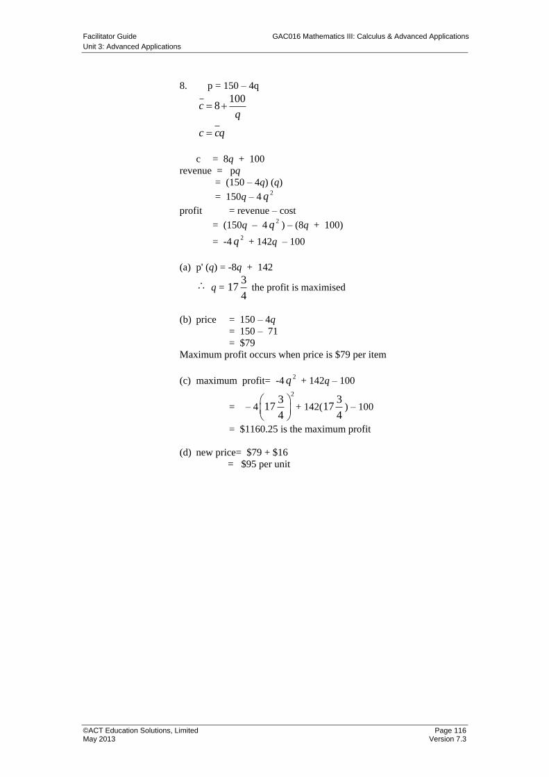
Facilitator Guide GAC016 Mathematics III: Calculus & Advanced Applications
Unit 3: Advanced Applications
©ACT Education Solutions, Limited Page 116 May 2013 Version 7.3
8. p = 150 – 4q
1008c
q
c cq
c = 8q + 100
revenue = pq
= (150 – 4q) (q)
= 150q – 42q
profit = revenue – cost
= (150q – 42q ) – (8q + 100)
= -42q + 142q – 100
(a) p' (q) = -8q + 142
q = 3
174
the profit is maximised
(b) price = 150 – 4q
= 150 – 71
= $79
Maximum profit occurs when price is $79 per item
(c) maximum profit= -42q + 142q – 100
= – 4
23
174
+ 142(3
174
) – 100
= $1160.25 is the maximum profit
(d) new price= $79 + $16
= $95 per unit
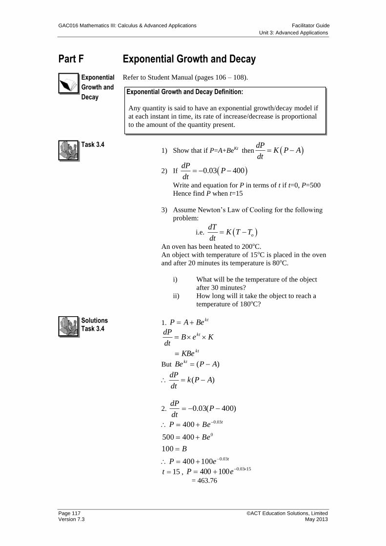
GAC016 Mathematics III: Calculus & Advanced Applications Facilitator Guide
Unit 3: Advanced Applications
Page 117 ©ACT Education Solutions, Limited Version 7.3 May 2013
Part F Exponential Growth and Decay
Exponential
Growth and
Decay
Refer to Student Manual (pages 106 – 108).
Task 3.4 1) Show that if P=A+BeKt then
dPK P A
dt
2) If 0.03 400dP
Pdt
Write and equation for P in terms of t if t=0, P=500
Hence find P when t=15
3) Assume Newton’s Law of Cooling for the following
problem:
i.e. o
dTK T T
dt
An oven has been heated to 200oC.
An object with temperature of 15oC is placed in the oven
and after 20 minutes its temperature is 80oC.
i) What will be the temperature of the object
after 30 minutes?
ii) How long will it take the object to reach a
temperature of 180oC?
Solutions Task 3.4
1. ktBeAP
KeBdt
dP kt
ktKBe
But )( APBe kt
)( APkdt
dP
2. )400(03.0 Pdt
dP
t
t
eP
B
Be
BeP
03.0
0
03.0
100400
100
400500
400
15t , 1503.0100400 eP
= 463.76
Exponential Growth and Decay Definition:
Any quantity is said to have an exponential growth/decay model if
at each instant in time, its rate of increase/decrease is proportional
to the amount of the quantity present.
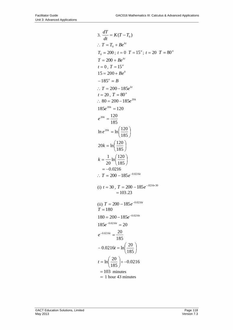
Facilitator Guide GAC016 Mathematics III: Calculus & Advanced Applications
Unit 3: Advanced Applications
©ACT Education Solutions, Limited Page 118 May 2013 Version 7.3
3. )( 0TTKdt
dT
ktBeTT 0
2000 T ; 0t oT 15 ; 20t
oT 80
ktBeT 200
0t , oT 15
kt
o
eT
B
Be
185200
185
20015 0
20t , oT 80
185
120ln
20
1
185
120ln20
185
120lnln
185
120
120185
18520080
20
20
20
20
k
k
e
e
e
e
k
k
k
k
0216.0 teT 0216.0185200
(i) 30t , 300216.185200 eT
23.103
(ii) teT 0216.0185200
0216.0185
20ln
185
20ln0216.0
185
20
20185
185200180
180
0216.0
0216.0
0216.0
t
t
e
e
e
T
t
t
t
103 minutes
1 hour 43 minutes
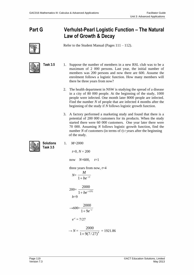
GAC016 Mathematics III: Calculus & Advanced Applications Facilitator Guide
Unit 3: Advanced Applications
Page 119 ©ACT Education Solutions, Limited Version 7.3 May 2013
Part G Verhulst-Pearl Logistic Function – The Natural Law of Growth & Decay
Refer to the Student Manual (Pages 111 – 112).
Task 3.5 1. Suppose the number of members in a new RSL club was to be a
maximum of 2 000 persons. Last year, the initial number of
members was 200 persons and now there are 600. Assume the
enrolment follows a logistic function. How many members will
there be three years from now?
2. The health department in NSW is studying the spread of a disease
in a city of 80 000 people. At the beginning of the study, 1000
people were infected. One month later 8000 people are infected.
Find the number N of people that are infected 4 months after the
beginning of the study if N follows logistic growth function.
3. A factory performed a marketing study and found that there is a
potential of 200 000 customers for its products. When the study
started there were 60 000 customers. One year later there were
70 000. Assuming N follows logistic growth function, find the
number N of customers (in terms of t) t years after the beginning
of the study.
Solutions Task 3.5
1. M=2000
t=0, N = 200
now N=600, t=1
three years from now, t=4
N= ctbe
M1
200= )0(1
2000cbe
b=9
→600=ce 91
2000
e-c = 7/27
→ N = 4)27/7(91
2000
= 1921.86
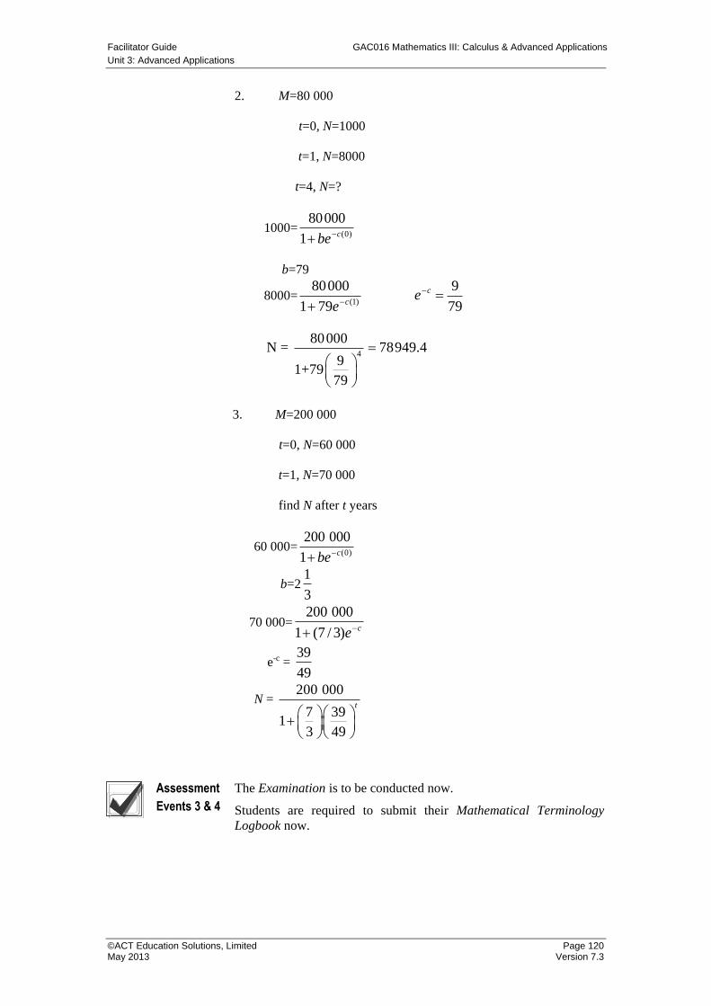
Facilitator Guide GAC016 Mathematics III: Calculus & Advanced Applications
Unit 3: Advanced Applications
©ACT Education Solutions, Limited Page 120 May 2013 Version 7.3
2. M=80 000
t=0, N=1000
t=1, N=8000
t=4, N=?
1000=(0)
80000
1 cbe
b=79
8000=(1)
80000 9
1 79 79
c
ce
e
4
80000N = 78949.4
91+79
79
3. M=200 000
t=0, N=60 000
t=1, N=70 000
find N after t years
60 000=(0)
200 000
1 cbe
b=21
3
70 000=200 000
1 (7 / 3) ce
e-c = 39
49
N = 200 000
7 391
3 49
t
Assessment
Events 3 & 4
The Examination is to be conducted now.
Students are required to submit their Mathematical Terminology
Logbook now.
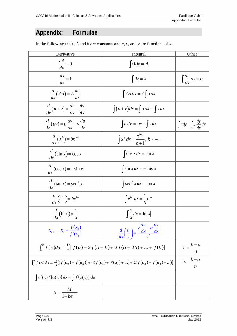
GAC016 Mathematics III: Calculus & Advanced Applications Facilitator Guide
Appendix: Formulae
Page 121 ©ACT Education Solutions, Limited Version 7.3 May 2013
Appendix: Formulae
In the following table, A and b are constants and u, v, and y are functions of x.
Derivative Integral Other
0dA
dx 0dx A
1dx
dx dx x
dudx u
dx
d du
Au Adx dx
Au dx A u dx
d du dv
u vdx dx dx
u v dx u dx v dx
d dv du
uv u vdx dx dx
u dv uv v dx dy
udy u dxdx
1b bdx bx
dx
1
, 11
bb x
x dx bb
sin cosd
x xdx
cos sinx dx x
(cos ) sind
x xdx
sin cosx dx x
2(tan ) secd
x xdx
2sec tanx dx x
bx bxde be
dx
1bx bxe dx eb
1
lnd
xdx x
1
lndx xx
1
( )
'( )
nn n
n
f xx x
f x
2
du dvv u
d u dx dx
dx v v
bfhafhafafh
dxxfb
a ...222
2
n
abh
b
an afafafafafaf
hdxxf ...2...4
3)( 42310
b ah
n
duxufdxxufxu )()()(
1 ct
MN
be