Level-Set and Phase-Field Methods: Application to Moving Interfaces and

Two-Phase Fluid Flows

Maged IsmailClaremont Graduate University

& Keck Graduate Institute

HMC Math 164, Scientific Computing, Spring 2007

Outline

• Background & Motivation• Level Set Method• Sharp-Interface Phase-Field Method• Conservative Level Set Method• Mathematical Formulation for Two-phase Flows• Conclusions & Future Work• Acknowledgments• References

Background & Motivation

• Tracking of moving interfaces- Wide range of scientific and engineering applications(e.g. two-phase fluid flows, melting and solidification, computer graphics, image segmentation- Typically two types of approaches to simulate moving interfaces:▪ Particle Methods (Lagrangian, explicit)

can’t handle topological changes, sharp corners…▪ Level Set Methods (Eulerian, implicit)

today’s topic

Level Set Method

• An implicit method for capturing the evolution of an interface.

• History: Devised by Sethian and Osher (J. Computational Physics,1988) as a simple and versatile method for computing and analyzing the motion of an interface in two or three dimensions.

• Based upon representing an interface as the zero level set of some higher dimensional function.

Level Set Method

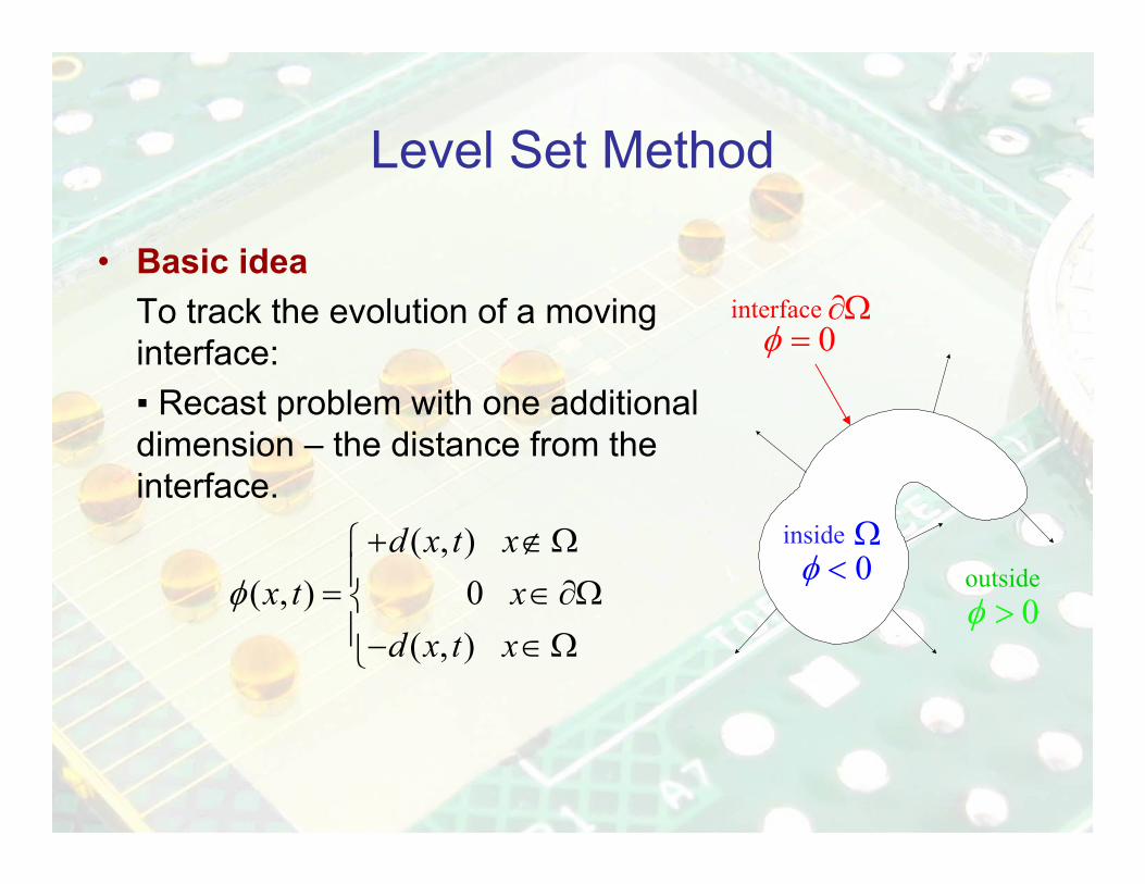
• Basic ideaTo track the evolution of a moving interface:▪ Recast problem with one additional dimension – the distance from the interface.

( , ) ( , ) 0

( , )

d x t xx t x

d x t xφ

+ ∉Ω⎧⎪= ∈∂Ω⎨⎪− ∈Ω⎩

0φ <0φ >

outside

inside

interface0φ =

Ω

∂Ω

Level Set Method

• The interface always lies at the zeroth level set of the function

• i.e., the interface is defined by the implicit equation

• To advance the interface:Given a velocity field, uThe evolution equation becomes:

• Interfacial geometric quantities can be easily calculated using

φ

( ), 0t x yφ =

φ| |,φ φ κ= ∇ ∇ =∇⋅n n

0tφ φ∂+ ⋅∇ =

∂u

Level Set Method

• Advantages:- capable of capturing topological changes- intrinsic geometric properties are easy to determine- relatively easy to implement- accurate high order computational schemes exist

• Difficulties:- computationally expensive- re-initialization is needed to maintain the signed distance function- not conservativeloss or gain of mass (area) due to numerical diffusion

Sharp-Interface Phase-Field Method

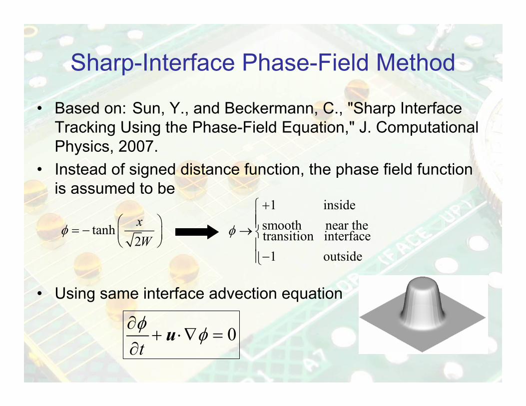
• Based on: Sun, Y., and Beckermann, C., "Sharp Interface Tracking Using the Phase-Field Equation," J. Computational Physics, 2007.

• Instead of signed distance function, the phase field function is assumed to be

• Using same interface advection equation

tanh2xW

φ ⎛ ⎞= − ⎜ ⎟⎝ ⎠

1 insidesmooth near thetransition interface

1 outside

φ

+⎧⎪⎪→ ⎨⎪−⎪⎩

0tφ φ∂+ ⋅∇ =

∂u

Sharp-Interface Phase-Field Method

• However, using

and

• The following evolution equation can be derived

• Descritized using finite difference method• Simple forward Euler for time discretization (explicit)• spatial discretization…

( )e a bκ= + −u u n( )21 φ φφκ φ

φ φ φ⎛ ⎞ ⎡ ⎤∇ ⋅∇ ∇∇

= ∇⋅ = ∇ ⋅ = ∇ −⎜ ⎟ ⎢ ⎥⎜ ⎟∇ ∇ ∇⎝ ⎠ ⎣ ⎦n

( )22

2

1ea b

t Wφ φφ φφ φ φ φ

φ

⎡ ⎤− ⎛ ⎞∂ ∇⎢ ⎥+ ∇ + ⋅∇ = ∇ + − ∇ ∇⋅⎜ ⎟⎜ ⎟∂ ∇⎢ ⎥⎝ ⎠⎣ ⎦

u

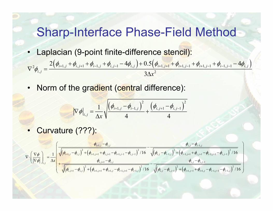
Sharp-Interface Phase-Field Method• Laplacian (9-point finite-difference stencil):

• Norm of the gradient (central difference):

• Curvature (???):

( ) ( )1, , 1 1, , 1 , 1, 1 1, 1 1, 1 1, 1 ,2, 2

2 4 0.5 43

i j i j i j i j i j i j i j i j i j i ji j x

φ φ φ φ φ φ φ φ φ φφ + + − − + + + − + − − −+ + + − + + + + −

∇ =Δ

( ) ( )2 2

1, 1, , 1 , 1

,

14 4

i j i j i j i j

i j xφ φ φ φ

φ + − + −− −∇ = +

Δ

( ) ( ) ( ) ( )

( ) ( )

1, , , 1,

2 2 2 2

1, , 1, 1 , 1 1, 1 , 1 , 1, 1, 1 , 1 1, 1 , 1

, 1 ,,2 2

, 1 , 1, 1 1, 1, 1 1,

/16 /161

/16

i j i j i j i j

i j i j i j i j i j i j i j i j i j i j i j i j

i j i ji j

i j i j i j i j i j i j

x

φ φ φ φ

φ φ φ φ φ φ φ φ φ φ φ φφφ φφ

φ φ φ φ φ φ

+ −

+ + + + + − − − − + + − − −

+

+ + + + − + −

− −−

− + + − − − + + − −⎛ ⎞∇∇⋅ =⎜ ⎟⎜ ⎟ −∇ Δ⎝ ⎠ +

− + + − − ( ) ( ), , 1

2 2

, , 1 1, 1 1, 1, 1 1, /16

i j i j

i j i j i j i j i j i j

φ φ

φ φ φ φ φ φ

−

− + − + − − −

⎛ ⎞⎜ ⎟⎜ ⎟⎜ ⎟

−⎜ ⎟−⎜ ⎟

⎜ ⎟− + + − −⎝ ⎠

ii-1 i+1 i+2

Need 4 points to discretize with third order accuracy φ∇

This often leads to oscillations at the interface

Fix: pick the best four points out of a larger set of grid points to avoid/minimize oscillations (“essentially-non-oscillatory”)

i-3 i-2 i+3 i+4

Set 1 Set 2 Set 3

Sharp-Interface Phase-Field Method• Hyperbolic term

(3rd order Essentially-Non-Oscillatory scheme)e φ⋅∇u

Sharp-Interface Phase-Field Method• Results

- Interface motion with a constant normal speedperiodic cosine curve propagating with normal speed of unity

( ) ( )0 1 , 1 cos 2 / 4 , 0 1s s sγ π= − + ≤ ≤⎡ ⎤⎣ ⎦

Swallowtail solution Weak solution (meaningful)

Analytical solutions Numerical solution

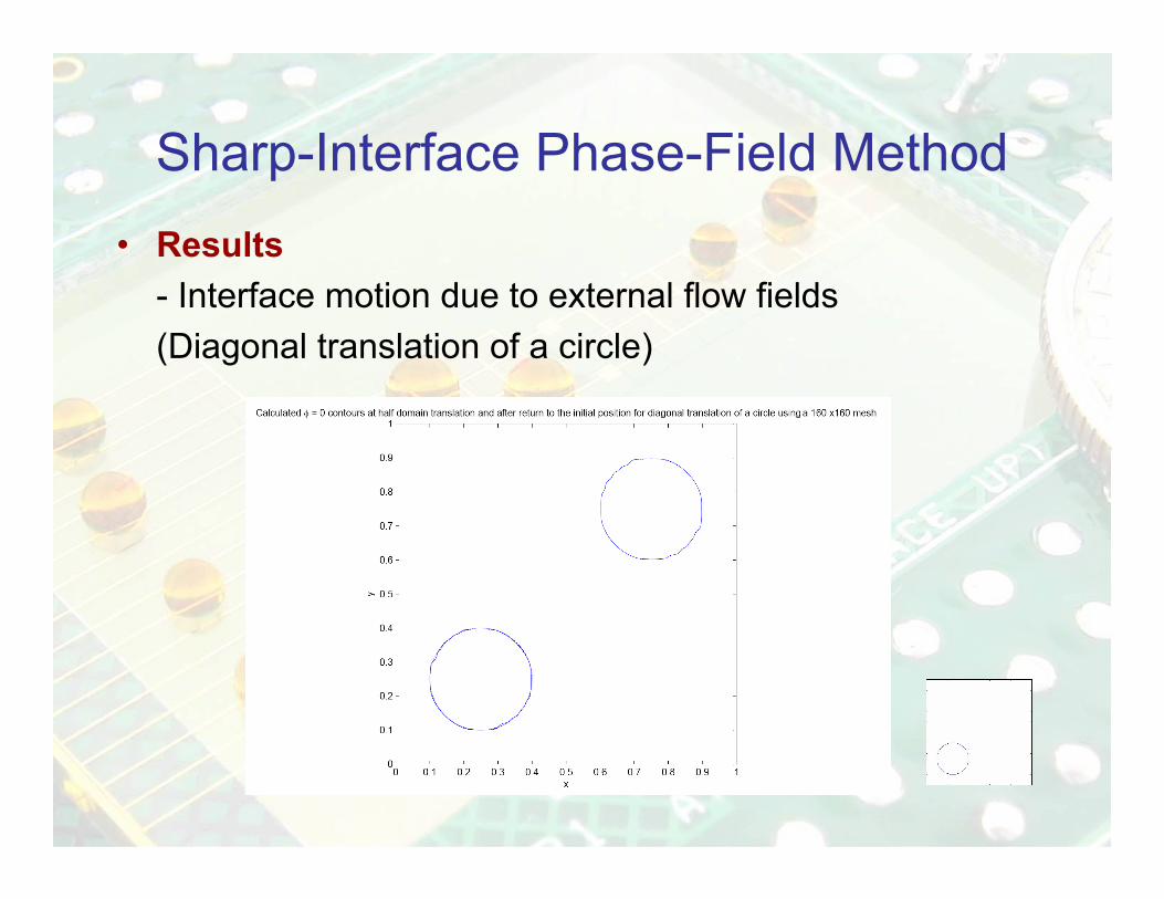
Sharp-Interface Phase-Field Method• Results

- Interface motion due to external flow fields(Diagonal translation of a circle)

Conservative Level Set Method• Based on :Olsson, E., Kreiss, G., A conservative level set method

for two phase flow, Journal of Computational Physics, 2005.• Level set function

smeared out Heaviside instead of signed distance function

where

• Interface represented by 0.5φ =

( )

0, ,1 1 sin , ,2 2 2

1, ,

sd

sd sdsm sd sd

sd

H

φ εφ πφφ φ ε φ εε π ε

φ ε

< −⎧⎪⎪ ⎛ ⎞= = + + − ≤ ≤⎨ ⎜ ⎟

⎝ ⎠⎪⎪ >⎩

φ

( ) ( ) ( )minsd dφΓ

Γ∈Γ= = −

xx x x x

Conservative Level Set Method

• Evolution equation of- Standard level set method

▪ loss or gain of mass (area) due to numerical diffusion▪ interface shape is not preserved

- Modified equation (non-conservative form): add▪ shape preserving artificial compression ▪ artificial diffusion to smear the profile (avoid discontinuities)

φ

0tφ φ∂+ ⋅∇ =

∂u

( )1tφ φφ γ ε φ φ φ

φ

⎡ ⎤⎛ ⎞∂ ∇+∇ ⋅ = ∇ ⋅ ∇ − −⎢ ⎥⎜ ⎟⎜ ⎟∂ ∇⎢ ⎥⎝ ⎠⎣ ⎦

u

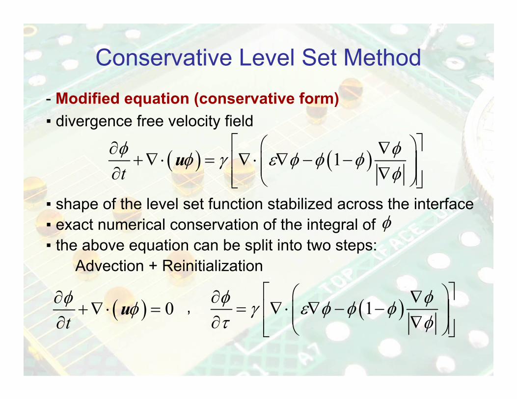
Conservative Level Set Method- Modified equation (conservative form)▪ divergence free velocity field

▪ shape of the level set function stabilized across the interface▪ exact numerical conservation of the integral of ▪ the above equation can be split into two steps:

Advection + Reinitialization

,

( ) ( )1tφ φφ γ ε φ φ φ

φ

⎡ ⎤⎛ ⎞∂ ∇+∇⋅ = ∇ ⋅ ∇ − −⎢ ⎥⎜ ⎟⎜ ⎟∂ ∇⎢ ⎥⎝ ⎠⎣ ⎦

u

φ

( ) 0tφ φ∂+∇ ⋅ =

∂u ( )1φ φγ ε φ φ φ

τ φ

⎡ ⎤⎛ ⎞∂ ∇= ∇⋅ ∇ − −⎢ ⎥⎜ ⎟⎜ ⎟∂ ∇⎢ ⎥⎝ ⎠⎣ ⎦

Mathematical Modeling of Two-phase Flows

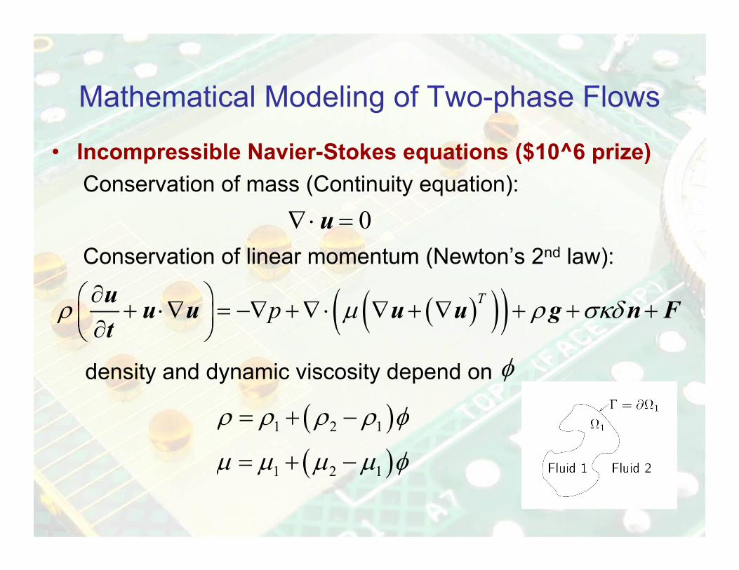
• Incompressible Navier-Stokes equations ($10^6 prize)Conservation of mass (Continuity equation):

Conservation of linear momentum (Newton’s 2nd law):

density and dynamic viscosity depend on

0∇⋅ =u

( )( )( )Tpρ μ ρ σκδ∂⎛ ⎞+ ⋅∇ = −∇ +∇⋅ ∇ + ∇ + + +⎜ ⎟∂⎝ ⎠u u u u u g n Ft

φ

( )1 2 1ρ ρ ρ ρ φ= + −

( )1 2 1μ μ μ μ φ= + −

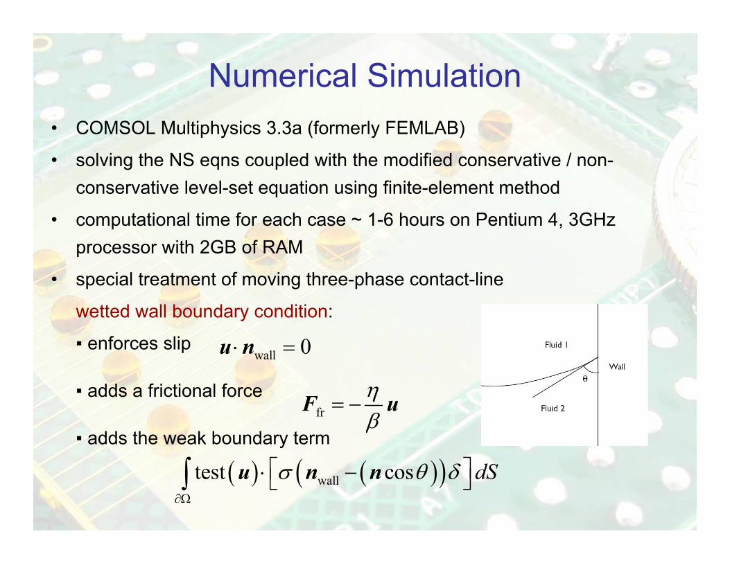
Numerical Simulation• COMSOL Multiphysics 3.3a (formerly FEMLAB)

• solving the NS eqns coupled with the modified conservative / non-conservative level-set equation using finite-element method

• computational time for each case ~ 1-6 hours on Pentium 4, 3GHz processor with 2GB of RAM

• special treatment of moving three-phase contact-line

wetted wall boundary condition:

▪ enforces slip

▪ adds a frictional force

▪ adds the weak boundary term

wall 0⋅ =u n

frηβ

= −F u

( ) ( )( )walltest cos dSσ θ δ∂Ω

⎡ ⎤⋅ −⎣ ⎦∫ u n n

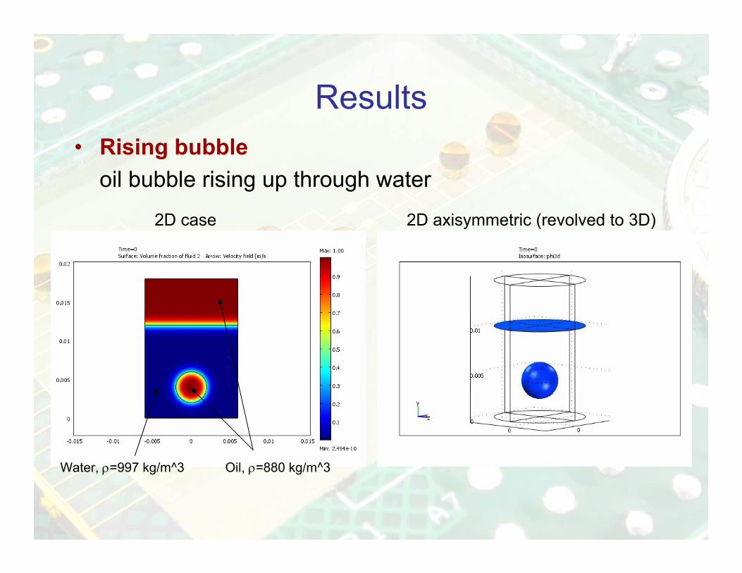
Results• Rising bubble

oil bubble rising up through water

2D case 2D axisymmetric (revolved to 3D)

Oil, ρ=880 kg/m^3Water, ρ=997 kg/m^3

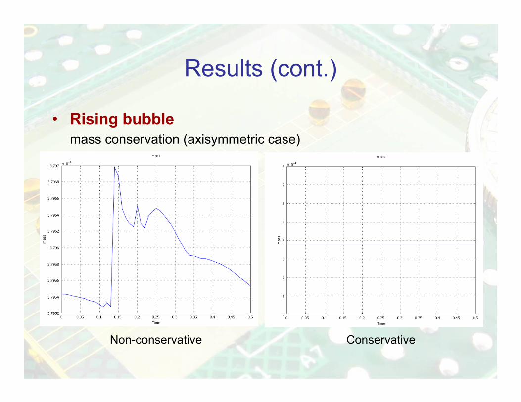
Results (cont.)

• Rising bubblemass conservation (axisymmetric case)

Non-conservative Conservative

Results (cont.)

• Falling droplet2D axisymmetric 2D axisymmetric (revolved to 3D)

Results (cont.)

• Droplet spreading (moving contact lines!)

zero gravity with gravity

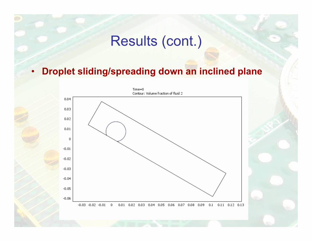
Results (cont.)

• Droplet sliding/spreading down an inclined plane

Conclusions

• Several variants of the standard level-set method exist.• Sharp-interface phase-field method implemented in

Matlab using FD discretization and used for tracking propagating interfaces.

• Conservative level-set method tested on several two-phase flow benchmark cases.

• Problems with moving contact-line also considered.

Future Work

• Validation with published experimental/analytical results• Implementing the sharp-interface phase-field method in

COMSOL Multiphysics• Application to droplet-microfluidics• Extension to three-dimensional cases (parallel-computing!)• Funding…proposals

Acknowledgements• Dr. Ali Nadim (KGI/CGU)• Dr. Darryl Yong (HMC)• Support from KGI/CGU

References

• Osher, S., Fedkiw, R. ,2003, Level Set Methods and Dynamic Implicit Surfaces, Springer.

• Olsson, E., Kreiss, G., 2005, A conservative level set method for two phase flow, Journal of Computational Physics, Vol. 210, pp. 225-246.

• Sun, Y., Beckermann, C., 2007, Sharp Interface Tracking Using the Phase-Field Equation, Journal of Computational Physics, Vol. 220, pp. 626-653.

Questions

Thank you!