777,7.Y',i

BMO TR-81-1

SAI DOCUMENT NO, SAI-79-506-VF LEVEL~SPERFORMANCE TECHNOLOGY PROGRAM

•p; (PTP-S II)

VOLUME III

INVISCID AERODYNAMIC PREDICTIONS FOR BALLISTIC REENTRYVEHICLES WITH ABLATED NOSETIPS

SCIENCE APPLICATIONS, INC,APPLIED MECHANICS OPERATIONWAYNE, PENNSYLVANIA(19087

SEPTEMBER, 1979

FINAL REPORT FOR PERIOD MARCH 1978 - SEPTEMBER 1979

S CONTRACT NO, F04701-77-C-0126

APPROVED FOR PUBLIC RELEASEj DISTRIBUTION UNLIMITED.ALL OF AFR 80-45 APPLIES.

AIR FORCE BALLISTIC MISSILE OFFICE DELECTEINORTON AFB, CALIFORNIA 92409 ElE_

NOO DEC 28 1981

D

81 12 23 117

This final report was submitted by Science Applications, Inc., 1200 ProspectStreet, La Jolla, California 92038, under Contract Number F04701-77-C-O126with the Ballistic Missile Office, AFSC, Norton AFB, California, MajorKevin E. Yelmgren, BMO/SYDT, was the Project Offiri.r in charge. This technicalreport has been reviewed and is approved for publication.

"J,

KEVIN E. YELMGREN, Majdr, USAFChief, Vehicle Technology BranchReentry Technology DivisionAdvanced Ballistic Reentry Systems

Ii

FOR THE COMMANDER

/ N HOLAS C. BELINIONTE, Lt Col, USAFDirector, Reentry Technology DivisionAdvanced BAllistic Reentry Systems

A!l

S-i

-Tr R-7 - ,

UNCLASSIFIEDSECURITY CL.ASSIFICATION OF THIS PAGEt (When Dnto Entered)

REPORT DOCUMENTATION PAGE RE~AD INSTRUCTIONS____________________________________ BEFORECOMPLETIXNGFORM

1. REPORT NUMBER 2.* GOVT ACCIESS N 0LO 3. RECIPICHY-AX-.ATALOG0 NUMBER

BMO TR-81-1 -5VJý

"Performance Technology Program (PTP-S II), Vol. Final Report: 3/78 to 9/79III, inviscid Aerodynamic Predictions for Bal -______________

listic Reentry Vehicles with Ablated Nosetips." SAI-79-506RGEPOTNVFE

7. AUTHOR(s) 11. CONTRACT 04 GRANT NUMUECRr)

Darryl W. Hall F04701 -77-C-Ol 26

9. PERFORMING ORGANIZATION NAME AND ADDRESS 10. PROGRAM ELEMENT. PROJECT. TASKCScience Appl ications, In:c. 169A OKUNTNM~fR994 Old Eagle School Rd., Ste. 1018 Task 3.2.1.2[ Wayne, Pennsylvania 19087

Ballistic Missile Office September ____1979

Norton AFB, California 92409 .NUBROPAE

14. MONITORIN`G AGENCY NAME & AOORESS(IU different fromi Contro~IIng Office) 1S. SECURITY CLASS. (of this report)

Uncl assifiedj I.. ECLSSFiCATION/ODOWNGRADING

1S. DISTRIBUTION STATEMENT (*I this Report)

Approved for public release; distribution unlimited.All of AFR 80-45 applies.

17. DISTRIBUTION STATEMENT (at the abstract entererd In Block 20. il dflfrmii Iro Repoirt)

I111 SUPPLEMENTARY NOTES

* 19. KZY WORDS (Continue on rev.erse aide It nsc~aamr and Identify by' bloc* nont be)

Flow FieldBlunt Body CodeReentry Veh'iclesAsymmetric NosetipsConformal Mapping

20. ABSTRACT (Continue atn revrse adid* it neoesasay and Identify' by bilock nwnber)

1,A three-dimensional inviscid time-dependent blunt body flow field code is'developed for calculation of hypersonic flow over ablated reentry vehiclenosetips. The code is formulated in a coordinate system that is based on

* a sequence of conformal mappings and is capable of being aligned witharbitrary nosetip shapes. This procedure includes a finite differencescheme that permits the automatic calculation of embedded shocks in anapproximate manner. -

Do FOM 1473 UNCLASS I FIEDSECURITY CLASSIFICATION OF THIS PAGE (Whein Daet Entered)

UNCLASSIFIED ? P@f. la

89CNROS fCLA uIRIATINOl MI Aed)Do3S~

20- AUS1TACT (Cnsfawad)

BLANK PAGE

Ik

UN CLASSIFIED ___________

3, SgatatelNl C.L.ASSIVICATION OF THIS PA49grwha, Data "1;.ed)

, --"' 717,"

_"-'ý -w" . M•- ____.......___

TABLE OF CONTENTS

Page

ABSTRACT (DD1473) . . ... . i

TABLE OF CONTENTS . . • 1

LIST OF FIGURES .... 3

NOMENCLATURE . . ... 6

SECTION 1 INTRODUCTION . . ... 9

SECTION 2 PROBLEM DEFINITION . ... 15

2.1 STATEMENT OF THE PROBLEM . . 15

2.2 OUTLINE OF APPROACH . . •18

SECTION 3 COORDINATE SYSTEM AND GOVERNING EQUATIONS • 22

3.1 INVISCID EQUATIONS OF MOTION 22

3.2 THREE-DIMENSIONAL CONFORMAL TRANSFORMATION 26

3.3 TRANSFORMED EQUATIONS OF MOTION . . . 40

3.4 COMPUTATIONAL TRANSFORMATION • , . 44

3.5 CHARACTERISTIC RELATIONS . . .. 52

3.6 TREATMENT OF THE SINGULAR CENTERLINE , *,. 58

SECTION 4 CALCULATION OF EMBEDDED SHOCKS . ' 67

4.1 CONSERVATION LAW APPROACH TO SHOCK-CAPTURING . . 67

4.2 X-DIFFERENCING APPROACH TO SHOCK-CAPTURING . . 75

4.3 COMPARISON OF AXISYMMETRIC SHOCK-CAPTURINGPROCEDURES • . . . . . . '80

4.4 X-DIFFERENCING SCHEME IN THREE DIMENSIONS • ,. 88

SECTION 5 NUME'1V PROCEDURES . . . . . . (91

5.1 TIME-ASYMPTOTIC SOLUTION & INITIALIZATION' . .91

5.2 NON-CONSERVATION FIELD POINT TREATMENT • • 95

5.3 BODY POINT TREATMENT . . . . . . 97

1.

I1

TABLE OF CONTENTS (Cont'd.)

5.4 BOW SHOCK POINT TREATMENT . . .. 100

5.5 CENTERLINE POINT TREATMENT . . . . 105

5.6 CONSERVATION FIELD POINT TREATMENT . . . 109

5.7 X-DIFFERENCING FIELD PO•INT TREATMENT . . . 112

SECTION 6 VALIDATION OF SOLUTION . . . . . . 114

6.1 LIMITATIONS OF TECHNIQUE . . . . . 114

6.2 CONVERGENCE PROPERTIES . . . 116

H 6.3 VALIDATION OF NOSETIP SOLUTION . . . . 123

6.4 PREDICTION OF TOTAL VEHICLE INVISCIDAERODYNAMICS . . . . . . . 136

SECTION 7 CONCLUSIONS . . . . . . . . 156

SECTION 8 REFERENCES • • . . . . • . 160

SECTION 9 APPENDIX: COEFFICIENT3 FOR THE SHOCK ACCELERATIONEQUATION . .. 163

Accession For

1rTIC TAR

Justification

Di.stribuation~/

Availability Codes O T ICfvail and/or ELECTE

2.

-zU 7_ ___ __

LIST OF FIGURES

Figure Page

1.1 Typical Nose Shape Progression 1.. 10

1.2 Schlieren Photograph of Ablated Nosetip withEmbedded Shock . . .. 13

2.1 Rea-Mm Map of Flow Regimes with Typical ReentryVehicle Trajectory Superimposed . . .. 16

3.1 Hinge Point Definition . . .. . . 29

3.2 Hinge Point Images (Sphere) . . . . . 31II3.3 Plane Hinge Point Images and Body Contour (Sphere) •33 ,

3.4 Body Contour in Transformed Plane for 50O/I0OBiconic Nose . . . . . .. 36

3.5 Body Contour in Transformvd Plane for Very

Mildly Indented Body . . . . . 37

3.6 Body Contour in Transformed Plane for PANT Triconic 38

3.7 Body Contour in Transformed Plane for IndentedNose Shape . . . . . .. 39

3.G Computational Mesh for Spherical Nose . • 49

3.9 Computational Mesh for PANT Triconic . . . 50"Li

3.10 Computational Mesh for Indented Nose Shape . . 51

3.11 Cartesian Coordinate System at the Centerline 6 .60

3.12 Unit Vectors at Centerline . . . 64

4.1 Steady inclined Shock . . . . 68

4.2 Unsteady Normal Shock . . . 70

4.3 Characteristic Slopes in x-t Plane . . 774.4 Shock Shape Predictions for VMIB at M. = 7.2 81

4.5 Surface Pressure Predictions for VMIB at M. 7.2 . 82

4.6 Effect of Damping on Shock Shape Predictionswith Conservation Scheme . . . . . . 84

3.

"a W A

LIST OF FIGURES (Cont'd.)

Figure Page

S4.7 Shock Shape Predictions for MI8 at M. 9 . . . 865.1 Numerical Domain of Dependence for Regular

MacCormack Scheme , . , 110

5.2 Typical Aligninent of Embedded Shock in Y-Z5.3Coordinate Mesh . . .. 111

S5.3 Numerical Domain of Dependence for MacCormackScheme Inverted in Z-direction , , 112

6.1 Typical p0 History (Converged) . . . . 119

6.2 Typical p0 History (Not Converged) . . . . 120

6.3 Typical (CT/G)rms History (Converged) . . , 121

6.4 Typical (CT/G)rms History (Not Converged) , . . 122

6.5 Shock Shape Predictions for a Sp;iere inEquilibrium Real Gas . . .. 125

6.6 Predictions of Surface Pressure Distribution fora Sphere in Equilibrium Real Gas . . . . 126

LI 6.7 CM3DT(NC) Prediction of Surface Pressure Distributionfor the PANT Triconic (with Cone) at M - 5, a = 00 . 128

6.8 CM3DT(NC) Prediction of Surface Pressure Distributionfor the PANT Triconic (without Cone) at M. = 5, a = 00. 129

6.9 CM3DT(X) Prediction of Surface Pressure Distribution

for the PANT Triconic (with Cone) at M= = 5, a a 00 130

6.10 CM3DT Shock Shape Predictions for the PANT Triconicat M. = 5, a = 00 .. 3

6.11 Surface Pressure Predictions for the PANT SimpleBiconic at M. = 5. . . .= . 133

6.12 Bow Shock Shape Predictions for the Blunt-1Shape at M. = 13.4, t = 30 . . .. 135

6.13 Surface Pressure Predictions for the PANTTricon,;c at M = 5, a = 100 . . . 137

6.14 Normal Force and Pitching Moment Coefficients vs.Angle of Attack for 90 Sphere-Cone of 15%Bluntness at Mr, 20, a = 00 . . . 139

II 4.

LIST OF FIGURES (Cont'd.)

Figure page6.15 Pitch Center of Pressure vs. Bluntness Ratio

for 9c Sphere-Cone at M 20, 50, a - 00 • 141

6.16 Normal Force and Pitching Moment Coefficients vs.Angle of Attack for 9' Sphere-Cone of 15% Bluntnessat M® a 20,8w5O . . . . . . 142

5.17 Normal Force Coefficient vs. Angle of Attack forBlunt-1 Configuration at M - 13.4, 20 KFT Altitude . 143

6.18 Pitching Moment Coefficient vs. Angle of Attack forBlunt-! Configuration at M 13.4, 20 KFT Altitude 144

6,19 N8 Confiquration 146

6.20 Normal Force ,oefficient vs. Angle of Attack forN8 Configuration at M= - 8 . . . . 148

6.21 Pitching Moment Coefficient vs. Angle of Attackfor N8 Configuration at M 8 . . . 149

6.22 Normal Forc:e Coefficient vs. Angle of Attackfor VMIB Configuration at MW 11.6 . . 151

6.23 Pitching Moment Coefficient vs. Angle of Attackfor VMIB Configuration at M,, = 11.6 , 152

6.24 Normal Force Coefficient vs. Angle of Attackfor MIB Configuration at M,, - 11.6 . , 153

6.25 Pitching Moment Coefficient vs. Angle of Attackfor MIB Configuration at M,, = 11.6 . . 154

6.26 Pitch Center of Pressure vs. Angle of Attack forVMI3 and MIB ConIgurations at M • 11.6 . 155

I 5

5. I

[I

NOMENCLATURE

a isentropic speed of sound

ak stretching coefficient in * k plane

AB vehicle base area, nRB

b(&,O) body surface in (En.0) space

c(E,8,T) bow shock surface in (•,ne) space

CN normal force coefficient, FN/qAB

C pitching moment coefficient, Mz/q1 ,ABL

Ccos(-W)

Sd shock layer thickness

e total energy per unit volume

FN normal force

9 /constant

gj azj+IOzjl -constant

G IgIh static enthalpy, or altitude

thhij,k hinge point i in jt- transformed plane in * = *k plane

H total enthalpy

i -

ISM unit vectors in (¢,n,8) space

unit vectors in (x,y,¢) space

L reference length

LA vehicle length, measured from virtual apex

M Mach number

Mz pitching moment

n unit normal vector

p pressure

6.

'• - -~..... ... ....... ..."' " - - • .. . .

PO stagnatior pressure

P logar'ithm of pressure

q dynamic pressure, I/2pV 2

R gas constant

RB vehicle base radius

RN vehicle nose radius

Re Reynolds number

i entropy

s non-dimensional entropy, g/R

Ssin (w)

t time coordinate in (x,y,O) frame

T time coordinate in (Xi',Z) frame

UVW velocity components in (x,y,o) space

u,v,w velocity components in (•,nB) space

u normal velocity component

velocity vector

V magnitude of velocity vector

v tangential velocity component

W shock velocity

x,y,¢ cylindrical coordinates in physical space

Xlx, x Cartesian coordinates at centerline

X,Y,Z computational coordinates

x moment reference pointcg

x cp pitch center of pressure location

zk x+iy in = k plane

zj,k imaqe of zk in jh- transformed plane

damping coefficiencs for conservation calculations

7.

angle of attack

SCI trim angle of attack

8 sideslip angle

y isentropic exponent

6 boundary layer thickness

6j,k exponent for Jh conformal transformation in 0 - *, planea0 bow shock stand-off distance

V ýk E+in in ,=k plane

eb body slope

A characteristic slope

'1. viscosity

coordinates in transformed space

SL(6) downstream boundary of computational region in transformedspace

p density

a shock slope

T time coordinate in (En,e) frame

ýl + i42 B(log g)/Bý0 = constant

w arg (g)

"( )b quantity at body surface

( )s quantity at bow shock

( ). freestream quantity

8.

SECTION 1

INTRODUCTION

Current research efforts in ballistic reentry vehicle aero-

dynamics are prim~rily concerned with the;improvement of vehicle targeting

accuracy. Accurate evaluation of possible targeting errors requires a

detailed understanding of all mechanisms that may deflect the vehicle

away from its nominal ballistic trajectory. Of the dispersion errors

that can be attributed directly to the reentry vehicle, the low altitude

roll-trim effect is one of the prime contributors to miss distance.

Roll-trim dispersion results when normal forces, such as

created by a trim angle of attack condition, are not integrated out by

the spin of the vehicle. The characterization of such dispersion re-

quires a coupling of the vehicle's dynamics with its aerodynamic charac-

teristics along the entire entry trajectory. This effort is aimed at ex-

tending current aerodynamic prediction capabilities relative to the low

altitude roll-trim dispersion problem.

The current generation of ballistic reentry vehicles are

typically slender blunted cones or biconic configurations, with the nose-

tips generally being fabricated from woven carbonaceous materials. During

reentry the severity of the aerothermodynamic environment causes ablation

of the nosetip material, leading to both axial recession of the nosetip

and to alterations in the basic shape of the nose.

At higher altitudes (100 KFT • h k 50 KFT) the flow in the

nosetip boundary layer remains laminar, resulting primarily in blunting

of the nosetip. Below approximately 50 KFT, however, as the nosetip

boundary layer is passing through transition to a fully turbulent

9.

state, the increased heating levels lead to a sharpening of the nosetip

shape, as illustrated in Figure 1.1.

Because of circumferential variations in the onset and pro-

gression of nosetip transition, asymmetric nose geometries can result.

The mechanisms governing this transition process, such as surface rough-

ness variations,are generally evaluated statistically, as by Dirling.

I!

!I

LAMINAR

r

TRANSITIONAL TURBULENT

Figure 1.1. Typical Nose Shape Progression

10.

f.. . I

The development of an asynmmetric nosetip shape on an otherwise

axisynrietric body will lead to the development of a trim angle of attack

and corresponding side forces which ten'] to deflect the vehicle from its

ballistic trajectory. To minimize these trim effects, reentry vehicles

are punprio tother renteingthe tmopher; tus he itegate

resultant of a body-fixed lift force over one revolutior' of the body will

be nearly zero. However, rapid variations in nose shape and angle of

attack (and hence lift force) and roll rate can result in a non-zero

resultant force, leading to trajectory deflection due to roll-trim dis-

persion.

Because of the inherent uncertainties in nose shape change

predictions, the roll-trim effect is usually evaluated statistically,

as by Pettus, Larmour, and Palmer 2 . Given a nose shape, however, the

evaluation of aerodynamic characteristics, a necessary part of any roll-

trim evaluation, is a deterministic problem.

Aside from expensive and time-consuming wind tunnel tests, the

most accurate and reliable method for the prediction of aerodynamic

characteristics is the numerical integration of the invsicid equations

of fluid motion. Fortunately, at the flight conditions of interest (and

in most hypersonic wind tunnels simulating reentry conditions at low

altitudes) the Reynolds number is sufficiently large that the shock

layer is almost entirely inviscid, except for the thin boundary layer

adjacent to the vehicle surface. Additionally, the flow is in the weakj

interaction regime, as defined in Hayes and Probstein 3 , where viscous

shear and induced pressure effects significantly affect only the axial

force experienced by the vehicle. Other vehicle forces and moments

(normal and side forces, pitching and yawing moments) can then be

accurately determined solely through consideration of the inviscid

pressure distribution.

In the past decade many tiumerical procedures have been developed

for the calculation of inviscid aerodynamic characteristics for ballistic

reentry vehicles. These techniques have proven to be valuable adjuncts

to the design process and have, to some extent, lessened the neA.d of

performing extensive wind tunnel tests to validate proposed configurations.

The three-dimensional numerical proceiures currently in use consist of

two parts: a transonic flow field procedure to treat the subsonic region

surrounding tne stagnation point, and an afterbody procedure to treat the

the supersonic flow on the vehicle frustum.

The inviscid afterbody flow field problem is now well in hand

for the simple axisymmetric frusta found on ballistic reentry vehicles.

(In addition, ballistic vehicles at low altitudes generally do not

develop large angles of attack which would lead to flow separation on

the leeside of the afterbody, invalidating the inviscid assumption.) The

existing inviscid transonic nosetip flow field capability is restricted,

however, to convex shapes, where strong embedded shock waves, such as

shown in the Schlieren photograph in Figure 1.2, do not occur. Further-

more, other restrictions arise even for convex shapes, when the coordinate

system used in the calculation is not closely aligned with the surface of

the nosetip. (These shortcomings of the current techniques were identi-

fied by Hall, Kyriss, Truncellito, and Martellucci .

12.

H .. . . .

.1A

.I

i

Figure 1.2. Schlieren Photograph of Ablated Nosetip with Embedded Shock

13.

I ,.fL.

The goal of the current research effort is to eliminate the

above two restrictions on inviscid transon'ic flow field techniques. By

extending the range of nosetip shapes that can be analyzed numerically

to include slender and indented shapes-such as have been observed in

flight, the capability for accurate evaluation of roll-trim dispersion

will be greatly expanded. In addition this nrw capability will allow

more accurate nose shape reconstruction efforts (in which a nose shape

is sought that produces aerodynamic characteristics that agree with

those derived from the vehicle motion observed in flight), as described

by Hall and Nowlans Furthermore, this transonic flow field technique

will be applicable to maneuvering as well as ballistic reentry vehicles,

since autopilot design for maneuvering vehicles must account for the

aerodynamic characteristics that result from ablated nosetip geometries.

The approach taken to eliminate these deficiencies of the

current nosetip flow field procedures is outlined in Section 2.2.

.4Section 3.0 details the conformal mapping transformation used to produce

a coordinate system closely aligned with the body surface, and Section

4.0 describes the procedures used for the calculation of embedded shocks.

In Section 5.0, details are provided on the numerical procedures used in

this new transonic flow field technique, which is validated by compari-

sons to data in Section 6.0.

41

14.

r1 _

SECTION 2

PROBLEM DEFINITION

2.1 STATEMENT OF THE PROBLEMrThe problem being examined in this research effort involves

the numerical prediction of the inviscid aerodynamic characteristics

of ballistic reentry vehicles with asymmetric, ablated nosetips. In

particular, emphasis is placed on the development of a numeric.1 tech-

nique to determine the inviscid flow field about a three-dimensional,

asymmetric nosetip ir a uniform hypersonic or supersonic freestream flow.

The determination of the nosetip flow field is a necessary first step

for the prediction of total vehicle aerodynamics.

The assumption is made in this analysis that inviscid flow

theory is adequate to accurately predict the aerodynamic characteristics

of reentry vehicles at altitudes where asyfmietric nose shapes can result

from ablation (h s 50 KFT). (Accurate calculation of drag forces will

also require consideration of surface shear and induced pressure effects,

however.) Implicit in the assumption of inviscid flow are the require-

ments that the thin boundary layer assumption be valid and that no regions

of separated flow exist on the vehicle.

Moretti and Salas , in their analysis of viscous rarefied

fhiows, have presented a breakdown of the various flow regimes that might

be expected as a function of freestream Mach and Reynolds numbers (with Ithe Reynolds number based on nosetip radius for a spherical nose), as

depicted in Figure 2.1. Also indicated in this figure is an M, - Re,

history for a typical modern ballistic reentry vehicle as a function ofi . I

altitude. Defining the thin boundary layer regime as the region where

15.

CD 1

'IUI--

CDwIJ w wV 0-

LAJ LaJ W .

LC J LA -J V

CD u~

+ 0 0:

o 0>-

cooW b~wnNH-V

o16.

the boundary layer thickness (6) is less than 1% of the shock layer

thickness (d), this figure clearly indicates the validity of the in-

viscid assumption for the probler' being considered here.

The hypersunic flow over a blunt nosetip is char~cterized by a

detached bow shock wave separating the shock layer from the undisturbed

freestream flow. In the vicinity of the stagnation point, where the

bow shock is nearly normal to the freestream velocity vector, the flow

in the shock layer is locally subsonic; thus, the steady flow problem in

this region has an elliptic character. As the bow shock curves back

1 I around the body and becomes more oblique to the freestream velocity

vector, and as the shock layer flow expands around the nose, the flow

becomes locally supersonic, and the steady flow problem becomes hyper-

bolic. Other complications can arise in this basic inviscid flow field

structure if the body surface has indented regions producing embedded

shock waves. Depending on the shock strength, the flow behind such an

embedded shock could be either subsonic or supersonic.

Because of this variety of flow conditions that can be en-

countered in the blunt body problem, it is convenient to seek the steady

solution as the asymptotic limit of the time-dependent problem, since

the unsteady flow equations are hyperbolic in time, regardless of the

local Mach number. Furthermore, since the location of the bow shock

wave is unknown a priori and must be determined as part of the solution

procedure, this time-asymptotic approach has the additional benefit of

allowing the calculation of the time history of the shock shape starting

from an assumed initial shock position.

The numerical procedure to be used in the solution of this

time-dependent problem is an explicit, second-order accurate finite-

17.

'I J• •

difference piiceoure. Similar schemes have been developed previously,

and are cuirently in wide use; however, these procedures are limited in

their ability to treat slender ablated nosetip shapes, and in their

ability to treat embedded shocks. This research effort is devoted to

the development of a procedure that eliminates the deficiencies observed

in other transonic time-dependent codes. In particular, this requires

development of a generalized Coordinate system that is capable of being

closely aligned with the three-dimensional body surface for abritrary

body geometries, as well as the development of a procedure for the cal-

culation of three-dimensional embedded shocks on indented nosetip shapes.

Coupling this nosetip tvdisonic procedure to an existing

supersonic afterbody code will thus allow accurate theoretical assess-

• ment of the effect of ablated nosetip geometries on the performance of

the total vehicle for many nose shapes that could not previously be

ana'yzed.

S2.2 OUTLINE OF APPROACH

The fuidamental approach selected in this research effort for

the solution of the blunt body problemT. for ablated asymmuetric nosetips

is the time-dependent relaxtion approach. This technique has been widely

used in previous work and has several advantages directly related to

difficulties associated with the blunt body problem. In particular, thetime-dependent approach allows the use of a convenient forward-marching

(in time) numerical algorithm, avoiding many of the difficulties other-

wise encountered in the steady flow problem.

The numerical scheme selected for this analysis is in many ways

similar to that used in other procedures. For example, the treatment of

II18.

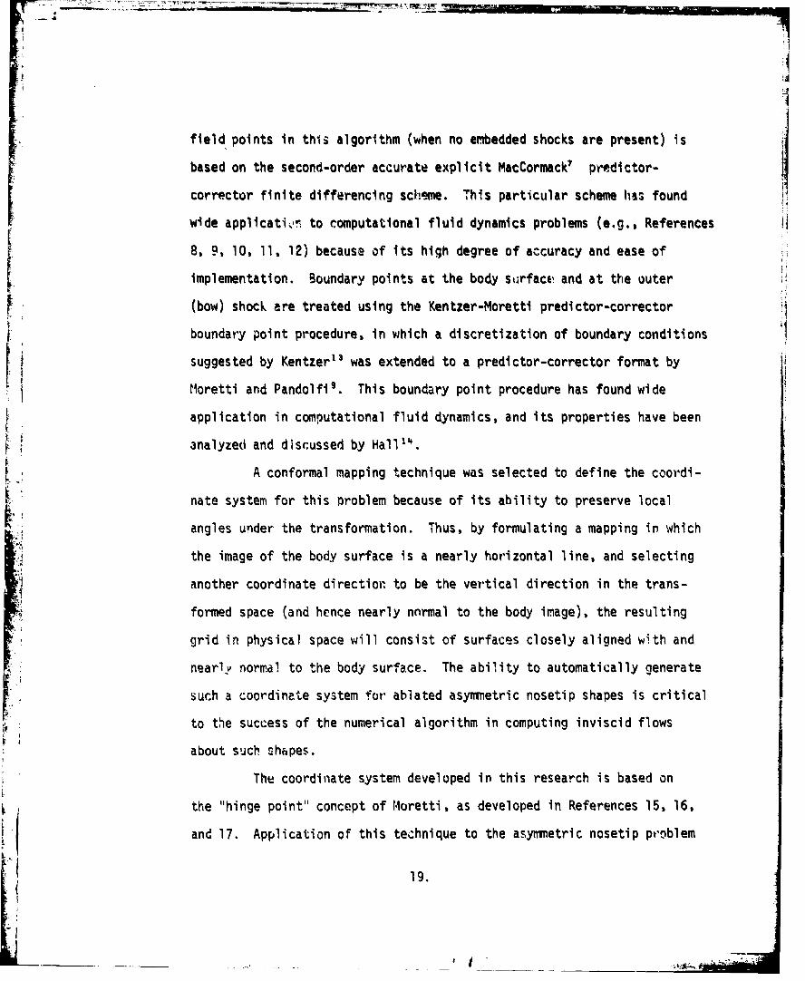
field points in this algorithm (when no embedded shocks are present) is

based on the second-order accurate explicit MacCormack? predictor-

corrector finite differencing scho.me. This particular scheme has found

wide applicatir,• to computational fluid dynamics problems (e.g., References

8, 9, 10, 11, 12) because of its high degree of accuracy and ease of

implementation. Boundary points at the body stirface and at the outer

(bow) shock are treated using the Kentzer-Moretti predictor-corrector

boundary point procedure, in which a discretization of boundary conditions

suggested by Kentzer1 3 was extended to a predictor-corrector format by

Moretti and Pandolfi9. This boundary point procedure has found wide

application in computational fluid dynamics, and its properties have been

analyzed and discussed by Hall'.

A conformal mapping technique was selected to define the coordi-

nate system for this problem because of its ability to preserve local

angles under the transformation. Thus, by formulating a mapping in which

the image of the body surface is a nearly horizontal line, and selecting

another coordinate direction to be the vertical direction in the trans-

formed space (and hence nearly nnrmal to the body image), the resulting

grid in physical space will consist of surfaces closely aligned with and

nearly normal to the body surface. The ability to automatically generate

such a coordinate system for ablated asymmetric nosetip shapes is critical

to the success of the numerical algorithm in computing inviscid flows

about such shapes.

The coordinate system developed in this research is based on

the "hinge point" concept of M~oretti, as developed in References 15, 16,

and 17. Application of this technique to the asymmetric nosetip pr'oblem

19.

has required the extension of this technique to three dimensions; this

development is described in Section 3.2.

To treat the embedded shock problem in this research effort,

the shock-capturing approach has been selected, in which the structure of

the embedded shock is approximated, but for which no special logic is

required to explicitly treat the shock. Two shock-capturing approaches

are examined: the conservation formulation, discussed in Section 4.1, !

and 'the X-differencing approach, discussed in Section 4.2. Axisymmetric

versions of both of these techniques have been developed, and a comparison

of the results of these two approaches is made in Section 4.3. Based on

these comparisons, it is concluded that the X-differencing approach is

the superior method, and, accordingly, is extended to three-dimensions in

Section 4.4.

Axisytrmetric, inviscid, time-dependent proceiures with a shock-

capturing approach to the treatment of embedded shocks have, of course,

been developed previously, notably by Kutler, Chakravarthy, and Lombard18

(using the conservation form) and by Moretti" (using the X-differencing

approach). The successful application of the X-shock-capturing technique

to the three-dimensional time-dependent embedded shock problem is, however,

new.

The final portion of this effort is devoted to the validation

of the resulting numerical technique for the calculation of inviscid nose-

tip flow fields. For simple nosetip shapes (e.g., spheres) this new

technique is compared to proven flow field codes, such as that developed

by Kyriss and Harris 8 . For other shapes, representative of nosetip shapes

that result from the ablation process, comparisons are made with wind

20.

tunnel measurements of surface pressure and bow shock shape. Un-

fortunately, most of the existing wind tunnel data providing these details Ion nosetip flows are available only for axisymmetric shapes, as in

Reeves, Todisco, Lin, and Pallone20 and Jackson and Baker".

A large body of wind tunnel data does exist for the total aero-

dynamics of reentry vehicles with asymmetric nosetips. Coupling the new

nosetip flow field procedure to an existing afterbody code, comparisons I

are made between predicted and measured vehicle forces and moments, thus

providing an indirect means of verifying the accuracy of the nosetip

calculation. These comparisons are presented in Section 6.4.

21.

,Am=

' SECTION 3

•i COORDINATE SYSTEM AND GOVERNING EQUATION•S

This section provides details on the coordinate transformation

developed in this effort that is capable of mapping the surface of

ablated, asymmetric nosetip geometries ,•ntk) a nearly horizontal surface,

thus producing a coordinate grid cl0oszly aligned with the body geometry.

This mapping is then used to generate the three-dimensional inviscid

time-dependent equations of fluid motion written in terms of the new

coordinates. A final computational transformation is described that

maps the transformed shock layer onto a regular, equally spaced grid.

The equations derived in this section are written in non-

i conservation form; i.e., the dependent variables are the primary flow

variables. This form of the governing equations is the form used for

flow calculations when embedded shocks are not present, and as the basis

of the X-differencing shock-capturing scheme described in Section 4.2.

The conservation form of the governing equations is discussed in Section

4.1.

3.1 INVISCID EQUArIONS OF MOTION

The three-dimensional time-dependent inviscid equations of

asP + UP + VP S + WP/Y + y(U + VI + W/y + V/y) 0 (3.1)

Ut + UUx + VU y + WU¢/ + pPx/P= 0 (3.2)

Vt + UVx + VVy + WV /y -W2/y + p~yp /= 0 (3.3)

22.

W + UWx + V14 + WW /y + VW/y + pP /py =0 (3.4)

St + UsX + Vsy + Ws¢/y= 0 (3.5)

where

AA

with I, J, and K being the unit vectors in the x, y, and * directions,

respectively. (In this cylindrical system, x is the axial, y the radial,

and * the circumferential coordinate.) In this formulation the dependent

thermodynamic variables are P and s, where

P = £n p (3.6)

and s is some suitable analog of the entropy. The choice of P as a

dependent variable is motivated by computational considerations, since

the logarithm of pressure throughout the shock layer will not vary by

several orders of magnitude as the pressure might; thus, one can expect

more accurate finite difference representations of derivatives of P than

could be expected for p.

For closure of this system of partial differential equations,

a thermodynamic equation of state of the form

p = p(p,s) (3.7)

is required. For an equilibrium real gas calculation, the relation em-h~4

bodied in Equation (3.7) may be provided either through tabulations of

the thermodynamic properties or through an appropriate curve fit of the

thermodynamic data. In the case of a thermally and calorically perfect

(ideal) gas, this thermodynamic relation may be expressed implicitly as

23.

s = (2n p -yknpV(y-l) (3.8)

where the thermodynamic variable s is defined in terms of the entropy

S as

s = (s- (3.9)

with y the isentropic exponent and R the gas constant. Inversion of

Equation (3.8) yields

1-Ysi/Y _YSp p e .(3.10)

Finally, to complete the definition of the mathematical problem,

initial and boundary conditions must be specified. Since the steady-state

solution is sought as the asymptotic limit of the transient problem, the

specification of an initial flow field is required. Details on the de-

finition of this assumed initial flow field are presented in Section 5.1.

Boundary conditions for this problem must be specified at

the boundaries of the region being computed: at the bow shock wave

y= Ys (x,c), on the body surface y - Yb(X,), and on some downstream

boundary, running between the body and the shock. The location of the

downstream boundary is arbitrary, subject only to the restriction that

the flow across this boundary be supersonic. As long as this boundary

is entirely supersonic, no condition need be imposed there, since the

range of influence of this boundary will then not extend back into the

region being computed.

At the bow shock, whose position is unknown a priori and

must be determined as part of the solution procedure, the appropriate

boundary conditions are given by the familiar Rankine-Hugoniot conditions.

24.

i -. -- "••• •_• '• - _ _ _ _ _ _ _ _ _ _ _ __=_ __...._ _

By incorporating differential forms of these relations for conservation

of mass, momentum, and energy across the shock into a characteristic

compatibility relation, an equation for the shock acceleration is obtained,

which may be integrated to yield shock velocity and position. This

numerical scheme is described in more detail in Section 5.4.

At the body the appropriate boundary condition to be imposed

is the inviscid kinematic boundary condition, which requires that there

be no velocity component normal to the body surface. This condition is

applied in conjunction with a characteristic compatibility condition to

develop a numerical procedure for body points as described in Section 5.3.

Also of interest in the treatment of boundary conditions for

this problem is the value of entropy that applies along the streamline

that wets the body surface. It is frequently assumed that the surface

entropy for inviscid flows is exactly the normal shock value of entropy,

but this can be proven only for axisymmetric flows. Numerical results

of Swigart 22 and the experimental results of Xerikos and Anderson "

indicate that this assumption may not be true and that the normal shock

streamline does not wet the body surface. However, in his survey paper,

Rusanov2 4 argues that the results of Swigart's calculations using ank inverse method are inconclusive because of the inherent assumptions and

computational errors. Additionally, Rusanov points out that his own

computational results using a finite difference procedure produced

variations between the computed surface entropy and the normal shock

entropy of less than 0.1%, which is within the error level of his calcu-

lation. From the examination of his studies and the results of others,

Rusanov concludes that there is no firm evidence of the surface entropy's

25.

not having the normal shock value, although there is likewise no

proof that these values coincide.

From a practical standpoint, the question of the value of the

surface entropy is not critical, since even the variations in surface

entropy claimed by Swigart and Xerlkos and Anderson produce only small

perturbations on the other flow variables (e.g., density, velocity).

Accordingly, the body surface is assigned the known normal shock value

of entropy in this problem.

Circumferentially, the boundary condition to be imposed in

this problem is that of periodicity; i.e., the solution at 0 = 0 must

coincide with the solution at € = 27. For the case of a pitch plane of

symmetry (geometric symmetry and no sideslip), the calculation need be

performed only from € = 0 to 7 = w, and the circumfev'ential boundary

conditions simply require symmetry about the pitch plane.

3.2 THREE-DIMENSIONAL CONFORMAL TRANSFORMATION

A major portion of this research is devoted to the development

of a generalized, three-dimensional coordinate transformation that is

capable of producing a coordinate surface closely aligned with the body

surface. As outlined earlier, the method that has resulted is based on

an idea of Moretti's 17 for axisymmetric time-dependent calculations.

The general coordinate transformation used takes the functional

form 4S= ~(~,)(3.11)

n= n(x,y,4') (3.12)

(3.13)

.t (3.14)

26.

t•

which implies that the transformation of the spatial coordinates is

independent of time. Furthermore, * = constant planes are transformed

directly to e = constant planes, thus retaining a somewhat "cylindrical"

quality to the transformation.

Prior to reentry, ballistic vehicles are initially axisym-

metric, and it may thus be expected that ablated asymmetric nosetip

shapes that develop during reentry will retain some "axisymr!n'ric"

character. In other words, since the * constant planes wil. be normal

to the vehicle surface prior to reentry, it is reasonable to expect that

the simple transformation 8= will lead to e = constant planes that are

nearly normal to the surface of the ablated nosetip, even though the

ablated shape may not be truly axisymmetric.

Within each @ = constant plane, then, the transformation re-

duces to the form (

V {x,y) (.S

= r,(x,y) . (3.16)

Since it is desirable to have a coordinate grid closely aligned with

the body geometry (and hence with the streamlines of the flow), a

transformation is sought that closely aligns the • direction with the

body surface 'within a * = constant plane). In order to have the

n-ýdirection normal to the &-direction at all points land hence nearly

normal to the body surface), a conformal transformation is sought, since

under a conformal transformation, the orthogonal (x,y) grid maps onto

an orthogonal (&,n) grid.

"27.! 27.

Ii ! I!'ii

Conformal transformations from the zI x + ly space to I]

the { - + in space can then be developed independently in each *-plane.

These transformations rely on the concept of "hinge points" as developed

by Moretti 1'•16,17 to ensure that the t-direction is closely aligned with

the body surface.

The concept behind this "hinge point" approach is to define

a sequence of points in the zI1 space that lie close to the body surface

and define an approximate equivalent body shape. A sequence of con-

formal transformations is then applied to map each of these hinge points

in turn onto the horizontal axis; if the hinge points in the zI space .

accurately simulate the body contour, the resulting transformed contour

will then be nearly horizontal (i.e., will be closely aligned with a A

coordinate surface).

"For the mapping function developed in this research, which

has been adopted by Moretti 17 for axisymmetric calculations, hinge points

are defined as illustrated in Figure 3.1. Let h denote the ii,j,k

hinge point in the jth transformed space (j = 1 is (x,y) space) in the (J

= *k plane. It is required that hlk be located on the nosetip

centerline outside of the body and that h2 lk be located on the center...

line inside the body. The remaining hinge points hilk, i 3,4,...,JC

"•' are selected so as to model the body contour. Note from Figure 3.1 that

this specification of points produces JA = JC - 2 "corners" which must

be &Iiminated by the mapping sequence to have all hinge point images on

the horizontal axis (in the transformed space).

28.

-at

I.

z

0 CI-

z

LU

LU-

29.

To eliminate each corner in succession, the mappings, which

have been developed as part of this effort, of the form

zj+lk - 1 J,k - hj+lIk, k (3.17)

are applied sequentially for j = 1, 2,...,JA. The form of this transforma-

tion is related to the Schwarz-Christoffel transformation and indeed may

be regarded as a"point-wise" Schwarz-Christoffel transformation. By

proper selection of the exponents 6j,k' defined from I

ITI

-j,k -tan- Im hj+2,j,k - hj+lljk (3.18) 1

Reh+ 2 ,j,k " hj+l,j,k]

these mappings have the required property of maintaining all hinge

points hi,j,k, i t j on the real axis, while mapping hj+l,j~ k onto the

real axis. I

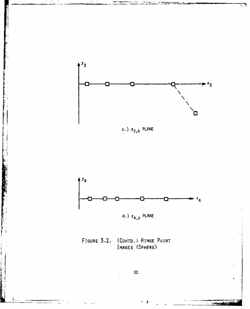
The application of this mapping is illustrated in Figure 3.2,

showing how each of the JA corners is eliminated successively, resulting

in all hiJBk (with JB JA + 1 = JC - 1) lying on the real axis in

the ZJB,k space. It is important to note that straight line segments

between hinge points in the zlk space are not maintained as straight

segments under this sequence of transformations. Since each of these

intermediate transformations is conformal, the sequence of mappings will

itself be a ccnformal transformation.

30.

MIRK

ra.) zk PLANE

l~4

FtY

V2

b. z PLNE

2,kFIGRE .2.HINE PINTIMAES SPHRE

31

y3

I,

kY33

V C-) Z3,k PLANE

4Y

d.) Z4,k PLANE

FIGURE 3.2. (CONTD.) HINGE POINT

IMAGES (SPHERE)

32.

___c.)__3,kPANE

Two further transformetlons are required to complete the

sperificatlon of a suitable coordinate grid. First, it is beneficial

to have the transformed body contour (which is now aligneA closely with

the horizontal a.xis in the ZJBk space) nearly perpendicular to theimage of the centerline, which runs between hlJBk and h2,JB,k (and is

still a s- *aight line). Accordingly, a simple square root conformal

transformation may be applied in the formn

ZJCk = ZJB,k - h2,JB,k)"/ (3.19)

leading to the hinge point alignment shown in Figure 3.3. Also shown in

this figure is the resulting body surface contour for the simple case of

a sphere, using the hinge points shown in Figure 3.2.

- I

n = b(C)

FIGURE 3,3. C PLANE HINGE POIN'T IMAGES AND

BODY CONTOUR (SPHERE)

33.

Because the sequence of transformations defined-above is

carried out independently in each 0 a Ok plane, there is no necessary

correspondence between hinge point image locations in these planes,

except that h2,JCk a 0 and Re (hl,JC,k) - 0 for all Ok" In order to

minimize the discrepancies that must arise between these mappings along

the centerline (which is common to all *k planes), a final stretching is

applied in each plane to ensure that the hinge point images h1,JCk

coincide in the k= + ini space. This goal is attained by setting

= ak ZJC~k (3.20)

with the real coefficients ak defined by

ak h /hJC,I/hlJC,k (3.21)

This simple scaling is itself a conformal transformation and thus

preserves the orthogonal nature of the (ý,n) grid. (Note that the (E,n,e)

space is not, however, necessarily orthogonal.)

It is important to note that while the final images of

h,l,k and h have the same values in the {k space that only those

two points along the centerline have direct correspondence in the zI ,k

space. Because of different scale factors that arise from the independent

conformal transformations in each Ok plane, points with the same C

value do not necessarily correspond to the same point in the Zlk planes.

34.

Although the conformal mappings in each *k plane are defined

independently, the global transformation may be considered continuous

by requiring that che governing parameters of the transformation be

continuous functions of * and that each *k plane have the same number

of hinge points (JC). In particular, this requires that the functions

a(O), h2,j,(¢), hj+l,j(¢), and 6j(o) be continuous.

The success of this mapping sequence is illustrated in

Figures 3.4 - 3.7. Shown in these figures are longitudinal nosetip

profiles that are characteristics of low altitude, turbulent ablation of

initially spherical carbonaceous nosetips. In each case, the hinge

points used in the transformation are indicated in the zI plane, as well

as the body contours that result in the { plane. These figures indi-.a -e

the flexibility inherent in this conformal mapping procedure, allowing

any arbitrary nosetip contour to be mapped onto a nearly horizontal line.

4 Figures 3.5 and 3.6 represent postulated axisyrrmetric nosetip shapes that

have been tested in wind tunnels: the Very Mildly Indented Body (VMIB),

as reported by Reeves, Todisco, Lin, and Pallone 20 (Figure 3.5) and the

PANT Triconic, as reported by Jackson and Baker" (Figure 3.6). Figure

3.7 represents a profile of the indented nosetip shown in the Schlieren

photograph in Figure 1.2, which was recovered from a flight test.

The process of mapping the body contour onto a nearly hori-

zontal line is relatively insensitive to the selection of hinge points,

as long as the hinge points approximate the body shape in some reasonable

fashion. Thus, the selection of hinge points is easily automated by

spacing them at a fixed distance along inward body normals (in the (xy)

plane) from body points equally spaced in wetted length.

35.

-- - .- - " -- -- - -: -~.;:LI : I

y

1.0 ZPLANE

0.5

IIl 3 R 0 0.5

so*0.5-

R 0-.5

0- 0 0.5 1.0

0.4 C PLANE

00.4 0.8 1.2}.-

FIGURE 3.4. BODY CONTOUR IN TRANSFORMEDPLANE FOR 50°/10° BICONIC NOSE

36.

I . . • • •- • - ..

I y

zPLANE

K ~2.0-42.13 - 3

H1.0

0 no0"I I i -

0 1.0 2.0 3.0

0.4 - C PLANE

c•,0 0.4 0.8 1.2 1.6 2.0

FIGURE 3.5. BODY CONTOUR IN TRANSFORMED PLANEFOR VERY MILDLY INDENTED BODY(20 )

4 37.

C-v] -7

y

z PLANE

2.0 .

00 2.0 4.0

0.4 SO. 4C PLANE

0 0.4 0.8 1.2 1.6 2.0

FIGURE 3.6. BODY CONTCJR IN TRANSFORMED

PLANE FOR PANT TRICONIC( 2 1 ),.1

38.

IOWA

y

zI PLANE 13

0.4

[I

0.2

0 o 10 3x

0 0.2 0.4

0.2

SPLANE

LI I

0 0.2 0.4 0.6 0.8 1.0

FIGURE 3.7. BODY CONTOUR IN TRANSFORMED

PLANE FOR INDENTED NOSE SHAPE

39.

--- - -- - --

:I

3.3 TRANSFORMED EQUATIONS OF MOTION

Using the mapping from (x,y,4,t) space to (&,no,e,T) space

described in the preceding section, the governing inviscid equations

(Equations (3.1)-(3.5))may be transformed to ({,net) coordinates by

application of the chain rule. Recalling the functional dependence of

the transformation defined in Equations (3.1l)-(3.14), the appropriate 4

i4A chain rules take the forms(I

at (3.22)

"-) a a (3.23)

a" y a- + "y an (3.24)

a + T, 1-* +. (3.25)

it is ccu•venient to define, using the notation of Moretti17,

g a Cei = G(C- iS) (3.26)g:az1

and

= a(log g) = + i(3.27)

with

G = Igl (3.28)

w - arg(g) (3.29)

40.

- J_

- cos (-w) (3.30)

- sin (-W) (3.31)

From the definition of the conformal transformation, it follows that

k a g /2ZJC (3.32)Jul k .ik

with

J= 6 jk (zj+l,k " l)/(Zj,k " hj+l,j,k)

and

JA ia = 1 9 {91g2...9J (610k )/(zj k-hj.-l ,j ,k)) (3.34) +takZJC,k g j=1 '(3)

With these definftions, the partial derivatives required

by the chain rules are found to be

x= GC (3.35)

y= GS (3.36)

.nx = -GS (3.37)

ny= GC (3.38)

41.

:114,!

Note that these forms verify that the mapping c = • (z1 )

in any € = constant plane is conformal, since the Cauchy-Riemann

conditions

x -y (3.39)

{y = -nx (3.40)

are satisfied.

Circumferential variations of the mappings are accounted

for with the equations (derived from a Taylor series expansion)

4) = + inr - [t 2 -tl-g(z2-zI)]/(€ 2 -€I) (3.41)

g, = [g2 -g1-g2 0 (z 2 -z 1)]/(z2-zl) (3.42)

where

C c2 =(x2Y2

l= g(xl'yl 4I

g2 = g(x 2,y 2 '42 )

with (xl,Yl,,l) and (x2 ,Y2,, 2) representing computational grid points in

surrounding @ planes; i.e., OI = -" A, 2 = + AO.

42.

It is convenient to write the governing equations in terms

of velocity components in the (g,n,e) space. Defining

V = uT + v3 + wk (3.43)

with Ti, 3, and k being unit vectors in the E,n, and 0 directions,

respectively, the new velocity components may be written in terms of

the cylindrical velocity components (U,V,W) as

u = u,+ VS (3.44)

v = -Uý + Vz (3.45)

w = W (3.46)

In terms of these velocity components, the governing equations14in non-conservation form may be transformed, using the chain rules de-

fined above, to

DP-

D•P+ y[G(u, + vn + v¢2 - u$ 1 ,

+ (f w + no w + w0 + uS + vC)/y] =0 (3.47)

TDu+ + +n01 + +e

- Sw2 /y + GpP{/p = 0 (3.48)

Dv +Tt~Dv uG(v4l + u0 2 ) _ uw(Eo2 + n€€ + We)yDT-

- Cw2/Y+ GpPn/p = 0 (3.49)

43.

iI

'ii

,I

+ w(uS + vC)/y + + P + Pe)/py = 0 (3.50)

Ds_0 (3.51)

where

_- -+ (Gu + w%/y) + (v + wn,/y)

+ W/Y a

The term we can be evaluated from

1 = Im{ge/g} (3.52)

with g. expressed as

g g " g (3.53)

3,A COMPUTATIONAL TRANSFORMATION

Prior to obtaining numerical solutions of the transformed

governing equations, it is convenient to perform an additional coordinate

transformation to map (•,ner) space onto a rectangular computational

space (X,YZ,T), in which an equally spaced mesh can easily be established

to facilitato numerical approximations of derivatives. In this computa-..--In:aI s:.-:,• the coordinate Z is selacted so as to be 0 on the body

Isurface and 1 o the outer boundary (bow shock wave) of the region of i

interest. S4.,,ilarly, Y is defined as being 0 on the centerline and 1 at

the downstr:.. : boundary of the region to be computed. X is directlyproportional to the circumferential coordinate e.

44.

I•

This computational transformation is described mathematically

as

X 8/e27r (3,54)

Y =/Le)(3.55)

Z = nb{e][(,,)b{e](3.56)

T T (3.57 N/

where the body surface is described as

Tj ({e (3.58)

I and the bow shock position as

n = (•,e•) .(3.59)

The downstream boundary is defined by

S={ (e ) .( 3 .6 0 )A

LIL

Because the position of the bow shock varies with time

during the solution of the time-dependent problem, the computational

grid also varies with time, but always maintains equally spaced points

between the body and bow shock (in Z).

To transform the governing equations into the computational

coordinates, the following chain rules are applied:

asT

X = y(3.5)

T-Y a +Z (3.62)

45.

Z nbi8)((,~)b~e](.6 S.. . . . . .. ,

azn (3.63)

a x 1- +Y + Z (3.64)

where

Xe 1/27r

iy• = llAL(e)L

Y 6 M "YY Le

Zn l/[c(f,e,T)-b(ý,e)J

z -ZnI(1-Z)br + Zc{]

Z6 -Zn[(l-Z)b 0 + Zc ]

" ~Z = -ZZnCT

with the body and shock slopes in the transformed srace being determined

from

= (Cybx - S)/(Sybx + C) (3.65)

be Gybo/(SYbx + b- + n@ (3.66)

c (CYsx - S)/(Sysx + C) (3.67)

ce = Gyso/(Sysx + ) - c + T¢ . (3.68)

46.

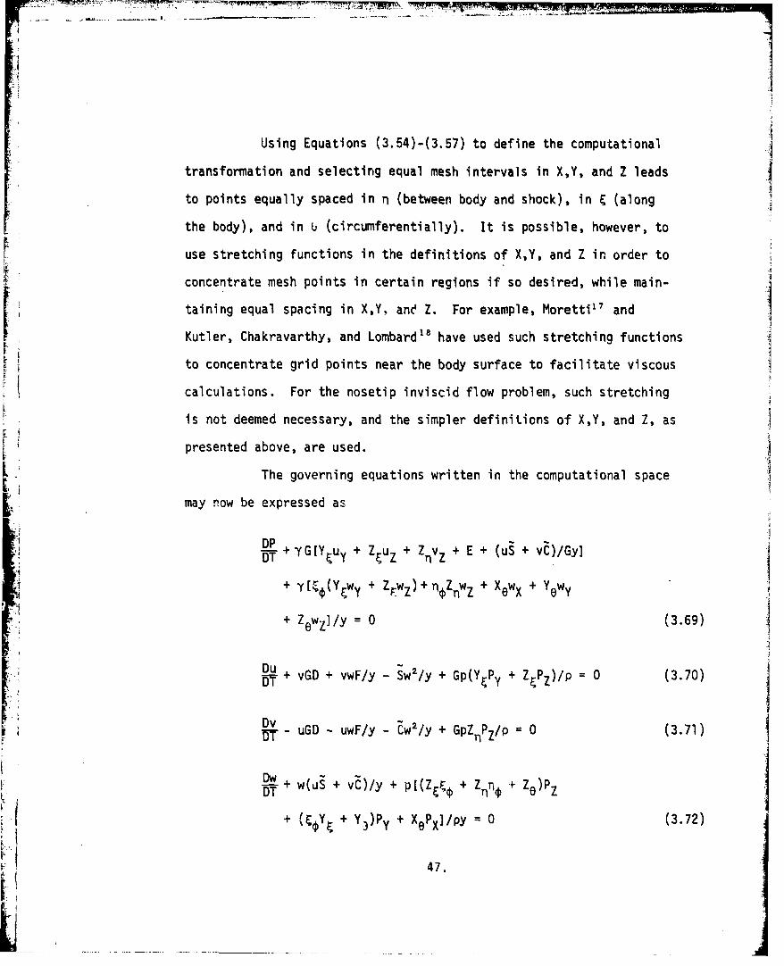
Using Equations (3.54)-(3.57) to define the computational

transformation and selecting equal mesh intervals in X,Y, and Z leads

to points equally spaced in n (between body and shock), in ý (along

the body), and in 6 (circumferentially). It is possible, however, to

use stretching functions in the definitions of X,Y, and Z in order to

concentrate mesh points in certain regions if so desired, while main-

taining equal spacing in X,Y, anc Z. For example, Moretti"' and

Kutler, Chakravarthy, and Lombard" 8 have used such stretching functions 4

to concentrate grid points near the body surface to facilitate viscous

calculations. For the nosetip inviscid flow problem, such stretching

is not deemed necessary, and the simpler definiticns of X,Y, and Z, as

presented above, are used.

The governing equations written in the computational space

may now be expressed as

DP + YG[Y uy + Z uz + Z vz + E + (uS + vC)/Gyl

+ Y[(Ywy + Zwz) + nZrn'Z + XewX + Y wy

+ Zewz]/y : 0 (3.69)

Du S2y+G(D7-+ vGD + vwF/y - SwY/y + Gp(Y•Py + Z•Pz)/p = 0 (3.70)

4D--- uGD - uwF/y - Cw2/y + GpZ Pz/P = 0 (3.71)

DW+DT w(US + vC)/y + pI(Zr + Z + Z)Pz

i + Y + Y)Py + X=Px1/pY 0 (3.72)

47.

-1

Ds 0 (3.:73)DTi

with

DT +' . + A - + B B - + C -

A =Z + (Gu + w& /y)Z• + (Gv + wn¢/y)Zn + wZ /y

B = (Gu + w& /y)Y + wy /Y

C = wX /y

D = v1+u¢

I= +-

F + n + € + We

Typical grids (in physical space, € = constan.t) that result

from this computational transformation are shown in Figures 3.8-3.10.

(In these figures, the bow shock shape used in defining the computational

region is an assumed initial bow shock shape.) For clarity in these

figures, a coarser grid is shown than would actually be used in the

calculation of a flow field about such bodies.

It is important to note in these figures that the { constant

lines are indeed nearly normal to the body surface, as is expected when

the image of the body contour is nearly horizontal (n = constant) and

the mapping is conformal. The generation of such grids was the goal

in the development of the mapping function presented here, and will

greatly expand the range of nosetip shapes that can be successfully computed.

48.

0.8 y

0.6

0.4

0. 2

oI , I

0-0.4 -0.2 0

FIGURE 3.8. COMPUTATIONAL MESH FOR SPHERICAL NOSE

49.

hi.

-

-

i I1

y

3.0i

A

3.1--

2.0-i

I m

I

0 l. 2.0 3.0

• 4 FIGURE 3.9. COMPUTATIONAL MESH FOR PANT TRICONIC(21)

II 50.

Ay

1.0-

K 0.5-

0 0.5

IFIGURE 3.10. COMPUTATIONAL MESH FOR INDENTED

NOSE SHAPE

51.

3.5 CHARACTERISTIC RELATIONS

The numerical procedures to be used at body and bow shock

points (which will be discussed in Sections 5.3 and 5.4) are based

on the characteristic compatibility relations resulting from the

governing system of partial differential equations, Equations (3.69)-

F (3.73). Accordingly, the appropriate forms of these compatibility

relations at the body and bow shock are derived in this section.K In the theory of partial differential equations a charac-

teristic surface is a surface across which the derivatives of the

dependent variables may be indeterminant in the direction normal to the

surface. The characteristic compatibility condition is a linear combi-

nation of the governing equations valid along this characteristic surface.t For use in this analysis, characteristics in the (Z,T)

reference plane are of interest; X and Y derivatives appearing in the

governing equations will be treated as forcing functions. Reduction of

the four-dimensional (X,Y,Z,T) problem to two dimensions results in a

characteristic curve, rather than a characteristic surface.

The governing equations may be rewritten as

PT + APz + yG(Z uz + Znvz)

+ y(E• z + nZ + Ze)wZ/y = R1 (3.74)

uT + Auz + GpZ Pz/p = R2 (3.75)

VT + Avz + GpZnPz/p = R3 (3.76)

WT + Awz + p(t.ZE + noZn + Zo)Pz/py = R4 (3.77)

52.

IiI

where

R= -[BPy + CPX + YG(Y uy + E + V/Gy)

+ Y(E Y wy + X Ywx Y wy)/y]

R2 -[Buy + Cu X + vGD + vwF/y - Sw 2 /y

+ GpY Py/PI

R3 = -[Bvy + CvX - uGD - uwF/y - Cw2/y]

R4 = -[Bwy + CwX + w(uS + vC)/y

c+ p{nieYr + YO)Py + xePxu/pyi

r!(The equation for entropy convection, Equation (3.73), is not

considered here, since it is known that the characteristic resulting

from its inclusion is simply a streamline. 'While a streamline is a

valid characteristic, it is not of immediate interest for this application.)

Defining the characteristic curve as

f(T,Z) 0 (378)

the normal to this curve is

= Vf =(ffZ) (3.79)

and the characteristic slope may then be defined as

_fT =(3.80)fz

53.

H • .. ' '•• • " -- '-- • -•• -r .. .. •..... - • ".. . ..' ........ .. ." r ... ., , • ' l

j I1

The characteristic compatibility condition is written as a linear

combination of the governing equations, where £I' £2. L3 and £4 are

the as yet undetermined multipliers for Equations (3.74)-(3.77),

respectively. Combining terms, the compatibility condition can then

be written as

SIP T + [t1A + Gp(Z 2Z( + z3Z )/p + £4 P(ycZ{ + nrZn + Ze)/PylP•

+ £2UT + (z 1yGZ{ + z2A)uz + k3VT + (£IYGZn +2 v ZyZn+k ,A]v

+ I4WT + [zlYZiZI + nvZn + Ze)ly + X4A]wz iiRi (3.81)

The terms involving derivatives of P may be regarded as a

directional derivative in the direction ýl, where

[£1 [ {A + GP(ZZ + Zn)/p + x z

+ Z + Z )/py]. (3.82)

Similarly, derivatives of u,v, and w may also be viewed as directional

derivatives in the directions w2 ,ý 3, and

2 = [12 ,£ 1YGZE + Z2A] (3.83)

W3 = [(3 IYGZn + £3A] (3.84)

q4 =[£•4{k1 y(.¢Z + n tZn+Ze)/y + k4A}] (3.85)

54.

For Equation (3.81) to be valid along the characteristic,

these directional derivatives must not have any component along the

direction of the normal to the characteristic curve (in which direction

the derivatives may be indeterminant). These conditions may be expressed

= = 1 " q3 q4 0 . (3.86)

Noting that -X this system of equations may be written in

matrix form as

A-X GpZ /p GpZ /p P(E z +n Zn+Zo)/PY zl

yGZ( A-x 0 0

yGZI 0 A-, 0 Z3

YU(y z+n Zn+Ze)/y 0 0 A-X 4 (3.87)

For a solution to this system of homogeneous equations to

exist, it is necessary that the determinant of the coefficient matrix

vanish. Furthermore, any one of the four unknowns may be scaled arbi-

trarily. Expansion of the determinant results in the following algebraic

equation:

(A-)2[(A- aG 2Z 2 2G2Z 2

-a 2 (•@Z+ + + Zn)2/y 2 ]= 0 (3.88)

55. '

-H,

L 1 .. _

where the isentropic speed of sound is defined from

a-- (yp/p)1 / 2 . (3.89)

The four roots to this equation are

X= A (redundant root) (3.90)

andSl + n Zn + ZB)]/ (3.91)

X= Aa [G2(Z•2 + Zn 2) +T 1+ (3

The redundant root X = A simply shows that streamlines are characteristic

directions, but, as stated earlier, this relation is not of immediate

interest. Thus, the characteristic slopes being sought are those defined

by Equation (3.91).

To evaluate the unknown multipliers Ri' it is convenient to

select Z.1 = 1; it then follows that

Z2 = yGZ /(X-A) (3.92)

k 3 =yGZn/(x -A) (3.93)

4 & = .Z + n Z + Z ')/(X-A)y (3.94)

The compatibility condition will then take the final form

PT + XPz + z2 (UT + XUz) + (VT + XVz)

+ z4(WT + XwZ) = 2.iRi (3.95)i=l

56.

To derive forms of this relation valid at the body, it is jfirst necessary to write the kinematic boundary condition in (Q,n,e)

space. Denoting the body normal as

b= -Gb•1 + G3 + (n -•b•-bb)/y k (3.96)

the boundary condition becomes

-Gub + Gv + 0 b (3.97) 4

The coefficient A, defined as

A Z + (Gu + WEo/y)Z + (Gv + wy)Zn + wZo/y

can be shown to vanish at the body since, with Z = 0,

Z=0 Z

Ze = -Znb

Ze = "Z b°

and thus

A Zn [-Gub + Gv + w(n-obE-be)/y] 0

from Equation (3.97). Choosing X < 0 at the body and simplifying the

expression for X yields

Xb =aZn [G 1+b + (-n¢,FobI-b /Y (3.98)

b In

V 57.

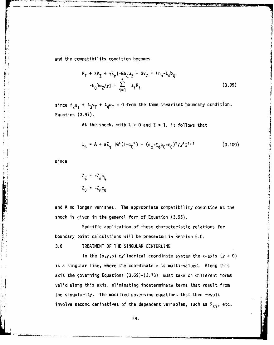
and the compatibility condition becomes

+ xPz + YZ[-Gb uz + GVz + -'4

-be)wz/y] = R (3.99)i =1

since k2UT + z + z 4WT 0 from the time invariant boundary ccndition,

Equation (3.97).

At the shock, with X > 0 and Z 1, it follows that

Xs A + aZn [G2 (l+c, 2 ) + (n,-_cc-c,)2/y2i" 2 (3.100)

since

Z= -Z c '1

-1

and A no longer vanishes. The appropriate compatibility condition at the

shock is given in the general form of Equation (3.95). iSpecific application of these characteristic relations for

boundary point calculations will be presented in Section 5.0.

3.6 TREATMENT OF THE SINGULAR CENTERLINE

In the (x,y,¢) cylindrical coordinate system the x-axis (y = 0)

is a singular line, where the coordinate € is multi-valued. Along this

axis the governing Equations (3.69)-(3.73) must take on different forms

valid along this axis, eliminating indeterminate terms that result from

the singularity. The modified governing equations that then result

involve second derivatives of the dependent variables, such as PXY' etc.

58.

In order to avoid these second derivatives, other approaches

to the centerline problem may be used. For example, the governing equa-

tions can be reformulated in a local Cartesian coordinate system, which[does not exhibit singular behavior. Approximation of derivatives in

the Cartesian space would, however, require extensive interpolation on

the data at the computational grid points which are not aligned with thef. Cartesian coordinates.In this analysis, a set of governing equations based on the

Cartesian approach at the centerline is developed which minimizes the

need for interpolation, while simultaneously avoiding the approximation

of second derivatives. (For the three-dimensional conformal mapping

approach developed in this research effort, the approximation of second

derivatives at the centerline is made particularly difficult by the fact

that the transformations used in each * plane are independent and thus

are not continuous across the centerline.)

To develop the form of the governing equations desired at A

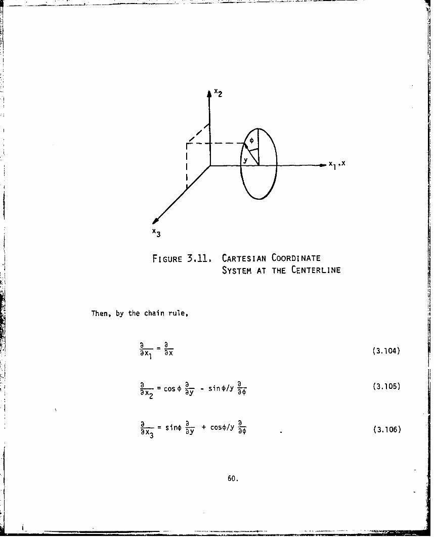
the '.anterline, consider a Cartesian reference frame (x1,x2 ,x ), oriented j

with the (x,y.ý) cylindrical system as shown in Figure 3.11, and defined

by

=i X (3.101)

= y Cos4 (3.102)

x3 =y sincý (3.103),

x2

IIx2

x3

FIGURE 3.11. CARTESIAN COORDINATE

SYSTEM AT THE CENTERLINE

Then, by the chain rule,

-xI 3 x (3.104)

(3.105)x2 os siny

___ - + isne/y

a ix3 + cosD/y y (3.106)

60.

Derivatives in the Cartesian frame may now be expressed in terms of the

cylindrical frame, without any indefinite Iorms appearing, by carefully

selecting the values of * for which certain derivatives are evaluated.

For example, all derivatives are evaluated as cos€ L- in the * * 0ax2 ay

and p = f planes, and all derivatives - are evaluated as sine in

the * = a/2 and - 37r/2 planes. These simple forms result since

lim 1 a D23

yO y a€ = y. (3.107)

which has a finite value (if - and !- are bounded, as is implicitly2 ax3

assumed in this analysis).

Starting with the governing inviscid equations written in a

Cartesian coordinate system and applying these chain rules, a system of

equations in cylindrical coordinates results that is valid along the

centerline and does not involve any second derivatives. The resulting

equations do, however, have some terms that must be evaluated in the

= 0 or 7 = T planes, and others that must be evaluated in the = 7r/2

or 4 = 37/2 planes. (Because of this form of the equations, it is

necessary in the numerical solution to require a computational grid that

includes these four ý planes.)

Transforming these special •r"'at-ons in cylindrical coordi-

nates te ({,ne,') space and then to the (X,Y,ZT) computational space,

and writing the equations in terms of the transformed velocity components

results in the final forms of

PT + AIPz + BIPy + yG {Z~uz +Y~uy + Znv• + 7 )]€ = Oi

(3.108)

+[u pZ + y py) + yG(Z~uz + Y uy + V 2 )] =,_ 0

61.

[{uT + AIUz + Bluy + vGD + pG(ZIPz + Y Py)/pcos O T(3.109)

+ [-Gu(Z wz + Y wy)sin4], it 3= - 0

[vT + AVz + BlvY - uGD + pGZ Pz/P] = 0,( 0(3.110)

+ [Gu(Z Vz + Y vy - u72 )]€= "' 3r = 0

[{WT + Alwz + BlWy}cosf]l = 0 + [{Gu(Z Uz + Y~uy + vu2)T +w Oo + + 3•=+ PG(ZPZ + Y Py)/p)sinf1, = 3n 0(

2'2T

[ST + Ais ~~, O + (Gu(Z sz + Ys)] it 3w = 0 (31)V ~'T, T~

where

A1 = + G(uZ + vZ,)

-IIT

B1 =GuY•

The characteristic compatibility conditions required at the body and

shock points on the centerline may be formed as a linear combination of

these special centerline equations following the same procedure presented

in Section 3.5 for regular points. Special forms of the characteristic

slopes X and the multipliers 2i may be derived at the centerline as

follows.

62.

F11

Consider the unit body. normal at the centerline. In general

the unit body normal at points off the centerline may be written as

A -Gb i + G3 + (-Cb -b[Gn(l b( 2 ) + (6¢,b-be)2/y211/2 (3.113)

At the centerline, of course, a different expression must be used forA

the k component of this vector. But now consider this unit vector at

the centerline in the * 0 plane (with unit vectors 1l,jlkl) and in

the €= r/2 plane (with unit vectors 12,J2,k2), as depicted in Figure

3.12. This unit body normal can then be written in the two equivalent

forms

AA

-Glb~liI + GI1j + (nl-%¢ib~l - bel)/yI k1

1 ;(3.114)

S= -G2b 2i2 + G2j 2 + (nr1-%.1b~l - bel)/y, kln2 (3.115)

Al

where Dl and D2 are the respective denominators. But noting that

and J2 are coincident with the centerline and that Equations (3.114)

and (3.115) represent the same vector, it follows that

Gl G -

S-- o(3.116)

DID

1 263.

.1

"0

J b-oa x

i2

kk2

FIGURE 3.12. UNqIT VECTORS AT CENTERLINE

64.

I

Lj

A ^

Furthermore, since k=.1 2

(nýI-41Ibql -bel )/lYl -G bE2- 2 (3.117)D1I1 D2

and the indeterminate term at the centerline may be expressed as

"mr bl)/ln -GlbC2 (3.118)

Thus, the outward body normal may be written as

,, -b~l"il I J, - bý2^1k!ni (3.119)Sb '[1+br1

2 + bý22 1/(2

and similarly, the shock normal may be written as

Ax -CE111 +k, ln + c' 2 k- (3.120)

Elýv12 +c ý22j'

The characteristic slopes can then be written in the

=0 plane as

•b = -aGZ [l+b~l2 + b• 22]1/2 (3.121)

Xs[= A + aGZ [l+C~l 2 + c• 2211/a (3.122)

65.

where A at 0 01 now given by

A = Al - GwZnc{ 2 . (3.123)

The multipliers Xi at the body become

2 -yGZnbWi/X (3.124)2A

z3 yGZ /X (3.125)

(3.126)4.

and at the shock

z= -yGZ C / (X-A) (3.127)

= yGZn/(X-A) (3.128)

Z4= -yGZc 2/(X-A) (3.129)

SWhile the expressions presented above have been derived I

assuming that , )1 refers to @ = 0 and ( )2 refers to * w/2, these Iforms are equally valid for ( )l representing 0 i= and )

representing 4 = 3v/2.

66.

.- .

V _._

•r•."I

A SECTION 4

CALCULATION OF EMBEDDED SHOCKS

The method selected in this research for the calculation

of embedded shocks is the shock-capturing approach, in which shock

waves (and other discontinuities, such as slip lines) are computed

automatically, albeit approximately. Two methods of shock-capturing[ are examined in this section: the conservation (shock-smearing)

approach and the X-differencing (non-conservation) approach. The

relative merits of these two methods are compared by developing

axisymmetric versions of both procedures, described in Sections 4.1

and 4.2, and assessing the abilities of each scheme to compute in-

viscid shock layer flows with embedded shocks. Section 4.3 details

the comparisons of these calculations to experimental data, which

show the X-differencing approach to be superior. Finally, in Section

4.4, the ).-differencing scheme is extended to three dimensions.

4.1 CONSERVATION LAW APPROACH TO SHOCK-CAPTURING

The theory behind the conservation law approach is to

reformulate the governing partial differential equations in terms

of dependent variables that appear naturally in the integral con-

servation laws. The resulting dependent variables then represent

quantities that are reminiscent of the quantities conserved across a

discontinuity from the Rankine-Hugoniot conditions (mass, momentum,

and energy flux). Hopefully, these new dependent variables will be

continuous across the discontinuity, and thus a numerical solution

can be obtained directly without special treatment for the discontinuity.

67.

~~- --- ...... -- ...... "_- - --- .... . .: :' *•• ' - _" . . .

It must be noted, hnwever, that the dependent variables in

the differential conservation formulation are strictly continuous only

if the discontinuity is perfectly aligned with the coordinate mesh

used in the calculations and if the discontinuity is stationary. There-

fore, for shocks that are not aligned with the mesh or that are moving

(such as during the transient phase of a time-a,.ymptotic calculation),

the dependent variables are not continuous and the conservation form

of the governing differential equations is not strictly valid.

To illustrate these points, consider a stationary shock

inclined at an angle a to a two-di*mensional Cat-tesian mesh, as shown

in Figure 4.1. The conservation form of the steady inviscid continuity

equation is

(pu)x + (pv)y 0 (4.1)

where u and v are the x- and y- velocity components, respectively.

13

SHOCK,,7

2 IY

V .// 2 y

<U2 4

FIGURE 4.1, STEADY INCLINED SHOCK

68.

A/

The Rankine-Hugoniot conditions for this case require that

Plul =P22 (4.2) 11 = 2 (4.3)

where ( )! denotes the low pressure side of the shock, and ( )2 .1

denotes the high pressure side. Since -

= u cos a - v sin a (4.4)

V u sin a + v cos a (4.5)H)the continuity relation given by Equation (4.2) becomes

PlU1 = P2u2 + tan a (plVl - P2v2 ) . (4.6)

Clearly, the conservation variable pu will be continuous across the 4

shock only if =0 (i.e., if the shock is aligned with the coordinate

system).

Similarly, consider the case of a normal shock (a =n/2) !

moving to the left with velocity W, as illustrated in Figure 4.2. -j

Equation (4.2) becomes I

*1'U (4.7)Il U + W) =P2(u2. + W). 4 7 •

Hence the conservation variable pu will be continuous across the shock

only if the shock *elocity were to vanish.

A discussion of the dependence ofcunservation shock-

capturing results on the orientation of the discontinuity relative to

the ccordinate mesh may be found in MacCormack and Paullay 21.

69.

I.... ............................ .

SHOCK

FIGURE 41.2. UNSTEADY NORMAL SHOCK

Despite the lack of continuity of the conservation variables

across a shock in the general case, however, it can reasonably be

expected that the conservation variables will be "smoother" than

1 the primitive variables (p,p,etc.) across a shock. Thus, conservation

form calculations may have the potential of "automatically" computing

shocks in cases where the non-conservation (Eulerian) formulation,

without X-differencing or shock-fitting, would fail.

The calculation of discontinuities with the conservation

formulation smears the discontinuities over several mesh intervals

and also introduces oscillations into the calculation at discontinuities.

The conservation approach must then be viewed as an approximate method

out; the results obtained with this approach will thus be mesh dependent.

This approach requires a fine computational mesh to obtain accurate

approximations to embedded shocks.

70.

The presence of spurious oscillations in the conservation

* calculations may require special numerical treatment to avoid failure

of the computation. The procedures used in this analysis to control

these oscillations are detailed later in this section.

The conservation form of the governing equations can be

derived in many forms; the recommended formulation for the calculation

of embedded shocks is the "strong" conservation form, in which no

undifferentiated terms appear, leading to the overall conservation of

mass, momentum, and energy, as discussed by Vinokur 2 6 . (Note, however,

that this is a global conservation of mass, momentum, and energy.) The

totally "strong" conservation form cannot be obtained for the axisym-

metric equations, however.

The axisymmetric conservation equations in the computational

coordinate system may be written as

ST + ýZ + ýY + 0 (4.8)

where the vector quantities are defined as

Pu

e

pA

JpUA + G(CZ - SZn )p

G2 Z n pVA + G(SZE + Czn)p

eA + G(uZ + vZ )p

71.

Cp +puUSp + puv

u(e + p)

yG Z Ppu 1

with e representing the total energy per unit volume,

e = pH = p[h +½ (U2 + V2)] (4.9)

and the computational coordinate Y being redefined for the axisymmetric

case as

Y =(4.10)

and the coefficient A representing

A Z GuZ + GvZ (4.11)T :ý

F After each computational step (predictor or corrector), the

conservation vector F must be decoded to recover the primitive flow

variables. The quantities p,uv, and h can be determined directly f-om

•; the pressure p L.id entropy s can be found directly from these

72.

quantities for an ideal gas, while an iter~tive decoding procedure may

be required for equilibrium real gas thermodynamics.

The use of the conservation formulation of the governing

equations can lead to the presence of spurious oscillations in the

vicinity of a smeared-out discontinuity. Typically, the magnitude of

the oscillations tends to increase as the shock strength Increases,

and if the oscillations are undamped, the calculation can quickly fail

as the oscillations spread throughout the shock layer being computed.

Most conservation law techniques use some form of numerical, ~damping (either implicit or explicit) to control these oscillations

(which are mesh dependent). In this aralysis, a simple damping

technique has been used, which is shown to be equivalent to an arti-

V ficial viscosity, similar to that used in other conservation formula-

tions, such as by Lax and Wendroff 2 7.

To illustrate the damping procedure used, consider the

simple hyperbolic equation

ft + uf + vf 0 o(4.12)

'The numerical solution to this equation is first advanced one time

step using the MacCormack 7 predictor-corrector finite difference

scheme, described in Section 5.6. Following the corrector stage, ak+l I

weighted averaging of the solution flnm is performed, as

-k+l fk+l + •fk+l + k+lnm Tnm + fn+l ,m +nfl n m3 j

+ Y fnk+l + f ]1 (4.13)S .73n,m-I

73.

where fk f(t + k~t, x + n~x, y + mAy) and subject to the con-nm 0 0 0

straint that

a + 2s + 2y= (4.14)

IApplication of this averaging procedure to the numerical

solution of Equation (4.12) can be shown through Taylor series expansion

to be equivalent to the solution of the modified equation

f + uofx + Vofy = $(Ax) 2i/t fx + y(Ay) 2 /t fy

+ (At 2 ', AX2 , Ay2 ) • (4.15)

(

The coefficients of the second order terms are thus similar to viscosities.

Fcr consistency of these viscous-like coefficients, the coefficient y

can be selected to be

y = B(=x/Ay)z . (4.16)

To more closely'simulate physical viscosity, this damping is applied

only to the two momentum equations appearing in the axisymmetric con-

servation system, Equation (4.8).

While the damping formulation described above can be helpful

in controlling the oscillations that arise in the calculation of embeddedshocks with the conservation equations, it cannot completely zcmpensate

for large oscillations. If the oscillations are severe enough, the

calculation will typically fail when a negative pressure (p< 0) is

encountered in the decoding of the conservation variables. Since this

condition might occur only during the transient phase of a time-dependent

calculation, and not in the steady-state, a second damping (or smoothing)

technique is applied locally when required to eliminaLe the p< 0

___74.

I'

condition and allow the calculation to continue. At any point Y = mAY

and Z = nAZ where p< 0 is encountered, the entire F vector it that Y

location is smoothed in Z, from

•nm - T n+l,m n,m n-l,m

This is the same smoothing function used by Solomon, et &l.-2 when the

p< 0 condition is encountered in the conservation calculation of embedded

shocks in steady supersonic flow on reentry vehicle afterbodies. This

local smoothing function reduces the numerical scheme to first order

accuracy in AZ, but hias been found helpful in overcoming transient

difficulties in the time-dependent calculation.

4.2 X-DIFFERENCING APPROACH TO SHOCK-CAPTURING

The X-differencing approach to shock-capturing is fundamentally jdifferent from the conservation approach in that its shock-capturing

ability comes not from a special formulation of the dependent variables,

but rather from careful treatment of the approximations to spatial

derivatives. By constructing finite difference approximations that

accurately model the domain of dependence of each point being computed,I

the resulting finite difference equations admit "discontinuous" solu-

tions that approximate the structure of physical solutions with embedded

shocks.

The X-scheme is formulated in terms of the non-conservation

governing equations, in which the dependent variables, in two-dimensions,

are P,u,v, and s. To illustrate construction of the X-scheme, consider

a one-dimensional, time-dependent inviscid flow, whose governing equations

are

75.

Pt +uPx + Yux 0 (4.17)

ut + uu + p/pP = 0 (4.18)t xX

st + us =0 (4.19)V This system of equations has two characteristic. directions (aside from j

the particle path, which is not of interest in this application), de-

fined as

X u- a (4.20)

r!•~ +2 -- ua (4.21)

Note that supersonic flow implies X > 0 and X2> 0 and that subsonic

flow produces X < 0 and X2 > 0, as illustrated in Figure 4.3. The signsL2of these characteristic slopes at any point deFgne the direction of

the domain of dependence at that point.

The basis of the X-scheme is to rewrite Equations (4.17)

and (4.18) in such a manner that the domain of dependence information

inherent in the characteristic slopes can easily be incorporated into

the resulting finite difference scheme. To this end, the governing J.

equations may be written as

Pt+ 1 (,PxI + X2 Px2 ) + y(, 2 Ux2 . Xluxl)/2a = 0 (4.22)

ut+1(XlUx + 2Ux2 ) + a,(X2 Px 2 . XlPxl)/?y = 3 (4.23)

which are entirely equivalent to Equations (4.17) and (4.18), with

Px7 Px2 a uu 2

76.

-• _ . . - - -- . ..... ... . . . .-....- - .. . .. ..... = _ ."- . . .. :1x_• =/ •,_ ..... -.. ... s....... . .. . . . ,,I l•

t

0 0 0O/

//0" 0' 0

vX

a.) SUBSONIC FLOW

t

2'•// 1'

b.) 0 0

aX

b.) SUPERSONIC FLOW

FIGURE 4.3. CHARACTERI.SrITI

SLOPES IN x-t; PLANE

In a finite difference representation of these equations,

Pxl and Px2 (or uxl and Ux2 ) need not be the same approximation to Px

(or ux). By constructing second-order accurate one-sided derivative

approximations for Pxl1' Px2 , uxl, and ux 2 in the directions suggested

by the corresponding coefficients `l and X2, the numerical algorithm

will more accurately model the physical domain of dependence. Thus,

for supersonic flow, only upwind information will enter the spatial

derivative approximations, and for subsonic flow, a weighted averaging

of upwind and downwind information will be employed.

77.

Mimi

The ability of this scheme to approximate discontinuities

arises from its accurate modeling of the physical domain of dependence

of each point being computed. In particular, points immediately up-

stream of a shock, where the flow must. be supersonic, will then have no

dependence on the flow downstream of the shock. This feature prevents

any inaccuracies that arise at the shock from propagating upstream and

affecting the entire calculation.'I The fundamental limitation of the X-scheme is that there i.

no mechanism for an entropy increase across an embedded shock since the

shock is not treated explicitly. Furthermore, the X-scheme is applied

only to the continuity and momentum equations: the energy equation still

expresses entropy conservation along streamlines. At best, then, the

X-scheme can be expected to approximate an embedded shock as an isentropic

compressive discontinuity.

Extending the X-scheme concept to two-dimensional unsteady

T flows using the new coordinate system requires the determination oi

characteristic slopes in both the Z-T and Y-T reference planes. These

characteristic slopes may be written as

XZ1 = A - aGZn (1 + Z 2/Z.n 2)12 (4.24)

A + aGZ (l + Z 2 / (4.25)XZ2 Zn'i'"

Xyl G(u- a) (4.26)

XY2 G(u+ a) (4.27)3

78.

i ii

and the governing equations become

1 +T+ 7 (•zlz + ýZ2?z 2 ) + ½ (Xy1Py1 + Xy2 Py2 )

+ y(,Y2uY2 - Xyluy1)/2a + y(,Z 2vZ2 - ,ZlvZ,)/2av+yGZuZ + yGE =0 (4.28)

u + Auz (YUY + Xy2 uy2 ) + GpZ Pz/P

+ a(XY2 PY2 - XjyPyl)/2y + GvD = 0 (4.29)

VT + . (XZlVZl + xZ~vZ 2 ) + Guvy

+ a(XZ2 PZ2 - XlzPZl)/2yv - GuD 0 (4.30)

where v = (1 + Z2 /Z2)1/2

A =Z + GuZ + GvZn

D = vO + u02

E= -u~l + v02 + V/Gy

The derivative approximations used in the X-scheme are

described in Section 5.7.

79

'I! 79.

(V_ _ _

4.3 COMPARISON OF AXISYMMETRIC SHOCK-CAPTURING PROCEDURES

In or-der to compare the relative merits of the conservation

and X-scheme shock-capturing algorithms for the computation of flows

over indented nosetips, two -xisymmetric codes have been developed from

the analyses presented in the preceding two sections. Primarily, the

two codes differ in their treatment of the field points; treatment of

body and bow shock points is essentially the same for the two approaches,

and is equivalent to the procedures described in Sections 5.3 and 5.4.

The first comparison made is for an axisymmetric indented

shape, tt.e Very Mildly Indented Body (VMIB), on which wind tunnel tests

have been conducted, as described by Reeves, Todisco, Lin, and Pallone2 °.

(Recalibraticn of the wind tunnel subsequent to the VMIB tests revealed

that the nominal Mach number was 7.2, and not 8, as stated in Reference

20.) Figure 4.4 presents predictions of bow shock shape compared to

e".perimental data for the VMIB using the two schemes; both calculations

used a 16 x 28 mesh (16 points across the shock layer and 28 points along

the body) and were run for 1000 time steps; convergence criteria (see

Section 6.2) were satisfied by both calculations. This comparison is

ccntinued in Figure 4.5, showing predictions of the surface pressure

distribution and the experimental data. As evidenced by these figures,

the predictions obtained with both techniques exhibit good agreement

with the data. Differences are apparent in the two predictions in the

bow shock position towards the downstream boundary of the noset'p shock

layer, and in the local extrema of the surface pressure distribution.

80.

)X-DIFFERENCING

- -CONSERVATION

3/

2

O EXPERIMENTAL DATA(20)Re = 43 x 101/ft

0 I01

FIGURE 4.4. SHOCK SHAPE PREDICTIONS

4I FOR VMIB AT M. 7.2

81.

kt "_1

1.0 I I

0.8/

:!uO0.6

LaJ

U 0.4

0 EXPERIMENTAL DATA(20)Re~ = 43 x 101/ft

-=- - -DIFFERENCING0.2 - CONSERVATION

I I

S01.0

FIGURE 4.5, SURFACE PRESSURE PREDICTIONS

FOR VMIB AT M= 7.2

82.

It should be noted that, even though the VMIB does not have

a strong embedded shock, a small amount of numerical damping (0 = 0.008,

with 6Z =-0.067 and AY = 0.085) is required to obtain a solution for this

shape using the conservation form of shock-capturing. The differences

entirely consistent with the effective viscosity implied by the use of

numerical damping.

The hazards of the use of numerical damping are illustrated

in Figure 4.6, which presents predictions of the bow shock shape for a

sphere in ideal gas (y = 1.4) at M 1 = 10 obtained with the conservation

code using three values of the damping parameter $, with AZ = 0.2 and

AY = 0.I1. The solution with a = 0 (no damping) agrees well withS16 predictions made using a non-conservation axisymmetric code and the

- X-differencing code. The effect of increased damping is clearly evident

in this figure; the solution with 8 = 0.02 is fairly close to that

obtained with no damping. At 8=0.06, however, the potential of

numerica l damping to distort the shock layer is graphically illustrated.

For most calculations, of course, a comparison such as that

in Figure 4.6 is not possible, and the risk of obtaining a "reasonable"

conservation solution with numerical damping that is a poor approximation

to the inviscid flow being computed is great. In this regard, the

X-differencing approach is judged to be superior to the conservation

approach in that the A-differencing scheme eliminates the uncertainties

inherent in the numerical damping required to generate solutions with the

conservation formulation.

83.

- - I-,¶ r~ -4 ~ -z --- A

FT ________ ------------. -

DAPNGPRMEE

I,0

FGR4..EFCOFDAMPING PAAMTEN

0HC SHP PRDCIN

0.02 COSRAIONSHM

0.6 4.

Another comparison of the two shock-capturing approaches junder consideration has been made for the Mildly Indented Body (MIB),

another of the axisymmetric shapes considered by Reeves, Todisco, Lin,

and Pallone2". Figure 4.7 shows the bow shock shape for this indented

body (on which an embedded shock does form) as predicted by the two

shock-capturing schemes compared to the data obtained at M1 = 9. (In

Reference 20, the Mach number for the MIB tests was given as 12;

recalibration of AEDC Tunnel F has indicated the true Mach number was

approximately 9.) The X-scheme has produced a converged solution for

this case (1000 steps), Ohile the conservation solution shown (400 steps)

has not converged; in fact the oscillations arising in the conservation

solution from the smeared embedded shock are growing and the solution

is diverging. Control of these oscillations requires application of a jlevel of numerical damping that grossly distorts the predicted bow

shock shape.

As is evident from Figure 4.7, the X-differencing scheme

produces fair agreement with the data, but locates the triple point(where the embedded shock intersects the bow shock) too far downstream

and the downstream bow shock too far away from the body. These

discrepancies arise because of the lack of accurate modeling of the

shock intersection point and the assumption of isentropic flow across

the embedded shock.II

'~ In an attempt to combine the beneficial features of both the

X-differencing and conservation approaches to embedded shock predictions,

conservation calculations were made for the MIB using second-order

accurate upwind differences in regions of supersonic flow. Although

slightly reducing the amount of numerical damping required to obtain a

S85.

777zr

CDAx CD

a-i V)

0.0

N LLIL -

CJ

0

C,,

86.

solution, this modified conservation approach did not produce any

significant improvement in the conservation results depicted in Figure

4.7. 1This case serves as an example of the ability of the

X-differevicing scheme to compute inviscid time-dependent flows with

embedded shocks in a strdight-forward manner without resorting to the

artifice of numerical ,damping, thus dvoding the problem of inconsistency

of the damped firite diff -,nce equations with the inviscid flow

equations.

44It should be noted that frequently many attempts are required

to produce a "gý.,1" conservation solution, the problem being to find the

smallest possible amount of ý.mping that will sufficiently control the

oscillationL to allow t•ie solution to proceed without failure, without Ioverly distorting the flow being computed. In some cases, no such value

of the damping paramceter has been found tor the conservation pro edure

devetoped in chis researcL.

Based on a number of ccmparisons of thE X.-differencing and

conservatiorn solutions, of whilh the cniparisons presented in this

section are cniy a samnle, it is concILded chat the X-differencing scheme

offers a significant ad,-A,,tage over th,• conservintion solution of the

embeuded shock problem. Since the .%-scheme --is not produce oscillations

in the solution as..t "captures" a'n embedded shu.L:, as does the con-

servation .tormulation, numerical damping is not requ red, and the question

of consistenco of the prýb')em being solved numerically with the inviscid

problem does not arise. Furt.-rmore, the X-scherve has been found to oe

far more efficient, to apply to a g.,,en problem, generally requiring only

[I 97,

one calculation, where many conservation solution attempts are typically

required to determine the optimum value of the damping parameter. Be-

cause of these comparisons, the X-differencing scheme is the approach

to the embedded shock problem that has been selected for extension to

the three-dimensional problem.

It must be remembered, however, that the X-differencing

scheme can, at best, only approximate the structure of flows with em-

bedded shocks because of its assumption of isentropic flow. As the

strength of the embedded shock grows, this approximate embedded shock

solution can be expected to become less accurate. Improving the acc,'racy

of embedded shock calculations will require strict enforcement of the

Rankine-Hugoniot conditions, necessitating a shock-fitting, instead of

a shock-capturing, approach.

4.4 X-DIFFERENCING SCHEME IN THREE DIMENSIONS

The extension of the axisymmetric X-differencing scheme

described in Section 4.2 to three dimensions requires the determination

of characteristic slopes in the Z-T, Y-T, and X-T reference planes.

'These six characteristic slopes may be written as:

XZI = A - aGZnvz (4.31)

Xz. = A + aGZ vz (4.32)

Xyl B - aGY0v, (4.33)

= B + aGY~vy (4.34)

=XX X8(w-a)/y (4.35)5

XX2 X6(w+a)/y (4.36)

V, 88.

)2 y2,/

= wheore

"Vz "' [1 + +¢,z, (•,zd/z• + ,ri, +ez)/,,•

riy 1 + + Ye/Y•) 2/G'y2 ]"2

In the X-differencing scheme the continuity and momentum

equations described in Section 3.4 (Equations (3.69)-(3.72)) are re-

written in a form that allows accurate modeling of the domain of

dependence of each point. The resulting three-dimensional time-

dependent equations become

+P + (X1zPZl + XZ2 PZ2 ) + - (XYIPi + X•Y2 PY2 )

i+ (,xiPxI + XX2 PX2 ) + ½y(,Y2UY2 . ,YlUYl)/av Y

+ Y(XZ 2 vZ2 - xZlvZl)/avZ + ½ Y(XX2WX2 - XXiwX,)/a+ yG(Ztuz + E + V/Gy) + y[(t Y + Yo)wy

+ ( + n¢ + ZO)wz]/y =0 (4.37) A

uT + Auz + ( .ylUyl + •,y2 uY2 ) + Cux + vGD

+ vwF/y -Sw/y + GpZ Pz/p

+ I a (XY2 Py2 - XyiPyl)/yvy = 0 (4.38)

vT + ½. (kvZlV + 'Z 2 vZ2 ) + Bvy + CvX - uGD

-uwF/y - &w2/y + -a (XZ2 PZ2 - •ZPZl)/yvZ= 0 (4.39)

89.

7~4

wT + AwZ + Bwy + ½(XWI+X2X)+wu C/

+ p [(Z{ 0 + + Ze)Pz + ftY + Y )PY]/py

+ ½a (Xx2 Px2 - XxiPxi)/y * 0 (4.40)

The coefficients appearing in the above equations are those defined

in Section 3.4.

As with the axisymmetric version of the X-scheme, the energy

equation (conservation of entropy along streamlines) is unaltered in

the X-differencing formulation. Centerline points are treated using

the special forms of the governing equations derived in Section 3.6.

I

90. !i

I J~t S -

N-FE -- -" -

SECTION 5

NUMERICAL PROCEDURES

5.1 TIME-ASYMPTOTIC SOLUTION & INITIALIZATION

The approach selected for the solution of this steady inviscid

flow problem is the time-asymptotic relaxation method. In this approach,

the steady flow solution is sought as the limit of a time-dependent flow

with time invariant boundary conditions as t - .Because the time-

dependent equations are hyperbolic, this method allows solution of the

steady flow problem, which is a boundary value problem, as a mixed

initial-boundary value problem with a forward-marching (in time)

numerical technique.

Implicit in this approach is the assumption that a steady

flow limit exists and is unique. Purely unsteady flows, with an

oscillating bow shock, can occur on severely indented nosetips, asI

analyzed by Reeves"8. In principle, a time-dependent numerical technique

can compute such oscillatory flows. However, such flows are dominated

by viscous separation effects, and thus are not considered in the in-

viscid problem being addressed.

To properly pose the initial value problem, it is necessary

to completely d~ine the flow field at some arbitrary instant of time,

t = 0. Theoretically, eny estimate of the flow field at this instant

will suffice, with the solution eventually converging to the (assumed)

unique steady state. In practice, however, it is best to use as

reasonable an initial flow field estimate as possible, for grossly

inaccurate initializations produce large gradients in the flow that the

numerical scheme is incapable of handling. Additionally, estimates of

91.

the :-i

sthe intial state that are reasonable estimates of the final steady

flow field tend to accelerate convergence of the time-dependent technique.

Initial data Is generated for this nosetip flow field technique

by neglecting the effects of circumferential flow variation. First, an

estimate of the shock stand-off distance at the centerline is obtained

from

A= RN [0.6137/ (M=2-1) + 0.13] (5.1)

which is a curve fit of numerical results for spheres at zero angle of

attack. From this shock point at the centerline, estimates of the shock

shape in each meridiona.l plane can be obtained using a correlation for

shock slope on a sphere in terms of the equivalent body angle b from

Abbett and Davis 29 as:

-0.5236 + 0. 3 3 33eb + 0.21220b 2 (5.2)

where the equivalent body angle is defined as

0b - tan-I[ ! - a cos€ - B sine ] (5.3)b ax

thus including some effects of angle of attack and sideslip. Strictly

speaking, the correlation given by Equation (5.2) applies along a body-

normal; for this application it is assumed valid along { = constant

curves.

Given all of the shock points, tire shock slopes c{ and c

may then be evaluated using finite-difference expressions. From the

shock slopes and freestream conditions the downstream shock properties

are then evaluated from the Rankine-Hugoniot conditions.

92.

Next, the flow conditions at the body are approximated. From

the modified Newtonian impact theory, the surface pressure may be ex-

pressed as

p = pO sin2 b (5.4)

where the equivalent body angle is given by Equation (5.3) and pO is the

normal shock stagnation pressure. Assuming that the normal shock value

of entropy applies at the body surface (see Section 3.1), the static

enthalpy h(p,s) can then be evaluated from the thermodynamic state

relations. Since the total enthalpy H is constant for a steady inviscid

flow and

H= h + ½q 2 " h + (u2 + v2 (5.5)T 2

the total velocity V at the body surface can be found. Neglecting

crossflow (w = 0) and imposing the kinematic boundary condition i-esults

in

u = V/(l + b•2)1/2 (5.6)

v =ub . (5.7)

To complete the specification of the initial flow field,

linear distributions of P,s,v, and w in n are-assumed between the body

and shock along • = constant lines. The final velocity component u is

assigned from the total enthalpy relation, Equation (5.5).

93.

S.. .. - .-

From this assumed initial state the time-dependent equations

can be integrated forward in time to the steady state solution. The

problem still remains, however, of determining when a solution is

F . sufficiently converged to be considered an adequate representation of

the steady solution.

Convergence of an iterative solution can be defined in terms

of variations of the dependent variables; i.e., when the percentage

change from step to step of all dependent variables at all mesh points

is less than some r-, the solution can be assumed converged. The natL,'e

of the inviscid nosetip time-dependent problem does, however, con-

veniently provide other parameters that can be used as a measure of

convergence.

During the course of a time-dependent calculation the bow

shock position continuously adjusts from its assumed initial position

to its final (converged) steady state position. Thus, the root-mean-

square of the velocities of the shock points used in the calculation

serves as a convenient measure of the convergence of the solution.

Additionally, the motion of the bow shock during the calculation provides

another criterion for convergence: the conservation of total enthalpy.

Unlike the steady case, the total enthalpy is not conserved across a

moving shock; thus the total enthalpy will vary throughout the flow

field during a time-dependent calculation. The variation of the total

measure of convergence of the calculation, since this difference in total

enthalpy will diminish only if all shock velocities are diminishing.

Details on the actual convergence criteria used to judge the merits of

a calculation are provided in Section 6.2.

94.

[..1

5.2 NON-CONSERVATION FIELD POINT TREATMENT

At field points (i.e., all computational grid points not

located either on the body or the shock), the governing time-dependent

equations in non-conservation form are solved using the MacCormack 7

finite-difference scheme, with some variations. This widely used

numerical technique is a two-step predictor-corrector scheme and main-

tains second order accuracy in both mesh spacing and time.

To illustrate the MacCormack technique, consider the simple

hyperbolic equation

f + Afx = 0 (5.8)

k :, i•j

where f may represent either a scalar or a vector quantity, and fkn

represents f(t + kAt, xo + nAx). In the predictor stage, the spatial0 0

derivative is approximated as a forward difference

k- kk

f (f/ fVX (5.9)fx = f+l " n

and the predicted value of fn at t = to + (k+l)At, denoted by fn' is

obtained from

+1 fk k )/A~x (5.10)n= - A At(fn - f(

II[.• .In the corrector stage, fx is approximated using backward

differences of the predicted data:

fx= f _ k)/Ax (5.11)(nk nI

** ."*. ~795.

Overall second order accuracy is achieved by obtaining the

final corrected value from

fk+l 31 k + _kA -k -k.(.2n " A At(fn fn-)/Ax]

Assuming the coefficient (or coefficient matrix) to be constant, a

truncation error analysis shows the leading order error of this scheme

to be -1/6 [fttt(At)2 + Af (AX) 2 ] for the simple equation consideredttt xxx

here.

The standard MacCormack scheme is not used consistently

throughout non-conservation calculations, however. As noted by Moretti' 7

the standard scheme is inappropriate for the approximation of convective

derivatives; i.e., Lagrangian derivatives should be approximated using

upwind differences only. To maintain second order accuracy for these

cases in the context of a predictor-corrector scheme, the standard

MacCormack scheme can be modified by replacing Equation (5.9) with

fx (2f- 3fn~ + fn 2)/Ax (5.13)

when backward differences are required, or by replacing Equation (5.11)

with

~ -k + 3 fk - k (5.14)fx =(n+2 n+l -fn)/A

when forward differences are required. Use of either of the above

modifications retains the overall order of accuracy of the calculation

with a truncation error of 1/6 fttt(At)2 + 1/3 Afxxx(Ax) 2 . This

convective differencing version of the MacCormack predictor-corrector

scheme is used in the non-conservation form of the governing equations

96.

.1

for the entropy derivatives in Equation (3.73) and for the derivatives

in the convective terms in the momentum Equations (3.70)-(3.72).

Because the MacCormack scheme is explicit, limitations on

the time step 'o be taken must be imposed to prevent unstable calcula-

tions. According to the Courant-Friedrlchs-Lewy (CFL)3 0crlterlon for

stability, the time step must be selected such that the numerical domain

of dependence does not exceed the physical domain of dependence of the vpoint being computed. The allowable time step may be evaluated as the

minimum value at all points of At computed as

At min(Ax,y)/[/2(u 2 + v2 + w2)1/2+ al] (5.15)

This form assumes that the circumferential spacing (yA¢) will not be the

controlling length scale, a reasonable assumption for the ablated nosetip

geometries usually encountered.

5.3 BODY POINT TREATMENT

Special computational procedures are required at the boundary

points of the computational region (i.e., body points and bow shock

points), where the governing partial differential equations must be

solved in conjunction with the boundary conditions that are to he imposed.

At the body points, the Kentzer-Moretti predictor-corrector

scheme is used to accurately model the physics of the flow at the

impermeable boundary. In this scheme, the discretization of the boundary

conditions suggested by Kentzer13 was extended to the predictor-corrector

format by Moretti and Pandolfi 9 . The parallels between this scheme and

the numerical method of characteristics solution at the body point have

been examined by Hall'".

97.

In the application of the Kentzer-Moretti scheme to the

three-dimensional time-dependent problem, the continuity relation given

by Equation (3.69) is replaced by the characteristic compatibility

condition expressed by Equation (3.99). The circumferential momentum

relation, Equation (3.72), is used directly, and the surface entropy is

assigned as the normal shock value of the entropy, as discussed in

Section 3.1. (DeNeef 3" has recently published an efficient method of

I: coding the compatibility condition.)

To complete the specification of the body point procedure,

two more relations are required.

The kinematic boundary condition, Equation (3.97), provides

one of these relations. The other may be obtained from a linear combina-

Stion of the E- and n- momentum equations, given in computational coordi-

nates by Equations (3.70) and (3.71). Defining a "tangential" velocity

component v as

v u + b v (5.16)

a time-dependent "tangential" momentum equation may be written as

VT U T •bvT (5.17)

I with uT and vT being evaluated from Equations (3.70) and (3.71).

The solution at a body point is obtained by solving Equations

(3.99), (3.72), and (5.17) with the standard MacCormack scheme, except

that Z-derivatives must always be approximated as forward differences,

requiring the use of Equation (5.14) in the corrector stage. Once new

values of v and w have been computed, the other velocity components can

98.

be de.termined from Equation (5.16) and the kinematic boundary condition

to be

v - w(nf - ,bb - b9)/Gy S(5.18)1 + b

u - v -vb (5.19)

It was discovered during the formulation of this body point

procedure that the form of the "tangential" momentum equation describedabove, where -T is a linear combinaticn of UT and vT determined from

Equations (3.70) and (3.71), respectively, must be used when convective

Y-differences are taken. In Moretti's" original axisymmetric formula-

tion of this scheme, Equation (5.17) was written as

VT = B(vy - vb•) + . . . (5.20)

which follows analytically from

Vy =Uy + b v + vb (5.21)

In theory, this approach is entirely equivalent to tha result obtained

from the linEar combination of Equations (3.70) and (3.71), namely

VT Buy + bEBvy + .... (5.22)

However, when convective Y-differences are used for Vy in Equation (5.20)

and for uy and Vy in Equation (5.22), the resulting finite d'fference

expressions are not equivalent. A truncation error analysis shows that

second order accurate convective differencing for Vy at Y = mAY produces

99.

__.. . • - • •" "' • , - • • . .. . - ,- =,l • . .. .. . ... . . .. .._ " +-

vy Uy b v + vb + O(iY) (5.23)

which does not produce an accurate representation of uy + b~mvy. Thus,

the form for VT given by Equation (5.17) is the preferred form for this

approach, and has been shown to produce more accurate solutions, in the

sense of producing smaller errors in total enthalpy at the body when

the solution has converged to the steady state.

5.4 BOW SHOCK POINT TREATMENT

The Kentzer-Morettl predictor-corrector scheme, described in

L the previous section, is also used for the computation of bow shock

points. Unlike the body point procedure, however, the use of this scheme

at bow shock points produces an equation for the shock acceleration

derived from a characteristic compatibility condition, which can be

integrated twice in time to compute the shock velocity and position.

The procedure outlined below is essentially that developed and used

extensively by Moretti; e.g., as in Reference 17; application of thismethod has recently been simplified by deNeef 3".

Derivation of the equation for the ihock acceleration starts

with the characteristic compatibility condition given by Equation (3.95).

The normal freestream velocity component relative to the moving shock

may be written as

u00 uCNl + (v- cT/G)N? + w-N3 (5.24)

100.

where

U, V"[C cosOcosC + i(sinssine + cosBssnicosO)I (525)

v** V (-S cosBcoscl + C(slnosine + cososinacose)] (5.26)

we, V.(sinocose - cosostnasine) (5.27)

and a and B are the angles of attack a',O sideslips respectively. The

unit normal to the shock is

-N3 i +Nz 2 +N 3 k (5.28)

where 4

N ="Gc /V (5.29)'l --'N2 G/ (5.30)

N3 = (n, - ),c{-co)/Yl (5.31)

andv * [G2 (l + c• 2 ) F (n¢ - c - c8)yl]1/2 (5.32)

The normal downstream velocity component relative to the moving shock

is

u= UNl + (v - CT/G)N 2 + wN3 (5.33)

101.

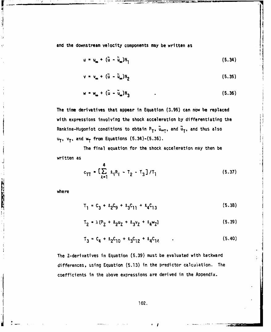
:I)I

and the downstream velocity components may be written as -

U u. + (u N (5.34)1

i

v- v" + (u- u.)N2 (5.35)

W w.w + (u - u.)N3 (5.36)

The time derivatives that appear in Equation (3.95) can now be replaced

with expressions involving the shock acceleration by differentiating the

Rankine-Hugoniot conditions to obtain PT' ULT, and ;T' and thus also

uT, vT, and wT from Equations (5.34)-(5.36). 4

The final equation for the shock acceleration may then be

written as

CTT - iR - T2 - T3 I/T, (5.37) 1where I - C3 + i.2C9 + z3Cii + I 4C1 3 (5.38)

T= )Pz + I 2Uz + i 3vz + •4wz] (5.39)

T3= C4 + 12CIO + 13C12 + 14C14 (5.40)

The Z-derivatives in Equation (5.39) must be evaluated with backward

differences, using Equation (5.13) in the predictor calcuiation. The

coefficients in the above expressions are derived in the Appendix.

102.

[i-i

In the predictor stage. Equation (5.37) can be integrated

to yield

C k + CT" AT (5.41)

- k ck AT (5.42)

The final values of the shock speed and position are obtained in the

corrector stage of the calculation from

ck~ (ck+C + T AT) (5.43)T ~~ TCT +cTTI

ck+l . (ck + + c T) (5.44)f -TOnce the new ehock positions have been determined (predictor

or corrector), the shock slopes c and c6 may be evaluated from

c cy Y (5.45) I.

and

ce = cxX+ CyY 9 (5.46)

where cy and cx are evaluated from difference formulas. At most shock

points, Cy is evaluated at Y = mAY from a standard four point formula as

cy = (Cm.2 - 6Cm_1 + 3cm + 2cm+I)/6AY (5.47)

103.

_ I

At the last two points in each e-plane, the expression

cy - (-2cm. 3 + 9 Cm.2 - l8Cm.l + llcm)/SAY (5.48)

is used, while at the point adjacent to the centerline the form uspd ;s

cy (-2Cm., - 3cm + 6c,,, - Cm+ 2 )/6AY (5.49)

cX is evaluated at X M £X uting the centered two-polr.t difference

formula:

cX = (c+, 1 - c•. 1)/2tx (5.50)

The other shock derivatives required, C•T and ceT, are

determined using the difference formulas given above, but using CT, the

shock velocity, in place of :.

Knowing the shock slopes and velocities, the properties down-

stream of the shock are determined directly from the Rankine-Hugoniot

conditions:

PU p=.U (5.51)

p + pZ2=p •2 (5.52)

h + 1u Z2 h + 2u= (5.53)

For an ideal gas, these equations can be solved analytically for p, p,

and u; for an equilibrium real gas an iterative solution is required.

To avoid this time-.onsuming iteration for real gas calculations, a

table of shock properties as a function of u. is created at the start

104.

I -

of the calculation, thus requiring only interpolation to determine the

downstream properties at any shock point during the computation. Once

II iU has been determined, the downstream velocity components can be computed

from Equations (5.34)-(5.36).

5.5 CENTERLINE POINT TREATMENT

Modifications of the numerical procedures described in the

preceding sections are required for computational grid points located

on the singular centerline. These special procedures required at the

centerline are made necessary by the special forms of the governing

equations derived in Section 3.6, in which the equations at the center-

line are written with terms evaluated only in the planes =0, itf/2, IT,

and 3nr/2.

Within any 4)plane, only forward differences in Y are possible

K ~at the centerline. In order to maintain a two-sided predictor-corrector I4 sequence for the Y-differences at the centerline, terms in the governing

equations are evaluated in the 4=0 and~ = r/2 planes in the predictor

stage, and in the 4)=iT and 4)=3iT/2 planes in the corrector stage. The

resulting numerical scheme thus utilizes information from all directions,

in the spirit of the finite difference scheme used at points not located

r on the centerline.

F At field points along the centerline, the equations to be

solved with this procedure are given by Equations (3.108)-(3.112). A

difficulty arises, however, in the application of this technique when

the coordinate transformation to (C,n,e) space is not axisyrrietric. In

this case, variations in the complex scaling factor g along the center-

line among the 4)planes result 'in the non-correspondence of the

105.

computational grid points in physical space. In other words, even

though the computational grid points at the centerline are equally

spaced in Z for all *planes, grid points with the same Z value in

different planes may represent different points in physical space.

These differences are minimized by the use of the stretching parameterj

a ak in the coordinate transformation defined in Section 3.2, and thus

linear interpolation procedures can be used to resolve the differences

without any noticeable effect on accuracy.

Calculations of the body and shock points along the center-

line do not, of course, experience this difficulty, thus simplifying

the numerical approach at these points. Details on the modifications

required for the characteristic slopes and compatibility conditions at

these boundary points are provided in Section 3.6.

A special procedure is required for the calculation of

4 shock slopes at the centerline, where accuracy requires a formulation

that utilizes information from more than one plane. In particular,

the calculation of c~ in some plane ýl also requires information about

the shock shape from the plane fl + iT. A standard difference procedure

cannot be used, however, when an asymmuetric mapping is invoked; i.e.,

when the mesh spacings tý and the transformed shock locations c are

not necessarily equal in the Ol and Ol + Tr planes.

At the centerline, S = 1 and C=0 for all 4)planes. It

then follows that, with ) denoting the Ol plane and ) 2 denoting

the Ol + Tr plane,

(dnfG)l (dn/G )2 (5.54)

106.

and, in the limit as y÷0,

(de/G) 1 = (dC/G) 2 (5.55)

Using these relations, a four-point difference formula for c• can be

derived for unequally spaced base points;

c =Ac 0 + Bc + Cc 2 +Dc- (5.56)

where

c c (0,-y)

Cl :c(AEI'41)

C2 =c(21l)

cl= co + [c(T 2 ,€l +r) - c(0,fl+ )] GI/G 2

f4 Defining

a = GIAE2/G (5.57)

where A~l and Aý2 are the mesh spacings in the respective * planes, the

coefficients in Equation (5.56) are given by

A = (a-5 + 2)/2At ct(a+l) (5.58)

B = 2/A 1 (a+l) (5.59)

C = -a/2A6l(a+2) (5.60)

D = 2/Agla(a 2 + 3a + 2) (5.61)

107.

The derivative c•T is evaluated at the centerline using the same approach.

For the case of an axisymmetric mapping with a = 1, the difference formula

given by Equation (5.56) reduces to the standard four-point formula given

by Equation (5.47).

Once the solution at a centerline point has been obtained

within any one € plane, the solution within other * planes will also

have been determined. Thermodynamic properties, such as P and s, corre-

spond ,1rectly, but a change in the value of € requires a rotation of

the velocity components. The transfor-ned velocity components within

any € plane can be written in terms of the known components in some

plane @ =€I from

u(ý) = u(ýl)[cospcos~l+ sin~sinfl]

k + w(fb)[sinbcosIi cosbsinbl] (5.62)

v(W) = v(ýi) (5.63)

w(f) - u( 1 )Ecosbsinfl - sin~cosfl]

+ w(ý,)[cos~cosfl + sinbsinfi] (5.64)

Similarly, the shock slope c( at the centerline within any b plane may

be expressed in terms of the slopes in the = 0 and= Tr/2 planes as

c•(€) =c (e=O)coso + c (4=1)sino (5.65)

108.

TIMM'. . .-. 0193. -- -. • -

The transformed centerline shiock velocities may also be related from

the condition that the quantity cT/G, which corresponds to the physical

shock velocity, is the same for all € planes; thus

CT(Y ) G(o)CT(Yl)/G(ol) (5.66)

5.6 CONSERVATION FIELD POINT TREATMENT

The conservation law approach to shock-capturing, described

in Section 4.1, is one of two methods investigated for the calculation

of embedded shocks within inviscid shock layers on reentry vehicle

nosetips. This approach requires the solution of the governing equati:),'s

written in conservation form at all field points using a version of the

MacCormack finite difference scheme described in Section 5.2. After each

integration step, the conservation solution may be damped and smoothed,

as required.

One change has been made in the MacCo-mnack scheme for appli-

cation to the conservation calculations. Because the oscillations inherent

in conservation calculations near a discontinuity arise from approximating

derivatives across the discontinuity, the modification made to the

MacCormack scheme is designed to minimize the number of differences taken

across the discontinuity. This is accomplished by more closely aligning

the numerical domain of dependence of any given field point with the

probable orientation of an embedded shock within the computational mesh.

To illustrate this point, consider the numerical domain of

dependence of a point Y - m&Y and Z = nAZ. Defining the numerical domain

of dependence of a point as all grid points that can effect the solution

at that point in one time step, the standard MacCormack scheme produces

the domain of dependence (in the Y-Z plane) shown in Figure 5.1.

109.

fnl

n

n-i

FIGURE 5.1. NUMERICAL DOMAIN OFDEPENDENCE FOR REGULAR

MACCORMACK SCHEME

Since the V-coordinate direction is nearly normal to the body,

an embedded shock can be expected -co be aligned within the Y-Z mesh as

shown in Figure 5.2. Note that the orientation of the shock in the Y-Z

mesh is counter to that of the numerical domain of dependence for the

regular MacCormack scheme. By changing the orientation of the numerical

domain of dependence to be more consistent with the expected shock

orientation, a smaller portion of the numerical domain of dependence of

a point near the shock will lie across the discontinuity from that point.

*110.

I -/

SHOCK

FIGURE 5.2. TYPICAL ALIGNMENT OF EMBEDDEDSHOCK IN Y-Z COORDINATE MESH

The numerical domain of dependence is reoriented by reversing

the directions of the Z-derivative approximations in the predictor and

corrector stages of the MacCormack scheme; i.e., backward differences

in the predictor stage and forward differences in the corrector stage.

The resulting numerical domain of dependence for this variation on theMacCormack scheme is shown in Figure 5.3.

While this modification to the numerical scheme cannot eliminate

the oscillations inherent in conservation calculations of discontinuities,

it will, in some circumstances, decrease the magnitude of the oscillations.

11l.

*1 I4

n+l

n-i

m-1 m m+l

FIGURE 5.3. NUMERICAL DOMAIN OF

DEPENDENCE FOR MACCORMACK

SCHEME INVERTED IN Z DIRECTION

5.7 X-DIFFERENCING FIELD POINT TREATMENT

The second method examined in this effort for the automatic

calculation of embedded shocks is the X-differencing scheme, described

in Section 4.2. In this approach to the embedded s ock problem, thegoverning equations are written in non-conservation form and certain

terms are written in "split" forms that allow accurate modeling of the

domain of dependence. For example, the term AP, would be approximated

Sas I/2(XZIPZI + Xz2P12) with this scheme, where the particular finite

difference expressions used for PZI and PZ2 would be dependent on the

signs of XZl and XZ2, respectively.

112.

A

In each "split" term, both the ( )1 and ( )2 derivatives

are approximated using a second-order accurate, one-sided, predictor-

corrector finite difference scheme. For either derivative, if the

corresponding coefficient X is positive, backward differences are

employed; coatversely, if the coefficient is negative, forward differences

are used. Backward differences are formed using Equations (5.13) and,

(5.11) in the predictor and corrector stages, respectively, while forward

differences are formed using Equations (5.9) and (5.14), as described

in Section 5.2.

It will be noted in the X-differencing forms of the

governing equations, described in Sections 4.2 (axisymmetric) and 4.4

(three dimensional), that some terms are not split. These unsplit terms

are those that arise from the computational transformation to (X,Y,Z,T)

space and are generally small. The derivatives appearing in these terms

are approximated using convective differences, as described in Section

5.2, maintaining the overall second-order accuracy of the scheme.

113,

i ---. -. 1t

SECTION 6

VALIDATION OF SOLUTIONr•

6.1 LIMITATIONS OF TECHNIQUE

In chis analysis a time-dependent algorithm has been de-

veloped for the computation cf steady inviscid flows over ablated re-

entry vehic!e nosetips with uniform supersonic or hypersonic freestream

conditions. This procedure has been formulated in a new coordinate

system that is capable of being closely aligned with any nosetip geometry,

and includes a technique for the approximate calculation of embedded

shocks. The primary limitation that exists for this technique is the

assumption of isentropic flow downstream of the bow shock.

Be.ause of the inviscid fl.,; assumption, the validity of

this analysis is limited to those high Reynolds number cases where the

thin boundary layer assumption and weak interaction theory apply.

Fortunately, for the flight conditions of reentry vehicles with ablated

nosetios., fcr which this analysis was undertaken, viscous effects are

gen2rally confined to a thin boundary layer adjacent to the vehicle

surface, and the inviscid flow field may be determined independently

of the boundary layer.

This inviscid assumption fails, however, when the nosetip

gecnetry produces separation of the shock layer flow. Prediction of the

separated flow region must include viscous effects, for which the present

analysis is unsuitable.

As discussed in Section 1.0, inviscid theory has been

shown to produce accurate aerodynamic predictions for the flight conditions

of iiterest for all aerodynamic coefficients, with the exception of the

L i 114.

axial force coefficient, which can be significantly affected by viscous

shear and induced pressurq effects. Thus, an inviscid aerodynamic pre-

diction procedure, such as developed here, can be a valuable tool forI

both the pre-flight and post-flight evaluation efforts relating to reentry

vehicle design and performance.

Other limitations apply to the numerical procedure develop.'d

in this research that are commnon to all numerical fluid flow computa-

tional procedures. Fundamentally, it is required for accurate results

that the discrete grid points used in the numerical calculations be

spaced so as to be able to resolve all pertinent features of the body

geometry and the surrounding, flow field. In particular, a finer mesh

will be required in regions of large flow gradients to avoid wiggles in

the numerical solution. (The appearance of wiggles in a numerical solu-

tion is indicative of inadequate mesh resolution for the case being

*computed, or of some other error in the formulation or application of

the numerical technique. This point is discussed more fully by Moretti"2.)

Criteria for the selection of appropriate mesh spacings for an earlier

transonic code were developed by H.11, Kyriss, Truncellito, andMartellci ; these criteria are equally valid for the procedure developed

in this report.

Inconsistencies between the mesh point spacing and flow

gradients can, of course, be eliminated simply by using more mesh points

in the finite difference calculation. More core storage will also be

required for the computer code with an increased number of mesh points;

C the only limitations on the use of this analysis in this regard is the

available core storage on the computer and the economics of a calculation

with a large number of mesh points.

115.

J~--

6.2 CONVERGENCE PROPERTIES

The time-dependent approach to solving the steady transonic

problem is an iterative technique in which advancement of the solution

at any given iteration is defined using the time-dependent equations of

motion. In theory, as time increases to infinity, the steady-state

flow field solution is approached. The time variable used in the time-

dependent technique is directly analogous to the iteration number in

other iterative numerical techniques. In any iterative technique, itii is necessary to define~ criteria for accepting a solution as being con-

verged. This section defines convergence criteria that have been

developed for time-dependent techniques in Reference 4 .These criteria

are defined in terms of fluid dynamic phenomena that arise in the course

of calculating the shock layer about a body in supersonic flow.

The criteria detailed below are sufficient to determine

convergence; i.x., when they are satisfied, the convergence of that

particular solution is ensured. Cases frequently arise, however, when

a satisfactory solution (from the standpoint of accurate aerodynamic

predictions) can be obtained without satisfying all of the convergence

criteria. Acceptance of such solutions requires judgement on the part

* of the user. (In other words, the criteria presented here represent

sufficient, but not necessary, conditions for an acceptable solution.)

For d numerical method to be an accurate solution to a

problem, it must not only converge, but the numerical scheme must be

consistent with the problem being solved. The consistency of the time-

dependent technique used in this analysis is based on its discretization

of the inviscid Euler equations, and its use of non-dissipative

116.

differencing schemes. Thus, the validity of a solution obtained with

this procedure may be examined solely upon the degree of convergence

of the solution (assuming that the mesh spacing selected by the user is

adequate to define the details of the body geometry).

The convergence criteria developed in the previous study

will be summarized below, and then discussed in more detail. These

criteria are:

1. The "stagnation" pressure must have converged

to an essentially constant value. If the actual

stagnation point is known to lie exactly on a

mesh point in the finite-difference grid, the

computed value of stagnation pressure should be

within 0.5% of the known theoretical value of po"

2. The "stand-off distance" of the shock, A0, must

have converged to a constant value.

3. The root-mean-square (rms) of the shock velocities,

(cT/G) , must be converging (decreasing inrms

value) or have converged and, in magnitude, must

satisfy the relation (cT/G)rm 0.004 V0.rms

4. The total enthalpy at every point in the flow

being computed must be within 5% of the known

steady-state total enthalpy.

In a three-dimensional calculation, the flow stagnation

point does not usually correspond exactly to a computational grid point;

thus, for the first two criteria listed above, "Po0" is taken as the

pressure occurring at the centerline body point and "Ao is taken as

the distance between the body point and the bow shock point at

L 117.

'1

the centerline. To illustrate the convergence of these quantities,

Figures 6.1 and 6.2 provide examples of convergent and non-convergent Jtime histories of p0.

In the time-dependent technique an initial shock shape is

assumed and is allowed to adjust its position during the cours2 of the

calculation. Theo.'etically, for a solution that has converged to a

steady state, the shock velocity will have vanished at all shock points

to within some "epsilon" of the freestream velocity. On a more practical

basis, the criterion described above ((c/G) !g 0.004 V.) is sufficient

to determine a satisfactorily converged solution, provided that the

magnitude of (cTG)r is decreasing from step to step (i.e., is not

diverging)when the criterion is only marginally satisfied. Samples of

converging and diverging time-histories of (cT/G)rms are illustrated

in the plots shown in Figures 6.3 and 6.4. One caveat is required

in the assessment of (cT/G) . Since (cT/G) is, in a sense, anrms rms

average of individual shock velocities, it is possible that the critevion

on (cT/G) be satisfied, while one or two individual shock velocities

are relatively large. Thus, judicious assessment of convergence based

on shock velocity should include examination of the individual shock

velocities as well as the value of (cT/G) .

The final criterion for convergence is based upon the

conservation of total enthalpy. Since the total enthalpy is not con-

stant in an unsteady flow. an indication of the convergence and accuracy

of a time-dependent solution can be obtained by examining the difference

between the computed total enthalpy at each point and the known steady

state value (which is equal to the freestream total enthalpy).

•,' . . . -" . . •i

THEORETICAL•8 ~VALUE

+ .1

;V)sV)

• .. . . ..I I

STIME

FIGURE 6.1. TYPICAL POT HISTORY (CONVERGED)

119

Ilg

TIME_

TIME

FIGURE 6.2. TYPICAL P 0 HISTORY (NOT CONERGED)CA

TIME

10,1I0

C>)

I o-

T10-I

-J .

1 • 10- II -

TIME

FIGURE 6.3. TYPICAL (CT/G)ms HISTORY (CONVERGED)

121.

- .- -- --- - . _ _ _ _ _ _ _ _ _ .. . . .. ... _ _,.-_- _ _ _, _ _ _-_" _ _ _ _ __,,__._._I

lol-

10

CoI

10

TIME

FIGURE 6.4, TYPICAL (CT/G)rm HISTORY (NOT CONVERGED)

122.

Defining

AH= (H-H.)/H•, (6.1)

a suitable criterion for convergence has been found to be

LAHI i 0.05 . (6.2)

The question of convergence of the time-depenideov; solution

can be summarized as follows: when a time-dependent solution satisfies

the convergence criteria described above, it can be used with confidence

to provide accurate and reliable aerodynamic predictions, provided that

the mesh adequately resolves the important details of the body geometry

and of the surrounding flow field.

6.3 VALIDATION OF NOSETIP SOLUTION

In this section the numerical procedures developed in this

research are validated by comparisons of predictions to experimental data

and, where appropriate, predictions obtained with other numerical tech-

niques. The validation process described in this section pertains only

to the nosetip solution procedures; the ability of these transonic

procedures, when coupled to a steady supersonic afterbody code, to make

accurate determinations of total vehicle inviscid aerodynamics is

demonstrated in Section 6.4.

Two versions of the three-dimensional time-dependent

inviscid code formulated in the new coordinate qystem (based on a series

of conformal transformations) have been developed in this effort. The

basic version, which is denoted by CM3DT(NC), is formulated in terms of

the non-conservation dependent variables and is incapable of treating

123.

embedded shocks. The version based on the X-differencing scheme,

providing a method for treating embedded shocks, is denoted by CM3DT(X). •I

The first step in the validation process is the demonstra-

tion of the ability of the new coordinate system to permit accurate

calculations of the inviscid flow over a wide variety of body shapes,

including shapes that could not previously be treated with transonic 4

codes formulated in standard coordinate systems (e.g., spherical). Use

of this new coordinate system does not, however, reduce the accuracy of

calculations for shapes that are well-suited to analysis using a standard A

coordinate system. VTo illustrate the ability of the new coordinate system to

treat shapes that are well-suited to calculations using a standardVcoordinate system, Figures 6.5 and 6.6 present predictions of the bow

shock shape and surface pressure distribution for a sphere in equilibrium

air at an altitude of 100 KFT with a freestream velocity of 20,000 ft/sec.

STwo predictions are made with the CM3DT(NC) technique, using both a

coarse mesh (6 x 9; i.e., six points across the shock layer and nine

points along the body) and a fine mesh (11 x 17). The other predictions

shown for this flow have been obtained from the inverse technique of

Lomax and Inouye 3 3 and from the technique developed by Kyriss end

Harris 8 , which is an explicit time-dependent finite-difference code

formulated in a spherical coordinate system. (The method of Kyriss and

Harris has been extensively validated by comparisons to experimental

data, e.g., by Hall, Kyriss, Truncellito, and Martellucci 4 and by

Hall and Nowlan 5 .)

124.

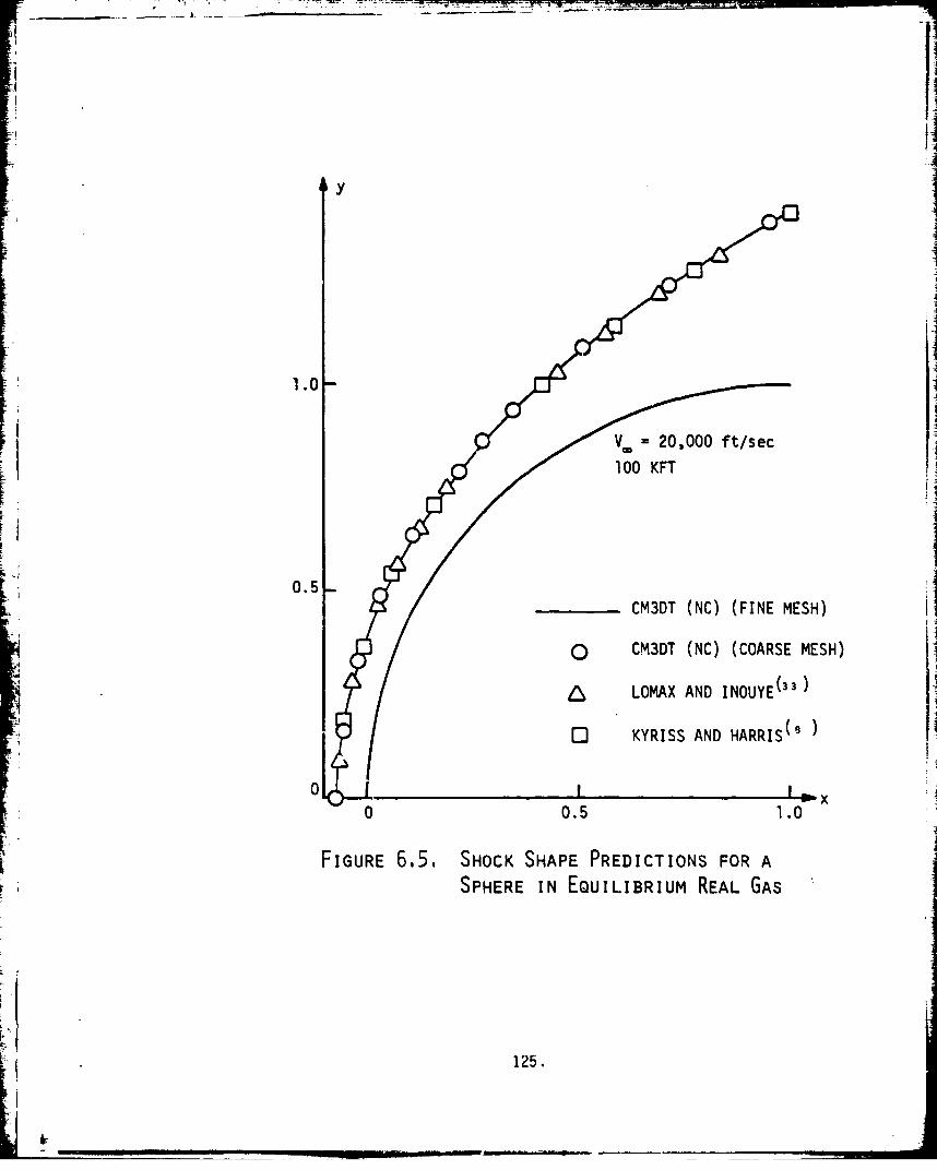
;i

y

1.0-

I

V --20,000 ft/sec

1;O0 KFT

0.5

CM3DT (NC) (FINE MESH)

0 CM3DT (NC) (COARSE MESH)

LOMAX AND INOUYE(33)

0 KYRISS AND HARRIS(s

0 II x

0 0.5 1.0

FIGURE 6.5. SHOCK SHAPE PREDICTIONS FOR ASPHERE IN EQUILIBRIUM REAL GAS

125.

I v _.n

.. u m l lm tl m w. .fJ.•,.,,• ..- • * ..

- ~w-y-LLI

LUI

LA0 LWrV) %'

LAJ 9z LwzwL6 C-)-

z

LJ -i

z CQI- 0 0

Im L) 0

I4- a: U

LL0126

i = .. -,, /••• • • -• •• r . T __ _ __ _ __ _ __ _ - a •

Li

The results obtained with the C?¶3DT(NC) code show

excellent agreement with the other predictions for this case and,

furthermore, are also seen to be invariant with refinement of the mesh,

verifying the consistency of the numerical approximations. This case

also serves to illustrate the real gas thermodynamic capabilities of

the CM3DT procedure.

The ability of the new coordinate system to treat less

regular shapes is shown in Figures 6.7-6.10, which present comparisons

of bow shock shape and surface pressure distribution predictions for

the axisymmetric PANT Triconic (described by Jackson and Baker in

Reference 21) to experimental data at M. = 5 and a = 00. (Although

an indented shape, no embedded shock forms on this configuration at

these flow conditions.) Figure 6.7 presents the surface pressure distri-

bution predicted with the CM3DT(NC) procedure for this configuration,

which has a small radius corner at the shoulder leading back to an aft

cone, as evident in Figure 6.10. The agreement between the prediction

and the data is seen to be good in Figure 6.7, except for oscillations

arising in the vicinity of the corner. These oscillations are the result

of inadequate resolution of the finite difference grid in the vicinity

of the corner, as discussed and illustrated by Hall, Kyriss, Truncellito,

and Martellucci'; . The influence of this sharp corner is made more

evident by, the results obtained from a similar calculation, in which

the sharp corner and cone were removed. As shown in Figure 6.8, no

oscillations appear in the CM3DT(.NC) prediction of surface pressure when

the sharp corner is eliminated.

127.

Li

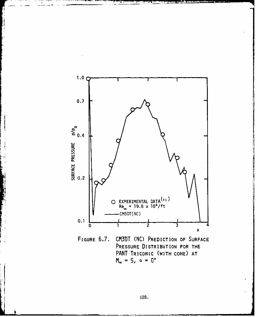
1"°C-- --~ -I ----- ----. - - " i.-~.a-

1.0

0.7

0.4

Lu

tA

Lu

40.2

0 EXPERIMENTAL DATA(21)

Re = 19.8 x 106 /ft

i CM3DT(NC)

0.10 1 2 3 4

FIGURE 6.7. CM3DT (NC) PREDICTION OF SURFACEPRESSURE DISTRIBUTION FOR THE

PANT TRICONIC (WITH CONE) AT

M= 5, e=00

128.

0.7

0.4

0.2

SEXPERIMENTAL DT(1Re.,= 19.8 x 1 6 f

CM3DT(NC)

0.1

0 1 2 34X

SFIGURE 6.8. CM3DT (NO) PREDICTION OF SURFACE

PRESSURE DISTRIBUTION FOR THE PANTTRICONIC (WITHOUT' CONE) AT =,=5.,

0 0-

129.

-1

1-1

IFA 1.1

0.7

§C . 4

Lu 0.4

0.2

0 EXPERIMENTAL DATA(21)

Re. = 19.8 x 106/ft

CM3DT(\)

0.1 I I I0 1 2 3 4

x

FIGURE 6,9. CLi3DT (M) PREDICTION OF SURFACE

PRESSURE DISTRIBUTION FOR THE PANTTRICONIC (WITH CONE) AT Mo = 5, a = 0

130.

rif

-j-

CII

ItE

U.1

00

I-, u 4

E~oA!U ti.

LULJ

It was discovered during the course of this research that

the X-differencing scheme, in addition to its shock-capturing capability,

has the additional ability of eliminating the spurious oscillations that

arise at such sharp corners. This capability is illustrated in Figure

6.9, which depicts the surface pressure distribution for the PANT Triconic

(with the sharp corner and conical aft section included) as predicted

by the CM3DT(M) procedure. The lack of oscillations in this calculation

is a manifestation of the ability of the X-differencing scheme to

accurately model the physical domain of dependence, preventing oscillations

from propagating upstream in supersonic flow.

The final comparison for the PANT Triconic predictions

is shown in Figure 6.10, demonstrating the agreement between predictions

and experimental data for the bow snock shape. (All CM3DT predictions,

both with and without the sharp corner, for the bow shock shape are

essentially equivalent.)

It should be noted that attempts at computing this slender

shape with the technique of Kyriss and Harris e , which is formulated in

a spherical coordinate system, were unsuccessful, because of the inabilityof the spherical coordinate system to be closely alignefi with the body

geometry.

Further evidence of the abilities of the new coordinate

system is provided in Figure 6.11, which presents a comparison of surface

pressure predictions and experimental data for the PANT Simple Biconic

(described by Jackson and Baker 21 ) at 5= and a = 50. This axisym-

metric configuration is a 450 sphere-cone nosetip, with a rounded

shoulder leading to a 60 aft cone. As seen in this figure, the

132.

0.7

0.4

EXPERIMENTAL DATA(21)0.2 Rec, = 18.4 x 106/ft

Lu 0 LEE PLANEL 0L

0 WIND PLANE

Ln

0.1 0____CM3DT (NC)

1 - - -KYRISS AND HARRIS~0.07

0.040 12

xFI-GURE 6.11, SURFACE PRESSURE PREDICTIONS FOR THEI

PANT SIMPLE BiCONIC AT Moo= 5, =5*

133.

II

predictions of both CM3DT(NC) and the technique of Kyriss and Harris8

show good agreement with the data, except for the oscillations created

by the lack of adequate resolution at the shoulder. Not apparent from

this figure, however, is the improved convergence behavior obtained

with the new transonic technique. After 400 time steps, using the

same number of grid points, and computing approximately the same elapsed

physical time, the root-mean-squares of the shock velocities, which,

as discussed in Section 6.2, are reliable indicators of convergence,

differ by an order of magnitude. For CM3DT(NC), (CT/G)c/V = 0.004,

while the equivalent quantity for the other technique is 0.056, which

does not satisfy the convergence criterion.

Another good indicator of convergence for a time-dependent

technique is the maximum error in computed total enthalpy. For CM3DTCNC),

the maximum error is 8.6% for this case, compared to a maximum error of

28.5% for the technique of Kyriss and Harris, further illustrating the

benefits of the new coordinate system.

The ability of the CM3DT(NC) code to treat asymmetric shapes

at angle of attack using the new coordinate system is illustrated in

Figure 6.12, showing predictions of the bow shock shape for the Blunt-l

shape at M = 13.4 and a = 30. (This asymmetric nosetip shape was

derived in a nosetip reconstruction analysis described by Hall and

Nowlan' .) The predicted shock shape is seen to agree well with that

predicted using the technique of Kyriss and Harris 8

The final step in the validation process for the nosetip

solution is the demonstration of the ability of the CH3DTCX) procedure

to predict flows over shapes that produce an embedded shock. In Figure

I 134.

CM3DT(.NC)

KYRISS AND HARRIS 8

FIGURE 6.12. Bow SHOCK SHAPE PREDICTIONS FOR THEhi ~THE BLUNT-i SHAPE AT MD=13.4, =30

135.

6.13, a comparison is shown of the predicted surface pressure distri-

bution and the experimental data for the PANT Triconic at M = 5 and

a 100; the agreement is seen to be excellent. Schlieren photographs

of this configuration at this angle of attack, which may be found in

Reference 21, clearly indicate the presence of an embedded shock in

the lee plane. This comparison serves to illustrate the capability of

the three dimensional version of the X-differencing scheme to compute

inviscid nosetip flow fields with embedded shocks. (The capabilities of

the axisymmetric version of the X-differencing scheme have been demon-

strated in Section 4.)

6.4 PREDICTION OF TOTAL VEHICLE INVISCID AERODYNAMICS

In the preceding section the ability of the CM3DT technique to

accurately predict inviscid flow fields over ablated reentry vehicle

nosetips has been demonstrated. To complete the validation prucess for

this technique, it remains only to demonstrate the capability of the

CM3DT nosetip code, when coupled with an existing supersonic afterbody

code, to make accurate predictions of total vehicle inviscid aerodynamics.

For this validation effort, the CM3DT code has been coupled to the super-

sonic afterbody code of Kyriss and Harris 8 , which is a steady, fcrward

marching finite difference technique formulated in a cylindrical co-

ordinate system. (Coupling of the nosetip and afterbody codes requires

interpolation on the nosetip solution to determine the flow variables

in the initial data plane of the afterbody solution and an integration

to determine the forces and moments acting on the nosetip.)

136.

b,1

1.0

0.7

VVK ~~?o.4

: . EXEIETLDT(I

•0.2 Re = :19.9 x 106 /ft

k 0 WIND PLANE

.1 -0 CM3DT ( 2)

EXEIMNA DAT

01 2

x

FIGURE 6.13. SURFACE PRESSURE PREDICTIONS FOR THEPANT TRICONIC AT Mo = 5 a = 100

137.

In the calculation of total vehicle aerodynamics it is of

critical importance to accurately model the influence of the nosetip

shape on the afterbody flow field, dnd thus on the resulting forces

and moments acting on the vehicle. For example, the importance of

the downstream influence of an asymmetric nosetip in the determination

of the trim angle of attack (aT) for a ballistic reentry vehicle has

been demonstrated by Hall and Nowlan 5 . Direct coupling of numerical

flow field calculations for nosetips with afterbody procedures will

automatically include the nosetip's influence on the afterbody flow

field.

The first validation case for the CM3DT code coupled to the

afterbody solution is presented in Figure 6.14. This figure depicts a

comparison of predictions of the normal force coefficient (CN) and the

pitching moment coefficient (C m) as a function of angle of attack for

a 90 cone with a spherical nose, with a vehicle bluntness ratio (RN/RB)

of 15%, at M= 20 in ideal gas (y = 1.4) with no sideslip (a = 00).

The prediction labeled CM3DT was obtained using the CM3DT(NC) code to

pr-ovide the initial data required for the Kyriss and Harris 8 after-

body code; the other prediction was obtained using an axisymmetric

calculation of the spherical nosetip flow field (in wind-fixed coordi-

nates), with the required initial data being obtained by suitable rotations

of the spherical solution, as described in Reference 8 . The accuracy

of the Kyriss and Harris afterbody code, and of the Kyriss and Harris

axisymmetric and three-dimensional transonic codes for blunt, convex

nosetips, has been extensively demonstrated through comparisons of

predictions to wind tunnel data, as shown, for example, in References

138.

0.4 I

CM3DT(NC)

0.3 KYRISS AND -RIS

C>wU 0.2

0.1

0.

0

4 1 ~-50.1"Z•L

uJ -

U.S{. -0.2

-" Xcg/LA 0

-0.3 I I I I I0 2 4 6 8 10

ANGLE OF ATTACK (DEG.)

FIGURE 6.14. NORMAL FORCE AND PITCHING MOMENTCOEFFICIENTS VS. ANGLE OF ATTACK FOR

9" SPHERE-CONE OF 15% BLUNTNESS AT

tM. = 20, *=O"

139.

4 , 5 , and 8. As is evident in Figure 6.14, the agreement between

the predictions of CN(a) and Cm(a) is excellent.

The comparison of aerodynamic predictions for spherically

blunted cones obtained with these two techniques is continued in Figure

6.15. This figure illustrates the excellent agreement obtained between

the two predictions of pitch center of pressure as a function of

bluntness ratio for the 90 sphere-cone at M= = 20 and oL - 50. (The

pitch center of pressure is defined as Xcp/LA z Xcg/LA - Cm/CN when

the reference length used in the non-dimensionalization of the pitching

moment is the virtual cone length.)

The ability of CM3DT to provide accurate initial data to

the afterbody calculation for spherically-nosed vehicles is further

demonstrated in Figure 6.16. This comparison is similar to that shown

in Figure 6.14, in that predictions are obtained for CN(c) and Cm(a)

for a 15% blunt 90 sphere-cone at M 20, except that the vehicle is

at k onstant sideslip angle (a) of 50. The agreement between the two

predictions is again seen to be excellent, and serves to verify the

ability of the CM3DT to compute flow fields on nosetips in both pitch

and yaw.

Figures 6.17 and 6.18 present a comparison of inviscid aerodynamic

prP- c'ons ained for a vehicle with a blunt asymmetric nosetip. The

vehicle is a 60 cone with a nominal bluntness ratio of 25%; the nosetip

is the Blunt-1 shape (illustrated in Figure 6.12), which was derived in

a nosetip sh- .econstruction effort described by Hall and Nowlan.

(In Reference 5 , the Blunt-1 shape was selected as a plausible nosetip

shape for an actual flight vehicle at 20 KFT, based on actual recession

140.

-- n

inILLIzI

00 (nLUw

U- 0CD

k t ui C-

VnLV) LU 0

o =

U,"

a-4;

4. 0o Z

L3 C; C; 6

I/ -

HnS' AONR3 HI

141.

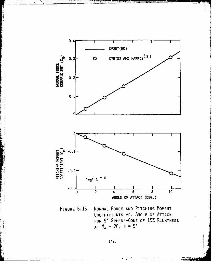
0.4CM3DT(NC)

L) 0.30 KYRISS AND HARRIS

ccLL.~

0.2Ul.,h

0000.1

III J

CD

A -.

, • , = - c g / L A = 0

ZL, -0.31 1 1 1 I

S0 2 4 6 8 10

i ANGLE OF ATTACK (DEG.)

4

FIGURE 6.16. NORMAL FORCE AND PITCHING MOMENTCOEFFICIENTS vs. ANGI.E OF ATTACKFOR 9° SPHERE-CONE OF 151% BLUNTNESS

"I AT M.."' 20, 0 = *

S142.

I0.121

CM3DT(NC)

0 HALL AND NOWLAN(5)

E 0.08 0 1Lh.

I-

S0.04

0

0 13 4 5

ANGLE OF ATTACK (DEG.)

FIGURE 6.17. NORMAL FORCE COEFFICIENT VS, ANGLE

OF ATTACK FOR BLUNT-i CONFIGURATION

AT MW = 13.4, 20 KFT ALTITUDE

143.

0. 008

S0.004•

L•JL. Xcg/LA = =0.5886 0

LaJ 0

.- " CM3DT(NC)S-0.004-

0 HALL AND NOWLAN( 5)SMAGNETOMETER a

-0.008 I I0 2 3 45

ANGLE OF ATTACK (DEG.)

FIGURE 6.18. PITCHING MOMENT COEFFICIENT VS, ANGLEOF ATTACK FOR BLUNT-i CONFIGURATION

AT MW = 13.4, 20 KFT ALTITUDE

1 144.

measurements and on the consistency of aerodynamic characteristics derived

from motion data with those computed with the transonic nosetip and

supersonic afterbody codes of Kyriss and Harris 8 . The computed trim

angle of attack, aT = 3.35', was consistent with that measured by an

onboard magnetometer, as indicated in Figure 6.18.)

A comparison of CN(a) predictions for this configuration is

presented in Figure 6.17, and fair agreement is evident between the

predictions obtained with the CM3DT(NC) technique and with the three-

dimensional transonic code of Kyriss and Harris. Similar agreement is

seen in the Cm(c() predictions shown in Figure 6.18. The CM3DT pre-

dictions indicate a trim angle of attack of 3.580, which is within the

aT range measured by the magnetometer.

The above comparisons have demonstrated the ability of the

CM3DT code to produce nosetip flow field solutions and afterbody solution

initial data for spherical and blunt convex nosetip shapes with an accuracy

equivalent to that of the extensively valioated cransonic technique of

Kyriss and Harris 8 . Because the CM3DT code has been developed to

extend the range of nosetip geometries for which accurate numerical

inviscid aerodynamic predictions can be made, however, the remaining

validation cases to be documented in this section must rely on compari-

sons of CM3DT solutions with wind tunnel data for complete reentry

vehicles, rather than with other numerical solutions.

The first case to be considered in this comparison of numerical

predictions and experimental data is the N8 nosetip, shown in Figure

6.19, mounted on a 6.30 cone, with a nominal bluntness of 25%.

145.

L.,

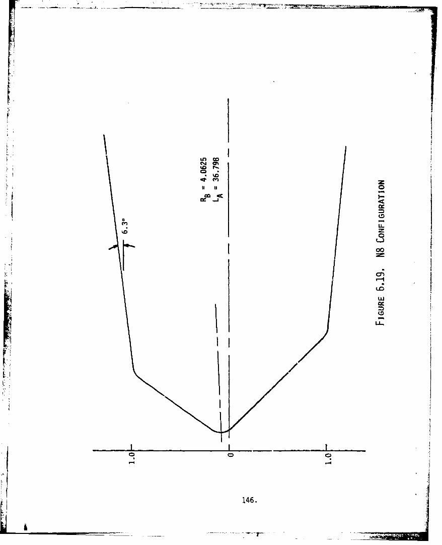
un ii.0

Ci-

%00

00

0m

L6

146.

Experimental data were obtained at Mach 8 in Tunnel B at the Arnold

Engineering Development Center (AEDC); details of the tests and the•ii

resulting data are described by Hahn and Little". The N8 nosetip is

a "tilted cone" shape, with relatively small shoulder radii, and is

intended to simulate an asymmetric shape that could result from

turbulent ablation on the nose. Because of the fairly sharp corners

on this shape, the CM3DT(X) code was used to generate the nosetip flow

field solution, since the X-differencing scheme has been found to

eliminate wiggles arising at sharp corners, as discussed in Section 6.3.

Comparisons of the predictions of the normal force and pitching

moment coefficients to the experimental data are shown in Figures 6.20

and 6.21, respectively. These comparisons show good agreement between

the predictions and the data. Also, the CM3DT technique has accurately

computed the trim angle of attack to be 3.860 (based on a linear inter-

polation between values of Cm computed at a = 20 and a = 40), compared

to the experimentally determined value of 3.520 (based on a linear

interpolation between-data points at a = 30 and a = 40).

The final validation cases to be presented in this section

involve comparisons between predictions and tunnel measurements of

aerodynamic forces and moments for a 6° cone (25% nominal bluntness)

with two axisymmetric indented nosetips. The tests were conducted in

Tunnel F at AEDC at a Mach number of 11.6 and are described by Boudreau,

Crain, and Edenfield 35 The nosetips tested were the Very Mildly In-

dented Body (VMIB) and the Mildly Indented Body (MIB), described by

Reeves, Todisco, Lin, and Pallone 20 , and illustrated in Figures 4.4

and 4.7, respectively.

147.

LL.

w-UD

c(0 z~oo

0L *D w <C- 0 J u z

0. 8 cl LL. '

L~~JC CD) Li

-LJ LL

c..J 00 I

~LL

CNJ

0I I '.0LL-

0o 0) 00 0D

(NO) IN3IOIdJO30 30HOA IVRdON

148.

CAl

LU

-J 4-)

4- iLu - u. LU~

UJl 9 5L-) F-W

0..L 8 (DU

LUL

CID z

o ___ _ 011ouLOUo~

CL-. LL .

0 '.0

I--J I I

( ) INHI3UJJO INJWOW SNIHOJ.d

149.

Since both the VMIB and MIB nosetips are indented and testn were

conducted at non-zero angles of attack, it was necessary to use the

CM3DT()) code because of the shock-capturing capability of the X-dif-

ferencing scheme for the treatment of embedded shocks. Figures 6.22 and

6.23 present comparisons of CN(c) and Cm(a) predictions to the data,

respectively, for the VMIB nosetip, and the agreement is seen to be

excellent.

The same comparisons are presented in Figures 6.24 and 6.25 for

the vehicle with the MIB nosetip. Again, the overall agreement between

the predictions and the data is seen to be good. (Discrepancies are

apparent, however, between the predicted and measured values of CN and Cmat a = 40 for this configuration. The validity of the CM3DT calculation

at this angle of attack, as measured by the convergence of the computation,

is comparable to that of the calculations at other angles of attack, where

good agreement between predictions and data is evident.)

Further validation of the VMIB and MIB calculations is presented

in Figure 6.26, which depicts the predicted pitch center of pressure loca-

tions compared to the experimental center of pressure ata presented in

Reference 8. The agreement is seen to be excellent.

In conclusion, the ability of the CM3DT(A) code to compute in-

viscid flow fields on indented nosetips at angle of attack, when coupled

with a supersonic afterbody code, has resulted in a technique that is

capable of producing accurate aerodynamic predictions for reentry vehicles

with realistic ablated nosetip shapes, as demonstrated above. This capa-

bility represents a significant extension of the applicability of numerical

techniques to the evaluation of reentry vehicle inviscid aerodynamics.

150.

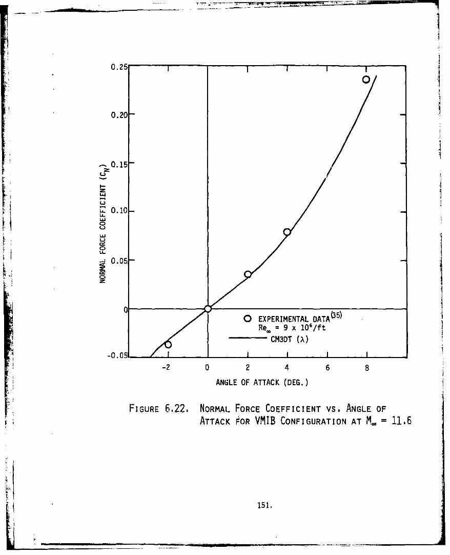
0.25

0.205

--. 0.15/

EO.1O-LiJ

0

Re. = 9 01•

K-2 0 2 40

•i ANGLE OF ATTACK (DEG.)

FIGURE 6.22, NORMAL FORCE COEFFICIENT VS. ANGLE OF

ATTACK FOR VMIB CONFIGURATION AT M0a = 11.6

151.

0.02

LU ,

0.

-0.02

-0.04IlI

cg

-2 0 2 4 6 8

ANGLE OF ATTACK (DEG.)

FIGURE 6.23. PITCHING MOMENT COEFFICIENT VS. ANGLEOF ATTACK FOR VMIB CONFIGURATION AT

MC= 11.6

152.

0.25

0.20-

0o.15

S0.0

0

0Re 0.1010/f

.oo• /9 .

-0.051

-2 0 2 4 6 8

ANGLE OF ATTACK (DEG.)

FIGURE 6.24, NORMAL FORCE COEFFICIENT VS. ANGLE OF

ATTACK FOR MIB CONFIGURATION AT Tt 11.6

153.

LL

0.0

• 0 EXPERIMENTAL DATA('35)1Re., -9 x 106/ft..

-- CM3DT (,

E

S-0.02_

•-I-a-0.

-2 0 2 4 6 8

ANGLE OF ATTACK (DEG.)

4 FIGURE 6,25. PITCHING MOMENT COEFFICIENT VS. ANGLE

OF ATTACK FOR MIB CONFIGURATION AT Mi = 11.6

jtl 154.

0.75

. 0.70

"A 0 VMIBo 0"0 [0 DATA 5)

• 0 - MIB

VMIB

CM3DT(X) 1 . MIB0.65 I I I I I

-2 0 2 4 6 8

ANGLE OF ATTACK (DEG.)

FIGURE 6.26, PITCH CENTER OF PRESSURE VS. ANGLE OF

ATTACK FOR VMIB AND MIB CONFIGURATIONS

AT Mo = 11.6

155.

SECTION 7

CONCLUSIONS 1

The goal of this research effort has been the development of -

a computational technique for the prediction of inviscid flow fields

about ablated reentry vehicle nosetips. The development of this capa-

bility has required the elimination of two major deficiencies in

existing supersonic blunt body flow field procedures. First, a co-

ordinate system h.; been developed that is capable of being closelyF aligned with ablated nosetip shapes, producing coordinate surfaces

that are either nearly parallel or nearly normal to the nosetip surface.

Second, an approximate capability has been developed for the calcula-

tion of embedded shocks on indented nosetips.

The new three-dimensional coordinate system is based on

sequences of conformal transformations that are carried out independently

in each meridional plane. The conformal transformations developed for

this effort are defined in terms of "'hinge points", which are discrete

points selected such that the body contours are modeled in an approxi-

mate manner.

A three-dimensional blunt body code has been developed using

this new coordinate system, with the governing equations written in

non-conservation form. A second-order accurate, explicit procedure

has beens used to integrate the time-dependent equations, with the

steady state solution being sought as the asymptotic limit of an

unsteady flow. Body points and bow shock points are computed using

special algorithms that are based on the method of characteristics.

156.

This new three-dimensional blunt body code has extended the

range of nosetip geometries for which inviscid flows can be success-

fully computed. For ablated nosetips without embedded shocks, this

technique has demonstrated excellent agreement with experimental data

and (for sufficiently regular shapes) with other numerical techniques.

As a first step in treating the embedded shock problem on

Aablated nosetips, two shock-capturing techniques have been examined

for the axisymmetric problem. These two procedures, the conservation

formulation and the X-differencing approach, can only approximate

discrete embedded shocks, but do not require special logic to detect

the embedded shocks or to treat their movement through the coordinate

mesh during the time-dependent calculation. Comparisons of these two

techniques have been carried out by developing two axisymmetric time-

dependent blunt body codes, using the new coordinate system developed

in the first part of this effort.

The conservation formulation, in which the dependent variables

used are derived from the integral conservation laws, was found toLA

require numerical damping to control the oscillations produced when

capturing a shock. This artificial damping has been demonstrated to

have the potential of distorting the shock layer being computed,

leading to smooth but inaccurate results.

In the X-differencing approach, in which the non-conservation

form of the governing equations is solved using a finite difference

scheme that accurately models the domain of dependence of each mesh

point, no numerical damping was required. In general, the X-differencing

scheme has been found to produce better agreement with experimental data

for nosetips with embedded shocks than the conservation approach.

157.

The X-differencing scheme is at best, however, an approximate embedded

shock solution, since there is no mechanism for an increase in entropy

across the "captured" embedded shock.

Based on this comparison of axisymmetric shock-capturing

techniques, the X-differencing scheme was selected for extension to

the three-dimensional problem, using the new coordinate system. (This

effort is the first use of the X-differencing scheme for a three-

dimensional, time-dependent problem.) The three-dimensional X-differencing

scheme has produced good agreement with experimental data for indented

nosetips at angle of attack.

In addition to its shock-capturing abilities, the X-differencing

scheme has also demonstrated an ability to eliminate oscillations that

appear in other blunt body solutions at sharp corners in supersonic flow.

This capability arises from the accurate modeling of the domain of

dependence of each grid point by the X-differencing scheme, preventing

disturbances from propagating upstream in supersonic flow. The capa-

bilities of the X-differencing scheme are evidence of the importance

of considering the physics of the flow when developing a numerical

simulation.

The codes developed in this effort have significantly in-

creased the range of ablated nosetip geometries for which inviscid

aerodynamic predictions can be obtained. Coupling these nosetip codes

to an existing supersonic afterbody code has provided a unique capa-

bility for the determination of inviscid aerodynamic performance

for an entire reentry vehicle, both for pre-flight aerodynamic

predictions .nd for post-flight performance analyses. The utility

of these codes is enhanced by their relative efficiency, with a

158.

I

typical nosetip flow field calculation requiring approximately three

minutes on the CDC Cyber 176 computer, allowing the use of these

codes on a routine basis for design and evaluation efforts.

Extension of the current effort would require the develop-

ment of a procedure for treating embedded shocks as discrete dis-

continuities. Such a shock-fitting technique, in which the Rankine-

Hugoniot conditions are strictly enforced across the embedded shocks,

would remove the approximations inherent in the isentropic X-differencing

scheme. The development of a shock-fitting algorithm will be simplified

by the use of the X-differencing scheme since the X-scheme provides

a convenient, reliable method for the detection of shocks. Coupled

with the generalized coordinate system developed in this effort, a

shock-fitting technique would represent the ultimate capability forflow field predictions for ablated reentry vehicle nosetips, subject to

the limitations inherent in the assumption of inviscid flow.

A

159.

a j

_ , -- -,-l -. •

SECTION 8

REFERENCES

1. Dirling, R. B., Jr., "Asymmetric Nosetip Shape Change DuringAtmospheric Entry," AIAA Paper No. 77-779, June, 1977.

A

2. Pettus, J. J., Larmour, R. A., and Palmer, R. 1., "A PhenomenologicalFramework for Reentry Dispersion Source Modeling," AIAA Paper 77-1152,August, 1977.

3. Hayes, W. D. and Probstein, R. F., Hypersonic FZow Theory, 1stedition, Academic Press, New York, 1959. A

4. Hall, D. W., Kyriss, C. L., Truncellito, N. T., and Martellucci, A.,"Nose Trim Study, Volume II. An Evaluation of the G.E. Three-Dimensional Flow Field Program for Ballistic Reentry Vehicles withAsymnmetric Noses," SAMSO TR-77-46, September, 1976.

5. Hall, D. W. and Nowlan, D. T., "Aerodynamics of Ballistic ReentryVehicles with Asymmetric Nosetips," J. Spacecraft and Rockets, 15,1, 55-61, Jan.-Feb., 1978.

6. Moretti, G. and Salas, M., "The Blunt Body Problem for a ViscousRarefied Gas Flow," AIAA Paper 69-139, January, 1969.

'. MacCormack, R. W., "The Effect of Viscosity in Hypervelocity ImpactCratering," AIAA Paper 69-354, January, 1969.

' 'I

8. Kyriss, C. L. and Harris, T. B., "A Three-Dimensional Flow FieldComputer Program for Maneuvering and Ballistic Reentry Vehicles,"presented at the 10th USN Aeroballistics Symposium, July, 1975.

A 9. Moretti, G. and Pandolfi, M., "Entropy Layers," Polytechnic Instituteof Brooklyn, PIBAL Report 71-33, November, 1971.

10. Kutler, P., Reinhardt, W. A., and Warming, R. F., "NumericalComputation of Multi-Shocked, Three-Dimensional Supersonic FlowFields with Real Gas Effects," AIAA J., 11, 5, 657-664, May, 1973.

11. Marconi, F., Salas, M., and Yaeger, L., "Development of a ComputerCode for Calculating the Steady Super/Hypersonic Inviscid FlowAround Real Configurations. Volume I - Computational Technique,"NASA CR-2675, April, 1976.

12. Solomon, J. M., Ciment, M., Ferguson, R. E., Bell, J. B., Wardlaw,A. B., Jr., "A Program for Computing Steady Inviscid Three-DimensionalSupersonic Flow on Reentry Vehicles, Volume I: Analysis andProgramming," NSWC/WOL/TR 77-28, February, 1977.

13. Kentzer, C. P., "Discretization of Boundary Conditions on MovingDiscontinuities," Second Irternational Conference on NumericalMethods in Fluid Dynamics, University of California, Berkeley,

* ISeptember 15-19, 1970.

160.

'1 _ _ _ _ _-

1< i

14. Hall, D. W., "The Influence of Boundary Point Procedures onAccuracy and Efficiency in Flow Field Calculations," General ElectricCo., TIS 77SDR016, March, 1977.

15. Moretti, G., "Calculation of the Three-Dimensional, Supersonic,Inviscid, Steady Flow Past an Arrow-Winged Airframe," PolytechniciInstitute of New York, POLY-AE/AM Report No. 76-8, May, 1976. A

16. Moretti, G., "Conformal Mappings for Computations of Steady, Three-Dimensional, Supersonic Flows," Numerical/Laboratory Computer Methodsin Fluid Mechanics, ed. A. A. Pouring and V. I. Shah, ASME, NewYork, 1976.

17. Moretti, G., "Computation of Shock Layers about Ablated, Blunt-Nosed Bodies," Polytechnic Institute of New York, POLY-M/AE ReportNo. 77-14, August, 1977.

18. Kutler, P., Chakravarthy, S., and Lombard, C., "Supersonic Flowover Ablated Nosetips Using an Unsteady, Implicit NumericalProcedure," AIAA Paper 78-213, January, 1978.

19. Moretti, G., "An Old Integration Scheme for Compressible FlowRevisited, Refurbished, and Put to Work," Polytechnic Instituteof New York, POLY-M/AE Report No. 78-22, September, 1978.

20. Reeves, B. L., Todisco, A., Lin, T. C., and Pallone, A., "HypersonicFlow over Indented Nosetips - STREET-A IV Experiments and DataAnalysis," SAMSO TR-76-69, Volume X, April, 1976.

21. Jackson, M. D. and Baker, D. L., "Interim Report - Passive NosetipTechnology (PANT) Program, Volume IV. Heat Transfer and PressureDistribution en Ablated Shapes - Part I. Experimental Data,"SAMSO TR-74-86, Volume iV, Part I, January, 1974.

22. Swigart, R. J., "A Theory of Asymmetric Hypersonic Blunt BodyFlows," AIAA J., 1, 5, 1034-1042, May, 1963.

23. Xerikos, J. and Anderson, W. A., "An Experimental Study of theEntropy Layer Surrounding a Blunt Body at Angle of Attack," NASACR 94481, October, 1967.

24. Rusanov, V. V., "A Blunt Body in a Supersonic Stream," Annual Reviewof Fluid Mechanics, Volume 8, ed. M. VanDyke and W. G. Vincente,Annual Reviews, Inc., Palo Alto, California, 1976.

26. MacCormack, R. W. and Paullay, A. J., "The Influence of the Computa-tional Mesh on Accuracy for Initial Value Problems with Discontinuousor Nonunique Solutions," Computers and Fluids, 2, 339-361, 1974.

26. Vinokur, M., "Conservation Equations of Gasdynamics in CurvilinearCoordinate Systems," J. Comp. Physics, 14, 105-125, 1974.

161.

27. Lax, P. and Wendroff, B., "Systems of Conservation Laws," Corn..4re %fat. :a'h., 13, 2, 217-237, May, 1960.

28. Reeves, B. L.,."Analysis of Unsteady Flow Separation over SeverelyIndented Nosetips," SAMSO TR-75-269, Vol. VI, September, 1975.

29. Abbett, M. J. and Davis, J. E., "Interim Report, Passive NosetipTechrolog., (PANT) Program, Volume IV. Heat Transfer and PressureDistribution on Ablated Shapes, Part II. Data Correlation andAnalysis," SAMSO TR-74-86, Volume IV, Part II, January, 1974.

30. Courant, R., Friedrichs, K. and Lewy, H., "On the Partial DifferenceEquations of Mathematical Physics," Math. Ann., 100, 32-74, 1928;reprinted in IBM Journal, March, 1967.

31. deNeef, T., "Treatment of Boundaries in Unsteady Inviscid FlowComputations," Delft University of Technology, Report LR262,February, 1978.

32. Moretti, G., "A Pragmatical Analysis of Discretization Proceduresfor Initial and Boundary Value Problems in Gas Dynamics and TheirInfluence on Accuracy or, Look Ma, No Wiggles!," PolytechnicInstitute of New York, POLY-AE/AM Report No. 74-15, September, 1974.

33. Lomax, H. and Inouye, 1I., "Numerical Analysis of Flow Propertiesabout Blunt Bodies Moving at Supersonic Speeds in an EquilibriumGas," NASA Technical Report TR R-204, July, 1974.

34. Hahn, J. S. and Little, H. R., "Force and Pressure Tests on Coneswith Simulated Ablated Noses at Mach Numbers 8 and 16," ArnoldEngineering Development Center, AEDC-TR-72-52, April, 1972.

35. Boudreau, A. H., Crain, W. K., and Edenfield, E. E., "Force,Pressure, and Heat-Transfer Measurements on a Family of AblatedShapes at Mach 8 and 12," Arnold Engineering Development Center,AEDC-TR-76-96, June, 1976.

162.

APPENDIX

COEFFICIENTS FOR THE SHOCK ACCELERATION EQUATION

In Section 5.4, a form of the characteristic compatibility

condition for bow shock points written in terms of the shock accelera-

tion cTT is given by Equation (5.36). Because of the complexity of

the resulting equation, the shock acceleration is written for con-

venience in terms of a number of coefficients, which are derived in

this Appendix.

First, it is necessary to find the time variation of the

unit shock normal by differentiating Equations (5.29)-(5.31), re-

sulting in

N2T = -N2 (42 cT + VT/v) (A.l)

NIT = - cN2T - N2 cET (A.2)

N3T = -N3 (CcT/Gy + vT/v) + [cT(G /G + cW)

S -EcET CeT]/yv (A.3)

where

VT = N2 [G{-' 2CT (l+c 2 ) + c c&T}

-CcT (n, - E - c ) 2/G2y3

+ {CT(G /G + c•c) - •C•T - c T1(n -•c•-ce)/Gy 2 . (A.4)

Defining

UOT = C1 cTT +C 2 (A.5)

163.

and differentiating Equation (5.24) results in

L= I N2/G (A.6)

C2 = 4icT(-vcoNl + uN 2 ) - CT0 2N2 /G

+ u.NiT + (v. - cT/G) N2T + w.N3T (A.7)

where it has been noted that

uWT = .vicT

-! v-T --u.ICT

Other required time derivatives are defined as

SPT C3 CT + C4 (A.8) I

UT = C5 CTT + C6 (A.9)

which are to be evaluated from

PT :=-UcT (A.10)

uT m = •U-T (A.1l1 )

• • resulting in

C3 Cl (A.12)

C c (A.13)

30 -u 1 (A.14)

C6 Da• C (A.15)5 9uw C2

jGo

164.

The derivatives aP/iak and aD/aU. may be evaluated by straightforward

differentiation of the well-known Rankine-Hugoniot conditions for an

ideal gas; for equilibrium real gas thermodynamics, where the Rankine-

Hugoniot conditions must be solved by iteration, these derivatives may

be evaluated numerically from tables of shock properties as functions

of a=.

Velocity components downstream of the shock, given by

Equations (5.34)-(5.36) may be differentiated to give

uT = C9 cTT + C10 (A.16)

vT = C11 CTT + C12 (A.17)

wT = Cl3 CTT + Cl4 (A.18)

where

C9 = (C5 -C 1 ) N1 (A.19)

Clo = -vclcT + (C6 - C2 ) N1

+ (D -Ou) NIT (A.20)

C11 = (C5 -C 1 ) N2 (A.21)

12 u-ýIcT + (C6 - C2 ) N2

+ (a - a) N2T .(A.22)

C13 = (C5 - Cl) N3 (A.23)

C14 = (C6 - C2 ) N3 + (U - U=) N3T (A.24)

165.

s " ~~ nnllf~Zln•-nl m

The coefficients C7 and C8 are defined for convenience as

SC7 C5 - C (A.25)

c8 C 6 -c2 (A.26)

I

, 166.

* I

DISTRIBUTION LIST

Ballistic Missile Office Naval Surface Weapons CenterBMO/SYDT Attn: Carson Lyons/K06Attn: Maj. K. Yelmgren (2) White Oak LaboratoriesNorton AFB, CA 92409 Silver Spring, MD 20910

Defense Technical Information Center (2) Acurex AerothermCameron Station Aerospace Systems DivisionAlexandria, VA 22314 Attn: C. Nardo

485 Clyde AvenueAir University Library Mountain View, CA 94042Maxwell AFB, AL 36112

Avco Systems DivisionTRW DSSG Attn: N. ThysonAttn: W. Grabowsky (2) 201 Lowell StreetP. 0. Box 1310 Wilmington, Mass 01887San Bernardino, CA 92402 General Electric Company

TRW Systems Group (2) Attn: R. NeffAttn: J. Ohrenberger 3198 Chestnut Street

M. Gyetvay Philadelphia, PA 191011 Space ParkRedondo Beach, CA 92078 Lockheed Missiles and Space Co.

P. 0. Box 504Headquarters, Arnold Engineering Attn: G. T. ChruscielDevelopment Center Sunnyvale, CA 94086Arnold Air Force StationAttn: Library/Documents McDonnell Douglas Astronautics Co.Tullahoma, TN 37389 Attn: J. Copper

5301 Bolsa AvenueArmament Development and Test Center Huntington Beach, CA 92647Attn: Technical Library, DLOSLEglin AFB, FL 32542 PDA Engineering

Attn: M. ShermanAir Force Wright Aeronautical Laboratories (3) 1560 Brookhollow DriveAir Force Systems Command Santa Ana, CA 92705Attn: M. Buck (AFWAL/FIM)

R. Neumann (AFWAL/FIMG) Sandia LaboratoriesV. Dahlem (AFWAL/FIMG) P. 0. Box 5800

Wright-Patterson AFB, OH 45433 Attn: LibraryAlbuquerque, NM 87115

U. S. Army Ballistic MissileDefense Agency/ATC-M Science Applications, Inc.Attn: J. Papadopoulos Attn: A. MartellucciP. 0. Box 1500 994 Old Eagle School RoadHuntsville, AL 35807 Suite 1018

Wayne, PA 19087Director, Defense Nuclear AgencyAttn: J. Somers (SPAS)Washington, DC 20305