leverage aversion and risk parity - new york...

1

Leverage Aversion and Risk Parity

Clifford Asness, Andrea Frazzini, and Lasse H. Pedersen*+

This draft: May 18, 2011

Abstract.

We show that leverage aversion changes the predictions of modern portfolio theory: It causes

safer assets to offer higher risk-adjusted returns than riskier assets. Consuming the high risk-

adjusted returns offered by safer assets requires leverage, creating an opportunity for

investors with the ability and willingness to borrow. A Risk Parity (RP) portfolio exploits

this in a simple way, namely by equalizing the risk allocation across asset classes, thus

overweighting safer assets relative to their weight in the market portfolio. Consistent with

our theory of leverage aversion, we find empirically that RP has outperformed the market

over the last century by a statistically and economically significant amount, and provide

further evidence across and within countries and asset classes.

* Clifford Asness is at AQR Capital Management, Two Greenwich Plaza, Greenwich, CT 06830, email:

[email protected]. Andrea Frazzini is at AQR Capital Management, Two Greenwich Plaza, Greenwich,

CT 06830, e-mail: [email protected]. Lasse H. Pedersen is at New York University, AQR, NBER, and

CEPR, 44 West Fourth Street, NY 10012-1126; e-mail: [email protected]; web:

http://www.stern.nyu.edu/~lpederse/. We would like to thank Antti Ilmanen, Ronen Israel, Sarah Jiang, John

Liew, Mike Mendelson and Larry Siegel for helpful comments and discussions.

+ The views and opinions expressed herein are those of the authors and do not necessarily reflect the views of

AQR Capital Management, LLC, its affiliates, or its employees. The information set forth herein has been

obtained or derived from sources believed by the authors to be reliable. However, the authors do not make any

representation or warranty, express or implied, as to the information’s accuracy or completeness, nor do the

authors recommend that the information within the research papers serve as the basis of any investment

decision. Also these papers have been made available to you solely for informational purposes and do not

constitute an offer or solicitation of an offer, or any advice or recommendation, to purchase any securities or

other financial instruments, and may not be construed as such.

mailto:[email protected]



http://www.stern.nyu.edu/~lpederse/

Leverage Aversion and Risk Parity – Cliff Asness, Andrea Frazzini and Lasse H. Pedersen –

How should investors allocate their assets? The standard advice provided by the Sharpe-

Lintner-Mossin Capital Asset Pricing Model (CAPM) is that all investors should hold the

market portfolio, levered according to each investor’s risk preference. However, over recent

years a new approach to asset allocation called Risk Parity (RP) has surfaced and has been

gaining in popularity among practitioners.1 We fill what we believe is a hole in the current

arguments in favor of Risk Parity investing by adding a theoretical justification based on

investors’ aversion to leverage and by providing broad empirical evidence across and within

countries and asset classes.

Risk Parity investing starts from the observation that traditional asset allocations, such

as the market portfolio or the 60/40 portfolio in U.S. stocks/bonds, are insufficiently

diversified when viewed from the perspective of how each investment contributes to the risk

of the overall portfolio. Because stocks are so much more volatile than bonds, movement in

the stock market dominates the risk in a 60/40 portfolio. Thus, when viewed from a risk

perspective, 60/40 is mainly an equity portfolio since nearly all of the variation in the

performance is explained by variation in equity markets. In this sense, 60/40 offers little

diversification even though 60/40 looks well balanced when viewed from the perspective of

dollars invested in each asset class.

Risk Parity advocates suggest a simple cure: Be diversified, but be diversified by risk

not by dollars. That is, take a similar amount of risk in equities and in bonds. To diversify by

risk, we generally need to invest more money in low-risk assets than in high-risk assets. As a

result, even if return-per-unit-of-risk is higher, the total aggressiveness and expected return is

lower than that of a traditional 60/40 portfolio. Risk Parity investors address this problem by

applying leverage to the risk-balanced portfolio to increase its expected return and risk to

desired levels.2 While you do introduce the risk and practical concern of using leverage, now

you have the best of both worlds: You are truly risk (not dollar) balanced across the asset

classes and, importantly, you are taking enough risk to generate sufficient returns. Details

can vary tremendously (for instance, real life Risk Parity is about much more than just U.S.

stocks and bonds), but the above is the essence of Risk Parity investing.

To further bolster the case for Risk Parity investing, beyond simply the idea that more

1 See Asness (2010) and Sullivan (2010).

2 Asness (1996) explores the role of leverage for the simpler case of levering the 60/40 portfolio versus the

100% equity portfolio.


diversification must be better, advocates appeal to the historical evidence that Risk Parity

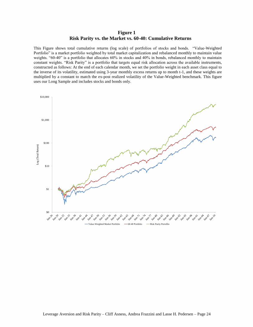
portfolios have done better than traditional portfolios. Figure 1 shows the growth of $1 since

1926 in a 60/40 portfolio, in a portfolio that weights by the ex-ante market cap of each asset

class, and, finally, in a simple version of a Risk Parity portfolio. While we show one case

here, the historical outperformance of Risk Parity is quite robust. In sum, the popular case

for Risk Parity investing rests on (1) the intuitive superiority of balancing risk and not dollars

invested and (2) the historical evidence for this approach over traditional approaches.

While these arguments are alluring, they are insufficient. Starting with (1) above, the

intuition that a risk balanced portfolio is always better relies on an implicit assumption about

expected returns. If the expected return of stocks were high enough versus bonds (a high

enough “equity risk premium”) you would gladly invest in a portfolio whose risk was equity

dominated. The intuition that 60/40 investors take too much risk in equities at all is only

accurate if the equity risk premium versus bonds is not high enough to support such a large

risk allocation. The more specific intuition of “equal risk” is only accurate in the specific

case of each asset possessing equal risk-adjusted returns.

In other words, you can’t just assert that equal risk is optimal because it is better

diversified. Rather, to believe that, you must believe you are not getting paid enough in

equities to be so concentrated in them. You cannot think of Risk Parity as only a statement

about divvying up risks, as it’s inherently also a statement about your views on expected

return. A Risk Parity investor should not say “equal risk is always the best regardless of

expected returns.” Instead, they should say “we do not believe expected returns are high

enough on equities to make them a disproportionate part of our risk budget.” That’s an

important distinction lost in the current discussion of Risk Parity. According to the CAPM,

the risk premia are exactly such that the market portfolio is optimal, so Risk Parity investors

need to explain how the CAPM fails in a way that justifies a larger allocation to low-risk

assets than their allocation in the market portfolio.

Let’s turn to (2), the empirical support that a Risk Parity portfolio has outperformed

over the long-term. It is indeed useful and relevant evidence in favor of Risk Parity, but it’s

also only one draw from history (admittedly a decently long one). We have to ask if this is

enough? Does the equity premium over bonds not being large enough over the last 80+ years


mean it won’t be large enough going forward? Ideally, we would like to have some out-of-

sample evidence, but waiting another 80 years seems an unappealing strategy. We propose

another route to potentially increase our confidence.

The missing links are i) a theoretical justification for Risk Parity investing, combined

with ii) broad tests across and within the major asset classes and countries. Frazzini and

Pedersen (2010) present these links. Following Fischer Black (1972), they show that if some

investors are averse to leverage, low-beta assets will offer higher risk-adjusted returns, and

high-beta assets lower risk-adjusted returns. Leverage aversion breaks the standard CAPM,

and according to this theory the highest risk-adjusted return is not achieved by the market,

but by a portfolio that over-weights safer assets. Thus, an investor who is less leverage averse

(or less leverage constrained) than the average investor can benefit by overweighting low-

beta assets, underweighting high-beta assets, and applying some leverage to the resulting

portfolio.

Empirically, Frazzini and Pedersen (2010) find consistent evidence of this theory within

each major asset class. They find that low-beta stocks have higher risk-adjusted returns than

high-beta stocks in the U.S. (echoing Black, Jensen, and Scholes (1972)) and in global stock

markets, safer corporate bonds have higher risk-adjusted returns than riskier ones, safer

short-maturity Treasuries offer higher risk-adjusted returns than riskier long-maturity ones,

and similarly within several other asset classes.3

As applied to Risk Parity, bonds are the low-beta asset, stocks the high-beta asset, and

the benefit of over-weighting bonds is another empirical success of the theory. We find that a

Risk Parity portfolio has realized higher risk-adjusted returns than the 60-40 portfolio in each

of the 11 countries covered by the JP Morgan Global Government Bond Index, providing

global out-of-sample evidence.

The theory of leverage aversion not only constitutes a theoretical underpinning for Risk

3 This evidence complements the large literature documenting that the CAPM is violated empirically (Fama and

French (1992), Gibbons (1982), Kandel (1984), Karceski (2002), Shanken (1985)). Given the strong

assumptions underlying the CAPM, it should perhaps not be a surprise that it is rejected empirically. Indeed, the

CAPM assumes that markets are without any frictions and that all investors can use any amount of leverage.

According to the CAPM, everyone holds the market portfolio (possibly levered) – which is clearly not the case

in the real world. However, that these violations tend to go the same way, higher returns on low beta assets

than forecast, is very interesting.


Parity, but it also highlights how further out-of-sample empirical evidence can be achieved

by comparing the risk-adjusted returns of safer vs. riskier securities within each of the major

asset classes. Leverage and margin constraints can also explain deviations from the Law of

One Price (Garleanu and Pedersen (2009)), the effects of central banks’ lending facilities

(Ashcraft, Garleanu, and Pedersen (2010)), and general liquidity dynamics (Brunnermeier

and Pedersen (2009)). Having the theory hold up in many other applications (without notable

exception) completely separate from the asset allocation decision studied here, makes us far

more confident that the empirical superiority of Risk Parity is not a statistical fluke, but

rather one more feather in the cap of Fisher Black’s theory, and one more instance to add to

the many in Frazzini and Pedersen (2010).4

The rest of the paper is organized as follows. First we lay out our theory of leverage

aversion. We present the investment opportunity set for investors who cannot use leverage.

As an alternative to leverage, these investors overweight riskier assets, and this increases the

equilibrium price of riskier assets or, said differently, reduces the expected return on riskier

assets. As a result, if some investors face such leverage constraints or margin requirements,

then the market portfolio is not the portfolio with the highest Sharpe ratio as the standard

CAPM predicts. Instead, the portfolio with the highest Sharpe ratio over-weights safer assets

and under-weights riskier assets, just like the RP portfolio. Next we test the theory's

implications for asset allocation. We find that the portfolio with the highest ex post Sharpe

indeed over-weights safer asset classes. Further, we find that the implementable RP portfolio

is close to the (unimplementable) ex post optimal portfolio. Finally we present the theory's

predictions for security selection within asset classes. We point out how the strong

consistent evidence that safer assets offer higher risk-adjusted returns than riskier ones

constitutes an important out-of-sample test that our story for risk-parity is not limited to the

4 Naturally, there are other hypotheses that produce higher risk-adjusted returns of safe assets versus riskier

assets. The alternatives include models of delegated portfolio management with benchmarked institutional

investors (Brennan (1993), Baker, Bradley, and Wurgler (2010)), mutual fund managers’ incentive to over-

weight high beta stocks due to the option-like payoffs generated by the convexity of the flow-performance

relation (Falkenstein (1994) and Karceski (2002)), or money illusion (Cohen, Polk, and Vuolteenaho (2005)).

Our result is also related to the low return to stocks with high idiosyncratic volatility (Ang, Hodrick, Xing,

Zhang (2006)) though that finding only applies to the recent volatility of illiquid securities (Li and Sullivan

(2011)) while the beta effect is more robust (Frazzini and Pedersen (2010)). Each of these alternatives delivers

predictions that apply to a specific setting (for example the universe of active equity mutual fund managers)

and, as a result, can explain some but not all of the evidence within and across each of the major asset classes.

They can of course be complementary to our unified leverage aversion theory.


successful history documented in Figure 1. Details about our data and portfolio construction

are in the Appendix.

A Theory of Leverage Aversion

Before we introduce leverage aversion, let us revisit the standard predictions of Modern

Portfolio Theory (MPT) of Markowitz (1952) and the Capital Asset Pricing Model (CAPM)

of Sharpe (1964), Lintner (1965) and Mossin (1966). MPT considers how an investor should

choose a portfolio with a good trade-off between risk and expected return. This is often

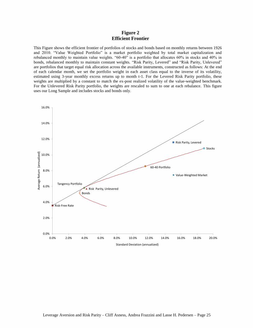
illustrated using a mean-volatility diagram as in Figure 2. We use data on realized returns for

U.S. stocks and Treasuries from 1926 to 2010 to estimate risk and expected returns. The

figure shows that the overall stock market has had average returns of 10.8% per year with a

volatility of 18.9%, while the overall bond market provided a lower average return of 5.2% at

a lower volatility of 3.4%. The hyperbola connecting these two points represents all possible

portfolios of stocks and bonds. For instance, the 60-40 portfolio represents an investment of

60% of capital in stocks and 40% of capital in bonds. (This portfolio is rebalanced every

month to these weights.)

The diagram also shows that the risk-free T-bill rate has averaged 3.6% per year,

represented by the point at the y-axis. Combining investments in the risk-free asset with

investments in risky assets produces lines connecting the risk-free point to the hyperbola.

The best such line for an investor who prefers higher returns and lower risk is the line from

the risk-free point to the so-called tangency portfolio, namely the portfolio with the highest

possible realized Sharpe ratio. In our data, the ex-post tangency portfolio invests 88% in

bonds and 12% in stocks. MPT says that an optimal portfolio is somewhere on this line:

Risk-averse investors’ portfolios should be between the tangency and the risk-free, investing

some money in cash and the rest in the tangency portfolio. Risk-tolerant investors should be

on the line segment extending beyond the tangency portfolio, meaning that they should use

leverage (i.e., borrowing at the risk-free rate rather than investing at the risk-free rate) to

invest more than 100% of their capital in the tangency portfolio.

The CAPM goes beyond MPT by assuming that all investors in fact invest in this way

and concludes as a result that the tangency portfolio must be equal to the market portfolio,


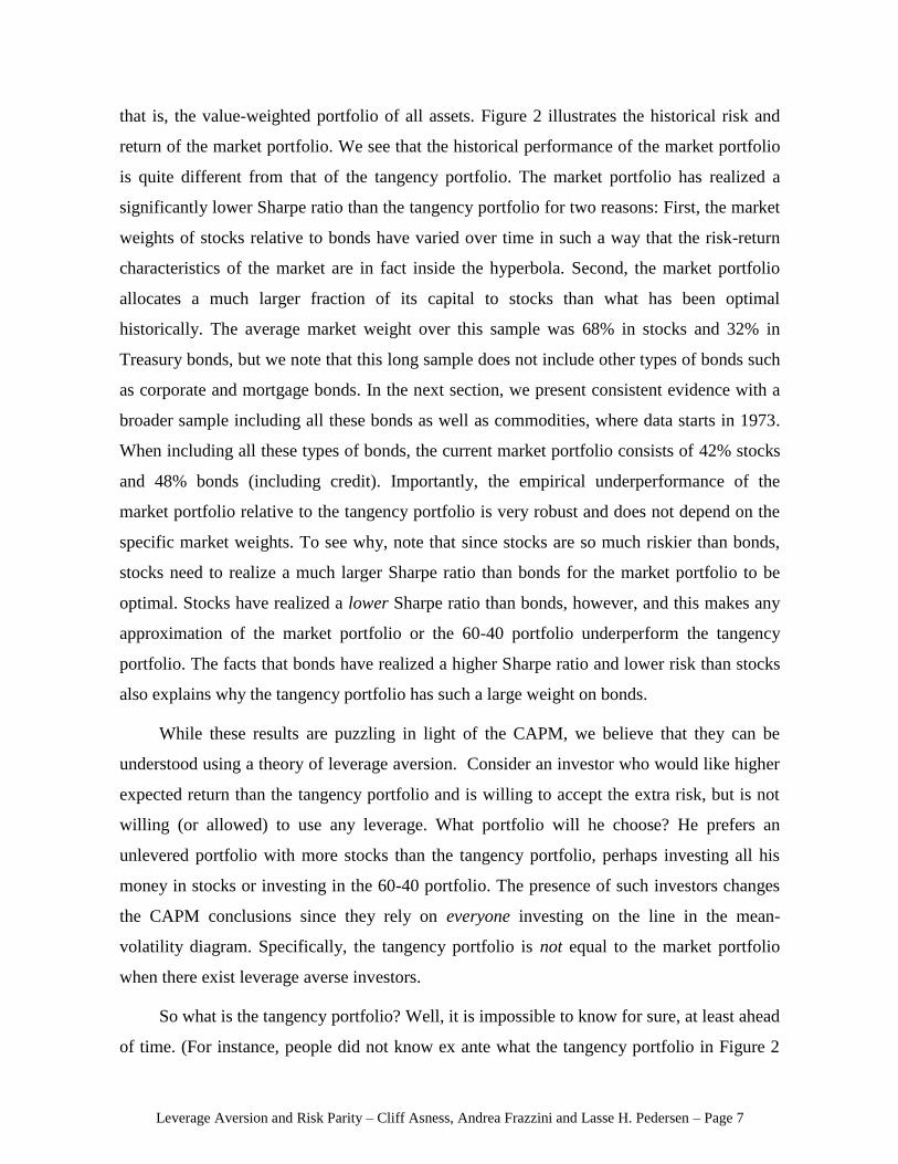
that is, the value-weighted portfolio of all assets. Figure 2 illustrates the historical risk and

return of the market portfolio. We see that the historical performance of the market portfolio

is quite different from that of the tangency portfolio. The market portfolio has realized a

significantly lower Sharpe ratio than the tangency portfolio for two reasons: First, the market

weights of stocks relative to bonds have varied over time in such a way that the risk-return

characteristics of the market are in fact inside the hyperbola. Second, the market portfolio

allocates a much larger fraction of its capital to stocks than what has been optimal

historically. The average market weight over this sample was 68% in stocks and 32% in

Treasury bonds, but we note that this long sample does not include other types of bonds such

as corporate and mortgage bonds. In the next section, we present consistent evidence with a

broader sample including all these bonds as well as commodities, where data starts in 1973.

When including all these types of bonds, the current market portfolio consists of 42% stocks

and 48% bonds (including credit). Importantly, the empirical underperformance of the

market portfolio relative to the tangency portfolio is very robust and does not depend on the

specific market weights. To see why, note that since stocks are so much riskier than bonds,

stocks need to realize a much larger Sharpe ratio than bonds for the market portfolio to be

optimal. Stocks have realized a lower Sharpe ratio than bonds, however, and this makes any

approximation of the market portfolio or the 60-40 portfolio underperform the tangency

portfolio. The facts that bonds have realized a higher Sharpe ratio and lower risk than stocks

also explains why the tangency portfolio has such a large weight on bonds.

While these results are puzzling in light of the CAPM, we believe that they can be

understood using a theory of leverage aversion. Consider an investor who would like higher

expected return than the tangency portfolio and is willing to accept the extra risk, but is not

willing (or allowed) to use any leverage. What portfolio will he choose? He prefers an

unlevered portfolio with more stocks than the tangency portfolio, perhaps investing all his

money in stocks or investing in the 60-40 portfolio. The presence of such investors changes

the CAPM conclusions since they rely on everyone investing on the line in the mean-

volatility diagram. Specifically, the tangency portfolio is not equal to the market portfolio

when there exist leverage averse investors.

So what is the tangency portfolio? Well, it is impossible to know for sure, at least ahead

of time. (For instance, people did not know ex ante what the tangency portfolio in Figure 2


would turn out to be.) However, a theory of equilibrium with leverage aversion provides

some guidance. Frazzini and Pedersen (2010) show that the tangency portfolio over-weights

safer assets, just as is the case empirically. This result is intuitive: Since some investors

choose to overweight riskier assets to avoid leverage, the price of riskier assets is elevated or,

equivalently, the expected return on riskier assets is reduced. In contrast, the safer assets are

under-weighted by these investors, and therefore trade at low prices, i.e., offer high expected

returns. Hence, investors who are able and willing to apply leverage can achieve higher risk-

adjusted returns by having the opposite portfolio tilts, namely over-weighting safer assets. In

other words, leverage risk is rewarded in equilibrium through the relative pricing of

securities. This is why the tangency portfolio consists of a disproportional amount of safer

assets.

The specific composition of the tangency portfolio depends on how many leverage

constrained investors there are and this can change over time. Hence, in practice, we cannot

know for sure what is the tangency portfolio. However, Risk Parity (RP) investing offers a

simple suggestion, which is in the direction suggested by the leverage aversion theory: RP

investments allocate the same amount of risk to stocks and bonds.

Specifically, we construct a simple RP portfolio as follows: At the end of each calendar

month, we set the portfolio weight in each asset class equal to the inverse of its volatility,

estimated using 3-year monthly excess returns up to month t-1, and these weights are

multiplied by a constant to match the ex-post realized volatility of the value-weighted

benchmark. We note that this simple construction does not rely on covariance estimates.

Over the full sample this means investing on average 15% in stocks and 85% in bonds on an

unlevered basis. The most recent Risk Parity allocations (as of June 2010) are 86% in bonds

and 14% in stocks.

Figure 2 shows that the historical performance of the RP portfolio is more similar to

that of the tangency portfolio than either the market or the 60-40 portfolios. As seen in the

Figure 2, despite being not exactly ex post optimal, the RP portfolio has been a good

approximation since over-weighting safer assets has paid off. While we should not take the

precise prescription to have exactly equal risk in stocks and bonds (parity) too seriously, it is

quite a strong and accurate move in the right direction ex post.


The leverage aversion theory is laid out more formally by Frazzini and Pedersen

(2010), who also present several other testable asset pricing predictions. Further, according to

this theory, no one holds the market portfolio, but equilibrium is achieved nevertheless since

some investors over-weight safer assets while others over-weight riskier assets. Both groups

of investors are satisfied: Some accept low Sharpe ratios but achieve high expected returns

without leverage; others achieve high expected returns with a better risk-return tradeoff by

using leverage.

Risk and Return Across Asset Classes: Risk Parity vs. the Market vs. 60-40

To test our predicted implications of leverage aversion, we compare the historical

performance of the value-weighted market portfolio, the Risk Parity portfolio, and the 60-40

stock/bond portfolio. We do this over three different data samples: Our “Long Sample”

covers U.S. stocks and bonds from 1926 to 2010; our “Broad Sample” covers global stocks,

U.S. bonds, credit, and commodities from 1973 to 2010; and our “Global Sample” covers

stocks and bonds in the 11 countries covered by the JP Morgan Global Government Bond

Index from 1986 to 2010. Summary statistics are seen in Table 1 and further details on the

data and the portfolios are in the appendix.

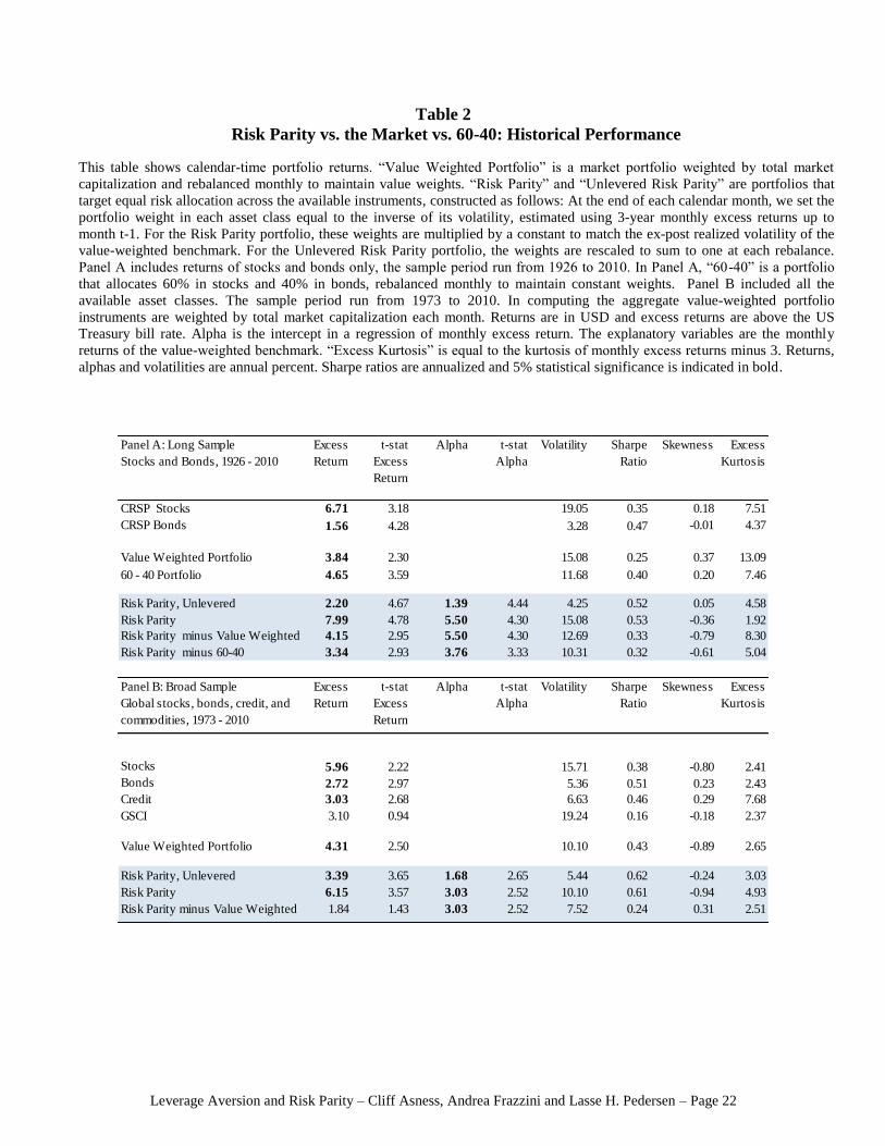
Table 2 shows the performance statistics, with Panel A using our Long Sample, while

Panel B covers the Broad Sample. In both cases, we see that stocks have delivered higher

average returns than bonds, and stocks have realized much higher volatility than bonds. As a

result, the value-weighted market portfolio and the 60-40 portfolio have had higher average

returns than the unlevered Risk Parity portfolio. Therefore, an investor who cannot and/or

will not use leverage may prefer to hold the market or the 60-40 portfolio or even all stocks,

and such behavior is what can cause riskier assets to be overpriced relative to the standard

CAPM.

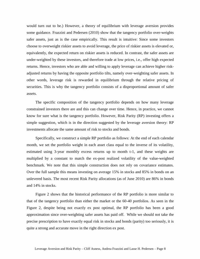
An investor who is able to use leverage will prefer the historical performance of the

Risk Parity portfolio, however, because of its higher Sharpe ratio (risk-adjusted return).

Indeed, the levered Risk Parity portfolio has the same volatility as the market portfolio, but a

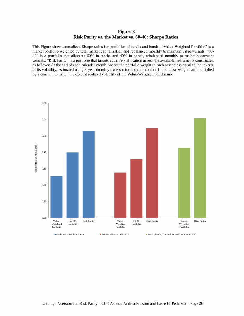
considerably higher average return. Figure 3 illustrates the significant improvement in

Sharpe ratio of the Risk Parity portfolio over the market and 60-40 portfolios.


We note that our simulated performance of the levered RP portfolio does not attempt to

adjust the returns for the cost of leverage such as financing spreads and costs associated with

de-levering. When leverage is applied using futures, there is no financing spread and our

results are similar with futures returns. At modest levels of leverage, any additional costs of

leverage should also be quite low, while at high levels of leverage, the potential cost of

forced de-levering could be much more meaningful, especially for an investor with a large

overall portfolio. Appendix B shows the robustness of the results with respect to different

financing rates.

The strong historical performance of Risk Parity is also seen in the cumulative return

plot illustrated in Figure 1 (as discussed in the introduction). To test the significance of this

outperformance, Table 2 reports the t-statistic of the Risk Parity portfolio’s realized alpha.

Here, alpha is the intercept in a time series regression of monthly excess return on the value-

weighted benchmark. The t-statistics are far north of 2 implying strong statistical

significance. As a further test, we construct long-short portfolios that go long the Risk Parity

portfolio and go short the market portfolio (or go short the 60-40 portfolio) over each sample.

These long-short portfolios have statistically significant excess returns and alphas over both

our Long Sample and our Broad Sample.

You might worry that the superiority of Risk Parity is an artifact of the bond bull

market over the last 25-30 years. But, looking at this longer 1926-present period we see a

near perfect round trip in bond yields, and a near doubling of the equity market's valuation

(using the 10-year P/Es of Robert Shiller5), so if anything 1926-present is a period biased to

favor equities over bonds, yet we still find that risk-parity has been a superior strategy.

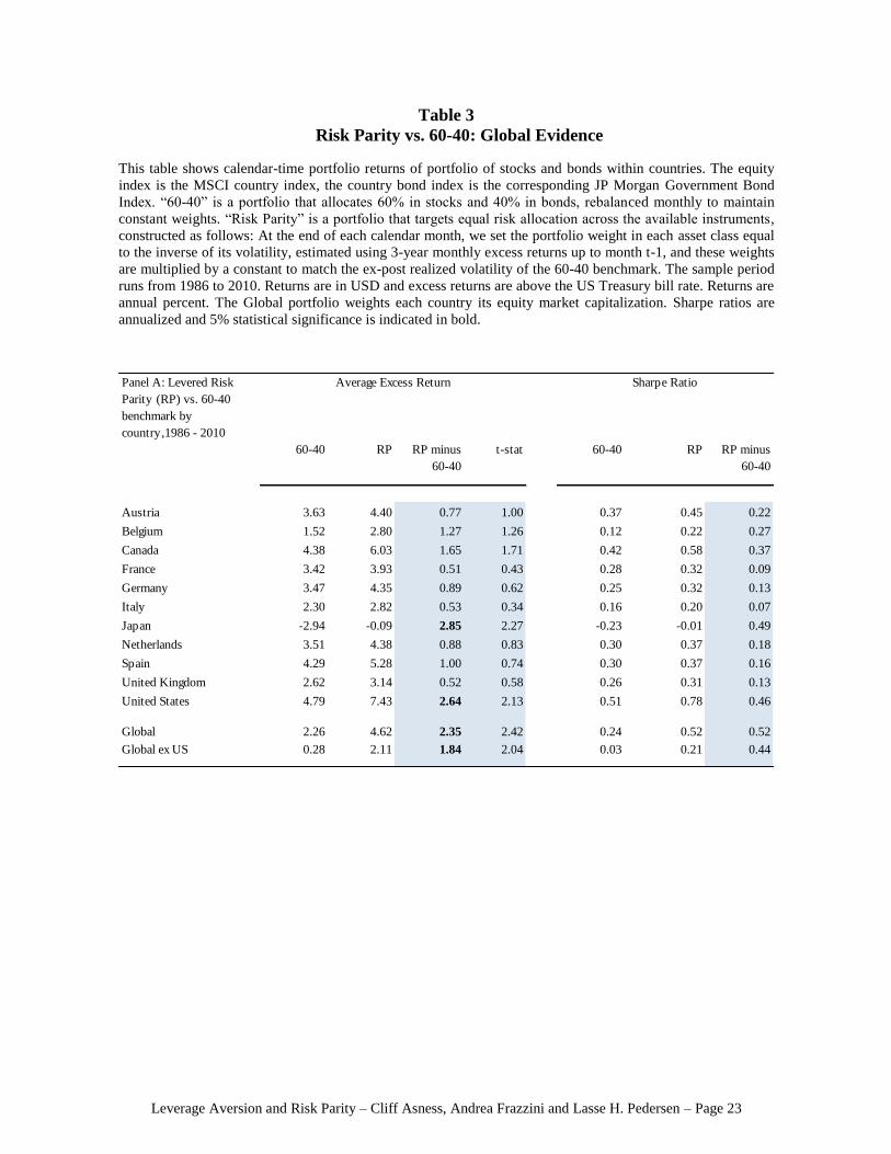
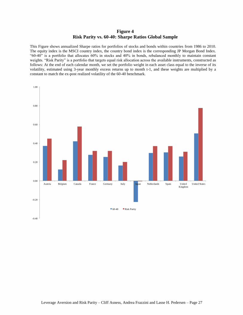
To complement the evidence from our long and broad U.S. samples, Table 3 provides

global evidence from 10 other countries. For each country, we find that the Risk Parity

portfolio has provided higher risk-adjusted returns than the 60-40 portfolio. The

outperformance on the RP portfolio is statistically significant when pooling all countries into

a (value-weighted) global portfolio with and without the US. Figure 4 shows the relative

performance of RP over 60-40 in each country.

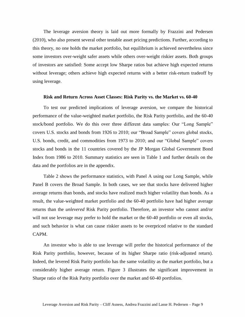
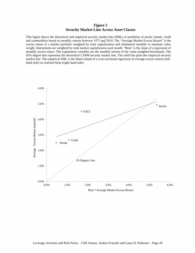
A classic illustration of the empirical failure of the standard CAPM is the notion that

5 Data can be downloaded at http://www.econ.yale.edu/~shiller/data.htm

http://www.econ.yale.edu/~shiller/data.htm


the “Security Market Line is too flat,” originally pointed out by Black, Jensen, and Scholes

(1972) for U.S. stocks. The Security Market Line is the connection between the actual excess

return across securities and the CAPM-predicted excess returns, given by beta times the

market excess return. Rather than looking at the Security Market Line across stocks, we are

interested in the Security Market Line across assets classes. Figure 5 shows the Security

Market Line for the asset classes in our Broad Sample, where betas are the slopes from a

time series regression of monthly excess return on the value-weighted benchmark.

The CAPM predicts that securities line up on the 45 degree line, meaning that securities

expected return line up with their systematic risk. However, Figure 5 shows that the

empirical Security Market Line is more flat since safer asset classes (bonds, credit, GSCI)

provide too high returns relative to the CAPM, while riskier asset classes (domestic and

global stocks) provide too low returns relative to their risk. We note that while commodities

(as captured by the GSCI index) have high volatility, their systematic beta risk is in fact

significantly below that of the stock market due to commodities’ low correlation to the

market. This flatness of the Security Market Line underlies the power of buying safer assets,

and the security market line is also flat in other countries and through our long sample

(Figures 1 and 4).


Risk and Return within Asset Classes: High Beta is Low Alpha

Our evidence that the Security Market Line is too flat holds not just across asset

classes, but also within asset classes. Said differently, safer assets have higher risk-adjusted

returns than riskier assets when comparing securities within the same asset class, just as in

the case of comparing across asset classes.

Indeed, Black, Jensen and Scholes (1972) famously found that the Security Market

Line is too flat across U.S. stocks. Frazzini and Pedersen (2010) confirm this finding adding

40 years of out-of-sample evidence: the Security Market Line has remained remarkably flat

since the study of Black, Jensen and Scholes. Further, Frazzini and Pedersen (2010) find that

the Security Market Line is also too flat in all the other major asset classes. It is too flat in

global stocks markets, in 18 of 19 developed equity markets, across Treasuries, across

corporate bonds, and even across futures.

The within-asset-class results are important to the inherently across-asset-class results

of risk-parity, as they represent strong out-of-sample confirmation that what’s going on for

asset classes is ubiquitous and thus less likely an artifact of data mining.

Conclusion: You Can Eat Risk Adjusted Returns

Risk Parity investing has become a popular alternative to traditional methods of

strategic asset allocation. However, existing justifications are insufficient and fail to provide

a consistent equilibrium theory. It is not enough to simply desire diversification by risk not

dollars, however intuitive. If you were paid enough in expected return to be dominated in

risk-space by a single asset class you'd do so gladly. It's not enough to show that historically

you have not in fact been paid enough to be so dominated (the equivalent of a backtest

showing that Risk Parity is historically superior to traditional allocations). Historical

evidence is always welcome, but even long histories of asset class return can be dominated

by a few large data points or arise from data mining. Risk Parity investors need not despair,

however. While there is no certainty in finance, perhaps the closest we ever come is a

realistic theory that holds up consistently in out-of-sample tests across and within different

asset classes and countries. Leverage aversion, pioneered by Black (1972, 1992) is such a

theory.


Assuming that some market participants are unable or unwilling to use leverage is not

unrealistic. Leverage simply presents a risk that investors want to be compensated for

bearing. Further, to obtain and manage leverage requires acquiring a certain “technology”.

Indeed, obtaining leverage requires getting financing, using derivatives, and establishing

counterparty relations. Managing the leverage requires adjusting margin accounts, and

dynamic trading the portfolio over time, among other things. Our capital markets present

plenty of examples of investors that are not allowed (or choose not) to employ leverage to

increase their returns. For example, the majority of mutual funds and many pension funds are

prevented from borrowing or limited in the amount of leverage they can take. As another

example, mutual fund families typically provide suggested asset allocations for low to high

risk tolerant investors. The high risk recommendations rarely use leverage, but rather

recommend a very extreme concentration in equities. Similarly, the rise of embedded

leverage in exchange traded funds (ETFs) shows that some investors choose not to employ

leverage directly, but prefer instruments with embedded leverage.

To put the magnitude of investors’ model-implied leverage aversion in perspective, we

can estimate the opportunity of investing in the value-weighted market portfolio instead of

Risk Parity portfolio. Over 1926-2010, Risk Parity has realized a Sharpe Ratio that is 0.27

higher than the market portfolio, meaning that an investor with an average volatility of 10%

invested in the value-weighted market portfolio has underperformed the Risk Parity portfolio

by 2.7% per year. For investors with high costs of and aversion to leverage, this number may

not make them switch to Risk Parity, while other investors can benefit from using leverage.

The results in Black, Jensen, and Scholes (1972) and Frazzini and Pedersen (2010)

show that the predictions of a theory of leverage aversion hold up in a very wide variety of

tests across and within many asset classes. This paper shows that Risk Parity investing is

simply another instance of this theory working out of sample, and thus greatly enhances our

confidence that Risk Parity's superiority to traditional methods is not a figment of the data

but real and important.


References

Ang, A., R. Hodrick, Y. Xing, X. Zhang (2006), “The Cross-Section of Volatility and

Expected Returns,” Journal of Finance, 61, pp. 259-299.

Ashcraft, A., N. Garleanu, and L.H. Pedersen (2010), “Two Monetary Tools: Interest Rates

and Haircuts,” NBER Macroeconomics Annual, forthcoming.

Asness, C.S. (1996), “Why Not 100% Equities,” The Journal of Portfolio Management, Vol.

22:2, 29-34.

Asness, C.S. (Sept/Oct 2010), “Speculative Leverage: A False Cure for Pension Woes A

Comment”, Financial Analysts Journal, Volume 66 Number 5, 14-15.

Baker, M., B. Bradley, and J. Wurgler (2010), “Benchmarks as Limits to Arbitrage:

Understanding the Low Volatility Anomaly,” working paper, Harvard.

Black, F. (1972), “Capital market equilibrium with restricted borrowing,” Journal of

business, 45, 3, pp. 444-455.

– (1992), “Beta and Return,” The Journal of Portfolio Management, 20, pp. 8-18.

Black, F., M.C. Jensen, and M. Scholes (1972), “The Capital Asset Pricing Model: Some

Empirical Tests.” In Michael C. Jensen (ed.), Studies in the Theory of Capital Markets, New

York, pp. 79-121.

Brennan, M.J. (1993), “Agency and Asset Pricing.” University of California, Los Angeles,

working paper.

Brunnermeier, M. and L.H. Pedersen (2009), “Market Liquidity and Funding Liquidity,” The

Review of Financial Studies, 22, 2201-2238.


Cohen, R.B., C. Polk, and T. Vuolteenaho (2005), “Money Illusion in the Stock Market: The

Modigliani-Cohn Hypothesis,” The Quarterly Journal of Economics, 120:2, 639-668.

Falkenstein, E.G. (1994), “Mutual funds, idiosyncratic variance, and asset returns”,

Dissertation, Northwestern University.

Fama, E.F. and French, K.R. (1992), “The cross-section of expected stock returns,” Journal

of Finance, 47, 2, pp. 427-465.

Frazzini, A. and L. H. Pedersen (2010), “Betting Against Beta”, working paper, AQR Capital

Management, New York University and NBER (WP 16601).

Garleanu, N., and L. H. Pedersen (2009), “Margin-Based Asset Pricing and Deviations from

the Law of One Price," UC Berkeley and NYU, working paper.

Gibbons, M. (1982), “Multivariate tests of financial models: A new approach,” Journal of

Financial Economics, 10, 3-27.

Kandel, S. (1984), “The likelihood ratio test statistic of mean-variance efficiency without a

riskless asset,” Journal of Financial Economics, 13, pp. 575-592.

Karceski, J. (2002), “Returns-Chasing Behavior, Mutual Funds, and Beta’s Death,” Journal

of Financial and Quantitative Analysis, 37:4, 559-594.

Li, Xi and Rodney N. Sullivan (2010), “The Limits to Arbitrage Revisited: The Low-Risk

Anomaly,” Boston College, working paper.

Lintner, J. (1965), “The valuation of risk assets and the selection of risky investments in

stock portfolios and capital budgets”, Review of Economics and Statistics, 47, 13-37.

Markowitz, H.M. (1952), “Portfolio Selection,” The Journal of Finance, 7, 77-91.


Mossin, J. (1966), “Equilibrium in a Capital Asset Market”, Econometrica, 34, 768–783.

Shanken, J. (1985), “Multivariate tests of the zero-beta CAPM,” Journal of Financial

Economics, 14,. 327-348.

Sharpe, W. F. (1964), “Capital asset prices: A theory of market equilibrium under conditions

of risk”, Journal of Finance, 19, 425-442.

Sullivan, Rodney (May/June 2010), “Speculative Leverage: A False Cure for Pension

Woes”, Financial Analysts Journal, Volume 66 Number 3, 6-8.


Appendix A: Data and Portfolio Construction

We test our theory in several complementary ways. We use three samples: Our Long

Sample from January 1926 to June 2010 consists of U.S. stocks and government bonds; our

Broad Sample from January 1973 to June 2010 consists of global stocks, bonds, corporate

bonds, and commodities; and our Global Sample consists of stocks and bonds for all

countries belonging to the JP Morgan Global Government Bond Index.

The return and market capitalization data for the Long Sample is drawn from the CRSP

database. We use the CRSP value-weighted market return (including dividends) as the

aggregate stock return. Similarly, our aggregate bond return is the value-weighted average of

the unadjusted holding period return for each bond in the CRSP Monthly US Treasury

Database. Bonds are weighted by their outstanding face value.

To include data on various types of government bonds, credit-risky bonds, and

commodities in our Broad Sample, we need to restrict attention to the more recent time

period from January 1973 to June 2010. In our Broad Sample, bonds are the sum of the

Treasury and Other Government Bond series from Barclays Capital’s Bond Hub database.6

For credit, we use the sum of all credit-related and securitized series in Barclays Universal

index, as detailed in Table 1. Finally, we use the S&P GSCI index as a benchmark for

investment in commodity markets obtained from Bloomberg.7 As a proxy for commodities’

total market capitalization we use the annual total dollar value of commodity production,

provided to us by Merrill Lynch8. Since our commodity production data starts in 1989, we

use the 1989 weight between 1973 and 1988.9 All returns and market capitalization series are

in USD and excess returns are above the US Treasury bill rate.

Our Global sample consists of stocks and bonds. Our global stock market proxy is the

MSCI World indices provided by MSCI/Barra.10

For bonds, we use the JP Morgan Global

Government Bond indices from Datastream. The sample runs from January 1986 to June

2010.

6 The data can be downloaded at https://live.barcap.com

7 Formerly the Goldman Sachs Commodity Index

8 We would like to thank Merrill Lynch Commodities Inc. for making this data available to us

9 Our results are robust to dropping commodities from 1973 to 1988 where we do not have total dollar

production data. 10

The data can be downloaded at: http://www.mscibarra.com

https://live.barcap.com/

http://www.mscibarra.com/


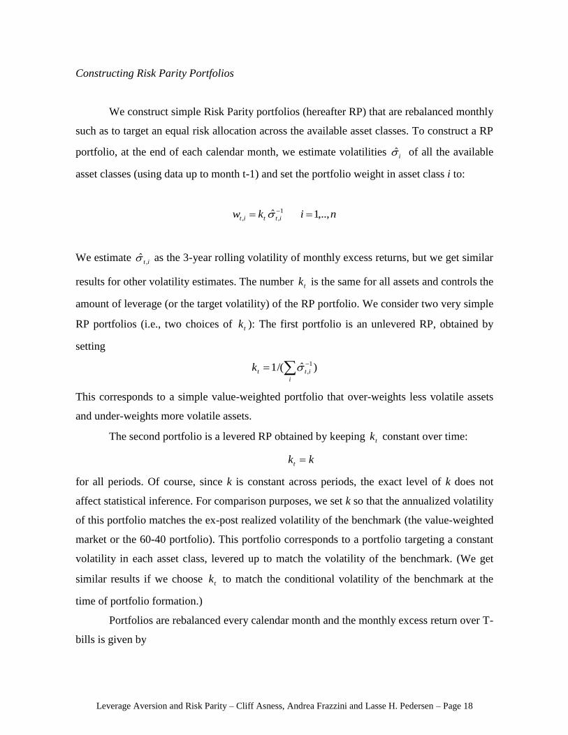
Constructing Risk Parity Portfolios

We construct simple Risk Parity portfolios (hereafter RP) that are rebalanced monthly

such as to target an equal risk allocation across the available asset classes. To construct a RP

portfolio, at the end of each calendar month, we estimate volatilities i of all the available

asset classes (using data up to month t-1) and set the portfolio weight in asset class i to:

nikw ittit ,..,1ˆ 1

,,

We estimate it , as the 3-year rolling volatility of monthly excess returns, but we get similar

results for other volatility estimates. The number tk is the same for all assets and controls the

amount of leverage (or the target volatility) of the RP portfolio. We consider two very simple

RP portfolios (i.e., two choices of tk ): The first portfolio is an unlevered RP, obtained by

setting

)ˆ/(1 1

, i

ittk

This corresponds to a simple value-weighted portfolio that over-weights less volatile assets

and under-weights more volatile assets.

The second portfolio is a levered RP obtained by keeping tk constant over time:

kkt

for all periods. Of course, since k is constant across periods, the exact level of k does not

affect statistical inference. For comparison purposes, we set k so that the annualized volatility

of this portfolio matches the ex-post realized volatility of the benchmark (the value-weighted

market or the 60-40 portfolio). This portfolio corresponds to a portfolio targeting a constant

volatility in each asset class, levered up to match the volatility of the benchmark. (We get

similar results if we choose tk to match the conditional volatility of the benchmark at the

time of portfolio formation.)

Portfolios are rebalanced every calendar month and the monthly excess return over T-

bills is given by


)( ,,1 tit

i

it

RP

t rfrwr

where r is the month-t USD gross return and rf is the 1-month Treasury bill rate. Table 1

reports the list of instruments.


Appendix B: Robustness and Financing Costs

Our results on risk parity investment are robust. We have presented the performance

using both a Long, a Broad, and a Global data set, and we have checked that our main

conclusions robust to slight modifications to our portfolio construction methodology (not

reported).

As a further robustness check, this appendix studies the performance if we change

which interest rate is used as the risk-free rate. Whereas the main analysis follows the

literature by using the Treasury-Bill rate, Table B.1 also considers the repo, OIS, Fed Funds,

and LIBOR rates. Given that the RP portfolio is levered, its performance is reduced when the

risk-free rate is higher. Nevertheless, the RP portfolio outperforms the market portfolio even

with the most conservative LIBOR interest rate as seen in the table. We note that leverage

can be achieved using futures contracts at an implicit cost that is lower than the LIBOR rate.

Financing costs and the ability to manage leverage over time may differ across

investors. Indeed, some investors may display greater leverage “aversion” because they face

greater financing costs and/or lower ability to manage the leverage over time.


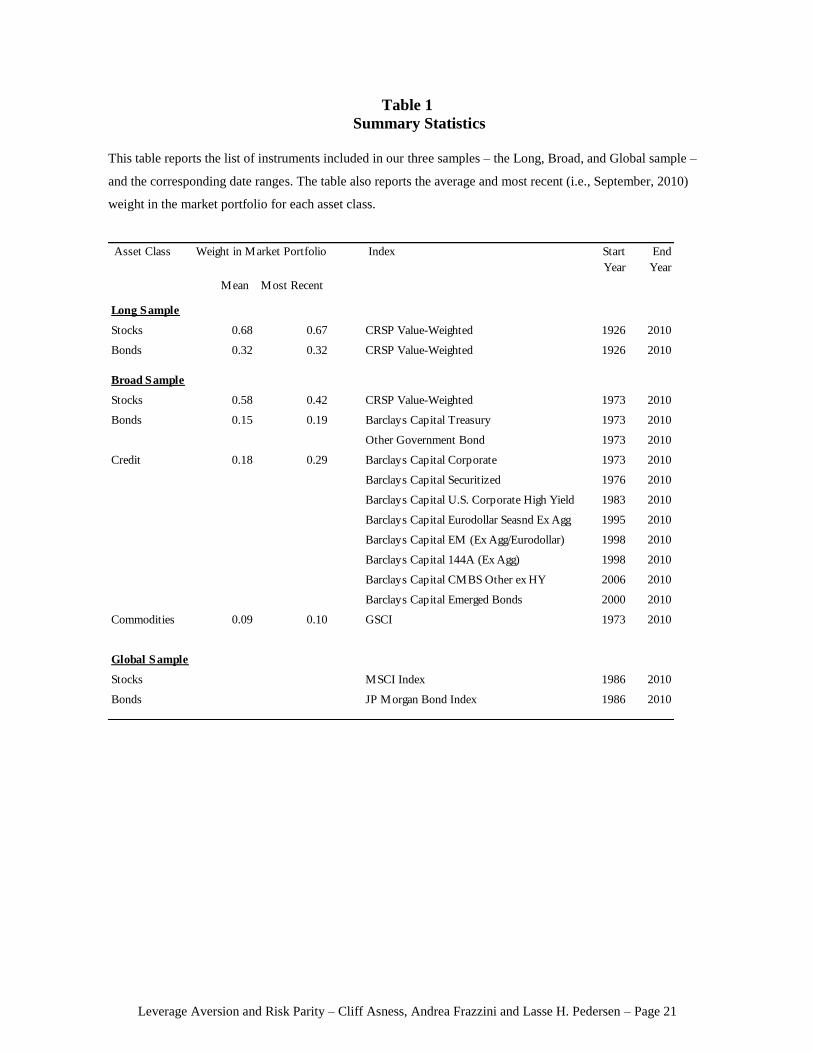
Table 1

Summary Statistics

This table reports the list of instruments included in our three samples – the Long, Broad, and Global sample –

and the corresponding date ranges. The table also reports the average and most recent (i.e., September, 2010)

weight in the market portfolio for each asset class.

Asset Class Index Start

Year

End

Year

Mean Most Recent

Long Sample

Stocks 0.68 0.67 CRSP Value-Weighted 1926 2010

Bonds 0.32 0.32 CRSP Value-Weighted 1926 2010

Broad Sample

Stocks 0.58 0.42 CRSP Value-Weighted 1973 2010

Bonds 0.15 0.19 Barclays Capital Treasury 1973 2010

Other Government Bond 1973 2010

Credit 0.18 0.29 Barclays Capital Corporate 1973 2010

Barclays Capital Securitized 1976 2010

Barclays Capital U.S. Corporate High Yield 1983 2010

Barclays Capital Eurodollar Seasnd Ex Agg 1995 2010

Barclays Capital EM (Ex Agg/Eurodollar) 1998 2010

Barclays Capital 144A (Ex Agg) 1998 2010

Barclays Capital CMBS Other ex HY 2006 2010

Barclays Capital Emerged Bonds 2000 2010

Commodities 0.09 0.10 GSCI 1973 2010

Global Sample

Stocks MSCI Index 1986 2010

Bonds JP Morgan Bond Index 1986 2010

Weight in Market Portfolio


Table 2

Risk Parity vs. the Market vs. 60-40: Historical Performance

This table shows calendar-time portfolio returns. “Value Weighted Portfolio” is a market portfolio weighted by total market

capitalization and rebalanced monthly to maintain value weights. “Risk Parity” and “Unlevered Risk Parity” are portfolios that

target equal risk allocation across the available instruments, constructed as follows: At the end of each calendar month, we set the

portfolio weight in each asset class equal to the inverse of its volatility, estimated using 3-year monthly excess returns up to

month t-1. For the Risk Parity portfolio, these weights are multiplied by a constant to match the ex-post realized volatility of the

value-weighted benchmark. For the Unlevered Risk Parity portfolio, the weights are rescaled to sum to one at each rebalance.

Panel A includes returns of stocks and bonds only, the sample period run from 1926 to 2010. In Panel A, “60-40” is a portfolio

that allocates 60% in stocks and 40% in bonds, rebalanced monthly to maintain constant weights. Panel B included all the

available asset classes. The sample period run from 1973 to 2010. In computing the aggregate value-weighted portfolio

instruments are weighted by total market capitalization each month. Returns are in USD and excess returns are above the US

Treasury bill rate. Alpha is the intercept in a regression of monthly excess return. The explanatory variables are the monthly

returns of the value-weighted benchmark. “Excess Kurtosis” is equal to the kurtosis of monthly excess returns minus 3. Returns,

alphas and volatilities are annual percent. Sharpe ratios are annualized and 5% statistical significance is indicated in bold.

Panel A: Long Sample

Stocks and Bonds, 1926 - 2010

Excess

Return

t-stat

Excess

Return

Alpha t-stat

Alpha

Volatility Sharpe

Ratio

Skewness Excess

Kurtosis

CRSP Stocks 6.71 3.18 19.05 0.35 0.18 7.51

CRSP Bonds 1.56 4.28 3.28 0.47 -0.01 4.37

Value Weighted Portfolio 3.84 2.30 15.08 0.25 0.37 13.09

60 - 40 Portfolio 4.65 3.59 11.68 0.40 0.20 7.46

Risk Parity, Unlevered 2.20 4.67 1.39 4.44 4.25 0.52 0.05 4.58

Risk Parity 7.99 4.78 5.50 4.30 15.08 0.53 -0.36 1.92

Risk Parity minus Value Weighted 4.15 2.95 5.50 4.30 12.69 0.33 -0.79 8.30

Risk Parity minus 60-40 3.34 2.93 3.76 3.33 10.31 0.32 -0.61 5.04

Panel B: Broad Sample

Global stocks, bonds, credit, and

commodities, 1973 - 2010

Excess

Return

t-stat

Excess

Return

Alpha t-stat

Alpha

Volatility Sharpe

Ratio

Skewness Excess

Kurtosis

Stocks 5.96 2.22 15.71 0.38 -0.80 2.41

Bonds 2.72 2.97 5.36 0.51 0.23 2.43

Credit 3.03 2.68 6.63 0.46 0.29 7.68

GSCI 3.10 0.94 19.24 0.16 -0.18 2.37

Value Weighted Portfolio 4.31 2.50 10.10 0.43 -0.89 2.65

Risk Parity, Unlevered 3.39 3.65 1.68 2.65 5.44 0.62 -0.24 3.03

Risk Parity 6.15 3.57 3.03 2.52 10.10 0.61 -0.94 4.93

Risk Parity minus Value Weighted 1.84 1.43 3.03 2.52 7.52 0.24 0.31 2.51


Table 3

Risk Parity vs. 60-40: Global Evidence

This table shows calendar-time portfolio returns of portfolio of stocks and bonds within countries. The equity

index is the MSCI country index, the country bond index is the corresponding JP Morgan Government Bond

Index. “60-40” is a portfolio that allocates 60% in stocks and 40% in bonds, rebalanced monthly to maintain

constant weights. “Risk Parity” is a portfolio that targets equal risk allocation across the available instruments,

constructed as follows: At the end of each calendar month, we set the portfolio weight in each asset class equal

to the inverse of its volatility, estimated using 3-year monthly excess returns up to month t-1, and these weights

are multiplied by a constant to match the ex-post realized volatility of the 60-40 benchmark. The sample period

runs from 1986 to 2010. Returns are in USD and excess returns are above the US Treasury bill rate. Returns are

annual percent. The Global portfolio weights each country its equity market capitalization. Sharpe ratios are

annualized and 5% statistical significance is indicated in bold.

Panel A: Levered Risk

Parity (RP) vs. 60-40

benchmark by

country,1986 - 2010

60-40 RP RP minus

60-40

t-stat 60-40 RP RP minus

60-40

Austria 3.63 4.40 0.77 1.00 0.37 0.45 0.22

Belgium 1.52 2.80 1.27 1.26 0.12 0.22 0.27

Canada 4.38 6.03 1.65 1.71 0.42 0.58 0.37

France 3.42 3.93 0.51 0.43 0.28 0.32 0.09

Germany 3.47 4.35 0.89 0.62 0.25 0.32 0.13

Italy 2.30 2.82 0.53 0.34 0.16 0.20 0.07

Japan -2.94 -0.09 2.85 2.27 -0.23 -0.01 0.49

Netherlands 3.51 4.38 0.88 0.83 0.30 0.37 0.18

Spain 4.29 5.28 1.00 0.74 0.30 0.37 0.16

United Kingdom 2.62 3.14 0.52 0.58 0.26 0.31 0.13

United States 4.79 7.43 2.64 2.13 0.51 0.78 0.46

Global 2.26 4.62 2.35 2.42 0.24 0.52 0.52

Global ex US 0.28 2.11 1.84 2.04 0.03 0.21 0.44

Average Excess Return Sharpe Ratio


Figure 1

Risk Parity vs. the Market vs. 60-40: Cumulative Returns

This Figure shows total cumulative returns (log scale) of portfolios of stocks and bonds. “Value-Weighted

Portfolio” is a market portfolio weighted by total market capitalization and rebalanced monthly to maintain value

weights. “60-40” is a portfolio that allocates 60% in stocks and 40% in bonds, rebalanced monthly to maintain

constant weights. “Risk Parity” is a portfolio that targets equal risk allocation across the available instruments,

constructed as follows: At the end of each calendar month, we set the portfolio weight in each asset class equal to

the inverse of its volatility, estimated using 3-year monthly excess returns up to month t-1, and these weights are

multiplied by a constant to match the ex-post realized volatility of the Value-Weighted benchmark. This figure

uses our Long Sample and includes stocks and bonds only.

$0

$1

$10

$100

$1,000

$10,000

Lo

g (

To

tal

Ret

urn

)

Value-Weighted Market Portfolio 60-40 Portfolio Risk Parity Portoflio


Figure 2

Efficient Frontier

This Figure shows the efficient frontier of portfolios of stocks and bonds based on monthly returns between 1926

and 2010. “Value Weighted Portfolio” is a market portfolio weighted by total market capitalization and

rebalanced monthly to maintain value weights. “60-40” is a portfolio that allocates 60% in stocks and 40% in

bonds, rebalanced monthly to maintain constant weights. “Risk Parity, Levered” and “Risk Parity, Unlevered”

are portfolios that target equal risk allocation across the available instruments, constructed as follows: At the end

of each calendar month, we set the portfolio weight in each asset class equal to the inverse of its volatility,

estimated using 3-year monthly excess returns up to month t-1. For the Levered Risk Parity portfolio, these

weights are multiplied by a constant to match the ex-post realized volatility of the value-weighted benchmark.

For the Unlevered Risk Parity portfolio, the weights are rescaled to sum to one at each rebalance. This figure

uses our Long Sample and includes stocks and bonds only.

Risk-Free Rate

Tangency Portfolio

Value-Weighted Market

60-40 Portfolio

Risk Parity, Levered

Risk Parity, Unlevered

Stocks

Bonds

0.0%

2.0%

4.0%

6.0%

8.0%

10.0%

12.0%

14.0%

16.0%

0.0% 2.0% 4.0% 6.0% 8.0% 10.0% 12.0% 14.0% 16.0% 18.0% 20.0%

Ave

rage

Ret

urn

(an

nu

aliz

ed)

Standard Deviation (annualized)


Figure 3

Risk Parity vs. the Market vs. 60-40: Sharpe Ratios

This Figure shows annualized Sharpe ratios for portfolios of stocks and bonds. “Value-Weighted Portfolio” is a

market portfolio weighted by total market capitalization and rebalanced monthly to maintain value weights. “60-

40” is a portfolio that allocates 60% in stocks and 40% in bonds, rebalanced monthly to maintain constant

weights. “Risk Parity” is a portfolio that targets equal risk allocation across the available instruments constructed

as follows: At the end of each calendar month, we set the portfolio weight in each asset class equal to the inverse

of its volatility, estimated using 3-year monthly excess returns up to month t-1, and these weights are multiplied

by a constant to match the ex-post realized volatility of the Value-Weighted benchmark.

0.00

0.10

0.20

0.30

0.40

0.50

0.60

0.70

Value-

Weighted

Portfolio

60-40

Portfolio

Risk Parity Value-

Weighted

Portfolio

60-40

Portfolio

Risk Parity Value-

Weighted

Portfolio

Risk Parity

Sh

arp

e R

atio

(A

nn

ual

ized

)

Stocks and Bonds 1926 - 2010 Stocks and Bonds 1973 - 2010 Stocks , Bonds , Commodities and Credit 1973 - 2010


Figure 4

Risk Parity vs. 60-40: Sharpe Ratios Global Sample

This Figure shows annualized Sharpe ratios for portfolios of stocks and bonds within countries from 1986 to 2010.

The equity index is the MSCI country index, the country bond index is the corresponding JP Morgan Bond Index.

“60-40” is a portfolio that allocates 60% in stocks and 40% in bonds, rebalanced monthly to maintain constant

weights. “Risk Parity” is a portfolio that targets equal risk allocation across the available instruments, constructed as

follows: At the end of each calendar month, we set the portfolio weight in each asset class equal to the inverse of its

volatility, estimated using 3-year monthly excess returns up to month t-1, and these weights are multiplied by a

constant to match the ex-post realized volatility of the 60-40 benchmark.

-0.40

-0.20

0.00

0.20

0.40

0.60

0.80

1.00

Austria Belgium Canada France Germany Italy Japan Netherlands Spain United

Kingdom

United States

60-40 Risk Parity


Figure 5

Security Market Line Across Asset Classes

This figure shows the theoretical and empirical security market line (SML) of portfolios of stocks, bonds, credit

and commodities based on monthly returns between 1973 and 2010. The “Average Market Excess Return” is the

excess return of a market portfolio weighted by total capitalization and rebalanced monthly to maintain value

weight. Instruments are weighted by total market capitalization each month. “Beta” is the slope of a regression of

monthly excess return. The explanatory variables are the monthly returns of the value-weighted benchmark. The

45% degree line represents the theoretical CAPM security market line. The solid line plots the empirical security

market line. The empirical SML is the fitted valued of a cross sectional regression of average excess returns (left-

hand side) on realized betas (right-hand side).

Stocks

BondsCredit

GSCI

45-Degree Line

0.0%

1.0%

2.0%

3.0%

4.0%

5.0%

6.0%

0.0% 1.0% 2.0% 3.0% 4.0% 5.0% 6.0%

Av

erag

e

Exce

ss R

etu

rn (

ann

ual

)

Beta * Average Market Excess Return


Appendix Table B.1

Robustness check: Risk Parity minus Value-Weighted Market.

Alternative Risk-Free Rates

This table shows calendar-time portfolio returns of a “Risk Parity” portfolio minus the returns of a “Value

Weighted Portfolio”. The “Value Weighted Portfolio” is a market portfolio weighted by total market

capitalization and rebalanced monthly to maintain value weights. “Risk Parity” is a portfolio that targets equal

risk allocation across the available instruments constructed as follows: At the end of each calendar month, we

set the portfolio weight in each asset class equal to the inverse of its volatility, estimated using 3-year monthly

excess returns up to month t-1, and these weights are multiplied by a constant to match the ex-post realized

volatility of the Value-Weighted benchmark. Panel A includes returns of stocks and bonds only; the sample

period runs from 1926 to 2010. Panel B includes all the available asset classes. The sample period runs from

1973 to 2010. In computing the aggregate value-weighted portfolio instruments are weighted by total market

capitalization each month. Returns are in USD and excess returns are above the risk free rate. We report returns

using different risk free rates sorted by their average spread over the Treasury bill. “T-bills” is the 1-month

Treasury bills. “Repo” is the overnight repo rate. “OIS” is the overnight indexed swap rate. “Fed Funds” is the

effective federal funds rate. “Libor” is the 1-month LIBOR rate. If the interest rate is not available over a date

range, we use the 1-month Treasury bills plus the average spread over the entire sample period. Alpha is the

intercept in a regression of monthly excess return. The explanatory variables are the monthly returns of the

value-weighted benchmark. “Excess Kurtosis” is equal to the kurtosis of monthly excess returns minus 3.

Returns, alphas and volatilities are annual percent. Sharpe ratios are annualized and 5% statistical significance

is indicated in bold.

Panel A: Long Sample

Stocks and Bonds, 1926 - 2010

Risk Parity minus Value Weighted

Spread

over T-

Bills

(Bps)

Excess

Return

t-stat

Excess

Return

Alpha t-stat

Alpha

Volatility Sharpe

Ratio

Skewness Excess

Kurtosis

T-Bills 0.0 4.15 2.95 5.50 4.30 12.69 0.33 -0.79 8.30

Repo 20.0 3.38 2.40 4.66 3.65 12.69 0.27 -0.79 8.28

OIS 24.6 3.21 2.28 4.48 3.51 12.69 0.25 -0.79 8.27

Fed Funds 40.4 2.64 1.88 3.86 3.02 12.70 0.21 -0.79 8.25

Libor 1M 62.3 1.81 1.29 2.95 2.31 12.70 0.14 -0.79 8.22

Panel B: Broad Sample

Global stocks, bonds, credit, and

commodities, 1973 - 2010

Risk Parity minus Value Weighted

Spread

over T-

Bills

(Bps)

Excess

Return

t-stat

Excess

Return

Alpha t-stat

Alpha

Volatility Sharpe

Ratio

Skewness Excess

Kurtosis

T-Bills 0.0 1.84 1.43 3.03 2.52 7.52 0.24 0.31 2.51

Repo 20.0 1.63 1.27 2.77 2.31 7.52 0.22 0.31 2.51

OIS 24.6 1.59 1.24 2.72 2.27 7.51 0.21 0.31 2.52

Fed Funds 40.4 1.49 1.16 2.57 2.14 7.51 0.20 0.32 2.52

Libor 1M 62.3 1.25 0.97 2.27 1.89 7.51 0.17 0.31 2.48

leverage aversion and risk parity - new york...

Documents