levins 1966 strategyecologymodels

Sigma Xi, The Scientific Research Society

THE STRATEGY OF MODEL BUILDING IN POPULATION BIOLOGYAuthor(s): RICHARD LEVINSReviewed work(s):Source: American Scientist, Vol. 54, No. 4 (DECEMBER 1966), pp. 421-431Published by: Sigma Xi, The Scientific Research SocietyStable URL: http://www.jstor.org/stable/27836590 .

Accessed: 02/01/2013 00:29

Your use of the JSTOR archive indicates your acceptance of the Terms & Conditions of Use, available at .http://www.jstor.org/page/info/about/policies/terms.jsp

.JSTOR is a not-for-profit service that helps scholars, researchers, and students discover, use, and build upon a wide range ofcontent in a trusted digital archive. We use information technology and tools to increase productivity and facilitate new formsof scholarship. For more information about JSTOR, please contact [email protected].

.

Sigma Xi, The Scientific Research Society is collaborating with JSTOR to digitize, preserve and extend accessto American Scientist.

http://www.jstor.org

This content downloaded on Wed, 2 Jan 2013 00:29:47 AMAll use subject to JSTOR Terms and Conditions

http://www.jstor.org/action/showPublisher?publisherCode=sigmaxi

http://www.jstor.org/stable/27836590?origin=JSTOR-pdf

http://www.jstor.org/page/info/about/policies/terms.jsp


american scientist, 54, 4, 1966

THE STRATEGY OF MODEL BUILDING IN POPULATION BIOLOGY

By RICHARD LEVINS

Modern

population biology arises from the coming together of what were previously independent clusters of more or less co

herent theory. Population genetics and population ecology, the most

mathematical areas of population biology, had developed with quite different assumptions and techniques, while mathematical biogeography is essentially a new field.

For population genetics, a population is specified by the frequencies of genotypes without reference to the age distribution, physiological state as a reflection of past history, or population density. A single

population or species is treated at a time, and evolution is usually as

sumed to occur in a constant environment.

Population ecology, on the other hand, recognizes multispecies sys

tems, describes populations in terms of their age distributions, phys

iological states, and densities. The environment is allowed to vary but

the species are treated as genetically homogeneous, so that evolution is

ignored. But there is increasing evidence that demographic time and evolu

tionary time are commensurate. Thus population biology must deal

simultaneously with genetic, physiological, and age heterogeneity within

species of multispecies systems changing demographically and evolving under the fluctuating influences of other species in a heterogeneous environment. The problem is how to deal with such a complex system.

The naive, brute force approach would be to set up a mathematical

model which is a faithful, one-to-one reflection of this complexity. This

would require using perhaps 100 simultaneous partial differential equa tions with time lags; measuring hundreds of parameters, solving the

equations to get numerical predictions, and then measuring these pre dictions against nature. However:

(a) there are too many parameters to measure; some are still only

vaguely defined; many would require a lifetime each for their

measurement.

(6) The equations are insoluble analytically and exceed the capacity of even good computers,

(c) Even if soluble, the result expressed in the form of quotients of

sums of products of parameters would have no meaning for us.

Clearly we have to simplify the models in a way that preserves the

essential features of the problem. The difference between legitimate and

421



422 AMERICAN SCIENTIST

illegitimate simplifications depends not only on the reality to be de

scribed but also on the state of the science. The early pioneering work in population genetics by Haldane, Fisher, and Wright all assumed a

constant environment in the models although each author was aware

that environments are not constant. But the problem at hand was:

Could weak natural selection account for evolutionary change? For the

purposes of this problem, a selection coefficient that varies between .001 and .01 will have effects somewhere between constant selection

pressures at those values, and would be an unnecessary complication. But, for us today, environmental heterogeneity is an essential in

gredient of the problems and therefore of our mathematical models. It is of course desirable to work with manageable models which max

imize generality, realism, and precision toward the overlapping but not identical goals of understanding, predicting, and modifying nature. But this cannot be done. Therefore, several alternative strategies have evolved :

1. Sacrifice generality to realism and precision. This is the approach of Holling, (e.g., 1959), of many fishery biologists, and of Watt (1956). These workers can reduce the parameters to those relevant to the short term behavior of their organism, make fairly accurate measurements, solve numerically on the computer, and end with precise testable pre dictions applicable to these particular situations.

2. Sacrifice realism to generality and precision. Kerner (1957), Leigh (1965), and most physicists who enter population biology work in this tradition which involves setting up quite general equations from which precise results may be obtained. Their equations are clearly unrealistic. For instance, they use the Volterra predator-prey systems which omit time lags, physiological states, and the effect of a species' population density on its own rate of increase. But these workers hope that their model is analogous to assumptions of frictionless systems or

perfect gases. They expect that many of the unrealistic assumptions will cancel each other, that small deviations from realism result in small deviations in the conclusions, and that, in any case, the way in which nature departs from theory will suggest where further complications will be useful. Starting with precision they hope to increase realism.

3. Sacrifice precision to realism and generality. This approach is favored

by MacArthur (1965) and myself. Since we are really concerned in the

long run with qualitative rather than quantitative results (which are

only important in testing hypotheses) we can resort to very flexible

models, often graphical, which generally assume that functions are

increasing or decreasing, convex or concave, greater or less than some

value, instead of specifying the mathematical form of an equation. This means that the predictions we can make are also expressed as inequalities



STRATEGY OF MODEL BUILDING IN POPULATION BIOLOGY 423

as between tropical and temperate species, insular versus continental

faunas, patchy versus uniform environments, etc.

However, even the most flexible models have artificial assumptions. There is always room for doubt as to whether a result depends on the essentials of a model or on the details of the simplifying assumptions. This problem does not arise in the more familiar models, such as the

geographic map, where we all know that contiguity on the map implies contiguity in reality, relative distances on the map correspond to relative distances in reality, but color is arbitrary and a microscopic view of the

map would only show the fibers of the paper on which it is printed. But, in the mathematical models of population biology, it is not always obvious when we are using too high a magnification.

Therefore, we attempt to treat the same problem with several al ternative models each with different simplifications but with a common

biological assumption. Then, if these models, despite their different

assumptions, lead to similar results we have what we can call a robust theorem which is relatively free of the details of the model. Hence our

truth is the intersection of independent lies.

Robust and Non-robust Theorems

As an example of a robust theorem consider the proposition that, in an

uncertain environment, species will evolve broad niches and tend toward

polymorphism. We will use three models, the fitness set of Levins (1962), a calculus of variation argument, and one which specifies the genetic system (Levins and MacArthur, 1966). Model I assumes:

1. For each phenotype i there is a best environment and fitness

w declines with the deviation of s, from the actual environment. Al

though the curves W(s ?

Si) in nature may differ in the location of the

peak at s?, the height of the peak, and the rate at which fitness declines

with the deviation from the optimum, our model treats all the curves as

identical except for the location of the peak s*. 2. The environment consists of two (easily extended to N) alternative

facies or habitats or conditions. Thus, on a graph whose axes are Wi

and W2, the fitnesses in environments 1 and 2, each phenotype is repre sented by a point as in Figure 1. The set of all available phenotypes is

designated the fitness set. Since a mixed population of two pheno types would be represented by a point on the straight line joining their points, the extended fitness set of all possible populations is the smallest convex

set enclosing the fitness set. In particular, if the fitness set is convex

then population heterogeneity adds no new fitness points, whereas, on a

concave fitness set, there are polymorphic populations represented by new points. It remains to add that, if the two environments are similar

compared to the rate at which fitness declines with deviation (that is,




similar compared to the tolerance of an individual phenotype), the fitness set will be convex. But as the environments diverge the set becomes concave.

3. In an environment which is uniform in time but showing fine

grained heterogeneity in space, each individual is exposed to many units of environment of both kinds in the proportions to 1 ? of their oc

Fig. la. The family of straight lines pWi + (l-p)Wi = C are the fitness meas

ures for a fine-grained stable environment. Optimum fitness occurs for the pheno type which is represented by the point of tangency of these lines with the fitness set.

Fig. lb. Same for a concave fitness set.

Fig. lc. In an uncertain environment the optimum population is the one that maximizes log Wi + (1-p) log Wa. On a convex fitness set this is monomorphic un

specialized.

Fig. Id. Same for a concave fitness set. Here polymorphism creates a broad niche.

currence. Thus the rate of increase of the population is pWx + (1 ?

p)W<?. If the environment is uniform in space but variable in time, the rate of increase is a product of fitnesses in successive generations, WipW21'~p.

For the two situations these alternative functions would be maximized to maximize over-all fitness. The 1962 paper did not distinguish between coarse- and fine-grained environments and therefore gave the linear

expression for spatial heterogeneity in general.




The rest of the argument is given in the figure. The result is that, if

the environment is not very diverse (convex fitness set), the populations will all be monomorphic of type intermediately well-adapted to both

environments. If the environmental diversity exceeds the tolerance of

the individual (concave fitness set) then spatial diversity results in

specialization to the more common habitat while temporal diversity results in polymorphism. Model II does not fix the shape of the curve W(s

? Instead we fix

the area under the curve so that fW(s)ds = C. Subject to this restric

tion, we maximize the rate of increase, which is fW(s)P(s)ds for a

fine-grained spatial heterogeneity and / log W(s)P(s)ds for temporal

heterogeneity. P(S) is the frequency of environment S. In the first

case, the optimum population would assign all its fitness to the most

abundant environment while in the second case the optimum is W(S) = CP(S). At optimum, the fitness is log (C) + / log P(s) -P(S)d8, or

log (C) minus the uncertainty of the environment. Thus the more var

iable the environment, the flatter and more spread out the W(S) curve

and the broader the niche. This analysis does not mention polymorphism

directly since it discusses the assignment of the fitness of the whole

population. But if the P(S) curve is broader than the maximum breadth

attainable by individual phenotypes, polymorphism will be optimal. These two models differ in several ways. While the first allows only

discretely different environments, the second permits a continuum.

While the fitness set specifies how different environments are by showing the relation between fitness in both environments for each phenotype, the second treats each environment as totally different, so that fitness

assigned to one contributes nothing to survival in any other. Therefore, that they coincide in their major results adds to the robustness of the

theorem. Both models are similar in that they use optimization arguments

and ignore the genetic system. We did not assert that evolution will in

fact establish the optimum population but only the weaker expectation that populations will differ in the direction of their optima. But even

this is not obvious. Therefore, in model III, we examine a simple genetic model with one locus and two al?eles. The graph in Figure 2 has, as before, two axes which represent fitnesses in environments 1 and 2. The points

AiAi, A1A2, A2A2 are the fitness points of the three possible genotypes at that locus. The rules of genetic segregation restrict the possible

populations to points on the curve joining the two homozygous points

and bending halfway toward the heterozygote^ point.

We already know from Fisher that, for rather general conditions,

natural selection will move toward gene frequencies which maximize

the log fitness averaged over all individuals. In a fine-grained environ

ment, this means that selection maximizes log [pWi + (1 ?

p)W%] which

is the same as maximizing pWi + (1 ?

p)W^ But as the environment




becomes more coarse-grained, each individual is exposed to fewer units of environment until, in the limit, each one lives either in environment 1 or in environment 2 for the relevant parts of his life. Thus, in a fine

grained environment, heterogeneity appears as an average, in a coarse

grained environment as alternatives and hence uncertainty. Here selection maximizes: log Wi + (1

? p) log Wi or WipW2l~p. We note

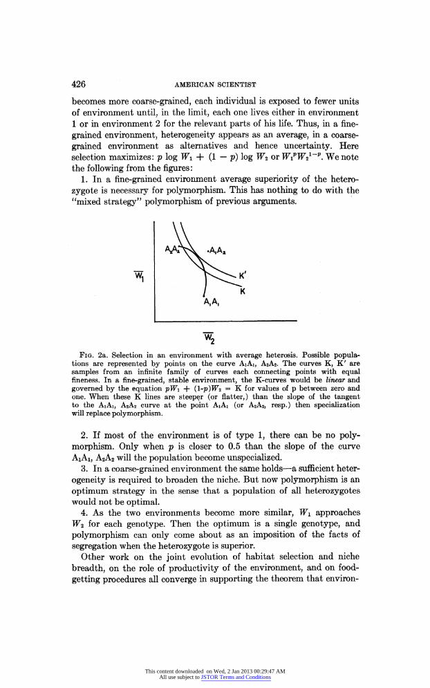
the following from the figures: 1. In a fine-grained environment average superiority of the hetero

zygote is necessary for polymorphism. This has nothing to do with the "mixed strategy" polymorphism of previous arguments.

Fig. 2a. Selection in an environment with average heterosis. Possible popula tions are represented by points on the curve AiAi, A2A2. The curves , K' are

samples from an infinite family of curves each connecting points with equal fineness. In a fine-grained, stable environment, the K-curves would be linear and

governed by the equation pW\ + (l-p)W<i = for values of between zero and

one. When these lines are steeper (or flatter,) than the slope of the tangent to the A1A1, A2A2 curve at the point A1A1 (or A2A2, resp.) then specialization will replace polymorphism.

2. If most of the environment is of type 1, there can be no poly morphism. Only when is closer to 0.5 than the slope of the curve

A1A1, A2A2 will the population become unspecialized. 3. In a coarse-grained environment the same holds?a sufficient heter

ogeneity is required to broaden the niche. But now polymorphism is an

optimum strategy in the sense that a population of all heterozygotes would not be optimal.

4. As the two environments become more similar, Wi approaches W2 for each genotype. Then the optimum is a single genotype, and

polymorphism can only come about as an imposition of the facts of

segregation when the heterozygote is superior. Other work on the joint evolution of habitat selection and niche

breadth, on the role of productivity of the environment, and on food

getting procedures all converge in supporting the theorem that environ




mental uncertainty leads to increased niche breadth while certain but diverse environments lead to specialization.

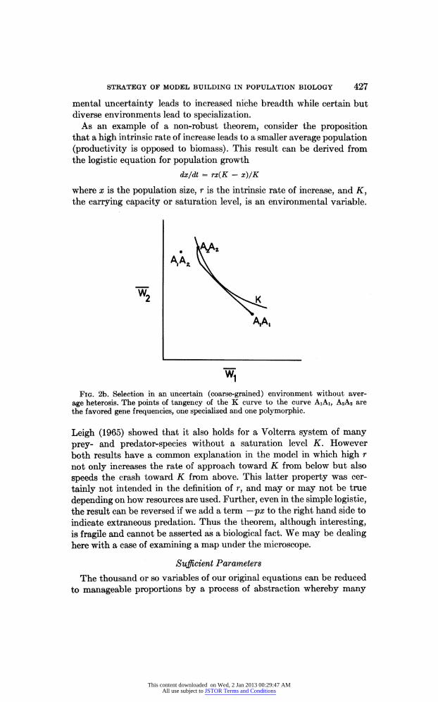
As an example of a non-robust theorem, consider the proposition that a high intrinsic rate of increase leads to a smaller average population (productivity is opposed to biomass). This result can be derived from the logistic equation for population growth

dx/dt = rx(K - x)/K

where is the population size, r is the intrinsic rate of increase, and K, the carrying capacity or saturation level, is an environmental variable.

Fig. 2b. Selection in an uncertain (coarse-grained) environment without aver

age heterosis. The points of tangency of the curve to the curve AiAi, A2A2 are

the favored gene frequencies, one specialized and one polymorphic.

Leigh (1965) showed that it also holds for a Volterra system of many

prey- and predator-species without a saturation level K. However

both results have a common explanation in the model in which high r

not only increases the rate of approach toward from below but also

speeds the crash toward from above. This latter property was cer

tainly not intended in the definition of r, and may or may not be true

depending on how resources are used. Further, even in the simple logistic, the result can be reversed if we add a term ?px to the right hand side to

indicate extraneous pr?dation. Thus the theorem, although interesting, is fragile and cannot be asserted as a biological fact. We may be dealing here with a case of examining a map under the microscope.

Sufficient Parameters

The thousand or so variables of our original equations can be reduced

to manageable proportions by a process of abstraction whereby many




terms enter into consideration only by way of a reduced number of

higher-level entities. Thus, all the physiological interactions of genes in a genotype enter the models of population genetics only as part of "fitness." The great diversity in populations appears mostly as "additive

genetic variance" and "total genetic variance." The multiplicity of

species interactions is grouped in the vague notions of the ecological niche, niche overlap, niche breadth, and competition coefficients. It is an essential ingredient in the concept of levels of phenomena that there exists a set of what, by analogy with the sufficient statistic, we can call sufficient parameters defined on a given level (say community) which are

very much fewer than the number of parameters on the lower level and which among them contain most of the important information about events on that level. This is by no means equivalent to asserting that

community properties are additive or that these sufficient parameters are independent.

Sometimes, the sufficient parameters arise directly from the mathe matics and may lack obvious intuitive meaning. Thus, Kerner dis covered a conservation law for predator-prey systems. But what is con

served is not anything obvious like energy or momentum. It is a com

plicated function of the species densities which may acquire meaning for us with further study. Similarly, working with cellular metabolism and starting like Kerner with a physics background, Goodwin (1963) found an invariant which he refers to metaphorically as a biological "temperature."

In other cases, the sufficient parameters are formalizations of pre viously held but vague properties such as niche breadth. We would like some measure of niche breadth which reflects the spread of a species' fitness over a range of environments. Thus the measure should have the

following properties: if a species utilizes resources equally, it should have a niche breadth of N. If it uses two resources unequally, the niche breadth measure should lie between 1 and 2. If two populations which have equal niche breadths that do not overlap are merged, their joint niche breadth should be the sum of their separate breadths. It may be less if they overlap but never more. Two measures satisfy these re

quirements :

log ? ?

log

where is the measure of relative abundance of the species on a given resource or in a given habitat, and

1/B = p2

Neither one is the "true" measure in the sense that one can decide between proposed alternative structures for the hemoglobin molecule. Both are defined by us to meet heuristic criteria. The final choice of an

appropriate measure of niche breadth will depend on convenience, on




some new criteria which may arise, and on the extent to which the measures lead to biological predictions based on niche breadth. Mean

while, we should use both measures in presenting ecological data so that

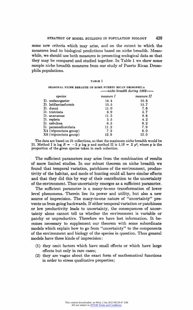
they may be compared and studied together. In Table 1 we show some

sample niche breadth measures from our study of Puerto Ric?n Droso

phila populations.

TABLE 1

SEASONAL NICHE BREADTH OF SOME PUERTO RIC?N DROSOPHILA ,-niche breadth during 1962???

species measure I measure II D. melanogaster 14.4 10.5 D. latifasciaeformis 15.5 15.7 D. dunni 11.0 7.6 D. tristriata 6.9 5.7 D. ananassae 11.2 8.6 D. repleta 5.5 4.2 D. nebulosa 6.5 6.2 D. paramediostriata 11.2 7.9 X4 (tripunctata group) 7.2 6.0 X6 (tripunctata group) 13.9 12.0

The data are based on 21 collections, so that the m?ximum niche breadth would be 21. Method I is log = ?

log and method II is 1/B ?

2, where is the proportion of the given species taken in each collection.

The sufficient parameters may arise from the combination of results of more limited studies. In our robust theorem on niche breadth we found that temporal variation, patchiness of the environment, produc tivity of the habitat, and mode of hunting could all have similar effects and that they did this by way of their contribution to the uncertainty of the environment. Thus uncertainty emerges as a sufficient parameter.

The sufficient parameter is a many-to-one transformation of lower level phenomena. Therein lies its power and utility, but also a new source of imprecision. The many-to-one nature of "uncertainty" pre vents us from going backwards. If either temporal variation or patchiness or low productivity leads to uncertainty, the consequences of uncer

tainty alone cannot tell us whether the environment is variable or

patchy or unproductive. Therefore we have lost information. It be comes necessary to supplement our theorem with some subordinate

models which explain how to go from "uncertainty" to the components of the environment and biology of the species in question. Thus general models have three kinds of imprecision :

(1) they omit factors which have small effects or which have large effects but only in rare cases;

(2) they are vague about the exact form of mathematical functions in order to stress qualitative properties;




(3) the many-to-one property of sufficient parameters destroys in

formation about lower level events.

Hence, the general models are necessary but not sufficient for under

standing nature. For understanding is not achieved by generality alone, but by a relation between the general and the particular.

Clusters of Models

A mathematical model is neither an hypothesis nor a theory. Unlike the scientific hypothesis, a model is not verifiable directly by experiment. For all models are both true and false. Almost any plausible proposed

Developmental biology

Measures of environmental

diversity

Response to selection in a heterogeneous environment

classical

^population genetics

Fig. 3. Relations among some of the components in a theory of the structure of an

ecological community. Broken lines enclose alternative equivalent models.

relation among aspects of nature is likely to be true in the sense that it occurs (although rarely and slightly). Yet all models leave out a lot and are in that sense false, incomplete, inadequate. The validation of a

model is not that it is "true" but that it generates good testable hy potheses relevant to important problems. A model may be discarded in

favor of a more powerful one, but it usually is simply outgrown when the live issues are not any longer those for which it was designed.




Unlike the theory, models are restricted by technical considerations to a few components at a time, even in systems which are complex. Thus a satisfactory theory is usually a cluster of models. These models are related to each other in several ways : as coordinate alternative models

for the same set of phenomena, they jointly produce robust theorems; as complementary models they can cope with different aspects of the same problem and give complementary as well as overlapping results; as hierarchically arranged "nested" models, each provides an interpre tation of the sufficient parameters of the next higher level where they are

taken as given. In Figure 3 we show schematically the relations among some of the models in the theory of community structure.

The multiplicity of models is imposed by the contradictory demands

of a complex, heterogeneous nature and a mind that can only cope with

few variables at a time; by the contradictory desiderata of generality,

realism, and precision; by the need to understand and also to control; even by the opposing esthetic standards which emphasize the stark

simplicity and power of a general theorem as against the richness and

the diversity of living nature. These conflicts are irreconcilable. There

fore, the alternative approaches even of contending schools are part of

a larger mixed strategy. But the conflict is about method, not nature, for the individual models, while they are essential for understanding

reality, should not be confused with that reality itself.

BIBLIOGRAPHY

1. Goodwin, . C. Temporal Organization in Cells. Academic Press 1963. 2. Holling, C. S. The components of pr?dation as revealed by a study of small

mammal pr?dation of the European pine sawfly. Canadian entomologist, 91 (5) 293

320, 1959. 3. Kerner, E. H. A statistical mechanics of interacting biological species. Bull. Mat.

Biophys., 19, 121-146, 1957. 4. Leigh, Egbert. On the relation between productivity, biomass, diversity, and

stability of a community. PN AS, 58 (4) 777-783, 1965. 5. Levins, R. Theory of fitness in a heterogeneous environment, I. The fitness set

and adaptive function. Am. Nat., 96 (891), 361-373, 1962.

6. Levins, R. and R. H. MacArthur. In press. 7. MacArthur, R. H. and R. Levins. Competition, habitat selection, and character

displacement in a patchy environment. PNAS, 51 (3) 1207-1210, 1965. 8. Watt, Kenneth E. F. The choice and solution of mathematical models for pre

dicting and maximizing the yield of a fishery. /. Fisheries Ees. Bd. of Canada, 13,

613-645, 1956.



levins 1966 strategyecologymodels

Documents

population ecology

population genetics

population biologyauthors

population density

single population

jstor terms

jstor archive

mathematical model