University of Limerick

Liam Mescall

The Application of the Nelson Siegel Model to European

Corporate CDS Curves

M.Sc. in Computational Finance

2011

University of Limerick

M.Sc in Computational Finance

Date of Submission: September 5th, 2011

Name: Liam Mescall

ID Number: 0144126

Word Count: 9,162

Supervisor: Dr. Finbarr Murphy

This dissertation is the sole work of the author and

submitted in partial ful�llment of the requirements of the

M.Sc. in Computational Finance.

ii

Abstract

Bond market growth over the past century has encouraged the construction of

numerous models capable of calculating a term structure of interest rates. In

1987, Nelson and Siegel produced a paper that produced one such term struc-

ture. Risk exposure to credit markets have witnessed change with the invention

of the credit default swap (CDS) in 1994. This allowed for hedging / specu-

lating of / on credit risk of a particular underlying corporate or sovereign. We

consider approaches to interest rate term structure calculation to be compa-

rable to that of a CDS term structure with both requiring the payment of a

�xed, predetermined amount on �xed dates. This paper applies the model con-

structed by Nelson and Siegel to a selection of European Corporate CDS's term

structures, analyzes the three elements of the model and their implications for

the credit asset class before drawing conclusions and o�ering further points of

research stemming from the results. Testing is performed on 117 entities form

the iTraxx Europe index over the period July, 2008 to April, 2009.

While the results are mixed in certain sectors, generally our �ndings show

the inability of the model to completely deal with the volatility noted along

the term structure of CDS yields. Over the testing period, CDS curves proved

extremely volatile with frequent non parallel shifts in response to macroeconomic

events. However, measures could be taken to further tailor the model to the CDS

curve shapes. We believe the interpolation of the credit curve (eight points) to

replicate the number of data points used in the Nelson and Siegel paper (thirty

points) would smooth the curve removing a signi�cant portion of the volatility.

Also, the introduction of the Svensson (1994) adjustment, which allows for the

modeling of a second hump / trough variable, would cater towards the changing

shapes of the CDS curves.

iii

Following the application of these changes we suggest further research that

will develop these �ndings through the prediction of CDS term structures by

predicting the model parameters as individual time series. This has been com-

pleted with notable success in subsequent papers.

iv

Acknowledgments

Thanks to my supervisor, Dr. Finbarr Murphy, for the continued support

and guidance over the past year which has made this thesis an interesting and

bene�cial experience.

v

Contents

1 Introduction 1

1.1 Introduction . . . . . . . . . . . . . . . . . . . . . . . . . . . . . . 1

2 Literature Review 3

2.1 Introduction . . . . . . . . . . . . . . . . . . . . . . . . . . . . . . 3

2.2 Challenges to Term Structure Construction . . . . . . . . . . . . 4

2.3 How the Model Calculates Term Structures . . . . . . . . . . . . 6

2.4 τ Parameter . . . . . . . . . . . . . . . . . . . . . . . . . . . . . . 9

3 Methodology 12

3.1 CDS Valuation . . . . . . . . . . . . . . . . . . . . . . . . . . . . 12

3.2 Comparing Asset classes . . . . . . . . . . . . . . . . . . . . . . . 13

3.3 Fitting an Interest Rate Curve . . . . . . . . . . . . . . . . . . . 14

4 Data 17

4.1 Data Description . . . . . . . . . . . . . . . . . . . . . . . . . . . 17

4.2 Trends in Data . . . . . . . . . . . . . . . . . . . . . . . . . . . . 18

4.3 Descriptive Statistics . . . . . . . . . . . . . . . . . . . . . . . . . 21

4.4 Normality of Returns Generated by Sector . . . . . . . . . . . . . 22

5 Results 23

5.1 Analysis of τ Parameter . . . . . . . . . . . . . . . . . . . . . . . 23

5.1.1 Impact of Changing τ Parameter . . . . . . . . . . . . . . 25

5.2 Multicollinearity . . . . . . . . . . . . . . . . . . . . . . . . . . . 27

5.3 Analysis of Level Parameter . . . . . . . . . . . . . . . . . . . . . 27

5.4 Analysis of Slope Parameter . . . . . . . . . . . . . . . . . . . . . 30

5.5 Analysis of Curvature Parameter . . . . . . . . . . . . . . . . . . 32

5.6 Parameter Correlation Analysis . . . . . . . . . . . . . . . . . . . 35

vi

6 Economic Interpretation 37

6.1 τ Parameter . . . . . . . . . . . . . . . . . . . . . . . . . . . . . . 37

7 Conclusion 40

7.1 Main Findings . . . . . . . . . . . . . . . . . . . . . . . . . . . . 40

7.2 Further Research . . . . . . . . . . . . . . . . . . . . . . . . . . . 41

7.3 Concluding Remarks . . . . . . . . . . . . . . . . . . . . . . . . . 42

8 Appendices 43

9 Bibliography 63

vii

List of Figures

Figure

No. Title Page

1 Nelson Siegel Forward Rate Curve - Beta Parameters 8

2 Nelson Siegel Spot Rate Curve - Beta Parameters 9

3 Nelson Siegel Forward Rate Curve - Tau Parameter 10

4 Nelson Siegel Spot Rate Curve - Tau Parameter 10

5 Nelson Siegel Approximation Example 15

6 Credit Curves on July 18th, 2008, Re-based to 1 18

7 Credit Curves on July 18th, 2008, Re-based to 1 19

8 Residuals on July, 18th, 2008 20

9 Residuals on July 18th, 2008 21

10 Nelson Siegel Curves with Di�ering Tau Values 23

11 NS Curve Best Fit Tau Compared to Median Tau 26

12 Change in Volvo Curve Between 5-12-2008 & 12-12-2008 29

13 Change in Total Curve Between 12-12-2008 & 19-12-2008 30

14 Change in Daimler Curve Between 2-1-2009 & 9-1-2009 32

15 Change in United Curve Between 10-10-2008 & 17-10-2008 33

16 Change in Unilever Curve Between 12-9-2008 & 19-9-2008 34

17 Change in Koninkluke Curve Between 9-1-2009 & 16-1-2009 35

18 Tau Time-line over Testing Period 38

viii

List of Tables

Table

No. Title Page

1 Distribution of Tau per Sector 25

2 Market Observed and NS Observed Level Correlation 28

3 % Change in Curves 29

4 % Change in Curves 30

5 Market Observed and NS Observed Slope Correlation 31

6 Market Observed and NS Observed Curvature Correlation 33

7 CDS Curve Level 36

8 CDS Curve Slope 36

9 CDS Curve Curvature 37

ix

1 Introduction

1.1 Introduction

Yield curve �tting can be traced back to 1942 and the pioneering work of

David Durand who sketched lines amongst a scatter plot of yields, in a sub-

jectively reasonable way, attempting to identify a possible term structure of

interest rates (Durand (1942)). Successful construction was limited until the

late seventies when research focusing on the economic impact of money demand

was presented. This, coupled with an ever growing �xed income market encour-

aged academics to create a parsimonious model with the ability to represent the

typically observed; monotonic, humped and S shaped curves in a term struc-

ture of interest rates (Friedman (1977)). In 1987 Charles Nelson and Andrew

Siegel developed one such model. The Nelson Siegel (NS) model is a three fac-

tor model which achieves this �exible curve �tting through the transformation

of bond yields to zero coupon bond prices before using regression to estimate

the level, slope and curvature of the yield curve (Nelson and Siegel (1987)).

The model, and models stemming from it, have been widely used over the past

twenty years in creating term structure forecasts for central banks and other

market participants (Bank of International Settlements (2005)).

In 1994 a new form of credit derivative security was created, the credit

default swap (CDS). This insurance product allows investors to o�set portions

of risk assumed from the purchase of debt in a particular company in exchange

for a periodic payment, calculated as a percentage of the notional. Prices are

quoted in premia over a �xed period of time with the varying maturities giving

rise to a curve, similar to that of the interest rate curve. Once a CDS contract is

entered into, the buyer (short credit of underlying) is obliged to make �xed rate

payments periodically to the seller (long credit of the underlying) until maturity.

1

The holder of the CDS contract retains the right to sell a particular bond issued

by the company for its par value should a credit event1 occur. While initially

constructed as a risk management tool, the appeal to investors of an exposure

to the pure creditworthiness of a company / sovereign has contributed to global

CDS markets expanding from USD $5 bn dollars in 1994 to USD $25.5 trillion

dollars by the end of 20102.

Noting equivalence between the credit and interest rate security curves, we

propose to further employ this model in the analysis of European corporate

credit default swaps by subjecting their credit curves to analysis similar to the

1987 Nelson and Siegel paper. Results will be explored in light of the di�erences

between the two asset classes and the ability of the model to analyze a CDS

term structure using the three parameters generated by the model.

1As de�ned by ISDA documentation. See www.isda.org for same.2Source:ISDA. See www.isda.org

2

2 Literature Review

2.1 Introduction

In the absence of literature and research analyzing the application of �xed

income models to CDS analysis, this literature review will focus on a review of

the NS paper itself, the challenges observed from previous papers, a discussion

of subsequent papers based on the model and an overview of the elements of

the model that contribute to term structure calculation.

Seeking to investigate traditional expectations theory and Wood's (1983)

observations that yield curves over time present the long term shape of yield

curves to be either monotonic, humped or S-shaped, Nelson and Siegel (1987)

developed an equation capable of generating a series of forward rate curves

dependent on the level, slope and curvature variables that describe a curve.

The model was developed noting the generation of spot rates from a di�erential

equation can be solved by forward rates (as forecasts). The yield to maturity

is then calculated as the average of these forward rates. Testing of this model

was based on the U.S. Treasury yield curve over the period January 1981 to

October 1983. To avoid complications, such as di�ering taxation rates, zero

coupon bonds were used as the preferred bond type. Zero coupon bond prices

are calculated based on the zero coupon yields noted on the curve. These prices

are then used to calculate the continuously compounded rate of return from

delivery to maturity based on an annualized 365.25 year, providing the required

data to �t the curve to the model. Using ordinary least squares (OLS), the curve

is then �tted to the model. The completion of this process over thirty seven

periods produced an average R2value of .959 demonstrating their model was

capable of capturing a variety of observed yield curve shapes over time (Nelson

and Siegel (1987)). Nelson and Siegel then use these model results to forecast

3

future yield curves, something that is beyond the scope of this paper. Instead,

this paper chooses to analyze the level, slope and curvature components of the

model for the credit asset class with comparisons made to the original interest

rate yield curve.

2.2 Challenges to Term Structure Construction

Literature identi�es challenges presented during term structure construction

which may further aid analysis of the credit asset class:

1. Fitting accuracy is forgone for the sake of simplicity. This is clearly inten-

tional as is stated on page 479 of the Nelson and Siegel (1987) paper,�...no

set of values of the parameters would �t the data perfectly, nor is it our

objective to �nd a model that would do so�. Also, the paper cites the

absence of continuous trading in bills and securities selling at premia /

discounts as a result of transaction costs as potentially distorting testing.

These are potential data issues for the credit asset class also.

2. The NS model adopts a two step approach which iterates on one parameter

then estimates the values that will best �t to the other three parameters

using OLS regression. This requires at least four points as there are four

parameters increasing the data requirements of the process. Spline models

can �t yield curves with far more accuracy and with as little as two points.

3. The iterative nature and data requirements described above increases the

complexity and labor intensity of the process. This is not required in other

interest rate calculations.

4. The model appears inconsistent with arbitrage free term structure models

(Filipovic (1999)). The practical implications of this are the potential for

4

existence of a portfolio consisting of both long and short positions that

will generate pro�t with zero risk. The pro�t noted is nothing less than

the observed error terms in the NS model. This is intuitively incorrect.

5. We note from Hurn, Lindsay and Palov (2005) that there is a concentration

of sensitivity in one variable, τ , which represents the time in years and

e�ectively determines the shape of the curve. De Pooter (2007) also notes

the τ variable cannot handle the complete set of shapes the curve takes

over longer periods of time.

6. The high degree of correlation between the factors in the NS model make it

di�cult to estimate the parameters correctly (multicollinearity) (Diebold

and Li (2006)). These correlations are a�ected by the τ value as illustrated

in Annaert et al (n.d.) who compared long and short time to maturity

vectors and showed shorter maturities are more sensitive. This means the

higher correlations at the short end make parameters harder to calculate.

Ridge regression and other spline techniques have been implemented to

overcome this.

The model has been extended to address some of these �ndings. Diebold and

Li (2006) vary the model by estimating autoregressive models for the factors

(level, slope and curvature) and then forecasting the yield curve by forecasting

the factors. This has produced sizable increases in accuracy of one-year-ahead

predictions. Further �exibility in the model was introduced by Svensson (1994)

through the introduction of an additional hump position in the spot rate curve.

Gauthier and Simonato (2009) introducing yet another parameter to control the

curves sensitivity to this hump. These adaptations still share the collinearity

problem outlined above. Litterman and Scheinkman (1991) employ the concept

of level, slope and curvature to hedge interest rate risk by considering the e�ect

5

of each factor on the portfolio as collectively they explain almost all variation

across the various maturities. Dullmann and Uhrig-Homburg (2000) estimate

the interest rate risk structure for Deutschmark denominated bonds on a va-

riety of Moody's rating categories. This allowed them to conclude the rating

system does not provide su�cient information as to the quality of the issue and

bond prices are a�ected by many factors not accounted for by typical models.

Martinellini and Meyfredi (2007) use the model to approximate the time vary-

ing parameters a�ecting the shape of the yield curve before employing a copula

approach to value at risk calculations.

The overall accuracy of the NS model has been observed to perform well

over the longer term following benchmarking tests performed by Fabozzi et al

(2005) and Diebold and Li (2006) on adjusted models. These successes account

for its continued popularity and use by central banks around the world (Bank

of International Settlements (2005)).

2.3 How the Model Calculates Term Structures

The ability of the model to create the variety of shapes previously described

can potentially deliver similar results to the Nelson and Siegel 1987 paper. The

forward rate model developed is as follows:

r(m) = β0 + β1.exp(−m/τ) + β2[(m/τ).exp(−m/τ)] (1)

To obtain yield as a function of maturity, model (1) integrates R(�) from zero

to m and divides by m producing equation (2). By splitting the RHS of (2)

into three parts we can analyze the components of the model. β0 contributes

the long term component and is considered the long term interest rate. It is a

6

constant that does not decay to zero as other beta values do. β1 and its loading

[1− exp(−mτ )]/(m/τ) is the short term component which contributes the slope

factor. It decays monotonically and quite rapidly towards zero. If β1 > 0 then

there will be a downward sloping curve or upwards when 0 > β1. β2 and its

loading[exp(−mτ )

]represents the medium term component and contribute the

degree of curvature, the higher its value, the higher the degree of curvature

in the hump/trough. Diebold and Li (2006) note that an increase in β1 will

increases short yields more than long yields, as short rates load more heavily

causing changes in the shape of the yield curve. These parameters are estimated

through the use of OLS regression. The range of shapes the curve can take is

dependent on a single parameter, τ , which represents the rate at which the

regressor decays to zero. Nelson and Siegel (1987) note that small values of τ ,

which have rapid decay in regressors, tend to �t low maturities quite well with

larger values more appropriate to longer maturities. The τ that generates the

greatest R2 are chosen as the best �tting. Yield to maturity is described by:

R(m) = β0 + β1.[1− exp(−m/τ)]/(m/τ)− β2.exp(−m/τ) (2)

A variety of curves are produced based on the changing of the shape parameter,

τ . Ordinary least squares regression is then performed based on the selected τ

value to identify the best �tting parameters (Diebold and Li (2006)). By �xing

the τ value, the regression can be performed with one conditional variable which

changes a nonlinear estimation problem into a simple linear problem. The NS

model estimates its parameters by minimizing the sum of the squared errors over

a predetermined grid of τ values (Nelson and Siegel (1987)). Linear regression is

preferred as non linear introduces an extremely sensitive starting value as seen

in Cairns and Pritchard (2001). The parameters are graphically illustrated in

�gure 1 and 2 below as a function of time.

7

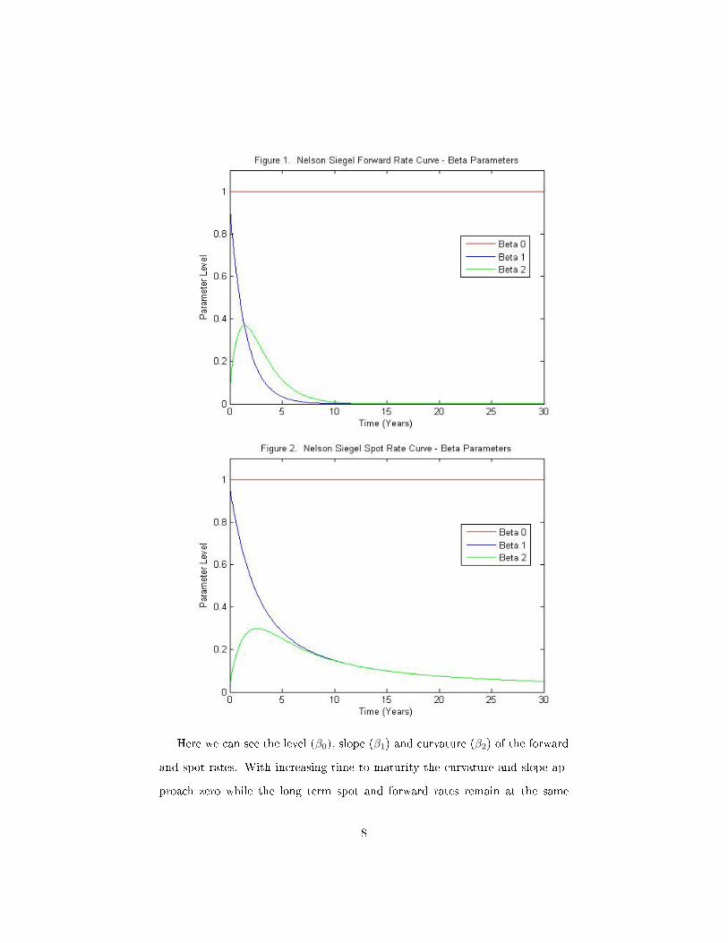
Here we can see the level (β0), slope (β1) and curvature (β2) of the forward

and spot rates. With increasing time to maturity the curvature and slope ap-

proach zero while the long term spot and forward rates remain at the same

8

constant rate, given by β0. We interpret the β0 level to be close to the long

term spot rate and assume to be non-negative.

As time to maturity approaches zero, the curvature (β2) and the slope noted

in the forward rate curve are more pronounced than the comparative spot rate

illustrating the greater speed of change over time.

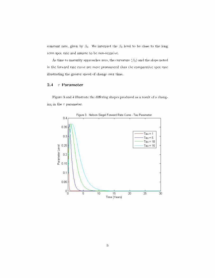
2.4 τ Parameter

Figure 3 and 4 illustrate the di�ering shapes produced as a result of a chang-

ing in the τ parameter.

9

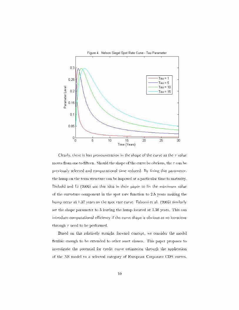
Clearly, there is less pronounceation in the shape of the curve as the τ value

moves from one to �fteen. Should the shape of the curve be obvious, the τ can be

previously selected and computational time reduced. By �xing this parameter,

the hump on the term structure can be imposed at a particular time to maturity.

Diebold and Li (2006) use this idea in their paper to �x the maximum value

of the curvature component in the spot rate function to 2.5 years making the

hump occur at 1.37 years on the spot rate curve. Fabozzi et al. (2005) similarly

set the shape parameter to 3 leaving the hump located at 5.38 years. This can

introduce computational e�ciency if the curve shape is obvious as no iterations

through τ need to be performed.

Based on this relatively straight forward concept, we consider the model

�exible enough to be extended to other asset classes. This paper proposes to

investigate the potential for credit curve estimation through the application

of the NS model to a selected category of European Corporate CDS curves.

10

The �tted curves will be decomposed into their level, slope and curvature and

analyzed in comparison to initial curve observations. Analysis of the τ variable

and macroeconomic events during the period will enable us to conclude on the

models ability to capture events in the real world. Should the model be deemed

suitable for the credit asset class then we suggest some further research, as noted

from Diebold and Li 2006 paper.

Considering the scale of the market and continued volume of trading, devel-

opments in analysis of securities will be of interest to the larger �nancial com-

munity including; investors seeking to buy and hold protection, portfolio man-

agers who wish to accurately hedge risk generated from corporate or sovereign

bonds held, regulators analyzing the exposures of institutions invested in credit

derivatives and those seeking to analyze CDS valuation through traditional �xed

income models.

Having introduced the model and its workings, the methodology will intro-

duce some traditional CDS valuation theory, develop a comparison of the CDS

and interest rate curves before discussing the application of the CDS curves to

the interest rate developed NS model. The fourth section describes the data set

chosen for testing, trends emerging in the data, the rational for their choice and

the time frame over which they will be tested. In chapter �ve we analyze the

results of the testing performed on the τ variable and each of the parameters.

An economic interpretation of the results then o�ers practical insight into the

meaning we can draw from the testing (chapter 6). Finally, chapter seven, con-

cludes on our �ndings and o�ers areas for further research based on this papers

�ndings.

11

3 Methodology

3.1 CDS Valuation

CDS prices are quoted in premia, which for one period can be calculated as:

s = p(1−RR) (3)

where s is the spread / premium, p is the probability of default and RR is

the recovery rate. Typical methods of valuing a CDS require the calculation

of default probabilities and recovery rates. The probability of default is often

inferred from bonds issued by the reference entity and based on the assumption

that the single reason a corporate bond will yield more than an equivalent risk

free treasury is the risk of default. These, like the probability of default, can

be subjective. Take a three-year zero coupon Treasury that yields 2% and a

comparable three-year corporate bond that yields 2.5%. Today's value of the

cost of the default is

100e−.02x3 − 100e−.025x3 = 1.402

If we assume there will be a zero recovery rate then we can solve:

100p(e−.02x3) = 1.402

for the p value producing a 1.48% risk neutral default probability in that period.

In practice recovery rates are non zero (leading to assumptions as to its value)

and corporate bonds seldom have zero coupons. A more detailed exposition of

CDS valuation can be found in Hull and Whites (2000) paper,�The Valuation

of Credit Default Swaps�. Assuming corporate bond prices are lower than Trea-

12

suries is solely due to the presence of credit risk excludes factors such as market

sentiment and the often lagged analysis of credit rating agencies. Similarly, re-

covery rates are based on perception of what the companies bonds will be worth

following a credit event, this is not an exact science.

3.2 Comparing Asset classes

As we are presented with two di�erent asset classes, the ability of the model

to replicate the success enjoyed by Nelson and Siegel (1987) with interest rate

curves will depend on the extent similarities exist between the asset classes. We

have observed interest rate and credit curves exhibit the following characteris-

tics:

1. Both curves can potentially take on monotonic, humped or S-shaped term

structures with a typical curve being increasing and concave.

2. Both describe yields paid at �xed intervals over a predetermined period

of time (assuming no credit event).

3. Both are leading economic indicators and a re�ection of the �nancial

health of an entity/sovereign.

4. Interest rate curves are signi�cantly more sensitive at the shorter end of

the curve with greater than two year terms typically a function of growth

and in�ation expectations. We consider CDS prices to be driven by the

entities ability to meet debt repayment falling due with the short end

similarly prone to more volatility than the long end.

5. Long rates are more persistent than short rates over time.

6. Typically, both curves are increasing and concave.

13

3.3 Fitting an Interest Rate Curve

The following are the steps used to develop a interest rate Nelson Siegel

curve:

1. Bonds at varying maturities are selected and payment dates identi�ed for

interest (if coupon bearing) and principal amounts.

2. Time is converted to decimal depending on appropriate day count conven-

tion i.e. payments at ninety 90 day intervals are represented by 90/360 =

.25 if the 360 day day count convention is adopted.

3. Initial parameters are identi�ed and input to formula (2) in section 2.3

above.

4. Yield curve values are calculated based on these parameters for all dates

identi�ed in second step.

5. Taking these yields and time in decimal, calculate zero bond prices based

on the following formula:

p(t) = exp−y(t)t (4)

6. Then, calculate the discounted value of each bond by multiplying the sum

of bond cash-�ows (if coupon bearing) and the current zero prices.

7. Compute the total of the squared price errors for all bonds.

8. Choose the best �tting parameter values by minimizing the sum of the

squared errors.

14

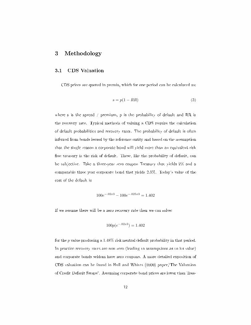
This process is best illustrated through an example. Figure 5 displays the

National Grid Plc CDS data points as of July 18th, 2008 along with a �tted

curve. The NS curve observed is one of many created by the model, each varying

with a change of τ value. It is preferred to the other curves as it represents the

lowest squared pricing error.

This curve will then be analyzed in terms of its parameters i.e. β0, β1, β2

and τ which are also outlined in the above graph. Time series analysis of these

15

parameters will be performed over the forty week period in the data section.

For the purposes of our testing we have set the range of τ values from zero to

3,650 which represents the range of days in the ten year period. By identifying

patterns in the parameters we hope to gain insight into the ability of the NS

model to model the credit asset class.

16

4 Data

4.1 Data Description

The data set to test the application of the NS model is taken from 117

companies listed in the Markit iTraxx European listing. These are spread across

�ve sectors including;

1. Auto and industrial.

2. Consumer.

3. Energy.

4. Financial.

5. Technology, media and telecommunication (TMT).

We have chosen a period which includes the collapse of Lehman Brothers and

the Russian �nancial crisis. During this period credit market volatility increased

above normal levels. We expect this volatility to create monotonic, humped and

S shaped curves, testing the model. The curves will be �tted to the Nelson Siegel

model for every Monday between July 18th, 2008 and April 17th, 2009 totaling

forty period for each of the 117 entities. β and τ parameters for each curve will

be calculated to facilitate analysis of curve parameters compared to initial curve

observations. Time series analysis will be used to identify patterns relative to

macroeconomic events and highlight times the model cannot model the credit

asset class. We consider the testing of 4,680 individual curves across this variety

of industries su�cient to give statistical signi�cance to our results.

17

4.2 Trends in Data

As we have such a diverse population of credit curves, it is important to

understand their general structure. To illustrate how the curves evolve relative

to each other and identify any trend emerging from the population of credit

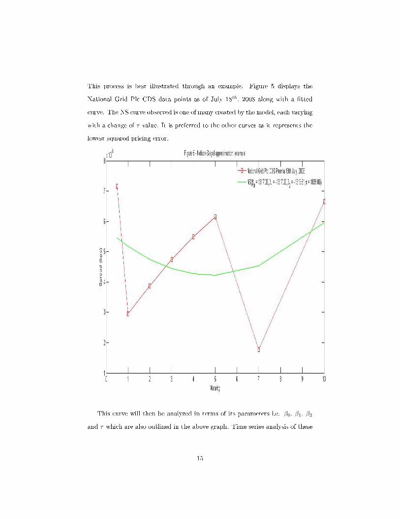
curves, we have rebased all curves to one. Figures 6 and 7 below o�er two views

of the same dataset at the same point in time, the �rst curve on the �rst date

of the testing period, July 18th, 2008:

A number of patterns emerge from Figure 6. With the exception of the

energy sector curves (from 58 to 77), which slope monotonically upwards, the

18

vast majority of companies have a higher six month spread than one and two

year spreads re�ecting the �nancial crisis at the time.

The curves �uctuate broadly at the six month spread level (excluding energy

sector) with most curves recording two or more hump / trough features. The

trend in energy sector curves is surprising as the companies listed (see Appendix

1) generate revenues from energy consumption on a global scale. At this point

the worlds short term economic outlook was bleak suggesting lower consumption

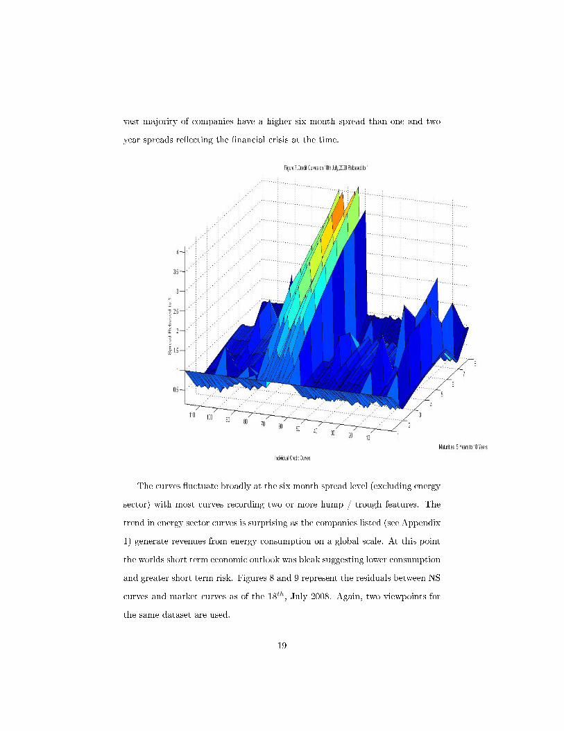
and greater short term risk. Figures 8 and 9 represent the residuals between NS

curves and market curves as of the 18th, July 2008. Again, two viewpoints for

the same dataset are used.

19

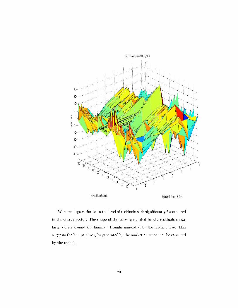
We note large variation in the level of residuals with signi�cantly fewer noted

in the energy sector. The shape of the curve generated by the residuals shows

large values around the humps / troughs generated by the credit curve. This

suggests the humps / troughs generated by the market curve cannot be captured

by the model.

20

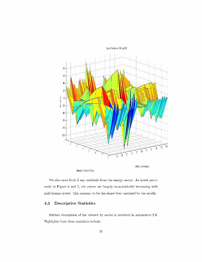
We also note little if any residuals from the energy sector. As noted previ-

ously in Figure 6 and 7, the curves are largely monotonically increasing with

mild humps noted. This appears to be the shape best captured by the model.

4.3 Descriptive Statistics

Further description of the dataset by sector is provided in appendices 2-6.

Highlights from these statistics include:

21

1. Standard deviations are lower than mean curve values in all but the auto

and industrial sectors which are on average 30 % higher than the mean at

each maturity.

2. The mean, standard deviation, minimum and maximum spreads noted at

each maturity are quite similar for respective sectors at each maturity.

This re�ects the steepening at the short end and further highlights the

�attening of the curves during the period.

3. The average auto and industrial curves are substantially higher than each

of the other four sectors re�ecting a perceived decline in consumption.

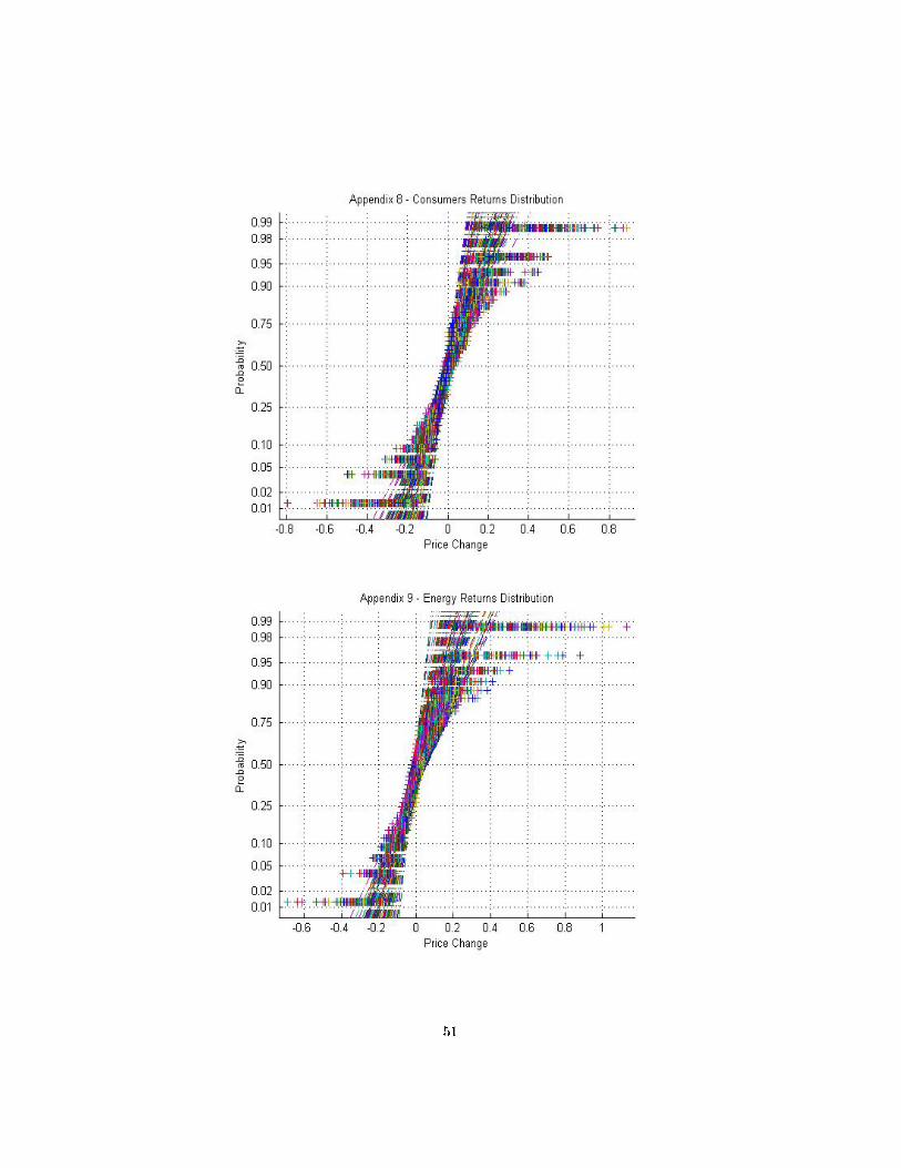
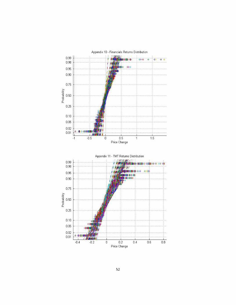
4.4 Normality of Returns Generated by Sector

To illustrate the volatility in curve levels over the forty week period we have

graphed the percentage returns relative to a normal distribution of returns. Re-

fer appendices 7 - 11 for same. The �nancial sector produces the most normally

distributed returns (Appendix 10) with consumers and auto and industrials

both producing the most return outliers (Appendices 7 and 8) and suggesting

greater intraday volatility. Financial sector returns are surprising considering

the period of testing contains the collapse of Lehman Brothers.

22

5 Results

5.1 Analysis of τ Parameter

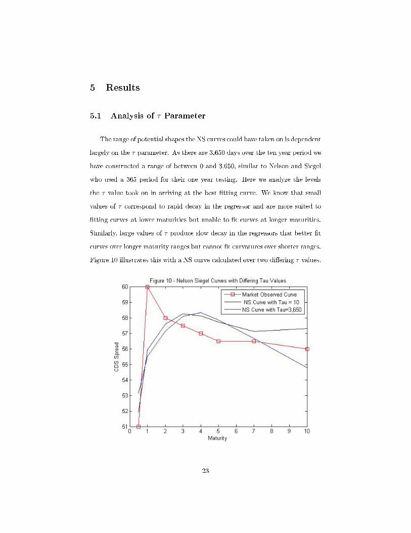
The range of potential shapes the NS curves could have taken on is dependent

largely on the τ parameter. As there are 3,650 days over the ten year period we

have constructed a range of between 0 and 3,650, similar to Nelson and Siegel

who used a 365 period for their one year testing. Here we analyze the levels

the τ value took on in arriving at the best �tting curve. We know that small

values of τ correspond to rapid decay in the regressor and are more suited to

�tting curves at lower maturities but unable to �t curves at longer maturities.

Similarly, large values of τ produce slow decay in the regressors that better �t

curves over longer maturity ranges but cannot �t curvatures over shorter ranges.

Figure 10 illustrates this with a NS curve calculated over two di�ering τ values.

23

We can see the more pronounced black line forming a better �t to the volatile

short end of the curve but tapering o� at the later maturity. Surprisingly there

is not a greater di�erence given the di�erence in τ values.

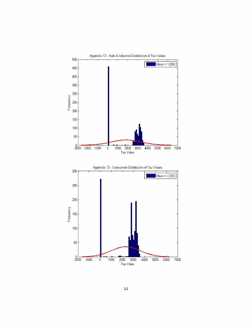
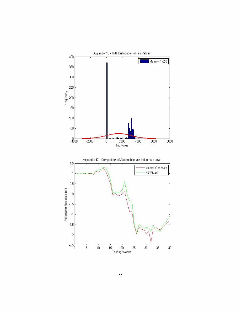
Appendices 12 - 16 graphically illustrate τ distribution by sector. From these

graphs we can see that no sector has a concentration of values around its mean

with the majority of values noted at the outer limits of the range. Table 1 o�ers

further insight into this distribution. With 28% of the range accounting for 74%

of τ values it is clear that the curves are better �tted at the extremities of the

range.

Table 1. Distribution of Tau per Sector

Sector Between 0 - 500 Between 3000 - 3650

Auto & Industrial 40% 36%

Consumers 24% 40%

Energy 59% 17%

Financial 18% 48%

TMT 49% 31%

Annaert et al observe two explanations for the large grouping of shape pa-

rameter in the upper bound of the range; the absence of a hump/trough or the

presence more than one hump/trough. In the absence of a hump/trough the

optimization procedure estimates the hump to be at the very end of the term

structure. Curves without a hump/trough can be more accurately modeled by

the NS model when the curvature component is dropped, a method also advo-

cated by Nelson and Siegel. Application of this adjusted model may be best

suited to the energy sector as Table 1 shows 76% of its τ values are captured

in its extremities. This will also eliminate the potential multicollinearity issue

(see 5.1.2).

24

The presence of more than one hump/trough is too complicated to be de-

scribed by the NS model. Instances of more than one hump/trough are best

modeled by introducing the Svensson (1994) adjustment which adds a second

hump/trough term to the NS model. It appears the NS model cannot accurately

model this volatility raising questions as to the initial claims of a �exible model

that can capture the movement in S shaped curves. The large grouping of shape

parameters between zero and 500 re�ect the curve pronouncement at the short

end similar to the example in Figure 10 where smaller values of τ provided a

far greater �t to the curve.

The period of testing noted huge stress in credit markets and persistent

volatility in the lead up to, and collapse of, Lehman Brothers which saw many

curves taking on two or more humps/troughs. This generally caused curves at

the shorter end to spike amid growing uncertainty as to the health of the world

economy. The variability of these term structures is highlighted in Figures 6

and 7. While on average there is signi�cant volatility over the curves, the low

τ value suggests volatility is greater at the short end. This seems appropriate

considering the shock to the world economy at the time.

5.1.1 Impact of Changing τ Parameter

Nelson and Siegel observe varying values of τ within results but also note

little loss of precision of �t if the median τ value is imposed. Testing a sample

of twenty curves across all sectors our �ndings are consistent noting little loss

of accuracy when replaced with the median value.

25

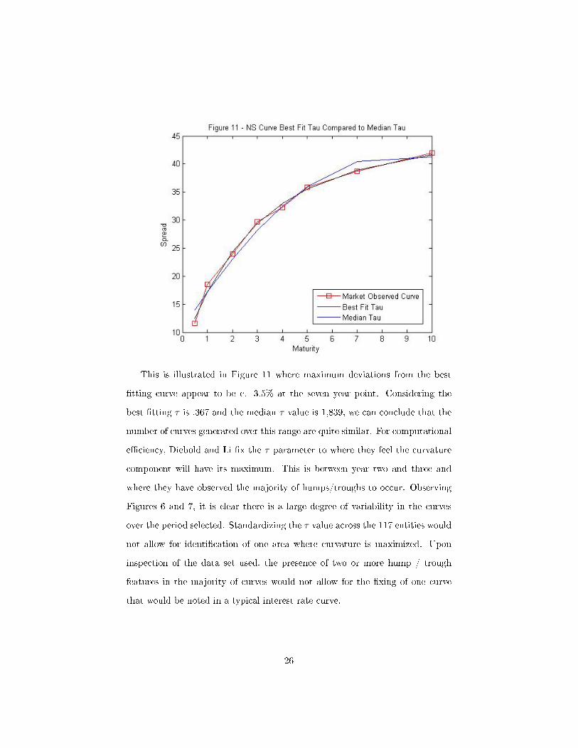
This is illustrated in Figure 11 where maximum deviations from the best

�tting curve appear to be c. 3.5% at the seven year point. Considering the

best �tting τ is .367 and the median τ value is 1,839, we can conclude that the

number of curves generated over this range are quite similar. For computational

e�ciency, Diebold and Li �x the τ parameter to where they feel the curvature

component will have its maximum. This is between year two and three and

where they have observed the majority of humps/troughs to occur. Observing

Figures 6 and 7, it is clear there is a large degree of variability in the curves

over the period selected. Standardizing the τ value across the 117 entities would

not allow for identi�cation of one area where curvature is maximized. Upon

inspection of the data set used, the presence of two or more hump / trough

features in the majority of curves would not allow for the �xing of one curve

that would be noted in a typical interest rate curve.

26

5.2 Multicollinearity

Multicollinearity describes the extent two or more variables in a regression

model are highly correlated. Diebold and Li (2006) consider its presence an

obstacle to accurately estimating parameters. This becomes a problem when

using parameters to predict terms structures as the greater the presence of mul-

ticollinearity; the higher the observed standard error, the larger the con�dence

intervals and smaller the t-statistics. Also, its presence can cause instability of

the regression coe�cients (Annaert et al). Observing parameter results, we note

a high degree of multicollinearity.

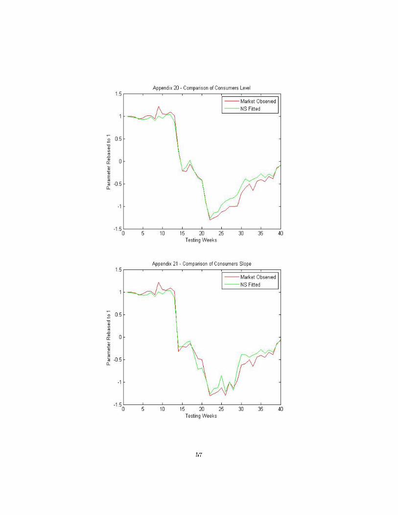
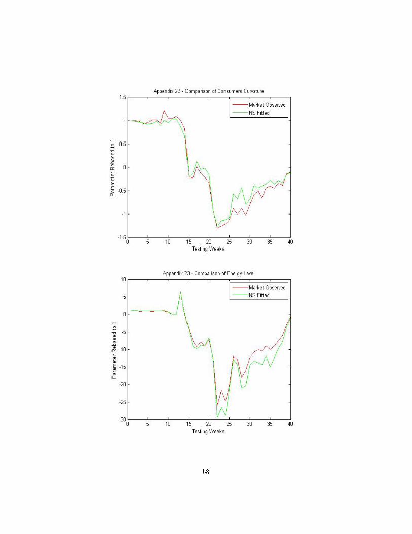
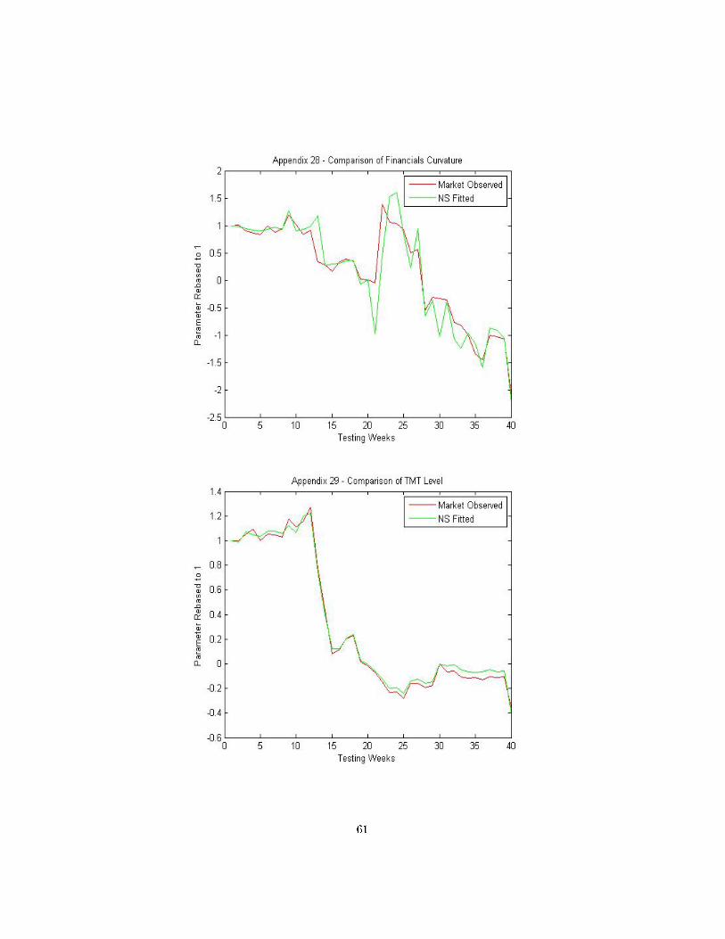
5.3 Analysis of Level Parameter

Residuals are further investigated by deconstructing the model into level,

slope and curvature components of both the market observed curves and NS

curves. A time series for each is calculated over the forty week period. Appen-

dices 17, 20, 23, 26 and 29 graphically illustrate the level parameter in each of

the sectors. A speci�c level parameter is generated for each curve i.e. Figure

10 exhibits curves with di�ering levels. We have constructed the average curve

parameter across each sector. Table 2 details the level correlations.

Table 2.

Market Observed and NS Observed Level Correlation

Auto & Ind Consumers Energy Financial s TMT

Level .991 .9959 .9927 .9439 .9985

The appendices highlight areas of signi�cant di�erence between the market

observed level and NS calculated equivalent (i.e. week 20 in Appendix 2). The

27

di�erences re�ect the higher / lower level required across the sector to �t the

market observed curves. Taking week 21 in Appendix 17 we see signi�cant

jumps across the average of the curves as poor global economic data emerged

from Japan, Germany, Hong Kong as well as the Mado� ponzi scheme, all of

which contributed to increased CDS spreads. At his point curves moved in a

non parallel fashion, with the short end increasing on average. Parameters are

examined with speci�c examples.

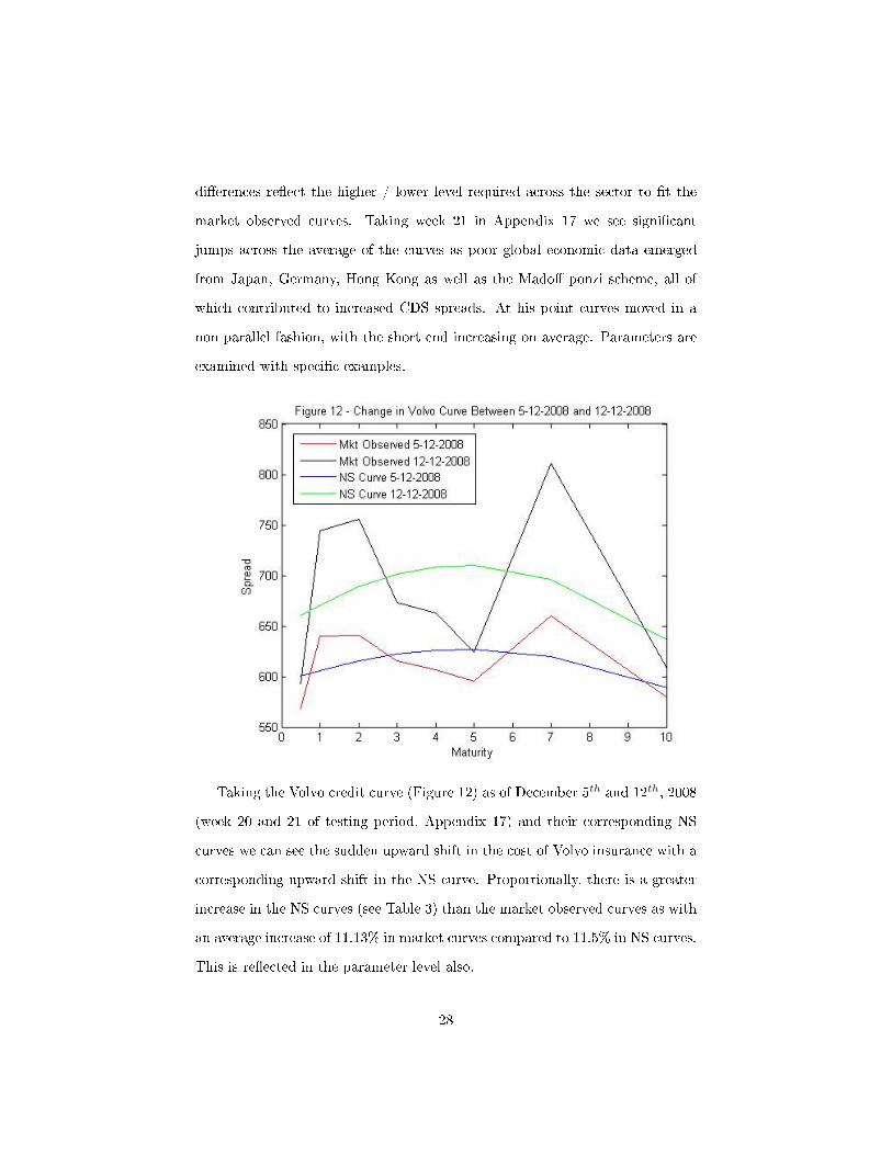
Taking the Volvo credit curve (Figure 12) as of December 5th and 12th, 2008

(week 20 and 21 of testing period, Appendix 17) and their corresponding NS

curves we can see the sudden upward shift in the cost of Volvo insurance with a

corresponding upward shift in the NS curve. Proportionally, there is a greater

increase in the NS curves (see Table 3) than the market observed curves as with

an average increase of 11.13% in market curves compared to 11.5% in NS curves.

This is re�ected in the parameter level also.

28

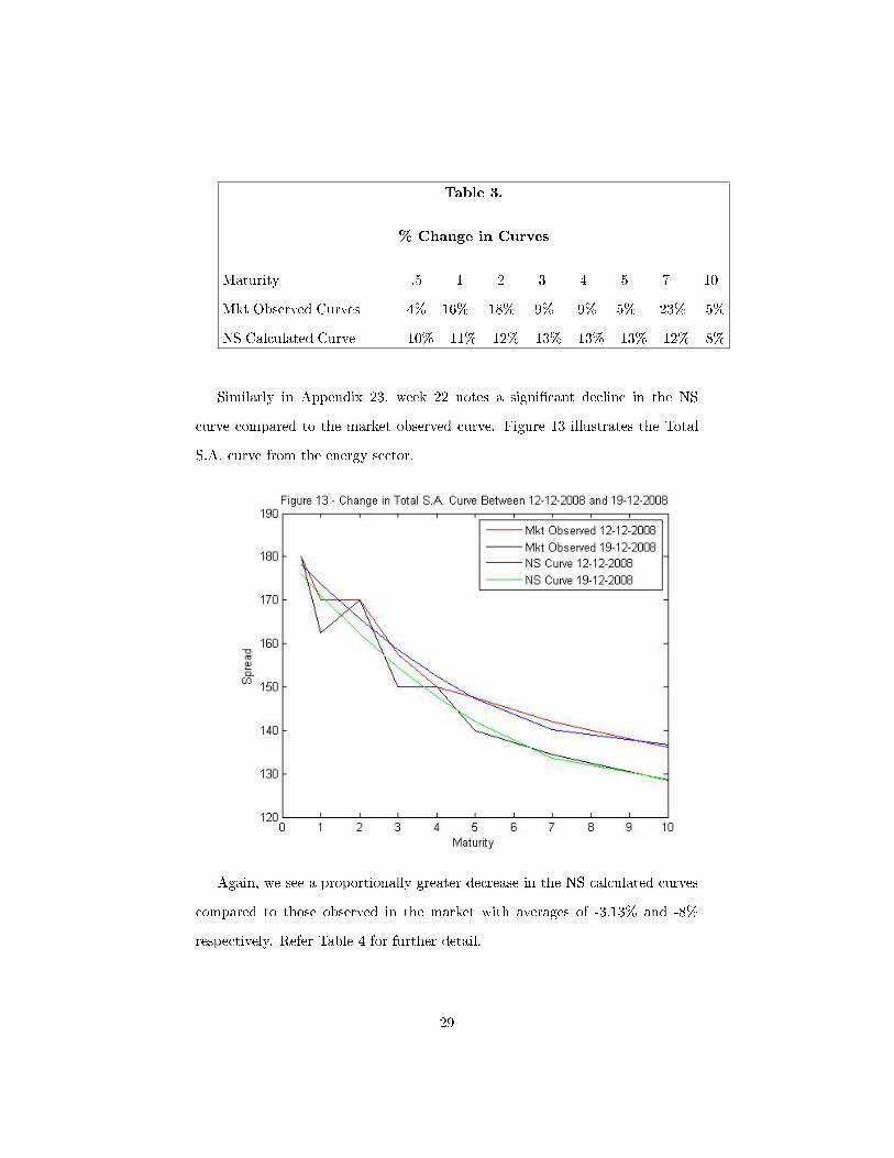
Table 3.

% Change in Curves

Maturity .5 1 2 3 4 5 7 10

Mkt Observed Curves 4% 16% 18% 9% 9% 5% 23% 5%

NS Calculated Curve 10% 11% 12% 13% 13% 13% 12% 8%

Similarly in Appendix 23, week 22 notes a signi�cant decline in the NS

curve compared to the market observed curve. Figure 13 illustrates the Total

S.A. curve from the energy sector.

Again, we see a proportionally greater decrease in the NS calculated curves

compared to those observed in the market with averages of -3.13% and -8%

respectively. Refer Table 4 for further detail.

29

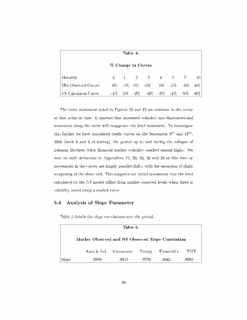
Table 4.

% Change in Curves

Maturity .5 1 2 3 4 5 7 10

Mkt Observed Curves 0% -4% 0% -5% 0% -5% -5% -6%

NS Calculated Curve -1% -2% -2% -3% -3% -4% -5% -6%

The curve movement noted in Figures 12 and 13 are common in the sector

at that point in time. It appears that increased volatility and disproportional

movement along the curve will exaggerate the level movement. To investigate

this further we have considered credit curves on the September 8th and 15th,

2008 (week 8 and 9 of testing), the period up to and during the collapse of

Lehman Brothers when �nancial market volatility reached annual highs. We

note no such deviations in Appendices 17, 20, 23, 26 and 29 at this time as

movements in the curves are largely parallel shifts, with the exception of slight

steepening at the short end. This supports our initial assessment that the level

calculated by the NS model di�ers from market observed levels when there is

volatility noted along a market curve.

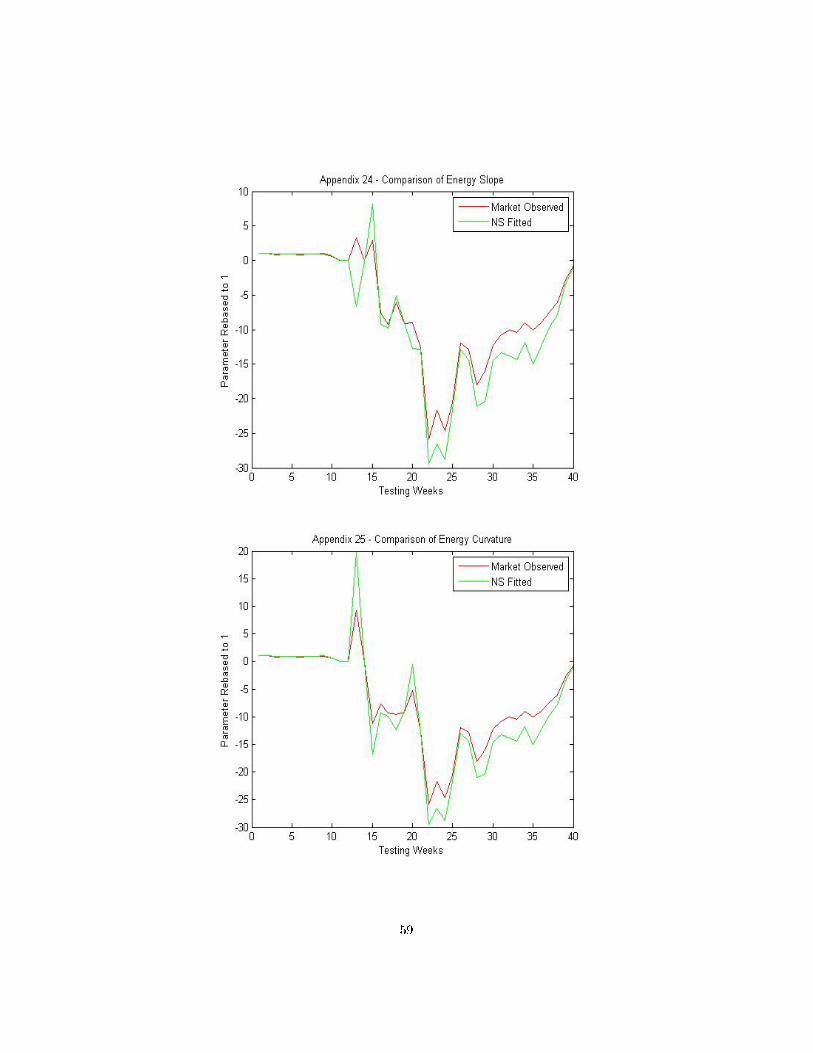
5.4 Analysis of Slope Parameter

Table 5 details the slope correlations over the period.

Table 5.

Market Observed and NS Observed Slope Correlation

Auto & Ind Consumers Energy Financial s TMT

Slope .9808 .9915 .9733 .9045 .9985

30

We note that �nancials record the lowest of all the slope parameter correla-

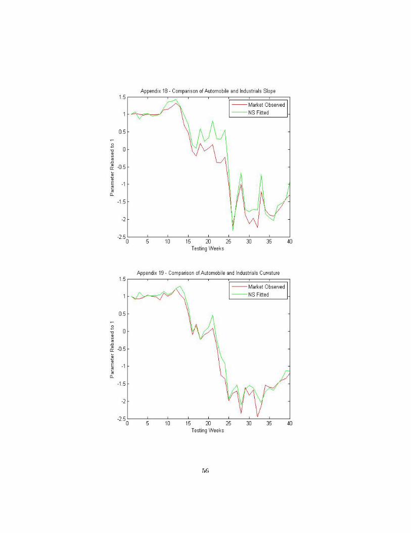
tions. These were amongst the most volatile stocks during the period. Appen-

dices 18, 21, 24, 27 and 30 graphically illustrate the slope time series for each of

the sectors over the forty week period. Here we see examples of a NS slope pa-

rameter being greater than and less than the market observed slope parameter

meaning the NS model has produced a curve with a steeper or shallower slope

than the market.

Appendix 18 notes a large shift in slope parameter between weeks 24 and

25. Figure 14 represents the Daimler curve for week 24 and 25 of the testing

period and shows a steeper sloping NS curve as of January 2nd, 2009. This

higher value is brought about from a steeper sloping longer end of the January

2nd, 2009 curve. Again, it appears the non-parallel shift in the curve is the

reason the NS slope parameter has not moved in proportion to the market slope

parameter with the steeper curve producing a higher slope value.

31

Similarly we can see a NS slope parameter that is substantially below the

market level from week 13 in Appendix 24. Upon inspection a �attening of the

energy sector curves brings the corresponding slope value down. Figure 15 shoes

the United Utilities curve for week 12 and week 13 of the testing period. Again,

this is a common theme amongst the energy curves for the period.

In both these curves a non parallel shift takes place. Again, we believe

this type of movement causes a distortion in the parameters. Upon analysis of

week 13 and 14 in Appendix 21, where there is almost zero di�erence between

parameters we �nd the average movement is a parallel shift creating proportional

slope parameter movement.

5.5 Analysis of Curvature Parameter

Appendices 19, 22, 25, 28 and 31 illustrate the curvature parameter time

line over the forty week period with Table 6 detailing the correlations.

32

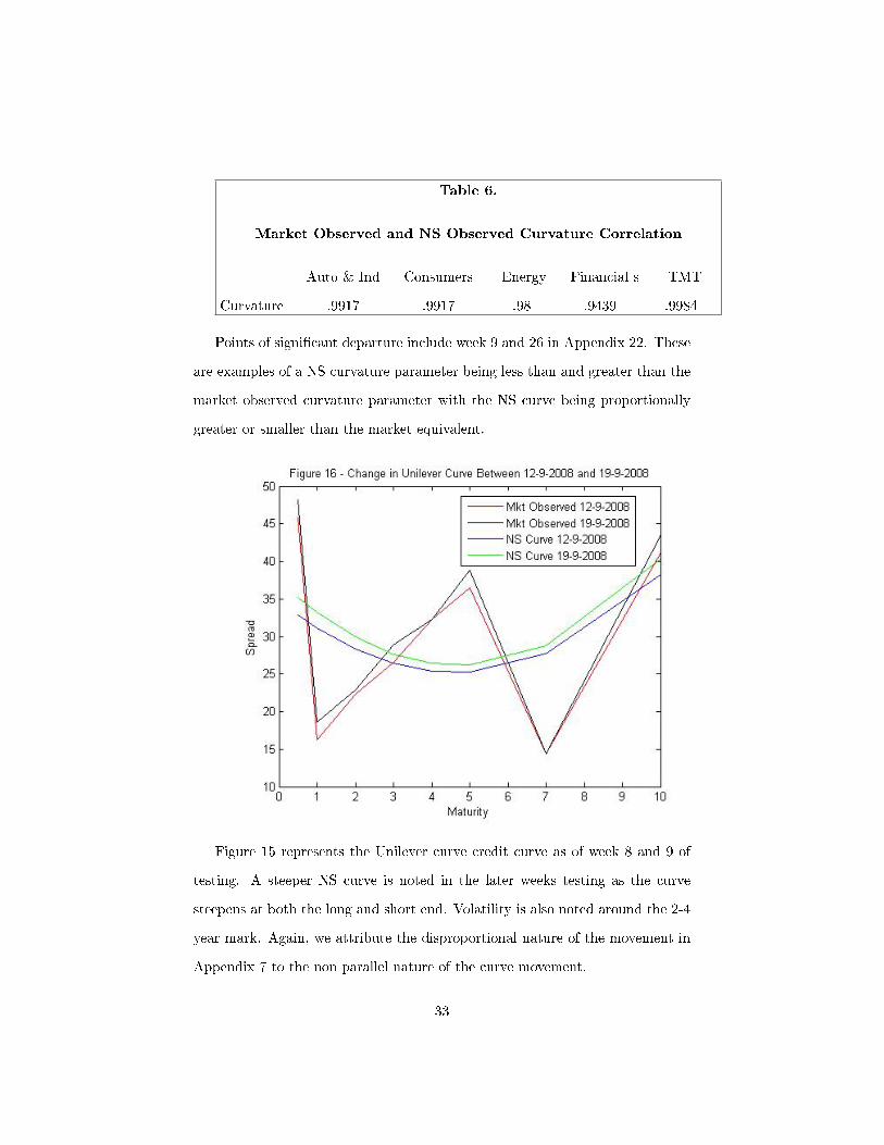
Table 6.

Market Observed and NS Observed Curvature Correlation

Auto & Ind Consumers Energy Financial s TMT

Curvature .9917 .9917 .98 .9439 .9984

Points of signi�cant departure include week 9 and 26 in Appendix 22. These

are examples of a NS curvature parameter being less than and greater than the

market observed curvature parameter with the NS curve being proportionally

greater or smaller than the market equivalent.

Figure 15 represents the Unilever curve credit curve as of week 8 and 9 of

testing. A steeper NS curve is noted in the later weeks testing as the curve

steepens at both the long and short end. Volatility is also noted around the 2-4

year mark. Again, we attribute the disproportional nature of the movement in

Appendix 7 to the non parallel nature of the curve movement.

33

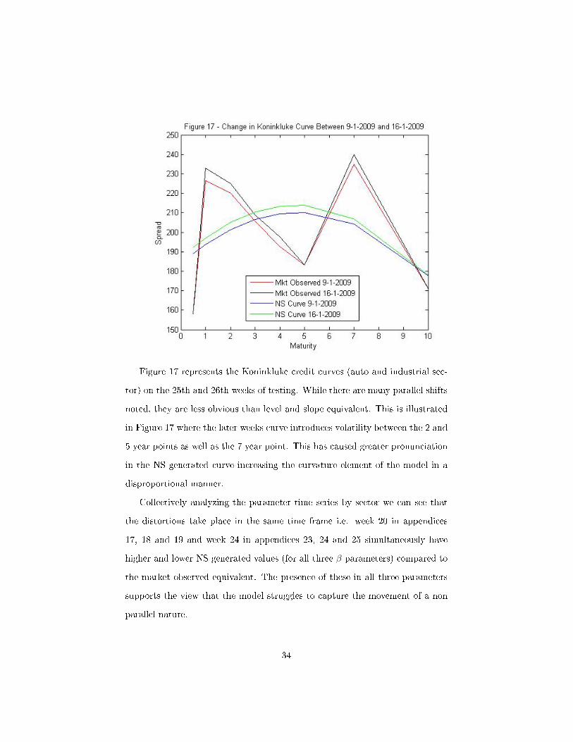
Figure 17 represents the Koninkluke credit curves (auto and industrial sec-

tor) on the 25th and 26th weeks of testing. While there are many parallel shifts

noted, they are less obvious than level and slope equivalent. This is illustrated

in Figure 17 where the later weeks curve introduces volatility between the 2 and

5 year points as well as the 7 year point. This has caused greater pronunciation

in the NS generated curve increasing the curvature element of the model in a

disproportional manner.

Collectively analyzing the parameter time series by sector we can see that

the distortions take place in the same time frame i.e. week 20 in appendices

17, 18 and 19 and week 24 in appendices 23, 24 and 25 simultaneously have

higher and lower NS generated values (for all three β parameters) compared to

the market observed equivalent. The presence of these in all three parameters

supports the view that the model struggles to capture the movement of a non

parallel nature.

34

5.6 Parameter Correlation Analysis

Table 7 illustrates how sectors noted largely positive level correlations through-

out the period with credit as an asset class performing poorly and all CDS rates

increasing over the period.

Table 7.

CDS Curve Level

Autos & Ind Consumers Energy Financial TMT

Autos & Ind 1 .739 .654 .69 .821

Consumers .739 1 .906 .356 .94

Energy .654 .906 1 .138 .77

Financial .69 .356 .135 1 .58

TMT .82 .94 .77 .58 1

A less strong set of correlations is noted in Table 8 as steepening and �at-

tening of the credit curves occurs in a less uniform fashion.

Table 8.

CDS Curve Slope

Autos & Ind Consumers Energy Financials TMT

Autos & Ind 1 .62 .489 .585 .744

Consumers .62 1 .825 .194 .928

Energy .489 .825 1 .039 .731

Financial s .585 .194 .039 1 .395

TMT .744 .928 .731 .395 1

35

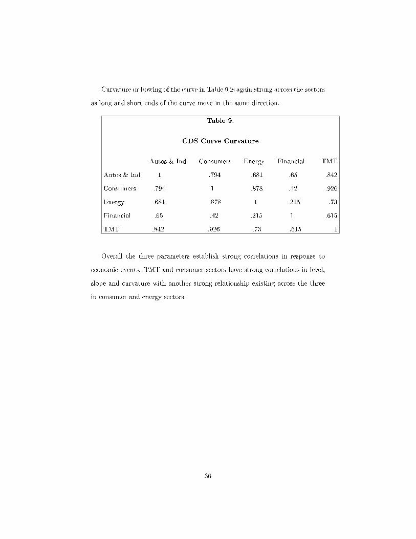
Curvature or bowing of the curve in Table 9 is again strong across the sectors

as long and short ends of the curve move in the same direction.

Table 9.

CDS Curve Curvature

Autos & Ind Consumers Energy Financial TMT

Autos & Ind 1 .794 .681 .65 .842

Consumers .794 1 .878 .42 .926

Energy .681 .878 1 .215 .73

Financial .65 .42 .215 1 .615

TMT .842 .926 .73 .615 1

Overall the three parameters establish strong correlations in response to

economic events. TMT and consumer sectors have strong correlations in level,

slope and curvature with another strong relationship existing across the three

in consumer and energy sectors.

36

6 Economic Interpretation

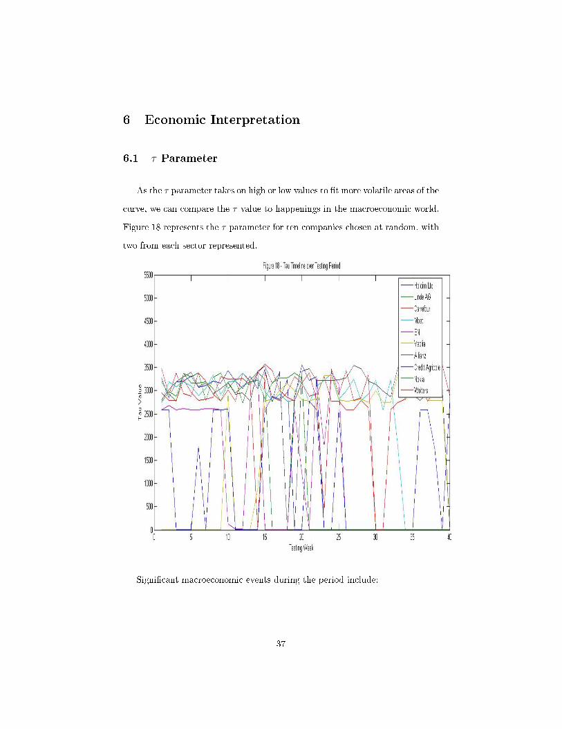
6.1 τ Parameter

As the τ parameter takes on high or low values to �t more volatile areas of the

curve, we can compare the τ value to happenings in the macroeconomic world.

Figure 18 represents the τ parameter for ten companies chosen at random, with

two from each sector represented.

Signi�cant macroeconomic events during the period include:

37

1. The �ling for bankruptcy by Lehman Brothers on September 15th, 2008

(week 10 of testing) as a results of the credit crisis.

2. The Russian �nancial crisis of November 2008 which saw $1 trillion wiped

o� the value of Russian shares (November 12th, 2008 or week 18) as a result

of plummeting oil prices (70% decline in three months), highlighting the

Russian economies dependency on the commodity.

Figure 18 notes a concentration of τ values in the greater than 2,500 level. We

note from section 5.1 that there are two potential reasons for the high τ values

(between 3,000 and 3,500), either no hump / trough or more than one hump /

trough. From data inspection we can see the market observed curves take on

one of these two forms. The increased volatility in �nancial markets at this time

introduced a second hump / trough into many curves as the short end spiked.

We interpret the lower τ values as the generation of NS curves that �t the short

end of the curve better because there is increased volatility or curvature relative

to the longer end. From 5.1 we already know that in times of macroeconomic

events and volatility at the short end of the curve, τ values will be smaller.

Immediately following the occurrence of events in week 10 and week 18 we note

an increased number of deviations from the consistently high τ values to low

values suggesting the τ value (and NS model) captures the response to the

macroeconomic event.

Strong relationships exists between all three parameters in section 5.5. This

appears reasonable as credit as an asset class noted huge losses throughout

the forty week period. Financials noted the lowest correlations as signi�cantly

more volatility was noted stemming from stimulus packages and uncertainty in

markets over individual exposures to Lehman Brothers assets. This may prove

useful for application to statistical arbitrage or hedging if relationship exits over

38

a longer period of time.

39

7 Conclusion

7.1 Main Findings

The purpose of this paper is to investigate the ability of the Nelson Siegel

model to capture the movement in the term structure of credit default swaps

over a forty week period, from July 18th, 2008 to April 17th, 2009. The main

�ndings are as follows:

1. Upon analysis of the individual curve residuals (Figures 8 and 9) it is

clear the best �tting curves are the energy sector. These are all monoton-

ically increasing with a mild hump. Other sector curves display far more

volatility and the model struggles to �t these curves with the same degree

of accuracy.

2. We note in section 5.1 that the presence of no hump / trough and more

than one hump / trough is too complicated to be described in full by the

model. This represents the majority of curves and is consistent with De

Pooter (2007) �ndings that the τ variable cannot handle the complete set

of shapes the curve takes over longer periods of time.

3. Multicollinearity contributes to the di�culty in estimating τ .

4. While there are strong correlations between the model and market pa-

rameters over time, a signi�cant number of over / under scoring of the

parameters exist. These are observed to occur at the same points in each

of the three parameters estimation as a result of non parallel shifts or

volatility in the curve sectors.

5. While the values of τ are largely in the top / bottom 15% of the 3,650

40

range, a change in its value does not distort the NS term structure signif-

icantly. Given instances where the shape of the curve is known over the

testing period, the τ value can be �xed so it produces a hump / trough at

a given point.

6. Low values of τ correspond to high volatility at the short end of the credit

curve as is seen when compared to macroeconomic events.

7. Parameter correlations between TMT and consumer sectors along with

energy and consumer sectors are extremely high in all three parameters.

7.2 Further Research

The main area of development of this paper would be to predict CDS prices

from the parameters analyzed here as done by Nelson and Siegel with interest

rate term structures. We would advise the following before undertaking this

work:

1. The NS paper uses 30 di�erent maturities while there are eight noted in the

CDS term structure. Interpolation of these eight points and a smoother

curve, would remove a lot of the volatility noted and may facilitate the

modeling of the term structure.

2. Many of the term structures note a second hump / trough. The NS model

by itself struggles to model this volatility. The introduction of the Svens-

son adjustment allows for the modeling of a second hump / trough feature

may produce τ values with greater variability than the upper and lower

15% bounds of the range.

41

3. Annaert et al advocate the use of ridge regression to address the multi-

collinearity issue.

4. While NS and Diebold and Li both refer to predicting interest rate term

structures in their papers, there is little detail on how to do it. One way we

considered undertaking this is to create a time series of the parameters, as

done in Appendices 2 - 16, and make a prediction of each of the parameters.

These predictions can be easily slotted into equation (2) and a forward

value solved for. MatLab econometrics toolbox has various functions to

predict time series such as vgxpred and vgxsim.

7.3 Concluding Remarks

While sectors note strong parameter correlations, the departures of NS

curves from market observed curves are signi�cant and frequent re�ecting the

volatility in the credit market and the models inability to deal with non parallel

shift in the credit curve. This is consistent with De Pooter (2007) observations.

Based on the work performed in this paper, it appears the volatility in the CDS

curves cannot be modeled by the NS model for the period selected. However,

should the measures outlined in section 7.2 be adopted, we believe far superior

results could be achieved.

42

8 Appendices

Appendix 1

Auto and Industrial Companies:

1. Adecco

2. Volvo

3. Akzo Nobel

4. Alstom

5. Anglo American

6. BAE Systems

7. BASF

8. Bayer AG

9. BMW

10. Cie De Saint

11. Compagnie Finc Mich

12. Daimler

13. Deutsche Post

14. European Aeroc Defe

15. Finmeccanica S.P.A.

16. Glencore Intl

17. Holcim Ltd

18. Koninklijke DSM

19. Lanxess AG

20. Linde AG

21. Rentokil AG

22. Rolls-Royce

23. Sano� - Aventis

24. Siemens AG

43

25. Solvay

26. TNT N.V.

27. Vinci

28. Volkswagen

29. Xstrata

Consumer Companies:

1. Abet Electrolux

2. British American Tobacco

3. Cadbury Schweppes

4. Carrefour

5. Casino Guipchn

6. Compass Group

7. Diageo Plc

8. Experian Finance

9. Groupe Auchan

10. Henkel KGA Aktien

11. Imperial Tobacco

12. JTI Finance

13. King�sher Plc

14. Koninklijke Ahold

15. Moet Hennessy

16. Marks and Spencer

17. Metro AG

18. Nestle A.G.

19. Next Plc

20. PPR

21. Safeway Limited

44

22. Suedzucker AG

23. Svenska Cell Abet

24. Swedish Match

25. Tate & Lyle

26. Tesco

27. Unilever

Energy Companies

1. BP

2. Centrica

3. E.ON

4. Edison S.P.A

5. EDP

6. Electricite de Fr

7. ENBW

8. ENEL S.P.A.

9. ENI S.P.A.

10. Fortum EYJ

11. Gas Natural SDG

12. Iberdrola S.A.

13. National Grid Plc

14. Reypsol YPF

15. RWE AG

16. Total SA

17. United Utilities Plc

18. Vattenfall AB

19. Veolia Enviornment

45

Financial Companies

1. Aegon

2. Allianz

3. Assic Geni

4. Aviva Plc

5. AXA

6. Banca MDP di Siena

7. Banco PPO Soco Sub

8. Banco Santander

9. Barclays Bank

10. BNP Paribas

11. Commerzbank

12. Credit Agricole AG

13. Credit Suisse

14. Deutsche Bank AG

15. Hannover Ruck

16. Intesa Sanpaolo

17. Lloyds TSB

18. Muenchener Rueck AG

19. Societe Generale

20. Swiss Reinsurance

21. Bank of Scotland

22. UBS AG

23. Zurich Insurance

Technology, Media and Telecommunications (TMT)

1. Bertelsmann AG

2. BT

46

3. Deutsche Telekom AG

4. France Telecom

5. Koninklijke KPN

6. Nokia OYJ

7. Pearson Plc

8. PT Telecom SGPS

9. Publicis Groupe

10. Reid Elsevier

11. Stimicroelectronics

12. Telecom Italia

13. Telefonica S.A.

14. Telekom Austria

15. Telenor ASA

16. Vivendi

17. Vodafone

18. Wolters Kluwer N.V.

19. WPP 2005

47

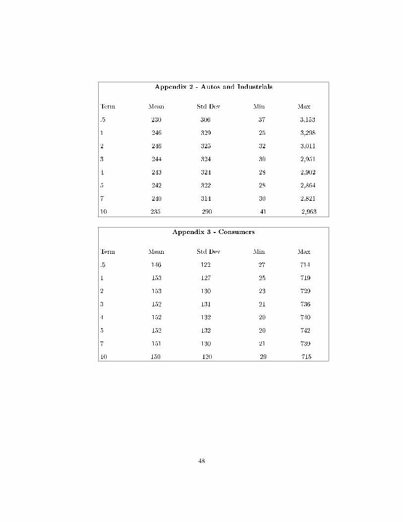
Appendix 2 - Autos and Industrials

Term Mean Std Dev Min Max

.5 230 306 37 3,153

1 246 329 25 3,298

2 246 325 32 3,011

3 244 324 30 2,951

4 243 324 28 2,902

5 242 322 28 2,864

7 240 314 30 2,821

10 235 290 41 2,963

Appendix 3 - Consumers

Term Mean Std Dev Min Max

.5 146 122 27 714

1 153 127 25 719

2 153 130 23 729

3 152 131 21 736

4 152 132 20 740

5 152 132 20 742

7 151 130 21 739

10 150 120 29 715

48

Appendix 4 - Energy

Term Mean Std Dev Min Max

.5 122 120 10 726

1 124 117 14 712

2 124 110 21 685

3 122 104 26 661

4 120 99 30 640

5 118 95 32 621

7 115 88 35 601

10 111 83 38 598

Appendix 5 - Financials

Term Mean Std Dev Min Max

.5 142 109 37 880

1 142 110 35 892

2 140 110 33 911

3 140 109 31 924

4 140 109 30 930

5 140 108 30 931

7 140 106 33 913

10 142 102 34 839

49

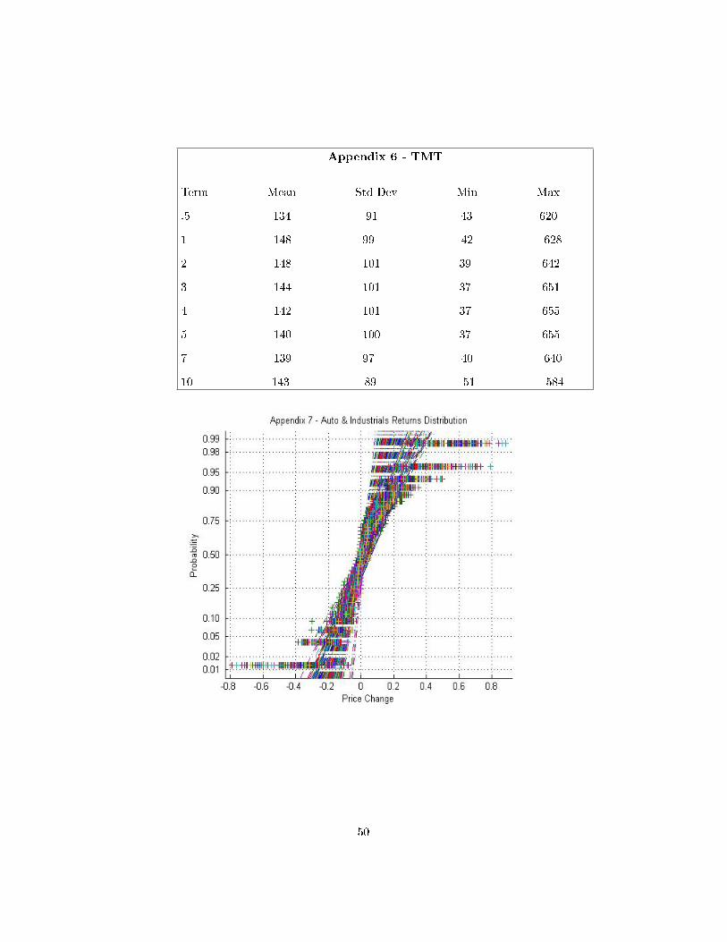
Appendix 6 - TMT

Term Mean Std Dev Min Max

.5 134 91 43 620

1 148 99 42 628

2 148 101 39 642

3 144 101 37 651

4 142 101 37 655

5 140 100 37 655

7 139 97 40 640

10 143 89 51 584

50

51

52

53

54

55

56

57

58

59

60

61

62

9 Bibliography

1. Durand, D. (1942), �Basic Yields of Corporate Bonds�, National Bureau

of Economic Research, June 1942, pp 8-9.

2. Friedman, M. (1977), �Time Perspective in Demand for Money�, Scan-

dinavian Journal of Economics, Wiley Blackwell, Vol 79 (4), pp. 397 -

416.

3. Nelson, C. and Siegel, A. (1987), �Parsimonious Modelling of Yield Curves�,

The Journal of Business, Vol. 60, Oct, 1987, pp.473-489.

4. Bank for International Settlements.�Zero-Coupon Yield Curves : Techni-

cal Documentation�, Bank for International Settlements, BIS Paper No.

25, 2005.

5. Wood, J (1983). �Do yield curves normally slope up? The term struc-

ture of interest rates, 1862-1982�. Economic Perspectives, Federal Reserve

Bank of Chicago, July/August, 1983: pp. 17-23.

6. Filipovic, D. (1999), �A Note on the Nelson-Siegel Family�, Damir Fil-

ipovic, [online] Available at<http://www.vif.ac.at/�lipovic/PAPERS/Nelson-

Siegel.pdf> [Accessed 14th June 2011].

7. Hurn, A.S., K.A. Lindsay, and V. Pavlov. (2005),�Smooth Estimation of

Yield Curves by Laguerre Function�, Queensland University of Technology

Working Paper, 2005, pp. 1042 - 1048.

8. De Pooter, M, �Examining the Nelson-Siegel Class of Term Structure

Models: In-Sample Fit versus Out-of-Sample Forecasting Performance�

(September 23, 2007). Available at SSRN: http://ssrn.com/abstract=992748

[Accessed 30th June 2011].

63

9. Diebold, F.X. and Li, C. (2006), �Forecasting the Term Structure of Gov-

ernment Bond Yields�, Journal of Econometrics, 130, pp. 337-364.

10. Annaert, J., Claes, A.G.P., De Ceuster, M, J, K., Zhang, H. (n.d.), �Es-

timating Nelson-Siegel - A Ridge Regression Approach�, University of

Antwerp. [online] Available at <http://www.efmaefm.org/OEFMAMEETINGS/EFMA%20MEETINGS/2010-

Aarhus/EFMA2010_0387_fullpaper.pdf> [Accessed 13th July 2011].

11. Svensson, L.E.O., (1994).�Estimating and Interpreting Forward Interest

Rates:Sweden 1992 - 1994�, International Monetary Fund, WP/94/114.

12. Gauthier, G and Simonato, J, �Linearized Nelson-Siegel and Svensson

models for the estimation of spot interest rates�, HEC Montreal, [online]

Available at <http://69.175.2.130/~�nman/Reno/Papers/NelsonSiegelSvensson.pdf>

[Accessed 27th June 2011].

13. Litterman, R. and J. Scheinkman, �Common Factors A�ecting Bond Re-

turns�, Journal of Fixed Income, Vol 1, No 1 (June 1991), pp. 54-61.

14. Dullmann, K. and Uhrig-Homburg, M. �Pro�ting Risk Structure of Inter-

est Rates:An Empirical Analysis for Deutschemark-Denominated Bonds�,

European Financial Management, Vol. 6, No. 3 (2000), pp. 367-388.

15. Martellini, L, and Meyfredi, J. C., �A Copula Approach to Value-at-Risk

Estimation for Fixed-Income Portfolios�, Journal of Fixed Income, Vol.

17, No. 1 (June 2007), pp. 5-15.

16. Fabozzi, F.J., Martellini, L. And Priaulet, P., �Predictability in the Shape

of the Term Structure of Interest Rates with Smoothing Splines�, Finance

and Economics Discussion Series - Federal Reserve Board, September,

1994.

64

17. Cairns, A.I.G., and Pritchard,�Stability of Descriptive Models for the

Term Structure of Interest Rates with Applications to German Market

Data�, Brotosh Actuarial Journal, Vol. 7(2001), pp. 467 - 507.

18. Hull, J.C. and White, A, �Valuing Credit Default Swaps I: No Coun-

terparty Default Risk�, NYU, Working Paper No. FIN-00-021. (April

2000), Available at SSRN: http://ssrn.com/abstract=1295226 [Accessed

27th June 2011].

65