A Unified Resource-Constrained Framework for Graph SLAM

Liam Paull, Guoquan Huang, and John J. Leonard

Abstract— Graphical methods have proven an extremelyuseful tool employed by the mobile robotics community to frameestimation problems. Incremental solvers are able to processincoming sensor data and produce maximum a posteriori(MAP) estimates in realtime by exploiting the natural sparsitywithin the graph for reasonable-sized problems. However, toenable truly longterm operation in prior unknown environ-ments requires algorithms whose computation, memory, andbandwidth (in the case of distributed systems) requirementsscale constantly with time and environment size. Some recentapproaches have addressed this problem through a two-stepprocess - first the variables selected for removal are marginal-ized which induces density, and then the result is sparsified tomaintain computational efficiency. Previous literature generallyaddresses only one of these two components.

In this work, we attempt to explicitly connect all of theaforementioned resource constraint requirements by consider-ing the node removal and sparsification pipeline in its entirety.We formulate the node selection problem as a minimizationproblem over the penalty to be paid in the resulting sparsifi-cation. As a result, we produce node subset selection strategiesthat are optimal in terms of minimizing the impact, in termsof Kullback-Liebler divergence (KLD), of approximating thedense distribution by a sparse one. We then show that oneinstantiation of this problem yields a computationally tractableformulation. Finally, we evaluate the method on standarddatasets and show that the KLD is minimized as comparedto other commonly-used heuristic node selection techniques.

I. INTRODUCTION

In many realistic application scenarios, robots are requiredto navigate over long time periods in unknown and uncertainenvironments by performing simultaneous localization andmapping (SLAM). For example, a team of autonomousunderwater vehicles (AUVs) is often used to cooperativelycollect data in the ocean (e.g., for seabed mapping). Re-cently, graph-based approaches have emerged as one of themost popular approaches to SLAM [1]. In this formulation,each new sensor measurement adds a new edge (constraint)between two nodes (states) into the graph. The most likelyconfiguration of the states can be efficiently found by exploit-ing the sparse structure of the system, and an incrementalmethod (e.g. [2]) can be further utilized in order to achievereal-time performance for “medium-sized” problems.

This work was partially supported by the Office of Naval Research undergrants N00014-10-1-0936, N00014-11-1-0688 and N00014-13-1-0588 andby the National Science Foundation under grant IIS-1318392, which wegratefully acknowledge.

L. Paull and J. Leonard are with the Computer Science and ArtificialIntelligence Laboratory (CSAIL), MIT, Cambridge, MA 02139, USA.Email: {lpaull,jleonard}@mit.edu

G. Huang is with the Dept. of Mechanical Engineering, University ofDelaware, Newark, DE 19716, USA. Email: ghuang@udel.edu

*The authors would like to thank Mladen Mazuran for helpful discussionsduring the preparation of the manuscript

Fig. 1: In the absence of node reduction strategies, the size of theSLAM graph will grow without bound. Top: The Manhattan 3500dataset [3] with 3500 poses in SE(2) and 5599 constraints. Theblue edges denote the entire dataset and the red circles are 500poses that have been subselected. Bottom Left: The removal ofthe 3000 poses induces density in the graph. Here we show thesparsity structure of the resulting information information matrix.Bottom Right: In order to maintain computational efficiency,the dense representation is approximated by a sparse one. In thiswork we propose to choose the nodes to remove so that the sparserepresentation is as close as possible (in the KL divergence sense)to the dense one.

Notwithstanding the efficiency of these graph-SLAM ap-proaches, they are not directly applicable to large-scaleproblems because resources such as memory, computation,and communication in multi-robot systems do not scaleworse than constantly. For example, communication band-width through acoustics available to AUVs is typically verylimited [4]. As a result, without removing states from thesystem, these graph-based methods will lead to resourceconstraint violation as mission duration and operational areaincrease.

To address this issue, recent work has focused eitheron how to select which nodes to remove, or on how tomaintain sparse connectivity between nodes, but rarely both.In particular, marginalization is often used to remove nodes,which is achieved through Schur complement on the Hessian(information) matrix. Note that marginalization enforces a“node constraint” on the total number of variables. How-

ever, this process induces density and significantly increasesthe overhead of communication bandwidth or computationcomplexity, which in effect motivates edge sparsification [5],[6], [7]. Specifically, a Kullback-Liebler divergence (KLD)minimization is formulated to find a sparse informationmatrix to approximate the original dense one. Note that spar-sification allows us to satisfy an “edge constraint” or “densityconstraint”, for example, for computational efficiency and/orbandwidth considerations. However, this process is approxi-mate and the penalty that we pay can be quantified in termsof KLD between the dense true distribution and its sparseapproximation.

For a given application, a problem-specific approach toselect and remove nodes may exist. For instance, one recentwork proposed removing the nodes at which there is aminimum probability of collision with the environment fora navigation objective [8]. However, we argue that in theabsence of problem-specific node selection strategies (i.e.,every node is an equal candidate for removal), the optimalchoice of nodes to remove through marginalization in orderto satisfy node number constraints are the ones that will incurthe minimum penalty in the subsequent sparsification to meetthe edge constraints.

These two operations, marginalization and sparsification,are usually treated as distinct. The algorithms of noderemoval via marginalization do not consider the attainableperformance of the subsequent sparsification, and conversely,the sparsification approaches are agnostic to the node se-lection used to choose which nodes to marginalize. Inthis work, we tightly couple these two processes into asingle unified optimization framework, whose objective isto minimize the information loss due to graph reductionwhile being constrained by limited resources available. Inparticular, our proposed unified framework aims to optimallyaccount for the resource constraints of computation, memory,and communication bandwidth. To prove this concept, afterformulating the problem in the general sense, we provideone tractable solution instance. To validate this solution, wecompare against the node selection strategies available inthe literature and show that in our case the constraints aremet with less penalty in terms of KLD between the densedistribution and the sparse approximation.

II. RELATED WORK

Graph reduction algorithms can be categorized into twoclasses: (i) selecting which measurements and/or variables todiscard, and (ii) marginalizing variables and then sparsifyingmeasurements. In what follows, we briefly review these twoclusters of literature.

A. Measurement/variable selection

1) Measurement selection: The basic idea of most mea-surement selection approaches is to evaluate the relative “in-formativeness” of measurements themselves and then discardthe least useful. In particular, Kretzschmar et al. [9] intro-duced pose-graph compression for laser-based SLAM, inwhich nodes are selected for removal based on the amount of

new information provided by their respective laser scans. Theless informative scans are removed and then the associatedposes are marginalized followed by a Chow-Liu tree (CLT)-based [10] approximation to regain sparsity. Similarly, Ilaet al. [11] provided a relative information metric to evaluatewhether edges should even be added to the pose graph in thefirst place, as well as to remove uninformative loop closureconstraints.

2) Variable selection: The question of how to selecta subset of variables to better support localization and/ormapping operation has been investigated. In [12], a Euclideandistance criterion is employed for node removal to ensurethat the size of the state vector grows only with the size ofthe mapped environment. However, this approach does notbound the number of measurements. Similarly, downsam-pling features based on a visual-saliency measure in vision-based navigation systems has also been explored in order toimprove loop closing [13], [14], [15]. In appearance-basedvisual SLAM approaches a similar problem is framed as“dictionary learning” where the size of the dictionary mustbe reduced. For example, in a online “sparsity-cognizant”approach to dictionary learning was proposed by Latif et.al. [16]. Other work considers variable selection to supportthe objective of navigation. For example, Strasdat et al.[17] introduced a reinforcement learning based landmarkselection policy to minimize the robot position error at thegoal. Lerner et al. [18] considered single camera framebased landmark selection in terms of a “severity function.”And Sala et al. [19] chose the minimal set of landmarksthat are viewable from every point in the configurationspace. Moreover, Mu et al. [8] recently proposed a singleframework for both landmark and measurement selectionto support navigation. Other landmark and measurementselection techniques are also available but task-specific, e.g.,uniform landmark selection [20] and entropy-based landmarkselection [21] for the localization and mapping objective,as well as an incremental approach [22]. By contrast, inthis work, we address the variable selection strategy byexplicitly considering the resource constraints to be satisfiedand choose the variables whose subsequent removal (throughmarginalization and sparsification) will incur the least infor-mation loss.

B. Node marginalization and edge sparsfication

Since marginalization induces dense connectivity acrossthe Markov blanket of the marginalized node, recent researchefforts have been devoted to further reduce the edges of thegraph. In particular, Vial et al. [23] are among the first to for-mulate this sparsification problem as a convex optimizationthat minimizes the KLD between the dense distribution andits sparse approximation. In our prior work [5], we furtherregularize this formulation with `1-norm, which is appealingin its flexibility as it does not commit to any sparse graphstructure. However, one challenge with this approach is thatdirect control over the structure of the resulting sparsifiedinformation matrix is lost. To mitigate this issue, Carlevarisand Eustice [24] introduced generic linear constraints (GLCs)

to approximate the dense factors induced by marginalizationbased on the CLT approximation. Most recently, Mazuranet al. [7], [25] improve the previous results by allowingnonlinear measurements to approximate the dense factorswith “virtual” measurements which can be defined arbitrarilyand then insightfully formulating the convex optimizationover the measurement, rather than state, information matrixand proving that it remains convex. However, designing thesevirtual measurements is nontrivial and task specific.

It is important to note that none of these approachesprovides any insight into how nodes should be selectedto be marginalized, although this choice of nodes has asignificant impact on the optimal KLD that is attainablein the sparsification stage. Moreover, they do not explicitlyconsider constraints other than computation, which clearlyis not adequate for real robotic systems since other keyresource constraints such as memory and communicationcannot be ignored. In our recent work [4], communicationconstraints were taken into account in building multi-AUVSLAM systems. Specifically, marginalization is performedover the robot poses so that only maps are communicatedto save communication throughput, and then the dense mapconnectivity is sparsified using a convex optimization similarto [7]. In this work, building upon our prior work [5], [4],we propose a unified framework to incorporate both edge(bandwidth or computation) and node (memory) constraints.

III. PROBLEM FORMULATION

Let X = [xT1 , · · · ,xTN ]T be the set of states (robot posesand/or landmark positions) that we seek to estimate, andZ = [zT1 , · · · , zTM ]T be the set of conditionally independentmeasurements. By assuming that p(zj |X) = p(zj |Xj), i.e.,Xj is the subset of states that are constrained by measurementzj , we can write the measurement model as follows:

zj = hj(Xj) + ηj , ηj ∼ N (0, D−1j ) (1)

where we assume additive white Gaussian noise.In graph SLAM, we aim to to find the most likely

configuration of the states X given the measurements that wehave made (i.e., maximum likelihood estimation or MLE).This problem can be shown to be equivalent to the followingnonlinear least-squares (NLS) problem [1]:

X̂ = argminX

M∑j=1

||zj − hj(Xj)||2D−1j

(2)

where ||e||Σ denotes the Mahalanobis distance (energy norm)and Dj ∈ R|zj |×|zj | is the measurement noise informationmatrix. To solve (2), due to the nonlinearity of measurementmodel (1), an iterative algorithm such as Gauss-Newton isoften employed. Specifically, starting from an initial guessX̂(0), we iteratively solve for the (locally) optimal error state(increment) which is then used to update the state estimate:

δX(k+1) = argminδX

M∑j=1

||zj−h(X̂ (k)j )−H(k)

j δX||2D−1

k

(3)

X̂(k+1) = X̂(k) + δX(k+1) (4)

whereH

(k)j =

∂h(Xj)∂X

|X=X̂(k) ∈ R|zj |×N

is the measurement Jacobian evaluated at the current stateestimate in the k-th iteration. In solving (3), an information(Hessian) matrix is typically required, which is given by:

I =

M∑j=1

HTj DjHj = HTDH

with H ,

H1

...HM

, D ,

D1 · · · 0...

. . ....

0 · · · DM

(5)

It is important to note that the sparsity pattern of Icorresponds exactly to the connectivity in the graph, i.e.,the information matrix encodes the conditional dependence:

I[i,j]

{6= 0 ∃zk|(xi,xj ∈ Xk)= 0 otherwise

(6)

Consequently, we can evaluate the number of distinct non-zeros that will appear in I without ever having to calculateit using the following iterative equation:

||I||0 =

M∑j=1

|P2(Xj)| − |P2(Xj)⋂{j−1⋃i=1

P2(Xi)}| (7)

where P2 is the subset of power set of cardinality at most 2.It is clear that the size of the NLS problem (3)-(4) grows

as new robot poses and/or landmark positions are added intothe graph. The graph will eventually become prohibitivelylarge for real-time performance, thus necessitating graphreduction.

A. Marginalization of nodes

To reduce the graph, marginalization is often used toremove nodes (i.e., reduce the size of the state space N ). Tothis end, we partition all states into two subsets: the states wewish to keep, XR, and the states we wish to remove, XM .Marginalization over the canonical parametrization of theGaussian distribution is performed via Schur complement:

Id = IRR − IRMI−1MMIMR (8)

I =

[IRR IMR

IRM IMM

](9)

where Id in general becomes more dense than the originalblock matrix IRR. For subsequent optimization, a new set ofdense factors can be generated using this dense informationmatrix Id as well as the current estimate of the removedstates X̂R [5], [24], [7].

B. Sparsification of edges

While marginalization reduces the size of the graph, itadversely increases the density of the graph. To furtherreduce the graph, one approach is to replace the densedistribution over the Markov blanket (subgraph) with a sparseapproximation, for example, using the CLT approximationwhich is the optimal minimal yet connected distribution [24].

However, this approach does not guarantee consistency (i.e.,information might be added to the graph) and the treestructure may not be desirable. Alternatively, one seeksto solve for a sparse approximation based on the convexoptimization of minimizing KLD between the original densedistribution and the new sparse one [23]:

minIs∈S++

DKL(N (X̂, I−1s )||N (X̂, I−1

d ))

= minIs∈S++

tr(IsI−1d )− ln(|Is|)

(10)

This method has the advantage that conservativeness can beenforced through the additional constraint Is � Id. However,it remains open how to select the edges to remove. Optionsinclude again to choose the CLT structure [6], to enforcesparsity through sparsity regularization [5] or use problem-specific predefined graph structure [4].

IV. RESOURCE-CONSTRAINED GRAPH SLAMIn this section, we propose a unified optimization frame-

work that seeks to find an optimal reduced graph withrespect to both nodes and edges, while meeting all resourcerequirements by explicitly expressing them as the constraintsimposed onto the pertinent optimization variables.

A. Edge constraints

The number of edges (measurements) in the graph canbe seen as directly aligning with a bandwidth constraint inthe case of multi-robot systems [4], but it also connectsto the computation required to solve for the MLE estimate[see (3) and (4)]. To derive the exact computation requiredas a function of the edge density, or fill-in, is challenging(if not impossible) since it is heavily impacted by otherfactors such as initial estimate, nonlinearity of measurementfunctions, and so on. However, in general, the efficiency ofNLS solvers largely depends on the fill-in of the informationmatrix, which impacts the efficiency of back-substitutionand covariance recovery [2]. Based on this key observation,we formulate the following reduction problem with graphdensity as the computation constraint:

Problem 1. Graph Density as Computation Constraint

minIs∈S+

DKL(N (X̂, I−1d )||N (X̂, I−1

s ))

s.t.||Is||0N

≤ κdensity(11)

where Is is the sparse information matrix, Id is the denseinformation matrix, X̂ is the most recent MAP estimate, Nis the dimensionality (number of nodes times dimension ofeach node) and κdensity is the edge density constraint.

In the case of multi-robot distributed systems, we alsoconsider the bandwidth as a finite resource. In this case, it isadvantageous to consider a variation on (10) is to formulatethe minimization over the measurement information of thenew “virtual measurements” Ds [7], which are related tothe sparse state information through Is = HT

s DsHs. Asproposed in [4] if ||Ds||0 ≤ ||Is||0, where ||Is||0 is incre-mentally calculated through (5), and the virtual measurement

functions are known to all robots (presumably agreed uponat the start) then it is advantageous to only send the non-zero values in Ds. This motivates the following bandwidth-constrained sparsification problem:

Problem 2. Edge Number as Bandwidth Constraint

minDs∈D

DKL(N (X̂, I−1d )||N (X̂, (HT

s DsHs)−1))

s.t. ||Ds||0 ≤ κbandwidth(12)

where D is the set of block diagonal positive definite matricesthat correspond to the block structure of the measurements.

It should be pointed out that the actual Jacobian matrices,Hs can be computed by the receiver, since the structure ofthe nonlinear measurements is known and the linearizationpoints, X̂R, are also sent [4]. Consequently, the sparseinformation matrix can be recovered.

B. Variable constraint

In general, the number of nodes, and thus the size of theNLS problem (2), grows without bound as robot(s) operate.Therefore, it is necessary to remove nodes to retain constant-time scalability and enable long-term operation of mobilerobots in unknown environments. To this end, we effectivelyimpose an upper bound, κnode, on the number of nodes thatcan be contained in the graph.

Problem 3. Node Number as Memory Constraint

minXR⊂X

f(XR)

s.t. ||XR||0 ≤ κnode(13)

where XR is a subset of the entire set of variables, and f(·)is an objective function that is a design choice.

The cost function f(·) may be designed based on someapplication-specific requirements. For example, it can bemutual information [9], functions of euclidean distance [12],mutual information of associated sensor data, or probabilityof collision with obstacles [8]. We propose an alternativedefinition for the function f(·) as is detailed in the followingsubsection.

C. Unified optimization with edge and variable constraints

The central idea behind this work is that in the absenceof front-end data considerations or problem-specific node re-moval strategies, the best way to choose the nodes to removeis to select the ones that will induce the least penalty inthe subsequent sparsification. Hence, we combine Problems1, 2 and 3 to formulate one unified optimization problemconstrained by both edge and variable requirements. Inparticular, by defining the objective function f(·) in Problem3 by the output of the KLD minimization of the sparsificationproblems, we get the following unified formulation:

Problem 4. Resource-Constrained Graph Reduction

minXR⊂X

{minIs∈S+

Dkl(N (X̂, I−1d )||N (X̂, I−1

s ))

s.t. ||Is||0 ≤ κdensity||Ds||0 ≤ κbandwidth

}s.t. ||XR||0 ≤ κnode

(14)

Ds and Is are related through Is = HTs DsHs, and the node

subset determines the information matrix partitioning in thecalculation of Id as given by (8).

Both of the edge constraints, κdensity and κbandwidth, andthe node constraint, κnode, are enforced in Problem 4. Theinequalities in (13) and (14) can be treated as equalities inthe case that we wish to enforce that the resources are fullyutilized.

V. SOLVING PROBLEM 4

Due to the combinatorial nature, it is in general com-putationally intractable to solve Problem 4 analytically. Tomitigate this issue, let us first turn our attention to theinner optimization which is convex, and then to the outeroptimization which is combinatorial.

A. Solving the inner convex optimization

Given a potential subset of nodes XR, one standard ap-proach for solving this problem is to enforce sparsity through`1-regularization on the information matrix. This is done byadding the term λ||Is||1 to the objective function in Problem1 and removing the constraint. The `1 norm is the closestconvex relaxation of the `0 norm but is known to promotesparsity, where the tuning parameter λ determines the levelof sparsity. This can be solved by an interior point methodor using the alternating direction method of multipliers(ADMM) [5]. While this is an appealing approach, it is stillpreclusively slow since the optimization will have to iterateto convergence for every node that is evaluated.

Instead, we adopt the formulation for sparsification viaminimizing the measurement information matrix as shownin Problem 2. In this case, we have direct control over thedesign of the Jacobian matrix Hs, and the block structure ofthe measurements, encoded in Ds that together will deter-mine the resulting sparsity. As such, we can satisfy the edgeconstraint by construction through appropriate specificationof these matrices. Moreover, it is shown in [25] that inthe case that Hs is invertible, the optimal measurementinformations are computable in closed form:

Di = ({HsI−1d HT

s }i)−1 (15)

where the {·}i selects the ith block of the inner matrix. Theresulting information matrix is given by Is = HsDsH

TS with

Ds =

D1 0 · · · 00 D2 · · · 0...

.... . .

...0 0 · · · DK

(16)

We now build the Jacobian matrix that consists of relativepose-pose or pose-landmark measurements over the CLTacross the Markov blanket of the node(s) being removed,which is guaranteed to be full rank and square (and hencenon-singular). We can then add additional edges as permittedby adding correlations between these measurements in theblock measurement information structure [25].

Although not necessarily explicitly stated, current ap-proaches such as [25] marginalize one node at a time,performing a sparsification after each one. We note here thatneither the resulting graph topology, nor the approximationare independent of the node elimination order in this case.Moreover, it is impossible to enforce hard global sparsityrestrictions this way. Instead sparsity is enforced locallyupon removal of each node. In contrast, here, after selectingthe nodes designated for removal, we eliminate them allsimultaneously. In the case where one node is inside theMarkov blanket of another (and necessarily vice-versa) thenthe Markov blankets should be merged. As a result, theresulting graph topology after marginalization and sparsifica-tion is unique and optimal (as a result of the CLT optimality)and actually can be more sparse than the resulting graph afterincremental node removal, which imposes a separate localCLT structure on each node as it is removed.

We proceed as follows. We begin by using the knowngraph topology and the candidate nodes XR to generate aset of distinct Markov blankets X{p} ⊂ XR, p = 1, · · · , P ,with 1 ≤ P ≤ |XM | where |XM | is the number of nodesto be removed times the dimension of an individual node.We perform a Schur complement to generate Id once using(8) but then decompose the result into the individual densemarginal information matrices for each Markov blanket,I{p}d . For each Markov blanket, we perform a CLT decompo-sition and generate a non-singular Jacobian H{p}s consistingof relative pose-pose or pose-landmark measurements overthe CLT evaluated at the current estimates of the nodes,X̂{p}. We subsequently solve for the block measurementinformations using (15). We can solve for the minimum KLDby computing the sparse information matrix over the Markovblanket and re-inserting it into the KLD objective function(10). Finally, the total KLD for this node combination canbe evaluated by summing the individual KLDs since theestimates of the variables in XR but not in any Markovblanket will remain constant. As a result, the function f(XR)from Problem 3 can be expressed as:

f(XR) =

P∑p=1

log det(H{p}s D{p}s (H{p}s )T )

+ tr(H{p}s D{p}s (H{p}s )T (I{p}d )−1)

(17)

where the edge constraint satisfaction is explicitly guaranteedthrough the design of the Jacobians and block structure of themeasurements. Note that we could also optionally guaranteeconsistency by efficiently projecting into the consistencyspace using an eigendecomposition of the small local infor-mation matrices [4]. The algorithm for evaluating a candidatesolution is summarized in Algorithm 1.

Algorithm 1 Solving the inner optimization in Problem 4for one candidate node subset XR

Input: XR - the set of nodes that should be retainedX̂R - the current map estimates of the nodes in XR

I - the full information matrixκdensity , κbandwidth - the edge contraints

Output: D∗KL1: I =

[IRR IMR

IRM IMM

]2: Id = IRR − IRMI−1

MMIMR

3: Extract the P separable Markov blankets X{p}, p = 1..Pbased on nodes to remove XR and connectivity encodedin I

4: D∗KL ← 05: for all p = 1, . . . , P do6: I{p}d ← block information matrix according to X{p}

7: Find minimum spanning tree (CLT) for Markov blan-ket p

8: H{p}s ← Jacobians for pairwise measurements over

spanning tree evaluated at X{p}R9: (optional) greedily add conditional dependencies to

measurements until reach κdensity or κbandwidth10: increment D∗KL by log det(H

{p}s D

{p}s (H

{p}s )T ) +

tr(H{p}s D{p}s (H

{p}s )T (I{p}d )−1)

11: end for

B. Solving the outer combinatorial optimization

We solve the combinatorial outer optimization using abranch and bound method over the partial order of nodesubsets. Fig. 2 illustrates the process, where there are 8nodes and 10 edges (unary factors don’t count as edges).The corresponding partial order is shown in Fig. 3. Each row,N , in the partial order contains all possible combinations ofN nodes. Edges in the partial order (with arrows as shown)correspond to a single node removal. We bias the search inthe tree to follow paths minimizing the “edge cost” which isdefined as follows:

Definition 1. (Edge Cost) The edge cost is the number ofedges added to the graph by removing an additional node(moving down one level in the partial order) assuming denseconnectivity over the nodes in the Markov blanket

The edge costs are labeled on the edges in the partial orderin Fig. 3. These edge costs can be calculated quickly bylooking at the sparsity pattern in the Schur complement sub-blocks, IRR and IRMI−1

MMIMR. The matrix IRR encodesthe existing connectivity over the remaining nodes. Everynon-zero component in IRMI−1

MMIMR without a counterpartin IRR denotes the addition of a new edge over the Markovblanket that did not previously exist.

One can immediately observe that these edge costs dono necessarily align with the least connected nodes, butinstead the nodes whose Markov blankets have the densestconnectivity. For example, consider removal of node X7 asshown in Fig. 2-bottom right. It is connected to nodes X6

x1 x2 x6 x7

x5x4x8 x4 x3 x5x8

x1 x6 x7

x5x4x8 x4 x3 x5x8

x1 x2 x6

x5x4x8 x4 x3 x5x8

Remove 7Remove 2

Fig. 2: Example of graph reduction. Large nodes constitute vari-ables to be estimated. Small blue circles are constraints (factors)derived from sensor measurements. Top: Original graph with eightnodes and 10 edges. Bottom Right: Node X7 removed. Sincethe nodes connected to X7 were already connected, the constraint(shown in green) can be updated resulting in no new edges. Graphnow has 7 nodes and 8 edges. Bottom Left: Node X2 is removed.3 new edges (shown in red) are added over the Markov blanketwhich was previously not connected. Graph now has 7 nodes but10 edges.

N = 8

N = 6

N = 7

N = 1

N = 0

...

{1,2,3,4,5,6,7,8}

{2,3,4,5,6,7,8} {1,2,3,4,5,6,7}

{3,4,5,6,7,8} {2,4,5,6,7,8} {1,2,3,4,5,6}

{1} {2} {8}

∅

{1,3,4,5,6,7,8}

0 0 −1

1 −1 1 −2

000

...

...

...

Fig. 3: The partial order over nodes in the graph corresponding toFig. 2. Labels on edges correspond to edge costs.

and X5, but X6 and X5 are already connected, thereforethe removal of X7 has an edge cost of −2 (Edges 5− 7 and6−7 are removed) which is the lowest even though there arenodes that are more minimally connected in the graph (node3 is singly connected but its removal imposes an edge costof only −1). Removal of node X2, on the other hand, hasa connectivity of three but none of the nodes in the Markovblanket are previously connected. Therefore, removal of nodeX2 incurs an edge cost of 0, which will serve to increasethe edge density since one node has been removed.

To search the tree we greedily explore nodes of thetree with smaller “edge costs” since these are more likely(although not guaranteed) to provide solutions that not haveminimum KLD and also are able to meet the edge constraint.

The efficiency of branch and bound in this case is derivedfrom the fact that we can quickly find a “good” solution, even

0 50 100 150 2000

0.5

1

1.5

2x 10

4

Number of Nodes Removed

Tota

l K

LD

Minimum Cardinality

Minimum Distance

Uniform

Random

Our Method

Fig. 4: The Kullback-Liebler divergence over the remaining nodesas a function of the number of nodes removed. The dataset used isa 670 node subset of the Manhattan dataset shown in Fig. 1. Fivedifferent node removal strategies are compared.

if it is not the best by using the minimum node cardinalityheuristic and then updating when we find a better solutionusing the greedy strategy. Armed with a strong incumbent,we are able to rapidly prune potential solutions. In this case,if the evaluation of a candidate in the partial order that doesnot yet meet the node removal requirement incurs a higherminimum KLD as given by (17), then all subsets of thiscandidate can already be removed. For example, consider thatwe are tasked with removing two nodes from the graph inFig. 2, and we have already evaluated that removal of nodesX7 and X8 results in a minimum KLD of 10 while meetingthe edge requirements. Hypothetically, we then evaluate theminimum KLD for removal of only node X2 and it inducesa minimum KLD of higher than 10, we need not evaluateany further candidates that contain X2 as a candidate nodefor removal. Note that monotonicity of the KLD is notguaranteed in this case, however it proves a good bound inpractice and is able to rapidly reduce the size of the searchspace.

VI. RESULTS & DISCUSSION

We evaluate the proposed method on standard SLAMdatasets. We compare against four other commonly-usednode selection strategies:• Uniform• Smallest degree (i.e. the ones with the least connectivity

in the graph)• Most spatially redundant nodes as determined by the

Euclidean distance to other nodes• RandomFig. 4 plots the KLD values as a function of the number of

nodes removed for a subset of the Manhattan 3500 dataset(see Fig. 1) that contains 670 nodes and 1001 constraints.We can see that the minimum Euclidean distance approachinduces the highest penalty since it tends to remove nodesthat are densely connected in the graph. Uniform and randomare roughly equal except when the number of nodes to beremoved becomes large at which point uniform becomes

0 100 200 300 4000

0.5

1

1.5

2

2.5x 10

4

Number of Nodes Removed

Tota

l K

LD

Minimum Cardinality

Minimum Distance

Uniform

Random

Our Method

Fig. 5: The Kullback-Liebler divergence over the remaining nodesas a function of the number of nodes removed. The dataset used isthe Intel dataset. The full dataset, nodes selected by our method,and the dense and sparse information matrices are shown in Fig. 6.

highly sub-optimal since it will tend to maximize the numberof distinct Markov blankets to be optimized. The minimumnode cardinality approach is effective at a low number ofnodes but then increases rapidly. It should be stated that weimplemented no principled way to break ties in the case ofminimum node cardinality. We can see that our approachperforms the best in all cases. As an additional note, itwas found that our approach would naturally tend to favorselecting connected nodes. In many cases we would selecta fully connected set such that there was only one resultingMarkov blanket and the resulting impact was minimized. Inthis case the KLD is roughly constant across all levels ofnode removal at a value roughly equal to the removal ofsingle node. However, we deemed that practically speakingthis is usually not an acceptable approach since large chunksof the pose graph are simply removed. As a result, weexplicitly discouraged the selection of connected nodes untilit was required due to the number of nodes being removed.Such a restriction is not imposed upon the other nodeselection strategies. Also note that the approach is guaranteedto maintain one connected graph at all times.

We also show results for the Intel dataset, which has 943nodes and 1838 constraints. The total KLD as a function ofnumber of nodes removed is shown in Fig. 5 and followsa similar pattern to Fig. 4. Additionally we show the nodesselected for the 400 node removal case on the dense datasetin Fig. 6. We show the dense and sparse approximate infor-mation matrices, which show a similar structure, however,the dense one contains less than half the number of non-zero entries.

We would agree that there are certainty other node se-lection strategies could have an application-specific purpose.However, we have provided a method to evaluate the cost ofthe particular node selection scheme so that a user may weighthe benefits of the chosen scheme against the penalty beingpaid compared an optimal node selection. It could also bepossible to devise a node selection strategy that is a hybrid of

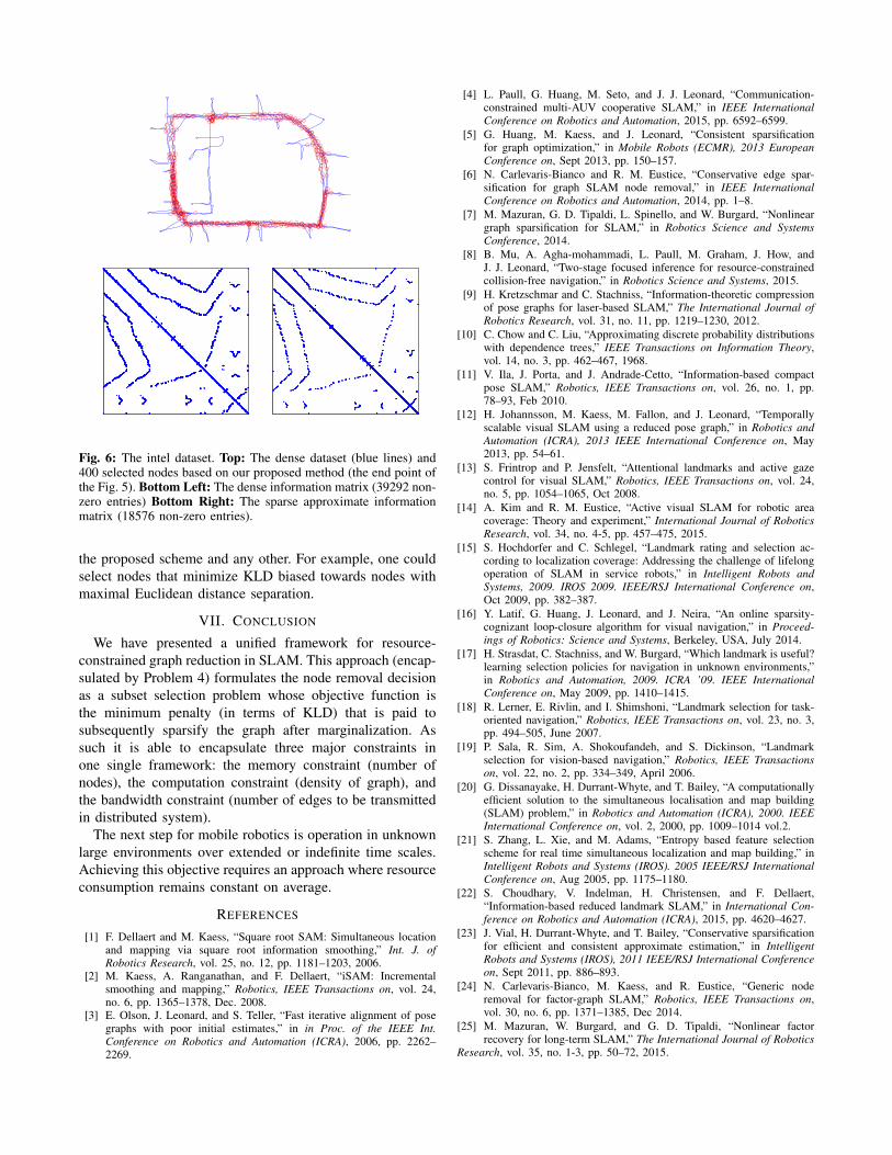
Fig. 6: The intel dataset. Top: The dense dataset (blue lines) and400 selected nodes based on our proposed method (the end point ofthe Fig. 5). Bottom Left: The dense information matrix (39292 non-zero entries) Bottom Right: The sparse approximate informationmatrix (18576 non-zero entries).

the proposed scheme and any other. For example, one couldselect nodes that minimize KLD biased towards nodes withmaximal Euclidean distance separation.

VII. CONCLUSION

We have presented a unified framework for resource-constrained graph reduction in SLAM. This approach (encap-sulated by Problem 4) formulates the node removal decisionas a subset selection problem whose objective function isthe minimum penalty (in terms of KLD) that is paid tosubsequently sparsify the graph after marginalization. Assuch it is able to encapsulate three major constraints inone single framework: the memory constraint (number ofnodes), the computation constraint (density of graph), andthe bandwidth constraint (number of edges to be transmittedin distributed system).

The next step for mobile robotics is operation in unknownlarge environments over extended or indefinite time scales.Achieving this objective requires an approach where resourceconsumption remains constant on average.

REFERENCES

[1] F. Dellaert and M. Kaess, “Square root SAM: Simultaneous locationand mapping via square root information smoothing,” Int. J. ofRobotics Research, vol. 25, no. 12, pp. 1181–1203, 2006.

[2] M. Kaess, A. Ranganathan, and F. Dellaert, “iSAM: Incrementalsmoothing and mapping,” Robotics, IEEE Transactions on, vol. 24,no. 6, pp. 1365–1378, Dec. 2008.

[3] E. Olson, J. Leonard, and S. Teller, “Fast iterative alignment of posegraphs with poor initial estimates,” in in Proc. of the IEEE Int.Conference on Robotics and Automation (ICRA), 2006, pp. 2262–2269.

[4] L. Paull, G. Huang, M. Seto, and J. J. Leonard, “Communication-constrained multi-AUV cooperative SLAM,” in IEEE InternationalConference on Robotics and Automation, 2015, pp. 6592–6599.

[5] G. Huang, M. Kaess, and J. Leonard, “Consistent sparsificationfor graph optimization,” in Mobile Robots (ECMR), 2013 EuropeanConference on, Sept 2013, pp. 150–157.

[6] N. Carlevaris-Bianco and R. M. Eustice, “Conservative edge spar-sification for graph SLAM node removal,” in IEEE InternationalConference on Robotics and Automation, 2014, pp. 1–8.

[7] M. Mazuran, G. D. Tipaldi, L. Spinello, and W. Burgard, “Nonlineargraph sparsification for SLAM,” in Robotics Science and SystemsConference, 2014.

[8] B. Mu, A. Agha-mohammadi, L. Paull, M. Graham, J. How, andJ. J. Leonard, “Two-stage focused inference for resource-constrainedcollision-free navigation,” in Robotics Science and Systems, 2015.

[9] H. Kretzschmar and C. Stachniss, “Information-theoretic compressionof pose graphs for laser-based SLAM,” The International Journal ofRobotics Research, vol. 31, no. 11, pp. 1219–1230, 2012.

[10] C. Chow and C. Liu, “Approximating discrete probability distributionswith dependence trees,” IEEE Transactions on Information Theory,vol. 14, no. 3, pp. 462–467, 1968.

[11] V. Ila, J. Porta, and J. Andrade-Cetto, “Information-based compactpose SLAM,” Robotics, IEEE Transactions on, vol. 26, no. 1, pp.78–93, Feb 2010.

[12] H. Johannsson, M. Kaess, M. Fallon, and J. Leonard, “Temporallyscalable visual SLAM using a reduced pose graph,” in Robotics andAutomation (ICRA), 2013 IEEE International Conference on, May2013, pp. 54–61.

[13] S. Frintrop and P. Jensfelt, “Attentional landmarks and active gazecontrol for visual SLAM,” Robotics, IEEE Transactions on, vol. 24,no. 5, pp. 1054–1065, Oct 2008.

[14] A. Kim and R. M. Eustice, “Active visual SLAM for robotic areacoverage: Theory and experiment,” International Journal of RoboticsResearch, vol. 34, no. 4-5, pp. 457–475, 2015.

[15] S. Hochdorfer and C. Schlegel, “Landmark rating and selection ac-cording to localization coverage: Addressing the challenge of lifelongoperation of SLAM in service robots,” in Intelligent Robots andSystems, 2009. IROS 2009. IEEE/RSJ International Conference on,Oct 2009, pp. 382–387.

[16] Y. Latif, G. Huang, J. Leonard, and J. Neira, “An online sparsity-cognizant loop-closure algorithm for visual navigation,” in Proceed-ings of Robotics: Science and Systems, Berkeley, USA, July 2014.

[17] H. Strasdat, C. Stachniss, and W. Burgard, “Which landmark is useful?learning selection policies for navigation in unknown environments,”in Robotics and Automation, 2009. ICRA ’09. IEEE InternationalConference on, May 2009, pp. 1410–1415.

[18] R. Lerner, E. Rivlin, and I. Shimshoni, “Landmark selection for task-oriented navigation,” Robotics, IEEE Transactions on, vol. 23, no. 3,pp. 494–505, June 2007.

[19] P. Sala, R. Sim, A. Shokoufandeh, and S. Dickinson, “Landmarkselection for vision-based navigation,” Robotics, IEEE Transactionson, vol. 22, no. 2, pp. 334–349, April 2006.

[20] G. Dissanayake, H. Durrant-Whyte, and T. Bailey, “A computationallyefficient solution to the simultaneous localisation and map building(SLAM) problem,” in Robotics and Automation (ICRA), 2000. IEEEInternational Conference on, vol. 2, 2000, pp. 1009–1014 vol.2.

[21] S. Zhang, L. Xie, and M. Adams, “Entropy based feature selectionscheme for real time simultaneous localization and map building,” inIntelligent Robots and Systems (IROS). 2005 IEEE/RSJ InternationalConference on, Aug 2005, pp. 1175–1180.

[22] S. Choudhary, V. Indelman, H. Christensen, and F. Dellaert,“Information-based reduced landmark SLAM,” in International Con-ference on Robotics and Automation (ICRA), 2015, pp. 4620–4627.

[23] J. Vial, H. Durrant-Whyte, and T. Bailey, “Conservative sparsificationfor efficient and consistent approximate estimation,” in IntelligentRobots and Systems (IROS), 2011 IEEE/RSJ International Conferenceon, Sept 2011, pp. 886–893.

[24] N. Carlevaris-Bianco, M. Kaess, and R. Eustice, “Generic noderemoval for factor-graph SLAM,” Robotics, IEEE Transactions on,vol. 30, no. 6, pp. 1371–1385, Dec 2014.

[25] M. Mazuran, W. Burgard, and G. D. Tipaldi, “Nonlinear factorrecovery for long-term SLAM,” The International Journal of Robotics

Research, vol. 35, no. 1-3, pp. 50–72, 2015.