librobotics reference -...

librobotics Reference

xWR

xWF

xRF

Kai O. Arras

Social Robotics Lab

University of Freiburg, Germany

Version 1.0, October 2009

Contents

1 About librobotics 2

2 Reference 2

2.1 chi2invtable . . . . . . . . . . . . . . . . . . . . . . . . . . . . . 2

2.2 compound . . . . . . . . . . . . . . . . . . . . . . . . . . . . . . . 3

2.3 diffangle . . . . . . . . . . . . . . . . . . . . . . . . . . . . . . . 4

2.4 normangle . . . . . . . . . . . . . . . . . . . . . . . . . . . . . . . 4

2.5 drawarrow . . . . . . . . . . . . . . . . . . . . . . . . . . . . . . . 5

2.6 drawellipse . . . . . . . . . . . . . . . . . . . . . . . . . . . . . 6

2.7 drawlabel . . . . . . . . . . . . . . . . . . . . . . . . . . . . . . . 7

2.8 drawprobellipse . . . . . . . . . . . . . . . . . . . . . . . . . . 8

2.9 drawreference . . . . . . . . . . . . . . . . . . . . . . . . . . . . 9

2.10 drawrobot . . . . . . . . . . . . . . . . . . . . . . . . . . . . . . . 10

2.11 drawrect . . . . . . . . . . . . . . . . . . . . . . . . . . . . . . . 12

2.12 drawtransform . . . . . . . . . . . . . . . . . . . . . . . . . . . . 13

2.13 icompound . . . . . . . . . . . . . . . . . . . . . . . . . . . . . . . 14

2.14 j1comp . . . . . . . . . . . . . . . . . . . . . . . . . . . . . . . . . 15

2.15 j2comp . . . . . . . . . . . . . . . . . . . . . . . . . . . . . . . . . 15

2.16 jinv . . . . . . . . . . . . . . . . . . . . . . . . . . . . . . . . . . 16

2.17 mahalanobis . . . . . . . . . . . . . . . . . . . . . . . . . . . . . 17

2.18 meanwm . . . . . . . . . . . . . . . . . . . . . . . . . . . . . . . . . 18

1

1 About librobotics

For the sake of brevity, here just the facts:

• librobotics is a small library with frequently used Octave/Matlab functionsin Robotics, especially for visualization.

• All commands are fully documented, just type help command.

• librobotics is compatible with both, Matlab and Octave.

• It’s open source, feel free to distribute and extend.

• librobotics was written by Kai Arras mainly in 2003-4 as part of the CASRobot Navigation Toolbox. Minor adaptations since then.

• librobotics can be downloaded from the Social Robotics Lab homepage athttp://srl.informatik.uni-freiburg.de/downloads

Enjoy!

2 Reference

2.1 chi2invtable

Lookup table of the inverse of the χ2 cumulative distribution function.

x = chi2invtable(p,v) returns the inverse of the χ2 cumulative distributionfunction (cdf) with v degrees of freedom at the value p. The χ2 cdf with vdegrees of freedom, is the Γ cdf with parameters v/2 and 2.

Opposed to chi2inv of the Matlab statistics toolbox (which might be not partof your Matlab installation), chi2invtable is a lookup table and thereby muchfaster than chi2inv. However, as any lookup table is a collection of samplepoints, accuracy is smaller. Between the sample points of the cdf, a linearinterpolation is made.

Currently, the function supports the degrees of freedom v between 1 and 10 andthe probability levels p between 0 and 0.9999 in steps of 0.0001 plus the level0.99999.

Example: A typical usage scenario of chi2invtable (or chi2inv) is duringthe matching step of a Kalman filter localization or slam cycle. Given theprobability α and features of dimension n, chi2invtable yields the maximalMahalanobis distance (or gate distance) χ2

n,α which a candidate pairing withinnovation νij and innovation covariance Sij may have in order to be accepted.In other words, the pairing is accepted if the following holds:

νTij Sij νij < χ2

n,α

See also chi2inv.

2

http://srl.informatik.uni-freiburg.de/downloads

2.2 compound

Compound relationship in 2D.

xik = compound(xij,xjk) returns the compound relationship of the two 2Dtransforms xij and xjk which are arranged head-to-tail. x’s are 3 × 1-vectors[x, y, θ]T , orientations within [0..2π[.

Example: Given the transform xWR which expresses entity R in the referenceframe of W and transform xRS which represents entity S in the frame of R,then the composition xWS is the relationship which expresses S in the frame ofW :

xWS = xWR ⊕ xRS

Note that the compound operation would be the same as vector addition if therewere no orientations.

xWR

xRS

xWS

Figure 1: compound.m

Reference: R. Smith, M. Self, P. Cheeseman, ”Estimating Uncertain SpatialRelationships in Robotics,” in Autonomous Robot Vehicles, I.J. Cox and G.T.Wilfong, Eds.: Springer-Verlag, 1990, pp. 167-193.

See also icompound, j1comp, j2comp.

3

2.3 diffangle

Take difference of two angles and unwrap it.

α = diffangle(α1,α2) determines the minimal difference α = α1−α2 betweentwo angles α1 and α2. If either α1 or α2 is Inf, Inf is returned.

Example: The difference of α1 = 107.54 and α2 = −115.97 is α = −136.49.

α1

α2

α1 [deg] = 107.5391α2 [deg] = -115.9741

α1- α2 = -136.4867

Figure 2: diffangle.m

See also normangle.

2.4 normangle

Put angle into a 2π interval.

ar = normangle(a,min) puts angle a into the interval [min..min+2π[. If a isInf, Inf is returned.

See also diffangle.

4

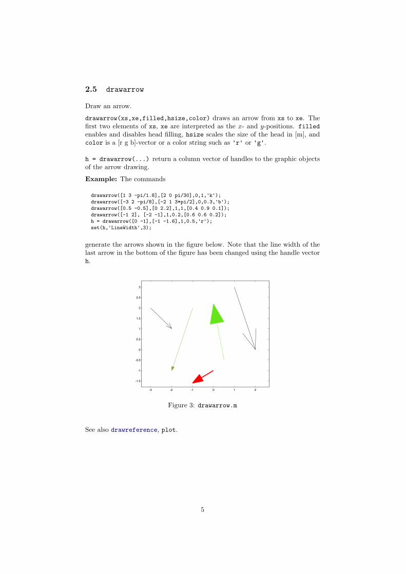
2.5 drawarrow

Draw an arrow.

drawarrow(xs,xe,filled,hsize,color) draws an arrow from xs to xe. Thefirst two elements of xs, xe are interpreted as the x- and y-positions. filledenables and disables head filling, hsize scales the size of the head in [m], andcolor is a [r g b]-vector or a color string such as 'r' or 'g'.

h = drawarrow(...) return a column vector of handles to the graphic objectsof the arrow drawing.

Example: The commands

drawarrow([1 3 -pi/1.8],[2 0 pi/30],0,1,'k');

drawarrow([-3 2 -pi/8],[-2 1 3*pi/2],0,0.3,'b');

drawarrow([0.5 -0.5],[0 2.2],1,1,[0.4 0.9 0.1]);

drawarrow([-1 2], [-2 -1],1,0.2,[0.6 0.6 0.2]);

h = drawarrow([0 -1],[-1 -1.6],1,0.5,'r');

set(h,'LineWidth',3);

generate the arrows shown in the figure below. Note that the line width of thelast arrow in the bottom of the figure has been changed using the handle vectorh.

-3 -2 -1 0 1 2

-1.5

-1

-0.5

0

0.5

1

1.5

2

2.5

3

Figure 3: drawarrow.m

See also drawreference, plot.

5

2.6 drawellipse

Draw ellipse.

drawellipse(x,a,b,color) draws an ellipse at x = [x, y, θ]T with half axes aand b. Orientation θ is the inclination angle of a, regardless if a is smaller orgreater than b. color is a [r g b]-vector or a color string such as 'r' or 'g'.

h = drawellipse(...) returns the graphic handle h.


plot(1,-0.4,'k+');

drawellipse([1 -0.4 pi/6],1,0.5,'k')

plot(0.5,0,'k+');

drawellipse([0.5 0 pi/6],0.25,0.5,'b');

plot(1.8,-0.8,'k+');

h = drawellipse([1.8 -0.8 pi/6],0.2,0.2,[0 0.7 0.3]);

set(h,'LineStyle','-.');

generate the ellipses shown below. Note that the line style of the circle can bechanged using the handle vector h.

0 0.2 0.4 0.6 0.8 1 1.2 1.4 1.6 1.8 2

-1

-0.5

0

0.5

Figure 4: drawellipse.m

See also drawprobellipse.

6

2.7 drawlabel

Draw scalable text.

drawlabel(x,str,scale,offset,color) draws scalable text str at pose x =[x, y, θ]T imitating the OCR font. With scale = 1, the height of the letters is1 meter. offset shifts the text in [m] from the x, y position in postive x- andy-direction. color is either a [r g b]-vector or a color string such as 'r' or 'g'.

Currently, the following characters are implemented: 0, 1, 2, 3, 4, 5, 6, 7, 8, 9,W, R, S, E, F, M, P.

h = drawlabel(...) returns a column vector of handles to all line objects ofthe drawing, one handle per line.


plot(-3,2,'k+'); drawlabel([-3 2 0],'123',0.5,0.0,'k');



plot(-1,2,'k+'); drawlabel([-1,2 -2.8],'R1',0.2,0.1,[.5 .5 .5]);

plot( 1,3,'k+'); drawlabel([ 1 3 -pi/1.8],'F30493',0.8,0.3,'g');

plot(-2,-1,'k+'); h = drawlabel([-2 -1 2.6],'S04',0.3,0.1,'r');


plot(-1,-2,'k+'); h = drawlabel([-1 -2 pi/3],'REF',0.3,0.1,'m');


generate the figure shown below. Note that line width can be varied using thehandle vector h.

-3 -2 -1 0 1 2

-2

-1.5

-1

-0.5

0

0.5

1

1.5

2

2.5

3

Figure 5: drawlabel.m

See also text.

7

2.8 drawprobellipse

Draw elliptic probability region of a Gaussian in 2D.

drawprobellipse(x,C,alpha,color) draws the elliptic iso-probability contourof a Gaussian distributed bivariate random vector x at the significance levelalpha. The ellipse is centered at x = [x, y]T where C is the associated 2 × 2covariance matrix. color is a [r g b]-vector or a color string such as 'r' or 'g'.

x and C can also be of size 3× 1 and 3× 3 respectively.

The function uses chi2invtable instead of chi2inv from the Matlab statisticstoolbox.

In case of a negative definite matrix C, the ellipse collapses to a line which isdrawn instead.

h = drawprobellipse(...) returns the graphic handle h.


x1 = [ 1,2]; C1 = [0.25 -0.2; -0.2 0.3];

drawprobellipse(x1,C1,0.95,'k');

x2 = [-1,0]; C2 = [0.3 -0.03; -0.03 0.01];


x3 = [-2,3]; C3 = [0.01 0.005; 0.005 0.015];


generate the ellipses shown below. Note that line width can be varied using thehandle vector h.

-3 -2 -1 0 1 2 3 -1

-0.5

0

0.5

1

1.5

2

2.5

3

3.5

4

Figure 6: drawprobellipse.m

See also drawellipse, chi2invtable, chi2inv.

8

2.9 drawreference

Draw coordinate reference frame.

drawreference(x,label,size,color) draws a reference frame at pose x =[x, y, θ]T and labels it with the string label. size is the length of the frameaxes in [m], and color is a [r g b]-vector or a color string such as 'r' or 'g'.

h = drawreference(...) returns a column vector of handles to all graphicobjects of the drawing. Remember that not all graphic properties apply to alltypes of graphic objects. Use findobj to find and access the individual objects.


drawreference([0 2 pi/8],'W',1,'k');

drawreference([0 0 pi/3],'R2',0.4,'b');

drawreference([0.8 1.3 -1.8],'S43',0.5,[.8 .5 .1]);

drawreference([2 2.3 -0.3],'',0.6,[.6 .6 .6]);

h = drawreference([2 0.7 pi/9],'98',0.8,[.3 .7 .3]);


generate the figure shown below. Note that line width, line style and color canbe varied using the handle vector h.

-0.5 0 0.5 1 1.5 2 2.5 3

0

0.5

1

1.5

2

2.5

3

Figure 7: drawreference.m

See also drawarrow, drawlabel, findobj, plot.

9

2.10 drawrobot

Draw robot.

drawrobot(x,color) draws a robot at pose x = [x, y, θ]T such that the robotreference frame is attached to the center of the wheelbase with the x-axis lookingforward. color is a [r g b]-vector or a color string such as 'r' or 'g'.

drawrobot(x,color,type) draws a robot of type type. Five different modelsare implemented:

type = 0 draws only a cross with orientation θtype = 1 is a differential drive robot without contourtype = 2 is a differential drive robot with round shapetype = 3 is a round shaped robot with a line at θtype = 4 is a differential drive robot with rectangular shapetype = 5 is a rectangular shaped robot with a line at θ

drawrobot(x,color,type,w,l) draws a robot of type type with width w andlength l in [m].

h = drawrobot(...) returns a column vector of handles to all graphic objectsof the robot drawing. Remember that not all graphic properties apply to alltypes of graphic objects. Use findobj to find and access the individual objects.

0 1 2 3 4 5 -2.5

-2

-1.5

-1

-0.5

0

0.5

1

1.5

2

2.5

Figure 8: drawrobot.m


drawrobot([0 1 1.5],'k',0);

drawrobot([1 1 1.4],'k',1);

drawrobot([2 1 1.3],'k',2);

drawrobot([3 1 1.2],'k',3);

drawrobot([4 1 1.1],'k',4);

drawrobot([5 1 1.0],'k',5);

drawrobot([0 -0.8 2.0],'r',2,0.6,0.6);

drawrobot([1 -1.2 1.9],[.5 .5 .4],4,0.5,0.3);

drawrobot([2 -0.8 1.8],[.7 .5 .4],1,0.2,0.8);

10

drawrobot([3 -1.2 1.7],[.9 .5 .4],5,0.3,0.7);

h = drawrobot([4 -0.8 1.6],'g',3,0.4,0.1);


h = drawrobot([5 -1.2 1.5],'k',0,0.4,0.1);

set(h,'LineWidth',2,'LineStyle',':');

generate the robots shown above. Note that line width, line style and color canbe varied using the handle vector h.

See also drawrect, drawarrow, findobj, plot.

11

2.11 drawrect

Draw rounded rectangle.

drawrect(x,w,h,r,filled,color) draws a rectangle with round corners ofradius r, width w and height h, centered at pose x where x is the 3 × 1 vector[x, y, θ]T . With filled = 1 the rectangle is filled with color color, with filled= 0 only the contour is drawn. color is a [r g b]-vector or a Matlab color stringsuch as 'r' or 'g'.

Note that 2r must be greater or equal than the smaller of the two values w, h.For 2r = w = h, drawrect draws a circle.

h = drawrect(...) returns the graphic handle h.


drawrect([0.4 1 2.6],1,0.6,0.2,0,'b');

drawrect([1.9 2 2.5],1,1.2,0.1,1,[.4 .9 .0]);

drawrect([1.9 2 2.5],1,1.2,0.1,0,[.2 .7 .0]);

drawrect([3.0 1 2.4],0.2,1.7,0.0,0,'r');

drawrect([4.0 0 2.3],0.4,0.4,0.2,1,[.8 .8 .8]);

h = drawrect([4 0 2.3],0.4,0.4,0.2,0,'k');


h = drawrect([5 1 0.6],0.3,0.7,0.15,0,[.9 .7 .0]);


generates the figure shown below. Note that line width, line style and color canbe varied using the handle vector h.

0 0.5 1 1.5 2 2.5 3 3.5 4 4.5 5

-1

-0.5

0

0.5

1

1.5

2

2.5

3

3.5

Figure 9: drawrect.m


12

2.12 drawtransform

Illustrates a spatial relationship.

drawtransform(xs,xe,shape,label,color) draws a nice looking curved ar-row from location xs (3× 1) to xe (3× 1) and labels it with the string label.color is a [r g b]-vector or a Matlab color string such as 'r' or 'g'. shapecontrols the shape of the curve: '/' for a S-shape, '\' for a Z-shape, '(' for aleft arc and ')' for a right arc.

h = drawtransform(...) returns a column vector of handles to all graphicobjects of the drawing. Remember that not all graphic properties apply to alltypes of graphic objects.


plot(0,0,'k+'); plot(0.2, 1.5,'k+');

drawtransform([0 0],[0.2 1.5],'/','x1',[.9 .8 .0]);

plot(1,0,'k+'); plot(1.2, 1.5,'k+');

drawtransform([1 0],[1.2 1.5],'\','x2',[.7 .6 .0]);

plot(2,0,'k+'); plot(2.2, 1.5,'k+');

drawtransform([2 0],[2.2 1.5],'(','x3',[.5 .3 .0]);

plot(3,0,'k+'); plot(3.2, 1.5,'k+');

drawtransform([3 0],[3.2 1.5],')','x4',[.3 .0 .0]);

h = drawtransform([0 0],[2 0],')','','k');

set(h,'LineStyle','--');

h = drawtransform([1 0],[3 0],')','','k');

set(h,'LineStyle',':');

generate the arrows shown below. Note that line width, line style and color canbe set using the handle vector h.

0 0.5 1 1.5 2 2.5 3

-0.5

0

0.5

1

1.5

2

x1 x2 x3x4

Figure 10: drawtransform.m


13

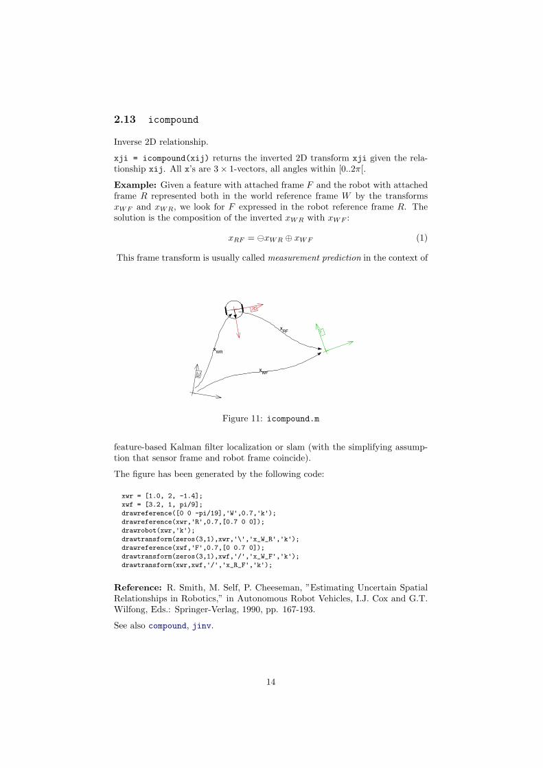
2.13 icompound

Inverse 2D relationship.

xji = icompound(xij) returns the inverted 2D transform xji given the rela-tionship xij. All x’s are 3× 1-vectors, all angles within [0..2π[.

Example: Given a feature with attached frame F and the robot with attachedframe R represented both in the world reference frame W by the transformsxWF and xWR, we look for F expressed in the robot reference frame R. Thesolution is the composition of the inverted xWR with xWF :

xRF = xWR ⊕ xWF (1)

This frame transform is usually called measurement prediction in the context of

xWR

xWF

xRF

Figure 11: icompound.m

feature-based Kalman filter localization or slam (with the simplifying assump-tion that sensor frame and robot frame coincide).

The figure has been generated by the following code:

xwr = [1.0, 2, -1.4];

xwf = [3.2, 1, pi/9];

drawreference([0 0 -pi/19],'W',0.7,'k');

drawreference(xwr,'R',0.7,[0.7 0 0]);

drawrobot(xwr,'k');

drawtransform(zeros(3,1),xwr,'\','x_W_R','k');

drawreference(xwf,'F',0.7,[0 0.7 0]);

drawtransform(zeros(3,1),xwf,'/','x_W_F','k');

drawtransform(xwr,xwf,'/','x_R_F','k');

Reference: R. Smith, M. Self, P. Cheeseman, ”Estimating Uncertain SpatialRelationships in Robotics,” in Autonomous Robot Vehicles, I.J. Cox and G.T.Wilfong, Eds.: Springer-Verlag, 1990, pp. 167-193.

See also compound, jinv.

14

2.14 j1comp

First Jacobian of the compound operator.

J = j1comp(xi,xj) returns the Jacobian matrix of the 2D composition of xiand xj derived with respect to the first operand xi. All x’s are 3× 1-vectors, Jis a 3× 3-matrix.

The Jacobian is used to perform first-order error propagation when the inputtransforms x̂ij and x̂jk of the composition x̂ik = x̂ij ⊕ x̂jk are uncertain. Tocalculate the uncertainty of the output x̂ik, the compound operator is derivatedwith respect to the two operands yielding a 3 × 6 Jacobian matrix J⊕ whichconsists of a left 3× 3 half, J1⊕, and a right 3× 3 half, J2⊕.

J1⊕ =δx̂ik

δxij

∣∣∣∣x̂ij

J2⊕ =δx̂ik

δxjk

∣∣∣∣x̂jk

J⊕ = [J1⊕ J2⊕]

With Cijk as the input covariance matrix

Cijk =[

Cij Cijjk

Cjkij Cjk

]the covariance matrix of the output transform Cik is given by the error propa-gation law

Cik = J⊕CijkJT⊕

= J1⊕CijJT1⊕ + J1⊕CijjkJT

2⊕ + J2⊕CjkijJT1⊕ + J2⊕CjkJT

2⊕

where the submatrix Cijjk (= CjkijT ) is the cross-correlation between x̂ij and

x̂jk.

See also j2comp, jinv, compound, icompound.

2.15 j2comp

Second Jacobian of the compound operator.

J = j2comp(xi,xj) returns the Jacobian matrix of the 2D composition of xiand xj derived with respect to the second operand xj. All x’s are 3× 1-vectors,J is a 3× 3-matrix.

See explanation at j1comp.

See also j1comp, jinv, compound, icompound.

15

2.16 jinv

Jacobian of the inverse compound operator.

J = jinv(xij) returns the Jacobian matrix of the inversion xji of xij. All x’sare 3× 1-vectors.

The Jacobian is used to perform first-order error propagation when the inputtransform x̂ij of the inversion x̂ji = x̂ij is uncertain. To calculate the un-certainty of the output x̂ji, the inverse compound operator is derivated withrespect to the operand yielding the 3× 3 Jacobian matrix J.

J =δx̂ji

δxij

∣∣∣∣x̂ij

With Cij as the input covariance matrix, the covariance matrix of the outputtransform, Cji, is given by the error propagation law

Cji = JCijJT

See also j1comp, j2comp, compound, icompound.

16

2.17 mahalanobis

Calculate the Mahalanobis distance.

d = mahalanobis(v,S) calculates the chi square distributed Mahalanobis dis-tance given the innovation vector v and the innovation covariance matrix S.

Formally, with the innovation ν and the innovation covariance matrix S, theMahalanobis distance is

D = νT S ν (2)

The Mahalanobis distance is a quadratic form and allows to test on positivedefiniteness of a matrix S. With any ν 6= 0, S is positive definite if D > 0 andpositive semidefinite if D ≥ 0.

See also chi2invtable, chi2inv.

17

2.18 meanwm

Multivariate weighted mean (Information Filter).

[xw,Cw] = meanwm(x,C) calculates the multivariate weighted mean. x is amatrix of dimension m × n where each column is interpreted as a Gaussiandistributed random vector of dimension m× 1. C is a m×m× n matrix whereeach m ×m matrix is interpreted as the covariance estimate associated to itsrespective row vector. The function returns the weighted mean vector xw andthe weighted covariance matrix Cw of dimensions m× 1 and m×m respectively.

The multivariate weighted mean is also known as the Information Filter (IF),a batch formulation of the (recursive) Kalman filter. Given the random vectorsx1, x2, ..., xn with associated covariance matrices C1, C2, ..., Cn, the IF calculates

xw = Cw

∑C−1

i xi

C−1w =

∑C−1

i

-0.5 0 0.5 1 1.5 2 2.5 3 3.5 4

0

0.5

1

1.5

2

2.5

3

3.5

Figure 12: meanwm.m

Example: The Matlab code

x1 = [1.5; 1]; C1 = [0.08 -0.082; -0.082 0.1];

drawprobellipse(x1,C1,0.95,[.9 .5 0]);

plot(x1(1),x1(2),'+','Color',[.9 .5 0]);

x2 = [1; 0]; C2 = [0.18 -0.02; -0.02 0.01];

drawprobellipse(x2,C2,0.95,[.9 .2 0]);

plot(x2(1),x2(2),'+','Color',[.9 .2 0]);

xin = cat(2,x1,x2); Cin = cat(3,C1,C2);

[xw,Cw] = meanwm(xin,Cin);

drawprobellipse(xw,Cw,0.95,'k');

plot(xw(1),xw(2),'k+');

x3 = [3; 3]; C3 = [0.01 0.005; 0.005 0.015];

drawprobellipse(x3,C3,0.95,[0 .9 .7]);

plot(x3(1),x3(2),'+','Color',[0 .9 .7]);

18

x4 = [3.2; 2.3]; C4 = [0.03 -0.005; -0.005 0.015];


plot(x4(1),x4(2),'+','Color',[0 .9 .4]);

x5 = [2.5; 2.4]; C5 = [0.005 -0.002; -0.002 0.008];


plot(x5(1),x5(2),'+','Color',[0 .9 .1]);

xin = cat(2,x3,x4,x5); Cin = cat(3,C3,C4,C5);

[xw,Cw] = meanwm(xin,Cin);

drawprobellipse(xw,Cw,0.95,'k');

plot(xw(1),xw(2),'k+');

generates the figure shown below. Note how the command cat is used to preparethe input arguments.

See also mean, cat, drawprobellipse.

19

librobotics reference -...

Documents