lidia: lightweight learned image denoising with instance ... · lidia: lightweight learned image...
TRANSCRIPT

LIDIA: Lightweight Learned Image Denoising with Instance Adaptation
Gregory Vaksman
CS Department - The Technion
Michael Elad
Google Research
Peyman Milanfar
Google Research
Abstract
Image denoising is a well studied problem with an exten-
sive activity that has spread over several decades. Leading
classical denoising methods are typically designed to ex-
ploit the inner structure in images by modeling local over-
lapping patches, and operating in an unsupervised fashion.
In contrast, newcomers to this arena are supervised and
universal neural-network-based methods that bypass this
modeling altogether, targeting the inference goal directly
and globally, tending to be deep and parameter heavy.
This work proposes a novel lightweight learnable ar-
chitecture for image denoising, using a combination of
supervised and unsupervised training of it, the first aim-
ing for a universal denoiser and the second for an in-
stance adaptation. Our architecture embeds in it concepts
taken from classical methods, leveraging patch process-
ing, non-local self-similarity, representation sparsity and
a multiscale treatment. Our proposed universal denoiser
achieves near state-of-the-art results, while using a small
fraction of the typical number of parameters. In addi-
tion, we introduce and demonstrate two highly effective
ways for further boosting the denoising performance, by
adapting this universal network to the input image. The
code reproducing the results of this paper is available at
https://github.com/grishavak/LIDIA-denoiser.
1. Introduction
Image denoising is a well studied problem, and many
successful algorithms have been developed for handling this
task over the years, e.g. NLM [2], KSVD [11], BM3D [8],
EPLL [52], WNNM [12] and others [36, 24, 47, 9, 32, 28,
15, 35, 43, 45, 40, 29]. These classically-oriented algo-
rithms strongly rely on models that exploit properties of
natural images, usually employed while operating on small
fully overlapped patches. For example, both EPLL [52] and
PLE [47] perform denoising using Gaussian Mixture Mod-
eling (GMM) imposed on the image patches. The K-SVD
algorithm [11] restores images using a sparse modeling of
such patches. BM3D [8] exploits self-similarity by group-
(a) Clean image (b) Noisy (σ = 50)
(c) Denoised
PSNR = 24.33dB
(d) Denoised (after adaptation)
PSNR = 26.25dB
Figure 1: Our adaptation approach: (a) and (b) show the
clean and noisy images; (c) is the denoised result by our
universal architecture (d) presents our externally adapted re-
sult, using an additional single astronomical image.
ing similar patches to 3D blocks and filtering them jointly.
The algorithms reported in [40, 29] harness a multi-scale
analysis framework on top of the above-mentioned local
models. Common to all these and many other classical de-
noising methods is the fact that they operate in an unsuper-
vised fashion, adapting their treatment to each image.
Recently, supervised deep-learning based methods en-
tered the denoising arena, showing state-of-the-art (SOTA)
results in various contexts [3, 6, 44, 48, 25, 49, 34, 41, 23,
50, 22]. In contrast to the above-mentioned classical al-
gorithms, deep-learning based methods tend to bypass the
need for an explicit modeling of image redundancies, op-
erating instead by directly learning the inference from the
incoming images to their desired outputs. In order to ob-
tain a non-local flavor in their treatment, as self-similarity
or multi-scale methods would do, most of these algorithms
([22] being an exception) tend to increase their footprint by
utilizing very deep and parameter heavy networks. These
1
reflect badly on their memory consumption, the required
amount of training images and the time for training and in-
ference. Note that most deep-learning based denoisers oper-
ate in an universal fashion, i.e., they apply the same trained
network to all incoming images.
An interesting recent line of work by Lefkimmiatis pro-
poses a denoising network with a significantly reduced
number of parameters, while persisting on near SOTA per-
formance [18, 19]. This method leverages the non-local
self-similarity property of images by jointly operating on
groups of similar patches. The network’s architecture con-
sists of several repeated stages, each resembling a single
step of the proximal gradient descent method under sparse
modeling [30]. In comparison with DnCNN [48], the work
reported in [18, 19] shows a reduction by factor of 14 in
the number of parameters, while achieving denoising PSNR
that is only ∼ 0.2 dB lower.
In this paper we propose two threads of novelty. Our
first contribution aims at a better design of a denoising net-
work, inspired by Lefkimmiatis’ work. This network is to
be trained in a supervised fashion, creating an effective uni-
versal denoiser for all images. Our second contribution ex-
tends the above by introducing image adaptation: We of-
fer ways for updating the above network for each incoming
image, so as to accommodate better its content and inner
structure, leading to better denoising.
Referring to the first part of this work (our universal de-
noiser), we continue with Lefkimmiatis’ line of lightweight
networks and propose a novel, easy, and learnable archi-
tecture that harnesses several main concepts from clas-
sical methods: (i) Operating on small fully overlapping
patches; (ii) Exploiting non-local self-similarity; (iii) Lever-
aging representation sparsity; and (iv) Employing a multi-
scale treatment. Our network resembles the one proposed
in [18, 19], with several important differences:
• We introduce a multi-scale treatment that combats spa-
tial artifacts, especially noticeable in smooth regions
[40]. While this change does not reflect strongly on
the PSNR results, it has a clear visual contribution;
• Our network is more effective by operating in the
residual domain, similar to the approach taken by [48];
• Our patch fusion operator includes a spatial smooth-
ing, adding an extra force to our overall filtering; and
• Our architecture is trained end-to-end, whereas
Lefkimiatis’s scheme consists of a greedy training of
its layers, followed by an end-to-end update.
Our proposed method operates on all the overlapping
patches taken from the processed image by augmenting
each with its nearest neighbors and filtering these jointly.
The patch grouping stage is applied only once before any
filtering, and it is not a part of the learnable architecture.
Each patch group undergoes a series of trainable steps that
aim to predict the noise in the candidate patch, thereby op-
erating in the residual domain. As mentioned above, our
scheme includes a multi-scale treatment, fusing the process-
ing of corresponding patches from different scales.
Moving to the second novelty in this work (image adap-
tation), we present two ways for updating the universal net-
work for any incoming image, so as to further improve its
denoised result. This part relies on three key observations:
(i) A universally trained denoiser is necessarily less effec-
tive when handling images falling outside the training-set
statistics; (ii) While our universal denoiser does exploit self-
similarity, this can be further boosted for images with pro-
nounced repetitions; and (iii) As our universal denoiser is
lightweight, even a single image example can be used for
updating it without overfitting.
In accordance with these, we propose to retrain the uni-
versal network and better tune it for the image being served.
One option, the external boosting, suggests taking the uni-
versally denoised result, and using it for searching the web
for similar photos. Taking even one such related image and
performing few epochs of update to the network may im-
prove the overall performance. This approach is extremely
successful for images that deviate from the training-set, as
illustrated in Figure 1. The second adaptation technique,1
the internal one, re-trains the network on the denoised im-
age itself (and a noisy version of it). This is found to be
quite effective for images with marked inner-similaries.
To summarize, this paper has two key contributions:
1. We propose a novel architecture that is inspired by
classical denoising algorithms. Employed as a univer-
sal denoiser and trained in a supervised fashion, our
network gives near-SOTA results while using a very
small number of parameters to be tuned 2
2. We present an image-adaptation option, in which the
above network is updated for better treating the incom-
ing image. This adaptation becomes highly effective
in cases of images deviating from the natural image
statistics, or in situations in which the incoming im-
age exhibits stronger inner-structure. In these cases,
denoising results are boosted dramatically, surpassing
known supervised deep-denoisers.
1A recently published work [4, 5] proposes an interesting special ar-
chitecture constraint that allows for training the network on the corrupted
image itself in a fashion similar to our adaptation. We shall return to these
papers in the results’ section and explain more on the relation to our work.2Reducing the number of network parameters is important for low GPU
memory consumption and for reducing the number of images required for
training. Indeed, our proposed adaptation relies on this feature for avoiding
overfitting. We should note, however, that while the number of parameters
in our proposed network is relatively small, our inference computational
load is similar to DnCNNs.

2. The Proposed Universal Network
2.1. Overall Algorithm Overview
Our proposed method extracts all possible overlapping
patches of size√n × √
n from the processed image, and
cleans each in a similar way. The final reconstructed image
is obtained by combining these restored patches via averag-
ing. The algorithm is shown schematically in Figure 2.
In order to formulate the patch extraction, combination
and filtering operations, we introduce some notations. As-
sume that the processed image is of size M × N . We de-
note by Y, Y ∈ RMN the noisy and denoised images re-
spectively, both reshaped to a 1D vector. Similarly, the
corrupted and restored patches in location i are denoted by
zi, zi ∈ Rn respectively, where i = 1, . . . ,MN .3 Patch ex-
traction from the noisy image is denoted by zi = RiY , and
the denoised image is obtained by combining the denoised
patches {zi} using weighted averaging,
Y =
(
∑
i
wiRTi Ri
)
−1∑
i
wiRTi zi, (1)
where these weights are wi = exp {−β · var (zi)},
(var (z) is a sample variance of z, and β is learned).
2.2. Our Scheme: A Closer Look
Zooming in on the local treatment, it starts by augment-
ing the patch zi with a group of its k− 1 nearest neighbors,
forming a matrix Zi of size n × k. The nearest neighbor
search is done using a Euclidean metric, limited to a search
window of size b× b around the center of the patch.
The matrix Zi undergoes a series of trainable operations
that aim to recover a clean candidate patch zi. Our filtering
network consists of several blocks, each consisting of (i) a
forward 2D linear transform; (ii) a non-negative threshold-
ing (ReLU) on the obtained features; and (iii) a transform
back to the image domain. All transforms operate sepa-
rately in the spatial and the similarity domains. In contrast
to BM3D and other methods, our filtering predicts the resid-
ual rather than the clean patches, just as done in [48].
Our scheme includes a multi-scale treatment and a fu-
sion of corresponding patches from the different scales.
The adopted strategy borrows its rationale from [46], which
studied the single image super resolution task. In their algo-
rithm, high-resolution patches and their corresponding low-
resolution versions are jointly treated by assuming that they
share the same sparse representation. The two resolution
patches are handled by learning a pair of coupled dictio-
naries. In a similar fashion, we augment the correspond-
ing patches from the two scales, and learn a joint trans-
form for their fusion. In our experiments, the multi-scale
3We handle boundaries by padding using mirror reflection. Thus, the
number of extracted patches is equal to the number of pixels in the image.
scheme includes only two scales, but the same concept can
be applied to a higher pyramid. In our notations, the 1st
scale is the original noisy image Y, and the 2nd scale im-
ages are created by convolving Y with the low-pass filter
fLP = 116
[
1 2 1]T ·
[
1 2 1]
and down-sampling the
result by a factor of two. In order to synchronize between
patch locations in the two scales, we create four downscaled
images by sampling the convolved image at either even or
odd locations: Y(2)ee ,Y
(2)eo ,Y
(2)oe ,Y
(2)oo (even/odd columns
& even/odd rows). For each 1st scale patch, the correspond-
ing 2nd scale patch (of the same size√n×√
n) is extracted
from the appropriate down-sampled image, such that both
patches are centred at the same pixel in the original image.
We denote the 2nd scale patch that corresponds to zi by
z(2)i ∈ R
n. This patch is augmented with a group of its
k−1 nearest neighbors, forming a matrix Z(2)i of size n×k.
The nearest neighbor search is performed in the same down-
scaled image from which z(2)i is taken.Both matrices, {Zi}
and {Z(2)i }, are fed to the filtering network, which fuses the
scales using a joint transform, as described next.
2.3. The Filtering Network
A basic component within our network is the TRT
(Transform–ReLU–Transform) block, which follows the
classic Thresholding algorithm in sparse approximation the-
ory [10]. The same conceptual structure is employed by the
well-known BM3D [8]. The TRT block applies a learned
transform, non-negative thresholding (ReLU) and another
transform on the resulting matrix. Both transforms are sep-
arable, denoted by the operator T and implemented us-
ing a Separable Linear (SL) layer, T (Z) = SL (Z) =W1ZW2 +B, where W1 and W2 operate in the spatial and
the similarity domains. Separability of SL allows a substan-
tial reduction in the number of parameters. As concatena-
tion of two SL layers can be replaced by a single effective
SL, we remove one SL layer in such concatenations. The
TRT component without the second transform is denoted
by TR, and when concatenating k TRT-s, the first k − 1blocks should be replaced by TR-s. Another variant we use
in our network is TBR, which is a version of TR with batch
normalization added before the ReLU.
Another component of the filtering network is an Ag-
gregation block (AGG). This block imposes consistency
between overlapping patches {zi} by combining them to a
temporary image xtmp using plain averaging and extract-
ing them back from the obtained image by Rixtmp. The
complete architecture of the filtering network is presented
in Figure 3. The network receives as input two sets of ma-
trices, {Zi} and {Z(2)i }, and its output is an array of filtered
overlapping patches {zi}. At first, each of these matrices is
multiplied by a diagonal weight matrix diag(wi)Zi. Recall
that the columns of Zi (or {Z(2)i }) are image patches, where

Figure 2: The proposed denoising Algorithm: Extract overlapping patches and their corresponding reduced-scales; Augment
the patches with their nearest neighbors and filter. Reconstruct by combining all the filtered patches via averaging.
the first is the processed one and the rest are its neighbors.
The weights wi express the network’s belief regarding the
relevance of each of the neighbors to the denoising process.
These weights are calculated using an auxiliary network de-
noted as “weight net”, consisting of seven FC (Fully Con-
nected) layers of size k × k with batch normalization and
ReLU between each two FC’s. The network gets as input
the sample variance of the processed patch and k−1 squared
distances between the patch and its neighbors.
After multiplication by diag(wi) the Zi matrix under-
goes a series of operations that include transforms, ReLUs
and AGG, until it gets to the TBR2 block, as shown in
Figure 3. The aggregation block imposes consistency of
the {Zi} matrices, which represent overlapping patches,
but also causes loss of some information. Thus, we split
the flow into two branches: with and without AGG. Since
the output of any TR or TBR component is in the feature
domain, we wrap the AGG block with Tpre and TRpost,
where Tpre transforms the features to the image domain,
and TRpost transforms the AGG output back to the fea-
ture space, while imposing sparsity. The 2nd scale matri-
ces, {Z(2)i }, undergo very similar operations as the 1st scale
ones, but with different learned parameters.
TBR2 applies a joint transform that fuses the features
coming from four origins: the 1st and 2nd scales with and
without aggregation. The columns of all these matrices are
concatenated together such that the same spatial transforma-
tion W1 is applied on all. Note that the network size can be
reduced at the cost of a slight degradation in performance
by removing the TBR1, TBR(2)1 and TBR3 components.
We discuss this option in the result section.
3. Image Adaptation
The above designed network, once trained, offers a uni-
versal denoising machine, capable of removing white addi-
tive Gaussian noise from all images by applying the same
set of computations to all images. As such, this machine
is not adapted to the incoming image, which might deviate
from the general statistics of the training corpus, or could
have an inner structure that is not fully exploited. This lack
of adaptation may imply reduced denoising performance.
In this section we address this weakness by discussing an
augmentation of our denoising algorithm that leads to such
an adaptation and improved denoising results.
Several recent papers have already proposed techniques
for training networks while only using corrupted exam-
ples [20, 42, 16, 27, 1, 17, 21, 39, 38]. An interesting spe-
cial case is where the network is trained on the corrupted
image itself. Indeed, this single-image unsupervised learn-
ing has been successfully employed by classical algorithms.
For example, The KSVD Denoising algorithm [11] trains a
dictionary using patches extracted from the corrupted im-
age. Another example is PLE [47], in which a GMM is
fitted to the given image. Recent deep learning based meth-
ods [42, 27] adopted this approach, training on the cor-
rupted image. However, their obtained performance tends
to be non-competitive with fully supervised schemes.
This raises an intriguing question: Could deep regression
machines benefit from both supervised and single-image
unsupervised training techniques? In this paper we provide
a positive answer to this question, while leveraging the fact
that our denoising network is lightweight. Our proposed
denoiser is able to combine knowledge learned from an ex-
ternal dataset with knowledge that lies in the currently pro-
cessed image, all while avoiding overfitting. We introduce
two novel types of adaptation techniques, external and in-
ternal, which should remind the reader of transfer learning.
Both adaptation types start by denoising the input image
regularly. Then the network is re-trained and updated for
few epochs. In the external adaptation case, we seek (e.g.,
using Google image search) one or few other images closely
related to the processed one, and re-train the network on
this small set of clean images (and their noisy versions). In
the internal adaptation mode, the network is re-trained on
the denoised image itself using a loss function of the form
‖ fθ(
Y + n
)
− Y ‖22, where Y = fθ (Y ) is the universally
denoised image, and n is a synthetic noise. For both ex-

Figure 3: The filtering network
ternal and internal adaptations the procedure concludes by
denoising the input image by the updated network. 4
While the two adaptation methods seem similar, they
serve different needs. External adaptation should be cho-
sen when handling images with special content that is not
well represented in the training set. For example, this mode
could be applied on non-natural images such as scanned
documents. Processing images with special content could
be handled by training class-aware denoisers, however this
might require a large amount of images for training each
class, and holding many networks for covering the vari-
ety of classes to handle. For example, [33, 34] train their
networks on 900 images per class. In contrast, our ex-
ternal adaptation requires a single network for all images,
while updating it for each incoming image. In Section 5 we
present denoising experiments, in which applying external
adaptation gains substantial improvement of more than 1dB
in terms of PSNR. In contrast to external adaptation, the in-
ternal one becomes effective when the incoming image is
characterized by a high level of self-similarity. For exam-
ple, as shown in Section 5, applying internal adaptation on
images from Urban 100 [13] gains a notable improvement
of almost 0.3dB in PSNR on average. Note that these adap-
tation procedures are not always successful. However, fail-
ures usually do not cause performance degradation, indicat-
ing that these procedures, in the context of being deployed
on a lightweight network, do not overfit. Indeed, while we
got a negligible decrease in performance of up to 0.02dB for
few images with the internal adaptation, most unsuccessful
tests led to a marginal increment of at least 0.02− 0.05dB.
4. Experimental Results: Universal Denoising
This section reports the performance of the proposed
scheme, with a comprehensive comparison to recent SOTA
denoising algorithms. In particular, we include in these
comparisons the classical BM3D [8] due to its resemblance
to our network architecture, the TNRD [6], DnCNN [48]
4Our internal adaptation is markedly different from the Noise2Noise
method. While Noise2Noise training requires a dataset of pairs of images
contaminated with independent noise, our internal adaptation requires nei-
ther a dataset nor such pairs, as it trains using the single noisy image.
and FFDNet [49] networks, the non-local and high per-
formance NLRN [22] architecture, and the recently pub-
lished Learned K-SVD (LKSVD) [37] method. We also
include comparisons to Lefkimiatis’ networks, NLNet [18]
and UNLNet [19], which inspired our work. Our algorithm
is denoted as Lightweight Learned Image Denoising with
Instance Adaptation (LIDIA), and we present two versions
of it, LIDIA and LIDIA-S. The second is a simplified net-
work with slightly weaker performance (see more below).
We start with denoising experiments in which the noise
is Gaussian white of known variance. This is the common
case covered by all the above mentioned methods. Our net-
work is trained on 432 images from the BSD500 set [26],
and the evaluation uses the remaining 68 images (BSD68).
The network is trained end-to-end using decreasing learn-
ing rate over batches of 4 images using the MSE loss. We
start training with the Adam optimizer (learning rate 10−2)
and switch to SGD with an initial learning rate of 10−3.
Figure 4 presents a comparison between our algorithm
and leading alternative ones by presenting their PSNR ver-
sus their number of trained parameters. This figure ex-
poses the fact that the performance of denoising networks
is heavily influenced by their complexity. As can be seen,
the various algorithms can be split into two categories:
lightweight architectures with a number of parameters be-
low 100K (TNRD [6], LKSVD [37], NLNet [18] and UNL-
Net, and much larger and slightly better performing net-
works (DnCNN [48], FFDNet [49], and NLRN [22]) that
use hundreds of thousands of parameters. Other SOTA
denoisers published in the past year are FOCNet [14],
RDN+ [51], and N3Net [31]. However, all of these achieve
denoising performance similar to NLRN [22], while be-
longing to the heavier networks category. Therefore, we
show comparisons with NLRN as a representative of this
class of high performing large architectures. As we proceed
in this section, we emphasize lightweight architectures in
our comparisons, a category to which our network belongs.
Figure 4 shows that our networks (both LIDIA and LIDIA-
S) achieve the best results within this lightweight category.
Detailed quantitative denoising results per noise level are

Figure 4: Comparing denoising networks: PSNR perfor-
mance vs. the number of trained parameters (σ = 25).
MethodNoise σ
Average15 25 50
TNRD[6] 31.42 28.92 25.97 28.77
DnCNN[48] 31.73 29.23 26.23 29.06
BM3D[8] 31.07 28.57 25.62 28.42
NLRN[22] 31.88 29.41 26.47 29.25
NLNet1[18] 31.50 28.98 26.03 28.84
NLMS(our) 31.62 29.11 26.17 28.97
Table 1: B/W denoising performance: Best PSNR in red,
and best PSNR within the low-weight category in blue.
DnCNN NLRN TNRD NLNet1 NLMS NLMS-S
556K 330K 26.6K 24.3K 61.6K 40.2K
Table 2: Denoising networks: Number of parameters.
reported5 in Table 1. Table 2 reports the number of trained
parameters per each of the competing networks.
For denoising of color images we use 3D patches of
size 5 × 5 × 3 and increase the size of the matrices W1
from (49 × 64, 64 × 64, 64 × 49) to (75 × 80, 80 × 80,
80 × 75) accordingly, which increases the total number
of our network’s parameters to 94K. The nearest neigh-
bor search is done using the Luminance component, Y =0.2989R+0.5870G+0.1140B. Quantitative denoising re-
sults are reported in Table 3, where our network is denoted
as C-LIDIA (Color LIDIA). As can be seen, our network is
the best within the lightweight category, achieving a similar
performance as CDnCNN [48]. Note, however, that CD-
nCNN is no longer SOTA for color images, as RDN+ [51]
achieves 0.2 − 0.3dB higher PSNR. Figure 5 presents an
example of a denoising result. Since our architecture is re-
5 NLNet [18] complexity and PSNR are taken from the released code.
MethodNoise σ
Average15 25 50
FFDNet[49] 33.87 31.21 27.96 31.01
CDnCNN[48] 33.99 31.31 28.01 31.10
CBM3D[7] 33.50 30.68 27.36 30.51
CNLNet1[18] 33.81 31.08 27.73 30.87
C-LIDIA(our) 34.03 31.31 27.99 31.11
Table 3: Color denoising performance: Best PSNR in red,
and best PSNR within the low-weight category in blue.
(a) Original (b) Noisy with σ = 50
(c) CDnCNN [48]
PSNR = 27.81dB
(d) CBM3D [7]
PSNR = 26.98dB
(e) CNLNet [18]
PSNR = 27.41dB
(f) C-LIDIA (ours)
PSNR = 27.79dB
Figure 5: Color image denoising example with σ = 50.
lated to both BM3D and NLNet, we focus on qualitative
comparisons with these algorithms. Our results are signifi-
cantly sharper with less artifacts and preserve more details
than those of BM3D. In comparison to NLNet, our method
is significantly better in high noise levels due to our multi-
scale treatment, recovering large repeating elements, as in
Figure 5f. Differences between the results are better seen
when zooming in on the region marked with a red rectan-
gle. For more examples see the Supplementary Material.
Blind denoising, i.e., denoising with unknown noise
level, is a useful feature when it comes to neural networks.
This allows using a fixed network for performing image
denoising, while serving a range of noise levels. This is
a more practical solution, when compared to the one dis-
cussed above, in which we have designed a series of net-
works, each trained for a particular σ. We report blind
denoising performance of our architecture and compare to
MethodNoise σ
Average15 25
DnCNN-b[48] 31.61 29.16 30.39
UNLNet[19] 31.47 28.96 30.22
LIDIA-b (ours) 31.54 29.06 30.30
Table 4: Blind denoising performance.
MethodNoise σ
Average15 25 50
LIDIA 31.62 29.11 26.17 28.97
LIDIA-S 31.57 29.08 26.13 28.93
LIDIA-b 31.54 29.06 – 30.30
LIDIA-S-b 31.49 29.01 – 30.25
Table 5: LIDIA vs. its smaller version LIDIA-S.
similar results by DnCNN-b [48] (a version of DnCNN that
has been trained for a range of σ values) and UNLNet [19].
Our blind denoising network (denoted LIDIA-b) preserves
all its structure, but simply trained by mixing noise level
examples in the range 10 ≤ σ ≤ 30. The evaluation of all
three networks is performed on images with σ = [15, 25].The results of this experiment are brought in Table 4. As can
be seen, our method obtains a higher PSNR than UNLNet,
while being slightly weaker than DnCNN-b. Considering
again the fact that our network has nearly 10% of the pa-
rameters of DnCNN-b, we can say that our approach leads
to SOTA results in the lightweight category.
Our LIDIA denoising network can be further simplified
by removing the TBR1, TBR(2)1 and TBR3 components.
The resulting smaller network, denoted by LIDIA-S, con-
tains 30% less parameters than the original LIDIA architec-
ture (see Table 2), while achieving slightly weaker perfor-
mance. Table 5 shows that for both regular and blind de-
noising scenarios, LIDIA-S achieves an average PSNR that
is only 0.05dB lower than the full-size LIDIA network. For
a visual comparison between NLMS and NLMS-S results
see Section 4 of the Supplementary Material.
5. Experimental Results: Network Adaptation
We turn to present results related to external and inter-
nal image adaptation. We compare the performance of our
network (before/after adaptation) with DnCNN [48]. Un-
less said otherwise, all adaptation results are obtained via
5 epochs, requiring few minutes (depending on the image
size) on Nvidia GeForce GTX 1080 Ti GPU. The adaptation
does not require early stopping – over-training the network
leads to similar and sometimes better results.
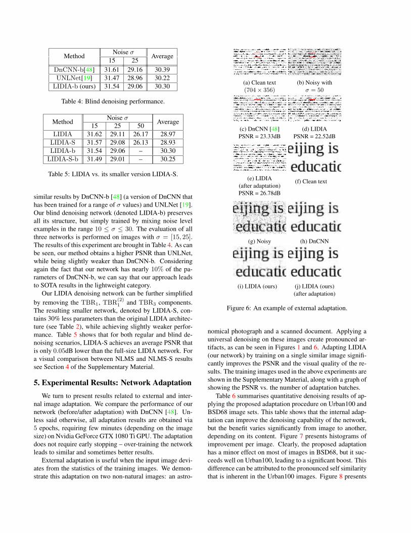
External adaptation is useful when the input image devi-
ates from the statistics of the training images. We demon-
strate this adaptation on two non-natural images: an astro-
(a) Clean text
(704× 356)(b) Noisy with
σ = 50
(c) DnCNN [48]
PSNR = 23.33dB
(d) LIDIA
PSNR = 22.52dB
(e) LIDIA
(after adaptation)
PSNR = 26.78dB
(f) Clean text
(g) Noisy (h) DnCNN
(i) LIDIA (ours) (j) LIDIA (ours)
(after adaptation)
Figure 6: An example of external adaptation.
nomical photograph and a scanned document. Applying a
universal denoising on these images create pronounced ar-
tifacts, as can be seen in Figures 1 and 6. Adapting LIDIA
(our network) by training on a single similar image signifi-
cantly improves the PSNR and the visual quality of the re-
sults. The training images used in the above experiments are
shown in the Supplementary Material, along with a graph of
showing the PSNR vs. the number of adaptation batches.
Table 6 summarises quantitative denoising results of ap-
plying the proposed adaptation procedure on Urban100 and
BSD68 image sets. This table shows that the internal adap-
tation can improve the denoising capability of the network,
but the benefit varies significantly from image to another,
depending on its content. Figure 7 presents histograms of
improvement per image. Clearly, the proposed adaptation
has a minor effect on most of images in BSD68, but it suc-
ceeds well on Urban100, leading to a significant boost. This
difference can be attributed to the pronounced self similarity
that is inherent in the Urban100 images. Figure 8 presents

Image setCDnCNN C-LIDIA C-LIDIA (ours)
[48] (ours) with adaptation
Urban100 28.16 28.23 28.52
BSD68 28.01 27.99 28.04
Table 6: Internal adaptation for color images.
DnCNN FC-AIDE FC-AIDE LIDIA LIDIA
(adapt.) (adapt.)
26.28 25.55 26.42 26.51 26.71
Table 7: Internal adaptation on Urban100 grayscale images.
(a) BSD68 (b) Urban100
Figure 7: Improvements obtained by the internal adaptation.
visual example of the internal adaptation. The image pre-
sented in this figure is characterised by a strong self sim-
ilarity, which our adaptation is able to exploit. As evident
from Figure 7a, internal adaptation is not always successful,
and it may lead to slightly decreased PSNR. However, we
note that among the 168 test images (BSD68 and Urban100)
only two such failures were encountered, both leading to a
degradation of 0.02dB. We conclude that internal adaptation
is robust and cannot do much harm.
N-AIDE [4] and FC-AIDE [5] fine-tune their networks
for each input image in a fashion similar to our adaptation,
by constraining each output pixel to be a polynomial func-
tion of the corresponding input one. As FC-AIDE outper-
forms N-AIDE, we focus on comparing LIDIA to it. Our
network is much lighter – FC-AIDE contains 820K param-
eters while LIDIA uses 62K. Also, FC-AIDE is designed
for grayscale denoising, while LIDIA can handle color as
well. For a quantitative comparison, we run LIDIA with an
internal adaptation on the grayscale Urban100 with σ = 50.
The results of this experiment are brought in Table 7. As can
be seen, LIDIA obtains a higher PSNR in both the universal
and the adapted versions.
6. Conclusion
This work presents a lightweight universal network
for supervised image denoising, demonstrating competitive
performance with SOTA. Our patch-based architecture ex-
ploits non-local self-similarity and representation sparsity,
augmented by a multiscale treatment. Separable linear lay-
ers, combined with non-local k neighbor search, allow cap-
(a) Clean
(1024× 768)(b) Noisy
with σ = 50
(c) CDnCNN [48]
PSNR = 28.64dB
(d) C-LIDIA
PSNR = 28.77dB
(e) C-LIDIA
(after adaptation)
PSNR = 29.28dB
(f) Clean
(g) Noisy (h) CDnCNN
(i) C-LIDIA (ours)
(before adaptation)
(j) C-LIDIA (ours)
(after adaptation)
Figure 8: An example of internal adaptation.
turing non-local interrelations between pixels. In addition,
this work offers two image-adaption techniques, aiming for
improved denoising performance by better tuning the above
universal network to the incoming noisy image. We demon-
strate the effectiveness of these methods on images with
unique content or having significant self-similarity.
References
[1] Joshua Batson and Loic Royer. Noise2self: Blind denoising
by self-supervision. arXiv preprint arXiv:1901.11365, 2019.
4
[2] Antoni Buades, Bartomeu Coll, and J-M Morel. A non-local
algorithm for image denoising. In 2005 IEEE Computer So-
ciety Conference on Computer Vision and Pattern Recogni-
tion (CVPR’05), volume 2, pages 60–65. IEEE, 2005. 1
[3] Harold C Burger, Christian J Schuler, and Stefan Harmeling.
Image denoising: Can plain neural networks compete with
bm3d? In 2012 IEEE conference on computer vision and
pattern recognition, pages 2392–2399. IEEE, 2012. 1
[4] Sungmin Cha and Taesup Moon. Neural adaptive image de-
noiser. In 2018 IEEE International Conference on Acoustics,
Speech and Signal Processing (ICASSP), pages 2981–2985.
IEEE, 2018. 2, 8
[5] Sungmin Cha and Taesup Moon. Fully convolutional pixel
adaptive image denoiser. In Proceedings of the IEEE Inter-
national Conference on Computer Vision, pages 4160–4169,
2019. 2, 8
[6] Yunjin Chen, Wei Yu, and Thomas Pock. On learning
optimized reaction diffusion processes for effective image
restoration. In Proceedings of the IEEE conference on
computer vision and pattern recognition, pages 5261–5269,
2015. 1, 5, 6
[7] Kostadin Dabov, Alessandro Foi, Vladimir Katkovnik, and
Karen Egiazarian. Color image denoising via sparse 3d col-
laborative filtering with grouping constraint in luminance-
chrominance space. In 2007 IEEE International Conference
on Image Processing, volume 1, pages I–313. IEEE, 2007. 6
[8] Kostadin Dabov, Alessandro Foi, Vladimir Katkovnik, and
Karen Egiazarian. Image denoising by sparse 3-d transform-
domain collaborative filtering. IEEE Transactions on image
processing, 16(8):2080–2095, 2007. 1, 3, 5, 6
[9] Weisheng Dong, Lei Zhang, Guangming Shi, and Xin
Li. Nonlocally centralized sparse representation for im-
age restoration. IEEE transactions on Image Processing,
22(4):1620–1630, 2012. 1
[10] Michael Elad. Sparse and redundant representations: from
theory to applications in signal and image processing.
Springer Science & Business Media, 2010. 3
[11] Michael Elad and Michal Aharon. Image denoising via
sparse and redundant representations over learned dictionar-
ies. IEEE Transactions on Image processing, 15(12):3736–
3745, 2006. 1, 4
[12] Shuhang Gu, Lei Zhang, Wangmeng Zuo, and Xiangchu
Feng. Weighted nuclear norm minimization with applica-
tion to image denoising. In Proceedings of the IEEE con-
ference on computer vision and pattern recognition, pages
2862–2869, 2014. 1
[13] Jia-Bin Huang, Abhishek Singh, and Narendra Ahuja. Single
image super-resolution from transformed self-exemplars. In
Proceedings of the IEEE conference on computer vision and
pattern recognition, pages 5197–5206, 2015. 5
[14] Xixi Jia, Sanyang Liu, Xiangchu Feng, and Lei Zhang. Foc-
net: A fractional optimal control network for image denois-
ing. In Proceedings of the IEEE Conference on Computer
Vision and Pattern Recognition, pages 6054–6063, 2019. 5
[15] A. Kheradmand and P. Milanfar. A general framework
for regularized, similarity-based image restoration. Image
Processing, IEEE Transactions on, 23(12):5136–5151, Dec
2014. 1
[16] Alexander Krull, Tim-Oliver Buchholz, and Florian Jug.
Noise2void-learning denoising from single noisy images. In
Proceedings of the IEEE Conference on Computer Vision
and Pattern Recognition, pages 2129–2137, 2019. 4
[17] Samuli Laine, Tero Karras, Jaakko Lehtinen, and Timo Aila.
High-quality self-supervised deep image denoising. In Ad-
vances in Neural Information Processing Systems, pages
6968–6978, 2019. 4
[18] Stamatios Lefkimmiatis. Non-local color image denoising
with convolutional neural networks. In Proceedings of the
IEEE Conference on Computer Vision and Pattern Recogni-
tion, pages 3587–3596, 2017. 2, 5, 6
[19] Stamatios Lefkimmiatis. Universal denoising networks: a
novel cnn architecture for image denoising. In Proceed-
ings of the IEEE conference on computer vision and pattern
recognition, pages 3204–3213, 2018. 2, 5, 7
[20] Jaakko Lehtinen, Jacob Munkberg, Jon Hasselgren, Samuli
Laine, Tero Karras, Miika Aittala, and Timo Aila.
Noise2noise: Learning image restoration without clean data.
arXiv preprint arXiv:1803.04189, 2018. 4
[21] Yudong Liang, Radu Timofte, Jinjun Wang, Yihong Gong,
and Nanning Zheng. Single image super resolution-when
model adaptation matters. arXiv preprint arXiv:1703.10889,
2017. 4
[22] Ding Liu, Bihan Wen, Yuchen Fan, Chen Change Loy, and
Thomas S Huang. Non-local recurrent network for image
restoration. In Advances in Neural Information Processing
Systems, pages 1673–1682, 2018. 1, 5, 6
[23] Pengju Liu, Hongzhi Zhang, Kai Zhang, Liang Lin, and
Wangmeng Zuo. Multi-level wavelet-cnn for image restora-
tion. In Proceedings of the IEEE Conference on Computer
Vision and Pattern Recognition Workshops, pages 773–782,
2018. 1
[24] Julien Mairal, Francis Bach, Jean Ponce, Guillermo Sapiro,
and Andrew Zisserman. Non-local sparse models for image
restoration. In 2009 IEEE 12th international conference on
computer vision, pages 2272–2279. IEEE, 2009. 1
[25] Xiaojiao Mao, Chunhua Shen, and Yu-Bin Yang. Image
restoration using very deep convolutional encoder-decoder
networks with symmetric skip connections. In Advances
in neural information processing systems, pages 2802–2810,
2016. 1
[26] David Martin, Charless Fowlkes, Doron Tal, and Jitendra
Malik. A database of human segmented natural images
and its application to evaluating segmentation algorithms and
measuring ecological statistics. In Proceedings Eighth IEEE
International Conference on Computer Vision. ICCV 2001,
volume 2, pages 416–423. IEEE, 2001. 5
[27] Gary Mataev, Peyman Milanfar, and Michael Elad. Deepred:
Deep image prior powered by red. In Proceedings of the
IEEE International Conference on Computer Vision Work-
shops, pages 0–0, 2019. 4

[28] Peyman Milanfar. A tour of modern image filtering: New
insights and methods, both practical and theoretical. IEEE
signal processing magazine, 30(1):106–128, 2012. 1
[29] Vardan Papyan and Michael Elad. Multi-scale patch-based
image restoration. IEEE Transactions on image processing,
25(1):249–261, 2015. 1
[30] Neal Parikh, Stephen Boyd, et al. Proximal algorithms.
Foundations and Trends R© in Optimization, 1(3):127–239,
2014. 2
[31] Tobias Plotz and Stefan Roth. Neural nearest neighbors net-
works. In Advances in Neural Information Processing Sys-
tems, pages 1087–1098, 2018. 5
[32] Idan Ram, Michael Elad, and Israel Cohen. Image process-
ing using smooth ordering of its patches. IEEE transactions
on image processing, 22(7):2764–2774, 2013. 1
[33] Tal Remez, Or Litany, Raja Giryes, and Alex M Bronstein.
Deep class-aware image denoising. In 2017 international
conference on sampling theory and applications (SampTA),
pages 138–142. IEEE, 2017. 5
[34] Tal Remez, Or Litany, Raja Giryes, and Alex M Bron-
stein. Class-aware fully convolutional gaussian and pois-
son denoising. IEEE Transactions on Image Processing,
27(11):5707–5722, 2018. 1, 5
[35] Yaniv Romano and Michael Elad. Boosting of image de-
noising algorithms. SIAM Journal on Imaging Sciences,
8(2):1187–1219, 2015. 1
[36] Stefan Roth and Michael J Black. Fields of experts. Interna-
tional Journal of Computer Vision, 82(2):205, 2009. 1
[37] Meyer Scetbon, Michael Elad, and Peyman Milanfar. Deep
k-svd denoising, 2019. 5
[38] Tamar Rott Shaham, Tali Dekel, and Tomer Michaeli. Sin-
gan: Learning a generative model from a single natural im-
age. In Proceedings of the IEEE International Conference
on Computer Vision, pages 4570–4580, 2019. 4
[39] Assaf Shocher, Nadav Cohen, and Michal Irani. zero-shot
super-resolution using deep internal learning. In Proceed-
ings of the IEEE Conference on Computer Vision and Pattern
Recognition, pages 3118–3126, 2018. 4
[40] Jeremias Sulam, Boaz Ophir, and Michael Elad. Image de-
noising through multi-scale learnt dictionaries. In 2014 IEEE
International Conference on Image Processing (ICIP), pages
808–812. IEEE, 2014. 1, 2
[41] Ying Tai, Jian Yang, Xiaoming Liu, and Chunyan Xu. Mem-
net: A persistent memory network for image restoration. In
Proceedings of the IEEE international conference on com-
puter vision, pages 4539–4547, 2017. 1
[42] Dmitry Ulyanov, Andrea Vedaldi, and Victor Lempitsky.
Deep image prior. In Proceedings of the IEEE Conference
on Computer Vision and Pattern Recognition, pages 9446–
9454, 2018. 4
[43] Gregory Vaksman, Michael Zibulevsky, and Michael Elad.
Patch ordering as a regularization for inverse problems in
image processing. SIAM Journal on Imaging Sciences,
9(1):287–319, 2016. 1
[44] Zhaowen Wang, Ding Liu, Jianchao Yang, Wei Han, and
Thomas Huang. Deep networks for image super-resolution
with sparse prior. In Proceedings of the IEEE international
conference on computer vision, pages 370–378, 2015. 1
[45] Noam Yair and Tomer Michaeli. Multi-scale weighted nu-
clear norm image restoration. In The IEEE Conference
on Computer Vision and Pattern Recognition (CVPR), June
2018. 1
[46] Jianchao Yang, J. Wright, T.S. Huang, and Yi Ma. Image
super-resolution via sparse representation. Image Process-
ing, IEEE Transactions on, 19(11):2861–2873, Nov 2010. 3
[47] Guoshen Yu, G. Sapiro, and S. Mallat. Solving inverse prob-
lems with piecewise linear estimators: From gaussian mix-
ture models to structured sparsity. Image Processing, IEEE
Transactions on, 21(5):2481–2499, May 2012. 1, 4
[48] Kai Zhang, Wangmeng Zuo, Yunjin Chen, Deyu Meng, and
Lei Zhang. Beyond a gaussian denoiser: Residual learning of
deep cnn for image denoising. IEEE Transactions on Image
Processing, 26(7):3142–3155, 2017. 1, 2, 3, 5, 6, 7, 8
[49] Kai Zhang, Wangmeng Zuo, and Lei Zhang. Ffdnet: Toward
a fast and flexible solution for cnn-based image denoising.
IEEE Transactions on Image Processing, 27(9):4608–4622,
2018. 1, 5, 6
[50] Yulun Zhang, Yapeng Tian, Yu Kong, Bineng Zhong, and
Yun Fu. Residual dense network for image restoration. arXiv
preprint arXiv:1812.10477, 2018. 1
[51] Yulun Zhang, Yapeng Tian, Yu Kong, Bineng Zhong, and
Yun Fu. Residual dense network for image super-resolution.
In Proceedings of the IEEE conference on computer vision
and pattern recognition, pages 2472–2481, 2018. 5, 6
[52] Daniel Zoran and Yair Weiss. From learning models of nat-
ural image patches to whole image restoration. In 2011 In-
ternational Conference on Computer Vision, pages 479–486.
IEEE, 2011. 1