Lieven Baele, Geert Bekaert, Koen Inghelbrecht and Min Wei Flights to Safety

DP 05/2013-034

Flights to Safety*

Lieven Baele1 Geert Bekaert2 Koen Inghelbrecht3

Min Wei4

May 2013

Abstract

Despite a large and growing theoretical literature on �ights to safety, there does

not appear to exist an empirical characterization of �ight-to-safety (FTS) episodes.

Using only data on bond and stock returns, we identify and characterize �ight to

safety episodes for 23 countries. On average, FTS days comprise less than 5% of

the sample, and bond returns exceed equity returns by 2 to 3%. The majority of

FTS events are country-speci�c not global. FTS episodes coincide with increases

in the VIX, decreases in consumer sentiment indicators and appreciations of the

Yen, Swiss franc, and US dollar. The �nancial, basic materials and industrial indus-

tries under-perform in FTS episodes, but the telecom industry outperforms. Money

market instruments, corporate bonds, and commodity prices (with the exception of

metals, including gold) face abnormal negative returns in FTS episodes. Liquidity

deteriorates on FTS days both in the bond and equity markets. Both economic

growth and in�ation decline right after and up to a year following a FTS spell.

JEL Classi�cation: G11, G12, G14, E43, E44

Keywords: Stock-Bond Return Correlation, Liquidity, Flight-to-Safety, Flight-

to-Quality

* The authors greatly bene�ted from discussions with seminar participants at Antwerp Univer-

sity, the National Bank of Belgium, the University of the Basque Country, and Tilburg University,

and in particular with Hans Dewachter, Eric Ghysels, Frank de Jong, and Joost Driessen. Baele,

Bekaert, and Inghelbrecht gratefully acknowledge �nancial support from the National Bank of Bel-

gium and Inquire Europe. The opinions expressed are those of the authors and do not necessarily

re�ect views of the National Bank of Belgium or the Federal Reserve System.1 CentER, Netspar, Tilburg University. E-mail: Lieven.Baele@uvt.nl2 Graduate School of Business, Columbia University, and NBER. E-mail: gb241@columbia.edu3 Department Financial Economics, Ghent University, and Finance Department, University

College Ghent. E-mail: Koen.Inghelbrecht@hogent.be

4 Federal Reserve Board of Governors, Division of Monetary A�airs, Washington DC. Email:

min.wei@frb.gov

1 Introduction

In periods of market stress, the �nancial press interprets extreme and inverse market

movements in the bond and equity markets often as ��ights to safety� or ��ights

to quality.� In particular, between August 2004 and June 2012, a period marred

by a global �nancial crisis, the Financial Times referred 805 times to �Flight(s)-to-

Quality� and 533 times to �Flight(s)-to-Safety.�

There is an active theoretical academic literature studying such phenomena.

In Vayanos (2004)`s model, risk averse investment managers fear redemptions dur-

ing high volatility periods and therefore an increase in volatility may lead to a

��ight-to-liquidity.� At the same time, their risk aversion also increases, leading to

a ��ight-to-safety,� meaning that they require higher risk premiums, which in turn

drives down the prices of risky assets (a �ight to quality). In Caballero and Krishna-

murthy (2008), Knightian uncertainty may lead agents to shed risky assets in favor

of uncontingent and safe claims when aggregate liquidity is low thereby provoking

a �ight to quality or safety. Brunnermeier and Pedersen (2009) study a model in

which speculators, who provide market liquidity, have margin requirements increas-

ing in volatility. They show how margin requirements can help cause a liquidity

spiral following a bad shock, where liquidity deteriorates in all markets, but also

a �ight to quality, which they de�ne as a sharp drop in liquidity provision for the

high margin, more volatile assets. Representative agent models can also generate

��ights-to-safety.� In the consumption based asset pricing literature (e.g. Barsky

(1989); Bekaert et al. (2009)) a �ight to safety is typically de�ned as the joint oc-

currence of higher economic uncertainty (viewed as exogenous) with lower equity

prices (through a cash �ow or risk premium e�ect) and low real rates (through a

precautionary savings e�ect).

These articles seem to treat �ights to quality, safety and/or liquidity as Justice

Potter treated porn: we know it when we see it. However, to be able to test and

refute a diverse set of theoretical models, an empirical characterization of �ight to

safety episodes would appear essential. The goal of our paper is to de�ne, detect

and characterize �ight-to-safety episodes for 23 countries. In doing so, we only use

high frequency data on the prototypical risky asset (a well-diversi�ed equity index)

and the prototypical safe and liquid asset (the benchmark Treasury bond). Beber

et al. (2009) use the Euro-area government bond market to show that in times

of market stress, investors demand liquidity rather than credit quality. Longsta�

(2004), focusing on the US Treasury market, shows that the liquidity premium in

Treasury bonds can represent up to 15% of their value. In other words, �ights to

safety may be as much or more about �ights to liquidity than about �ights to quality.

1

It is therefore important to focus on a liquid bond benchmark in our work. To de�ne

a �ight to safety, referred to as FTS henceforth, we use the simple observation that

it happens during periods of market stress (high equity market volatility), entails

a large and positive bond return, a large and negative equity return, and negative

high-frequency correlations between bond and stock returns. Note that stock and

bond returns are likely positively correlated outside the �ights-to-safety periods as

both represent high duration assets. Negative aggregate demand shocks may also

entail negative stock-bond return correlations but will only be identi�ed as FTS

when accompanied by substantial market stress.

We use a plethora of econometric techniques, detailed in Sections 2.2 and 2.3,

to identify �ight-to-safety episodes from these features. In Section 2.4, we then

analyze the identi�ed �ight to safety episodes in 23 countries in more detail. We

�nd that FTS episodes comprise less than 5% of the sample on average, and bond

returns exceed equity returns by about 2 to 3% on FTS days. Only a minority

of FTS events can be characterized as global (less than 30% for most countries).

FTS episodes coincide with increases in the VIX, decreases in consumer sentiment

indicators in the US, Germany and the OECD and appreciations of the yen, the Swiss

franc, and the US dollar. Finally, in section 3, we characterize the dynamic cross-

correlations between �ights to safety and the �nancial and economic environment.

We compute �ight to safety betas for equity and bond portfolios, and for commodity

futures contracts, controlling for systematic exposures to the broad equity and bond

markets. The �nancial, basic materials and industrial industries under-perform in

FTS episodes, but the telecom industry outperforms. Large cap stocks outperform

small cap stocks. For the bond market, we �nd that both money market instruments

and corporate bonds face abnormal negative returns during FTS episodes. Most

commodity prices decrease sharply during FTS episodes, whereas the gold price

measured in dollars increases slightly. We also investigate the link with the macro-

economy. Both economic growth and in�ation decline right after and up to a year

following a FTS spell.

There are, of course, a number of empirical papers that bear some indirect re-

lation to what we attempt to accomplish. Baele et al. (2010) show that a dynamic

factor model with standard fundamental factors fails to provide a satisfactory �t for

stock and bond return comovements. The ability of the model to capture episodes

of negative stock-bond return correlations only improves when stock-bond illiquidity

factors (potentially capturing ��ight-to-liquidity�) and the VIX (potentially captur-

ing ��ight-to-safety�) are included. Connolly et al. (2005) and Bansal et al. (2010)

show that high stock market uncertainty is associated with low correlations be-

2

tween between stock and bond returns, and higher bond returns at high frequencies.

Goyenko and Sarkissian (2012) de�ne a �ight to liquidity and/or quality using illiq-

uidity in short-term (non-benchmark) US Treasuries and show that it a�ects future

stock returns around the globe. Baur and Lucey (2009) de�ne a �ight to quality

as a period in which stock and bond returns decrease in a falling stock market and

di�erentiate it from contagion, where asset markets move in the same direction.

They de�ne the 1997 Asian crisis and the 1998 Russian crisis as �ight to safety

episodes. The recent �nancial crisis also sparked a literature on indicators of �-

nancial instability and systemic risk which are indirectly related to our �ight to

safety indicator. The majority of those articles use data from the �nancial sector

only (see e.g. Acharya et al. (2011); Adrian and Brunnermeier (2011); Allen et al.

(2012); Brownlees and Engle (2010)), but Hollo et al. (2012) use a wider set of stress

indicators and we revisit their methodology in Section 2.2.2.

We compute �ight to safety betas for equity and bond portfolios, and for com-

modity futures contracts, controlling for systematic exposures to the broad equity

and bond markets. The �nancial, basic materials and industrial industries under-

perform in FTS episodes, but the telecom industry outperforms. Large cap stocks

outperform small cap stocks. The regressions include controls for systematic expo-

sure.� Otherwise the last sentence just hangs by itself.

2 Identifying Flight-to-Safety Episodes

2.1 Data and Overview

Our dataset consists of daily stock and 10-year government bond returns for 23

countries over the period January 1980 till January 2012. Our sample includes

two countries from North-America (US, Canada), 18 European countries (Austria,

Belgium, Czech Republic, Denmark, France, Finland, Germany, Greece, Ireland,

Italy, Netherlands, Norway, Poland, Portugal, Spain, Sweden, Switzerland, UK), as

well as Australia, Japan, and New-Zealand. We use Datastream International's total

market indices to calculate daily total returns denominated in local currency, and

their 10-year benchmark bond indices to calculate government bond returns. For the

countries in the euro zone, we use returns denominated in their original (pre-1999)

currencies (rather than in synthetic euros), but German government bonds serve as

the benchmark. For the other European countries, local government bonds serve as

benchmark bonds. More details as well as summary statistics can be found in the

online Appendix.

3

2.2 Measures of Flights to Safety

Our goal is to use only these bond and stock return data to identify a �ight-to-

safety episode. That is, ultimately we seek to create a [0, 1] FTS dummy variable

that identi�es whether on a particular day a FTS took place. Given the theoretical

literature, the symptoms of a �ight to safety are rather easy to describe: market

stress (high equity and perhaps bond return volatility), a simultaneous high bond

and low equity return, low (negative) correlation between bond and equity returns.

We use 4 di�erent methodologies to create FTS indicators, numbers in [0, 1] that

re�ect the likelihood of a FTS occurring that day. The indicators can be turned

into a FTS dummy using a simple classi�cation rule. The �rst two methodologies

turn the incidence of (a subset of) the symptoms into a [0,1] FTS indicator, with

1 indicating a sure FTS episode, and 0 indicating with certainty that no FTS took

place. The last two use a regime switching model to identify the probability of a

�ight to safety based on its symptoms. In the following sub-sections, we detail these

various approaches, whereas section 2.3 discusses how to aggregate the 4 di�erent

indicators into one aggregate FTS indicator.

2.2.1 A Flight-to-Safety Threshold Model

Our simplest measure identi�es a �ight-to-safety event as a day with both an (ex-

treme) negative stock return and an (extreme) positive bond return. The �ight-to-

safety indicator FTS for country i at time t is calculated as:

FTSi,t = I{rbi,t > zi,b

}× I

{rsi,t < zi,s

}(2.1)

where I is the indicator function, and rbi,t and rsi,t the time t returns in country i

for respectively its benchmark government bond and equity market. We allow for

di�erent values for the country-speci�c thresholds zi,b and zi,s. Because �ights-to-

safety are typically associated with large drops (increases) in equity (bond) prices,

we use thresholds to model zi,b and zi,s:

zi,b = κ× σi,b zi,s = −κ× σi,s (2.2)

where σi,b and σi,s are the full-sample country-speci�c return volatilities for bond

and stock returns, respectively, and κ ranges between 0 and 4 with intervals of 0.5.

Consequently, equity (bond) returns must be κ standard deviations below (above)

zero before we identify a day to be a FTS day.

Table 1 reports the incidence of FTS under the simple threshold model for di�er-

4

ent threshold levels κ. We focus on the fractional number of instances (as a percent

of the (country-speci�c) total number of observations) because the number of obser-

vations across countries varies. The number of FTS instances decreases rapidly with

the threshold level, from about 1/4th of the sample for κ = 0 to mostly less than

3% for κ = 1. Less than half a percent of days experience bond and stock returns

that are simultaneously 2 standard deviations above/below zero, respectively. To

benchmark these numbers we conducted a small simulation experiment. Imagine

that bond and stock returns are normally distributed with their means, standard

deviations and correlations equal to the ensemble averages (the average of the re-

spective statistics across countries) over the full sample of 23 countries 1. In such a

world, we would expect �ights to safety to be quite rare compared to the real world

with fat tails, negative skewness and time-varying correlations. The last line in the

table reports FTS numbers for the simulated data. It is reasonable to expect that

extreme FTS events are more common in the data than predicted by the uncon-

ditional multivariate normal distribution. However, until κ = 1, the percentage of

FTS instances in the data is actually lower than predicted by the normal model.

This suggests to use a κ > 1 for our de�nition of a FTS.

To get a sense of what happens on such extreme days, we also compute the

average di�erence between bond and equity returns on �ight to safety days. This

return impact, averaged over the various countries, is reported on the last row of

Table 1. It increases from 1.20% for κ = 0 to 3.19% for κ = 1 to more than 5% for

κ = 2. On extreme FTS days, when κ = 4, the return impact increases to 9.28% on

average.

2.2.2 Ordinal FTS Index

Here we quantify the various FTS symptoms extracted from bond and equity returns,

and use the joint information about their severity to create a composite FTS index.

We use 6 individual variables, either positively (+) or negatively (-) related to FTS

incidence:

• The di�erence between the bond and stock return (+)

• The di�erence between the bond return minus its 250 moving average and the

equity return minus its 250 days moving average (+)

• The short-term stock-bond return correlation (-)

1The equally-weighted unconditional annualized equity and bond return means (volatilities) inpercent are 10.78 (19.5) and 7.39 (5.83) respectively. To annualize, we assume there are 252 tradingdays per year. The average correlation is -0.09.

5

• The di�erence between the short and long-term stock-bond return correlation

(-)

• The short-term equity return volatility (+)

• The di�erence between the short and long-term equity return volatility (+)

Most of these variables are self explanatory. Because the macro-economic environ-

ment may a�ect returns and correlations, we also consider return and correlation

measures relative to time-varying historical benchmarks (250 day moving averages).

To estimate the short and long-term volatilities and correlations, we use a simple

kernel method. Given a sample from t = 1, .., T , the kernel method calculates

stock and bond return variances and their pairwise covariance/correlation at any

normalized point τ ∈ (0, 1) as:

σ2i,τ =

∑Tt=1Kh (t/T − τ) r2i,t, i = s, b

σs,b,τ =∑T

t=1Kh (t/T − τ) rs,trb,t

ρs,b,τ = σs,b,τ/√σ2b,τσ

2s,τ

where Kh (z) = K (z/h) /h is the kernel with bandwidth h > 0. The kernel deter-

mines how the di�erent observations are weighted. We use a two-sided Gaussian

kernel with bandwidths of respectively 5 (short-term) and 250 (long-term) days

(expressed as a fraction of the total sample size T ):

K (z) =1√2πexp

(z2

2

)Thus, the bandwidth can be viewed as the standard deviation of the distribution,

and determines how much weight is given to returns either in the distant past or

future. For instance, for a bandwidth of 5 days, about 90% of the probability

mass is allocated to observations ±6 days away from the current observation; for a

bandwidth of 250 days, it takes ±320 days to cover 90% of the probability mass2.

We use a two-sided symmetric kernel rather than a one-sided and/or non-symmetric

kernel because, in general, the bias from two-sided symmetric kernels is lower than

for one-sided �lters (see e.g. Ang and Kristensen (2012)).

We combine observations on the 6 FTS-sensitive variables into one composite

FTS indicator using the �ordinal� approach developed in Hollo et al. (2012), who

propose a composite measure of systemic stress in the �nancial system. As a �rst

step, we rank the observations on variables that increase with FTS (bond minus

2To ensure that the weights sum to one in a �nite sample, we divide by their sum.

6

stock returns, this di�erence minus its 250-day moving average, short-term equity

market volatility, and the di�erence between short and long-term equity market

volatility) from low to high, and those that decrease with the likelihood of FTS

(short-term stock-bond correlation, di�erence between short and long-term stock

bond correlation) from high to low. Next, we replace each observation for variable

i by its ranking number ζi,t divided by the total number of observations T , i.e.

ψi,t = ζi,t/T, so that values close to one (zero) are associated with a larger (lower)

likelihood of FTS. For instance, a value of 0.95 at time t0 for, say, short-term equity

return volatility would mean that only 5 percent of observations over the full sample

have a short-term equity volatility that is larger or equal than the time t0 value.

Finally, we take at each point in time the average of the ordinal numbers for each

of the six FTS variables3.

The ordinal approach yields numbers for each variable that can be interpreted

as a cumulative density function probability, but it does not tell us necessarily the

probability of a �ight to safety. For example, numbers very close to 1 such as 0.99

and 0.98 strongly suggest the occurrence of a FTS, but whether a number of say 0.80

represents a FTS or not is not immediately clear. Despite the imperfect correlation

between the di�erent variables, the maximum ordinal numbers for the composite

index are quite close to 1 for all 23 countries, varying between 0.9775 and 0.9996.

To transform these ordinal numbers into a FTS ordinal indicator, we �rst collect

the ordinal numbers of the days that satisfy all the �mild� FTS �symptoms. In

particular, these are days featuring:

1. A positive bond-stock return di�erence

2. A positive di�erence between the bond return minus its 250 day moving aver-

age and the stock return minus its 250 day moving average

3. A negative short-term stock-bond return correlation

4. A negative di�erence between the short and long-term stock-bond return cor-

relation

5. A value for short-term equity return volatility that is more than one stan-

dard deviation above its unconditional value (that is, larger than double the

unconditional standard deviation)

3We also considered taking into account the correlation between the various variables as sug-gested by Hollo et al. (2012), where higher time series correlations between the stress-sensitivevariables increase the stress indicator's value. However, our inference regarding FTS episodes wasnot materially a�ected by this change.

7

6. A positive di�erence between the short and long-term equity return volatility.

We view the minimum of this set of ordinal index values as a threshold. All obser-

vations with an ordinal number below this threshold get a FTS Ordinal Indicator

value equal to zero. It would appear unlikely that such days can be characterized

as �ights to safety. For observations with an ordinal number above the threshold,

we set the FTS Ordinal Indicator equal to one minus the percentage of �false pos-

itives�, calculated as the percentage of observations with an ordinal number above

the observed ordinal number that are not matching our FTS criteria. The num-

ber of false positives will be substantial for observations with relatively low ordinal

numbers (but still above the minimum threshold) but close to zero for observations

with ordinal numbers close to 1.

The left panel of Figure 1 plots the original FTS Ordinal index values and corre-

sponding threshold levels for the US, Germany, and the UK; the right panel shows

the derived FTS ordinal indicator. We view this indicator as an estimate of the

probability that a particular day was a FTS, so that a standard classi�cation rule

suggests a FTS event when that probability is larger than 0.5. Values with a prob-

ability larger than 50% are depicted in black, values below 50% in light gray. The

percentage of days that have an ordinal indicator value above the threshold ranges

from 6% of the total sample for Germany to 9% for the UK. Of those observations,

about 65% have a FTS probability larger than 50% in the UK, compared to about

75% in the US. In Germany, this proportion even exceeds 98%.

We further characterize FTS incidence with the ordinal indicator in Table 2.

The threshold levels show a tight range across countries with a minimum of 0.65

and a maximum of 0.80. The mean is 0.72. The percentage of sample observations

above the threshold equals 10.5% with an interquartile range of 9.3%-11.4%. The

raw ordinal index values seem to display consistent behavior across countries. Our

indicator is also in�uenced by the number of false positives above the threshold

value. Therefore, the third column shows the percentage of observations above

the threshold that have a FTS ordinal indicator larger than 50%. The mean is

52.9% and the interquartile range is 39.1%-64.9%. Germany proved to be an outlier

with 98.7% and the minimum value of 18.59% is observed for the Czech Republic.

The �nal column assesses how rare FTS episodes are according to this indicator.

The percentage of observations with a FTS ordinal indicator larger than 50% as a

percentage of total sample is 5.2% on average, with an interquartile range of 4.6%-

6.3%. The range is quite tight across countries (the minimum is 2.7%, the maximum

is 7.9%).

8

2.2.3 A Univariate Regime-Switching FTS Model

De�ne yi,t = rbi,t − rsi,t, with rsi,t the stock return for country i and rbi,t the return

on the benchmark government bond for that country. We model yi,t as a three-

state regime-switching (RS) model. We need two regimes to model low and high

volatility that are typically identi�ed in RS models for equity returns (see Ang and

Bekaert (2002) and Perez-Quiros and Timmermann (2001)). The third regime then

functions as the FTS regime. The regime variable follows a Markov Chain with

constant transition probabilities. Let the current regime be indexed by υ.

yi,t = µi,υ + σi,υεi,t (2.3)

with εi,t ∼ N (0, 1) . The means and volatilities can take on 3 values. Of course, in

a FTS, yi,t should be high. To identify regime 3 as the �ight-to-safety regime, we

impose its mean to be positive and higher than the means in the other two regimes,

i.e. µi,3 > 0, µi,3 > µi,1, µi,3 > µi,2. The transition probability matrix, Φi, is 3 × 3,

where each probability pkj represents P [Si,t = k|Si,t−1 = j] , with k, j ∈ {1, 2, 3} :

Φi =

pi11 pi21 (1− pi11 − pi21)pi12 pi22 (1− pi12 − pi22)

(1− pi23 − pi33) pi23 pi33

(2.4)

Panel A of Table 3 reports the estimation results. The �rst column reports

detailed estimation results for the US, followed by the average estimate and in-

terquartile range across all 23 countries. Regime 1 is characterized by low volatility,

and a signi�cantly negative bond-stock return di�erence for all countries. This is in

line with the expectation that equities outperform bonds in tranquil times. Regime

2 corresponds to the intermediate volatility regime, and also features a mostly nega-

tive bond-stock return di�erence, yet typically of a smaller magnitude than in regime

1 and often not statistically signi�cant. Annualized volatility is about double as high

in regime 2 than in regime 1 (20.1% versus 10.5%).

The volatility in regime 3, the FTS regime, is on average more than 47%, which is

more than 2.35 (4.5) times higher than in regime 2 (1). Looking at the interquartile

range, the bottom volatility quartile of the FTS regime is nearly double as high

as the top volatility quartile of regime 2. The mean bond-stock return di�erence

amounts to about 0.25% on average (signi�cantly di�erent from zero at the 5%

(10%) level in 11 (16) of the 23 countries), with an interquartile range of [0.198%;

0.271%]. While this is a relatively small number, the e�ect is substantially higher on

days that the FTS jumps to the �on� state (1.09% on average, with an interquartile

9

range of 0.73%-1.33%).

The FTS regime is the least persistent regime (with an average probability of

staying of 94.7% versus 98.1% for regime 1 and 96.7% for regime 2). To classify

a day as a FTS-event, we require the smoothed probability of the FTS regime to

be larger than 0.5, even though there are three regimes.4 The average FTS spell

lasts 26.4 days. The large interquartile range (35.2 versus 17.2 days) re�ects the

substantial cross-sectional dispersion in the average FTS regime durations across

countries. There are an average of 26 FTS spells in the sample. This number is

somewhat hard to interpret as the sample period varies between 23 years and less

than 13 years across di�erent countries. Yet, most of the spells occur in the second

half of the sample, and the number is useful to compare across di�erent models.

2.2.4 A Bivariate Regime-Switching FTS Model

The univariate RS FTS model uses minimal information to identify FTS episodes,

namely days of relatively high di�erences between bond and stock returns. While for

most countries, the FTS regime means were quite substantially above zero, it is still

possible that such a high di�erence occurs on days when both bonds and equities

decrease in value, but the equity market, the more volatile market, declines by more.

To make such cases less likely, and to incorporate more identifying information, we

estimate the following bivariate model for stock and bond returns in each country

(we remove the country subscript i for ease of notation):

rs,t = α0 + α1Jlhs,t + α2J

hls,t + α3

(JFTSt + vSFTSt

)+ εs,t, (2.5)

εs,t ∼ N (0, hs (Sst )) (2.6)

rb,t = β0 + β1Jlhb,t + β2J

hlb,t + β3

(JFTSt + vSFTSt

)+(

β4 + β5SFTSt

)rs,t + εb,t, εb,t ∼ N

(0, θt−1hb

(Sbt))

(2.7)

The variance of the stock return shock follows a two-state regime-switching model

with latent regime variable Sst . The variance of the bond return shock has two

components, one due to a spillover from the equity market, and a bond-speci�c

part. The latter follows a two-state regime-switching square-root model with latent

4The percentage of FTS days would increase on average with about 1 percent of daily observa-tions if we were to use 1/3 rather than 1/2 as a classi�cation rule. Testing whether a third regimeis necessary is complicated because of the presence of nuisance parameters under the null (see e.g.Davies (1987)), and therefore omitted.

10

regime variable Sbt ; θt−1 is the lagged bond yield5. The �jump� terms J lhs,t and Jhls,t

are equal to 1 when the equity return shock variance switches regimes (from low to

high or high to low), and zero otherwise. We expect α1 to be negative and α2 to be

positive. J lhb,t and Jhlb,t are de�ned in a similar way (but depend on the bond return

shock variance). Without the jump terms, regime switching models such as the one

described above often identify negative means in the high volatility regime. However,

we would expect that there is a negative return when the regime jumps from low to

high volatility but that the higher volatility regime features expected returns higher

not lower than the low volatility regime. The jump terms have this implication with

α1 < 0 and α2 > 0. There is a mostly unexpected negative (positive) return when

the regime switches from the low (high) volatility to the high (low) volatility regime.

Within the high volatility regime, there is some expectation that a positive jump

will occur driving the mean higher than in the low volatility regime where there is

a chance of a jump to a high volatility regime. This intuition was �rst explored and

analyzed in May�eld (2004).

The structure so far describes a fairly standard regime switching model for bond

and stock returns, but would not allow us to identify �ights to safety. Our identi�-

cation for the �ight to safety regime uses information on the means of bonds versus

equities, on equity return volatility and on the correlation between bond and stock

returns. Let SFTSt be a latent regime variable that equals 1 on FTS days and zero

otherwise. We impose α3 < 0 (stock markets drop during FTS episodes), β3 > 0

(bond prices increase during FTS), and β5 < 0 (the covariance between stocks and

bonds decreases during FTS episodes). It is conceivable that a �ight to safety lasts

a while, but it is unlikely that the returns will continue to be as extreme as on the

�rst day. Therefore we introduce the JFTSt variable, which is 1 on the �rst day

of a FTS-regime and zero otherwise, and the υ−parameter. The α3 and β3 e�ects

are only experienced �in full� on the �rst day but with υ restricted to be in (0, 1) ,

the negative (positive) �ight-to-safety e�ect on equity (bond) returns is allowed to

decline after the �rst day. We assume Sbt and SFTSt to be independent Markov chain

processes. For Sst , we assume that the equity volatility regime is always in the high

volatility state, given that we experience a FTS episode:

Pr(Sst = 1|Sst−1, S

FTSt = 1

)= 1 (2.8)

Panel B of Table 3 summarizes the estimation results. The jump terms have

5By making the bond return shock variance a function of the (lagged) interest rate level, weavoid that the high volatility regime is only observed in the �rst years of sample, as the early 1980sis a period of high interest rates.

11

the expected signs for the equity market (and are mostly signi�cant) but for bond

returns, the results are more mixed. We clearly identify a high and low volatility

regime for both the bond and the stock market, with volatilities typically about

twice as high in the high volatility regime. In terms of the parameters governing

the FTS regime, we �nd that α3 is -7.863% in the US, and -5.03% on average, with

a substantial interquartile range ([-7.42%, -1.29%]). Not surprisingly, the υ-scaling

parameter is mostly rather small (interquartile range of [0.015,0.062]), indicating

that a FTS mostly only induces one day of heavy losses6. For bond returns, β3 is

0.72% on average, but it is also often drawn to the lower boundary of zero. Finally,

we do �nd that β5 is statistically signi�cantly negative, indicating that a FTS induces

a negative covariance between bond and stock returns (or at least one lower than

the covariance in non-FTS regimes). As re�ected by the average and interquartile

values for β4, the average stock-bond correlation in 'normal' times is relatively close

to zero in our sample, but positive on average.

To identify a FTS day, we use the standard classi�cation rule that the smoothed

FTS regime probability be larger than 0.5. We do �nd that the bivariate model

predicts FTS spells to last substantially longer than in the univariate model, namely

an average of 89.9 days in the US and 86.6 days on average in all countries (but

with a substantial interquartile range of [58-101]). The number of FTS spells is on

average even smaller than for the univariate model, but there are more spells in the

US (24) relative to the univariate model (18).

2.3 Aggregate FTS Incidence

At this point, we have transformed data on bond and stock returns and simple

information about the �symptoms� of a FTS into 4 noisy indicators on the presence of

a FTS day. All 4 indicators are between 0 and 1 and can be interpreted as a measure

of the probability of observing a FTS event. For the FTS threshold approach, we

select κ = 1.5 as the preferred method to make FTS episodes suitably rare relative

to what we expect from a normal distribution (see Section 2.2.1). This also gives an

incidence of FTS days somewhat similar to that of the Ordinal FTS indicator. In

general, these two methods yield a relatively low incidence of FTS days, whereas the

regime-switching approach delivers relatively persistent FTS regimes and classi�es

more days as FTS events. Table 4 (right hand side columns) reports the average

number of days classi�ed as a FTS for the 4 approaches. For most countries, the

proportion of time spent in a FTS-episode increases monotonically moving from the

6The average value for ν (0.156) is higher than the value for the top quartile because a smallnumber of countries have a value of ν close to one (but also a low absolute value for α3).

12

threshold indicator (0.96% on average) to the ordinal indicator (4%), then to the

univariate RS model (9.76%) and �nally the bivariate RS model (14.83%). Within

each method, the interquartile ranges are quite tight, ranging from 0.74%-1.16%

for the threshold indicator to 2.6%-5.3% for the ordinal indicator to 8%-11.9% and

13%-17.7% for the univariate and bivariate RS models, respectively.

To infer whether a particular day su�ered a �ight to safety episode, we must

use the imperfect information given in the indicators to come up with a binary

classi�cation. There is of course a large literature on classi�cation that suggests

that the optimal rule (in the sense that it minimizes misclassi�cation) is to classify

the population based on the relative probability. Given that there are two regimes,

a probability of a �ight to safety higher than 0.5 would lead to the conclusion that

there is a �ight to safety.

To aggregate the information in the 4 indicators, we use two methods. A �rst

naive aggregator is simply to average the probabilities at each point in time; this

constitutes the �rst aggregate FTS indicator. When that average is above 0.5, we

conclude there is a �ight to safety, and set the average FTS dummy equal to 1. A

second method, which leans more on the extant literature on regime classi�cation

based on qualitative variables (see e.g. Gilbert (1968)), recognizes that if three of

the 4 variables indicate a �ight to safety, we should be rather con�dent a �ight

to safety indeed occurred. We extract the joint probability that at least 3 out of

our 4 indicators identify a FTS on a particular day from a multivariate Bernoulli

distribution using the method proposed by Teugels (1990) (see Appendix A for

technical details). This computation requires not only the probabilities of the 4

Bernoulli random variables at each point in time but also their covariances. It

goes without saying that inference based on the 4 di�erent indicators is likely to

be positively correlated. Sample correlations between the 4 dummies vary roughly

between 20% and 65%. In these day by day computations, we use full sample

estimates of the covariances between the di�erent FTS dummies (the underlying

Bernoulli variables), which we estimate using the usual 50% classi�cation rule as

explained above. We then set the joint FTS dummy equal to one when that joint

probability is larger than 50%, and zero otherwise.

Given these two aggregation methods, we record the proportion of time spent in

a FTS episode in Table 4 (left columns). The average proportion is 4.70% (interquar-

tile range of 3.21%-6.38%) using the average joint measure and 1.98% (interquartile

range of 0.78%-2.91%) using the joint probability measure. In Table 5, we report

the �return impact� (bond return minus equity return) both on FTS and non-FTS

days. The rarer nature of FTS episodes under the joint probability measure trans-

13

lates into a higher return impact of 2.97% on FTS days versus 1.76% for the average

measure. The interquartile range for the return impact is relatively tight for both

measures. As expected, on non-FTS days, the return impact is slightly negative (-

0.08%), re�ecting the on average higher return on stocks than on bonds in tranquil

times.

Figure 2 plots the aggregate FTS measures for the US. The top panel plots the

average FTS indicator together with the corresponding FTS dummy. The bottom

panel plots the joint probability aggregate indicator and the corresponding joint

FTS dummy. Both measures largely select the same periods as FTS episodes, and

the dummy variables are highly correlated at 85.2% . The main di�erence between

the two measures is that FTS episodes are slightly longer lasting for the average

measure than for the more demanding joint measure. Generally, the joint probability

measures on FTS dates are rather close to one. The �nal two columns of Table 5

report the correlation between the average and joint FTS dummies, both at the daily

and weekly frequency. The daily correlation between both measures for the US is

near the top of the range among our di�erent countries. On average, the correlation

is 66% with an interquartile range of 60.5%-75.3%. The weekly FTS measures are

dummies with a value equal to one if at least one day within that week is a FTS

day according to that speci�c indicator, and zero otherwise. Weekly correlations are

quite a bit higher than daily correlations, suggesting that the di�erent indicators do

tend to select similar FTS spells, with small timing and persistence di�erences. We

further characterize FTS in Section 2.4.

2.4 Characterizing FTS Episodes

To characterize the nature of FTS episodes, we investigate returns before, on and

after FTS episodes; examine their comovement across countries and how they cor-

relate with alternative indicators of market stress, uncertainty and risk aversion.

Figure 3 plots returns in the equity and bond market as well as the di�erence be-

tween the bond and equity return, averaged over the 23 countries, ranging from 30

days before to 30 days after a FTS event. In the graphs on the left, FTS is iden-

ti�ed using the average measure, in the graphs on the right the joint probability

FTS measure is used. The solid lines take all FTS days into account, even if the

previous day was also a FTS day. The dotted lines show returns and return impact

around the �rst day of a FTS spell only. The solid lines indicate that the FTS

events are characterized by very sudden simultaneous drops in the equity market

and increases in the bond market, as expected. For the average (joint probability)

measure, the average equity return is -1.49% (-2.49%) and the average bond return

14

is +0.28% (0.49%). These FTS-events do seem to occur in periods when equity

returns are already slightly negative and bond returns slightly positive. Somewhat

oddly, just before the start of a FTS episode, we see somewhat substantial positive

equity returns and negative bond returns (see the dotted line).

Figure 4 plots the percentage of countries experiencing a FTS at each point

in time. The FTS dummies clearly select well known global crises as global FTS

events, including the October 1987 crash, the 1997 Asian crisis, the Russian crisis

and LTCM debacle in 1998, the Lehman Brothers collapse and several spells during

the European sovereign debt crisis. De�ning a global FTS as one where at least

two thirds of our countries experience a FTS, there are a total of 109 days of global

FTS according to the average measure, but only 39 days according to the joint

probability measure. In Table 6, we report the proportion of FTS spells that are

global in nature. The cross-country average of local FTS spells that are global in

nature amounts to 32.5% for the average measure and 24.5% for the joint measure.

The interquartile ranges are 21.0%-30.8% and 14.5%-23.3%, respectively. Large

developed countries such as the US, the UK and Germany (reported separately)

feature a relatively low proportion of global spells, suggesting they are more subject

to idiosyncratic �ights to safety. While the interquartile ranges are relatively tight,

a number of small countries, such as Norway, the Czech Republic and Poland have

a very high proportion of global FTS episodes (more than 70% under the average

measure).

Our FTS measures require minimal data inputs and provide a high frequency

reading of �ight to safety episodes. Of course, there are other �nancial indicators

that may allow identi�cation of a �ight to safety episode. We therefore investigate

the comovement between our FTS dummies and three types of alternative stress

indicators. The �rst set comprises implied volatility indices on major indices: the

US S&P500 (VIX), the UK FTSE100 (VFTS), the German DAX (VDAX), and the

Japanese Nikkei 225 (VXJ). The US VIX index is generally viewed as a fear index.

We use daily changes in the indices as the dependent variable in a regression on our

FTS dummies. Second, we investigate a series of sentiment/con�dence indicators.

The sentiment variables include the Baker and Wurgler (2006) sentiment indicator

(purged of business cycle �uctuations) and the Michigan consumer sentiment index

which measure sentiment in the US; the Ifo Business Climate indicator (which mea-

sures sentiment in Germany) and the (country-speci�c) OECD consumer con�dence

indicators (seasonally-adjusted). We use changes in these indices as the dependent

variable. Because these sentiment variables are only available on a monthly basis,

we regress them on the fraction of FTS days within the month (expressed in %). Fi-

15

nally, we regress percentage changes in the value of three safe haven currency values

(i.e. the Swiss Franc, the Japanese Yen, and the US Dollar) on the FTS indicator

using daily data. Note that the currencies are expressed in domestic currency units

per unit of the safe currency and positive values indicate an appreciation of the safe

currency. For this exercise, we leave out the particular currency's country.

Table 7 shows the results for the joint probability FTS measure. We relegate

the (very similar) results for the average measure to an online appendix. We show

slope parameter estimates for the US, Germany and the UK, as well as the aver-

age, standard deviation and top/bottom quartile parameter estimates across all 23

countries. The last column shows the number of countries for which the parameter

estimates are signi�cant.

The VIX increases by 3.28% on average when the US experiences a FTS. The

e�ect of local FTS on the US VIX is signi�cant at the 10 (5) percent level in 20 (17)

of the countries. When country-speci�c implied volatilities (VIX for US, Canada;

VFTS for the UK; VDAX for the other European countries; VJX for Japan, Aus-

tralia and New Zealand) are used, however, the FTS e�ect increases in magnitude

and becomes signi�cant in all countries.

There is clear evidence of a signi�cant decline in consumer and business sentiment

during FTS episodes. The Baker-Wurgler sentiment indicator and the Michigan con-

sumer sentiment decrease signi�cantly when there is FTS in the US. The Michigan

index also reacts signi�cantly to �ight to safety instances in Germany and the UK,

despite these countries witnessing only a limited number of global �ights to safety

(see Table 6). There are another 6 countries whose FTS episodes have a signi�cant

e�ect on the Michigan index, but only 3 additional signi�cant coe�cients for the

regression involving the Baker-Wurgler index. The Ifo business climate indicator

declines signi�cantly in times of FTS for all countries. This is somewhat surprising

as this indicator measures the German business climate. A FTS negatively a�ects

OECD consumer con�dence in 20 countries, as measured by the country-speci�c

OECD indicator of consumer sentiment. Thus, the Ifo business climate and OECD

leading indicators seem linked to FTS events across the globe.

There is also strong evidence of a �ight to safe haven currencies in times of

a FTS. On average, during a FTS day, the Swiss Franc appreciates by 0.43%, the

Japanese Yen by 0.85%, and the US Dollar by 0.39%. The appreciation of the Yen is

signi�cant following a FTS in all 22 countries, compared to in 19 and in 20 countries

for the Swiss Franc and US dollar, respectively.

16

3 FTS and the Economic and Financial Environ-

ment

In this section, we examine the comovement of FTS spells with a large number of

�nancial and economic variables. Our goal is to document comovements rather than

to look for causality. All of our reported results use the joint FTS dummy, with the

results using the average measure relegated to the online appendix. The results are

very similar across the two measures. Unless otherwise mentioned, the format of our

tables is identical across di�erent classes of variables. We show the estimates for the

US, Germany and UK, as well as the average, standard deviation and top/bottom

quartile estimates across all 23 countries.

Before we begin, we provide one illustration of the importance of FTS. It is to

be expected that bond and stock returns, the two major asset classes, are positively

correlated as they both represent long duration assets. Over our sample period,

which starts fairly late in 1980, this correlation is nonetheless negative for 19 out of

23 countries. It is conceivable that this negative correlation is mainly caused by the

relatively high incidence of FTS in the last 30 years. If such a �FTS-heavy� era is not

likely to occur again in the near future, investors may want to re-assess the compu-

tation of the bond-stock return correlation. To assess the importance of FTS events

for this important statistic, we eliminated FTS events (using the joint measure) in

each country from the sample and recomputed the stock-bond return correlation.

The stock-bond return correlation is -2.4% on average in �normal� periods with

an interquartile range of [-7.6%, 3.5%]) and -9.12% overall (interquartile range of

[-13.1%,-5.3%]). The absolute di�erence between correlations in normal and FTS

times is on average 41%, with a relative tight interquartile range ([32.9%, 55.5%]).

Thus, FTS events indeed render the bond-equity return correlation (substantially)

more negative. Using the average measure, the correlation is in fact mostly positive

when FTS days are excluded.

3.1 FTS and Equity Portfolios

To assess the FTS �beta� of di�erent equity portfolios, we regress their daily returns

on the FTS dummy, but also on two controls for �standard� systematic risk, the

world market return and the local stock market return, both measured in local cur-

rency units. As a consequence, the FTS beta must be interpreted as the abnormal

return earned during FTS episodes, controlling for normal beta risk. Importantly,

it does not indicate which portfolios perform best or worst during FTS spells, as

portfolios with positive (negative) FTS betas may have also high (low) market be-

17

tas, making them perform overall relatively poorly (well) during a FTS spell. We

also estimated a speci�cation with interactions between the FTS indicator and the

benchmark returns, but this speci�cation often runs into multi-collinearity problems

and the results are therefore omitted.

Table 8 reports the FTS betas for 10 local industry portfolios (using the Datas-

tream industry classi�cation) and local style portfolios (large caps, mid caps, small

caps, value and growth, from MSCI). The style portfolios also include a SMB port-

folio (i.e. the return on the small cap portfolio minus the return on the large cap

portfolio) and a HML portfolio (i.e. the return on the value portfolio minus the

return on the growth portfolio).

For the industry portfolios, there are three industries (�nancials, basic materials

and industrials) which show globally signi�cant underperformance during a FTS,

even controlling for their �normal� betas. The inter-quartile range is negative for

these industries and the FTS beta statistically signi�cant in many countries. The

only �defensive� industry is telecom, which increases by 36.5 bps on a FTS-day,

controlling for its normal beta. Other industries show strong but country-speci�c

results. For instance, the technology sector signi�cantly outperforms in the US,

but underperforms in Germany and the UK. In terms of style portfolios, large cap

portfolios have positive FTS betas, whereas small cap portfolios have negative FTS

betas. Value portfolios tend to have negative FTS betas and growth portfolios posi-

tive ones, but the betas are small and the results are statistically weaker than for the

size portfolios. This is naturally con�rmed when we look at spread portfolios, where

the SMB portfolio has an average FTS beta of about -50 basis points (signi�cant

in 16 out of 23 countries), but the HML portfolio only has a FTS beta of -14 basis

points (signi�cant in 11 countries). Perhaps the size results can also be interpreted

as a �ight to quality in terms of larger, well-known companies.

3.2 FTS and Bond Portfolios

In Table 9, we focus on how FTS events a�ect the bond markets. Panel A reports

how bond yields and spreads react during FTS episodes. Because interest rates are

highly persistent and appear to be on a downward trend over the sample period,

a regression of yields on an FTS dummy may just record the lower interest rates

prevailing in the FTS-heavy later part of the sample. We therefore measure yields

and spreads relative to their moving averages over the most recent 150 days. We

construct the level, slope and curvature factors from 3-month T-bill rates and 5-

and 10-year bond yields in the usual fashion (see the Table notes for details).

On average, the nominal government bond yield curve shifts down, �attens and

18

becomes less hump-shaped in times of FTS (our curvature factor is decreasing in

the degree of curvature). Nominal government bond yields decline signi�cantly

in all but some southern European countries (e.g. Greece, Portugal and Italy),

which see signi�cant increases in their government bond yields. This is consistent

with a FTS from those countries towards safer countries (like Germany and the

US). Central banks seem to respond to FTS episodes, as the targeted interest rate

declines considerably in most countries. Turning to corporate spreads, we see mixed

results for the spreads between yields on AAA-rated corporate bond and those on

10-year government bonds: most developed countries (e.g. US, UK, Germany)

observe a signi�cant widening of those spreads, likely re�ecting both higher credit

risk premiums and higher liquidity premiums during a FTS. In contrast, certain

non-core European countries (e.g. Belgium, Italy, Spain, Greece, Portugal) and New

Zealand see those spreads narrowing, likely re�ecting the fact that local investors

prefer highly-rated regional corporate bonds above local government bonds in times

of FTS. The corporate bond indices are only available for the US, Japan, Canada,

Australia and the Eurozone as a whole; we therefore use the Euro-zone corporate

bond index for European countries and the Australian corporate bond index for New

Zealand. Finally, we �nd a signi�cant increase in the BBB-AAA spread for all but

3 countries.

In unreported results, we also examine in�ation-indexed government bond yields

from seven countries for which such data is available: US, UK, Japan, Canada, Swe-

den, Australia, and France. For the majority of the countries, nominal government

bond yields decline by much more than real yields do.7 This indicates a decrease in

in�ation expectations or in�ation risk premiums in such times (see Section 3.5 for a

thorough discussion on the comovement between FTS episodes and the macroecon-

omy) in addition to a drop in the real yield. For Canada, however, the real yield

curve shifts up while the nominal yield curve shifts down during a FTS episode

whereas for Japan the real yield decrease is larger than the nominal yield decrease

but only the latter is signi�cant.

Panel B of Table 9 reports the FTS betas for daily returns on the bond portfolios.

We follow a similar procedure as for equity returns and control for the exposure to

the long-term benchmark bond portfolio in each regression. For corporate bond

returns, we also control for the local stock market return. The bond portfolios

include JP Morgan Libor-based cash indices with maturities of 1, 2, 3, 6 and 12

months, benchmark Datastream government bond indices with maturities of 2, 5,

7When we compare the reaction of both nominal and real bond yields to FTS, we restrict thesample for the nominal bond yields to the (slightly) shorter period real bond yields are available.

19

7, 10, 20 and 30 years, and Bank of America/Merrill-Lynch corporate bond indices

for AAA, AA, A and BBB rating groups, which have somewhat limited country

coverage (see above). All returns are daily and denominated in the local currency.

For the US and UK, there is a pronounced pattern that during FTS episodes,

shorter-term bonds underperform the benchmark 10-year government bond, while

the longer-term 30-year bond outperforms. This pattern largely remains when look-

ing across all countries but becomes less pronounced. Corporate bonds underperform

after controlling for their exposures to the stock market and the government bond

market; the underperformance is more signi�cant for lower-rated bonds, although

the FTS betas of A- and BBB-rated bonds are quantitatively similar. The �nding

that AAA bonds slightly over-perform on average is driven entirely by Japan; when

Japan is excluded, AAA bonds also underperform with a FTS beta of -0.042. It is

interesting to note that the betas of corporate bonds with respect to the long-term

government bonds are around 0.4 and slightly smaller for lower ratings, whereas

the equity betas are minuscule. Hence, corporate bonds almost surely outperform

equities during FTS-episodes.

Finally, in Panel C we consider two types of spread portfolios, including two

term spread portfolios consisting of a long position in the 10-year government bond

and a short position in either the 1-month cash index or the 2-year government

bond, and two default spread portfolios consisting of a long position in the AAA

corporate bond index (benchmark government bond) and a short position in the

BBB corporate bond index (the AAA corporate bond index). The �rst type of

portfolios would perform well when the yield curve steepens, while the second type

of portfolio would perform well when default risks or default risk premiums rise. We

�nd that the term spread portfolios generally outperform, consistent with the �nding

in Panel B that longer-term bonds outperform shorter-term instruments. Turning

to the default spread portfolios, the government-AAA portfolio outperforms on FTS

days for the US, consistent with fears of increased default risks on those days, but

underperforms on average across countries; the average underperformance is largely

driven by investor preferences for the regional high-quality corporate bonds over

local government bonds in some non-core European countries and New Zealand as

mentioned above. In contrast, the AAA-BBB spread portfolio consistently delivers

positive abnormal returns on FTS days for all countries.

20

3.3 FTS and Liquidity

3.3.1 Bond Market Liquidity

Benchmark Treasury bonds are attractive in times of market stress not only for

their low level of default risk, but also for their (perceived) high levels of liquidity.

Longsta� (2004) shows that the liquidity premium in Treasury bonds can amount

up to more than 15 percent of their value. Beber et al. (2009) �nd that while

investors value both the credit quality and liquidity of bonds, they care most about

their liquidity in times of stock market stress. Of course, it is unclear whether

the supply of liquidity in the Treasury bond market is present when it is most

necessary. It is also not likely present for all bonds. Chordia et al. (2005) �nd

that the liquidity in the Treasury market overall deteriorates during crisis periods.

Goyenko and Ukhov (2009) show that bid-ask spreads on Treasury bills and bonds

increase during recessions, especially for o�-the-run long-term bonds.

Our analysis of how bond (il)liquidity is correlated with FTS is severely hampered

by data availability. We therefore only show results for the US. Our �rst illiquidity

measure was proposed by Goyenko and Ukhov (2009), and used more recently in

Baele et al. (2010) and Goyenko et al. (2011). It is the average of proportional

quoted spreads8 of o�-the-run US Treasury bonds with a maturity of at most 1 year

(in percent).9 This measure is available at the monthly frequency from the start of

our sample (1980) till December 2010. The monthly average spread is calculated for

each security and then equal weighted across securities. Our daily FTS measures

are transformed to monthly indicators by taking the proportion of FTS days within

a month. Because the proportional spread is clearly non-stationary over our sample,

decreasing from over 0.09% in the early 1980s to less than 0.01% more recently, our

estimations use the spread relative to a 6-month moving average as the dependent

variable (multiplied by 100). As Panel A of Table 10 shows, we observe a positive and

signi�cant increase in the proportional spread on FTS days, relative to a 6-month

moving average.

As a second measure, we use the o�/on-the-run spread, calculated as the negative

of the daily yield di�erence between an on-the-run Treasury bond and a synthetic o�-

the-run Treasury security with the same coupon rate and maturity date. 10 On-the-

run bonds tend to trade at a premium (lower yield) because investors appreciate their

higher liquidity relative to o�-the-run bonds (see e.g. Jordan and Jordan (1997),

8The proportional spread is calculated as the di�erence between ask and bid prices scaled bythe midpoint of the posted quote.

9We would like to thank Ruslan Goyenko for making this series available to us.10See Section 6 in Gurkaynak et al. (2007) for a discussion on how to calculate the synthetic

yields. Our measure is adjusted for auction cycle e�ects.

21

Krishnamurthy (2002), and Graveline and McBrady (2011)). Pasquariello and Vega

(2009), among others, show that the o�-on-the run spread increases in times of

higher perceived uncertainty surrounding U.S. monetary policy and macroeconomic

fundamentals. The second row of Panel A of Table 10 shows that the o�-on-the-run

spread increases from about 14 basis points in �normal� times to more than 24 basis

points on FTS days (with the change signi�cant at the 1% level).

As a third measure, we use the root mean squared distance between observed

yields on Treasury bonds with maturities between 1 and 10 years and those implied

by the smoothed zero coupon yield curve proposed by Gurkaynak et al. (2007).

This cross-sectional �price deviation� measure was developed by Hu et al. (2012),

who argue that it primarily measures liquidity supply. When arbitrageurs have

unrestricted risk-bearing capacity, they can supply ample liquidity and can quickly

eliminate deviations between bond yields and their fundamental values as proxied

by the �tted yield curve. When their risk-bearing capacity is impaired, liquidity

is imperfect and substantial deviations can appear. Fontaine and Garcia (2012)

propose a similar measure. Hu et al. (2012) show that their �noise measure� is small

in normal times but increases substantially during market crises. The noise measure

is on average only 3.6 basis points, but increases to over 10 basis points during crises.

Yet, this measure also shows a long-term trend downwards from the early 80s till

the end of the 90s. We therefore investigate its value relative to a 150-day moving

average. The �nal row of Panel A shows that the noise measure increases on FTS

days relative to its 150-day moving average with about 1.2 basis points (signi�cant

at the 1% level).

Our overall �ndings on bond liquidity are consistent with the detailed results in a

recent paper by Engle et al. (2012), who use (high-frequency) order book data for on

the run 2, 5, and 10 year notes from early 2006 till mid-2010. They analyze Treasury

bond liquidity in stress times using a FTS threshold measure inspired by this paper

to identify stress. They �nd trading volume, the number of trades, and net buying

volume to be substantially higher on FTS days, especially for shorter-term (2-year)

notes. However, they �nd market depth, a measure of the willingness to provide

liquidity, to be much lower on FTS days, and to thin out more quickly for the 5

and 10-year notes than for the 2 year notes. The combination of decreasing depth

and high price volatility on FTS days suggests that even though liquidity demand

shoots up, high market volatility makes dealers substantially more conservative with

their liquidity supply, as they attempt to reduce adverse execution risk. Hence, this

paper concludes that insu�cient liquidity supply causes bond market illiquidity in

stress times.

22

3.3.2 Equity Market Liquidity

Brunnermeier and Pedersen (2009) develop a theory where a (severe) market shock

interacts with (evaporating) funding and market liquidity, with liquidity provision

being curtailed particularly in volatile assets such as equities. The extant empirical

work seems to con�rm this intuition. Chordia et al. (2005) �nd that equity market

liquidity deteriorates together with that in the Treasury market during crisis periods;

Naes et al. (2011) �nd that equity market liquidity systematically decreases during

(and even before) economic recessions.

Here, we link our FTS measures to three measures of equity market illiquidity,

namely the e�ective tick measure developed in Goyenko et al. (2009) and Holden

(2009), the price impact measure of Amihud (2002), and the reversal measure of

Pastor and Stambaugh (2003). Goyenko et al. (2009) and Holden (2009) estimate

the e�ective bid-ask spread from prices using a price clustering model. The �E�ec-

tive Tick measure� is the probability-weighted average of potential e�ective spread

sizes within a number of price-clustering regimes divided by the average price in

the examined time interval. Amihud (2002) examines the average ratio of the daily

absolute return to the dollar trading volume on that day, which measures the daily

price impact of order �ow. Pastor and Stambaugh (2003) use a complex regression

procedure involving daily �rm returns and signed dollar volume to measure (inno-

vations in) price reversals, both at the �rm and market levels. In the tradition of

Roll (1984), price reversals are interpreted to re�ect the bid-ask spread. Aggregate

measures for each of these indicators are equally-weighted averages of monthly �rm-

level estimates that are in turn estimated using daily �rm-level data within a month.

Unreported time series graphs reveal that the Amihud and Pastor-Stambaugh series

are stationary, so we report level regression results. However, the e�ective tick mea-

sure starts a downward trend at the end of the 80s-early 90s, rendering the series

non-stationary. We therefore investigate the series relative to a 6-month moving

average.

Results in Panel B of Table 10 suggest that illiquidity in the US equity market

increases substantially and signi�cantly during FTS. The FTS coe�cients are very

large relative to the means in normal periods, as re�ected by the constants in the

regressions. Do note that the monthly nature of the data implies that the full

estimated e�ect will never materialize, as this measures the e�ect of a month in

which all days are FTS. This never happens; the maximum is in fact 0.65, which

occurred in November 2008.

23

3.4 FTS and Commodities

In Table 11, we report regression coe�cients from a regression of the daily S&P GSCI

benchmark commodity index returns on the joint FTS dummy while controlling for

global equity market exposure. These returns re�ect the returns on commodity

futures contracts worldwide. We consider broad indices (Commodity Total, Energy,

Industrial Metals, Precious Metals, Agriculture, Livestock) and subindices (Crude

Oil, Brent Crude Oil and Gold). The table has the exact same structure as the

previous tables for bonds and equities, except for the last but one column, which

reports the average exposure (beta) to global equity market returns. We note that

commodity prices generally decline on FTS days, ranging from on average minus 14

basis points for Livestock to minus 84 basis points for Brent Crude Oil. The decrease

is statistically signi�cant for the great majority of country/commodity pairs. There

is one, not entirely surprising, exception: precious metals and its main component,

gold. Both have positive FTS betas of on average 32 and 35 basis points, respectively.

In both cases, the interquartile ranges are strictly positive, and the FTS betas are

signi�cant in 14 and 15 of the 23 countries. Note, however, that all commodities,

even precious metals and gold, have positive global market betas, ranging from 0.11

for Livestock to more than 0.5 for Industrial Metals and Brent Crude oil. Because the

market return on FTS days will generally be (very) negative, the total drop in value

of the various commodities will be even more severe than the estimated FTS e�ect.

Similarly, the positive (marginal) FTS e�ect for precious metals and gold will erode

because both are positively exposed to (negative) market returns. In fact, when

we do not control for equity market exposure,11 the FTS betas for precious metals

(gold) drop to on average 1 (9) basis points, and are only statistically signi�cant in

2 (1) countries.

3.5 FTS Episodes and the Macroeconomy

In Table 12, we investigate the contemporaneous comovement between FTS episodes

and the real economy. We regress a number of real economy variables on the fraction

of days of FTS instances within the month (expressed in decimals). We investigate

the following variables: in�ation, industrial production growth (IP), the unemploy-

ment rate and the OECD leading indicator (available monthly); GDP growth and

investment/GDP (available quarterly). For in�ation, IP growth, GDP growth, the

unemployment rate and investment growth, we also have survey forecasts (Consen-

sus Economics) and we use both the mean and the standard deviation of individual

11These results are available in an online appendix.

24

forecasts (available monthly, in %). The growth variables are computed as the next

quarter value relative to the current value (in %). The unemployment rate (in %),

the OECD leading indicator, investment/GDP (in %) and the survey forecast vari-

ables are computed as absolute di�erences between the next quarter value and the

current value. In the lines with �future variables�, we regress the cumulative one

year growth or increase in the economic variables on the fraction of days of FTS in-

stances within the month (expressed in decimals). The cumulative one year growth

in GDP, industrial production and CPI (in�ation) is computed as the next year

value relative to the current value (in %). The increase in the unemployment rate

(in %), the OECD leading indicator, and investment/GDP (in %) is computed as

the absolute di�erence between the next year value and the current value.

In�ation is signi�cantly lower right after FTS episodes for most countries. GDP

and IP growth decrease signi�cantly immediately following FTS episodes for respec-

tively 16 and 12 countries. The average growth and the interquartile range across

countries is strictly negative. Unemployment increases signi�cantly for 10 out of

23 countries. The mean survey forecasts reveal a signi�cant and negative e�ect for

the real growth variables and a signi�cant and positive e�ect for unemployment

and this is true for most countries (although forecasts data are not available for all

countries/variables). Forecast uncertainty (as measured by the standard deviation

of individual forecasts) does not change signi�cantly during FTS episodes.

In�ation also declines signi�cantly the year after FTS for most countries. FTS

predicts negative one-year growth in industrial production and GDP for all countries.

The e�ect is signi�cant for the majority of countries. Unemployment increases

substantially the year following a FTS spell. Note that the economic magnitudes

are very large. For example, US GDP growth is predicted to be 4.9% lower if

all days within a month are categorized as a FTS (that is, the FTS incidence is

100%, but recall its maximum is 65%). Finally, high FTS incidence predicts an

increase in the OECD leading indicator one year from now. Of course, recall that

the contemporaneous (one quarter ahead) response of the OECD indicator to a FTS

spell was negative. As the OECD aims to predict the business cycle with a 6 to

9 months lead, this suggests that the economy is expected to rebound within two

years. However, while signi�cant in the US, UK and Germany, we do not observe

this phenomenon for all countries.

25

4 Conclusions

We de�ne a �ight to safety event as a day where bond returns are positive, equity

returns are negative, the stock bond return correlation is negative and there is market

stress as re�ected in a relatively large equity return volatility. Using only data on

equity and bond returns, we identify FTS episodes in 23 countries. On average,

FTS episodes comprise less than 5% of the sample, and bond returns exceed equity

returns by about 2 to 3%. FTS events are mostly country-speci�c as less than

30% can be characterized as global. Nevertheless, our methodology identi�es major

market crashes, such as October 1987, the Russia crisis in 1998 and the Lehman

bankruptcy as FTS episodes. FTS episodes coincide with increases in the VIX,

decreases in consumer sentiment indicators in the US, Germany and the OECD

and appreciations of the Yen, the Swiss franc, and the US dollar. The �nancial,

basic materials and industrial industries under-perform in FTS episodes, but the

telecom industry outperforms. Money market securities and corporate bonds have

negative �FTS-betas�. Liquidity deteriorates on FTS days both in the bond and

equity markets. Most commodity prices decrease sharply during FTS episodes,

whereas the gold price measured in dollars increases slightly. Both economic growth

and in�ation decrease immediately following a FTS spell, and this decrease extends

to at least one year after the spell.

We hope that our results will provide useful input to theorists positing theories

regarding the origin and dynamics of �ights to safety, or to asset pricers attempting

to uncover major tail events that may drive di�erences in expected returns across

di�erent stocks and/or asset classes. They could also inspire portfolio and risk

managers to look for portfolio strategies that may help insure against FTS-events.

26

References

Acharya, Viral V., Lasse H. Pedersen, Thomas Philippon, and Mattthew Richards,

2011, Measuring systemic risk, Working Paper.

Adrian, Tobias, and Markus K. Brunnermeier, 2011, Covar, Federal Reserve Bank

of New York Sta� Reports Number 348.

Allen, Linda, Turan G. Bali, and Yi Tang, 2012, Does systemic risk in the �nancial

sector predict future economic downturns?, Review of Financial Studies forth-

coming.

Amihud, Yakov, 2002, Illiquidity and stock returns: cross-section and time-series

e�ects, Journal of Financial Markets 5, 31�56.

Ang, Andrew, and Geert Bekaert, 2002, International asset allocation with regime

shifts, Review of Financial Studies 15, 1137�1187.

Ang, Andrew, and Dennis Kristensen, 2012, Testing conditional factor models, Jour-

nal of Financial Economics 106, 132�156.

Baele, Lieven, Geert Bekaert, and Koen Inghelbrecht, 2010, The determinants of

stock and bond return comovements, Review of Financial Studies 23, 2374�2428.

Baker, Malcolm, and Je�rey Wurgler, 2006, Investor sentiment and the cross-section

of stock returns, Journal of Finance 61, 1645�1680.

Bansal, Naresh, Robert A. Connolly, and Christopher T. Stivers, 2010, Regime-

switching in stock index and Treasury futures returns and measures of stock

market stress, Journal of Futures Markets 30, 753�779.

Barsky, Robert B., 1989, Why don't the prices of stocks and bonds move together,

American Economic Review 79, 1132�1145.

Baur, Dirk G., and Brian M. Lucey, 2009, Flights and contagion�an empirical anal-

ysis of stock-bond correlations, Journal of Financial Stability 5, 339�352.

Beber, Alessandro, Michael W. Brandt, and Kenneth A. Kavajecz, 2009, Flight-to-

quality or �ight-to-liquidity? evidence from the euro-area bond market, Review

of Financial Studies 22, 925�957.

Bekaert, Geert, Eric Engstrom, and Yuhang Xing, 2009, Risk, uncertainty, and asset

prices, Journal of Financial Economics 91, 59�82.

27

Brownlees, Christian T., and Robert F. Engle, 2010, Volatility, correlation and tails

for systemic risk measurement, Working Paper.

Brunnermeier, Markus K., and Lasse H. Pedersen, 2009, Market liquidity and fund-

ing liquidity, Review of Financial Studies 22, 2201�2238.

Caballero, Ricardo J., and Arvind Krishnamurthy, 2008, Collective risk management

in a �ight to quality episode, Journal of Finance 63, 2195�2230.

Chordia, T., A. Sarkar, and A. Subrahmanyam, 2005, An empirical analysis of stock

and bond market liquidity, Review of Financial Studies 18, 85�129.

Connolly, Robert, Chris Stivers, and Licheng Sun, 2005, Stock market uncertainty

and the stock-bond return relation, Journal of Financial and Quantitative Anal-

ysis 40, 161�194.

Davies, Robert, 1987, Hypothesis testing when a nuisance parameter is present only

under the alternative. 33-43, Biometrika 74, 33�43.

Engle, Robert F., Michael Fleming, Eric Gysels, and Giang Nguyen, 2012, Liquidity,

volatility, and �ights-to-safety in the u.s. Treasury market: Evidence from a new

class of dynamic order book models, Federal Reserve Bank of New York Sta�

Report 590 .

Fontaine, Jean-Sébastien, and René Garcia, 2012, Bond liquidity premia, Review of

Financial Studies 25, 1207�1254.

Gilbert, Ethel S., 1968, On discrimination using qualitative variables, Journal of the

American Statistical Association 63, 1399�1412.

Goyenko, Ruslan, and Sergei Sarkissian, 2012, Treasury bond illiquidity and global

equity returns, Journal of Financial and Quantitative Analysis forthcoming.

Goyenko, Ruslan, Avanidhar Subrahmanyam, and Andrey Ukhov, 2011, The term

structure of bond market liquidity and its implications for expected bond returns,

Journal of Financial and Quantitative Analysis 46, 111�139.

Goyenko, Ruslan, and Andrey D. Ukhov, 2009, Stock and bond market liquidity: A

long-run empirical analysis, Journal of Financial and Quantitative Analysis 44,

189�212.

Goyenko, Ruslan Y., Craig W. Holden, and Charles A. Trzcinka, 2009, Do liquidity

measures measure liquidity?, Journal of Financial Economics 92, 153�181.

28

Graveline, Jeremy J., and Matthew R. McBrady, 2011, Who makes on-the-run Trea-

suries special?, Journal of Financial Intermediation 20, 620�632.

Gurkaynak, Refet S., Brian Sack, and Jonathan H. Wright, 2007, The U.S. Treasury

yield curve: 1961 to the present, Journal of Monetary Economics 54, 2291�2304.

Holden, Craig W., 2009, New low-frequency spread measures, Journal of Financial

Markets 12, 778�813.

Hollo, Daniel, Manfred Kremer, and Marco Lo Duca, 2012, Ciss - a composite

indicator of systemic stress in the �nancial system, Working Paper.

Hu, Xing, Jun Pan, and Jiang Wang, 2012, Noise as information for illiquidiity,

Journal of Finance forthcoming.

Jordan, Bradford D., and Susan D. Jordan, 1997, Special repo rates: An empirical

analysis, Journal of Finance 52, 2051�2072.

Krishnamurthy, Arvind, 2002, The bond/old-bond spread, Journal of Financial Eco-

nomics 66, 463�506.

Longsta�, Francis, 2004, The �ight to liquidity premium in US Treasury bond prices,

Journal of Business 77, 511�526.

May�eld, E. Scott, 2004, Estimating the market risk premium, Journal of Financial

Economics 73, 465�496.

Naes, Randi, Johannes A. Skjeltorp, and Arne Odegaard, 2011, Stock market liq-

uidity and the business cycle, Journal of Finance 66, 139�176.

Pasquariello, Paolo, and Clara Vega, 2009, The on-the-run liquidity phenomenon,

Journal of Financial Economics 92, 1�24.

Pastor, Lubos, and Robert F. Stambaugh, 2003, Liquidity risk and expected stock

returns, Journal of Political Economy 111, 642�85.

Perez-Quiros, Gabriel, and Allan Timmermann, 2001, Business cycle asymmetries

in stock returns: Evidence from higher order moments and conditional densities,

Journal of Econometrics 103, 259�306.

Roll, Richard, 1984, A simple implicit measure of the e�ective bid-ask spread in an

e�cient market, Journal of Finance 4, 1127�1139.

29

Teugels, Jozef L., 1990, Some representations of the multivariate bernoulli and bi-

nomial distributions, Journal of Multivariate Analysis 32, 256�268.

Vayanos, Dimitri, 2004, Flight to quality, �ight to liquidity, and the pricing of risk,

Working Paper.

30

A Calculation of Joint Indicator

Assume {Xi, i = 1, 2, ..., n} is a sequence of Bernoulli random variables, where

P {Xi = 0} = qi, P {Xi = 1} = pi

where 0 < pi = 1 − qi < 1. The multivariate Bernoulli distribution is then repre-

sented by

pk1,k2,...,kn := P {X1 = k1, X2 = k2, ..., Xn = kn}

where ki ∈ {0, 1} and i = 1, 2, ..., n. Let p(n) be a vector containing the probabilities

of the 2n possible combinations of the n individual binary indicators. To de�ne p(n),

we write k (with 1 ≤ k ≤ 2n) as a binary expansion:

k = 1 +n∑i=1

ki2i−1

where ki ∈ {0, 1}. This expansion induces a 1-1 correspondence

k ↔ (k1, k2, ..., kn)

so that

p(n)k = pk1,k2,...,kn , 1 ≤ k ≤ 2n

Teugels (1990) shows that p(n) can be calculated as:

p(n) =

[1 1

−pn qn

]⊗

[1 1

−pn−1 qn−1

]⊗ ...⊗

[1 1

−p1 q1

]σ(n)

where σ(n) =(σ(n)1 , σ

(n)2 , ..., σ

(n)2n

)Tis the vector of central moments than can be

calculated as

σ(n)k = E

[n∏i=1

(Xi − pi)ki]

In our application, n = 4. Here, p1 corresponds to the FTS indicator on a particular

day generated from our FTS threshold model. We use p2 to represent the Ordinal

FTS indicator, while p3 and p4 are the smoothed probabilities that the univariate and

bivariate RS models signal FTS, respectively. The Bernoulli variables Xi, i = 1, .., 4

are set to 1 when pi > 0.5, and zero otherwise. The vector of central moments σ(n)k

is estimated over the full sample. Our joint FTS dummy is set to one when on that

particular day the probability that at least 3 FTS measures signal a FTS is larger

31

than 50%, i.e. when p1,1,1,1 + p1,1,1,0 + p1,1,0,1 + p1,0,1,1 + p0,1,1,1 > 0.5.

32

Table1:

Flights-to-SafetyDummy

Thistablereports

thenumber

ofFTSdaysas

apercentage

oftotalobservations.

For

agiventhresholdlevelκ,weidentify

aFlight-to-Safety

episodeas

aday

when

thebondreturn

isκstandarddeviationsabovezero

whileat

thesametimetheequityreturn

forthat

countryisκ

standarddeviationsbelow

zero.Thestandarddeviationsforbondandstock

returnsarecountry-speci�candcalculatedover

thefullsample.

Thesimulation

lineindicates

thepercentage

FTSdayswhen

dataaredrawnfrom

abivariate

normal

distribution

withmeans,

standard

deviations,andcorrelationequal

totheaverageof

thesestatistics

across

countries.

Thelast

linereports,fordi�erentlevelsofκ,theaverage

return

impact,measuredas

thedi�erence

betweenthedaily

bondandstock

return

(in%),on

FTSdays.

Percentage

#FTSInstances,κ

=1,..,4

00.5

11.5

22.5

33.5

4US

21.82

6.70

2.41

0.90

0.42

0.22

0.12

0.07

0.04

Germany

24.20

7.02

3.20

1.19

0.45

0.27

0.12

0.06

0.04

UK

23.44

6.45

1.97

0.63

0.25

0.11

0.05

0.04

0.02

Switzerland

31.25

6.24

2.02

0.74

0.30

0.20

0.12

0.06

0.01

Japan

29.01

8.23

2.21

0.61

0.18

0.04

0.03

0.00

0.00

Canada

24.00

6.75

2.19

0.69

0.28

0.18

0.08

0.03

0.03

Sweden

26.08

8.00

2.12

0.58

0.13

0.08

0.05

0.00

0.00

Australia

25.32

7.64

2.35

0.88

0.35

0.12

0.03

0.02

0.02

Denmark

25.56

7.55

2.15

0.67

0.32

0.12

0.02

0.02

0.00

France

26.73

8.13

3.07

1.31

0.43

0.23

0.08

0.06

0.01

Belgium

26.13

7.17

2.82

1.06

0.37

0.23

0.10

0.06

0.05

Italy

28.01

8.55

2.90

1.28

0.44

0.26

0.13

0.02

0.02

New

Zealand

26.16

8.26

2.37

0.72

0.20

0.15

0.07

0.02

0.02

Netherlands

26.60

7.80

3.14

1.23

0.38

0.22

0.11

0.05

0.04

Ireland

26.64

7.17

2.64

1.08

0.37

0.18

0.08

0.05

0.04

Spain

27.00

9.07

3.55

1.46

0.54

0.29

0.15

0.06

0.05

Austria

24.98

6.53

2.58

1.16

0.44

0.22

0.11

0.05

0.04

Czech

Republic

27.48

8.30

2.67

0.84

0.27

0.17

0.04

0.02

0.02

Finland

27.52

9.30

3.31

1.12

0.27

0.14

0.06

0.02

0.02

Greece

28.44

8.88

2.76

0.87

0.29

0.16

0.07

0.02

0.00

Norway

26.34

7.62

2.34

0.74

0.40

0.24

0.12

0.04

0.02

Poland

28.54

9.43

3.01

0.94

0.32

0.15

0.06

0.02

0.00

Portugal

27.91

8.59

3.49

1.27

0.43

0.24

0.14

0.07

0.03

Average

26.49

7.80

2.66

0.96

0.34

0.18

0.08

0.04

0.02

Simulation

27.31

11.16

3.27

0.66

0.09

<0.01

<0.001

<0.001

<0.001

Average

return

Impact

1.20

2.19

3.19

4.20

5.31

6.15

7.09

8.54

9.28

33

Table 2: The Ordinal FTS Indicator

This table reports summary statistics for the Ordinal FTS Indicator discussed in Section

2.2.2. The �rst column reports summary statistics for the threshold level, calculated as

the minimum of the ordinal numbers on days that satisfy a set of �mild� FTS conditions.

Column 2 reports the percentage of observations that have an ordinal number above this

threshold. Column 3 reports how much of those observations have an ordinal indicator

larger than 50% (calculated as 1 minus the percentage of false positives, i.e. the percentage

of observations with an ordinal number above the threshold that are not meeting our FTS

criteria). Column 4 shows the percentage of observations in the full sample that have an

ordinal FTS indicator larger than 50%.

Threshold % observation % (obs > threshold) % obs withLevel > Threshold with indicator > 0.5 indicator > 0.5

US 0.772 6.9% 75.4% 5.2%Germany 0.781 6.5% 98.7% 6.4%

UK 0.728 9.0% 65.3% 5.9%Mean 0.723 10.5% 52.9% 5.2%Median 0.723 10.3% 57.0% 5.1%Min 0.650 4.8% 18.6% 2.7%Max 0.804 19.3% 98.7% 7.9%

Interquartile 0.710 9.3% 39.1% 4.6%Range 0.728 11.4% 64.9% 6.3%

34

Table 3: Estimation Results Regime-Switching FTS models

Panel A presents the estimation results for the Univariate 3-state Regime-Switching model

described in Section 2.2.3. Panel B reports estimation results for the Bivariate Regime-

Switching FTS model with jump terms as described in Section 2.2.4. We show detailed

estimation results for the US, as well as the average and top/bottom quartile parameter

estimates across all 23 countries. ***, **, and * represent statistical signi�cance at the 1,

5, and 10 percent level, respectively. The FTS duration is expressed in days.

Panel A: Univariate 3-state RS FTS Model

US Average 6th 17th

Regime-dependent Intercepts (expressed in daily %)

µ1 -0.046*** -0.057 -0.079 -0.039

µ2 -0.014 -0.020 -0.050 -0.007

µ3 0.218* 0.249 0.198 0.271

Annualized Volatility Estimates

σ1 0.097*** 0.105 0.087 0.122

σ2 0.195*** 0.201 0.166 0.217

σ3 0.465*** 0.473 0.408 0.498

FTS duration 36.3 26.7 17.2 35.3

# spells 18 26.4 17 31

Panel B: Bivariate RS FTS Model

US Average 6th 17th

Equity: Intercept + Jump Terms (expressed in daily %)

α0 0,076*** 0.069 0.050 0.085

α1 -1.275** -2.359 -2.053 -0.246

α2 1,732*** 3.020 1.257 1.989

Bond: Intercept + Jump Terms (expressed in daily %)

β0 0,02*** 0.030 0.029 0.033

β1 -0.360 -0.775 -0.923 -0.327

β2 -0.691*** -0.242 -0.578 0.068

FTS Estimates (expressed in daily %)

α3 -7,863*** -5.0286 -7.4159 -1.2872

β3 0.0001 0.7237 0.0179 0.6736

ν 0,012*** 0.1561 0.0146 0.0615

Beta Estimates

β4 0,178*** 0.0307 -0.0055 0.0382

β5 -0,344*** -0.1667 -0.1974 -0.1114

Annualized Volatility Estimates

hs (Sst = 1) 0,104*** 0.1100 0.0930 0.1316

hs (Sst = 2) 0,255*** 0.2860 0.2464 0.3245

hs(Sbt = 1

)0,021*** 0.0157 0.0132 0.0180

hs(Sbt = 2

)0,048*** 0.0357 0.0314 0.0382

FTS duration 89.9 86.6 58.0 101.3

# spells 24 16.0 10.0 18.5

35

Table 4: Percentage Number of FTS Instances

This table reports the percentage number of days that a FTS is observed according to our

two aggregate indicators (columns 1 and 2) and four individual indicators (columns 3 to

6).

Aggregate Indicators Individual IndicatorsCountry Average Joint Prob. Threshold Ordinal Univ RS Bivar RS

US 3.91 2.87 0.90 5.17 7.98 21.74Germany 4.95 3.94 1.19 6.37 11.31 26.77

UK 5.22 3.51 0.63 5.86 9.40 23.17Switzerland 3.02 2.05 0.74 5.68 7.05 6.95

Japan 1.34 0.45 0.61 3.07 5.49 12.96Canada 4.36 2.05 0.69 4.74 8.56 19.26Sweden 6.41 2.91 0.58 6.66 14.59 28.24Australia 3.21 0.78 0.88 1.80 3.72 17.71Denmark 6.55 1.53 0.67 2.42 12.00 17.74France 4.59 2.96 1.31 6.34 7.85 17.32Belgium 7.11 3.21 1.06 4.34 8.83 16.66Italy 4.42 2.13 1.28 3.28 8.17 10.16

New Zealand 0.81 0.22 0.72 1.82 1.99 1.78Netherlands 9.60 3.89 1.23 5.29 12.18 17.26Ireland 6.38 2.31 1.08 3.69 8.89 14.29Spain 7.87 3.12 1.46 5.67 12.09 23.73Austria 6.15 2.34 1.16 3.08 11.91 14.50

Czech Republic 1.53 0.31 0.84 2.59 2.96 5.55Finland 7.73 1.79 1.12 4.76 19.20 14.80Greece 5.33 1.06 0.87 2.52 19.75 13.08Norway 0.58 0.04 0.74 0.16 10.83 0.12Poland 1.45 0.29 0.94 2.07 10.88 3.46Portugal 5.52 1.82 1.27 4.65 8.85 13.75Average 4.70 1.98 0.96 4.00 9.76 14.83Median 4.82 2.05 0.92 4.17 9.14 14.81Min 0.58 0.04 0.58 0.16 1.99 0.12Max 9.60 3.94 1.46 6.66 19.75 28.24

Interquartile 3.21 0.78 0.74 2.59 7.98 12.96Range 6.38 2.91 1.16 5.29 11.91 17.74

36

Table5:

Return

Impacton

FTSDays

Thistable

reports

thereturn

impact-thedi�erence

betweenthebondandstock

return

-on

FTSandnon-FTSdays.

FTSdaysaredays

when

theaverageor

jointFTSprobabilityislarger

than

50%.The�naltwocolumnsreportthecorrelationbetweenthejointandaverageFTS

dummiesat

thedaily

andweekly

frequency,respectively.

Return

Impacton

FTSandnon-FTSdays

correlationof

jointwith

Average

measure

JointProb.Measure

averageFTSdummy

FTS

non-FTS

FTS

non-FTS

daily

weekly

US

2.53%

-0.12%

2.86%

-0.10%

85.2%

92.4%

Germany

2.46%

-0.14%

2.63%

-0.12%

88.8%

93.5%

UK

1.99%

-0.12%

2.44%

-0.10%

81.3%

90.3%

Average

1.76%

-0.08%

2.97%

-0.07%

66.0%

81.0%

Min

0.42%

-0.18%

1.54%

-0.13%

32.1%

66.0%

Max

5.27%

-0.02%

5.12%

-0.01%

88.8%

93.5%

Interquartile

0.80%

-0.09%

2.40%

-0.10%

60.5%

76.5%

Range

2.37%

-0.06%

3.46%

-0.05%

75.3%

89.2%

37

Table 6: The Incidence of Global FTS

This table reports how many of the local FTS days are global in nature. At the left, FTS

instances are identi�ed using the average measure, at the right using the joint measure.

We de�ne a FTS event to be global when at least two-thirds of all countries experience a

FTS on that same day. We report country-speci�c statistics for the US, Germany, and the

UK, and summary statistics (average, min, max, interquartile range) for our full sample

of 23 countries.

Average Measure Joint Prob. Measure# FTS # global % global # FTS # global % global

US 327 84 25.7% 240 30 12.5%Germany 414 99 23.9% 330 39 11.8%

UK 437 103 23.6% 294 39 13.3%Average 341.3 82.7 32.5% 166 29 24.5%Min 29 22 13.4% 3 2 10.5%Max 804 108 75.9% 330 39 66.7%

Interquartile 209 66 21.0% 65 19 14.5%Range 437 101 30.8% 244 38 23.3%

38

Table 7: FTS Dummies and Alternative Stress Indicators

This table reports estimates from a regression of changes in implied volatility measures, sentimentvariables and safe have currency values on the joint aggregate FTS dummy (instances). Impliedvolatility measures (i.e. VIX and country-speci�c measures (VIX for US, Canada; VFTS for theUK; VDAX for the other European countries: VJX for Japan, Australia and New Zealand)) andsafe haven currency values (i.e. the Swiss Franc, the Japanese Yen and the US dollar) are availableon a daily basis and are regressed on the FTS dummy. The sentiment variables are available on amonthly basis and are regressed on the fraction of FTS days within the month (expressed in %).Implied volatility and sentiment variables are expressed in absolute changes. The currency valuesare expressed in percentage changes (country currency per unit of safe currency). The sentimentvariables include the Baker-Wurgler sentiment indicator (purged of business cycle �uctuations)and the Michigan consumer sentiment index which measure sentiment in the US, the Ifo BusinessClimate indicator (sentiment in Germany) and the (country-speci�c) OECD consumer con�denceindicator (seasonally-adjusted). We show slope parameter estimates for the US, Germany and UK,as well as the average, standard deviation and top/bottom quartile parameter estimates across all23 countries. The last column shows the number of countries for which the parameters estimatesare signi�cant at the 10% level. ***, **, and * represent statistical signi�cance at the 1, 5 and 10percent level, respectively.

US Germany UK Mean Std 6th 17th Sign.

Implied Volatility

VIX 3.276*** 1.813*** 1.543*** 2.107 1.156 1.399 2.330 20

Country-Speci�c 3.276*** 2.177*** 2.411*** 2.868 1.503 1.837 3.626 23

Sentiment

Baker-Wurgler -1.123* -0.233 -0.603 -1.615 3.088 -1.123 -0.066 5

Michigan -3.229 -4.422*** -4.864** -6.605 9.700 -4.694 -2.464 7

Ifo Business -3.105*** -2.883*** -3.163*** -4.809 3.743 -5.110 -2.912 21

OECD -0.413*** -0.393*** -0.258*** -0.463 0.429 -0.718 -0.234 19

Currencies

Swiss Franc 0.060 0.162*** 0.263*** 0.429 0.566 0.111 0.357 19

Japanese Yen 0.196*** 0.308*** 0.487*** 0.849 0.809 0.355 0.708 22

US Dollar - 0.005 0.104** 0.394 0.585 0.091 0.399 20

39

Table8:

FTSandEquityPortfolios

Thistable

reports

estimates

from

aregression

ofstock

portfolio

returnson

thejointaggregateFTSindicator.Thestock

portfoliosinclude

Datastream

industry

portfolios(10industry

classi�cation)andMSCIstyle

portfolios(large

caps,mid

caps,sm

allcaps,valueandgrow

th).

Thestyleportfoliosalso

includeaSMBportfolio

(i.e.return

ofsm

allcapportfolio

minusreturn

oflargecapportfolio)andaHMLportfolio

(i.e.return

ofvalueportfolio

minusreturn

ofgrow

thportfolio).

Theportfolio

returnsareexpressed

inpercentageson

adaily

basisandare

denom

inated

intheiroriginal

currencies.In

theregressions,wecontrol

forbetarisk

byaddingaglobal

factor

(world

marketreturn)anda

localfactor

(localstock

marketreturn).

Weshow

slopeparam

eter

estimates

fortheUS,GermanyandUK,as

wellas

theaverage,standard

deviation

andtop/bottom

quartileparam

eter

estimates

across

all23

countries.

Thelast

columnshow

sthenumber

ofcountriesforwhichthe

param

etersestimates

aresigni�cantat

the10

percentlevel.***,

**,and*representstatisticalsigni�cance

atthe1,

5and10

percentlevel,

respectively.

US

Germany

UK

Mean

Std

6th

17th

Sign.

Industry

Portfolios

Oil&

Gas

-0.077

-0.267

0.085

-0.188

0.665

-0.377

0.154

10BasicMaterials

-0.303***

-0.055

-0.315**

-0.253

0.537

-0.372

-0.055

11Industrials

-0.103**

-0.040

-0.027

-0.213

0.429

-0.491

-0.073

15Consumer

Goods

0.227**

-0.107

0.072

-0.177

0.423

-0.421

0.109

10HealthCare

0.225***

0.015

0.162***

-0.093

0.435

-0.188

0.087

6Consumer

Services

0.152***

0.002

0.020

-0.189

0.541

-0.256

0.116

7Telecom

0.272***

0.423**

0.315***

0.365

0.609

0.176

0.481

15Utilities

-0.101

-0.090

0.040

-0.213

0.784

-0.295

0.116

8Financials

-0.368***

-0.246**

-0.264***

-0.346

0.521

-0.553

-0.240

18Technology

0.140

-0.079

-0.473***

-0.131

0.491

-0.300

0.174

8Style

Portfolios

Large

Cap

0.029***

-0.141

0.047***

0.144

0.346

-0.022

0.154

13Mid

Cap

-0.140***

-0.343***

-0.217***

-0.284

0.441

-0.271

-0.069

12SmallCap

-0.188***

-0.164***

-0.256***

-0.350

0.327

-0.414

-0.188

16Value

-0.063

-0.290

0.054

-0.047

0.228

-0.122

0.024

7Growth

0.066**

0.017

0.012

0.097

0.211

0.004

0.175

7SMB

-0.216***

-0.022**

-0.304***

-0.502

0.588

-0.734

-0.216

16HML

-0.129*

-0.307

0.042

-0.144

0.380

-0.352

0.028

11

40

Table9:

FTSandBonds

Thistablereportsregressioncoe�

cients

from

aregressionofbondyields,spreadsandportfolioreturnsonthejointFTSindicator.

PanelA

show

sthe

resultsforthebondyieldsandspreads.

Fortheyields,weconsider

thelevel,slopeandcurvature

factoroftheyield

curve.

Thelevelfactorisidenti�ed

astheaverageofthe3month

billrate,andthe5and10yeargovernmentbondyields;theslopefactorasthe10yeargovermentbondyield

minusthe3

month

billrate;thecurvature

factorasthesum

ofthe10yeargovermentbondyield

andthe3month

billrate

minustwotimes

the5yeargovermentbond

yield.Wealsoshow

resultsforthe10yearbenchmark

governmentbondyieldsandthemonetary

policy

target

rates.

Forthespreads,weconsider

two

defaultspreadmeasures,theyield

ontheAAAportfoliominusthe10yearbondyield,andtheyield

ontheBBBportfoliominustheyield

ontheAAA

portfolio.Thebondyieldsandspreadsare

expressed

relative

toa150daysmovingaverage.

Wedonotaddcontrolvariablesto

theregressionsreported

inPanelA.PanelBshow

stheresultsforindividualbondportfolioreturns.

ThebondportfoliosincludeJPMorgancash

indices

(1,3,6and12months),

benchmark

Datastream

governmentbondindices

(2,5,20and30year)

andBOFAMLcoporate

bondindices

(withrespectively

AAA,AA,AandBBB

ratings).Thecorporate

bondindices

are

onlyavailablefortheUS,Japan,Canada,AustraliaandtheEurozoneasawhole.Weuse

theEurozonecorporate

bondindex

forregressionswithFTSindicatorsofEuropeancountriesandthecorporate

bondindex

ofAustraliafortheregressionwiththeFTSindicator

ofNew

Zealand.In

Panel

C,weconsider

4spreadportfolioreturns:

the10yeargovernmentbondreturn

minusthe1month

cash

return,the10year

govermentbondreturn

minusthe2yeargovermentbondreturn,the10yeargovermentbondreturn

minustheAAAportfolioreturn,andthereturn

on

theBBBportfoliominusthereturn

ontheAAAportfolio.Thus,the�rst2portfoliosprimarily

reactsto

changes

intheterm

spread,andthelatter

2to

changes

indefaultrisk.In

theregressionsofPanelBandC,wecontrolforthe10yearbenchmark

governmentbondreturn.In

theregressionsforthe

corporate

bonds,wealsocontrolforthelocalstock

market

return.Allyields,spreadsandreturnsare

dailyanddenominatedin

localcurrency.Weshow

slopeparameter

estimatesfortheUS,GermanyandUK,aswellastheaverage,standard

deviationandtop/bottom

quartileparameter

estimatesacross

all23countries.

Thelast

2columnsshow

respectively

thenumber

ofcountriesforwhichtheparametersestimatesare

signi�cantatthe10percentlevel

andthenumber

ofcountriesforwhichdata

isavailable.***,**,and*representstatisticalsigni�cance

atthe1,5and10percentlevel,respectively.

US

Germany

UK

Mean

Std

6th

17th

Sign.

Obs

Panel

A:Yieldsandspreads

Gov

Level

-0.403***

-0.292***

-0.302***

-0.118

0.461

-0.305

-0.179

2123

Gov

Slope

-0.169***

-0.153***

-0.051

-0.145

0.329

-0.250

-0.052

1623

Gov

Curvature

0.334***

0.361***

0.349***

0.217

0.670

0.183

0.411

2023

Gov

10Year

-0.472***

-0.309***

-0.269***

-0.158

0.475

-0.405

-0.193

2123

MPTargetRates

-0.161***

-0.151***

-0.183***

-0.131

0.204

-0.172

-0.034

1723

AAA-Gov

10Year

0.420***

0.130***

0.120***

0.040

0.421

-0.093

0.244

2023

BBB-AAA

0.425***

0.684***

0.666***

0.529

0.310

0.322

0.766

2023

Panel

B:Bondportfolioreturns

Cash1Month

-0.007***

-0.005***

-0.009***

-0.007

0.003

-0.010

-0.006

1517

Cash3Month

-0.007***

-0.004***

-0.009***

-0.007

0.003

-0.009

-0.005

1517

Cash6Month

-0.007***

-0.003***

-0.010***

-0.007

0.005

-0.010

-0.004

1417

Cash12

Month

-0.010**

-0.001

-0.009**

-0.006

0.007

-0.012

-0.002

716

Gov

2Year

-0.020**

0.010**

-0.004

-0.008

0.039

-0.027

0.009

1221

Gov

5Year

-0.003

0.035***

0.022*

0.031

0.063

-0.003

0.035

1023

Gov

20Year

--0.021

0.129***

0.020

0.070

-0.021

0.060

39

Gov

30Year

0.175***

-0.015

0.201***

0.049

0.078

-0.015

0.054

412

41

US

Germany

UK

Mean

Std

6th

17th

Sign.

Obs

Panel

B:Bondportfolioreturns(continued)

AAA

-0.024

-0.008

-0.022

0.031

0.355

-0.048

-0.013

123

AA

-0.056***

-0.046**

-0.053***

-0.005

0.364

-0.070

-0.047

1923

A-0.079***

-0.079***

-0.093***

-0.064

0.375

-0.144

-0.091

2123

BBB

-0.080***

-0.068**

-0.086***

-0.060

0.384

-0.151

-0.086

2023

Panel

C:Spreadportfolioreturns

Gov

10Year-Cash1Month

0.007***

0.005***

0.009***

0.007

0.003

0.005

0.009

1517

Gov

10Year-2Year

0.020**

-0.010**

0.004

-0.004

0.067

-0.010

0.020

1323

Gov

10Year-AAA

0.028**

0.006

-0.008

-0.121

0.372

-0.145

0.006

1023

AAA-BBB

0.051*

0.060**

0.054*

0.079

0.077

0.041

0.093

1423

42

Table 10: Liquidity and FTS

This table reports slope parameter estimates from a regression of US bond (Panel A) and equitymarket (Panel B) illiquidity measures on the joint FTS dummy (instances). Our bond marketilliquidity measures are (1) the monthly e�ective spread, a cross-sectional monthly average ofproportional quoted spreads of Treasury bonds with a maturity of at most one year (in %), (2) thedaily Treasury on/o�-the-run spread, calculated as minus the daily di�erence in yield between anon-the-run Treasury bond and a synthetic o�-the-run Treasury security with the same coupon rateand maturity data (in basis points), and (3) the 'noise' measure of Hu et al. (2012). Our equitymarket illiquidity measures are monthly cross-sectional averages of (1) the e�ective tick measurefrom Holden (2009), (2) Amihud (2002)'s price impact measure, and (3) the negative of the Pastorand Stambaugh (2003) price impact measure. When the measures are non-stationary over thesample, we use values relative to either a 150-day or 6 month moving average. The regressionsonly feature a constant and the FTS measure as dependent variable. When the illiquidity measureis only available at the monthly frequency, we relate it to the percentage of FTS days within thatmonth. ***, **, and * represent statistical signi�cance at the 1, 5 and 10 percent level, respectively.

Level

α βFTSPanel A: Bond Illiquidity Measures

Proportional Spread -0.11*** 0.43***

Treasury On/O�-the-run Premiums 14.36*** 10.02***

Noise Measure Hu, Pan, Wang (2012) -0.12*** 1.20***

Panel B: Equity Illiquidity Measures

E�ective Tick -0.04** 0.62***

Amihud 2.46*** 8.03***

(negative of) Pastor-Stambaugh 0.02*** 0.22***

43

Table11:FTSandCom

modityPrices

Thistablereports

regression

coe�

cients

from

aregression

oftheS&PGSCIbenchmarkcommodityindex

returns(inUS$)

onthejointFTS

dummyandtheglobal

equitymarketreturn

(inUS$)

ascontrol.Weconsider

broad

indices

(Com

modityTotal,Energy,Industrial

Metals,

PreciousMetals,Agriculture,Livestock)andsubindices

(CrudeOil,BrentCrudeOilandGold).

Thereturnsareexpressed

inpercenton

adaily

basisandaredenom

inated

inUS$.

Weshow

FTSslopeparam

eter

estimates

fortheUS,GermanyandUK,as

wellas

theaverage,

standarddeviation

andtop/bottom

quartileparam

eter

estimates

acrossall23

countries.Thelasttwocolumnsreporttheaveragemarketbeta

aswellas

thenumber

ofcountriesforwhichtheFTSslopeparam

eter

estimates

aresigni�cantat

the10

percentlevel,respectively.***,

**,

and*representstatisticalsigni�cance

atthe1,

5and10

percentlevel,respectively.

US

Germany

UK

Mean

Std

6th

17th

Beta

Sign.

Com

modityTotal

-0.414***

-0.290***

-0.418***

-0.621

0.397

-0.843

-0.364

0.276

20Energy

-0.514***

-0.371***

-0.473***

-0.736

0.435

-1.026

-0.459

0.290

21IndustrialMetals

-0.108

-0.209**

-0.361***

-0.488

0.402

-0.609

-0.251

0.523

19PreciousMetals

0.419***

0.347***

0.212**

0.324

0.364

0.209

0.397

0.202

14Agriculture

-0.174*

-0.087

-0.236**

-0.271

0.527

-0.343

-0.100

0.247

12Livestock

-0.106*

-0.114**

-0.203***

-0.140

0.222

-0.178

-0.094

0.106

13CrudeOil

-0.687***

-0.469***

-0.580***

-0.839

0.473

-1.125

-0.525

0.307

21BrentCrudeOil

-0.543***

-0.180

-0.310*

-0.637

0.555

-0.713

-0.310

0.546

16Gold

0.427***

0.359***

0.242**

0.350

0.333

0.228

0.417

0.162

15

44

Table12:FTSandtheRealEconom

y

Thistablereportsregression

coe�

cientsfrom

aregression

oftherealeconom

yvariableson

thefraction

ofdaysofFTSinstances(based

onthe

thejointFTSindicator)within

themonth

(expressed

indecim

als).Therealeconom

yvariablesincludein�ation,industrialproductiongrow

th(IP),theunem

ploymentrate

andtheOECD

leadingindicator

(availablemonthly);GDPgrow

thandinvestment/GDP(availablequarterly).

For

in�ation,IP

grow

th,GDPgrow

th,unem

ploymentrate

andinvestmentgrow

th,wealso

use

themeanof

survey

forecastsandthestandard

deviation

oftheindividual

forecasts(availablemonthly,in

%).

Thegrow

thvariablesarecomputedas

thenextquartervaluerelative

tothe

currentvalue(in%).

Theunem

ploymentrate

(in%),theOECD

leadingindicator,investment/GDP(in%)andtheforecast

variablesare

computedas

absolute

di�erencesbetweenthenextquartervalueandthecurrentvalue.

Future

values

ofthedi�erentvalues

arecumulative

oneyear

grow

thrates,calculatedas

nextyear'svaluerelative

tothecurrentvalue(in%)forGDP,IP,andCPI,andas

theabsolute

di�erence

betweenthenextyear

valueandthecurrentvaluein

case

oftheunem

ploymentrate

(in%),theOECD

leadingindicator,andinvestment

grow

th.Weshow

slopeparam

eter

estimates

fortheUS,GermanyandUK,as

wellas

theaverage,standarddeviation

andtop/bottom

quartile

param

eter

estimates

across

all23

countries.

Thenextto

columnshow

sthenumber

ofcountriesforwhichtheparam

etersestimates

are

signi�cantat

the10

percentlevel.

Thelast

columnshow

sthenumber

ofcountriesforwhichthereal

econom

yisavailable.***,

**,and*

representstatisticalsigni�cance

atthe1,

5and10

percentlevel,respectively,usingNew

ey-W

eststandarderrors

(usingeiither

6quarterlyor

24monthly

lags).

US

Germany

UK

Mean

Std

6th

17th

Sign.

Obs

In�ation

-1.391**

-0.946***

-1.051***

-2.420

3.207

-2.392

-1.051

1923

In�ationForecastMean

-1.632

-0.547

-1.320**

-1.431

2.101

-1.406

-0.400

621

In�ationForecastSt.

Dev.

0.115

0.008

0.117

-0.005

0.253

-0.034

0.105

012

Future

In�ation

-3.930***

-3.144***

-3.599**

-7.933

7.613

-8.834

-3.497

2123

IPGrowth

-3.341*

-4.529**

-2.564**

-13.027

29.330

-6.514

-3.341

1214

IPGrowth

ForecastMean

-3.783*

-3.571*

-1.912*

-4.563

6.665

-3.783

-1.862

1119

IPGrowth

ForecastSt.

Dev.

0.423

0.234

-0.037

0.781

1.183

-0.004

0.478

112

Future

IPGrowth

-9.856***

-4.041

-5.944

-22.473

42.383

-11.625

-4.366

814

GDPGrowth

-2.452**

-3.014**

-1.911

-8.550

17.314

-6.883

-2.018

1623

GDPGrowth

ForecastMean

-1.749*

-1.720**

-1.149*

-2.133

3.185

-1.914

-1.099

1621

GDPGrowth

ForecastSt.

Dev.

0.109

0.077

-0.020

-0.133

0.729

-0.007

0.109

112

Future

GDPGrowth

-4.909

-6.632***

-5.683

-17.316

25.781

-15.989

-4.601

1523

Unem

ployment

0.883*

0.290

0.165

0.557

0.608

0.174

0.883

1023

Unem

ploymentForecastMean

0.911

0.293

0.529

0.592

0.306

0.337

0.555

27

Unem

ploymentForecastSt.

Dev.

0.075

-0.027

0.059

0.057

0.097

-0.027

0.075

07

Future

Unem

ployment

3.033**

0.536

0.713

2.802

3.803

0.713

3.033

1123

Investment/GDP

-1.003*

-0.341

-0.338

2.993

24.425

-2.063

-0.058

720

InvestmentGrowth

ForecastMean

-5.617

-4.619

-2.324*

-10.396

19.211

-11.721

-2.710

912

InvestmentGrowth

ForecastSt.

Dev.

0.968**

-0.182

-0.179

1.871

5.558

-0.179

0.968

212

Future

Investment/GDP

-2.391

-0.394

-2.408***

-27.667

101.572

-10.632

-0.747

720

OECDLeadingIndicator

-1.014

-0.661

-0.570

-1.625

2.271

-1.788

-0.570

1223

Future

OECDLeadingIndicator

2.245*

3.172*

1.174

1.196

3.440

-0.861

2.245

623

45

Figure

1:Ordinal

Indicator:US,Germany,andUK

Theleft

panelsplottheordinal

FTSindices

fortheUS,Germany,

andUK

together

withtheminimum

thresholdlevel,calculatedas

the

minimum

ofallordinal

values

forwhichtheminim

alFTSconditionshold.Therightpanelsplotthederived

ordinal

FTSindicator.Values

withavalueabove0.5aredepictedin

black,values

below

0.5in

lightgrey.

46

Figure

2:Aggregate

FTSIndicator

andDummy,US

The

top

panel

ofthis

�gure

plots

the

average

FTS

indicator

together

with

the

corresponding

FTS

dummy

for

the

US.

The

dummy

isequal

toone

when

the

average

indicator

islarger

than

50%,

and

zero

otherwise.

The

bottom

panel

plots

the

joint

FTS

probability

measure

together

with

its

corresponding

joint

FTS

dummy.

8082

8587

9092

9597

0002

0507

1012

0

0.2

0.4

0.6

0.81

US

, "A

vera

ge"

FT

S P

roba

bilit

y an

d co

rres

pond

ing

FT

S d

umm

y

8082

8587

9092

9597

0002

0507

1012

0

0.2

0.4

0.6

0.81

US

, "Jo

int"

FT

S P

roba

bilit

y an

d co

rres

pond

ing

FT

S d

umm

y

47

Figure

3:Return

Impactbefore/on/after

FTSdays

This�gure

plots

returns(inpercent)

intheequityandbondmarketas

wellas

thedi�erence

betweenthebondandequityreturn,averaged

over

the23

countries,rangingfrom

30daysbeforeto

30daysafteraFTSevent.In

thegraphson

theleft,FTSisidenti�ed

usingtheaverage

FTSdummy,in

thegraphson

therightthejointFTSdummyisused.Thesolidlines

take

allFTSdaysinto

account,thedottedlines

show

returnsandreturn

impactaroundthe�rstday

ofaFTSspellonly.

48

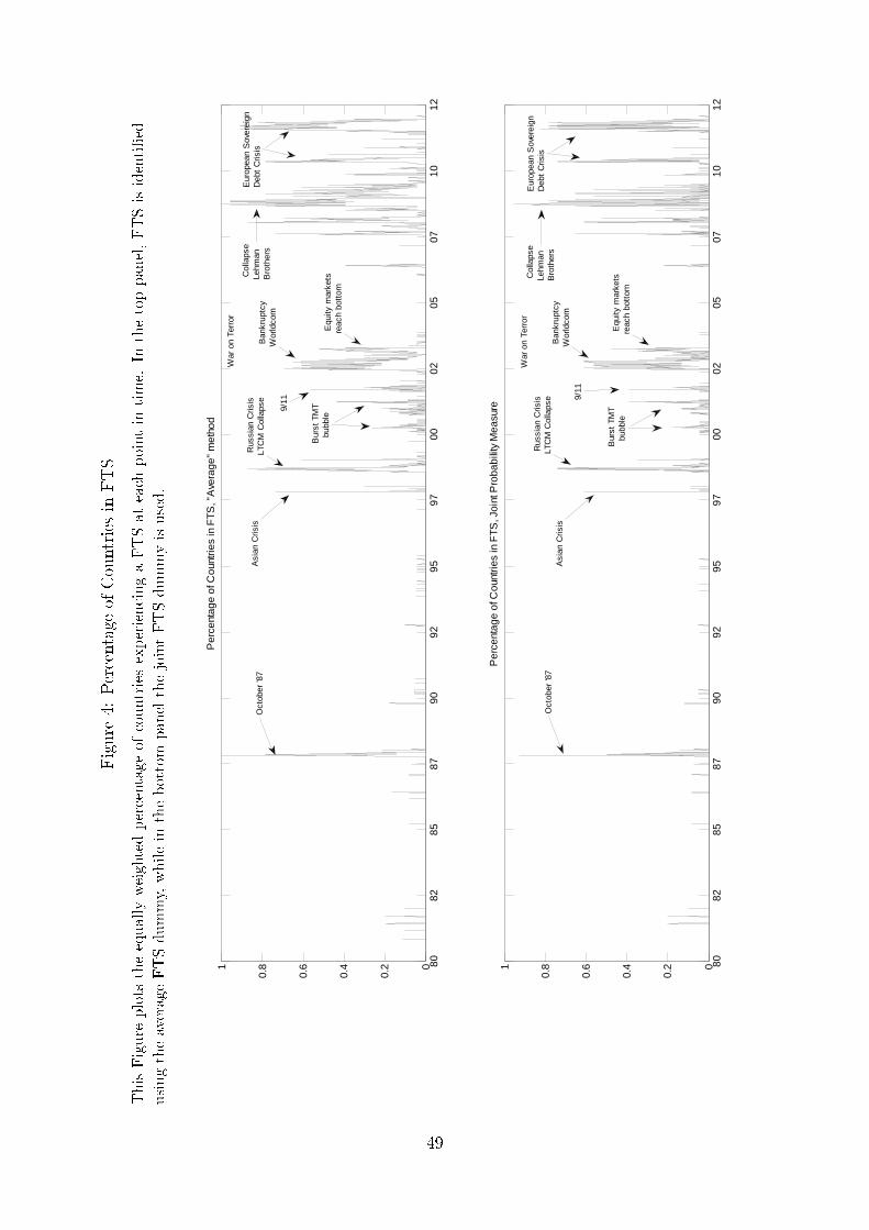
Figure

4:Percentage

ofCountriesin

FTS

ThisFigure

plots

theequally-weightedpercentage

ofcountriesexperiencingaFTSat

each

pointin

time.

Inthetoppanel,FTSisidenti�ed

usingtheaverageFTSdummy,whilein

thebottom

panelthejointFTSdummyisused.

8082

8587

9092

9597

0002

0507

1012

0

0.2

0.4

0.6

0.81

Per

cent

age

of C

ount

ries

in F

TS, "

Ave

rage

" m

etho

d

8082

8587

9092

9597

0002

0507

1012

0

0.2

0.4

0.6

0.81

Per

cent

age

of C

ount

ries

in F

TS, J

oint

Pro

babi

lity

Mea

sure

Oct

ober

'87

Oct

ober

'87

Asi

an C

risis

Asi

an C

risis

Rus

sian

Cris

isLT

CM

Col

laps

e

Rus

sian

Cris

isLT

CM

Col

laps

e

9/11 9/

11

Bur

st T

MT

bubb

le

Bur

st T

MT

bubb

le

Ban

krup

tcy

Wor

ldco

m

Ban

krup

tcy

Wor

ldco

m

Equ

ity m

arke

tsre

ach

bott

om

Equ

ity m

arke

tsre

ach

bott

om

War

on

Terr

or

War

on

Terr

or

Col

laps

eLe

hman

Bro

ther

s

Col

laps

eLe

hman

Bro

ther

s

Eur

opea

n S

over

eign

Deb

t C

risis

Eur

opea

n S

over

eign

Deb

t C

risis

49