life-cycle costing: a guide for selecting energy ... · conservation nbsbuildingscienceseries113...

f. Ill

I AlllDO TTblia

NATL INST OF STANDARDS & TECH R.I.C.

A1 11 009961 12/NBS building science seriesTA435 .use V113;1978 C.I NBS-PUB-C

CONSERVATION

NBS Building Science Series 113

Life-Cyde CostingA Guide for Selecting Energy Conservation Projects

for Public Buildings "

435 \ M• U58 '''•<'»truo«

NO . 113 DEPARTMENT OF COMMERCE • NATIONAL BUREAU OF STANDARDS1978

C.2

NATIONAL BUREAU OF STANDARDS

The National Bureau of Standards' was established by an act of Congress March 3, 1901. The

Bureau's overall goal is to strengthen and advance the Nation's science and technology and

facilitate their effective application for public benefit. To this end, the Bureau conducts

research and provides: (1) a basis for the Nation's physical measurement system, (2) scientific

and technological services for industry and government, (3) a technical basis for equity in

trade, and (4) technical services to promote public safety. The Bureau's technical work is

performed by the National Measurement Laboratory, the National Engineering Laboratory,

and the Institute for Computer Sciences and Technology.

THE NATIONAL MEASUREMENT LABORATORY provides the national system of

physical and chemical and materials measurement; coordinates the system with measurement

systems of other nations and furnishes essential services leading to accurate and uniform

physical and chemical measurement throughout the Nation's scientific community, industry,

and commerce; conducts materials research leading to improved methods of measurement,

standards, and data on the properties of materials needed by industry, commerce, educational

institutions, and Government; provides advisory and research services to other Government

Agencies; develops, produces, and distributes Standard Reference Materials; and provides

calibration services. The Laboratory consists of the following centers:

Absolute Physical Quantities' — Radiation Research — Thermodynamics and

Molecular Science — Analytical Chemistry — Materials Science.

THE NATIONAL ENGINEERING LABORATORY provides technology and technical

services to users in the public and private sectors to address national needs and to solve

national problems in the public interest; conducts research in engineering and applied science

in support of objectives in these efforts; builds and maintains competence in the necessary

disciplines required to carry out this research and technical service; develops engineering data

and measurement capabilities; provides engineering measurement traceability services;

develops test methods and proposes engineering standards and code changes; develops and

proposes new engineering practices; and develops and improves mechanisms to transfer

results of its research to the utlimate user. The Laboratory consists of the following centers:

Applied Mathematics — Electronics and Electrical Engineering^ — Mechanical

Engineering and Process Technology- — Building Technology — Fire Research —Consumer Product Technology — Field Methods.

THE INSTITUTE FOR COMPUTER SCIENCES AND TECHNOLOGY conducts

research and provides scientific and technical services to aid Federal Agencies in the selection,

acquisition, application, and use of computer technology to improve effectiveness and

economy in Government operations in accordance with Public Law 89-306 (40 U.S.C. 759),

relevant Executive Orders, and other directives; carries out this mission by managing the

Federal Information Processing Standards Program, developing Federal ADP standards

guidelines, and managing Federal participation in ADP voluntary standardization activities;

provides scientific and technological advisory services and assistance to Federal Agencies; and

provides the technical foundation for computer-related policies of the Federal Government.

The Institute consists of the following divisions:

Systems and Software — Computer Systems Engineering — Information Technology.

'Headquarters and Laboratories at Gaithersburg, Maryland, unless otherwise noted;

mailing address Washington, D.C. 20234.

•Some divisions within the center are located at Boulder, Colorado, 80303.

The National Bureau of Standards was reorganized, effective April 9, 1978.

NOV 8

NBS Building Science Series 113

A Guide for Selecting Energy Conservation Projects

for Public Buildings

Rosalie T. RueggJohn S. McConnaugheyG. Thomas SavKimberly A. Hockenbery

Building Economics and Regulatory Technology Division

Center for Building Technology

National Engineering Laboratory

National Bureau of Standards

Washington, D.C. 20234

Sponsored by:

Office of Conservation and Solar Applications

Department of Energy


U.S. DEPARTMENT OF COMMERCE, Juanita M. Kreps, Secretary

Dr. Sidney Harman, Under Secretary

Jordan J. Baruch, Assistant Secretary for Science and Technology

NATIONAL BUREAU OF STANDARDS, Ernest Ambler, Director

Issued September 1978

Library of Congress Catalog Card Number: 78-600094

National Bureau of Standards Building Science Series 113Nat. Bur. Stand. (U.S.), Bldg. Sci. Ser. 113, 76 pages (Sept. 1978)

CODEN: BSSNBV

U.S. GOVERNMENT PRINTING OFFICEWASHINGTON: 1978

For sale by the Superintendent of Documents, U.S. Government Printing Office, Washington, D.C.

SD Catalog Stock No. 003-003-01980-1 Price $2.75

PREFACE

This report is addressed primarily to managers and

operators of all types of buildings owned or leased byFederal, State, or local government, including office

bmldings, hospitals, schools, and residential buildings.

It is also applicable to energy conservation investments

in buildings operated by nonprofit, tax-exempt organi-

zations. Because it does not include tax effects, the

report vwll be less useful to the ow^ners, managers, and

operators of privately-owned buildings. However,

aside from the treatment of taxes, the approach is

generally appUcable to the evaluation of energy con-

servation in privately owned buUdings.

The report was prepared by the National Bureau of

Standards and sponsored by the U.S. Department of

Energy. It was developed from Ufe-cycle costing guide-

lines for energy conservation in Federal buildings

prepared by the National Bureau of Standards in

support of the Federal Energy Management Program.

The preparation of guidelines for the Federal Energy

Management Program was required by Executive

Order 12003, "Relating to Energy Policy and Conser-

vation," signed by President Carter on July 20, 1977.

The Executive Order estabUshed goals for Federal

agencies in energy conservation. The goals are to

achieve by 1985, a reduction of 20 percent of the

average annual energy use per gross square foot of

floor area for the total of all Federally ovmed existing

buildings, and a reduction of 45 percent, for the total

of all Federally ovmed new buildings.

The Executive Order further directed Federal agencies

to consider in their building plans only those energy

conservation improvements which are cost effective

based on a Ufe-cycle cost approach, and to give the

highest priority to the most cost effective projects. It

requires that flie determination of cost effectiveness be

consistent with criteria established by U.S. Office of

Management and Budget (0MB) Circular No. A-94,

"Discount Rates to be used in Evaluating Time-

Distributed Costs and Benefits," dated March 27, 1972.

The Executive Order also required that the Department

of Energy provide guidelines to Federal agencies for

estimating Ufe-cycle costs and savings of proposed energy

conservation improvements, and for comparing their cost

effectiveness in a uniform and consistent manner from

agency to agency.

The Ufe-cycle costing guidelines for Federal buUdings —upon which this report is based — contain certain

specific instructions for Federal agencies that are not

necessarily appUcable to the analysis of energy conser-

vation in State and local buildings. In order to broaden

the appUcabiUty of the material for analysis of State

and local government buildings, a distinction is made in

this report between the general requirements of an

economic evaluation and the specific set of economic

criteria that should be foUowed in selecting energy con-

servation projects in Federal buUdings. The report also

indicates to some extent the economic criterion that

appUes to the Department of Energy Grants Program for

Technical Assistance Programs and Energy Conservation

Projects in Schools, Hospitals, Local Government and

PubUc Care Buildings, a program that is exempt from

the requirements of 0MB Circular A-94.

The guidelines for the Federal Energy ManagementProgram and for the Federal Grant Program are, how-

ever, not final at the printing of this report. Therefore,

analysts who need to comply vnth the specific require-

ments of these Federal programs should refer to the

Department of Energy's Program Rules, expected to be

released later this year. Information on the Federal

Energy Management Program and on the Department

of Energy Grants Program for Technical Assistance

Programs and Energy Conservation Projects in Schools,

Hospitals, Local Government and PubUc Care Buildings

can be obtained from the Department of Energy, Office

of Conservation and Solar AppUcations, Washington,

D.C. 20461.

in

ACKNOWLEDGEMENTS

This report was prepared in the AppHed Economics Pro-

gram of the National Bureau of Standards under the

leadership of Rosalie T. Ruegg, with the support of

John S. McConnaughey, G. Thomas Sav, and Kimberly

A. Hockenbery.

The authors which to thank Harold E. Marshall, Chief of

the Apphed Economics Program, Stephen Weber, andPhilhp T. Chen, also of the AppUed Economics Program,

for their valuable comments and assistance. George E.

Turner, Daniel H. Nail, Thomas P. Frazier, and William

G. Hall, aU of the National Bureau of Standards were

helpful in reviewing the draft report.

Appreciation is also extended to the representatives of

an interagency hfe-cycle cost task force, organized by

the Department of Energy, for their advice on the pre-

paration of the guidelines for Federal buildings that

preceded this report. Representatives to the task force

were Michael Walsh, Department of Energy; Virgil

Ostrander, General Services Administration; John

WUUams, Department of the Navy; Frank Durso,

National Aeronautics and Space Administration; Paul

Neal, Department of the Air Force; Lawrence Schind-

ler, Department of Defense; and R.R. Huber and John

Sisty, Veterans Administration.

Special credit is due to John Anderson of the Depart-

ment of Energy who coordinated the Task Force,

oversaw the preparation of the Federal guidelines, and

offered valuable comments on this report.

CONTENTS

1. INTRODUCTION 1

1.1 Background 2

1.2 The LCC Concept: An Overview 2

1 .3 Organization 3

2. BASIC LCC PROCEDURES 5

2.1 Identifying the Alternatives 5

2.2 Time Considerations 6

2.3 Identifying the LCC Parameters 6

2.4 Converting Costs and Savings to a Common Time and Common Dollar Measure 7

2.5 Determining the Most Economical Alternative 1

1

2.6 Sensitivity Analysis 11

3. RANKING ENERGY CONSERVATION PROJECTS FOR EXISTING BUILDINGS 13

3.1 Alternative Ranking Criteria 14

3.2 Calculating the SIR 16

3.2.1 Simple Investment Projects 16

3.2.2 Complex Investment Projects 16

3.3 Calculating the Discounted Payback 27

3.4 Ranking Interdependent Projects 28

3.5 Selecting Projects for Funding 28

4. EVALUATING ENERGY CONSERVATION DESIGNS FOR NEWBUILDINGS 31

5. EVALUATING INVESTMENTS IN SOLAR ENERGY 37

6. DETERMINING ENERGY CONSERVATION REQUIREMENTS FOREXISTING LEASED BUILDINGS 39

7. UNIFORM LCC CRITERIA 41

APPENDIX

A. Glossary of Selected Economic Terms 43

B. Discount Formulas and Factor Tables 45

C. Worksheets for Deriving Economic Ranking Measures for Retrofit Projects

and for Alternative New Building Designs 49

D. Computer Program 59

E. Selected Annotated References 68

V

LIST OF FIGURES AND TABLES

FIGURES

Figure 1 Discounted Payback Nomogram 26

Figure 2 Allocating the Budget Among Alternative Projects Ranked by SIR 29

TABLES

Table 1 Computing the Present Value of Cost and Savings Occurring at Different Times .... 9

Table 2 Worksheet for Calculating the SIR for a Simple Retrofit Project 17

Table 3 Worksheet for Calculating the SIR for a Retrofit Project when Cash

Flows are Complex 19

Table 4 Worksheet for Calculating the Present Value of Energy Savings from a Retrofit

Project when Short-Term and Long-Term Energy Escalation Rates are Used 20

Table 5 Worksheet for Calculating the Net Present Value of Capital Investment Costs

when Costs are Spread Over Time and There is Salvage Value 23

Table 6 Worksheet for Calculating the Present Value of Non-Energy (Maintenance and

Repair) Costs After the Retrofit 25

Table 7 Summary Worksheet for Calculating the Total life-Cycle Costs of the

Energy Components of a New BuUding Project 33

Table 8 Worksheet for Calculating the Present Value of Energy Costs

in a New Building Design 34

Table 9 Worksheet for Calculating the Present Value of Capital Investment Costs

in a New Building Design 35

Table 10 Worksheet for Calculating Non-Energy (Maintenance and Repair) Costs for a

New BuUding Design 36

Table B-1 Discount Formulas 45

Table B-2 Single Present Value Discount Factors for Energy Price

Escalation Rates from 0% to 10% 46

Table B-3 Uniform Present Value Discount Factors for Energy Price

Escalation Rates from 0% to 10% 47

Table B-4 Single Compound Amount Factors for Alternative Interest Rates 48

vi

ABSTRACT

This report provides a step-by-step guide for con-

ducting life-cycle cost evaluations of energy con-

servation projects for public buildings. It explains

the use of life-cycle costing analysis to evaluate

and rank the cost effectiveness of alternative

energy conservation retrofit projects to existing

public buildings, and to select the most cost-effec-

tive design for new buildings. Worksheets,

illustrated with a realistic example, and a computer

program are provided.

This guide is compatible with a life-cycle costing

guide prepared for the Department of Energy for

use in the Federal Energy Management Program

by Federal Agencies. The purpose of this report is

to provide a guide to state and local governments

for use in their energy conservation programs.

Key words: Building economics; economic analysis;

energy conservation; engineering economics;

investment analysis; life-cycle cost analysis.

1 . INTRODUCTION This report has been prepared to assist Federal, State,

and local government officials in evaluating energy con-

servation projects in public buildings, including residen-

tial, commercial, and industrial buildings. It explains the

basic concepts needed to understand the Ufe-cycle

costing (LCC) evaluation method, discusses the choice of

basic assumptions and evaluation criteria, and provides

computational aids in the form of worksheets, a nomo-gram, and a computer program for deriving cost effec-

tiveness measures.

While most other books and reports on life-cycle costing^

describe the general LCC methodology, this report

An annotated list of selected references on life-cycle

1

focuses on the establishment of a technically correct,

practical, standardized approach for evaluating pro-

posed energy conservation improvements in pubUc

bmlding?. Its emphasis is on performing the LCC evalua-

tion of energy conservation investments; it is not intend-

ed as a guide to identifying specific energy conservation

projects, nor a guide to calculating energy consumption.^

Based on the evaluation approach presented here, the

cost effectiveness of alternative projects can be com-

pared in a uniform and consistent manner from agency

to agency. This will assist agencies in selecting and

giving highest priority to those projects which are most

cost effective. (For a definition of economic terms used

in this report, see Appendix A.)

1.1 BACKGROUND

The material from which this report was developed was

prepared in support of the Federal Energy ManagementProgram, as required by Executive Order 12003 [17] . In

order to promote consistency and uniformity amongFederal agencies in their use of LCC analysis for evaluat-

ing energy conservation projects in Federal buildings, the

Executive Order called for the preparation of Federal

guidelines for life-cycle costing. The basic material from

that effort has been broadened here for appUcation to

State and local government buildings. State and local

units of governments, like Federal agencies, require con-

sistent LCC measures to allocate limited funds amongcompeting energy conservation projects and to partici-

pate with other governmental units in State, regional,

and Federal programs for energy conservation. For this

reason, the specific evaluation guidelines that were

developed to promote consistency among Federal

agencies are contained in the following discussion of the

general requirements for performing LCC analysis of

energy conservation projects.

The State Energy Conservation Program, which was

estabUshed by the Energy PoHcy and Conservation Act

(EPCA) of 1975, has been instrumental in stimulating

energy conservation efforts in the States [18] . Over a

three-year period (FY 1976-78), $150 million was

authorized to assist states in developing energy conser-

vation programs. To be eUgible for Federal funds.

States were required to estabUsh certain standards, re-

quirements, and poUcies by January 1978, among which

were

• Ughting efficiency standards for public buildings,

costing is provided in Appendix E. See references [1-7]

.

2 For guidance in identifying potential energy conser-

vation projects for pubUc buildings, in calculating energy

consumption, and in planning and carrying out energy

conservation programs, the reader may consult refer-

ences [8 through 1 6] in Appendix E.

• energy efficiency standards and poUcies to govern

procurement practices, and

• thermal efficiency standards and insulation

requirements for new and renovated buildings.

Virtually every State plan prepared under this program

mentions the use of LCC or some other type of energy/

cost performance criteria to be implemented as part of

EPCA. In addition, these plans indicate a trend toward

development of training programs, seminars, and

workshops to encourage the use of LCC or other pro-

curement techniques suitable for encouraging energy

conservation in products purchased.-^

Many States are utiHzing LCC analysis in conjunction

with their energy conservation programs for pubhcbuildings under state domain. The State of Washington,

for example, is designing an LCC analysis technology

transfer program to provide assistance to local govern-

ments in adopting State energy conservation procedures.

The CaUfomia Energy Commission was mandated bylegislation to develop a life-cycle cost procedure for use

by State agencies and the general pubUc by July 1,

1978 [16].

During its more than 20 years of existence and applica-

tion, hfe-cycle costing has become a generally accepted

means, in both the pubUc and private sectors, of

recognizing the sum total of all costs (and benefits)

associated with a project during its estimated lifetime.

As experience has grown, the apphcation of LCCtechniques has become increasingly sophisticated,

evolving from the use of simple manual calculations to

complex computer programs that require vast data

bases. Many government agencies are currently using

LCC or other economic evaluation techniques, but

differences exist in appUcations and in technical

criteria. Thus, while the LCC technique is not new,

there is a lack of uniformity and consistency in its

use.

In order to facilitate a uniform LCC approach, this

report provides basic ground rules, assumptions, defi-

nitions, and requirements for using the LCC method-

ology. It may be used in conjunction with existing

calculation techniques or models for estimating specific

LCC parameters such as initial investment costs,

future energy costs, or maintenance costs, provided

that these techniques or models satisfy the criteria

included here.

1.2 THE LCC CONCEPT: AN OVERVIEW

LCC analysis is a method of economic evaluation of

alternatives which considers all relevant costs (and

3 Background information on the current regulatory

status and degree of implementation of building energy

conservation projects at the State level are described

in reference [19]

.

2

benefits)^ associated with each alternative activity or

project over its life. As applied to energy conservation

projects in buildings, LCC analysis provides an evalua-

tion of the net effect, over time, of reducing fuel costs

by purchasing, installing, maintaining, operating, re-

pairing, and replacing energy-conserving features.

LCC analysis is primarily suited for the economic com-

parison of alternatives. Its emphasis is on determining

how to allocate a given budget among competing pro-

jects so as to maximize the overall net return from that

budget. The IjCC method is used to select energy con-

servation projects for v/hich budget estimates must be

made; however, the LCC cost estimates are not appro-

priate as budget estimates, because they are expressed

in constant doUars (excluding inflation) and aU dollar

cash flows are converted to a common point in time.

Hence, LCC estimates are not necessarily equivalent to

the obUgated amounts required in the funding years.

The results of LCC analyses are usually expressed in

either present value dollars,^ uniform annual value

4 In evaluating energy conservation investments, it is

important to account for any significant differences in

the benefits of alternatives, such as the effects on the

comfort and productivity of a building's occupants.

5 Expressing LCC estimates in present value doUars

dollars,^ as a ratio of present or annual value dollar

savings to present or annual value dollar costs (referred

to here as the savings-to-investment ratio or SIR), or as

a percentage rate of return on the investment.

Although it is not in a strict sense an LCC measure, the

time until the initial investment is recouped (Payback)

is another form that is sometimes used to report the

results of an LCC analysis. To derive any of these mea-

sures, it is important to adjust for differences in the

timing of expenditures and cost savings. This time ad-

justment can be accomplished by a technique called

"discounting."

The major steps for performing an LCC analysis of

energy conservation investments are the following:

(1) Identify the alternative approaches to achieve

the objective of reducing consumption of non-

renewable energy, as well as any constraints

that must be imposed such as the level of

thermal comfort required.

(2) Estabhsh a common time basis for expressing

LCC values, a study period for the analysis, and

the economic hves of major assets.

(3) Identify and estimate the cost (and benefit)

parameters to be considered in the analysis.

(4) Convert costs and savings occurring at different

times to a common time.

(5) Compare the investment alternatives in terms of

their relative economic efficiencies in order to

select the energy conservation projects that will

result in the largest savings of nonrenewable

energy costs possible for a given budget andconstraints.

(6) Analyze the results for sensitivity to the initial

assumptions.

1.3 ORGANIZATION

A more detailed description of the basic LCC proceduresis given in the following section. The application of LCC

means converting all past and future cash flows associat-

ed with an investment to their equivalent value at the

present time, taking into account the time value of

money, and adding tb.em to first costs, which are al-

ready expressed in present value terms. This process is

explained in Section 2.4.

^Expressing LCC estimates in uniform annual value

dollars means converting all past, present, and future

cash flovi^ to their equivalent value in terms of a series

of level, annual amounts, taking into account the time

value of money; e.g., mortgage loan payments are

usually calculated using the uniform annual value meth-

od, except that the year is generally divided into 12

interest periods. The process of computing annual

value is explained in Section 2.4.

3

procedures to the evaluation of retrofit projects for

energy conservation in existing buildings is described in

Section 3.0. Worksheets, instructions and a sample

problem are provided for calculating the LCC ranking

measure for retrofit projects. The application of LCCprocedures to energy conservation designs for new

buildings is described in Section 4.0, and worksheets

and instructions for evaluating the hfe-cycle costs of

new design alternatives are given. The use of LCC pro-

cedures to evaluate investments in solar energy is

discussed in Section 5.0. The LCC evaluation of con-

servation actions for leased buildings is discussed in

Section 6.0. A summary hsting of selected LCC criteria

to facilitate uniformity in evaluation measures is given

in Section 7.0. Selected economic terms are defined in

Appendix A to encourage consistent usage. Discount

formulas and selected tables of discount factors are

provided in Appendix B for the convenience of the

analyst performing LCC evaluations. A complete set of

blank worksheets for computing LCC measures are pro-

vided in Appendix C. A computer program for perform-

ing the same LCC calculations as provided by the work-

sheets is hsted in Appendix D. An annotated hst of

selected references pertaining to LCC analysis and to

energy conservation is given in Appendix E.

2 . BASIC LCC PROCEDURES 2.1 IDENTIFYING THE ALTERNATIVES

For existing buildings, energy conserving modifications

(retrofits) may be made to the building envelope,

equipment, systems, and components. For example,

alternative retrofits may include adding insulation to

the exterior envelope, replacing existing windows with

more energy conserving window systems, adding a

solar energy system, or upgrading the efficiency of the

existing heating and cooling system. Extensive retro-

fitting may involve complete renovation of the buUding.

In the case of new buildings, it may be possible to use

alternative designs, building sites, and materials to

reduce energy consumption. For example, a building

may be designed for passive utilization of solar energy.

I

In either existing or new buildings, operation and main-

tenance practices may be altered to conserve energy. For

example, an increased frequency of scheduled mainte-

nance may be found to improve the efficiency of equip-

ment and to reduce its energy usage.

2.2 TIME CONSIDERATIONS

To perform LCC analysis, it is necessary to estabUsh a

base time so that all present, past, and future costs can

be converted to a common dollar measure at that base

time. If LCC estimates are to be expressed in present

value dollars, the base time is the present (the time at

which the LCC analysis is being conducted). If LCCestimates are to be expressed in annual value dollars,

the base time is actually a series of time periods of

equal intervals (e.g., years) extending over the period of

the analysis.

An LCC analysis requires the estimation of the economic

life expectancies of the principal assets associated with

each investment alternative. The economic Ufe is that

period over which the asset is expected to be retained in

use as the lowest cost alternative for satisfying its in-

tended purpose. The economic Ufe of the building,

equipment, systems or components is often difficult to

determine. Generally, the facility engineer will deter-

mine hfe based on available technical manuals, infor-

mation from manufacturers and distributors, expecta-

tions for obsolescense, and information of the average

hves of generic types of plants and equipment.^

It is also necessary for the analyst to specify the length

of time, or study period, over which an investment is to

be evaluated. In specifying the study period, it is import-

ant that (1) all mutually exclusive alternatives^ be

evaluated on the basis of the same study period, (2) the

study period not exceed the period of intended use of

the facUity in which the energy conservation investment

is to be made, and (3) if alternatives are evaluated for a

period shorter or longer than the estimated lives of the

principal assets, any significant salvage values or replace-

ment costs should be taken into account.

One of the following four approaches is usually taken

to establish the study period: (1) If it is assumed that

the facility is to be used indefinitely, the study period

can also be assumed to be infinite, and costs can be eval-

uated in armual value dollars based on the economic Ufe

of each alternative investment. For example, the annual

cost of a 10-year hfe investment is calculated on the

basis of 10 years and the annual cost of an alternative

1 5-year Ufe investment is based on 1 5 years. Then it is

^See, for example, reference [3] , pp. B-1 to BA.

^"Mutually exclusive" means that if one alternative

is chosen, the other alternatives wiU not be chosen; e.g.,

if for a given window area, double-glazed windows are

used, triple-glazed windows wiU not be used.

assumed that either would be used indefinitely through

a series of replacements. This approach can in some cases

simpUfy calculations because it eliminates the need to

consider replacements and salvage values. (2) The study

period can be set equal to a period of time that aUows

coincidence of the expiration of alternative investments.

For example, in comparing an investment with a 10-year

Ufe to one with a 15-year Ufe, the study period would be

set equal to 30 years, with three renewals of the first in-

vestment and two renewals of the second. This approach

is often taken to evaluate alternatives over an equal per-

iod of time when results are to be measured in present

value doUars. (3) The study period may be a finite period

of time set to reflect the period of intended use of the

investment or of the faciUty in which the investment is

to be made. (4) Alternatively, the study period may be

set equal to some other finite period to reflect other

constraints, such as the time over which costs andbenefits can be estimated with some degree of accuracy.

Both the third and fourth approaches require the in-

clusion of any relevant replacements or salvage values

when the study period does not coincide with the

expected Uves of the various alternatives. It is also im-

portant in both approaches that mutuaUy exclusive

alternatives to accompUsh a given objective (e.g., solar

screens of type A versus solar screens of type B) be

evaluated for the same finite study period.

It is urmecessary, however, to evaluate retrofit projects

that are not mutuaUy exclusive on the basis of a com-mon study period for purpose of comparing and ranking

them. For example, alternative solar energy systems for

appUcation to Building A may be evaluated over a study

period of, say, 25 years; alternative heat recovery sys-

tems also for BuUding A may be evaluated over a period

of, say, 15 years; and alternative new plant control

systems for Building B may be evaluated over a period

of, say, 10 years. The economic ranking measure for

each of the alternatives selected — each based on its

respective study period — can then be compared with-

out the need to convert aU of the projects to the samestudy period.

Due to uncertainties in forecasting future energy

prices and in order to promote consistency amongagencies, an upper limit of 25 years is imposed onthe study period for analyzing energy conservation

projects in existing buildings in the Federal Energy

Management Program.

2.3 IDENTIFYING THE LCC PARAMETERS

The costs of owning, operating and maintaining an asset

over a period of time are traditionaUy separated into

initial (investment) costs and future (operation, mainte-

nance, repair, and replacement) costs. The investment

costs include aU first costs that arise directly from the

project, including special site-specific studies, design,

and instaUation or construction costs, i.e., all costs

6

necessary to provide the finished project ready for use.

All investment costs should be taken into account in

evaluating alternatives. Sunk costs (that is, costs in-

curred prior to making the LCC analysis) should not be

included. Those costs for studies, analyses, etc., whichare not due directly to a specific project, such as costs

for prehminary energy audits or energy surveys, should

not be included as an investment cost for the purpose of

evaluating a given project.

Future costs can be divided into energy and non-energy

costs. Energy costs are defined here as the dollar cost of

deUvered energy at the building or facility boundary.

Estimates of energy costs are a critical data input to the

LCC evaluation. For an existing building, estimates will

be needed of the building's energy requirements before

it is retrofitted, and projections will be needed of its

expected energy requirements after specific retrofit

actions have been taken.^ For new buildings, it will be

necessary to estimate the expected energy requirements

of alternative building and system designs.

Energy requirements may be estimated at varying levels

of analytical detail, utilizing past records of energy usage,

walk-through surveys of facilities, reviews of specifica-

tions and drawings, engineering test data and computeranalysis of energy flows. Once the impact of a given

energy conservation investment has been estimated,

future doUar energy savings can be projected by first

determining the value of the expected yearly energysavings in today's prices, and then adjusting yearly dollar

savings to reflect expected increases in energy prices

over the study period.

Guidelines for estimating the energy require-

ments of Federal buildings are provided in the

Program Rules of the Federal Energy ManagementProgram. Projections for estimating increases in

energy prices are currently being developed by the

Department of Energy.

Non-energy costs are maintenance, repair, replacement,

and future non-energy operating costs such as operating

personnel costs. For new buildings, where LCC analysis

^For guidance in identifying potential retrofit pro-

jects, see references [8 and 12 through 15] . For guid-

ance in plaiming, managing, and implementing energy

conservation projects and in determining energy re-

quirements, see references [8 through 1 1 and 1 5 and

16].

^°An example of previous projections of energy

prices is the Department of Energy's (DOE) Project

Independence Evaluation System (PIES) [20] . ThePIES projects will be replaced by the new projections

currently in preparation by DOE. PIES projections wiU

not be used either for the Federal Energy ManagementProgram or the Federal Grants Program.

is used to determine the basic building design, future

non-energy costs may also include functional-use costs,

i.e., non-maintenance costs associated with performing

the intended function of the building. For example, the

shape of a building may affect not only its energy re-

quirements, but also its ability to serve its intended

purpose.

The implementation of some energy conservation im-

provements may have Uttle or no effect on maintenance,

repair, or replacement costs (e.g., installing insulation in

the roof of a building). If these costs are not significant-

ly affected, they may be excluded from the analysis.

Where non-energy cost changes are significant, they

should be included in the analysis.

Differences in benefits from alternative investments in

energy conservation should also be taken into account

wherever they are significant. For example, an energy

conserving lighting system may adversely affect the

quahty of Ughting, and, thereby, affect worker pro-

ductivity in a significant way. A comparison of alterna-

tive energy conservation investments based solely on

their energy savings and direct costs is vaHd only if the

investments have no other important consequences.

2.4 CO>rVERTING COSTS AND SAVINGS TO ACOMMON TIME AND COMMON DOLLARMEASURE

The costs and savings associated with investments in

energy conservation are typically spread out over time.

It is necessary to convert costs and savings to a commontime and a common dollar measure to account for the

time value (or opportunity cost) of money. The time

value of money means that there is a difference between

the value of a dollar today and its value at some future

time. The time dependency of value reflects not only

inflation, which may erode the buying power of the

doUar, but also the fact that money currently in hand

can be invested to earn a real return, i.e., it has a real

opportunity cost.

7

Inflation. The adjustment of costs and savings to account

for inflation and for the real opportunity cost of moneycan be accomplished in several ways. If future estimates

of costs and savings include an inflation factor (expected

price changes), it is necessary to remove the inflation

factor so that aU values are expressed in constant dollars.

This is important, because an economic evaluation makes

no sense if it is made in variable-value dollars.

Inflation may be eliminated from the evaluation in any

of three ways: (1) One way is simply to state estimates

of future prices in constant dollars at the outset. This

may be done by assuming that inflationary effects wiU

cancel out, leaving base year prices as good indicators of

future constant dollar prices. Using this approach, any

future prices that are expected to increase differently

from general price inflation must be adjusted to include

the amounts of the expected differential rates of change.

For example, it may be assumed that the price of labor

to perform a given maintenance service will remain at

today's level in constant dollar terms, but that energy

prices will rise above today's level in constant dollars,

i.e., they v^dll increase faster than general price inflation,

say, 3 percent faster for purposes of illustration. Today's

prices for labor could then be used v^dthout adjustment

for the purpose of estimating future maintenance costs,

but today's prices for energy would need to be escalated

at a rate of 3 percent per year for use in measuring

future energy costs. Future amounts that are fixed in

base year dollars, for example, level mortgage payments,

do not inflate vidth other costs and savings. Because they

do not inflate, fixed payments decline in constant dollars

as inflation occurs. To convert fixed amounts in future

years to constant dollars requires the use of a constant

dollar price deflator. If future prices are given in

constant doUars, the real opportunity cost of money can

subsequently be taken into account by using a technique

called "discounting." The technique wiR in this case

employ a real discount rate that also excludes inflation.

(Discounting is explained in more detail below.)

(2) A second way to eliminate inflation, used when the

estimates of future costs and savings are not in constant

dollars, is to apply a constant doUar price deflator to

the estimates of all future costs and savings. "^^ The de-

flator would be applied to fixed, as weU as nonfixed,

future amounts. In this case, the subsequent adjustment

for the real opportunity cost of money is performed as

above, employing a real discount rate (one that excludes

inflation).

(3) A third way of dealing with inflation, also used when

'•''The derivation of a constant doUar price deflator

and its use are demonstrated in reference [21 ] in

Appendix E.

^^Price indices and an explanation of their use can be

found in reference [22] in Appendix E.

the estimates of future cash flows are not in constant

dollars, is to combine the adjustment for inflation with

the adjustment for the real opportunity cost of capital.

This can be done by discounting future costs and savings

stated in current dollars vwth a nominal discount rate,

i.e. a rate that includes both the real opportunity cost

of capital and the expected rate of inflation.

0MB Circular A-94 requires Federal agencies to

express future cash flows in constant dollars, i.e.,

to remove inflation from the estimates of future

costs and savings prior to discounting. Only those

expected price changes over and above the general

inflation rate (i.e., differential change) can be in-

cluded in estimates of future cash flows. This is

the first way of treating inflation listed above. This

is the approach that is to be followed for the Fed-

eral Management Program and the Federal Grants

Program, where differential price changes are

generally allowable only in the case of projecting

future energy prices. It is also the approach to be

followed in the Federal Grants Program, although

the Grants Program is exempt from OMB Circular

A-94.

Discounting. Discounting is performed by applying

interest (discount) formulas, or corresponding discount

factors calculated from the formulas, to the estimated

costs and savings resulting from a given investment. TheappUcation of the appropriate formula or factor to a

cash flow wall convert that cost or saving to its equiva-

lent value at the selected point in time.

The commonly used discount formulas and correspond-

ing tables of discount factors, calculated for specific

time periods and interest (or discount) rates, are pro-

vided in Appendix B. The algebraic equation, notation,

and intended use are given for each formula. The factors

are more convenient to use and give the same results as

the formulas.

The appropriate formula, or factor, to use depends on

the timing of the cost or savings, and on the time basis

selected by the analyst for the economic evaluation. It

is often necessary to use several different discounting

formulas or factors to evaluate a given investment.

Table 1 illustrates the use of four different discount for-

mulas and factors to convert four different types of

costs and savings to a common time. A past cost, a

future recurring cost, a future non-recurring cost, and

future energy savings are all expressed as though they

were to be incurred now. The result obtained is called a

present value.

The Federal Energy Management Program provides

for the conversion of costs and savings to present

values. Although the use of present value is

emphasized in the descriptions and worksheets,

agencies may also use annual values.

Discount Rates. As demonstrated in the examples of

8

X!

01)

saaoU

c u0 ™

1 =

18UQ

hi

Q

uha

SuooIZ!

C>«

s

Ou

M tU O

>-4-1

C(U1/1

-° E

E "

s ia oa.

2

<Q

LL

a

o o

OO

o Ô (N1—I y—t

II II

CO

CP

H >-

CO

00

o.—( 00

II II

<N1

O —IO (N

II II

co

o ^

-5b o•S J

o

to

Oo00

++

CO

p

O

Ph

l-l

V-l

a>Ph

60OoOO

.5 a, r—

1

O O

o >

CD

in C

.5

<1>

3 O

o ^ 2ÎI

pp o^ 'Z

00

oO 00

&oII II

Oh

rn

CQ

II

o

00r-T-H

oo <N

Ph

oo

II

Ph

inin

oo'

00 >II

Ph

o H

•-.Soo ^ Ô M.-H O r;

•Sl-H

tH

o5 «Oh C

_ o

3 O 

+

Z W II

<II

•5 Td c03 -t—> LjC« <l> CU

Td 1-1

O 03

C O

c3

o

Tdo•c

o-ac4H C

3O-a

O <l>

II

9^ >OX)

.S

o

9 § ^-6 o £2 " 3

II f II

< .1 Z

o3 3

II II II

P. H IJh

oZ

c ~

§ &« 2

"!=! C§ Sa O^20 <1J

CO

S E1 2

" 2J pL,

p g(1) s

CQ S

03 u.

CQ W

(-HUh

1^3^% ^

o0 *3

1 cZ .3o ?

oo

9

Table 1 , it is necessary to select a discount rate to per-

form discounting. The purpose of the discount rate is to

reflect the fact that money in hand can commandresources that earn a return; i.e., to reflect the oppor-

tunity cost of money. The discount rate can be selected

to include inflation, in addition to the real opportunity

cost of money (i.e., a nominal discount rate), or it can

be stated exclusive of inflation (i.e., a real discount rate).

In both the pubUc and private sectors, a wide range of

rates are used to discount cash Hows. Discount rates

typically range from rates as low as 2-3 percent to rates

higher than 20 percent. The choice of rates can signifi-

cantly affect the outcome of an evaluation. The higher

the rate, the lower the value of future cash flows.

0MB Circular A-94 requires Federal agencies to

use a real discount rate of 10 percent to evaluate

most Federal investment decisions. The real 10

percent rate is required for the purpose of both

the Federal Management Program and the Federal

Grants Program, although the latter program is

not subject to Circular A-94.

Timing of Cash Flows. To discount, it is also necessary

to make an assumption about the timing of cash flows

within the year of occurrence. In practice, cash flows

usually occur throughout the year, and may not be well

described by any of the following four alternative

assumptions that are usually made to simpUfy the dis-

counting of cash flows; (1) lump-sum, end-of-year cash

flows, (2) lump-sum, beginning-of-year cash flows,

(3) lump-sum, middle-of-year cash flows, and (4) con-

tinuous cash flows throughout the year. However, to

describe the timing of cash flows more accurately would

generally require more effort than is warranted by the

resulting improvement in the economic measures; there-

fore, one of the above four assumptions is usually

adopted.

The discounting factors shown in Appendix B, Tables

B-2 and B-3, can be used to discount cash flows on

either a beginning-of-period or an end-of-period basis bydesignating the initial period as O or as 1 ,

respectively.

The discount factors in the tables can be averaged for

two consecutive periods, or a conversion factor (see

Table B-2) can be used to develop middle-of-period

factors.

^^Some Federal investment decisions are guided byother rates. For example, 0MB Circular A-104 pre-

scribes a real discount rate of 7 percent to analyze Fed-

eral decisions to acquire additional space by building,

renovating, or leasing, when the costs are estimated to

be $500,000 or more. For the purpose of evaluating

energy conservation in new, renovated, or leased

facUities, however. Federal agencies are required to use

a real discount rate of 10 percent.

For consistency in the Federal Energy Manage-

ment Program and the Federal Grants Program,

cash flows should be treated as lump-sum, end-of-

year amounts.

Energy Price Escalation. In escalating future energy

savings, there may be differences in the price escala-

tion of alternative energy sources and in the periods of

time over which various escalation rates are assumed to

prevail. The prices of coal, fuel oil, electricity, and

natural gas are expected to rise at different rates, both

relative to one another and over time. While energy

prices are widely expected to increase faster than

most other prices, it is not clear that very high price

escalation rates will be sustained indefinitely. As

was indicated earher, one approach to dealing with the

increasing uncertainty of energy prices over time in an

economic evaluation is to impose a cut-off time on the

study period. Another approach is to reduce the energy

price escalation rate to zero or to a low level at some

future point in time.

For the purpose of the Federal Energy Manage-

ment Program a distinction is made between the

"short-term" (defined as up to three years from

10

the present) and the "long-term" (defined as the

period beyond three years). For the short-term

period, agencies can use their own escalation rates

as obtained from local power companies, utility

commissions, and their internal analysis, if these

rates are likely to be more accurate than the rates

provided nationwide by DOE. For the long-term

period, agencies should use the escalation rates

provided by DOE in order to provide greater con-

sistency and comparability among agencies' LCCestimates.

2.5 DETERMINING THE MOST ECONOMICALALTERNATIVE

There are several economic evaluation methods that can

be used to determine whether or not a project is cost

effective; that is, whether life-cycle savings equal or

exceed life-cycle costs. Cost effectiveness of an invest-

ment is indicated when any of the following conditions

are met:^^ (1) the total life-cycle costs of the building

is lower with the investment than without it; (2) the net

present value or net annual value of the investment's life-

cycle savings minus life-cycle costs is greater than zero;

(3) the ratio of net life-cycle savings-to-investment cost

is greater than 1 ; (4) the internal rate of return on the

investment is greater than the minimum acceptable rate

of return; (5) the discounted payback period on the

investment is shorter than its expected life.^^

However, economic evaluation methods can be used for

more than simply identifying investments that satisfy a

minimum cost-effectiveness criteron. Greater energy

cost savings per conservation investment dollar spent

can be achieved if: (1) projects are economically optimal

in terms of their design and size, and (2) priority is

given to the most economically efficient projects.

Sizing or determining the economically efficient scale of

an energy conservation project is best accomplished by use

of the total life-cycle cost method, the net present value

of savings method, or the net annual value of savings

method. As long as the total life-cycle costs of a building

decline as the project is increased in scale, or as long as

net life-cycle savings rise, it pays to expand the project.^®

Sizing can also be done by using the savings-to-invest-

ment ratio method or the internal rate of return method,

provided the methods are applied to evaluate each in-

cremental change in an investment, rather than the

total investment.

The Federal Energy Management Program and the

Federal Grants Program do not require the use of

a particular evaluation method for sizing projects.

To give priority to the most economically efficient pro-

jects from among those projects that are identified as

potential candidates, requires a method for ranking pro-

jects. The ranking of retrofit projects is discussed in

Section 3.0, and the ranking of energy conservation

in new building designs is discussed in Section 4.0.

2.6 SENSITIVITY ANALYSIS

Prior to making a final investment decision, it is usually

advisable to evaluate an investment's economic feasibili-

ty based on alternative values of key parameters about

which there is uncertainty, e.g., life, energy price escala-

tion rate, quantity of energy saved, and discount rate.

This can be done by recomputing the LCC measure for

minimum and maximum values of the parameters in

question using a technique called "sensitivity analysis."

The results of a sensitivity analysis enable the decision

maker to consider the consequences associated with

alternative parametric values. By examining the results

together with estimates of the likelihood of the various

values occurring, the decision maker is better able to

decide if an investment should be undertaken.

0MB Circular A-94, which applies to the Federal

Energy Management Program, but not to the

Federal Grants Program, requires Federal agencies

to conduct sensitivity analysis of proposed pro-

grams and projects, provided that there is a

"reasonable basis to estimate the variability of

future costs and benefits." It is further specifically

required that the prescribed 1 0 percent discount

rate be used to evaluate all alternatives and that

different discount rates should not be used to re-

flect the relative uncertainty of alternatives.

^^The economic evaluation methods for deriving

these results are defined in the Glossary, Appendix A.

^^The payback is a reliable indicator of cost effec-

tiveness only if it is calculated on the basis of discounted

costs and savings and if there are no costs of sufficient

magnitude after the point of payback to affect subse-

quent savings.

Although this condition holds in theory only whenthere are no limitations on the budget, it is generally

followed in practice whether there is or is not a budget

constraint, because of the difficulty of simultaneously

equating the marginal return on all energy conservation

projects. With a budget constraint, the most economi-

cally efficient size of an energy conservation project is

that size for which the ratio of savings to costs for the

last increment in the investment is just equal to the

ratio for the last increment on the next best available

investment. For methods of finding the most efficient

sizes of energy conservation projects with and without

budget constraints, see reference [23] which treats

the optimal level of insulation, and reference [24] which

treats the optimal sizing of solar collectors.

11

3. RANKING ENERGYCONSERVATION PROJECTSFOR EXISTING BUILDINGS

A method is needed for selecting and giving highest pri-

ority to those retrofit projects in existing buildings

which are most cost effective. With a Umited budget for

energy conservation projects, selection of projects on

the basis of their comparative cost effectiveness will

mean more savings per investment dollar. Ranking

projects within an organization will help to ensure the

economic efficiency of its expenditures, and ranking

projects across groups of participating organizations

will contribute to the overall goal of maximum savings

for a given total budget.

13

3.1 ALTERNATIVE RANKING CRITERIA

There are a number of criteria that might be considered

in evaluating the relative cost effectiveness of energy con-

servation projects for retrofitting existing buildings.

Some possible criteria are the savings-to-investment

ratio, the internal rate of return on investment, the net

present value (or net annual value) of the investment,

and the discounted payback period. Another possible

criterion is the quantity of energy saved per investment

dollar spent, e.g., the annual Btu savings per investment

doUar, or some variation of this measure, such as the

armual Btu savings per average investment doUar or the

annual Btu savings per annuaHzed investment dollar.

The following is a brief assessment and comparison of

these alternative criteria that might be considered for

ranking competing retrofit projects.

The Savings-to-Investment (SIR) Ratio as a Ranking

Criterion. The Savings-to-Investment (SIR) Ratio is de-

fined as the ratio of the net present value of savings to

the present value of investment costs. The SIR provides a

technically correct ranking criterion that meets the eco-

nomic efficiency objective of saving the most energy

doUars for a given energy conservation budget. It incorp-

ates all present and future dollar savings and costs over

the Hfe of the project, including those from energy

sources and non-energy sources such as labor and

materials.

Selecting projects in descending order of their SIR's

until the available budget is exhausted wiU result

in the largest total doUar savings for a given budget. Bytreating energy savings in monetary terms, the SIR mea-

sure recognizes present and future differences in energy

savings and costs from alternative sources of energy

(e.g., fuel on, electricity), as well as from regional varia-

tions in energy costs. For example, the SIR would re-

flect that a reduction in energy usage of a million Btu's

of fuel oil may save $3.00, whereas a reduction of a

milhon Btu's of electricity may save $8.00. Similarly,

the SIR would reflect that electricity may cost $.06 per

kilowatt hour in one region of the country and $.03 in

another region.

Since it is based on dollar values, the SIR does not dis-

tinguish between doUar savings occurring from energy

sources and dollar savings occurring from non-energy

sources such as labor or materials. On the one hand, this

feature may require the need for supplementary project

selection criteria to ensure that an energy conservation

program is indeed supporting energy conservation pro-

jects. On the other hand, it is important that significant

non-energy savings be taken into account.

The Internal-Rate of Return (IRR) as a Ranking

Criterion. The IRR method calculates the rate of return

which an investment is expected to yield. The IRR is

generally equivalent in technical accuracy to the SIR for

ranking retrofit projects. like the SIR, the IRR incor-

porates all present and future energy and non-energy

dollar savings and costs over the project Ufe. For situa-

tions in which the minimum acceptable rate of return of

the organization is subject to change, the IRR methodoffers an advantage over the SIR. Because the SIR is

computed using a particular discount rate, it would be

necessary to recompute it if the appUcable discount

rate changed. In contrast, the IRR solves for the rate that

equates costs and savings, and this rate can then be com-

pared with the current discount rate. Because the 10

percent discount rate prescribed by 0MB is not expected

to change in the near future, this difference in the twomethods does not appear relevant to the evaluation of

Federal projects. The IRR has the disadvantage of often

being more cumbersome to calculate than the SIR.^^

The Net Present Value Savings (NPV) as a Ranking

Criterion. The NPV indicates whether a project wiU

save more than it costs and is a particularly useful

method for sizing a project; however, it does not serve

weU as a criterion for ranking projects within a limited

budget. It does not distinguish, for example, between

a large project that saves a given dollar amount of energy

and a smaller project that results in the same dollar

savings. Ranking projects in descending order of their

net present value savings until the budget is exhausted

wiU not guarantee the largest dollar savings per conser-

vation budget.

The Discounted Payback as a Ranking Criterion. The

discounted payback method evaluates energy and non-

energy savings and costs in common dollar terms, but

does not incorporate all relevant costs and savings in the

measure. It thereby results in a partial measure of econo-

mic efficiency. A project with a shorter payback mayyield lower net benefits than a project with a longer pay-

back. Therefore, ranking projects in ascending order of

their payback periods wiH not necessarily result in the

largest dollar savings per investment dollar spent; it wiU

favor the selection of short-lived projects. In some cases

of uncertainty, or when there is a need to recover invest-

ment funds quickly, this feature may be deemed desir-

able. The payback method has the advantages of being

an easy to understand concept and a method which

many organizations are experienced in using. But whenproperly expressed in discounted terms, it offers no

particular computational advantage over the other

methods.

Btu per Investment Dollar as a Ranking Criterion. The

Btu criterion gives weight to the armual quantity of

energy saved, but does not take into account the rela-

tive scarcities of different types of energy, as reflected

^' For a description of the computation of the IRR,

see reference [1]

.

^^The discussion of net present value as a ranking

criterion would apply also to the net annual value sav-

ings method and the total-life-cycle cost method.

14

by their present prices or as can be accounted for byapplying escalation rates; nor does it account for the

expected Hfe of the project or for the time value ofmoney. Relating annual Btu savings to investment costs

also neglects non-energy savings and costs.

This measure, used as a ranking criterion, cannot berehed upon to yield the largest dollar savings for a given

conservation budget. In the short run, it will yield the

largest Btu energy savings (if based on energy consump-tion at the source). However, it may not yield the

largest Btu savings in the long run, because dollar

savings foregone in the short run will not be available

to purchase more energy conservation investments.

Selecting Ranking Criteria: Conclusion. AH the measures

except the last listed above provide for the evaluation

and comparison of both investment costs and the result-

ing savings in economic terms, although the measures

are not all equally effective as ranking criteria. The last

measure listed (Btu criterion) allows for only the invest-

ment costs to be evaluated in economic terms, while thesavings are evaluated in terms of quantity of energy, withno measure of economic value attached to that quanti-

ty. The appeal of the latter type of measure is that bystating savings in terms of units of energy, the measure

appears to focus more directly on the essence of an

energy conservation program, i.e., saving energy. How-ever, by failing to attach economic values to the savings,

this type of measure fails to give priority to the mosteconomically efficient projects.

If the objective of an energy conservation program is

to reduce energy consumption in the most cost-effective

way, either the savings-to-investment ratio method or the

internal rate of return method is the most suitable cri-

terion for ranking and selecting retrofit projects. Bothmethods provide a measure of the return on the doUar

spent, and will result in a selection of projects that wiUyield the largest dollar savings for a given budget. In

contrast, ranking projects in order of their net present

values (or net aimual values), their payback periods, or

their ratios of quantity of energy saved to investment

cost, cannot be reUed upon to obtain the largest savings

for a given budget.

However, the discounted payback method may be a use-

ful ranking criterion in certain cases where uncertainty

is great or where there is a particular need to recover in-

vestment funds quickly. Also, a measure of the quantity

of energy saved in relation to the cost incurred may be a

useful measure for distinguishing between projects that

"•^In considering the Btu measure for ranking pro-

jects, it would, therefore, be necessary to pre-screen the

projects using some other measure in order to ensure

that life-cycle savings exceed life-cycle costs and that

the minimum cost-effectiveness criterion is met.

save energy and those that save non-energy doUars, if

this is important to the energy conservation program.

But due to the significant economic inefficiencies that

can result from sole reliance on either of three measures,

they are not recommended as primary ranking devices.

They may be helpful as supplements to either the savings-

to-investment ratio or the internal rate of return method.


ment Program, the savings-to-investment ratio

method is required for ranking retrofit projects to

determine funding priorities. The Btu and dis-

counted payback measures are secondary criteria

which are recommended for choosing between

projects having identical SIR's. The Federal Grant

Program, on the other hand, has several ranking

criteria, the discounted payback method being one

of the primary criteria.

For new buildings , where all energy-related cash

flows are usually stated as costs, and the objective

is to achieve the lowest overall total cost for the

energy-related components of the building, the

Federal Energy Management Program requires that

the various costs be stated in present values and

summed to derive the total life-cycle cost (TLCC).

For a given building, priority is to be given to the

design with the lowest TLCC, that meets the

15

functional requirements of the building and other

constraints.20

In the Section that follows, the SIR and the discounted

payback methods are described in more detail. The

calculation of both methods is explained, and compu-

tational aids are provided in the form of worksheets

and a nomogram. The net present value method is

described in Section 4.

3.2 CALCULATING THE SIR

The basic step-by-step procedure for calculating the SIR

is as follows: (1) Compute the denominator of the SIR

by finding the net present value of investment costs.

(2) Compute the present value of future energy savings,

where energy savings are defined as the difference be-

tween the cost of energy in the existing building situa-

tion and the expected cost of energy if the energy con-

servation investment were made. (3) Determine if the

investment is expected to raise or lower future non-

energy costs such as maintenance and repair, and com-

pute the present value of the change.^ (4) Compute the

net present value of cost savings, the numerator of the

SIR, by subtracting from (adding to) the present value

of energy cost savings (Step 2), the increase (the de-

crease) in non-energy costs (Step 3). (5) Compute the

SIR by dividing the present value of savings net of

future non-energy costs (Step 4) by the net present

value of project investment costs (Step 1).

This procedure can be performed manually using the

worksheets provided in Appendix C (C-1 or C-2) and ex-

plained and illustrated below, or it can be performed

using the computer program described in Appendix D.

3.2.1 Simple Investment Projects

Energy conservation projects are easy to evaluate if they

(1) require a lump-sum initial investment, (2) are expect-

ed to result in a level quantity of yearly energy savings

with a steadily escalating price, (3) do not significantly

20The TLCC should reflect any differences in the

expected benefits of alternative designs.

2^ This instruction is based on the assumption that

the retrofit project does not affect significantly the

functional use or performance of the building. If it is

expected to have a significant impact on the building,

other than on its energy requirements, the positive or

negative impacts on productivity or on other aspects

of using the building should be assessed, and either

quantitative measures should be developed for incorpor-

ation into the numerator of the SIR or qualitative mea-sures should be developed for consideration.

affect non-energy costs or benefits, and (4) have nosignificant salvage value at the end of the study period.

The SIR for this type of project is simple to compute

because there are no future non-energy costs or benefits

to calculate, and the initial investment is already in pre-

sent value terms. To compute the SIR in this case, it is

necessary only to multiply the initial annual energy

savings by the appropriate present value factor and to

divide this product by the initial investment cost.

Table 2 illustrates with a sample problem the worksheet

approach to evaluating the LCC of a simple investment

project. (A blank copy of the worksheet, numberedC-1 , is provided in Appendix C.) The sample investment

problem is for a simple retrofit project to add insulation

to buildings. For the purpose of this example, a 6 per-

cent differential rate of escalation in energy prices is

assumed. (The uniform present worth factor is taken

from Table B-3, 6% Collumn, year 25.)

Items 1 through 7 of the worksheet provide information

about the nature of the project, its location, and expect-

ed duration. Item 8 gives the investment cost. Item 9, Athrough F, tabulates the information required to com-

pute the annual energy savings. Item 9A gives the annual

quantity of energy saved, measured in units purchased

at the building boundary. The annual quantity saved is

then multiplied by Item 9B, the current price per unit

of energy, to obtain Item 9C, the initial value of annual

energy savings. Item 9D identifies the expected rate of

energy price escalation. Item 9E, the uniform present

worth factor (obtained from Table B-3) is multiplied byItem 9C to calculate Item 9F, the present value of sav-

ings. Item 10 gives the sum of entries in Item 9F. TheSIR, Item 11 , is calculated by dividing Item 10, the

total present value of energy savings, by Item 8, the pro-

ject investment cost.

Alternatively, to use the computer program (Appendix

D) to calculate the SIR, it is necessary to enter the basic

data from Items 1 through 9 of Table 1 , into the com-puter. The computer then calculates the present value of

the energy savings and divides this value by the invest-

ment cost to obtain the SIR.

3.2.2 Complex Investment Projects

Any of the following conditions mean a more complexinvestment project for which the worksheet in Table 2

may be inadequate:

(1) The proposed project may be expected to change

future non-energy costs or benefits significantly.

(2) Investment costs (planning, design, and

construction) may stretch significantly beyond

the base year of the LCC analysis.

(3) The projected rate of price escalation for each

type of energy may change in the future.

If any of these conditions exist, the calculation of the

SIR requires more computations than are allowed for in

16

TABLE 2

Worksheet for Gilculating the SIR for ;i Simple Retrofit F'roject*

1 . Name of AgencyNational Administration

Install Insulation2. Project Description

3. LocationSuburban Washington, D.C.

4. Gross Floor Area Affected140,000 square feet

5. Expected Life of Project

8. Project Investment Cost

(Date 1 July 1978)

40 years

6. Expected Lite of Buildmg ^^^^^

7. Study Period ^5 years

$41,000

9. Value of Annual Energy Savings

(A)

Units of

EnergySaved at

BIdg/Facility

Boundary

(B)

Current UnitEnergy Price

(Date 7 1 78

(C)

Initial AnnualEnergy Savings

(Date 7 '1 '78)

(C)=(A)x(B)

(D)

EnergyEscalation

Rate

(E)

Uniform Present

Value Factor for

Specified EnergyPrice Escalation

Rate

fF)

Present

Value

(Date 7/1/78)

(F)=(C)x(E)

606060 kWh

Electricit>-

therms

Natural Gas

eal.

Fuel Oil

033

S Per kWli

S Per Therm

S Per Gal.

520,000 6% 16.0026 $320,052

Other S Per.

10. Total Savings$320,052

11. SIR (Item 10 ~ item 8)7.81

*This is Appendix Worksheet C-1.

17

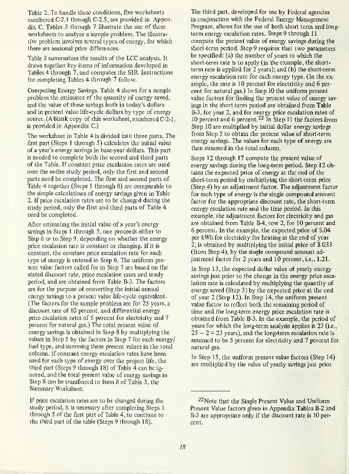
Table 2. To handle these conditions, five worksheets

numbered C-2.1 through C-2.5, are provided in Appen-

dix C. Tables 3 through 7 illustrate the use of these

worksheets to analyze a sample problem. The illustra-

tive problem involves several types of energy, for which

there are seasonal price differences.

Table 3 summarizes the results of the LCC analysis. It

draws together key items of information developed in

Tables 4 through 7, and computes the SIR. Instructions

for completing Tables 4 through 7 follow.

Computing Energy Savings. Table 4 shows for a sample

problem the estimates of the quantity of energy saved,

and the value of these savings both in today's dollars

and in present value life-cycle dollars by type of energy

source. (A blank copy of this worksheet, numbered C-2-1

,

is provided in Appendix C.)

The worksheet in Table 4 is divided into three parts. The

first part (Steps 1 through 5) calculates the initial value

of a year's energy savings in base-year dollars. This part

is needed to complete both the second and third parts

of the Table. If constant price escalation rates are used

over the entire study period, only the first and second

parts need be completed. The first and second parts of

Table 4 together (Steps 1 through 8) are comparable to

the simple calculations of energy savings given in Table

2. If price escalation rates are to be changed during the

study period, only the first and third parts of Table 4

need be completed.

After estimating the initial value of a year's energy

saving in Steps 1 through 5, one proceeds either to

Step 6 or to Step 9, depending on whether the energy

price escalation rate is constant or changing. If it is

constant, the constant price escalation rate for each

type of energy is entered in Step 6. The uniform pre-

sent value factors called for in Step 7 are based on the

stated discount rate, price escalation rates and study

period, and are obtained from Table B-3. The factors

are for the purpose of converting the initial annual

energy savings to a present value Ufe-cycle equivalent.

(The factors for the sample problem are for 25 years, a

discount rate of 10 percent, and differential energy

price escalation rates of 5 percent for electricity and 7

percent for natural gas.) The total present value of

energy savings is obtained in Step 8 by multiplying the

values in Step 5 by the factors in Step 7 for each energy/

fuel type, and summing these present values in the total

column. If constant energy escalation rates have beenused for each type of energy over the project Ufe, the

third part (Steps 9 through 1 8) of Table 4 can be ig-

nored, and the total present value of energy savings in

Step 8 can be transferred to Item 8 of Table 3, the

Summary Worksheet.

If price escalation rates are to be changed during the

study period, it is necessary after completing Steps 1

through 5 of the first part of Table 4, to continue to

the third part of the table (Steps 9 through 18).

The third part, developed for use by Federal agencies

in conjunction with the Federal Energy ManagementProgram, allows for the use of both short term and long-

term energy escalation rates. Steps 9 through 1

1

compute the present value of energy savings during the

short-term period. Step 9 requires that two parameters

be specified: (a) the number of years to which the

short-term rate is to apply (in the example, the short-

term rate is appUed for 2 years); and (b) the short-term

energy escalation rate for each energy type. (In the ex-

ample, the rate is 10 percent for electricity and 6 per-

cent for natural gas.) In Step 10 the uniform present

value factors for finding the present value of energy sav-

ings in the short-term period are obtained from Table

B-3, for year 2, and for energy price escalation rates of

10 percent and 6 percent. In Step 11 the factors from

Step 10 are multiphed by initial dollar energy savings

from Step 5 to obtain the present value of short-term

energy savings. The values for each type of energy are

then summed in the total column.

Steps 1 2 through 1 7 compute the present value of

energy savings during the long-term period. Step 12 ob-

tains the expected price of energy at the end of the

short-term period by multiplying the short-term price

(Step 4) by an adjustment factor. The adjustment factor

for each type of energy is the single compound amount

factor for the appropriate discount rate, the short-term

energy escalation rate and the time period. In this

example, the adjustment factors for electricity and gas

are obtained from Table B-4, row 2, for 10 percent and

6 percent. In the example, the expected price of $.04

per kWh for electricity for heating at the end of year

2, is obtained by multiplying the initial price of $.033

(from Step 4), by the single compound amount ad-

justment factor for 2 years and 10 percent, i.e., 1.21.

In Step 13, the expected dollar value of yearly energy

savings just prior to the change in the energy price esca-

lation rate is calculated by multiplying the quantity of

energy saved (Step 3) by the expected price at the end

of year 2 (Step 12). In Step 14, the uniform present

value factor to reflect both the remaining period of

time and the long-term energy price escalation rate is

obtained from Table B-3. In the example, the period of

years for which the long-term analysis appHes is 23 (i.e.,

25 — 2 = 23 years), and the long-term escalation rate is

assumed to be 5 percent for electricity and 7 percent for

natural gas.

In Step 15, the uniform present value factors (Step 14)

are multiphed by the value of yearly savings just prior

22Note that the Single Present Value and Uniform

Present Value factors given in Appendix Tables B-2 and

B-3 are appropriate only if the discount rate is 10 per-

cent.

18

TABLE 3

Worksheet for Calculating the SIR for a Retrofit Project when Cash Flows are Complex*

(Project Summary Sheet)

1. Name of Agency National Administration

Installation of a Central Automatic Environmental

2. Project DescriptionControl System to serve the Entire Building Facility

3 LocationSuburban Washington, D.C.

4. Gross Hoor Area Affected 2.3 million square feet

5. Expected Ufe of System "^^^^^

6. Expected Life of BuUding V^^''^

7. Study Period ^^^^^

$22,774,758

ENERGY SAVINGS

8. Total Present Value of Energy Savings

(Item 18, Table 4)

INVESTMENT COST

9. Present Value of Investment Cost Less Salvage.

$1 ,384,91 5

(Item 9, Table 5)

NON-ENERGY COSTS (or SAVINGS)

10. Present Value of Non-Energy Costs for the Retrofitted Building$739,836

(Item 10, Table 6)

11 . Present Value of Non-Energy Costs for Existing Building or System(Worksheet C-2.5)

12. Present Value of Change in Non-Energy Costs $739,836

(Line 10 minus Line 1 1 , or (difference method) Line 10)

SIR NUMERATOR

$i99 034 Q??13. Total Present Value of Energy Savings Minus Non-Energy Costs ^ '

'

(Line 8 minus Line 12)

UFE-CYCLE COST MEASURES

14. SIR 15.91

(Line 13 ^ line 9)

15. Net Savings in Present Value $20,650,007

(Line 13 — Line 9)

*This is Appendix Worksheet C-2.1.

NA = Not Applicable

19

TABLE 4

Worksheet for Calculating the Present Value of Energy Savings from a Retrofit Project

when Short-Term and Long-Term Energy Escalation Rates are Used*

:alculatiqn of base year energy costs

(1) Annual Consumption, Existing System

(2) Annual Consumption. Proposed AHemative

(3) Annual Quantity Saved(3) = in-(3)

(4) Today's Local Price/Unil

(5) Today's Annual S Savings (5) = (3) x (4)

71,489.000 kWli

66.500,000 kWh

4.980.000 kWh$.033/kWh

$164,340

CoolingI

28.330.000 kWh25,400,000 kWh"

2,930.000 kWh$.038/kWh

$m.340

43,360.000Tlierms

38,680.000Therms

4,680.000Therms

S.225/ThGrfi.

$1 ,053.000

CONSTANT PRICE ESCALATION ADJUSTMENT

(6) Constant Price Escalation Rale

(7) Unifotm Present Value Factor'*

(8) Present Value Energy Savings (8) = (S) x (7)

14.4367

$1,607,382

17.7998

$18,743,189

SHORT-TERM/LONGTERM PRICE ESCALATION ADJUSTMENT

C?) Expected Real Short-Term Price Escalation

from End of Year 0 lo End of Year _ 2( 10) Uniform Present Value Factor for Short-

Term Price Escalation

(11) Present Value of Short-Term Energy

Savings (II )= (5) X (10)

(12) Expected Price End of Year

(See Instructions)

( 13) Value of Annual Saving in Year 3

(I3) = (3)x(12)

(14) Uniform Present Value Factor for Long-

Term (See Instructions)

(15) Discounted Value of Savings in Year 3

(15) = (13) X (14)

(16) Single Present Value Factor

(See Instructions)

(17) Piesent Value of Long-Term Energy Savinp

(17) = (lS)x(16)

(18) Present Value of Total Energy Savings

(18) = (11) + (17)

2.0

$222,680

$.046

$134,780

13.7968

$1,859,533

.8264

SI .536.71

8

$1,759,398

6%

1.8921

$1,992,381

S-253

$1,184,040

16,7841

$19,873,046

.8264

$16,423,085

$18,415,466

•This is Appendix Worksheet C-2.2.

"Sample problem based on the assumption of a discount rate of 10 percent and a study period of 25 years.

20

to the change in escalation rates (Step 13), to obtain

the value of energy savings over the remaining years,

discounted back to the year the escalation rate changed.

In the example, the factors are multiphcd by the value

of savings in the third year to obtain the value of

savings over the remaining 23 years discounted to the

third year. In Step 16, the single present value factor

for converting total savings from the year the escalation

rate changed to the base year is obtained from Table

B-2. In the example, the factor of .8264 is obtained

from Table B-2, row 2. column 0 percent.

In Step 17. the value of savings over the long-term are

converted back to the base year by multiplying the

single present value factor (Step 16) by the discounted

value of savings in the tliird year (Step 15). The long-

term energy savings are summed across the different

energy types and given in the total column for Step 1 7.

Finally, in Step 18, the short-term energy savings (Step

II ) and the long-term energy savings (Step 17) are

summed. The total savings from Item 1 8 are entered

as Item 8 on the Worksheet in Table 3 if both short-

term and long-term energy escalation rates are used.

21

Computing the Net Present Value of Investment Costs.

Table 5 demonstrates the use of the worksheet for com-

puting the net present value of investment costs whenthe investment occurs in more than one year, when there

are substantial replacement costs, and/or when a signifi-

cant residual or salvage value is expected to remain at

the end of the study period. Investment costs in the base

year are already in present value terms. Thus, for the

sample problem, the $725,000 incurred in the base year

(year 0, column 2) is entered unchanged in the present

value column (year 0, column 6). Investment in subse-

quent years must be discounted to a present value using

single present value factors from Table B-2. For the

sample problem, the $725,000 incurred at the end of

the first year is discounted to an equivalent value of

$659,100 in column 6 by applying the single present

value factor of .9091 (from Table B-2, year 1 , 0 per-

cent escalation). In the sample problem an additional

major replacement investment in year 10 is made of

$50,000, which is discounted to an equivalent value of

$19,275 in column 6 by applying the single present

value factor of .3855 from Table B-2, year 10, 0 per-

cent escalation. The residual or salvage value (column

3) is the net sum which could be expected to be

reahzed from disposal of the investment at the end of

the study period. For the sample problem, the estimate

of $200,000 of residual value evaluated in constant

doUars is placed in column 3 in the final year of the

study period. The $200,000 residual value is discounted

to a present value of $18,460 (column 5) by use of the

single present value factor of .0923 (from Table B-2, year

25, 0 percent escalation).

The net present value of investment costs (Item 9) is

then obtained by summing the present values of invest-

ments in column 6 and subtracting the present value of

the residual in column 5. The net present value of

investment costs ($1,384,915) is entered as Item 9 on

the worksheet in Table 3.

Alternatively, replacement costs and salvage values

could be combined in the numerator with, other future

cash flows, rather than combined with investment costs

in the denominator as provided in Table 5. While this

change in the method of computing the SIR will change

its numerical value, it often wiU not change the relative

order of ranking projects. However, under conditions

where projects with large salvage values and/or replace-

ment costs are being compared with projects with Httle

or no salvage and/or placement costs, it is possible for

the relative ranking of projects also to be changed

sUghtly. If the objective is the largest return on the pre-

sent year's investment dollars, future investment costs

will usually be put in the numerator. If the objective is

the largest return on the long-run budget, future invest-

ment costs wiU usually be put in the denominator. If

the SIR is greater than 1 , having subtracted future

investment costs from the numerator, other things

equal, would have resulted in a higher SIR than having

added these costs to the denominator. Thus a project

with significant future investment costs will look better

relative to a project without significant future invest-

ment costs if the future costs for the first project are

put into the numerator of the SIR. Placing the present

value of future investment costs in the denominator

of the SIR gives as much weight to these costs as to

the initial investment costs.


ment Program, future investment costs are put in

the denominator of the SIR.

22

TABLE 5

Worksheet for Calculating the Net Present Value of Capital Investment Costswhen Costs are Spread Over Time and There is Salvage Value*

Year

(1)

0

1

3

4

5

Investment Costin Constant $(Planning, Design,

Construction,

Replacement)

(2)

$725,000

725,000

Salvage

Value at End of

Study Periodin Constant $

(3)

Single Present

Value Factor for

Year Indicated

(from Table B-1)

(4)

1.0

.9091

.8264

.7513

Present Valueof Salvage

(5)=(3)x(4)

Present Valueof Investment for

Year Indicated

(6H2)x(4)

$725,000

659,100

10 50,000 .3855 19,275

25 $200,000 .0923 $18,460

Totals$18,460 $1,403,375

(7) Present Value of Investment Costs, (Sum of Column 6):

(8) (minus) Present Value of Salvage Value (Sum of Column 5):

(9) (equals) Net Present Value of Investment Costs:

$1,403,375

$18,460

$1,384,915

*This is Appendix Worksheet C-2.3

23

TABLE 3

Worksheet for Calculating tlie SIR for a Retrofit Project when Cash Flows are Complex*

(Project Summary Sheet)

National Administratic

Project Description

I . Name of Agency _

Installation of a Central Automatic Environmental

Control System to serve the Entire Building Facility

Suburban Washington, O.C.3. Location

4. Gross Roor Area Affected 2.3 million square feet

5. Expected Life of Svsiem"^^^^^

6. Expected Life of Building .

7. Study Period

30 years

ENERGY SAVINGS

INVESTMENT COST


SIR NUMERATOR

! 3, Total Present Value of Energy Savins Minus Non-Enerey Costs$22.034,922

(Line 8 minus Line 12)

UFE-CYCLE COST MEASURES


NA - Not Applicable

19

Computing the Net Preseni Value of Investment Costs.

Tabic S demonstrates the use of the worksheet for com-puting the net present value of investment costs whenthe investment occurs in more than one year, when there

are substantial replacement costs, and/or when a signifi-

cant residua] or salvage value is expected to remain at

the end of the study period. Investment costs in the base

year arc already in present value terms. Thus, for the

sample problem, the S725.000 incurred in tlie base year

(year 0. column 2) is entered unchanged in the present

value column (year 0. column 6). Investment in subse-

quent years must be discounted to a present value usmgsingle present value factors from Table B-2. For the

sample problem, the S725,000 incurred at the end ofthe first year is discounted to an equivalent value of

3659,100 in colurrm 6 by applying the single present

value factor of .9091 (from Table B-2, year 1 . 0 per-

cent escalation). In the sample problem an additional

major replacement investment in year 10 is made ofSSO.OOO, which is discounted to an equivalent value of

519,275 in column 6 by applying the single present

value factor of .3855 from Table B-2, year 10. 0 per-

cent escalation. The residual or salvage value (column3) is the net sum which could be expected to be

reaUzed from disposal of the investment at the end ofthe study period. For Ihe sample problem, the estimate

of 3200,000 of residual value evaluated in constant

dollars is placed in column 3 in the final year of the

study period. The $200,000 residual value is discountedto a present value of 518,4(30 (colunm 5) by use of thesingle present value factor of .0923 (from Table B-2, year

25, 0 percent escalation).

The net present value of investment costs (Item 9) is

then obtained by summing the present values of mvest-

mcnls in column 6 and subtracting the present value ofthe residual in colunm 5. The net present value of

investment costs ($1,384,915) is entered as Item 9 onthe worksheet in Tabic 3.

Alternatively, replacement costs and salvage values

could be combined in the numerator with other future

cash flows, rather than combined with investment costs

in the denominator as provided in Table 5. While this

change in tlie method of computing the SI R will changeits numerical value, it often will not change the relative

order of ranking projects. However, under conditions

where projects with large salvage values and/or replace-

ment costs are being compared with projects with httle

or no salvage and/or placement costs, it is possible for

Ihe relative ranking of projects also to be changedshghtly. If the objective is the largest return on the pre-

sent year's investment dollars, future investment costs

will usually be put in the numerator. If the objective is

the largest return on the long-run budget, future invest-

ment costs will usually be put in the denominator. If

the SIR is greater than 1 . having subtracted future

investment costs from tlie numerator, other things

equal, would have resulted in a higher SIR than havingadded these costs to the denominator. Thus a project

with significant future investment costs will look belter

relative to a project without significant future invest-

ment costs if the future costs for the first project are

put into the numerator of the SIR. Placing the present

value of future mveslment costs in the denominatorof the SIR gives as much weight to these costs as to

the initial investment costs.


ment Program, future investment costs are put in

the denominator of the SIR.

22

Computing the Present Value of Future Non-EnergyCosts. Table 6 illustrates the use of a worksheet to

compute the present value of future non-energy costs.

These calculations are necessary only if it is expected

that non-energy costs will be significantly affected bythe retrofit project. The changes in non-energy costs

attributable to the retrofit may be entered directly onthe worksheet in Table 6.

If the changes in non-energy costs are entered directly

on Table 6, a negative sign can be assigned to the values

if the retrofit project results in lowered non-energy

costs, i.e., if it results in non-energy cost savings. Apositive value means that the proposed retrofit raises

non-energy costs.

In the sample problem, the proposed retrofit is

expected to raise annual recurring non-energy costs

by $60,000 per year (column 2) and other non-energy

costs by $140,000 every 5 years (column 5). To convert

the annual recurring costs to present value, the uniform

present value factor is obtained from Table B-3, year

25, 0 percent escalation, and entered in Column 3. The

factor is then appUed to the annual recurring costs in

column 2 to derive the present value equivalent in

column 4. To convert the other non-energy costs to pre-

sent value, the single present value factors are obtained

from Table B-2, 0 percent escalation, for each appro-

priate year and are entered in column 6. The factors are

then multipUed by the other costs (in column 5) to de-

rive the present value equivalent in column 7. The total

present value of annual recurring and other non-energy

costs are then summed at the bottom of Table 6 to

obtain a present value of non-energy costs of $739,836.

Duplicates of this worksheet are provided in Appendix

C. When the amounts and timing of non-recurring costs

are expected to be substantially different before and

after the retrofit, it may be helpful to complete one

worksheet for the non-energy costs before the retrofit,

and another worksheet for non-energy costs after the

retrofit, and then find the differences.

Before computing the SIR, it is important to assess the

possible positive or negative impacts of the retrofit pro-

ject on the usefulness of the building, e.g., on user pro-

ductivity. If there are thought to be significant impacts

that can be quantified, it may be feasible to consider

them in calculating the SIR. Any improvement in pro-

ductivity can be treated as a benefit. The present value of

the benefit may be added as a saving to the numerator of

the SIR. Any decrease in productivity can be treated as

a functional use cost. The present value of the functional

use cost may be subtracted from the numerator of the

SIR. Significant impacts affecting the usefukiess of the

building which cannot be quantified may be described

verbally.

For the purpose of the sample problem, it is assumed

that the retrofit project does not affect the benefits of

using the building.

At this point, the necessary information for computing

the SIR can be entered on the summary worksheet in

Table 3. The SIR is computed by simple division for the

sample problem to be 1 5.91 . The net present value of

savings is also computed by subtracting life-cycle costs

from Ufe-cycle savings; it is found to be $20,650,007for the sample problem.

As in the case of the simple investment problem, the

SIR can alternatively be computed by using the computerprogram in Appendix D. To use the program, it would benecessary to enter as data inputs, the short-term and long-

term price escalation rates, the additional investment

costs, and the expected non-energy cost differences, in

addition to the basic inputs required for the simple

problem.

24

TABLE 6

Worksheet for Calculating the Present Value of Non-Energy (Maintenance and Repair) Costs After the Retrofit

Year Annual Uniform Present Present Value Other Costs Single Present Present Value of

Recurring Costs Value Factor of Recurring in Constant $ Value Factor for Other Costs

in Constant $ (from Table B-2) Costs Year Indicated

(from Table B-1)

(1) (2) (3) (4)=(2)x(3) (5) (6) (7)=(5)x(6)

1 $60,000 9.077factor $544,620

2

3

4

5 $140,000 .6209 $86,926

6

9

10

11

12

13

14

15

16

17

18

19

20

21

22

23

24

25

Totals

140,000 .3855 53,970

140,000 .2394 33,516

140,000 .1486 20,804

$544,620 $195,216

(8) Total Present Value of Recurring Costs $544,620

(9) (plus) Total Present Value of Other Costs $195,216

(10) (equals) Present Value of Non-Energy Costs $739,836

*This is Appendix Worksheet C-2.4, used to report the changes in non-energy costs attributable to the retrofit. (See AppendiWorksheet C-2.5 for computing non-energy costs before the retrofit, in order to calculate changes from the before and after-

retrofit total cost figures.)

FIGURE 1

Discounted Payback Nomogram

3.3 CALCULATING THE DISCOUNTED PAYBACK

The payback period is the time required for the annual

net cost savings produced by an energy conservation in-

vestment to equal the original investment outlay. How-ever, simply dividing the dollar value of the energy

conservation investment by the annual net cost savings

produced by the investment, as is done in a "simple pay-

back" measure, neglects the time value of money andresults in an incorrect determination of the payback

period. Use of simple payback can lead to decisions

which are not cost effective, and its use does not satisfy

the 0MB Circular A-94 requirements. The "discounted

payback" corrects the above disadvantage by incorpor-

ating the time value of money. The discounted payback

is the time required for the armual net cost savings pro-

duced by an energy conservation investment to equal

the original investment, taking into consideration the

time value of money. The discounted payback also

facilitates the incorporation of differential rates of

price escalation for energy.

The measure can be calculated by an iterative approach

or from formulas. ^-^ For simple investment projects, it

can also be calculated using the nomogram shown in

Figure \ .^^

The discounted payback period for a simple investment

project can be calculated from Figure 1 as follows:

Assume that the initial conservation investment is

$35,000, and the annual energy savings is $5,000. Touse the nomogram, a line coimecting the annual savings

and the investment costs (located on the two vertical

scales to right of the nomogram) is projected to the

vertical axis of the graph labeled "Simple Payback."

For this example, the projected line indicates a simple

payback of 7 years. Next, a Une is projected from the

point on the vertical axis, horizontally to the appropri-

ate discount rate/energy price escalation rate curve. Thenomogram has three discount rate/energy price escala-

tion rate curves: (1) the curve labeled "0%" is for a 10

percent discount rate and a 0 percent energy price esca-

lation rate, (2) the curve labeled "5%" is for a 10 per-

cent discount rate and a 5 percent energy price escala-

tion rate, and (3) the curve labeled "10%" is for a 10

percent discount rate and a 10 percent energy price

escalation rate. A third line is then projected from the

point of intersection with the appropriate curve to the

horizontal axis of the graph labeled "Discounted Pay-

back." This intersection will give the discounted pay-

back period for the investment. For the example, the

23See references [1] and [7].

2^"Simple" investment projects suitable for evalua-

tion by the nomogram are those which generate only

energy savings and involve no significant non-energy

costs after the initial investment.

discounted payback is 7 years if a 10 percent energy

price escalation rate is used. It is 8.7 years if a 5 percent

escalation rate is used, and it is 12.9 years if a 0 percent

escalation rate is used. The values for other energy price

escalation rates must be interpolated from the three

curves shovra.^^

The example illustrates the importance both of dis-

counting to account for the time value of money and of

the choice of energy price escalation rates. In the examp-

le, a simple payback of 7 years is equivalent to a dis-

counted payback of 12.9 years, based on a 10 percent

discount rate and no real energy price escalation. If the

investment were expected to have an economic life of,

say, 10 years, the simple payback measure indicates that

the investment is cost effective, while this discounted

measure indicates that it is not.

There is Uttle difference between the simple and the dis-

counted payback periods for investments having ex-

tremely short paybacks (less than 2 years simple pay-

back). The rate of escalation in energy prices also has

little impact in the very short run. Both factors, how-

ever, become very significant in determining the pay-

back period for longer periods.

25 Alternatively, the nomogram could be expanded

to show other curves.

27

3.4 RANKING INTERDEPENDENT PROJECTS

In evaluating candidate projects for a particular building

or facility, the problem of interdependency among

projects may arise; that is, undertaking one project mayaffect the relative Ufe-cycle costs and savings of remain-

ing projects. For example, the value of adding an auto-

matic enviromnental control system wiU be different de-

pending on the level of insulation in the building enve-

lope and vice versa. Undertaking one will tend to

diminish the value of the other. When sufficiently few

projects are under consideration, a practical approach to

this problem is to evaluate each of the candidate pro-

jects independently of one another, first select the one

with the highest SIR value, and then adjust the SIR

value of any remaining projects that are expected to

be substantially altered by the first, higher priority,

selection. The selecfion process would then be contin-

ued, with necessary adjustments to remaining projects

being made as each project is chosen.^^


ment Program, participants are directed to recom-

pute the sir's for interdependencies amongprojects when there is reason to expect that the

problem is significant. The Federal Grant Program

also requires that significant interdependencies betaken into account.

3.5 SELECTING PROJECTS FOR FUNDING

From the project summary worksheets (Tables 2 and

3), and with adjustments for any independencies amongprojects, an agency can prepare a plan which hsts pro-

jects in descending order of their priority ranking until

their energy conservation budget dollars have been

exhausted.

During the initial round of funding, aU projects should

be analyzed as though their implementation were to

start in the present year. AU evaluated projects which

satisfy the cost-effectiveness criterion and which to-

gether exhaust the first year's budget would be selected.

In the second year, aU projects not previously selected

should be reanalyzed if their SIR's are expected to have

changed. They can then be ranked together with any

new projects which have been identified.

GraphicaUy, the ranking and selection procedure can be

illustrated as shovm in Figure 2 in which projects are

arrayed in order of their priority ranking and a selection

of projects is made in accordance with a limited budget.

There are six candidate projects depicted in the first

year as meeting the minimum cost-effectiveness criterion

by having an SIR of one or greater. However, the budget

in that year only aUows for the first three to be done. In

the second year the budget aUows for the remaining

three projects. A fourth new candidate project in that

year is omitted because of the budget constraint.

Allocating a single energy conservation budget amongdifferent agencies based on the comparative values of

their SIR rankings could be expected to result in uneven

energy conservation efforts among agencies. Other

things being equal, those agencies whose buildings are

relatively inefficient in their energy usage would be ex-

pected to have higher SIR rankings than agencies which

have already achieved relatively energy-conserving

buildings. Concentrating the energy conservation effort

on buUdings that are currently most inefficient and have

the greatest room for improvement, however, will result

in the most energy conservation at lowest Ufe-cycle

costs.

26For a description of a more sophisticated and de-

tailed approach to the problem of ranking interdependent

projects, see reference [25]

.

28

FIGURE 2

Allocating the Budget Among Alternative Projects Ranked by SIR

BUDGET

SIR

Project A Project B Project C

1.0

Project D Project E Project F

YEAR ONE INVESTMENT

29

I

I

I

4. EVALUATING ENERGYCONSERVATION DESIGNS

FOR NEW BUILDINGS

In evaluating and choosing among new buUding designs,

the overriding factor is the functional use of the building.

Economic evaluation of energy conservation in newbuilding designs is useful for determining the most cost

effective of alternative designs for a given building. It

will generally not be used to rank and select among inde-

pendent new buildings.

An economic evaluation method is needed for identi-

fying the design option with the lowest total Ufe-cycle

costs. This can be best accompUshed by summing:

(a) the net present value investment costs, (b) the present

value future non-energy costs, such as maintenance, re-

pair, replacement, and functional-use costs, and

(c) the present value energy costs for each alternative

design. The design with the lowest total LCC for the

31

energy-related components of the buUding will be pre-

ferred, other things being equal.^^

A set of worksheets are provided in Tables 7 through 10

for evaluating the total LCC of alternative building de-

signs. The first (Table 7) is a Project Summary Sheet for

new buildings. Like the summary worksheet shown in

Table 2 for the existing buUding case, it draws together

key information developed in the 3 supporting work-

sheets (Tables 8,9, and 10) in order to compute the

total LCC of a given design. The worksheets given in

Tables 7 through 10 are simply modified versions of the

worksheets for the existing buildings given in Tables 2

through 6, and follow similar instructions.

Table 8 provides for short-term and long-term energy

escalation in the calculation of Ufe-cycle energy costs.

Table 9 provides for the calculation of investment and

replacement costs, net of salvage values. Table 10 allows

for the computation of non-energy costs.


ment Program, agencies are directed to use the

total LCC method for choosing among alternative

designs for a given building. The Federal Grants

Program is a retrofit program and does not address

this situation.

2^ Again it is important that any significant differ-

ences in the benefits associated wdth alternative newbuilding designs be taken into account. If quantificable,

these differences can be incorporated into the total

LCC measure as negative costs.

TABLE 7

Summary Worksheet for Calculating the Total Life-Cycle Costs of the Energy Components

of a New Building Project*

(Design)

1 . Name of Agency

2. Project Description

3. Location

4. Gross Floor Area Affected

5. Expected Economic Life of BuUding Design

6. Study Period

7. Present Value of Investment Cost

(Item 9, Table 9)

8. Present Value of Future Non-Energy Costs

(Item 10, Table 10)

9. Total Present Value of Energy Costs

(Item 6 or 16, Table 8)

10. Total Life-Cycle Costs in Present Value $ _(Une(10) = Unes(7) + (8) + (9))

* This is Appendix Worksheet C-3.1.

33

00

CO

*c

Q01)

CQ

OU>.00

s:UO

o

so

c/5

co>^Ml

oo Yc ,5

qI o

H 4200

>-

o o^ s

a: o-a

c cX o

>

aj o

0- "3

O 3

> E

o

o

c

=- X

o

> X•o ,—

.

Q C

o

^ iC I-'

t/5 II

(—

Si c

O

= +> ON

IIc

O

Ccc<

5^

TABLE 9

Worksheet for Calculating the Present Value of Capital Investment Costs in a New Building Design*

Year Investment Cost Salvage Single Present Present Value Present Valuein Constant $ Value at End of Value Factor for of Salvage of Investment for

(Planning, Design, Study Period Year Indicated Year Indicated

Construction, in Constant $ (from Table B-1

)

Replacement)

(1) (2) (3) (4) (5)K3)x(4) (6)=(2)x(4)

0

1

3

4

5

10

25

Totals





35

TABLE 10

Worksheet for Calculating Non-Energy (Maintenance and Repair) Costs for a New Building Design*




(from Table B-1)

(1) (2) (3) (4)K2)x(3) (5) (6) (7)=(5)x(6)

2

3

4

5

6

7

8

9

10

11

12

13

14

15

16

17

18

19

20

21

22

23

24

25

Totals

(8) Total Present Value of Recurring Costs

(9) (plus) Total Present Value of Other Costs

(10) (equals) Present Value of Non-Energy Costs


36

5. EVALUATINGINVESTMENTS INSOLAR ENERGY

Investments in solar energy systems are regarded as

energy conserving in that they substitute renewable

energy for non-renewable energy. Investments in solar

energy systems may be evaluated using the LCC methods

specified in this guide in essentially the same way as for

other energy conservation investments.

For solar retrofit projects to existing buildings, the SIR

can be calculated using the same procedures outUned in

Section 3.0, and these projects can then be ranked to-

gether with the non-solar investments in energy conser-

vation. For new buildings, solar building designs can be

compared to alternative non-solar designs based on the

total LCC of each design as outlined in Section 4.0.

37

Sensitivity analysis is particularly recommended for

solar energy applications because of the lack of exper-

ience and uncertainty associated with some of the

LCC parameters.28

Participants in the Federal Energy ManagementProgram and in the Federal Grant Program are

directed to foUow the same basic procedures for

evaluating solar energy investments as for other

energy conservation investments.

28 For an indepth treatment of the economic evalua-

tion of solar energy systems, including determination of

the optimally sized system, see reference [24]

.

38

6. DETERMININGENERGY CONSERVATION

REQUIREMENTSFOR EXISTING

LEASED BUILDINGS

In principle, the LCC procedures described for existing

owned buildings can also be applied to evaluate energy

conservation investments for existing buildings that are

leased. SIR measures can be computed for each poten-

tial retrofit project for an existing leased building. The

SIR can be computed using the same assumptions about

economic Ufe and study period that would be used if

the building were publicly owned, or the study period

may be set to coincide vdth the term of the lease. Aranking of retrofit projects for leased buildings by SIRcan then be compiled.

Private ownership of leased buUdings, however, will

generally preclude the expenditure of pubHc investment

funds for energy conservation in the leased buildings.

39

The SIR ranking can nevertheless be used to identify

those projects which may be potentially sound invest-

ments in energy conservation for the building owners.

Thus, the use of SIR rankings for potential energy con-

servation projects may be beneficial for both the govern-

ment and the building owners at the time of lease

negotiation/renegotiation. However, because private

building owners must also consider the effects of local

and Federal taxes and incentives, retrofit investments

may have a different level of benefits to a private

building owner than to the pubUc lessee. In general,

leases in which the building owner is required to pay

energy costs should provide greater incentive to a

private owner to invest in energy conservation projects.

Lease negotiations may be considered unsatisfactory if

the SIR for potential retrofit projects for a leased build-

ing is larger than the SIR of retrofit projects which are

being funded for publicly-owned buildings. Unsatis-

factory negotiation/renegotiation regarding energy

conservation may be cause for an agency to consider

leasing space elsewhere, or for an agency to consider

construction of a pubUcly owned building.

40

7. UNIFORM LCC CRITERIA As indicated throughout this report, there are manychoices that an analyst must make among alternative

assumptions, procedures, and methods — alternatives

which may be equally valid, but which are different.

The use of different assumptions, procedures, andmethods leads to results that are not comparable amongprojects or agencies.

Based on the view that it is often useful and desirable

to have comparabiUty of results, this report concludes

by proposing a Ust of uniform LCC criteria that might

be adopted by pubUc agencies and organizations. The

purpose of providing this Ust is to facihtate uniform and

consistent practices among public agencies in determin-

ing the relative cost effectiveness of energy conservation

projects.

41

Again, it should be noted that participants in the Feder-

al Energy Management Program and the Federal Grants

Program for Technical Assistance Programs and Energy

Conservation Projects in Schools, Hospitals, Local

Government and Public Care Buildings, are subject to

specific sets of guidelines for performing economic

analysis for each of these programs. Those requirements,

as given by current draft program guidelines, have been

noted in this report in conjunction with the general

descriptions of alternative methods, procedures, and

assumptions. However, the reader is reminded that the

requirements for the Federal Programs are not final at

the printing of this report and may change. The follow-

ing list of uniform LCC criteria does not reflect com-

pletely the requirements of either of the Federal Pro-

grams, although many of the specific requirements of

the Federal Energy Management Program are included

in the list. An example of a requirement for the Federal

program that is not included in the Ust of uniform LCCcriteria, is the use of a 10 percent real discount rate. It

is not included because States and localities may be

legally subject to a different discount rate, or may have

concluded that a different rate is more appropriate to

their situation.

Adoption of the foUovdng criteria will lead to the use of

more consistent methods, assumptions, and results in the

evaluation of energy conservation in public buildings:

(1) Measure all costs and savings in either present

value or annual value dollars.

(2) Make evaluations in constant dollars, adjusted to

remove inflation, and use a real discount rate

(also without inflation) to account for the time

value of money.

(3) Com.pute the SIR for retrofit projects, based oneither present value or annual value doUars, and

use it as the principal economic measure for

ranking and giving priority to projects.

(4) Compute the total LCC for alternative newbuilding designs, based on either present value or

annual value doUars, and use it to select the

optimal design for each new building under con-

sideration.

(5) Measure energy costs and savings in dollars,

based on the local price at the margin of energy

and the quantity of energy delivered to the

building or facihty boundary.

(6) To estimate future energy prices, include only

the differential change in energy prices in excess

of general price inflation.

(7) To estimate future non-energy costs (e.g., labor

and materials), assume that these costs vidU

increase at about the same rate as general price

inflation, and do not escalate future prices.

(8) For the estimation of long-term future energy

prices, use the most recent available projections

of energy prices developed or endorsed by the

Department of Energy.

(9) Include in the evaluation of a project those pro-

ject-specific investment costs not akeady incur-

red, such as for special studies, design, installa-

tion, and replacement, but exclude costs for

preliminary energy audits and surveys.

42

APPENDIX AGLOSSARY OF SELECTEDECONOMIC TERMS

Annual Recurring Costs. Those costs which are incurred

each year in an equal amount or in an amount that is

increasing at a constant rate throughout the study

period.

Annual Value. Past or future costs or benefits expressed

as an equivalent uniform annual amount, taking into

account the Time Value ofMoney.

Annual Value Factor. The number by which a benefit

or cost may be multipUed to find its Annual Value,

based on a ^ven Discount Rate and a given period of

time.

Base Year. The year to which all future and past costs

are converted when a Present Value method is used.

Constant Dollars. Values expressed in terms of the pur-

chasing power of the doUar in the base year; i.e.,

constant dollars do not reflect price inflation.

Cost Effective. Estimated benefits (savings) from an

energy conservation investment project are equal to or

exceed the costs of the investment, where both are

assessed over the life of the project.

Current Dollars. Values expressed in terms of the actual

prices of each year; i.e., current dollars reflect inflation.

Differential Cost. The difference in the total cost of two

alternatives.

Differential Energy Price Escalation Rate. The expected

difference between a general rate of inflation and the

rate of cost increases assumed for energy.

Discount Factor. A multipUcative number for converting

costs and benefits occurring at different times to a com-

mon basis. Discount factors are obtained by solving a

discount formula based upon one dollar of costs or

benefits and the assumed Discount Rate.

Discount Rate. The rate of interest reflecting the Time

Value ofMoney that is used to convert benefits and

costs occurring at different times to a common time.

0MB Circular A-94 specifies that the discount rate for

evaluating goverimient projects be 10 percent. This 10

percent represents the rate of interest after inflation

is removed.

Discounted Payback Period. The time required for the

cumulative savings, net of future costs, from an invest-

ment to pay back the Investment Cost, considering the

Time Value ofMoney.

Discounting. A technique for converting costs and bene-

fits occurring over time to equivalent amounts at a

common point in time.

Economic Life. That period of time over which an

investment is considered to be the lowest cost alternative

for satisfying a particular need.

Future Non-Energy Costs. Recurring and nonrecurringmaintenance and repair costs that may be spreadthroughout the life of the project.

Initial Annual Energy Cost. For each type of energy,

the product of the quantity of energy consumed in a

year (measured at the building or facility boundary)

times the current unit energy price at the margin, in

the Base Year.

Initial Annual Energy Savings. In existing buildings, for

each type of energy, the positive difference between the

existing building's Initial Annual Energy Cost and its

projected initial annual energy cost with the proposed

energy conservation retrofit in place.

Initial Investment or First Cost. The sum of the plan-

ning, design, and construction costs necessary to provide

a finished building or project ready for use.

Internal Rate of Return. The calculated rate of return

which an investment is expected to yield, determined by

taking into account the Time Value ofMoney. It is the

compound rate of interest which when used to discount

life-cycle costs and savings will cause the two to be equal.

Life-Cycle Costing (LCC). A method of economic evalu-

ation of alternatives which considers all relevant costs

associated with each alternative activity or project dur-

ing the time it is in use. For buildings, life-cycle costs

include all costs of owning, operating, and maintaining

a building over its Economic Life, including its energy

costs.

Maintenance and Repair Cost. The total of labor, materi-

al, transportation, and other related costs incurred in

conducting corrective and preventative maintenance and

repair on a building and/or its systems, components, andequipment.

Major Replacement Investment. Any significant future

component replacement, included in the capital budget,

which must be incurred during the study period in

order to maintain the investment at a functional level.

Net Annual Value of Savings. The Annual Value of life-

cycle energy savings minus (or plus) the aimual value of

the related increase (or decrease) in life-cycle costs.

Net Present Value of Investment Costs. The Present

Value of the Initial Investment Cost plus the present

value of Major Replacement Investments less the pre-

sent value of Salvage Values.

Net Present Value of Savings. The present value of Ufe-

cycle energy savings minus (or plus) the present value of

the related increase (or decrease) in Ufe-cycle costs.

Operating Cost. The expenses incurred during the

normal operation of a building or a building system,

component, or equipment, including costs of labor,

materials, and utilities.

43

Present Value. Past, present and future costs or benefits

expressed as an equivalent amount in the Base Year,

taking into account the Time Value ofMoney.

Present Value Factor. The number by which a future

value may be multiphed to find its value in the Base

Year, given a Discount Rate.

Recurring Costs. Those costs w^hich recur on a periodic

basis throughout the Ufe of a project.

Salvage Value. The net sum to be reahzed from disposal

of an asset at the end of its Economic Life, at the end of

the study period, or whenever it is no longer to be used.

Savings-to-Investment Ratio (SIR). Either the ratio of

Present Value savings to present value investment costs,

or the ratio ofAnnual Value savings to annual value

investment costs.

Sensitivity Analysis. Testing the outcome of an evalua-

tion by altering one or more system parameters fromthe initially assumed values.

Simple Payback Period. A measure of the length of time

required for the cumulative savings, net of future costs,

from an investment to pay back the Initial Investment

Cost, without taking into account the Time Value ofMoney.

Study Period. The length of time over which an invest-

ment is analyzed.

Sunk Cost. A cost which has already been incurred and

should not be considered in making a current investment

decision.

Time Value of Money. The time-dependent value of mon-

ey that may stem both from changes in the purchasing

power of money and from the earning potential of al-

ternative investments over time. The time value of

money is indicated by the difference between the value

of a doUar received today and its value if received at

some future time, when it can be invested today at a

stated rate of interest.

Total Life-Cycle Cost. The sum of the costs of the

Initial Investment (less Salvage Value), the Major Re-

placement Investments, maintenance and repair, and

energy, over the Ufe-cycle of an investment.

44

APPENDIX B

DISCOUNT FORMULASAND FACTOR TABLES

TABLE B-1

Discount Formulas

Nomenclature Use When Algebraic Form

Single Compound Amount Formula Given P; to find F, and

Given T; to find PF = P (l+i)N

P = T (l+i)N

Single Present Value Formula

Uniform Compound Amount Formula

Given F; to find P

Given A; to find F

P= F(l+i)N

- A (1^)^-1F = A

Uniform Sinking Fund Formula

Uniform Capital Recovery Formula

Uniform Present Value Formula*

Given F; to find A

Given P; to find A

Given A; to find P

A = F(l+i)N -1

^ ^ (l+i)N -1

P = A(H-i)N -1

i(l+i)N

Where:

P = a present sum of money.

T = a past sum of money.

F = a future sum of money,

i = an interest rate.

N = number of interest periods.

A = an end-of-period payment (or receipt) in a uniform series of payments (or receipts),

usually annually.

*A variation of the uniform present value formula that can be used to find the present value of an annual

amount that is increasing at a constant rate is the following (i.e., Given A, escalating at rate e; to find P):

Source: Gerald W. Smith, Engineering Economy: Principles of Capital Expenditures, 2nd Ed. (Ames,

Iowa; The Iowa State University Press, 1973), p. 47.

45

G

u

OS

(30

o o o o oo o o o oo o o o oo o o o o

o o o o oo o o o oo o o o oo o o o oo o o o oo o o o oo o o o oo o o o o

o o o o oo o o o oo o o o oo o o o oo o o o oo o o o oo o o o oo o o o o

as 00 ON ro in NO (N ON o On 00 CO CO o ONo T—

(

lO NO 00 On (N NO 00 ON <N CO NO 00 o (N in 00 o CO in0\ 00 r-- NO ro (N (N o ON 00 r- r- NO in T^ CO o ON

On ON ON ON On On On On On On 00 00 00 00 00 00 00 00 00 00 00 00 00

Q Q d d Q Q d d d d d d d Q

00 ON (N CO 00 00 CO NO On m in NO NO 00 NO 1—1

ro On (N m ON ro r- (N r-~ (N CO ON in <N 00 in (N o OO in CO00 (N ON NO 'si- CO O 00 in CO »—

1

O ON 00 NO in COON ON On On 00 00^00 oo_ 00 00 00 t> NO NO NO NO NO NO

Q o o d d d ^

r-- CO ro ON in C~- 00 00 ON in CO o ^ in m 00 ONo lO o 1—1 ON 00 r~- 00 00 O in l> m ON •rf ON ri- o<N ON r- (N o in CO ON NO (N o ON t-- in o

ON On ON 00 00 00 00 00 r-; r-; NO ND NO NO NO NO m in in in in in in

Q Q d d d d o d d d o o d d Q

VO lO 00 CO ON NO m m CO On CO 00 On CN r— NO CO ON r~ oCO 00 o o NO o in 1—

1

in CO (N <N CO Tl- NO ON (N NO »—

1

NO\£) ON NO ro o r- ON NO ON in CO t—

1

ON m CN r-H OnON ON 00 00 00 00 !> NO NO NO ND in in m in in si; '^ CO

^ Q Q o o Q o o Q d d Q

r~- m CO ON ON in CO CO r~ O NO Csl CO CO NO-nI- ON O (N NO ON r-- r~- On NO r-- in CO CO r^ NO On CO (NlO NO ro ON n 00 in ON Tf- ON in CO ON r- in n-ON On 00 00 NO NO NO in in in m CO CO CO CO CO CO

^ ^ o o Q d d ^

in 00 O CO in NO NO NO O NO in in NO ON CO COro ON 00 m o ON O NO in in in O NOOn ON t-- m O r- CO 00 in CO o 00 NO O On NO

ON 00 00 NO NO NO in in in CO CO CO CO CO (N Cs}

^ ^ d d Q Q o o ^

On 00 o (N CO o * CO in in CO CONO O 00 ON 00 in in 00 CO ON r- NO 00 ^ in O NO CO

ro (N NO r- fo ON in 00 in CN ON r- o 00 NO in CO <N o OnON 00 oo_ NO NO »n in in rj- CO CO CO CO CO (N Csj (N(N (N <N 1—

1

(^ /—

N

I—

5

d d /-^!—

s

/—S f 1 (—

)

/—

\

N^

00 ro »n r- in NO 00 ON 00 00 (N 00 rsi 00 00 o COON On IT) ON NO NO On in CN 00 NO 00 o 'si- O NO CO

On ro 00 ro 00 o NO CO O (N On in CO Csl O ON NO inON 00 NO NO in in CO CO CO (N 1—

1

o d d d d d d d d d d d d d d d d d d d d d d d d

o r- NO <N 00 00 1—

(

1—1 r- r- On (N in CO in o ON00 o CN On O CO m ON ON (N in in NO CO o 00 00

in ON in o NO cs ON m O in CO ON 00 NO in (NON 00 NO n in in CO CO CO CO (N »—( I—

(

d d d d d d d d d d d d d d d d d d d d d d d d d

T^ m o ON n in in in r- CO NO On 00 in NO On r- in COON VO m o m NO in O 00 On CO ON ON CO 00 in <No (N 00 NO t—

1

NO 00 in 00 NO CO T-H On NO si- CO Csl 1—

t

O ONON 00 r- NO NO m CO CO CO <N cs 1—

1

*—1 f—

(

1—1 od d d d d d d d d d d d d d d d d d d d d d d d d

5-1

>>I

•H

O

0)

•p

(U

oo

Q) 00 'c3

( 1 r

. . o «

CO O ^4-1 nj

CO r•H OJ

N 'C

4-1 4J 5^ St

CO S5-1 ,ri 3o "13

4-1 CO >

iw nj ;§

bs. 0

•SI

4-1

Pi

3OO 4-1 -3

T-irsico'^in NOt^oooNO —((Nco'sfin NO r- 00 C3N o^ -H (NT-H CO 'si- in(S <N (N Csl

•H 3<aq «

(U CO 2

C/3

g

o

-a

IB

e

S ^

(50 a,

5 "-I

S 00



"SO=3

.3

o

(U

.3+-»

o

o+->

4? 

8^M 13'3 T3

GO

(l>-t-»

i-i

C.2

ea o13o o

OO (U

o «

.2 --C

13

46

I

o

o

o

OS

so-»-<

4>

oha

0.

s

o

c

Ou.aQ

oacoa

o oa

.5Q

ao

sIn

^3

ON

00

so

IT)

o

O O Q O Oo o o o oo o o o oo o o o o§Q O Q OO O O QO O O O Oo o o o o

o o o o oO O O Q Oo o o o oo o o o o

o o o o oO O Q O QO Q O O Oo o o o oo o o o o8 0 O O Qo o o oo o o o o

OS t-- VO t-- OO (N in o\ IT)

On r- Tj- O VO0\ On OK On 00C> <N r<^ rt

00 ro NOti-i <N m

00 On (N roOn ON 00 00 r~-

00 ro Tj- o•—

I On On O—1 O —

I

00 t~-; \q NO inin NO r-^ 00 ON

ON CO ^ON 00 <N O CnI

<N o <N inNO m CO (N o

CN CO in NO 00 On O r 1 inC 'i (N

00 O ON ON 00 (N O 00 Or-~ m (N ro rN m ON o IT, ONo 00 m r~- NO ON rr, m m Tl-<4; r<^ <N p ON 00 NO in p 00 NO <N

O oi CO <ri in NO r-^ 00 On On o (NCI CS

O-—'(Nrorj- inNor-oooN

NO >-< in ONOn (N o m (NNO r- NO O-l ON00 NO (N ONON O --i CN (N

NO 1^ m00 o ONCO r-- 00 ON oor~; ^ 00 in

ro '^^ in in NO

m CO 0\ om r-NO <r) On NO(N On in (N 00

00 ON ON

t-~- 00 -rj- mCN 00 ON •<d- mr- m ro oOn ON 00 r-^ NO

o -4 rN CO

NO ON ^CO (N NO ON ONO ON 00 00ON 00 C--; NO

o —< oi CO -"^

NO r- NOTj- m in in 00m NO CO NO inOn 00 r-; in CO

O CN co'

m CO 00m ON CO 00rj- CO 00 00 COOn 00 NO <N

O -H <N CO

—1 o r-~ inNO CO rf (N CNCO —1 CO O CNOn 00 NO

O t-H co'

CO T-< fSr- r- -"d- CO ON<N 00 00 <N oON t-; in CO po --I r-i CO Tt"

<N (N CO O NO00 .—I m NO 00

NO CO ON.ON r-; in <N 00

O (N ro' CO

Tj- <j-i o ^(N NO 00 r> NOm r- t~- m T-H

CN p 00 NOin NO i> 00

00 ON 00O <N m (N (N00 m ON '-H o(N p i> in (Nin NO NO r-^ 00

NO r~- o ON 00T^t NO NO CO ^

CO (N 00r-H oo in r-H 00in in NO r-^ r~

Tl- ON in ^CO 00 NO O -—1

(N NO C~-

On NO 04 00in NO NO r-^

NO 00 00 rN CONO r-- 00 <N oON CM T-M Onr- O in o

ON r- 00 r-- (NCO On 00 Onm r- NO ^ oCO pON o o —H (S

NO r-- T)- r-NO m o

in r~- 00 r~- mCO On in

-H NO ^ ON 00O 00 Onin 00 On On

r-- <N (N(Ncoco-^m inNONor-r--

(N m Tf r-~

00 ON r-- <N NONO O <N (N ON00 in t~-; (N

00 On C> O <-(

CN CO O NOON (N wo O NO

00 ON ON NO00 CO 00 CO 00

(N <N CO CO

On 00 in m NOm 00 m NO (NCS NO On O OCO r-; ^ NO pTt in in NO

CO r-~ o CO O-—

' CO O ^ ONr-i 00 CO m

ON in p in

00 00 ON o o

O NO CO m 00r- o CO

CN f- (NO On CO r-~

^" ^ (N (N

<N 00CO NO NO

ON m On OJ COp r~; -sf

CO CO CO

O ON CO COO O CO ON o00 ON (N NOOn ON 00r-^ 00 00 ON ON

m On CO NO NOin ON m CO NOc~~ (N in in CNin o 00

O m i> CM 0000 CO c-~- (N r-~NO in NO oo<N NO O CO NO

o d -h' ^

O CO in NOm o (N rsi 00ON 00 NO CnI NOON (N in 00 o

(N <N CO

in NO NO r- t-~ 00 00 00 On

00 ON o r-in (N On mt> O O ON NOin ON CN

ON On odd

ON om o —1 o^ in c-~ r-o r-i NO 00

ON Tl- O 00 in in ON 00 On r-- ON r- in in NO ON CO^ Tt- r-CO 00 00 in

CO (N ON o <N CO 00 00 OnON On >—

1

r- CO CO (N o NONO CN r~; CN t> in ON CO NO ON r-; ON CO m NO 00

in in NO NO t-^ t-^ 00 00 OO' ON O' ON On d d dT—

1

d d

00 o ON r-- 00 On NO CO fNl 00 ON <N cs NO m ONr-- 00 <N m ^ <N ^ -H r- NO wo COON in t-H CO ON <N <N O m ON O o 00 WO o r- ONp wo p 00 ^ WO 00 CO in 00 p co_ in NO oqrj-* wo in no' no' no' r-^ oo" oo' go' oo' ON ON ON On' ON ON On

^ wo 00 00 C~- (N ^ ON O wo Of-'* 00 NO ON in NO WO CM oON W^ NO ON O wo 00 ON CO CO CO NO NO CO ^ r-H CO 00 COO CO 00 NO ON in NO m ON ^ O NO o <N <N O NO 00 00ON r~; -"^f r-; CO 00 CO r-; ^ °°. CO NO 00 p (N CO wo NO oo_ ON pd ^' CO co' ^' w^' in NO NO no' r-^ r-^ 00 00 oo" 00 00 00 oo' 00 ON

rt(NcO-*W0 NOI>OOONO <N CO wo NO 00 On o^ ^ ^ Olrs CO m(N Ol CS CN

IS

uCO

aiH

47

ssoo1/3

oCQ

w s

t %gbs3O£

C3Oa£ou

00

\cou.83 IT-;

Q

La

s>-

o o O r- 0\ ro m <N o in ON ON in (N CO ro o o 1-H ro 00 rî r- roo o o 00 ro 00 i> in ON m O O 0\ OO o ro ON ro m ONo r~- in ON in ro m ON r- ON in in ^ <N O Ti- m ro \o o\ <N o m1—

1

lO 00 -H in q in t-; —; ON 00 00 0\ 00 1—

I

<N »n 1—1 (N1

1 1—1 (N <N ro ro in in MO r-^ 00 00 ON d ro in ON ro in 00 int—

1

1—

1

(N

O *—

1

o in 1—1 o in 00 ro ^ \o 00 ro ^ vo <4- 00 VO 00 o o *—

1

o f—

I

\0 ro o ONo 00 in 00 r- 00 <N O cnI in (N O t-- 00 00 t~~ ro Os m r-- ro 00 ro ON00 ro t-- ON M3 00 \o r- (N -H Tl- O O in in OS vo VO vo 00 rN o

(Z> <N in 00 ON ro in 00 q ro ON ro l>_ ^ \q (N ON ro 1-H r~; »—

1

r~;

<N <N ro ro ro ro in in vd r-^ 00 ON d (N ro in r-^ 00 dro

O i> m roO NO ON O ON00 vo m voO (N ro

o ON (N vo <N <N0\ 00 —

1 00 ON 1^ CnI

On in ro ^ ro t--

ON ro in r-^ 0\(N <N (N oi (N ro

ON o o oin o >n(N O Os -a NO

On ro vo

ro ro ro

00 in in rN in n- ro o 1—1 ro inro NO 00 NO 00 NO O >nro ro r- ON 00 (N NO NO ro r- ON 00 CNq 00 ro 00 ro ON NO ro o 00 NO NO r-;

in in in NO 00 ON d d CO

O ON O 00 NOO ^ "n O (Nr- •<d- <N ^ OO (N ro

ON CN 00 in O (N 00 On in r- NO Tt- m ON 00 ro ro ro ro NO ino\ 00 ON <N 00 ON NO ON O O o r- r- ro 00 (N m >n m 00 NO

NO o in o m m in o- NO Tt ro o r—

(

r-ON T—

1

in r- On —; ro NO 00 q 00 <N NO NO ro ON NO On(N CN <N ro ro ro ro li-i in in NO NO 00 00 as ON d

o NO o m <NO ro >—I <N 00

NO <N ON NO roO (N ro

m NO 00 m 0000 ro ro ON O

1 O ON 00 ONin in NO r~-

ro On On NO 00 ro NO r-l NO in ON ON ro m f—

I

NO o 1—1

00 (N O NO O (N Tj- W-) ON ro ON 00 1—

t

ON (N 00 ro 00 ro o NO inON ro NO ON ON in <N O ON O ON <N 00 in m OO 0000 q (N ro in NO 00 q <N ro NO 00 o m 00 q 00 NO

<N rs <N <N <N (N ro ro ro ro ro ^' in in in NO NO NO d1—

1

O m NO m roO <N r- m voin o in r--O (N <N

^ ^ in ro ONo t-- r-- '-H 00o m <Nro in NO

ro ON NO o ON ON O NO o ro O ro in T—

1

r- in 1—1 ON O ON ro o oO in in o 00 CN <N NO r-~ ro NO in m NO m ro O NO 00 ro ro NO oOn 00 00 00 ON o (N m 00 CN r- 00 m ro <N (N ro NO O mr- 00 ON o ^ (N Tt in NO r~; ON q ro in ON 1—

1

ro m q (N in q<N rN (N r4 (N ro* ro ro ro' ro ro »n in in

O NO ON ON OO -H Os NO^ 00 <N NO Ô O --1 <N

ro ON NO ro (Sin m 00 ro ONO NO <N 00<N ro ro Tt-

in o ON0\ _ m oro O NO ro Oin NO NO 00

O 0\ 00 00 00 o\ ro 00 UO Ti- 'St ro Oro i> m NO —1 00 ON ro m rN ro 00 00 ro ro 00 00 NO 1—1

r- <N O ON NO NO NO NO 00 ON o ON o00 ON O (N ro in NO 00 ON ro »n NO ON 00

c4 <N <N r4 (N rs r4 (N ro ro ro' ro ro ro' ro*

O ON i> m roO O CN ^n Onro NO ON <N mO O O ^ —

I

ON 00 00 ONON NO ro

ON (N NO Or-H ri (N ro ro

<N 00 m NO O'^t m 00 (N 0000 (N NO inro Tj- in m

r- 00 -Tf m 1—

I

(N ro NOO m o m oNO NO 00

ro .-H NO 00 00O NO ro <N roNO r- ro ON00 ON On o q

_; r4 <N*

NO ro ON ^ roNO 1—I r- NO r-~in (N 00 m <N1-H CN CN ro

<N (N* <N CN oi

1—1 1—1 ro On OnO in (N roO r~- in ro T-i

in in NO i> 00CN (N* (N oi r4

o <N t-- r-< o (N NO »n ON 00 (N (N 00 ON t-~- O ON rf NO ON o 00 NO in (N ONo O (N ^ NO 00 —1 m ON ro 00 ro On in rN O 00 NO m in NO NO 00 o ro NO in (N o ON(N NO 00 O <N Tl" C-~ ON NO ON r-H Tt r- O <N in 00 ^ ^ r- o o t-- 00 <N NO OnO O O O (N (N (N ro ro ro Tt in in in NO NO NO 1^ 00 00 00 ON OS ON

O-nroNOO in-HONr~-NO t-~ooîno Noro-Hr-i(N *r-rNir~--<* rorNromooOOOO^ •—((NrNro-*- mNooooNr-^ (n^j-noooo <N-<d-i>-ON(N »noo-^'*i>rtCNro-în Not--oooNO 1—icNrOTfNO r-oooNO(N roTt-inNOoo ONOfNco-*OOOOO OOOO^ î—irt-Hi-H rt,-irt(N<N (ncnIcncncn rsrorororo

ro o\ NO NO00 (N NO

NO O 00 oro ro ro

rtCNro'^m Nor~-oooNO i—irNro'^m NO r- 00 ON o^ CNrN ro m

(N <N (N CM (SNO t~- 00 ON OCN CN CN (N ro

^ (N CO mro ro ro ro ro

O(NNO

O00o

On0000

o

48

APPENDIX CWORKSHEETS FOR DERIVINGECONOMIC RANKING

WORKSHEET C-1

Calculating the SIR for a Simple Retrofit Project

1 . Name of Agency


3. Location


5. Expected Life of Project _

6. Expected Life of Building _

7. Study Period

8. Project Investment Cost

(Date )

9. Value of Annual Energy Savings

(A)

Units of

EnergySaved at

BIdg/Facility

Boundary

(B) (C)

Current Unit Initial AnnualEnergy Price Energy Savings

(Date ) (Date)

(C)=(A)x(B)

(D)

EnergyEscalation

Rate

(E)

Uniform Present

Value Factor for

Specified EnergyPrice Escalation

Rate

(F)

Present

Value

(Date .)

(FHC)x(E)

kWhElectricity S Per kWh

therms

Natural Gas S Per Therm

gal.

Fuel Oil S Per Gal.

Other $ Per

10. Total Savings

11. SIR (Item 10 ^ Item 8)

49

WORKSHEET C-2.1

Calculating the SIR for a Retrofit Project when Cash Flows are Complex(Project Summary Sheet)

1 . Name of Agency


3. Lx)cation


5. Expected Life of System

6. Expected Life of Building

7. Study Period

ENERGY SAVINGS

8. Total Present Value of Eneroy Savings

(Item 18, Worksheet C-2.2)

INVESTMENT COST

9. Present Value of Investment Cost Less Salvage

(Item 9, Worksheet C-2. 3)


10. Present Value of Non-Energy Costs for the Retrofitted Building


1 1 . Present Value of Non-Energy Costs for Existing Building or S\ stem(Item 10. Worksheet C-2. 5)

12. Present Value of Change m Non-Energy Costs

{ Line 1 0 minus Line 1 1 , or (difference method) Line 10)

SIR NUMERATOR

13. Total Present Value of Energy Savings Minus Non-Energy Costs(Line 8 minus Line 12)

LIFE-CYCLE COST MEASURES

14. SIR( Line 13 ^ Line 9)

15. Net Savings in Present Value

(Line 13 - Line 9)

50

s

o

a: S

O C< 2

;

W Oh ,

c co o

•--jli I

a,

S E3 =300 CAC CO OU U-a 133 3C C

- i I

O O

(N CO

X

II

05 o C

i2 ^ >^

1^ ^ £f>c w

D 0-

vr> 00

E -

f-r o

o00

o ^ -2o(/!!

Pi o

^ C^ SX p

o

s ^

ft o

E «^c 0-

a E

o

c

-3 ^ Oh

00 -r;

Oh 00 W

3<L) 00

Xc/5

O -H

.S

O wCU II

3 ^>o



3

00

Oh

E 00

>-

.500eoc'>ca00

oo ,—

,

3c

> X

1^^

C

00

c

C

c

g3

c

o

O -H

II

.22 ^ID H-"Hb oC o

_3 X

or-- o 00

5i

WORKSHEET C-2.3

Calculating the Net Present Value of Capital Investment Costs whenCosts are Spread Over Time and There is Salvage Value

Investment Costin Constant $(Planning, Design,

Construction,

Replacement)

(2)

Salvage

Value at End of

Study Periodin Constant $

(3)

Single Present

Value Factor for

Year Indicated

(from Table B-1)

(4)

Present Valueof Salvage

(5H3)x(4)

Present Valueof Investment for

Year Indicated

(6)=(2)x(4)

0

1

3

4

5

10

25

Totals




52

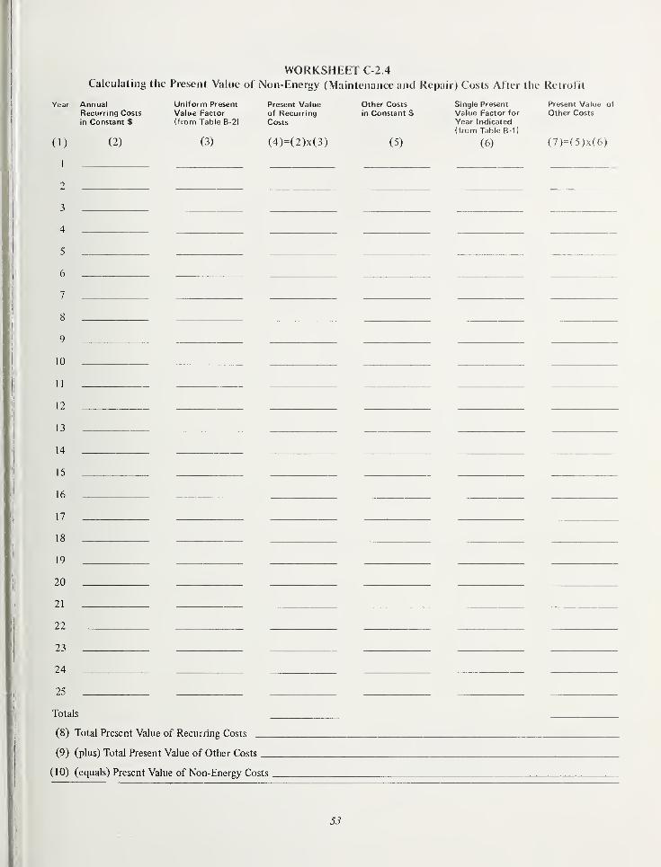
WORKSHEET C-2.4

Calculating the Present Value of Non-Energy (Maintenance and Repair) Costs After the Retrofit




(from Table B-1)

(1) (2) (3) (4)=(2)x(3) (5) (6) (7)=(5)x(6)

3

4

5

6

7

8

9

10

11

12

13

14

15

16

17

18

19

20

21

22

23

24

25

Totals




53

WORKSHEET C-2.5

Calculating the Present Value of Non-Energy (Maintenance and Repair) Cost Before the Retrofit



in Constant $ (from Table B-2) Costs Year Indicated(from Table B-1)

(1) (2) (3) (4)=(2)x(3) (5) (6) (7)=(5)x(6)

2

3

4

5

6

7

8

9

10

11

12

13

14

15

16

17

18

19

20

21

22

23

24

25

Totals




54

SUMMARY WORKSHEET C-3.1

Calculating the Total Life-Cycle Costs of the Energy Components of a New Building Project

( Design)

1 . Name of Agency


3. Location

4. Gross Floor Area AlTected

5. Expected iiconoiiiic Life of Building Design

6. Study Period

7. Present Value of Investment Cost


8. Present Value of Future Non-l:nerg> Costs


9. Total Present Value of Fnergy Costs

(Item 6 or 16, Worksheet C-3.2)

10. Total Life-Cycle Costs in Present Value S _(line (10) = lines (7) + (8) + (9))

55

o

O3

s.op

4>

S

3PQ

z

u uHUu

U

g i

!

2iA.0)

x:

00

op

c

su

5

o

z

OX)

"ooU

03

HoU

UJZu

u>«

w<CQ

u-OZo

<

X

ca o w— I/O

g tJ- O.2 o O

y >I

^ a.a> 3

0- £ ^

3 ci:

Tj- ^

>-

c U

c

HioC o

Cu oP -a

tr o

S o^ S

as o

(U Ct^ rnOa> cX 2

>

o

c cH oon

5£

>Ac^1)

II

 X

O '—

-

^ rr,

3 ^

O 00

.03 O> U

oH

^ +> c^

. .'

r-

'ah (uC o

a. oJ Cu wO

56

WORKSHEET C-3.3

Calculating the Present Value of Capital Investment Costs in a New Building Design

Year Investment Cost Salvage Single Present Present Value Present Valuein Constant $ Value at End of Value Factor for of Salvage of Investment for(Planning, Design, Study Period Year Indicated Year IndicatedConstruction, in Constant $ (from Table B-1

)

Replacement)

(1) (2) (3) (4) (5H3)x(4) (6M2)x(4)

0

1

3

4

5

10

25

Totals




57

WORKSHEET C-3.4

Calculating Non-Energy (Maintenance and Repair) Costs for a New Building Design




(from Table B-1)

(1) (2) (3) (4)=(2)x(3) (5) (6) (7M5)x(6)

9

10

11

12

13

14

15

16

17

18

19

20

21

22

23

24

25

Totals


(9) (plus) Total Present Value of Other Costs _(10) (equals) Present Value of Non-Energy Costs

38

APPENDIX DCOMPUTER PROGRAM

This Appendix contains a computer program written in BASIC*language for performing the Hfe-cycle cost calculations presented

in the guide. The program format is interactive, allowing the

analyst maximum flexibility in specifying the values of the para-

meters. This same program can be used to calculate the SIR for

retrofit projects on existing buildings (see Section 3) or to calcu-

late the total hfe-cycle costs of the energy-related componentsof a new buUding design (see Section 4).

The following is a listing of the program input statements:

Ll:CEU

5 LIN E (Sj 6J ? E^' (6) ? OS Cd) ? I (3? 8) ? R (4? 3 j ? N (3? 3)lU LIN U:^-i;6!

13 REN SINGLE PRESENT URL.UE DISCOMNT rORNULR15 HEP FNpi:::-::,zj=i.--i:i+;^jTZ

1? REN UNIFORN PRESENT URLUE DISCOUNT FCiRNULH INCLIJIUNG ENERGY• ESCRLHTION RRTE

30 DEF FtiiJ i ? 'i' ? Z )-

i 1 +Y j i;--:-'y"

J * (1 - f ( 1 -t- 'i' i .-'i: 1 +':< j i TZ J

PRINT "INPUT NRNE OF HGENC'i'"s© INPUT C}-$ \ 1 1

--.cr.":._! PRINT " INPUT PROJECT NfiNE"40 INPUT y^- (Pj

45 PRINT " INPUT LCCfiTION OF RGENCY"5U INPUT 0'$ ( >'

j

55 PRINT "TYPE 1 IF PROJECT IS FOR RN ENiSTIi-G EUILiaNG? 3 IFSO PRINT "IT IS FOR H NEN EUILLING"65 INPUT ij

78 PRINT "INPUT GROSS FLOOR RREH RFFEOTED ilN SQURRE FEET)"INPUT \ 4 I

'r-S PRINT " INPUT EXPECTED LIFE CP SYSTEM"3^1' INPUT Nl30 PRINT "INPUT EnPECTED LIFE OF BUILDING"95 INPUT R5i =1"!

ISO PRINT "INPUT STUDY PERIOD"105 INPUT N3110 IF OOl THEN 135115 LET D^^"SHUINGS"130 LET C^=" SPUED"125 LET_D5-;;FNISTING"130 GU iH l:-;0

135 LET E5=" COSTS"

*BASIC is an acronym for Begirmers AU-purpose SymboUcInstruction Code. For a description of the use of BASIC see

BASIC Language, Honeywell Information Systems Inc.,

August 1971.

59

143 LET C^^'COMSUriED"145 LET D5=^"MEW"158 PRINT "INPUT DISCOUNT KfiTE"155 INPUT D168 LET U==e165 LET Rlê170 LET Hi =8175 PRINT180 PRINT "ENERGY "B$185 PRINT198 PRINT "INPUT NUNIER OP ENERGY SOURCES USED"195 InPUT N4E88 MRT E=ZERi.&!.N4:i£05 FOR J=i TO N4£18 PRINT "INPUT ENERGY TYPE "J" RND UNIT (E.G. ELECTRICITY

(HERTING) rsKUHi "

£15 PRINT "NOTE: SEPRRRTE TYPE RND UNIT BY fi CONNR"P£8 INPNT E? L i 'i i i^- 1. i i

££5 PRINT "INPUT RNNURL RNOUriT OF "EsCJj " "C-^" EY THIS SYSTEM"£38 INPUT Ea^Jj£85 PRINT "INPUT LOCRL PRICE.-"U:? i J)

£48 INPUT Ei£?J:i£45 PRINT "INPUT LONG TERM ENERGY ESCRLRTION RRTE"£58 INPUT ECB.Jj£55 PRINT "TYPE 1 IF YOU HfiUE R SEPRRRTE SHORT TERM ENERGY"£68 PRINT "EsCRLRTION RRTE? 8 IF NOT"£65 INPUT S£78 IF 8=8 THEN £95£75 PRINT "INPUT SHORT TERM ENERGY ESCRLRTION RRTE"£88 INPUT EC4?Jj£85 PRINT "INPUT EXPECTED NUMBER OF YEARS THAT THIS RRTE CRN EE USED£98 INPUT Ei:5?Jj£95 PRINT388 NEXT J

KLM COnFUTE PRESEf-4T '.^RL.UE ENERGY SRv I NGS-'-'CDSTS318 FOR J=l TO N4315 LET EiS? Jj=Ê(l? Jj*Ei£? Jj3£8 IF S=e THEN 4153£5 IF D<>Ei:4nj£ THEN 348-:-:38 LE r L (•••? J j =-L (6? J)*L(5j J5335 on Tn :-;45

348 LET E(7? JJ=E>:6? Jj-FNUi:D?E(4? Jj ?Ei5? Jj )

345 LET 8(8? Jj^Ê i:£? Jj358 FOP K=i TO Ei:5?JJ355 lE'^ £i3,.n=::Fi'8^Ji+£!'8'.i'!*Fi4'. J"i

388 i-EXT k:

365 IF DOElSrJi THEri 388:278 LET 8 CJ J =L ( 1 ? J ) ^^Ê ( 8 ? J j ( tmR-E ( 5 ? j ) )

375 GO TO 3'^8

388 LET S i J ) =Ê (1 ? J J *E ( S • J J *FNU ( iJ ? E (8 ? J i ? N8-E ( 5 ? J )

)

385 LET 8 ( J j =--S ( J ) *FNP ( D ? E i 5 ? J j J

>:98 LET 5 i J j -8 ( J ) +L (.-

9 J j

:I-^5 i'Û Ti" 435488 IF D<>Ei3?J) THEN 415485 LET_8 ( Jj =E (6 ? J ) «N£41 H GO lU 4£8415 LET S i.j) =E (6!. J) *FrC! (D ? E CSj Jj 5 N£:i

60

4£y KLM S i: ^present '-..'RLLjE GF ENERG¥ :E:R'...' INGS4d5 LET U=! i+SiJj438 NEXT J435 PRINT448 PRINT "INUESTMENT COST"445 FPINT45i4 PRINT ''INPUT I NIT I PL INNESTNENt COST (ERSE VERRj "

455 INPUT I

468 PRINT ''INPUT riUNEER OF HliDITIOrifiL INNESTNENTS OR REPLhCENENTS"465 PRINT "OUER THE STUDY PERIOD"478 INPUT ri5

475 FOR K=l TO N54S8 PRINT "INPUT YERR THfiT COST OF RDDITIONRL INUESTNENT.-REPLROEMENT4S5 PRINT " # ^'K IS TO EE INCURRED"498 INPUT Id, K)495 PRINT "INPUT COST IN TODfiV'S DOLLRRS"508 INPUT Ii:S?Ki585 PRINT "INPUT SCRPP UfiLUE OF EOUIPNENT BEING REPLRCED (IF NONE OR"518 PRINT "NOT flPRLIOhBLE? TYPE 8 3

"

515 INPUT liSjKJ5E8 LET 1 = 1+1 K 3 *-FHP (Ds Id? K 3 3-1 ( 3 ? K 3 ^^FNP (D? Id? K 3 3

535 NEXT K=;:-;Pi PRINT "INPiiT RESIDURL UfiLUE OF INUESTNENT RT END OF S I UDY hLKlOi)"535 INPUT 19548 LET l9=I9*FNPiDjN£:3545 LET 1=1-19558 REM I IS PRESENT UfiLUE OF ir-iUECCCEDT COST555 PRINT508 PRINT "riON-ENERGY COSTS"505 PRINT578 LET R5=D5575 IF 0=1 _THEN 5S5

8 Kii ! i i "-i'-^U

585 PRir-iT "CRLCULRTIONS FOR "R5" SYSTEM",598 PRINT595 PRIiU "INPUT TOTRL YERRLY RMOUNT OF RNNURL RECURRIriO COSTS IN

TODRY-S688 INPUT R685 LET R=R*FNUi:D?85N£j618 PRINT "INPUT NUMBER. OF OTHER MfilNTENRNCE OR REPRIR COSiS THR i

"

615 PRINT "ROOUR ON H PERIODIC ERSIS"638 INPUT N6635 FOR J=i TO N6638 PRINT '^IriPUT RMOUNT OF RECURRIfiO COST "J635 ir^RUT Rd? J)648 PRiriT "INPUT FIRST YERR THRT THIS COST IS INCURRED RriD '^HE REkIUM'645 RRIiiT "OijER HHICH IT HILL RECUR (EYRMRLE: FOR R RECURRING COSi"658 PRINT "BEGINNING IN YERR 5 hflD OCCUR I NO EUERY 5 YERRS TYRE: -:.5 )'

655 INPUT RiP? Jj ?R(3! Ji

668 LET ( 4 r J J =R ( 1 ? J ) *Ff iP > lu R i 3 < (

3

665 FOR K=l TO INT ( iN£-h J3 1 .••-R CZu J 3 3

678 IF RiS? Ji-rK*RC?? j;i=N3 THEN 635€-[':ii RLM DGN-T rod recurring CGSTS THRT GEEUR L.RST VERR OF if-TUDV PER I DC6c:8 LL r R i' 4 , J j ! 4 . J "I 1 , . i s rr-^p \ p , ! 3 J ! +r * P i 'i !

635 mi K698 LET Ri=Rl+R (4^.33

695 NEYT J

61

7u5?iO715

— —

73Ur z.'-j'

74i^

74575Hi

7t87b5779I

1- _'

7SU

79u795860;-:m5

Sly81588S

8:39-.•-{=

840845h5m

; ._i

86G865878.-.—

~

£8;y

8888959089m59109159809859;30

9859409459509559609659709759;-:^

LET Rl=Rl-fRKLM NnN-RECURRING iZLi^TS

PRINTPRIr-iT "INPUT TUTRL NUMBER UR Nuri-RECURRING MRINTEriRNCE UR RERfilR"PRINT "Gusts THRT YuU HRUE TG ^^HKE"INPUT N7IP N7=0 THEN 778PGR J=l TO N7PRINT "INPUT GGST Ifi TGDHY^S TGLLRRS fifili YERR GP UGGURRENCE PGR"PRINT 'YiGN-REGURRING GGST YJ" iEYHMRLE= PGR R GGST GP ^580 IN "

PRINT "YERR 15? TYPE: 500^15 )

"

Ij-iPUT Nd, J) .MiP, J)LET M 1 =n 1 4-N i; 1 , J j

srNP x n , n ( 8 ? J j )

rc;:<T JIF R*="NEN" THEN 885LET R?="NEN"LET P-Rl+NlLET R1=0LET M1=0PRINTGfi in 585IP Q=R THEN 885LET li=Rl+NlLET_Y=^P-NGO i'G S40LET Y-Rl+NlPRINTPRINTPRINT "

PRINTPRINTPRINT "

PRINTPRINT "

PRINTPRINT "

PRINT'PRINT "

PRINTPRINTRRIfiTPRINT "

PRINTPRINT "

PRINTPRINT "

PRINTPRINT "

PRINTPRINT "

PRINTPRINT "

PRINTPGR K=l TG rH^

LET blKJ^SlK)PRINT "

NEXT K

RRGJEGT SUNnRRY REPORT

iMfiNE GP RGEr-iGY

RRGJEGT

LGGRTIGN OF RGENGY

GROSS FLOOR RRER RFFEGTEB

EYPEGTEL LIFE OF SY8TEN

EYFEGTEL LIFE GP EUILBING

STUBY PER I OB

BIS8GUNT RRTE

"Q$ iii

"G$ (8)

"GJ (3j

"G$i:4:i " SGURRE FEET"

"Ni" YERRS"

"0^(51" YERRS"

"N8" YERRS"

"B

(IN THGUSRNES i?)"

TOTRL PRESENT URLUE OP ENERGY ''B^

lOyy"E$ iKJ

"

I v: I

62

- i I J. I 1 I

Q-PiTi ]rrj

\

995 PRINT 1 ! ill—"1

1

PPT NT1 1 X

1818 PRINT1 i X t I 1

li TfiTHi Ppr'-PNT i iP! i'^r nr TNi iPPTMPNT rfiST I

PpTr-iT1 1 X 1 1 1

1 fiPCiX ^L.' 1

—

jr iTi-;- THEf i 1

1

1 I 1 X X 581— c_ 1 r —P'y \ MM Pi

-; Ci Z'LTi PPTr4Tr I J. ! I I

!l PT-PCPNJ ! IP]j :p fip Nnf •!—Pf-iFPNV PflPTs Pflp 11

PPT NT H rV T T T NT' TPMPi- 1 i _ 1 i 1;lj

1 _ 1 CI i

II pri C-' cl C-, pp T NT

i PT i.^—

1858 PK T r-iT3 1 . X t I 1

1 i Pizpc:rNT i iPI i iP pp r-'fiN-PHrprV PP'-TP PPiP II

185"-" PPTNT ppUprr-PT: PI TPPNPT7MP1860 PRINT1865 LET H= i !Jl88

1878 PRINT li pppepNT 1 iPI lip np fPIPNPP TN NnN-PNPpPy li

t ! -. X 1 1 1

li r-fi*-:TC; ii

j |T-;;r;L:i PPTNTt I -. X 1 1 1

J. '•

i PT T11 l_ 1 X

1898 PPTNT1 I -. X 1 [ 1

ii TflTfil PPP-;Pr-^T i 'Hi NP PH'iTNNS 'Tl1 X

1095 F'PTNT[ 1 . X : : i

1188 PRINT118"^". PPTNT

; t -. X t : t

ii LIRE-CYCLE COST NEfiSURES'^XX I

PPTNTt 1 X 1 1 I

i 1 1 i PT -Tl .•• Tu— X X

i J. i_PPT NT 1: SHUINGS TO INUESTMENT RRTIG il

—

1 1 - r r-. i i ^ 1

X X i PT ~'

-

-T 1 -T1 1 "15 PpTr^T

1 1 -. X 1 : i

11 NET SRUINGS IN PRESENT UfiLUE i!

1 1 diTiJ- X 1 1-'

PPTNT1 1 -. X 1 J I

1! DOLLRRS (IN THOUSRNDS1145 GO TO 1 iQi";X X

1158 LET :•• = ;••!• 1 88811 ""'"^^ PR.I NT i! PRESENT URLUE OR riOri-EriERGV COSTS 1 !

1 1 68 PPTNT{ 1 -. X 1 1 I

1!

p-pTNT1 1 -. X ! E i

X X 1 V-PpTNT

I -. X 1 1 1

1175 LET ZE1188 PRINT 1: TOTRL LIRE-CYCLE COSTS Iti PRESENTliS5 PRINT URLUE DOLLRRS (IN THOUSRNLS 5)1198 END

The above computer program is illustrated in the following

exam.ple of an energy conservation retrofit to an existing

building. This example is the same as that shown in the

worksheets in Section 3.

ir-iPUT NRNE OF RGEriCY? iiHTIONRL RriNINISTRRTIONINPUT PROJECT NRNE

ECi=;

INPUT LCCRTICii OF RGENCY. ;? URSHINGTON DC

63

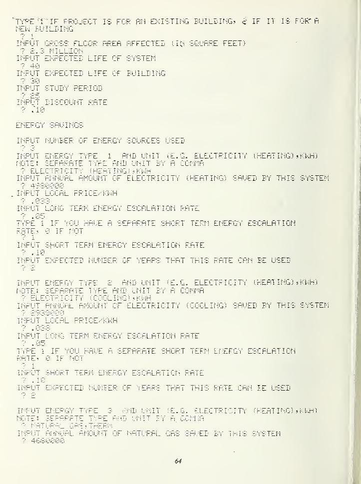
'type: '1 'IF PROJECT IS FOR AH EXISTING BUILDING? ^ IF IT IS t OR" Ht-EX'i BUILLING? 1

INPUT GROSS FLOOR RREfl RFFECTEIi lUi SQuRRE FEET)? S.S NlLLiONINPUT EKPECTED LIFE CP SYSTEM•? 40INPUT l:-;peoted life of building

INPUT STUDY PERIOD

INPUT DISCOUNT RRTE? /IS /

ENERG".' SRUir-iGS

INPUT NUMBER OF EriERGY SOURCES iJSED

INPUT ENERGY TYPE 1 RnD UNIT iE.G. ELECTRICITY (HERT ING)

?

KnH j

riOTE; EEPRRRTE TYPE RND UNIT BY R CCNMh? ELECTRI CI TY i HEhT ING J ? KMHINPUT fiiiNURL RMOUNT OF ELECTRICITY ihERTING) SRUED BY THIS SYSTEM

. INPUT LOCRL PRICE.--k;NH

? ,0S>:INPUT LONG TERM ENERGY ESCRLRTION RRTE? .05

TYPE i IF YOU HRUE R SlPmRhTE SHORT TERM ENERGY ESCRLRTIOriRRTE? 0 IF NOT? 1

. INPUT SHORT TERM ENERGY ESCRLRTION RRTE. 10

INPUT EYPECTED iiUMBER OF YERRS THRT THIS RRTE CRN EE USED

IhPUT ENERGY TYPE £ RND UNIT ^:E.G. ELECTRICITY (HlR i ING) ? KNH j

NOTE^ SEPRRRTE T^iP'E RtiD UNIT BY R COnrlR? ELECTR I C I TY ( COOL Im ) KMHINPUT HririUHL RMOUriT CP ELECTRICITY iCCOLINGj SfiMFD BY THIS SYSTEM? £S:sijGuO

INPUT LOCRL PRICE.--KMH:'

. 0>^S

INPUT Lur^G TERM ENERGY ESCRLRTICii RRTE? .05

T^PE 1 IF YOU HRUE R SEPRRRTE SHORT TERN ErCPGY ESCRLRTIONRRTEi. 0 IF NOT

- 1

INPUT SHORT TERM EiiERGY ESCRLRTION RRTE. 10

INPUT EXPECTED NUMBER OF ^yERRS THRT THIS RRTE CRri BE USED

INPUT ENERGY T'iPE S RND UNIT lE.G. ELECTRICITY i HERT ING) ? K LHiNOTE: ::;rppppTr jvpe hND UNIT EY R CCMtih

r-RTuRHL GR'E? THERMINPUT RriNURL PMCUriT OF NRTURRL GRS SR^/ED BY THIS SYSTEn? 4680000

64

INPUT LOCRL PRICr..-THERM

INPUT^LOMG TERM ErCRGY E&CF.LRTIOM RRTE.81-

TYPE 1 IF YOU HhUE fl SEPRRRTE SHORT TERM EhERGY ESCRLRTIONRRTEr 0 IF j'lOT

^ 1

INPUT SHORT TERM Er-;ERGY ESCRLRTIOri RRTE? .06INPUT EFFECTED NUMBER OF YERRS THRT THIS RRTE CRN BE USED

INUESTNENT LOST

INPUT_INITIfiL INUESTNENT COST (BASE YERRi

INPUT NUMBER OF RDDITIONRL INUESTNEriTS OR REPLROEMENTSOUER THE STUDY PERIOD

INPUT YERR THRT COST OF RDDITIONRL I NUESTMENT.--REPLRCEMENT #IS TO EE INCURRED•? 1

INPUT COST IN TODRY'S DOLLRRS

INPUT SCPRP URLUE OF EQUIPMENT BEING REPLRCED (IF NONE ORNOT RPPLICRELEj TYPE OJ

INPUT YERR THRT COST OF RDDITIONRL I NUESTMENT.-REPLRCEMENT #IS TO BE INCURRED? 10INPUT COST IN TODRY' S DOLLRRS

INPUT SCRRP URLUE OF EQUIPMENT BEING REPLRCED (IF NONE ORNOT RPPLICRBLE? TYPE 0'

0INPUT RESIDURL URLUE OF ItiUESTMENT RT END OF STUDY PERIOD? EOOyOu

NON-ENERGY COSTS

CRLCULRTIONS FOR EXISTING SYSTEM

INPUT TOTRL^YERRLY RMOUNT OF RNriURL RECURRING COSTS IN TODRY? ISOOuOINPUT riUMBER OF OTHER MRINTENRNCE OR REPRIR COSTS THRT OCCURON R PERIODIC BPS IS? i

INPUT RMOUNT OF RECURRING COST 1

INPUT FIRST YERR THRT THIS COST IS INCURRED RND THl PERIODniJER MHTCH IT MILL RECUR (LiKRMPLE' FOR H KLCURRIriC CCS!_BEGINNir-iG Ii i YERR 5 RND OCCUR I NG EUEPY 5 YlhkS lYrE? b?:i. )

rr ~:" - ?

TNPMT TmThL ilUMBER OF NuN-RECUFR:ING MRIhTENHNCE OR REPRIRCOSTS THRT YOU HRUE TO MhkE? y

65

CfiLCULFiTIOHS FOR TiEN SYSTEM

IHPUT TOTF.L YERRLY hMDUMT OF RNriURL RECURRING COSTS IH TOLRY'

IHPUT NUMEER OF OTHER riRIHTEHRriCE OR-REPfilR COSTS THfiT OCCUROH H PER I era C EfiSIS

7' 1

IHPUT flHOUriT OF RECURRIHG COST 1

IHPUT FIRST YERR THRT THIS COST IS IH(OUER NHICH IT NILL RECUR (EHRHPLE: FORBEG I Hh I NG IH YERR 5 RHD OCCUR I HG EUER'y

jpRED PHE THE PERIODR RECURRING COST5 YERRS TYPE: i

IHPUT TOTRL HUMEER OF HOH-RECURRIiiG HRIHTEHRNCE OR REPRIRCOiETS THRT VO'U HRUE TO MRKE

RF:OJECT SiJMnRRY REPORT

HRME OF RGEHOY

PROJECT

LOCRTIOH OF RGEHCY

GROSS FLOOR RRER RFFECTEE

EXPECTED LIFE OF SYSTEM

EXPECTED LIFE OF BUILDING

STUDY PERIOD

DISCOUi-iT RRTE

HRT I OHRL RDM I N I STRRT I ON

ECS

NRSHIHCTON DC

£.3 MILLION SOURRE FEET

40 YERRS

30 YERRS

£5 YERRS

. 1

s S ft

(IH THOUSRHDS 5!

TOTRL PRESEtiT URLUE OF EriERGY SfiUINGS

ELECTRICITY J.HEfiTING) £596.ELECTR 1 0 1 TY iCOOL I HG ) 1 (-58 . 79riRTURRL GRS 1S4G4.3

TOTRL ££759.

1

TOTRL PRESENT URLUE OF INUESIMENT COST 1384.91

PRESEriT URLUE OF NON-ENERGY COSTS FOREXIST IiiG SYSTEM 1284.47

PRESEriT URLUE OF huH-EHERGY COSTS FORPROPOSED RLTERHRT I UE £G£4 . 33

66

rRLSEhT URLiJE OF CHhhGE IN riUh-EHERG'i'LLibT;i. -739. y5E:

TOTRL RREbEHT URLUE SRUIMGS £2919.3

LIFE-CVCLE COST NEROilJRES;

SfiUINGS TO IriUESTrCHT RRTIO 15.8994

r-iET SRUINGS IN PRESENT URLUEnOLLRRS (IN THOUSfiHDS ?) £6634.4

RUNNING TIME: 6.6 SECS I.--0 TIME : 37.3 SECS

(57

APPENDIX E

SELECTED ANNOTATEDREFERENCES

1. Grant, Eugene L. and Ireson, W. Grant. Principles of

Engineering Economy. New York: Ronald Press,

5th Edition, 1970.

A widely used textbook on engineering economics.

Contains a comprehensive description of discounting

with emphasis on investment analysis. Provides tables of

discounting formulas and factors.

2. The American Institute of Architects. Life Cycle

Cost Analysis: A Guide for Architects. Washington,

D.C., 1977.

An easy-to-understand guide to fundamental LCC

principles, directed primarily at architects who are not

experienced in LCC analysis.

3. Reynolds, Smith & Hills, Architects -Engineers,

Planners. Life-Cycle Costing Emphasizing Energy

Conservation; Guidelines for Investment Analysis.

Energy Research Development Administration

Manual 76/130, Revised May, 1977.

A detailed LCC analysis handbook for ERDA, focusing

on the retrofitting of existing facilities for energy con-

servation. Describes procedures to use and provides

forms to complete for conducting investment analysis

of energy conservation projects.

4. Booz-Allen and Hamilton, Inc. Life-Cycle Costing in

the Public Building Service. Prepared for the

General Services Administration, Vol. I, 1976,

andVoL II, 1977.

A comprehensive manual aimed primarily at evaluating

alternative new building designs, that outUnes LCCprocedures for the PubUc Building Service of GSA.

Vol II lists selected computer programs for simulating

the energy loads of buildings.

5. Office of the Chief of Engineers, Department of the

Army. Engineering Instructions for Preparation ofFeasibility Studies for Total Energy, Selective

Energy, and Heat Pumps. July 1 , 1977.

Contains life-cycle costing instructions in a 10-page

appendix that provides a step-by-step illustration of

the computation of the present values of alternative

energy systems for a building v/ith the base period de-

fined as the midpoint of the construction period.

Provides a glossary of terms and instructions for deter-

mining heating and cooUng loads, initial costs, and

maintenance costs.

6. Richard S. Brown, et. al. Economic Analysis

Handbook. Prepared for the Department of the

Navy, June, 1975.

Explains the concepts and techniques of economic

analysis for the purpose of providing official guidance

for the preparation of economic evaluation of invest-

ment decisions. Includes a discussion of the selection of

a 10% discount rate for evaluating government invest-

ments; a section on cost analysis that describes the

treatment of such items as residual values and personnel

costs, using three techniques for estimating costs; a

chapter on the treatment of inflation and conversion

of cost estimates to budgetary amounts; and provides

illustrations of techniques throughout.

7. Harold E. MarshaU and RosaUe T. Ruegg. "Life-

Cycle Costing Guide for Energy Conservation

in Buildings." Energy Conservation Through

Building Design. McGraw-Hill Architectural

Record Books, In press.

Provides an overview of the state-of-the-art of Ufe-cycle

costing appUed to energy conservation in buildings.

Describes selected appUcations of LCC analysis, includ-

ing (1) determining the optimal amount of insulation

in existing houses; (2) the selection and use of windows

in houses; (3) the choice between solar and alternative

heating systems; and (4) the development of standards

for efficient energy conservation in buildings.

8. PubUc Technology, Incorporated. Energy Conser-

vation Retrofit for Existing Public and Institutional

Facilities. Prepared for National Science Founda-

tion (RANN), Washington, D.C., 1977.

Devoted primarily to providing assistance to public offi-

cials considering energy conservation in existing public

buildings. Provides assistance in making management

decisions for implementation of energy conservation

programs, including development of a plan, establish-

ment of schedules, selection of buildings, preliminary

estimation of energy savings, development of work

statements, and estimation of fees and construction

costs. Describes four phases in the management of

energy conservation: (1) the study of current energy

consumption, (2) building survey and engineering

analysis, (3) implementation, and (4) monitoring. Does

not provide the details necessary for conducting engi-

neering analysis nor life-cycle cost analysis. Emphasizes

fast-payback retrofit projects. Appendices include

Usts of retrofit options by climate zones, sample forms

for studies of energy consumption, and a list of

computer programs for energy conservation analysis.

The bibUography gives a number of references to guides

for reducing energy consumption of buildings through

retrofit and initial design.

68

9. National Bureau of Standards. Technical Guidelines

for Energy Conservation. Prepared for the Air Force

Civil Engineering Center, NBSIR 77-1238,

AFCEC-TR-77-12, June, 1977.

Provides detailed technical material on various energy

conservation actions for existing Air Force facilities and

utility systems. Intended to serve as a working document

for engineers and technical personnel. Includes coverage

of equipment for providing hot water, space heating and

cooling, Ughting and humidification; central plant sys-

tems for hot water, steam, and chilled water. Discusses

energy conservation measures for exterior building enve-

lopes and for mechanical systems; describes the building

energy survey and measurements for identifying energy

conservation potential; and explains in brief the econo-

mic analysis. Appendices provide information on heat

transfer, solar energy systems, distribution systems, and

computer programs.

10. Hittle, D.C. The Building Loads Analysis and

System Thermodynamics (BLAST) Program,

Volume L Users Manual. U.S. Army Construction

Engineering Research Laboratory (CERL), Tech-

nical Report E-119, September, 1977.

Provides detailed user instructions for the BLASTprogram for the analysis of building energy loads.

1 1 . Kusuda, Tamami. NBSLD, the Computer Program

for Heating and Cooling Loads in Buildings. Nation-

al Bureau of Standards, BSS 69, July, 1976.

Describes the methodological basis of the NBSLDprogram for the analysis of building energy loads.

12. Federal Energy Administration. Identifying

Retrofit Projects for Buildings. FEA/D-76-467,

GPO 041-018-00129-8, September, 1976.

Handbook designed to be used by building owners,

managers, operators, and occupants to identify quick

payback retrofit projects in existing buildings. Provides

tools for coordinating the energy savings, cost savings,

capital costs, and simple payback periods for the

options identified. Suggests a format for writing up the

options, energy quahfications, and reporting the overall

surveys for one or several buildings.

13. Federal Energy Administration. Guidelines for

Saving Energy in Existing Buildings, ECMLFEA/D-75-359, GPO 041-018-000-79-8, June 16,

1975.

A manual for building ovmers and operators for con-

serving and managing energy use in buildings (including

office buildings, retail stores, hospitals, schools, libraries,

houses, and apartments) with relatively small investments.

14. Federal Energy Administration. Manual forEngineers, Architects, and Operators, ECM2.FEA/D-75-358, GPO 041-018-000-80-1.

A Guide intended for engineers, architects, and skilled

building operators who are responsible for administering,

advising, and implementing energy conservation pro-

grams which involve additional and more complex

measures than those included in ECMl. Includes manyconservation measures which can result in energy

savings of 15-25% with an investment cost that can be

recovered within 10 years through reduced operational

cost.

1 5. Department of Energy. Energy Conservation

Compendium. DOE Manual in Preparation to

support implementation of Executive Order 12003.

A compendium which includes those pubHcations de-

signed specifically for use in plaiming and carrying out

energy conservation programs. Purpose is to provide

energy coordinators, plarmers, and related managing

professionals with tools they may require to success-

fully plan, implement, and manage energy conservation

programs. Contains abstracts of publications by manyFederal and state agencies and information on where

particular tools may be obtained.

16. State of California, Energy Resources Conservation

and Development Commission Conservation Divi-

sion. Energy Conservation Design Manual forNewNonresidential Buildings. October, 1977.

Describes the procedures, calculations, and documenta-

tion regarding energy conservation that are required

prior to the application for a building permit in Cahfor-

nia. Describes calculation procedures for various energy

analyses and provides documentation forms. Provides

a brief description of life-cycle costing calculations as

related to meeting the requirements of the California

Energy Conservation Standards for New Nonresidential

Buildings.

17. Executive Office of the President. "Relating to

Energy Policy and Conservation." Executive Order

12003. July 20, 1977.

Amended Executive Order No. 11912, dated April 13,

1976, to require each executive agency that now main-

tains buildings to submit to the Administrator of the

FEA a ten-year plan designed "to the maximum extent

practicable" to meet specified goals for energy conser-

vation in Federal buildings. Calls for the establishment

of a "practical and effective "method for estimating

and comparing life-cycle capital and operating costs for

Federal residential, commercial, and industrial buildings.

Requires the use of this method by Federal agencies in

developing their ten-year plans, annual reports, and

budget estimates for meeting the goals of reduced energy

usage.

18. Laughlin, Qonnie B.Q. Energy Conservation, TheState of the States. National Governors' Associa-

tion, Center for Policy Research. Washington, D.C.

69

Provides an overview of the proposed plans for energy

conservation programs prepared by States in response to

the 1975 Energy PoUcy and Conservation Act (EPCA).

Includes detailed descriptions of the initiatives of

selected States.

19. Cooke, Patrick W. and Eisenhard, Robert M. Build-

ing Energy Conservation Programs — A Preliminary

Examination ofRegulatory Activities at the State

Level. National Bureau of Standards, NBSIR 77-

1259, June, 1977.

Describes the current regulatory status and degree of im-

plementation of building energy conservation programs

at the State level, including those programs that deal

with solar energy. Based on a survey of 21 selected

States, reports common problems experienced at the

State level in the promulgation and implementation of

buUding energy conservation regulations.

20. "Project Independence Evaluation Series," Federal

Register. Vol. 42, No. 73, April 15, 1977.

Gives FEA's projected energy prices developed from

March 30, 1977 Reference Case results of the Project

Independence Evaluation System (PIES), an integrated

model of the domestic energy system. Prices of oU, gas,

coal, and electricity are projected by region, by year,

to 1991.

24. Ruegg, Rosalie T. and Sav, G. Thomas. Microecono-

mics of Solar Energy. National Bureau of Standards,

BSS, In Press.

A comprehensive reference report that explains howalternative economic evaluation methods may be used

to evaluate the economic efficiency of solar energy sys-

tems for residential, commercial, and institutional

buildings. Describes the major components of costs and

savings associated with solar energy systems, including

the various types of system costs, energy costs and

savings, taxes, and government incentives. Explains and

illustrates the optimization of a solar energy system for

maximum net savings.

25. Energy Resource Center, University of Illinois.

Selection and Assessment Methodology of Weatheri-

zation Retrofit Options for Multi-Family Buildings.

Prepared for the National Bureau of Standards,

December 1977.

Describes a detailed approach to the problem of ranking

interdependent projects.

21. Executive Office of the President, Office of

Management and Budget. "Comparative Cost

Analysis for Decisions to Lease or Purchase Gen-

eral Purpose Real Property." Circular No. A-104,

June 14, 1972, Attachment.

22. U.S. Department of Labor, Bureau of Labor Statis-

tics. Monthly Labor Review.

Provides price indices that can be used to convert cur-

rent dollars to constant doUars.

23. Petersen, Stephen R. Retrofitting Existing Housing

for Energy Conservation An Economic Analysis.

National Bureau of Standards, BSS 64, 1974.

A technical study which develops an economic model

for determining the optimal combination and level of

energy conservation retrofit techniques in existing

houses.

70

NBS-114A (REV. 7-73)

U.S. DEPT. OF COMM.BIBLIOGRA,PHIC DATA

SHEET

1. PURl ICATION OR RFPORT NO

NBS BSS-113

2> Ciov t Ac c c s -S 1 oil

N,,.

3. ipicDi A( ( cs.sion No.

4. TITLE AND SUBTITLE

Life-Cycle Costing

A Guide for Selecting Energy Conservation Projects forPublic Buildings

,

5. Publication Date

September 19786. Performing Organization C-txic

7. AUTHOR(S)R.T. Ruegg, J.S. McConnaughey, G.T. Sav, K.A. Hockenbery

8. Performing Organ. Report No.

9 PFRFORMING ORG ANI7 ATION NAMF AND AHHR

NATIONAL BUREAU OF STANDARDSDEPARTMENT OF COMMERCEWASHINGTON, D.C. 20234

10. Project/Task/Work Unit No.

11. Contract/Grant No.

^ 2» Spon ^ or 1 3niZ3tton Nsmc snd Comp Ictc Address trGGt, C i ty , S tQ tG , ^IP

y

Department of Energy1111 20th St. N.W.Washington, D.C. 20545

13. Type of Report & PeriodCovered

Final

14. Sponsoring Agency Code

15. SUPPLEMENTARY NOTES

Library of Congress Catalog Card Number: 78-60009416. ABSTRACT (A 200-word or less [actual summary of most significant information. If document includes a significant

bibliography or literature survey, mention it here.)

This report provides a step-by-step guide for conducting life-cycle costevaluations of energy conservation projects for public buildings. It explainsthe use of life-cycle costing analysis to evaluate and rank the cost effectivenessof alternative energy conservation retrofit projects to existing public buildings,and to select the most cost-effective design for new buildings. Worksheets,illustrated with a realistic example, and a computer program are provided.

This guide is compatible with a life-cycle costing guide prepared for theDepartment of Energy for use in the Federal Energy Management Program by FederalAgencies. The purpose of this report is to provide a guide to state and localgovernments for use in their energy conservation programs.

17. KEY WORDS (six to twelve entries; alphabetical order; capitalize only the first letter of the first key word unless a proper

name; separated by semicolons)

Building economics; economic analysis; energy conservation; engineering economics;investment analysis; life-cycle cost analysis

18. AVAILABILITY E Unlimited

1 For Official Distribution. Do Not Release to NTIS

5ri Order From Sup. of Doc., U.S. Government Printing Office

Washington, D.C. 20402, SD Steele No. SN003-003-01980-1

1 1Order From National Technical Information Service (NTIS)Springfield, Virginia 22151

19. SECURITY CLASS(THIS REPORT)

UNCL ASSIFIED

21. NO. OF PAGES

76

20. SECURITY CLASS(THIS PAGE)

UNCLASSIFIED

22. Price

$2.75

j

USCOMM-DC 29042-P74

I

llUilleat

Manayeinent

EwBiookA typical plant can save about 20 percent of its

fuel—just by installing waste heat recovery equip-

ment. But with so much equipment on the market,

how do you decide what's right for you?

Find the answers to your problems in the WasteHeat Management Guidebook, a new handbookfrom the Commerce Department's National Bureauof Standards and the Federal Energy Administra-

tion.

The Waste Heat Management Guidebook is de-

signed to help you, the cost-conscious engineer or

manager, learn how to capture and recycle heat

that is normally lost to the environment during in-

dustrial and commercial processes.

The heart of the guidebook is 14 case studies of

companies that have recently installed waste heat

recovery systems and profited. One of these appli-

cations may be right for you, but even if it doesn't

fit exactly, you'll find helpful approaches to solving

many waste heat recovery problems.

In addition to case studies, the guidebook contains

information on:

• sources and uses of waste heat

• determining waste heat requirements• economics of waste heat recovery• commercial options in waste heat recoveryequipment

• instrumentation

• engineering data for waste heat recovery• assistance for designing and installing waste

heat systems

To order your copy of the Waste Heat ManagementGuidebook, send $2.75 per copy (check or moneyorder) to Superintendent of Documents, U.S. Gov-ernment Printing Office, Washington, D.C. 20402.

A discount of 25 percent is given on orders of 100

copies or more mailed to one address.

The Waste Heat Management Guidebook is part of

the EPIC industrial energy management program

aimed at helping industry and commerce adjust to

the increased cost and shortage of energy.

U.S. DEPARTMENT OF COMMERCE/National Bureau of Standards

FEDERAL ENERGY ADMINISTRATION/ Energy Conservation and Environment

There'sanewlookto...

. . . the monthlymagazine of the Nation-

al Bureau of Standards.

Still featured are special ar-

ticles of general interest oncurrent topics such as consum-er product safety and building

technology. In addition, new sec-

tions are designed to . . . PROVIDESCIENTISTS with illustrated discussions

of recent technical developments and

work in progress . . . INFORM INDUSTRIALMANAGERS of technology transfer activities in

Federal and private labs. . . DESCRIBE TO MAN-UFACTURERS advances in the field of voluntary and

mandatory standards. The new DIMENSIONS/NBS also

carries complete listings of upcoming conferences to be

held at NBS and reports on all the latest NBS publications,

with information on how to order. Finally, each issue carries

a page of News Briefs, aimed at keeping scientist and consum-alike up to date on major developments at the Nation's physi-

cal sciences and measurement laboratory.

(please detach here)

SUBSCRIPTION ORDER FORM

Enter my Subscription To DIMENSIONS/NBS at $12.50. Add $3.15 for foreign mailing. No additional

postage is required for mailing within the United States or its possessions. Domestic remittances

should be made either by postal money order, express money order, or check. Foreign remittances

should be made either by international money order, draft on an American bank, or by UNESCOcoupons.

Send Subscription to:

Remittance Enclosed

(Make checks payable

to Superintendent of

Documents)

Charge to my Deposit

Account No.

NAME-FIRST, LAST

COMPANY NAME OR ADDITIONAL ADDRESS LINE

STREET ADDRESS

I I I I I I I I I I I I I I I

I I I I I I I I I I I I I I I I 3

MAIL ORDER FORM TO:

Superintendent of Documents

Government Printing Office


PLEASE PRINT

Announcement of New Publications

of the

National Bureau of Standards

Superintendent of Documents,Government Printing Office,

Washington, D. C. 20402

Dear Sir:

Please add my name to the announcement list of newpublications as Issued by the National Bureau of Standards.

Name

Company

Address

City State Zip Code

(Notification Key N519)

0-77-47{^ U.S. GOVERNMENT PRINTING OFFICE : 1978 O—273-736

NBS TECHNICAL PUBLICATIONS

PERIODICALSJOURNAL OF RESEARCH—The Journal of Researchof the National Bureau of Standards reports NBS research

and development in those disciplines of the physical andengineering sciences in which the Bureau is active. Theseinclude physics, chemistry, engineering, mathematics, andcomputer sciences. Papers cover a broad range of subjects,

with major emphasis on measurement methodology, andthe basic technology underlying standardization. Also in-

cluded from time to time are survey articles on topics closely

related to the Bureau's technical and scientific programs. Asa special service to subscribers each issue contains completecitations to all recent NBS publications in NBS and non-

NBS media. Issued six times a year. Annual subscription:

domestic $17.00; foreign $21.25. Single copy, $3.00 domestic;

$3.75 foreign.

Note: The Journal was formerly published in two sections:

Section A "Physics and Chemistry" and Section B "Mathe-matical Sciences."

DIMENSIONS/NBSThis monthly magazine is published to inform scientists,

engineers, businessmen, industry, teachers, students, andconsumers of the latest advances in science and technology,

with primary emphasis on the work at NBS. The magazinehighlights and reviews such issues as energy research, fire

protection, building technology, metric conversion, pollution

abatement, health and safety, and consumer product per-

formance. In addition, it reports the results of Bureau pro-

grams in measurement standards and techniques, properties

of matter and materials, engineering standards and services,

instrumentation, and automatic data processing.

Annual subscription: Domestic, $1 1.00; Foreign $13.75

NONPERIODICALSMonographs—Major contributions to the technical liter-

ature on various subjects related to the Bureau's scientific

and technical activities.

Handbooks—Recommended codes of engineering and indus-

trial practice (including safety codes) developed in coopera-

tion with interested industries, professional organizations,

and regulatory bodies.

Special Publications—Include proceedings of conferences

sponsored by NBS, NBS annual reports, and other special

publications appropriate to this grouping such as wall charts,

pocket cards, and bibliographies.

Applied Mathematics Series—Mathematical tables, man-uals, and studies of special interest to physicists, engineers,

chemists, biologists, mathematicians, computer programmers,and others engaged in scientific and technical work.

National Standard Reference Data Series—Provides quanti-

tative data on the physical and chemical properties of

materials, compiled from the world's literature and critically

evaluated. Developed under a world-wide program co-

ordinated by NBS. Program under authority of National

Standard Data Act (Public Law 90-396).

NOTE: At present the principal publication outlet for these

data is the Journal of Physical and Chemical Reference

Data (JPC'RD) published quarterly for NBS by the Ameri-can Chemical Society (ACS) and the American Institute of

Physics (AIP). Subscriptions, reprints, and supplementsavailable from ACS, 1155 Sixteenth St. N.W., Wash., D.C.20056.

Building Science Series—Disseminates technical information

developed at the Bureau on building materials, components,systems, and whole structures. The series presents research

results, test methods, and performance criteria related to the

structural and environmental functions and the durability

and safety characteristics of building elements and systems.

Technical Notes—Studies or reports which are complete in

themselves but restrictive in their treatment of a subject.

Analogous to monographs but not so comprehensive in

scope or definitive in treatment of the subject area. Oftenserve as a vehicle for final reports of work performed at

NBS under the sponsorship of other government agencies.

Voluntary Product Standards—Developed under procedures

published by the Department of Commerce in Part 10,

Title 15, of the Code of Federal Regulations. The purpose

of the standards is to establish nationally recognized require-

ments for products, and to provide all concerned interests

with a basis for common understanding of the characteristics

of the products. NBS administers this program as a supple-

ment to the activities of the private sector standardizing

organizations.

Consumer Information Series—Practical information, based

on NBS research and experience, covering areas of interest

to the consumer. Easily understandable language andillustrations provide useful background knowledge for shop-

ping in today's technological marketplace.

Order above NBS publications from: Superintendent ofDocuments, Government Printing Office, Washington, D.C.20402.

Order following NBS publications—NBSIR's and FIPS fromthe National Technical Information Services, Springfield,

Va. 22161.

Federal Information Processing Standards Publications

(FIPS PUB)—Publications in this series collectively consti-

tute the Federal Information Processing Standards Register.

Register serves as the official source of information in the

Federal Government regarding standards issued by NBSpursuant to the Federal Property and Administrative Serv-

ices Act of 1949 as amended. Public Law 89-306 (79 Stat.

1127), and as implemented by Executive Order 11717

(38 FR 12315, dated May 11, 1973) and Part 6 of Tide 15

CFR (Code of Federal Regulations).

NBS Interagency Reports (NBSIR)-—A special series of

interim or final reports on work performed by NBS for

outside sponsors (both government and non-government).

In general, initial distribution is handled by the sponsor;

public distribution is by the National Technical Information

Services (Springfield, Va. 22161) in paper copy or microfiche

form.

BIBLIOGRAPHIC SUBSCRIPTION SERVICES

The following current-awareness and literature-survey bibli-

ographies are issued periodically by the Bureau:

Cryogenic Data Center Current Awareness Service. A litera-

ture survey issued biweekly. Annual subscription: Domes-tic, $25.00; Foreign, $30.00.

Liquified Natural Gas. A literature survey issued quarterly.

Annual subscription: $20.00.

Superconducting Devices and Materials. A literature survey

issued quarterly. Annual subscription: $30.00. Send subscrip-

tion orders and remittances for the preceding bibliographic

services to National Bureau of Standards, Cryogenic Data

Center (275.02) Boulder, Colorado 80302.

U.S. DEPARTMENT OF COMMERCENational Bureau of StandardsWashington, D.C. 20234

OFFICIAL BUSINESS

Penalty for Private Use, $300

POSTAGE AND FEES PAIDU.S. DEPARTMENT OF COMMERCE

COM-215

SPECIAL FOURTH-CL^SS RATEBOOK