lifetime assessment of electrical insulation

Chapter 11

Lifetime Assessment of Electrical Insulation

Eyad A. Feilat

Additional information is available at the end of the chapter

http://dx.doi.org/10.5772/intechopen.72423

Provisional chapter

Lifetime Assessment of Electrical Insulation

Eyad A. Feilat

Additional information is available at the end of the chapter

Abstract

In this chapter, a review of the Weibull probability distribution, probability ranking,and the Weibull graphical estimation technique is presented. A review of single-stressand multiple-stress life models of electrical insulation is also introduced. The chapteralso describes the graphical, linear and multiple linear regression techniques used inestimating the parameters of the aging models. The application of maximum likeli-hood estimation technique for estimating the parameters of combined life models ofelectrical insulation is illustrated.

Keywords: life models, aging, insulation, Weibull probability, maximum likelihoodestimation, least square estimation

1. Introduction

A lifetime analysis of electrical insulation failure is an approach that relies on statisticalanalysis of data that are attributed to the breakdown of the electrical insulation due to thepresence of degrading stresses, such as electrical, thermal and other environmental factors. Thelifetime analysis can provide statistical information about the electrical insulation such aslifetime characteristics, probability of failures, lifetime percentiles or any time percentile undernormal operating conditions. In this approach, the insulation life is determined by measuringthe time-to-breakdown of identical specimens of the solid insulation subjected to life tests [1–5]. Obtaining life data under normal operating conditions is a very time consuming and costlyprocess, rendering it impractical. Besides, it is important to observe modes of failure of theelectrical insulation to better understand the prevailing mechanisms of breakdown. Conse-quently, electrical insulation design engineers and material scientists devised methods to forcethe insulation to fail in shorter periods of time. These methods seek to accelerate the failures ofinsulation samples by applying stresses at levels that exceed the levels that the insulation willencounter under normal operating service conditions. Acceleration is accomplished by testing

© The Author(s). Licensee InTech. This chapter is distributed under the terms of the Creative Commons

Attribution License (http://creativecommons.org/licenses/by/3.0), which permits unrestricted use,

distribution, and eproduction in any medium, provided the original work is properly cited.

DOI: 10.5772/intechopen.72423

© 2018 The Author(s). Licensee IntechOpen. This chapter is distributed under the terms of the CreativeCommons Attribution License (http://creativecommons.org/licenses/by/3.0), which permits unrestricted use,distribution, and reproduction in any medium, provided the original work is properly cited.

the insulation (specimen or device) using single or combined high stress levels which couldinvolve electrical, thermal or environmental stresses for either short periods (few seconds orminutes) or long periods (few hours or days) [6]. The accelerated test data are then consideredas a base for extrapolation to obtain an estimate of the lifetime of the insulation when thedevice or material is operated at normal operating conditions for relatively long time periods(decades) of years [7–27].

Times-to-breakdown obtained by accelerated life (aging) tests are analyzed using an underly-ing lifetime probability distribution. The probability distribution can, correspondingly, be usedto make predictions and estimates of lifetime measures of interest at the particular stress level.This is accomplished by projecting or mapping lifetime measures from high stress level to aservice level. It can be assumed that there is some model (or function), which can be describedmathematically, that maps the lifetime estimate from the high stress level to the service level,and can be as simple as possible (i.e. linear, exponential, etc.) [28–37]. The parameters of thelifetime models can be estimated by combining the proposed life models with the Weibullprobability distribution function. Maximum likelihood estimation can be used to estimate theparameters of the combined Weibull-electrical-thermal models using experimental dataobtained by measuring time-to-breakdown of the insulation.

2. Weibull probability distribution

The Weibull distribution has been widely recognized as the most common distribution inbreakdown testing of solid dielectric insulation and in reliability studies [28–31, 37–40]. Itspopularity is attributed to the many shapes it attains for various values of the shape parameter(β). It can model a large variety of data and life characteristics. The distribution also has theimportant properties of flexibility and a closed form solution for the integral of the Weibullprobability density function (pdf). This latter property is important for easy determination ofthe Weibull cumulative probability function (cdf) and its corresponding parameters. There arethree forms of the Weibull cumulative probability distribution functions, namely, the three-parameter Weibull distribution, the two-parameter Weibull distribution and the mixedWeibull distribution. In life data analysis, the two-dimensional Weibull distribution is oftenused to describe the time-to-breakdown of solid dielectric insulation with voltage, as it is aconvenient way for deriving the V-t characteristic or life models. The two-parameter Weibullpdf and cdf distributions are defined as:

f t;α;β� � ¼ β

αtα

� �β�1

exp � tα

� �β( )

F t;α;β� � ¼ 1� exp � t

α

� �β( )

t ≥ 0

F t;α;β� � ¼ 0 t < 0

(1)

where t is the time-to-breakdown; α is the scale parameter, α > 0; β: is the shape parameter, β > 0.

Electric Field232

F(t) represents the proportion of samples initially tested that will fail by time t. The scaleparameter (α) represents the time required for 63.2% of the tested samples to fail. The shapeparameter (β), or slope of the Weibull distribution, is a measure of the dispersion of the time-to-breakdown. The unit of α is time, while β is dimensionless.

2.1. Specific characteristics of the Weibull probability distribution

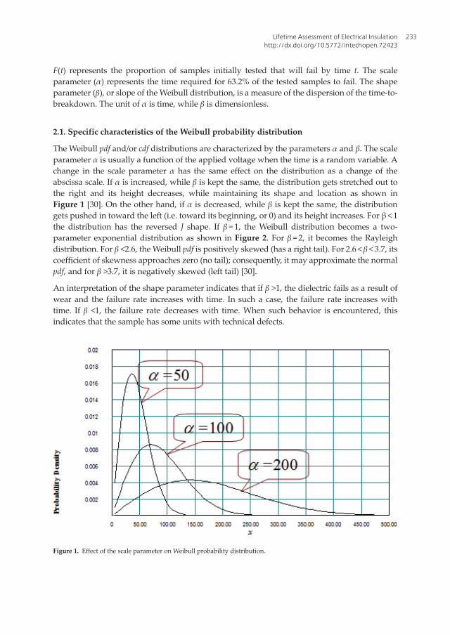
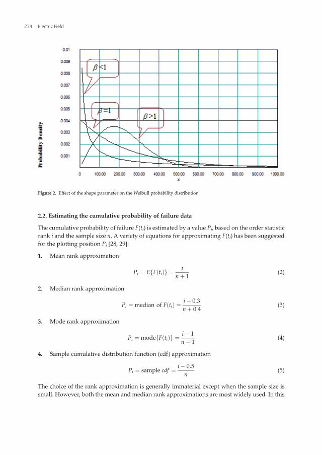
The Weibull pdf and/or cdf distributions are characterized by the parameters α and β. The scaleparameter α is usually a function of the applied voltage when the time is a random variable. Achange in the scale parameter α has the same effect on the distribution as a change of theabscissa scale. If α is increased, while β is kept the same, the distribution gets stretched out tothe right and its height decreases, while maintaining its shape and location as shown inFigure 1 [30]. On the other hand, if α is decreased, while β is kept the same, the distributiongets pushed in toward the left (i.e. toward its beginning, or 0) and its height increases. For β < 1the distribution has the reversed J shape. If β = 1, the Weibull distribution becomes a two-parameter exponential distribution as shown in Figure 2. For β = 2, it becomes the Rayleighdistribution. For β <2.6, the Weibull pdf is positively skewed (has a right tail). For 2.6 < β < 3.7, itscoefficient of skewness approaches zero (no tail); consequently, it may approximate the normalpdf, and for β >3.7, it is negatively skewed (left tail) [30].

An interpretation of the shape parameter indicates that if β >1, the dielectric fails as a result ofwear and the failure rate increases with time. In such a case, the failure rate increases withtime. If β <1, the failure rate decreases with time. When such behavior is encountered, thisindicates that the sample has some units with technical defects.

Figure 1. Effect of the scale parameter on Weibull probability distribution.

Lifetime Assessment of Electrical Insulationhttp://dx.doi.org/10.5772/intechopen.72423

233

2.2. Estimating the cumulative probability of failure data

The cumulative probability of failure F(ti) is estimated by a value Pi, based on the order statisticrank i and the sample size n. A variety of equations for approximating F(ti) has been suggestedfor the plotting position Pi [28, 29]:

1. Mean rank approximation

Pi ¼ E F tið Þf g ¼ inþ 1

(2)

2. Median rank approximation

Pi ¼ median of F tið Þ ¼ i� 0:3nþ 0:4

(3)

3. Mode rank approximation

Pi ¼ mode F tið Þf g ¼ i� 1n� 1

(4)

4. Sample cumulative distribution function (cdf) approximation

Pi ¼ sample cdf ¼ i� 0:5n

(5)

The choice of the rank approximation is generally immaterial except when the sample size issmall. However, both the mean and median rank approximations are most widely used. In this

Figure 2. Effect of the shape parameter on the Weibull probability distribution.

Electric Field234

work, the median rank approximation is used in estimating the probability of failure. Note thatthe median rank approximation is also known as Benard’s approximation.

2.3. Parameter estimation of Weibull distribution

The Weibull distribution parameters α and β are the variables that govern the characteristics ofthe Weibull pdf. Once the Weibull distribution has been selected to represent the failure data,the associated parameters can be determined from the experimental data. Weibull parameterscan be estimated graphically on a probability plotting paper [28–31] or analytically usingeither Least Squares (LS) or Maximum Likelihood (ML) estimation techniques. An overviewof these techniques [1–4] will be presented next.

2.4. Graphical technique

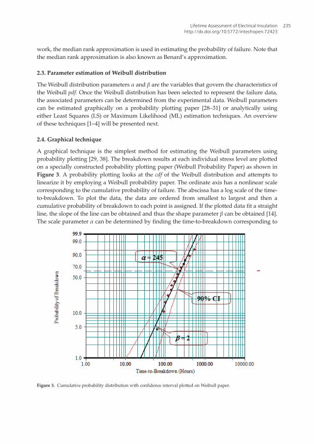
A graphical technique is the simplest method for estimating the Weibull parameters usingprobability plotting [29, 38]. The breakdown results at each individual stress level are plottedon a specially constructed probability plotting paper (Weibull Probability Paper) as shown inFigure 3. A probability plotting looks at the cdf of the Weibull distribution and attempts tolinearize it by employing a Weibull probability paper. The ordinate axis has a nonlinear scalecorresponding to the cumulative probability of failure. The abscissa has a log scale of the time-to-breakdown. To plot the data, the data are ordered from smallest to largest and then acumulative probability of breakdown to each point is assigned. If the plotted data fit a straightline, the slope of the line can be obtained and thus the shape parameter β can be obtained [14].The scale parameter α can be determined by finding the time-to-breakdown corresponding to

Figure 3. Cumulative probability distribution with confidence interval plotted on Weibull paper.


235

a cumulative probability of 63.2%. Using this simple, but time consuming approach, theparameters of the Weibull distribution can be determined. This procedure is repeated for eachstress level of the accelerated aging tests.

Estimating the parameters of the Weibull distribution by a graphical technique using a proba-bility plotting method has some shortfalls. A manual probability plotting is not always consis-tent in the results. Plotting a straight line through a set of points is a subjective procedure; itdiffers from person to person. In addition, the probability plot must be constructed for eachstress level. This, as a result, takes tremendous time and effort to plot the data. Furthermore,sufficient failures must be observed at each stress level, which is not always possible.

2.5. Least squares technique (LS)

The least squares technique is a linear regression estimation technique that fits a straight line toa set of data points, in an attempt to estimate the parameters associated with the straight lines.The parameters are estimated such that the sum of the squares of the vertical deviations fromthe points to the line is minimized according to [1–4]

J ¼XNi¼1

ea þ ebxi � yi� �2

¼ min ea;eb� �XNi¼1

ea þ ebxi � yi� �2

(6)

where eaand ebare the LS estimates of a and b, and N is the number of data points. To obtain eaand eb, the performance index J is differentiated with respect to a and b as shown below.

∂J∂ea ¼ 2

XNi¼1

ea þ ebxi � yi� �

(7)

∂J

∂eb ¼ 2XNi¼1


xi (8)

Setting Eqs. (7) and (8) equal to zero yields

XNi¼1


¼XNi¼1

eyi � yi� � ¼ �

XNi¼1

yi � eyi� � ¼ 0 (9)

XNi¼1

aþ bxi � yi� �

xi ¼XNi¼1

eyi � yi� �

xi ¼ �XNi¼1

yi � eyi� �xi ¼ 0 (10)

Solving Eqs. (9) and (10) simultaneously yields

ea ¼

PNi¼1

yi

N� eb

PNi¼1

xi

N(11)

Electric Field236

and

eb ¼

PNi¼1

xiyi �PNi¼1

xiPNi¼1

yi

N

PNi¼1

x2i �PNi¼1

xi

� �2

N

(12)

The least squares estimation technique is good for functions that can be linearized. Its calcula-tions are easy and straightforward, and the correlation coefficient provides a good measure ofthe goodness-of-fit of the chosen distribution. However, for some complex distributions, it isdifficult and sometimes impossible to implement.

2.6. Maximum likelihood estimation (MLE)

The maximum likelihood parameter estimation seeks to determine the parameters that maxi-mize the probability (likelihood) of the failure data. Statistically, the MLE is considered to bemore robust and yields estimators with good statistical properties. The MLE has the followingstatistical properties:

1. The ML estimators are consistent and asymptotically efficient.

2. The probability distribution of the estimators is asymptotically normal.

3. For small sample sizes, the ML estimators are considered to be more precise than thoseobtained by LS method. Moreover, the ML estimators can converge into a solution evenwith only one failure.

4. The MLE technique applies to most models and to different types of data.

5. The ML estimates are unique, and as the size of the sample increases, the estimatesstatistically approach the true values of the population.

The theory of the MLE method is described as follows: Let t be a continuous random variablerepresenting the time-to-breakdown and characterized by the two-parameter Weibull distri-bution with pdf:

f t;α;β� � ¼ β

α

� �tα

� �β�1

exp � tα

� �β" #

(13)

where α and β are unknown constant parameters which need to be estimated. For anexperiment with N independent observations, t1, t2, …, tN in a given sample, then the likeli-hood function associated with this sample is the joint density of the N random variables, andthus is a function of the unknown Weibull parameters (α, β). The likelihood function isdefined by [1–4]:


237

L t1; t2;⋯; tNjeα; eβ� �¼ L ¼

YNi¼1

f ti; eα; eβ� �¼YNi¼1

eβeα tieα� �~β�1

exp � tieα� �~β

" #(14)

The logarithmic likelihood function is given by

Λ ¼ lnL ¼XNi¼1

ln f ti; eα; eβ� �¼XNi¼1

lneβeα tieα� �~β�1

exp � tieα� �~β

!" #(15)

The parameter estimates eα; eβ� �are obtained by maximizing L or Λ which is much easier to

work with than L. The ML estimators are determined by taking the partial derivatives of Λ

with respect to eα and eβ set them to zero, that is, ∂Λ∂eα ¼ 0, ∂Λ

∂eβ ¼ 0, where,

∂Λ

∂eβ ¼XNi¼1

1eβ þXNi¼1

lntieα

� ��XNi¼1

tieα� �β

lntieα

� �� (16)

∂Λ∂eα ¼ �

XNi¼1

eβeα þeβeαXNi¼1

lntieα

� �~β

(17)

The resulting equations give the best estimates eβ and eα.1eβ ¼ � 1

N

XNi¼1

ln ti þXN

i¼1

tið Þ~β ln tiPNi¼1 tið Þ~β

(18)

eα ¼ 1N

XN

i¼1tið Þ~βÞ

� i 1=~βÞð�(19)

Eq. (18) is written in terms of eβ only, and can only be solved by an iterative technique, such as the

Newton-Raphson iterative technique. Once eβ, is obtained, eα can be determined using Eq. (19).

Although the methodology for the MLE is simple, the implementation is mathematicallyintense. The present high-speed computers, however, have made the obstacles of the mathe-matical complexity of the MLE an easy process. A specialized statistical commercial packageWeibull++ is used throughout this work to find the ML estimates of the Weibull distributionparameters [39].

2.7. Failure time percentiles

Once the Weibull distribution parameters are obtained, the failure time percentiles, tp, can bederived from Eq. (2) as follows (by substituting F(t; α, β) = p)

Electric Field238

tp ¼ eα � ln 1� pð Þ½ �1=~β (20)

where tp is the time-to-breakdown for which a sample will fail with a probability of failure p, andα ¼ L V;T; fð Þ is function of the applied stresses, (e.g. voltage, temperature, frequency, etc.). Ifp = 0.632, then tp = α, the scale parameter, or the life by which 63.2% of the samples will fail.Likewise, if p = 0.50, then tp=�t, the median life, or the life by which half of the samples will fail.

3. Life models

There are two approaches for studying the electrical breakdown and estimating the insulationlifetimes (under normal operating conditions) of polymeric insulating materials. One approachis based on phenomenological studies which require a complete understanding of the break-down mechanism. This approach requires physical and/or chemical tests to be performed onthe insulating material that may yield to the development of mathematical models functionalwith the lifetime. An example of this is relating the lifetime of the insulation to the length oftrees formed in the insulation bulk as a result of treeing mechanism [40]. The other widelyknown approach relies on a statistical analysis of failures that are attributed to the breakdownof the electrical insulation due to the presence of degrading stresses, such as electrical, thermal,and other environmental factors [6–36]. In this approach, the insulation life is determined bymeasuring the time-to-breakdown of identical specimens of the solid insulation subject to lifetests. Life tests, however, show that the times-to-breakdown are widely variable. This variationis best modeled by the Weibull probability distribution.

Conducting life tests at realistic working stresses is not possible due to the time constraint,given that most electrical insulation is expected to serve for several decades. Instead, break-down data are obtained, without paying much attention to the details of the breakdownmechanism, by conducting accelerated life (aging) tests in laboratory experiments so that theinsulation life is severely reduced [41, 42]. The main goal of life tests is to establish mathemat-ical models for the aging process and the stresses causing it [32–36]. The constants of thesemodels need to be estimated from life tests where the lifetimes at a variety of stress levels aremeasured. Once the constants are estimated, the life at any particular stress including normaloperating conditions can, in principle, be estimated.

3.1. Single-stress life models

Life models of single stress include the inverse power law and exponential law models for anelectrical stress, and the Arrhenius model for a thermal stress [32–34].

3.1.1. Life models for electrical stresses

An electrical stress is considered as one of the main factors causing deterioration of electricalinsulation. There are two empirical models that relate the test of an electrical stress to the


239

time-to-breakdown. One is the inverse power law model, and the second is the exponentiallaw model. The parameters of both models are obtained from experimental data taken atseveral different high voltage levels with other conditions unchanged. The electrical lifemodels mathematically describe the aging in a solid dielectric insulation that experiences anelectric stress [43]. The life models do not characterize the exact type of aging mechanismthat takes place. The life models are totally empirical and have no physical meaning otherthan defining the degradation rate as power or exponential. However, the models haveproven to fit reasonably well with experimental data.

3.1.1.1. Inverse power law

The inverse power law (IPL) model is one of the most frequently used in the aging studiesunder an electrical stress. The inverse power law model is given by:

L Vð Þ ¼ k V�n (21)

where L, the time-to-breakdown, is usually a Weibull scale parameter α at 63.2% probability, orany other percentile, V is the applied voltage, and k, n, are constants to be determined for thespecific tested material or device. The inverse power law is considered valid if the data beingplotted on a log–log graph fits a straight line [44].

3.1.1.2. Exponential law

The exponential law is also commonly used for lifetime calculations. The exponential model isgiven by:

L Vð Þ ¼ c exp �bVð Þ (22)

where L is the time-to-breakdown, V is the applied voltage, and c and b are constants to bedetermined from the experimental data. The exponential model is verified by plotting the datapoints on a semi-log graph. The model is considered valid if a straight line is obtained [44].

3.1.2. Life model for a thermal stress

The life of electrical insulation is seriously affected by a thermal stress. This effect can only berecognized by a thermal life test. The life of electrical insulation under a thermal stress isempirically expressed by the well-known Arrhenius equation. This equation describes thethermal aging of materials and shows the dependency of the chemical reaction rate as afunction of the temperature. The Arrhenius equation is given by [43]:

L Tð Þ ¼ A expBT

� �(23)

where L is the time-to-breakdown, T is the absolute temperature, and A, B are constants to bedetermined experimentally.

Electric Field240

3.2. Multi-stress life models

Multi-stress Life models were developed to predict the life of the insulation under combinedelectrical and thermal stresses. In general these models are limited to the common electricaland thermal aging stresses acting simultaneously [43]. Mainly, some models have empiricalnature such Simoni’s, Ramu’s, and Fallou’s [11, 12, 32–36]. These models account for theinteractions of electrical and thermal stresses by using a multiplicative law, in which the lifeunder a combined stress is related to the product of the single-stress lives. One possibleformula for this interaction can be manifested as the multiplication of the IPL model andArrhenius relationship, which is given by:

L V;Tð Þ ¼ KV�n expBT

� �(24)

which is considered to be the basis for both Simoni’s and Ramu’s electrical-thermal life models.Alternatively, the electrical exponential model is associated with the Arrhenius relationship.This can be expressed as:

L V;Tð Þ ¼ C exp AV þ BT

� �(25)

which constitutes the Fallou’s electrical-thermal life model.

Another probabilistic life model based on IPL was presented by Montanari et al. [34]. A briefoverview of the above mentioned electrical-thermal life models of Simoni, Ramu, Fallou, and theprobabilistic model by Montanari will be presented. The above models were developed for arelatively simple dielectric system involving polymer films or slabs. A variety of multi-stress lifetests have been also developed for more complex insulation systems, for example, cables androtatingmachines stator windings [16, 17]. However, lifetimemodels as a function of two ormorestresses are rarely derived due to excessive cost and time needed for collecting the failure data.

Regarding the frequency as an aging factor little research has been published in developingcombined electrical-thermal-frequency life models. In some works, high frequency sinusoidalvoltage was applied [41, 42]. The results of these works show that the frequency as an agingfactor that causes insulation deterioration. The effect of the frequency is modeled by relatingthe variation of the parameters of the life model to the frequency [41].

3.2.1. Simoni’s model

According to the Simoni’s model, the insulation life, in relative terms with respect to a refer-ence life determined by the absence of an electrical stress and at low temperature, is given by:

L V;Tð Þ ¼ toVVo

� �n

exp �BΔ1T

� �� (26)

where to is the time-to-breakdown at room temperature and V = Vo, Δ 1T

� � ¼ 1T � 1

To, and B and n

are constants which are determined experimentally.


241

3.2.2. Ramu’s model

The Ramu’s model is obtained from a multiplication of classical single-stress laws, and is givenby:

L V;Tð Þ ¼ K Tð Þ V½ ��n Tð Þ exp �BΔ1T

� �� (27)

where K Tð Þ ¼ exp K1 � K2Δ 1T

� �� , n Tð Þ ¼ exp n1 � n2Δ 1

T

� �� , K1, K2, n1, and n2 are constants.

Δ 1T

� �is the same as that defined for the Simoni’s model.

3.2.3. Fallou’s model

Fallou proposed a semi-empirical life model based on the exponential model for electricalaging:

L V;Tð Þ ¼ C exp AV þ BT

� �� (28)

where C, A, and B are electrical stress constants and must be determined experimentally fromtime-to-breakdown curves at constant temperatures.

3.2.4. Montanari’s probabilistic model

The probabilistic life model of combined electrical and thermal stresses by Montanari et al.relates the failure probability p to insulation life Lp. It is based on substituting the scaleparameter in the Weibull distribution with the life using the inverse power law. For a giventime-to-breakdown probability p, the probabilistic model is given by:

Lp V;Tð Þ ¼ Ls V=Vsð Þn � ln 1� pð Þ½ � 1=β Tð Þð Þ (29)

where Lp is a lifetime at probability p, Ls is a time-to-breakdown at reference voltage Vs, and βis the shape parameter.

3.3. Estimating life model constants

Eqs. (21) to (23) describe several mathematical models which relate insulation life to a singleaging stress, either voltage or temperature. Likewise, Eqs. (24) to (29) describe the electrical-thermal life models. In each model of the above life models, there are several parameters thatare needed to be estimated from life testing data. The parameters are estimated from life testswhere the lifetimes at a variety of stress levels are measured. Once the parameters are esti-mated, the life at any particular stress can, in principle, be estimated. This enables a method ofestimating the life at normal stress based on failure data collected from accelerated life tests.Traditionally, the parameters of life models are calculated either graphically or analyticallyusing graphical or regression analysis type methods.

Electric Field242

3.3.1. Graphical method

The graphical method for estimating the parameters of a life model involves generating twotypes of plots. First, the time-to-breakdown at each individual stress level is plotted on a proba-bility paper appropriate to the assumed life distribution (i.e. Weibull, Lognormal). The parame-ters at each stress level are then estimated from the plot. Once the parameters of the lifedistribution have been estimated at each stress level using probability plottingmethods, a secondplot is created in which a characteristic lifetime is plotted versus stress on a paper that linearizesthe assumed lifetime-stress relationship. For example, a log-log paper linearizes the inversepower law, a semi-log paper linearizes the exponential model, and a log-reciprocal linearizesthe Arrhenius relationship. The lifetime characteristic can be any percentile, such as 10% lifetime,the scale parameter, the mean lifetime, etc. The parameters of the lifetime-stress relationship arethen estimated from the second plot by solving for the slope and the intercept of the line [45].

In spite of the fact that the graphical method is simple and straightforward, the method suffersfrom some shortfalls such as:

• It is quite time consuming.

• The graphical method may fail in linearizing the lifetime-stress relationship when the dataare plotted on the special paper.

• In accelerated life tests with small data, the separation and individual plotting of the datato obtain the parameters increase the underlying error.

• The estimated parameters, that are assumed constant, are likely to vary when the test isrepeated. Confidence intervals on the estimated parameters cannot be established usingthe graphical methods.

3.3.2. Regression analysis

Calculating the parameters of a life model using regression analysis is relatively straightfor-ward. For most single-stress models, simple linear regression (SLR) is used to estimate theparameters. Similarly, multiple linear regression (MLR) is used for multi-stress models andcomplicated single-stress models. On the other hand, nonlinear regression methods areemployed in cases where life models contain thresholds below certain values where agingdoes not occur. These nonlinear models are much more difficult to analyze [40]. Therefore,non-statisticians do not usually use nonlinear regression. For this reason, most life modelsassume that the threshold is close to zero, permitting the use of conventional regressionanalysis. The MLR method first requires the life model to be linearized into a form such as:

y ¼ ao þ a1x1 þ a2x2 þ⋯þ akxk (30)

where y is a dependent variable (life, or a mathematical transformation of life), xk are indepen-dent stresses (or transformations of stresses or combinations of stresses), and ao, a1, a2,… ak arethe constants to be determined. The method of least squares can be used to estimate theregression constants in a MLR model. The least squares technique involves finding the values


243

of the constants that minimize the difference between the predicted lifetimes under a set ofstress conditions and the actual lifetime measures under the same conditions. By relating a“characteristic” life of the underlying probability distribution to the aging stress, a set ofmathematical equations can be used to calculate the parameters [45]. Each observation (xi1,xi2, …, xik, yi), satisfies the model in (30), or

yi ¼ ao þ a1xi1 þ a2xi2 þ⋯þ akxik

¼ ao þXkj¼1

ajxij i ¼ 1, 2,⋯, n(31)

The least squares function is:

J ¼Xni¼1

yi � ao �Xkj¼1

eajxij0@ 1A2

(32)

The function J is to be minimized with respect to ao, a1, a2, …, ak. The least squares estimates ofao, a1, a2, …, ak must satisfy:

∂J∂ao

ao, ao1, a2,⋯, ak ¼ �2Xni¼1

yi � eao �Xkj¼1

eajxij0@ 1A ¼ 0 (33)

∂J∂aj eao,eao1 ,ea2,⋯,eak

¼ �2Xni¼1

yi � eao �Xkj¼1

eajxij0@ 1Axij ¼ 0 j ¼ 1, 2,⋯, k (34)

Simplifying Eqs.(33) and (34), the following least squares normal equations are obtained:

neao þ ea1Xni¼1

xi1 þ ea2Xni¼1

xi2 þ⋯þ eakXni¼1

xik ¼Xni¼1

yi

eaoXni¼1

xi1 þ ea1Xni¼1

x2i2 þ ea2Xni¼1

xi1xi2 þ⋯þ eakXni¼1

xi1xik ¼Xni¼1

xi1yi

⋮ ⋮ ⋮ ⋮ ⋮ ⋮

eaoXni¼1

xik þ ea1Xni¼1

xikxi1 þ ea2Xni¼1

xikxi2 þ⋯þ eakXni¼1

x2ik ¼Xni¼1

xikyi

(35)

The solution to the k + 1 normal equations will be the least square estimators of the regressionparameters ao, a1, a2, …, ak of the multi-stress life model. The normal equations can be solvedby any method appropriate for solving a system of linear equations. Yet, it is much moreconvenient to solve the multiple linear regression problem using a matrix approach. For kparameters and n observations, the model relating the parameters to the dependent variableyn can be expressed in matrix notation as [45]:

Electric Field244

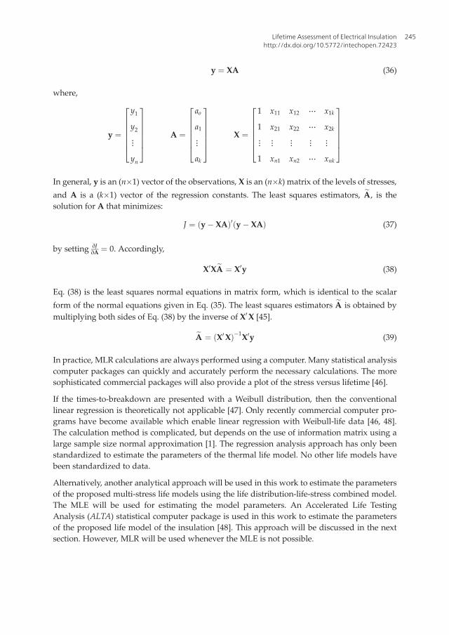
y ¼ XA (36)

where,

y ¼

y1

y2

⋮

yn

2666664

3777775 A ¼

ao

a1

⋮

ak

2666664

3777775 X ¼

1 x11 x12 ⋯ x1k

1 x21 x22 ⋯ x2k

⋮ ⋮ ⋮ ⋮ ⋮

1 xn1 xn2 ⋯ xnk

2666664

3777775In general, y is an (n�1) vector of the observations, X is an (n�k) matrix of the levels of stresses,

and A is a (k�1) vector of the regression constants. The least squares estimators, eA, is thesolution for A that minimizes:

J ¼ y� XAð Þ0 y� XAð Þ (37)

by setting ∂J∂A ¼ 0. Accordingly,

X0XeA ¼ X0y (38)

Eq. (38) is the least squares normal equations in matrix form, which is identical to the scalar

form of the normal equations given in Eq. (35). The least squares estimators eA is obtained bymultiplying both sides of Eq. (38) by the inverse of X0X [45].

eA ¼ X0Xð Þ�1X0y (39)

In practice, MLR calculations are always performed using a computer. Many statistical analysiscomputer packages can quickly and accurately perform the necessary calculations. The moresophisticated commercial packages will also provide a plot of the stress versus lifetime [46].

If the times-to-breakdown are presented with a Weibull distribution, then the conventionallinear regression is theoretically not applicable [47]. Only recently commercial computer pro-grams have become available which enable linear regression with Weibull-life data [46, 48].The calculation method is complicated, but depends on the use of information matrix using alarge sample size normal approximation [1]. The regression analysis approach has only beenstandardized to estimate the parameters of the thermal life model. No other life models havebeen standardized to data.

Alternatively, another analytical approach will be used in this work to estimate the parametersof the proposed multi-stress life models using the life distribution-life-stress combined model.The MLE will be used for estimating the model parameters. An Accelerated Life TestingAnalysis (ALTA) statistical computer package is used in this work to estimate the parametersof the proposed life model of the insulation [48]. This approach will be discussed in the nextsection. However, MLR will be used whenever the MLE is not possible.


245

4. Combined Weibull-life model

Three methods for estimating the parameters of accelerated life test models were presented inchapters two and three. First, the graphical method was illustrated using a probability plottingmethod for obtaining the parameters of the life distribution. The parameters of the life modelwere then estimated graphically by linearizing the model on a separate lifetime versus stressplot. However, not all life models can be linearized. Hence, instead of estimating the parame-ters of the life distribution and the life model graphically, an analytical technique based onleast squares was presented. However, the accuracy of the graphical method and LS estimationis affected by the probability rank approximation. Furthermore, estimating the parameters ofeach individual distribution leads to accumulation of uncertainties, depending on the numberof failures at each stress level. In addition, the slope (shape) parameters of each individualdistribution are rarely equal (common). Using the graphical method or the LS technique, onemust estimate a common shape parameter (usually the average) and repeat the analysis. Bydoing so, further uncertainties are introduced on the estimates, and these are uncertainties thatcannot be qualified [48].

On the other hand, combining the life distribution and the life model relationships in onestatistical model that describes both can be accomplished by including the life model into thepdf of the life distribution of failure data. Thus, the parameters of that combined model can beestimated using the complete likelihood function (L). Accordingly, a common shape parameter(β) is estimated from the combined model, thus eliminating the uncertainties of averaging theindividual shape parameters. All uncertainties are accounted for in the form of confidenceintervals that are quantifiable because they are obtained based on the overall model. Besides,the MLE technique is independent of any kind of probability ranks or a plotting method.Therefore, the MLE offers a very powerful method in estimating the parameters of life models[48].

The goal of the ML parameter estimation is to determine the parameters that maximize theprobability (likelihood) of the life data. Statistically, the method of the ML is considered to bemore robust and yields estimators with good statistical properties (unbiasedness, sufficiency,consistency, and efficiency). Due to its nature, the ML is a powerful tool in estimating theparameters of life models. In addition, the ML provides an efficient method for quantifyinguncertainty through confidence intervals.

4.1. Maximum likelihood estimation of combined Weibull-life model

For life data analysis, the two-parameter Weibull distribution pdf is commonly used to repre-sent the scatter of the failure data,

f t;α;β� � ¼ β

αtα

� �β�1

exp � tα

� �β" #

(40)

where t is the time-to-breakdown, α is the scale parameter (lifetime at 63.2%), and β is theshape parameter or the slope of the Weibull cumulative distribution. The parameters of the life

Electric Field246

model can be statistically calculated by combining the life model to the Weibull distribution.For example, the combined Weibull-life model can be derived by setting the scale parameterα=L(V) for the electrical life model, or α=L(V,T) for the electrical-thermal multi-stress life model[13]. The maximum likelihood parameter estimation of combined Weibull-life model will bepresented in this chapter for both single-stress and multi-stress life models. The inverse powerlaw (IPL) of the electrical life model and exponential-Arrhenius of the electrical-thermal lifemodel will be used as examples to show the procedure for deriving the parameters of thecombined Weibull-life model.

4.2. Weibull-inverse power law electrical life model

The combined Weibull-IPL model can be derived by setting α ¼ L Vð Þ ¼ kV�n, yielding thefollowing Weibull pdf,

f t;Vð Þ ¼ βKVn KVntð Þβ�1 exp � KVntð Þβ� �

(41)

where K = 1/k. This is a three-parameter model (K, β, n) where the parameters can be deter-mined experimentally using life test data.

4.2.1. Parameter estimation of Weibull-IPL model using MLE method

Substituting the IPL electrical life model into the Weibull-Log-Likelihood function yields (Λ)yields:

Λ ¼XMj¼1

XNi¼1

ln eβ eKVenj eKVenj ti� �~β�1

exp � eKVenj ti� �~β� ��

(42)

where M is the number of electrical life test groups; N is the number of times-to-breakdown in

jth life test; Vj is the jth life voltage; ti is the ith time-to-breakdown in the jth group; eβ is an

estimate of the Weibull shape parameter; eK = 1/k, k is the IPL Parameter; en is the secondparameter of IPL.

The ML estimates of the parameters can be found by solving for eβ, eK, en such that [45].

∂Λ

∂eβ ¼ 0,∂Λ

∂eK ¼ 0,∂Λ∂en ¼ 0:

where,

∂Λ

∂eβ ¼XMj¼1

XNi¼1

1eβ þXMj¼1

XNi¼1

ln eKVenj ti� ��XMj¼1

XNi¼1

eKVenj ti� �~βln eKVenj ti� �

(43)

∂Λ

∂eK ¼XMj¼1

XNi¼1

eβeK �eβeKX

M

i¼1

XNi¼1

eKVenj ti� �~β(44)


247

∂Λ∂en ¼ eβXM

j¼1

XNi¼1

ln Vj� �� eβXM

j¼1

XNi¼1

ln Vj� � eKVenj ti� �~β

(45)

4.3. Electrical-thermal life model

In this dissertation, a new electrical-thermal relationship has been proposed for predicting thelifetime of magnet wire insulation at service conditions when the voltage and temperature arethe accelerated stresses in a test. This new combined model is given by:

L V;Tð Þ ¼ C expAVþ BT

� �(46)

where L is the lifetime at 63.2% probability of breakdown; V is the voltage; T is the temperature;C, A, and B: are constants to be estimated by analyzing the joint voltage-temperature life data.

The proposed lifetime relationship can be linearized by finding the natural logarithm of bothsides of Eq. (46). A family of linear curves can be obtained by plotting the lifetime versus eitherof the stresses, Vor T, and keeping the other one constant. In this case, the constant B representsthe slope of the linearized Arrhenius equation when the voltage is constant, and A representsthe slope of the exponential electrical function model when the temperature is constant [45].

Considering that the lifetime is a random variable, the above model can be converted to aprobabilistic model by setting the scale parameter α of the Weibull distribution equals to L(V,T)of Eq. (46). Therefore, assuming the time-to-breakdown of the electrical insulation, undercombined electrical and thermal stresses, is statistically distributed according to a Weibulldistribution, then the Weibull pdf can be written as [45]

f t;V;Tð Þ ¼ βC

exp � AVþ BT

� �tCexp � A

Vþ BT

� �� β�1

exp � tC

exp � AVþ BT

� �� β

(47)

This Weibull pdf will be used to estimate the parameters of the electrical-thermal life model.

4.3.1. Parameter estimation of Weibull-electrical-thermal life model using MLE

The combined Weibull-electrical-thermal model has four parameters to be estimated using thejoint voltage-temperature life data. Using the MLE method, the log-likelihood function of thecombined Weibull-electrical-thermal pdf is given by [45]:

Λ¼ ln Lð Þ ¼XMj¼1

XPi¼1

XNl¼1

lneβeC exp �

eAVi

þeBTj

!tleC exp �

eAVi

þeBTj

! !~β�1

exp � tleC exp �eAVi

þeBTj

! !~β24 35

(48)

whereM is the number of thermal life test groups at voltage Vi; P is the number of electrical lifetest groups at temperature Tj; N is the number of times-to-breakdown in the jith electrical-thermal life test; Vi is the i

th life voltage at the jth life temperature; Tj: is the jth life temperature at

the ith life voltage; tl is the lth time-to-breakdown in the jith group; eβ is the estimate of the

Electric Field248

Weibull shape parameter; eC is an estimate of a parameter of the combined E-T life model; eA is

an estimate of a parameter of the combined E-T life model; eB is an estimate of a parameter ofthe combined E-T life model.

The parameter estimates eβ; eC; eA; eB� �can be found by solving:

∂Λ

∂eβ ¼ 0,∂Λ

∂eC ¼ 0,∂Λ

∂eA ¼ 0,∂Λ

∂eB ¼ 0:

where,

∂Λ

∂eβ ¼XMj¼1

XPi¼1

XNl¼1

1eβ þXMj¼1

XPi¼1

XNl¼1

lntleC exp �

eAVi

þeBTj

! !�

XMj¼1

XPi¼1

XNl¼1

tleC exp �eAVi

þeBTj

! !~β

lntleC exp �

eAVi

þeBTj

! ! (49)

∂Λ

∂eC ¼XMj¼1

XPi¼1

XNl¼1

�eβeC þ

eβeCXM

j¼1

XPi¼1

XNl¼1

tleC exp �eAVi

þeBTj

! !~β

(50)

∂Λ

∂eA ¼XMj¼1

XPi¼1

XNl¼1

eβ �1Vi

� �þXMj¼1

XPi¼1

XNl¼1

βVi

� �:

tleC exp � AVi

þeBTj

! !~β

(51)

∂Λ

∂eB ¼XMj¼1

XPi¼1

XNl¼1

eβ �1Tj

� �þXMj¼1

XPi¼1

XNl¼1

βTj

� �:

tleC exp � AVi

þeBTj

! !~β

(52)

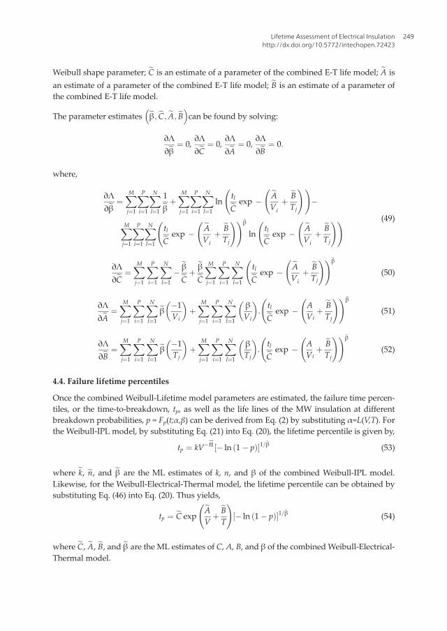
4.4. Failure lifetime percentiles

Once the combined Weibull-Lifetime model parameters are estimated, the failure time percen-tiles, or the time-to-breakdown, tp, as well as the life lines of the MW insulation at differentbreakdown probabilities, p = Fp(t;α,β) can be derived from Eq. (2) by substituting α=L(V,T). Forthe Weibull-IPL model, by substituting Eq. (21) into Eq. (20), the lifetime percentile is given by,

tp ¼ kV�en � ln 1� pð Þ½ �1=~β (53)

where ek, en, and eβ are the ML estimates of k, n, and β of the combined Weibull-IPL model.Likewise, for the Weibull-Electrical-Thermal model, the lifetime percentile can be obtained bysubstituting Eq. (46) into Eq. (20). Thus yields,

tp ¼ eC expeAVþeBT

!� ln 1� pð Þ½ �1=~β (54)

where eC, eA, eB, and eβ are the ML estimates of C, A, B, and β of the combinedWeibull-Electrical-Thermal model.


249

Nomenclature

ALTA accelerated life testing analysis

α Weibull scale parameter

β Weibull shape parameter

cdf cumulative distribution function

IPL inverse power law

LS least squares

L lifetime

ML maximum likelihood

MLE maximum likelihood estimation

MLR multiple linear regression

pdf probability density function

SLR simple linear regression

t time-to-breakdown

T absolute temperature

V applied voltage

Vs reference voltage

Author details

Eyad A. Feilat

Address all correspondence to: [email protected]

The University of Jordan, Amman, Jordan

References

[1] Lawless JF. Statistical Models and Methods for Lifetime Data. 2nd ed. New York: JohnWiley & Sons; 2003. DOI: 10.1002/9781118033005

[2] Nelson WB. Accelerated Testing: Statistical Models, Test Plans, and data Analyses. NewYork: John Wiley & Sons; 2008. DOI: 10.1002/9780470316795

[3] Mann RN, Schafer RE, Singpurwalla ND. Methods for Statistical Analysis of Reliabilityand Life Data. New York: John Wiley & Sons; 1974

Electric Field250

[4] Meeker WQ, Escobar LA. Statistical Methods for Reliability Data. New York: John Wiley& Sons; 1998

[5] Occhini E. A statistical approach to the discussion of the dielectric strength in electriccables. IEEE Transactions on Power Apparatus and Systems. 1971;90:2671-2678. DOI:10.1109/TPAS.1971.292920

[6] Feilat EA, Grzybowski S, Knight P, Doriott L. Breakdown and aging behavior of com-posite insulation system under DC and AC high voltages. WSEAS Transactions on Cir-cuits and Systems. 2005;4:780-787

[7] Grzybowski S, Dobroszewski R, Grzegorski E: Accelerated endurance tests of polyethyleneinsulated cables. In: Proceedings of the 3rd International Conference on Dielectric Mate-rials, Measurements and Applications; 10-13 September 1979; Birmingham, UK. p. 120–123

[8] Cacciari M, Montanari GC. Optimum design of life tests for insulating materials, systemsand components. IEEE Transactions on Electrical Insulation. 1991;26:1112-1123. DOI:10.1109/14.108148

[9] Mazznti G, Montanari GC, Simoni L. Insulation characterization in multistress conditionsby accelerated life tests: an application to XLPE and EPR for high voltage cables. IEEEElectrical Insulation Magazine. 1997;13:24-34. DOI: 10.1109/57.637151

[10] Björklund A, Siberg H, Paloniemi P. Accelerated ageing of a partial discharge resistantenameled round wire. In: Proceedings of the Electrical Electronics Insulation Conference;18-21 September 1995; Rosemont, Illinois. pp. 417–419

[11] Fallou B, Burguiere C, Morel JF. First approach on multiple stress accelerated life testing ofelectrical insulation. In: 1979 Annual Report of CEIDP; Pennsylvania, USA. pp. 621–628

[12] Ramu TS. On the estimation of life of power apparatus insulation under combinedelectrical and thermal stress. IEEE Transactions on Electrical Insulation. 1985;20:70-78.DOI: 10.1109/TEI.1985.348759

[13] Feilat EA, Grzybowski S, Knight P. Multiple stress aging of magnet wire by high frequencyvoltage pulses and high temperatures. In: Conference Records of the 2000 IEEE Interna-tional Symposium on Electrical Insulation (ISEI2000); 2–05-04-2000; CA, USA. pp. 157–160

[14] Grzybowski S, Feilat EA, Knight P, Doriott L. Breakdown voltage behavior of PETthermoplastics at DC and AC Voltages. In: Proceedings of the IEEE SoutheastCon99; 25-28 March 1999; Lexington, Kentucky, USA. pp. 284–287

[15] Grzybowski S, Feilat EA, Knight P, Doriott L. Accelerated aging tests on magnet wiresunder high frequency pulsating voltage and high temperature. In: Annual Report of the1999 Conference on Electrical Insulation and Dielectric Phenomena, (CEIDP99); 17-21 Octo-ber 1999; Austin, Texas, USA. pp. 555–558

[16] Kim J, Kim W, Park H-S, Kang J-W. Lifetime assessment for oil-paper insulation usingthermal and electrical multiple degradation. Journal of Electrical Engineering and Tech-nology. 2017;12:840-845. DOI: 10.5370/JEET.2017.12.2.840

[17] Li Y, Tian M, Lei Z, Song J, Zeng J, Lin L, Li Y. Breakdown performance and electricalaging life model of EPR used in coal mining cables. In: Proceedings of the IEEE


251

International Conference on High Voltage Engineering and Application (ICHVE); 19-22September 2016; Chengdu, China

[18] Maussion P, Picot A, Chabert M, Malec D. Lifespan and aging modeling methods forinsulation systems in electrical machines: a Survey. In: Proceedings of the 2nd IEEEWorkshop on Electrical Machines Design, Control and Diagnostics (WEMDCD’15); 26-27 March 2015; Turin, Italy

[19] Akolkar SM, Kushare BE. Remaining life assessment of power transformer. Journal ofAutomation and Control. 2014;2:45-48. DOI: 10.12691/automation-2-2-2

[20] Kerimli GM. On the mechanism of electrical aging of polymer insulation materials.Surface Engineering and Applied Electrochemistry. 2014;50:485-490. DOI: 10.3103/S1068375514060052

[21] Lahoud N, Faucher J, Malec D, Maussion P. Electrical aging of the insulation of lowvoltage machines: model definition and test with the design of experiments. IEEE Trans-actions on Industrial Electronics. 2013;60:4147-4155. DOI: 10.1109/TIE.2013.2245615

[22] Nasrat LS, Kassem N, Shukry N. Aging effect on characteristics of oil impregnated insula-tion paper for power transformers. Engineering. 2013;5:1-7. DOI: 10.4236/eng.2013.51001

[23] Koltunowicz TL, Cavallini A, Djairam D, Montanari GC, Smit JJ. The influence of squarevoltage waveforms on transformer insulation break down voltage. In: 2011 Annual ReportConference on Electrical Insulation and Dielectric Phenomena; 16–19-10-2011; Mexico

[24] Mazzanti G, Montanari GC, Dissado LA. Electrical aging and life models: the role ofspace charge. IEEE Transactions on Dielectrics and Electrical Insulation. 2005;12:876-890.DOI: 10.1109/TDEI.2005.1522183

[25] Liao RJ, Liang SW, Sun CX, Yang LJ, Sun HG. A comparative study of thermal aging oftransformer insulation paper impregnated in natural ester and in mineral oil. EuropeanTransactions on Electrical Power. 2010;20:518-523. DOI: 10.1002/etep.336

[26] Montanari GC, Mazzanti G, Simoni L. Progress in electrothermal life modeling of electri-cal insulation during the last decades. IEEE Transactions on Dielectrics and ElectricalInsulation. 2002;9:730-745. DOI: 10.1109/TDEI.2002.1038660

[27] Kaufhold M, Aninger H, Berth M, Speck J, Eberhardt M. Electrical stress and failuremechanism of the winding insulation in PWM-inverter fed low-voltage induction motors.IEEE Transactions on Industrial Electronics. 2000;47:396-402. DOI: 10.1109/41.836355

[28] Stone GC. The application of Weibull statistics to insulation aging tests. IEEE Transac-tions on Electrical Insulation. 1979;14:233-239. DOI: 10.1109/TEI.1979.298226

[29] Fothergill JC. Estimating the cumulative probability of failure data points to be plotted onWeibull and other probability papers. IEEE Transactions on Electrical Insulation. 1990;25:489-4992. DOI: 10.1109/14.55721

[30] Reliability Engineering Resources[Internet]. Available from: http://www.weibull.com

[31] Jacquelin J. Inference of sampling on Weibull parameter estimation. IEEE Transactionnson Dielectrics and Electrical Insulation. 1996;3:809-816. DOI: 10.1109/94.556564

Electric Field252

[32] Cygan P, Laghari JR. Models for insulation aging under electrical and thermal multistress.IEEE Transactions on Electrical Insulation. 1990;25:923-934. DOI: 10.1109/14.59867

[33] Laghari JR. Complex electrical thermal and radiation aging of dielectric films. IEEETransactions on Electrical Insulation. 1993;28:777-788. DOI: 10.1109/14.237741

[34] Montanari GC, Simoni L. Aging phenomenology and modeling. IEEE Transactions onElectrical Insulation. 1993;28:755-776. DOI: 10.1109/14.237740

[35] Gjaerde AC. Multifactor ageing models-origin and similarities. IEEE Electrical InsulationMagazine. 1997;13:6-13. DOI: 10.1109/CEIDP.1995.483610

[36] Montanari GC, Cacciari M. A probabilistic insulation life model for combined thermal-electrical stresses. IEEE Transactions on Electrical Insulation. 1985;20:519-522. DOI:10.1109/TEI.1985.348776

[37] Dissado LA, Fothergill JC, Wolfe SV, Hill RM. Weibull statistics in dielectric breakdown;theoretical basis, applications and implications. IEEE Transactions on Electrical Insula-tion. 1984;19:227-233. DOI: 10.1109/TEI.1984.298753

[38] Gibbons DI, Vance LC. A simulation study of estimators for the 2-parameter Weibulldistribution. IEEE Transactions on Reliability. 1981;30:61-66. DOI: 10.1109/TR.1981.5220965

[39] Weibull++ Life Data Analysis Reference, Version 11. Arizona, USA: ReliaSoft’s; 2017

[40] Eichhorn RM. Treeing in solid extruded electrical insulation. IEEE Transactions on Elec-trical Insulation. 1977;12:2-8. DOI: 10.1109/TEI.1977.298001

[41] Kachen W, Laghari JR. Determination of aging-model constants under high frequencyand high electric fields. IEEE Transactions on Dielectrics and Electrical Insulation. 1994;6:1034-1038. DOI: 10.1109/94.368660

[42] Cygan P, Krishnakumar B, Laghari JR. High field electrical and thermal aging of polypro-pylene films. In: Conference Record of the 1988 IEEE International Symposium on ElectricalInsulation; 5-8 June 1988; Boston, MA, USA. pp. 188–191. DOI: 10.1109/ELINSL.1988.13901

[43] Grzybowski S, Bandaru S: Effect of multistress on the lifetime characteristics of magnetwires used in flyback transformer. In: Conference Record of the IEEE International Sym-posium on Electrical Insulation; 19-22 September 2004; Indianapolis, IN, USA

[44] Feilat E A, Grzybowski S, Knight P. Electrical aging models for fine gauge magnet wireenamel of flyback transformer. In: Proceedings of the IEEE Southeast Con 2000; 7-9 April2000; Nashville, TN, USA. pp. 146–149

[45] Feilat EA. Lifetime characteristics of magnet wires under high frequency pulsating volt-age and high temperature [Thesis]. Mississippi State: Mississippi State University; 2000

[46] SAS/STAT Guide for Personal Computers, Version 6, Chapter 21. The LIFEREG Proce-dure. SAS Institute, 1987

[47] Draper NR, Smith H. Applied Regression Analysis. John Wiley & Sons; 2014. DOI:10.1002/9781118625590

[48] Accelerated Life Testing Analysis, Version 11. Tucson, Arizona, USA. ReliaSoft’s: 2017


253

lifetime assessment of electrical insulation

Documents