lifetime monitoring of wind turbines - lund...
TRANSCRIPT

ISSN 0280-5316 ISRN LUTFD2/TFRT--5759--SE
Lifetime Monitoring of Wind Turbines
Lars Nilsson
Department of Automatic Control Lund University November 2005


Document name MASTER THESIS Date of issue November 2005
Department of Automatic Control Lund Institute of Technology Box 118 SE-221 00 Lund Sweden Document Number
ISRNLUTFD2/TFRT--5759--SE Supervisor Rolf Johansson at Automatic Control in Lund Florian Krug at General Electric Global Research in München.
Author(s) Lars Nilsson
Sponsoring organization
Title and subtitle Lifetime Monitoring of Wind Turbines (Livstidsövervakning av vindkraftverk)
Abstract The aim of this thesis was to design and implement a lifetime monitoring system for a GE Energy wind turbine. Monitoring the loads on the main components of a wind turbine makes it possible to keep the lifetime of the components monitored. This information can be used to enable more flexible planning of a wind turbine’s maintenance. Knowing the estimated remaining lifetime makes it possible to change the components before they break. This increases both the security and availability of the wind turbine. The information from the lifetime monitoring system could possibly also be used directly by the wind turbine’s main controller in order to optimize the operation of the wind turbine regarding its components lifetime and the turbine’s energy capture. Several load-cycle counting methods were investigated and compared to each other and the rainflow counting method was found to be the most suitable. It was adapted, implemented and tested on a PLC (Programmable Logical Controller) mounted to a HITL (Hardware In The Loop) real-time simulation system that simulated the behavior of a GE 1.5 s/sl wind turbine. A method for calculating the fatigue, using the result from the rainflow counting, was implemented. The whole monitoring system was designed and implemented to work online, i.e., continuously calculating and displaying the lifetime of the monitored components. In order to realize an online rainflow counter, a novel approach for classification of the data-series was developed. A prototype of the system was installed on a GE Energy wind turbine in Salzbergen, Germany. Several tests were here performed in order to validate the system and to compare the simulated results with the measured results.
Keywords
Classification system and/or index terms (if any)
Supplementary bibliographical information ISSN and key title 0280-5316
ISBN
Language English
Number of pages 83
Security classification
Recipient’s notes
The report may be ordered from the Department of Automatic Control or borrowed through:University Library, Box 3, SE-221 00 Lund, Sweden Fax +46 46 222 42 43


Acknowledgment
This work was carried out for the Department of Automatic Control at the Lund In-stitute of Technology, Sweden, in cooperation with General Electric Global Research inGarching, Munich, Germany.
First of all I would like to thank Professor Rolf Johansson from the Department ofAutomatic Control at the Lund Institute of Technology, for his helpful advices and tipsfor my master thesis.
Thanks, to my supervisor Dr.-Ing. Florian Krug, GE Global Research, for believingin this project and always giving me the necessary support.
I would also like to thank Dipl.-Ing. Christian Schram for his encouragement and forthe very helpful technical brainstorming sessions.
A special thank you to Wilhelm Feichter, GE Global Research, for the outstandingcollaboration and all the technical help.
Thanks, to Thorsten Honekamp for his useful help in questions regarding rainflowcounting and classification.
Thanks, to Friedrich Loh, GE Energy, for his assistance during the prototype instal-lation in Salzbergen.
Thanks, to all my colleagues at GE Global Research for the friendship, the inspiringatmosphere, and the pleasant coffee-breaks.
Last, but not least, I would like to thank my girlfriend Natalie Terenya for her un-yielding support and love.
iii


Contents
1 Introduction 1
1.1 Motivation . . . . . . . . . . . . . . . . . . . . . . . . . . . . . . . . . . . 11.2 Aim . . . . . . . . . . . . . . . . . . . . . . . . . . . . . . . . . . . . . . 21.3 Outline . . . . . . . . . . . . . . . . . . . . . . . . . . . . . . . . . . . . . 2
I Methods 3
2 Cycle Counting 5
2.1 Approach Analysis . . . . . . . . . . . . . . . . . . . . . . . . . . . . . . 52.2 Rainflow Counting . . . . . . . . . . . . . . . . . . . . . . . . . . . . . . 5
2.2.1 General . . . . . . . . . . . . . . . . . . . . . . . . . . . . . . . . 52.2.2 Recursive Algorithm . . . . . . . . . . . . . . . . . . . . . . . . . 62.2.3 Non-Recursive Algorithm . . . . . . . . . . . . . . . . . . . . . . . 82.2.4 Rainflow Matrix . . . . . . . . . . . . . . . . . . . . . . . . . . . . 92.2.5 Residual . . . . . . . . . . . . . . . . . . . . . . . . . . . . . . . . 122.2.6 Processing Succeeding Sequences . . . . . . . . . . . . . . . . . . 152.2.7 Preprocessing Functions . . . . . . . . . . . . . . . . . . . . . . . 15
2.3 Conclusions . . . . . . . . . . . . . . . . . . . . . . . . . . . . . . . . . . 19
3 Fatigue Analysis 21
3.1 General . . . . . . . . . . . . . . . . . . . . . . . . . . . . . . . . . . . . 213.2 Damage Calculation . . . . . . . . . . . . . . . . . . . . . . . . . . . . . 223.3 Conclusions . . . . . . . . . . . . . . . . . . . . . . . . . . . . . . . . . . 24
4 Wind Turbine Setup 27
4.1 Structure . . . . . . . . . . . . . . . . . . . . . . . . . . . . . . . . . . . 274.2 Sensors . . . . . . . . . . . . . . . . . . . . . . . . . . . . . . . . . . . . . 28
5 Hardware Setup 33
5.1 Hardware In The Loop . . . . . . . . . . . . . . . . . . . . . . . . . . . . 335.2 Development Setup . . . . . . . . . . . . . . . . . . . . . . . . . . . . . . 355.3 Prototype Setup . . . . . . . . . . . . . . . . . . . . . . . . . . . . . . . . 35
v

Contents
5.4 Conclusions . . . . . . . . . . . . . . . . . . . . . . . . . . . . . . . . . . 38
6 Developed Software 39
6.1 Development Environment . . . . . . . . . . . . . . . . . . . . . . . . . . 396.2 Program Organization Units . . . . . . . . . . . . . . . . . . . . . . . . . 396.3 Design . . . . . . . . . . . . . . . . . . . . . . . . . . . . . . . . . . . . . 40
6.3.1 First Design Approach . . . . . . . . . . . . . . . . . . . . . . . . 406.3.2 Second Design Approach . . . . . . . . . . . . . . . . . . . . . . . 41
6.4 Developed POU’s . . . . . . . . . . . . . . . . . . . . . . . . . . . . . . . 426.4.1 Program Lifetime_calc_main . . . . . . . . . . . . . . . . . . . . 426.4.2 Function Block Filter_max_min_REAL . . . . . . . . . . . . . . 436.4.3 Function Block Filter_max_min_INT . . . . . . . . . . . . . . . 446.4.4 Function Block Filter_max_min_REAL_v2 . . . . . . . . . . . 446.4.5 Function Block Rfc . . . . . . . . . . . . . . . . . . . . . . . . . . 446.4.6 Function Block Rfc_v2 . . . . . . . . . . . . . . . . . . . . . . . . 446.4.7 Function Block Damage_calc . . . . . . . . . . . . . . . . . . . . 466.4.8 Function Block Matrix_2_file . . . . . . . . . . . . . . . . . . . . 46
6.5 Developed GUI’s . . . . . . . . . . . . . . . . . . . . . . . . . . . . . . . 466.6 Matlab Implementation . . . . . . . . . . . . . . . . . . . . . . . . . . . . 466.7 Real-time Requirements . . . . . . . . . . . . . . . . . . . . . . . . . . . 476.8 Conclusions . . . . . . . . . . . . . . . . . . . . . . . . . . . . . . . . . . 48
II Results and Validation 49
7 Simulation using HITL 51
8 Calculations for a Measurement 59
III Conclusions and Perspectives 63
9 Summary 65
10 Quality Assessments 67
11 Future Work 69
Bibliography 70
vi

List of Figures
2.1 Example of how recursive rainflow counting works . . . . . . . . . . . . . 7
2.2 Cycles found by the rainflow method (marked with circles) and the re-maining residual . . . . . . . . . . . . . . . . . . . . . . . . . . . . . . . . 8
2.3 Hystereses cycles in the stress-strain plane . . . . . . . . . . . . . . . . . 9
2.4 Rainflow counting example, steps 1 - 3 . . . . . . . . . . . . . . . . . . . 10
2.5 Rainflow counting example, steps 4 - 6 . . . . . . . . . . . . . . . . . . . 11
2.6 Rainflow matrix defined in two ways . . . . . . . . . . . . . . . . . . . . 12
2.7 Residual’s part in rainflow counting when several succeeding data seriesare to be taken into account . . . . . . . . . . . . . . . . . . . . . . . . . 13
2.8 Rainflow counting of the residual . . . . . . . . . . . . . . . . . . . . . . 14
2.9 Description of a high and low resolution rainflow matrix . . . . . . . . . 17
3.1 Example of a SN-curve . . . . . . . . . . . . . . . . . . . . . . . . . . . . 22
4.1 Model of a GE 1.5s/sl wind turbine [GEWE04] . . . . . . . . . . . . . . 27
4.2 Cross section of a wind turbine blade describing how the pitch-angle, theflap direction, and the edge direction should be interpreted . . . . . . . . 29
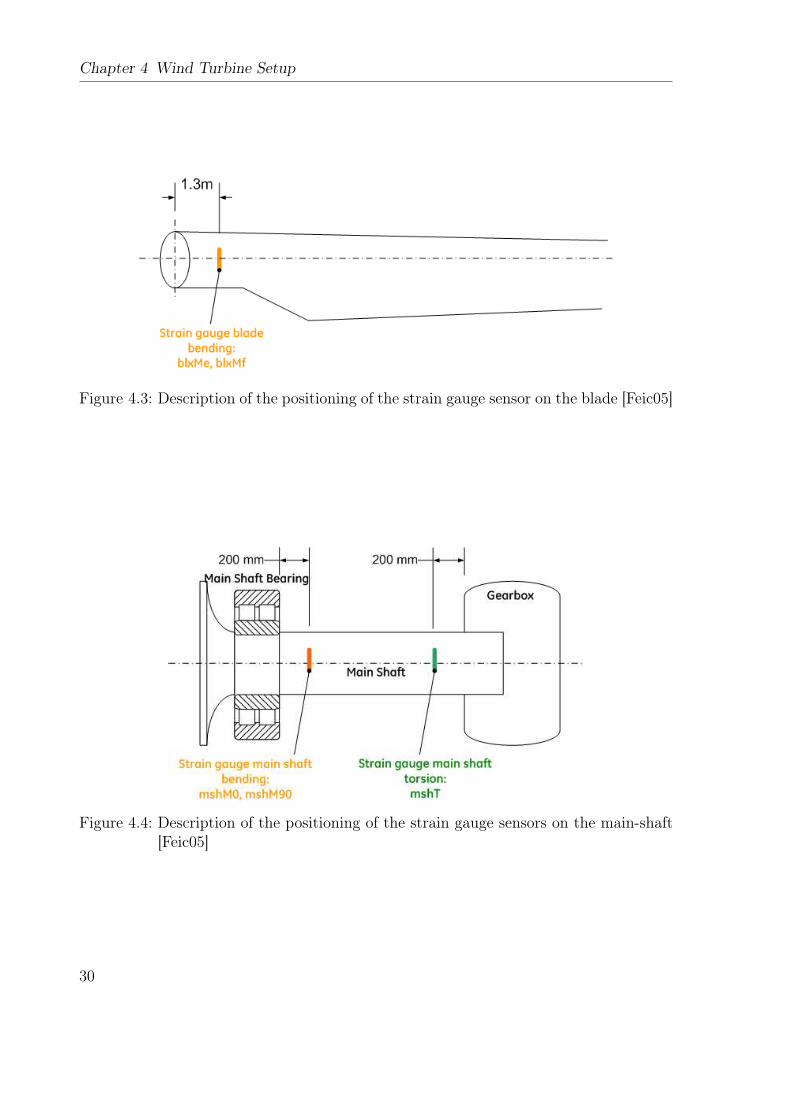
4.3 Description of the positioning of the strain gauge sensor on the blade[Feic05] . . . . . . . . . . . . . . . . . . . . . . . . . . . . . . . . . . . . . 30
4.4 Description of the positioning of the strain gauge sensors on the main-shaft [Feic05] . . . . . . . . . . . . . . . . . . . . . . . . . . . . . . . . . 30
4.5 Description of the positioning of the strain gauge sensors on the tower . . 31
5.1 Block diagram of an embedded system connected to a HITL-simulator . . 33
5.2 HITL system architecture [GEGR04] . . . . . . . . . . . . . . . . . . . . 34
5.3 System overview of the development setup [Feic05] . . . . . . . . . . . . . 36
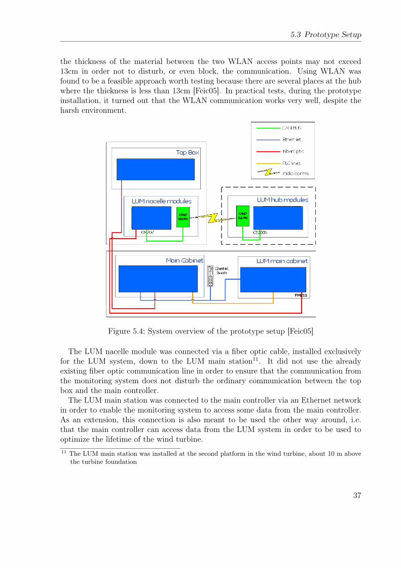
5.4 System overview of the prototype setup [Feic05] . . . . . . . . . . . . . . 37
6.1 Software flowchart for the first design approach . . . . . . . . . . . . . . 40
6.2 Software flowchart for the second design approach . . . . . . . . . . . . . 42
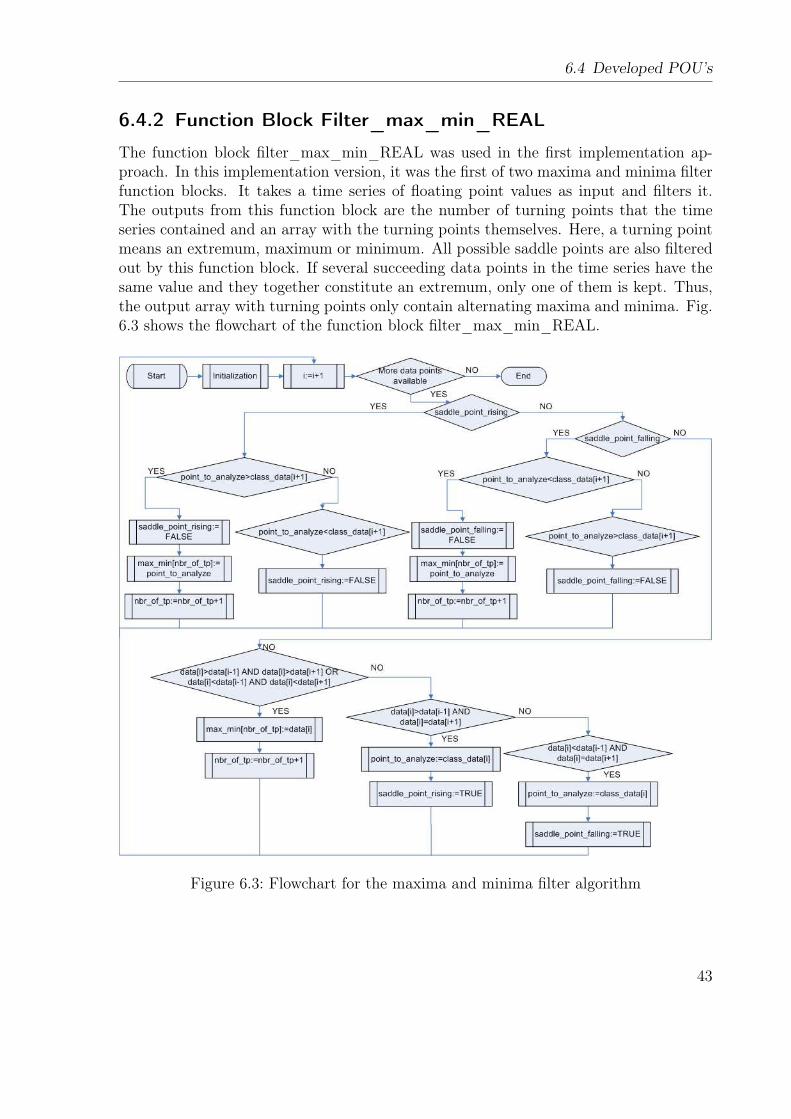
6.3 Flowchart for the maxima and minima filter algorithm . . . . . . . . . . 43
6.4 Flowchart for the rainflow algorithm . . . . . . . . . . . . . . . . . . . . 45
vii

List of Figures
6.5 GUI showing the total damage that has been calculated for the monitoredsensors . . . . . . . . . . . . . . . . . . . . . . . . . . . . . . . . . . . . . 47
7.1 The four time frames obtained from the simulation . . . . . . . . . . . . 527.2 Development of the high resolution rainflow matrix, for the blxMe sensor,
during four time frames . . . . . . . . . . . . . . . . . . . . . . . . . . . 547.3 High resolution rainflow matrix calculated by the monitoring system, us-
ing internal classification, for a time frame from the blxMe sensor . . . . 557.4 Rainflow matrix calculated with the signal processing tool FAMOS, for a
time frame from the blxMe sensor . . . . . . . . . . . . . . . . . . . . . . 567.5 Rainflow matrix calculated with the Matlab toolbox WAFO, for a time
frame from the blxMe sensor . . . . . . . . . . . . . . . . . . . . . . . . . 577.6 SN-curve for the first time frame in the simulation . . . . . . . . . . . . . 58
8.1 The recorded 10 minutes time frame for flapwise loads at one of the blades 608.2 High resolution rainflow matrix calculated by the monitoring system, us-
ing internal classification, for a time frame from the blxMf sensor . . . . 618.3 Rainflow matrix calculated with the signal processing tool FAMOS, for a
time frame from the blxMf sensor . . . . . . . . . . . . . . . . . . . . . . 62
viii

List of Tables
3.1 Damage exponent m-I and -II for different materials . . . . . . . . . . . . 223.2 Designed maximum DEL for different components and m exponents [GEWE05] 24
4.1 Listing of the sensors used . . . . . . . . . . . . . . . . . . . . . . . . . . 28
7.1 Simulation specifications . . . . . . . . . . . . . . . . . . . . . . . . . . . 517.2 Comparison between the results received with the monitoring system,
FAMOS, respective WAFO for the first time frame in the simulation . . . 53
8.1 Measurement specifications . . . . . . . . . . . . . . . . . . . . . . . . . . 598.2 Comparison between the results received with the monitoring system and
with FAMOS . . . . . . . . . . . . . . . . . . . . . . . . . . . . . . . . . 60
ix


Chapter 1
Introduction
1.1 Motivation
During the last two decades, wind turbines have evolved tremendously. The efficiency,size and complexity have all increased. More and more plants are being built off-shore inorder to take advantage of the higher average wind speeds there. These put very toughdemands on the components of a wind turbine. Off-shore wind turbines specifically callsfor very reliable components and systems given that maintenance costs are much higheroff-shore than on-shore.
Estimating the components remaining lifetime enables easier and more flexible plan-ning of needed service of the wind turbine. By replacing the components before theybreak, costs can be reduced. The costs are reduced since the interruption time, causedby replacing the component, is minimized. Also the insurance costs are assumed todecrease due to the improved security achieved when installing a condition monitoringsystem. For instance, Allianz Versicherungs-AG requires its customers to change bear-ing, gearbox, generator and blades after 40.000 hours (about 4 1/2 year) of operation.However, in the case of present condition monitoring systems in wind turbines, morefavorable agreements can be reached [Wind03].
This thesis has been a part of the LUM1 project from GE Global Research. Theoverall aim of the LUM project was to make it possible to have a measuring systemand a monitoring system installed on a single wind turbine in a wind park. Via amathematical model it should then be possible to transfer the results from these systemsto the other wind turbines in the wind park. The advantage with this approach would bethat the expensive measuring and monitoring equipment would only have to be installedin one single turbine per wind park. This thesis has focused on developing the lifetimemonitoring system. Future work should be invested in finding a suitable mathematicalmodel to transfer results achieved from one wind turbine to another.
1 LUM: Lead Unit Monitoring
1

Chapter 1 Introduction
1.2 Aim
The aim of this thesis was to develop a cost efficient and easy-to-integrate lifetimemonitoring system for wind turbines. This task can be subdivided into the followingsubtasks:
• Monitoring the loads that the main components of a GE 1.5 s/sl wind turbine isexposed to
• Implementing a suitable method to extract the load-cycles, from the monitoredloads, online
• Implementing a function that calculates the damage due to the fatigue, that themain components has suffered from, with the help of the result from the cyclecounting method
• Visualizing the measured damage against the designed damage for each component
• Performing simulations, with a HITL real-time simulation system, in order tovalidate the functionality of the developed condition monitoring system
• Installing the prototype-system in a real wind turbine. Performing test measure-ments and evaluate the results
1.3 Outline
This thesis consists of three main parts: Methods, Results and Conclusions. The chap-ters of the main part, Methods, are briefly described as follows:
Chapter 2 Firstly, this chapter gives a short overview of different cycle countingmethods. The rainflow counting algorithm, the cycle counting method used in thisthesis, and its associated preprocessing functions are here thoroughly explained.
Chapter 3 In this chapter, the approach for calculating the fatigue damage for themonitored components, by using the result from the rainflow counting method, isdescribed.
Chapter 4 Here, the target wind turbine is described in means of specifications, phys-ical structure, and sensors.
Chapter 5 In chapter five, the hardware setup of the developed monitoring systemis explained. The simulation environment as well as the prototype setup are hereconsidered.
Chapter 6 The structure and functionality of the designed and implemented softwareis explained in this chapter.
2

Part I
Methods
3


Chapter 2
Cycle Counting
2.1 Approach Analysis
There are several methods available for cycle counting, for example level-crossing count-ing, peak counting, simple-range counting and rainflow counting.
All cycle counting methods reduce the amount of data coming from the load sequences.By this reduction, the information about the order of the cycles and the frequencycontent, gets lost [WeZe88]. Since fatigue is rate independent, see Section 3.1, this is ofless interest for fatigue-analysis. By studying how the fatigue is calculated, see (3.4),it can also easily be found that the order of the load cycles is of no relevance for thefatigue. These assumptions about the fatigue are valid for most, but not all, materials.
According to the knowledge of today, the rainflow counting method is the best methodto use when acquiring information, from a load sequence, relevant for fatigue-damagecalculation [Johb99, WeZe88]. Contrary rainflow counting, most other methods can onlystart to process when the whole load history is known [DoSo82]. This is in many casesvery inconvenient because it makes online calculations impossible. For this thesis, itwas a requirement that the monitoring system should perform its calculations online.Rainflow counting is also a two-parametric counting method. It saves range-mean orfrom-to values for the found load-cycles (see Section 2.2). Usually, the cycle countingmethods are only of one parameter, i.e., saving only the range of the loads.
Because the rainflow counting method fulfills all the prerequisites from the lifetimemonitoring system, for a cycle counting method, it was chosen to be used throughout thiswork. The fact that the rainflow counting method is the state-of-the-art cycle countingmethod used in the industry further encouraged the use of this method.
2.2 Rainflow Counting
2.2.1 General
The rainflow counting method together with a damage accumulation model can be usedto relate a load sequence to the damage it causes to the material. It allows tracking
5

Chapter 2 Cycle Counting
both slow and fast variations of the load by finding cycles that pair maximal loads withminimal loads even if they are separated by intermediate extremum values.
The rainflow method was originally developed by T. Endo, see [Endo74], in the late1960 as a complicated recursive algorithm. In 1987, the first non-recursive algorithm waspresented [Rych87]. A variant of this algorithm will be used throughout this work. Inthe following section is a description and an illustrative example of the original recursivemethod. This part can without loss of context be skipped by the reader in order to godirectly to the non-recursive algorithm in Section 2.2.3. The recursive algorithm has alsobeen included to assist the reader who wants to learn more about the original rainflowalgorithm and how it has developed.
2.2.2 Recursive Algorithm
By turning the time-axis downwards, in the time-stress/strain diagram, the rainflowcounting can be thought of as counting raindrops rolling down the roofs of a pagoda(Chinese tower). Each part of the load-curve that lies between two extremum values isa roof. Following rules are given for rainflow counting [NaAm03]:
• On the upper side of each roof a counting process is started
• A counting process is ended when:
1. the process was started from a minimum and reaches a minimum of the samemagnitude or greater
2. the process was started from a maximum and reaches a maximum of the samemagnitude or greater
3. the process reaches the path of another raindrop
4. the process reaches the end of the time series
In Fig. 2.1, a load sequence is given. This sequence is to be used as an example forhow rainflow counting is performed.
In the example, the first counting-process is initiated at A and goes on the upper sideof the curve to the maximum B. After reaching B it continues, without increasing theamplitude, until it meets the path C-D and joins it (rule 3). The second process startsat B, carries on to C, and then ends at time 3 because D has a larger maximum thanB (rule 2). The third process starts at C, joins the flow from A-B and then reaches Dwhere it continues parallel with the time-axis. The flow then stops at time 4, since theminimum E is smaller than the minimum A (rule 1). The half-cycle A-D is thereforestored in the residual. From D, the fourth flow is started. It first goes to E, then joinswith F-G and subsequently it flows parallel with the time-axis until time 11. BecauseL has a larger maximum than D, the flow is terminated here (rule 2). The half-cycleD-G is therefore stored in the residual. The fifth flow goes from E via F and ends at
6

2.2 Rainflow Counting
Figure 2.1: Example of how recursive rainflow counting works
time 6 since G has a smaller minimum than E (rule 1). Flow number six begins fromF and then unites with the earlier mentioned flow D-E (rule 3). The seventh flow goesfrom G to H and then connects with I-J (rule 3). Process eight is H-I. It stops at time9, because J is larger than H (rule 2). Flow nine, I-J, connects with G-H and continuestogether with flow 10 (rule 3), K-L, until time 13 where the sequence is terminated (rule4). The half-cycle G-L is therefore stored in the residual. Flow eleven, J-K, cancels attime 11 since the maximum L has a larger maximum than J (rule 2). Also the last twoflows, L-M and M-N continue without interruption to the end-time 13 (rule 4) and aretherefore also stored in the residual.
The resulting residual is A D G L M N and can be seen in Fig. 2.2. The extractedcycles are B-C, E-F, H-I, J-K.
The rainflow method syntax differs between standing (positive) and hanging (negative)cycles. A standing cycle starts with a minimum and ends with maximum. For a hangingcycle, it is the other way around, i.e., starting with a maximum and ending with aminimum. In the example above, E-F is a standing cycle and B-C, H-I, and J-K arehanging cycles. There is no difference in the treatment of standing and hanging cycles,it is only a notation. Each extracted cycle leads to an increment in the rainflow-matrix.
7

Chapter 2 Cycle Counting
Figure 2.2: Cycles found by the rainflow method (marked with circles) and the remainingresidual
The above original recursive description of the rainflow method is quite complex.However, in general it can be seen as simply counting hysteresis cycles for the loads in thestress-strain plane [Johb99]. Fig. 2.3 shows that every cycle from a load sequence leadsto a hysteresis cycle in the stress-strain plane. The surrounding cycle is the remainingresidual after the rainflow counting. This, of course, does not necessarily have to beclosed. That is only the case if the first and last value in the residual are the same.
2.2.3 Non-Recursive Algorithm
The non-recursive rainflow counting algorithm used here comply to the standardizationpresented in [AGRB94].
The rainflow algorithm takes a sequence of maximum minimum load values, extractedfrom the complete load sequence as explained in Section 2.2.7, as an input. In orderto extract the cycles from the sequence four successive points are needed (S1, S2, S3,and S4). From these, three consecutive stress ranges are determined: dS1 =| S2 − S1 |,dS2 =| S3 − S2 |, and dS3 =| S4 − S3 |. If dS2 ≤ dS1 and dS2 ≤ dS3 then:
1. cycle S2 − S3 is extracted and stored in the rainflow matrix,
8

2.2 Rainflow Counting
Figure 2.3: Hystereses cycles in the stress-strain plane
2. the two points S2 and S3 are discarded from the sequence,
3. the two remaining parts of the sequence are connected to each other.
If this condition is not fulfilled, the next point is considered and the test is repeated,now with the points 2, 3, 4 and a new one. The procedure is continued until there are nonew points and no more cycles can be extracted. This method can be performed onlineor offline. In Fig. 2.4 and 2.5, an example of how the non-recursive rainflow algorithmoperates is presented. It demonstrates how load cycles are found and extracted from thedata series and it also shows the resulting residual.
The rainflow algorithm follows the same rules as mentioned in Section 2.2.2, butexpressed in a non-recursive way. The description of the recursive rainflow countingmethod can be seen as a theoretical approach and the algorithm above as a practical.The non-recursive algorithm is visualized in Fig. 6.4.
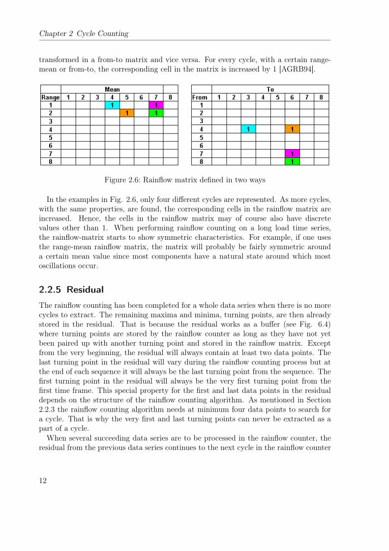
2.2.4 Rainflow Matrix
The rainflow-matrix is the result of the rainflow counting method. All extracted cyclesare stored in the rainflow-matrix. The matrix can be defined in several different ways,depending on how one wants to use the matrix. Fig. 2.6 shows two different rainflowmatrices that corresponds to the cycles extracted in the example of the non-recursiverainflow counter in Fig. 2.4 and 2.5. One possibility is to define the rainflow matrixas being from class x to class y, like the example matrix to the right in Fig. 2.6, i.e.,the cycle starts in class x and ends in class y. Another definition states that the axesof the matrix are equal to the range of the cycle (maximum - minimum) and its mean(| maximum + minimum | /2) shown as the second example in Fig. 2.6. Eitherway, the matrix contains the same information. A range-mean matrix can therefore be
9
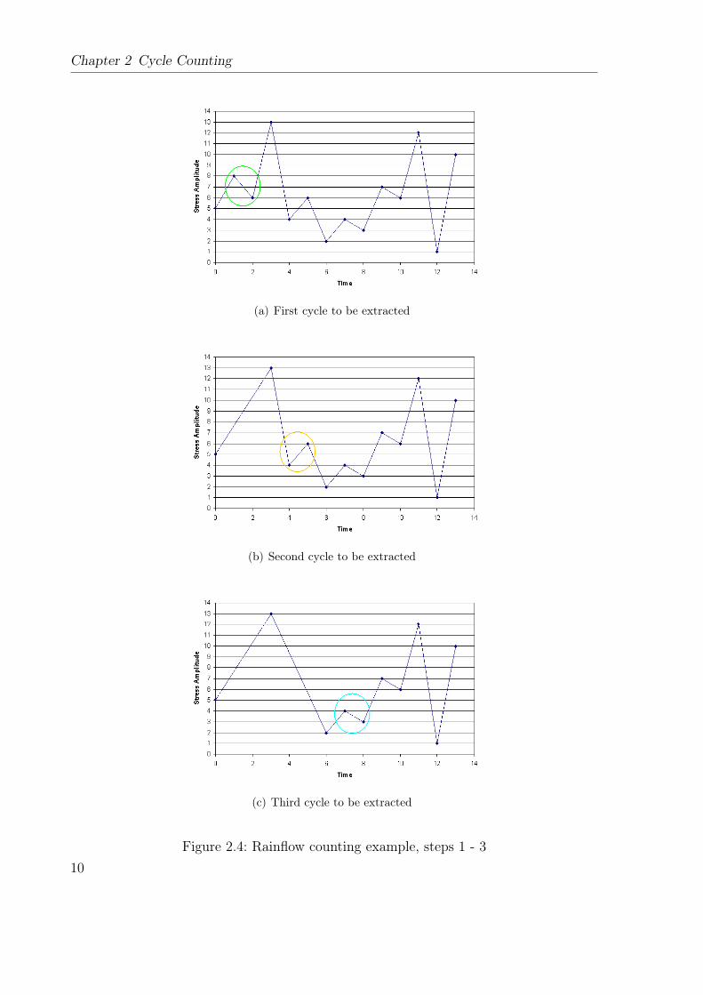
Chapter 2 Cycle Counting
(a) First cycle to be extracted
(b) Second cycle to be extracted
(c) Third cycle to be extracted
Figure 2.4: Rainflow counting example, steps 1 - 3
10

2.2 Rainflow Counting
(a) Fourth cycle to be extracted
(b) Fifth cycle to be extracted
(c) Resulting residual
Figure 2.5: Rainflow counting example, steps 4 - 6
11
Chapter 2 Cycle Counting
transformed in a from-to matrix and vice versa. For every cycle, with a certain range-mean or from-to, the corresponding cell in the matrix is increased by 1 [AGRB94].
Figure 2.6: Rainflow matrix defined in two ways
In the examples in Fig. 2.6, only four different cycles are represented. As more cycles,with the same properties, are found, the corresponding cells in the rainflow matrix areincreased. Hence, the cells in the rainflow matrix may of course also have discretevalues other than 1. When performing rainflow counting on a long load time series,the rainflow-matrix starts to show symmetric characteristics. For example, if one usesthe range-mean rainflow matrix, the matrix will probably be fairly symmetric arounda certain mean value since most components have a natural state around which mostoscillations occur.
2.2.5 Residual
The rainflow counting has been completed for a whole data series when there is no morecycles to extract. The remaining maxima and minima, turning points, are then alreadystored in the residual. That is because the residual works as a buffer (see Fig. 6.4)where turning points are stored by the rainflow counter as long as they have not yetbeen paired up with another turning point and stored in the rainflow matrix. Exceptfrom the very beginning, the residual will always contain at least two data points. Thelast turning point in the residual will vary during the rainflow counting process but atthe end of each sequence it will always be the last turning point from the sequence. Thefirst turning point in the residual will always be the very first turning point from thefirst time frame. This special property for the first and last data points in the residualdepends on the structure of the rainflow counting algorithm. As mentioned in Section2.2.3 the rainflow counting algorithm needs at minimum four data points to search fora cycle. That is why the very first and last turning points can never be extracted as apart of a cycle.
When several succeeding data series are to be processed in the rainflow counter, theresidual from the previous data series continues to the next cycle in the rainflow counter
12

2.2 Rainflow Counting
together with the new incoming data series. It can then be possible to form cycles fromdata points from different sequences, enabling detection of low-frequency load cyclesthat occur over a time frame limit.
Figure 2.7: Residual’s part in rainflow counting when several succeeding data series areto be taken into account
If an interruption in, or between, a time frame occurs, a special treatment of theresidual is required since the time series then contain a discontinuity. In this thesis, thehalf-cycles that are still present in the residual when an interruption occurs are countedas full cycles. This gives a conservative treatment of the load-sequence, i.e. a worst casescenario of the amount of damage that these loads could have caused.
To extract the half-cycles from the residual as complete cycles, the residual is simplyadded to itself and then processed by the normal rainflow counting algorithm, as seenin (2.1) [AGRB94]. Therefore, no changes have to be made to the rainflow algorithm inorder for it to process the residual, which is a big advantage of this procedure.
[residual] + [residual]rfc→ [residual] + {cycles} (2.1)
When joining the residual with a copy of itself, special care has to be taken if thenumber of elements in the residual is odd. In this case, the last element in the originalresidual or the first element in the copy have to be removed in order to avoid thosetwo maxima or minima ending up as neighboring elements. Such an occurrence wouldcorrupt the result of the rainflow counting algorithm. The rainflow algorithm only allowsan input sequence of alternating maxima and minima.
In Fig. 2.8, an illustrated example is given, describing how the residual is processed.Since this residual, which originates from the example in Fig. 2.5, has an even number
13

Chapter 2 Cycle Counting
(a) A copy of the residual is concatenated with the residualitself
(b) The half cycles from the residual and its copy have foundedfull cycles which can be extracted by the rainflow counting al-gorithm
Figure 2.8: Rainflow counting of the residual
of elements, no extra work has to be performed on the last element in the first residual.After concatenating this residual and its copy, the rainflow counter processes them. Inthis example, two cycles are extracted. Once again, the residual itself ends up as theremainder.
14
2.2 Rainflow Counting
2.2.6 Processing Succeeding Sequences
If rainflow counting is to be performed on a signal that consists of several succeeding load-sequences, the result formed by summation of the results from the individual sequencesdoes not, in general, correspond to the result generated when all sequences are consideredtogether at the same time [AGRB94]. A cycle could for example originate from anextremum in one sequence and another extremum from a second sequence. In order tohave the rainflow counting result for several individual sequences to comply with theglobal result, the following steps have to be added to the rainflow algorithm [AGRB94]:
1. Perform rainflow counting for each sequence and let the results be represented bythe tuple (cycles, residual)
2. Create a sequence by merging the residuals of each sequence, in the same order asthey occur in the global signal
3. Take the resulting sequence and split it up in cycles, according to the rainflowmethod
4. The global result of the rainflow counting is then reached by adding the extractedcycles from step 3 with the cycles from the individual sequences in step 1
The above steps are for rainflow counting that is performed offline. For online pro-cessing the sequences and residuals are not calculated separately. Instead, the residualfrom the rainflow counting for the previous sequence is concatenated with the presentsequence and then put into the rainflow counter, as in Fig. 2.7. When concatenating theresidual with the sequence, special care has to be taken to the last value in the residualand the first value in the sequence. Since it is not for certain that they are real turningpoints1 an extra evaluation has to be performed for these two data points. Here, it isdetermined if these two data points are turning points or not. If they are not turningpoints they are removed from the sequences.
2.2.7 Preprocessing Functions
Classification
As seen in Fig. 2.1 and 2.2, the load-axis has been divided into classes. This discretiza-tion is done to suppress noise, reduce execution complexity and to give the rainflowmatrix a more uniform appearance, independent of which sensors that are used. Theclassification is performed by calculating the range between the global maximum andminimum value in the time series, splitting this range in classes and then giving eachdata point a class-number instead of its real value. The number of classes used dependson the desired resolution, the available calculation performance and/or the amount of
1 See the Maxima and Minima Filter in Section 2.2.7
15

Chapter 2 Cycle Counting
available memory. If a larger number of classes can be used, a higher accuracy can beachieved. In the work presented here, 164 classes were used since this has shown to begood practice by the tests performed by GE Energy. The limitation of the number ofclasses was due to finite memory size on the PLC2 where the program was executed.The rainflow matrix is very memory demanding since the memory on the PLC couldonly be statically allocated and every cell in the matrix has to be able to store an integervalue that ranges up to about 108, assuming the worst case number of cycles. If the PLCwould have had dynamic memory it would have been possible to change the declaredvariable size during execution, making the memory handling much more efficient andflexible.
Since the rainflow counter implemented in this thesis is to be used online, the definitivemaximum and minimum value from the time series are not known in advance3. This isa considerable challenge since the maximum and minimum have to be known in orderto make an optimized layout of the classes. To solve this, one can use experimentallyfound extremum values instead of the real maximum and minimum. These extremumvalues can be achieved by letting the wind-turbine run in normal mode and then force anemergency stop. An emergency stop exposes the wind turbine to extreme loads. It is notlikely that the wind turbine will suffer from larger loads than those during emergencystop. A disadvantage of this method would be that the classes are spread over a value-space probably much larger than needed, since such extreme loads are very rare. Thisresults in a bad resolution and makes the method less accurate. Another approach wouldbe to ignore the extreme loads, or at least to classify them in the highest class possible,in order to increase the accuracy for the smaller and more frequent loads. However,according to [Joha99] the largest loads, even though the number of them is marginal,constitute a majority of the total damage and therefore these loads can not be neglected.
The chosen solution was to use two rainflow matrices instead of one. One of theserainflow matrices was defined to be used for a limited value-space, offering a high resolu-tion in this area. All normal loads will be represented in this matrix. Every cell in thismatrix is defined to be able to store an integer value with 32 bit resolution. Also thenumber of the most common cycles should therefore fit in this matrix, considering anoperational lifetime of the system of 20 years. For derivation of the worst case numberof cycles see Section 3.2. Extreme loads that do not fit in the value-space covered by thehigh resolution rainflow matrix are stored in the low resolution rainflow matrix. Thismatrix covers a very large value-space, however it has a low resolution since it also usesthe same number of classes as the first matrix. The loss of accuracy in the low resolutionmatrix is of less importance since there are only a handful of cycles that will be storedthere. Therefore, it is only of significance to store the approximate range and meanof these load cycles. Each cell in the low resolution matrix is only defined to store an
2 PLC: Programmable Logic Controller3 For an offline rainflow-counter the definitive maximum and minimum value from the time series are
known
16

2.2 Rainflow Counting
Figure 2.9: Description of a high and low resolution rainflow matrix
integer value with 16 bit resolution, which is expected to be more than enough. Thelow resolution matrix covers a value space ten times as large as the one covered by thehigh resolution matrix. For simplicity reasons, the low resolution matrix also covers thevalue-space of the high resolution matrix, even though this part of the matrix will alwaysbe empty since it is already represented. The real value-space that the low resolutionmatrix covers is for the mean-axis symmetrically located around the high resolution ma-trix and for the range-axis it starts right after the end of the high resolution matrix’svalue-space. The proportions between the high- and low-resolution rainflow matrices canbe seen in Fig. 2.9. If the high resolution would be used over the entire value-space itwould result in a data amount of about 11MB per rainflow matrix. With the suggestedsolution presented here, only 160KB of memory is needed, i.e. about 1.5% of 11MB. Forevery monitored sensor, the monitoring system needs a separate rainflow matrix. Thismeans that the amount of needed memory for the rainflow matrices would increase fastwhen the number of monitored sensors increase. Therefore, it was important to keepthe representation of the rainflow matrix as memory efficient as possible.
When performing classifications, every turning point is discretized to one of the classesu1 < u2 < ... < un. That means that the turning points can only be associated with ndifferent values. Two ways of performing the classification are presented here: [Johb99].
1. Each turning point is classified to the closest class, i.e.
17

Chapter 2 Cycle Counting
xdk = ui if ui −
ui − ui−1
2≤ xk < ui +
ui+1 − ui
2(2.2)
(where u0 = −∞ and un+1 = ∞, i.e. the outermost borders of the first and thelast class are open). The classification may cause successive values to take thesame discrete class. This is dealt with by the maxima and minima filter.
2. A minimum is classified to the nearest lower value from the classes u1 < ... < un−1
and a maximum to the nearest higher value from the classes u2 < ... < un.
The advantage with the first method is that the classification errors are smaller thanin the second method. This leads to smaller errors when calculating the damage. Thesecond method, on the other hand, gives a conservative classification but with less ac-curacy. The reason why the second method is conservative is that it always represents aturning point that lies between two class levels as the largest one when the turning pointis a maximum and as the smallest one when the turning point is a minimum [Johb99].The damage calculations then gives a larger or equal damage result compared to if thefirst classification method is used. From a safety aspect, it is of course essential that thelife meter always shows at least as much damage as the component has actually sufferedand it must for no cases show less. For theses reasons, the second method was chosento be used throughout this work.
Within a class, all noise will be suppressed because every value within the class getsclassified as the same class. Noise occurring on a limit between two classes would onthe other hand cause oscillations between those classes. In order to suppress this noise,a reset level, also called hysteresis, is introduced. With the reset level, the rainflowalgorithm will only count a cycle if it is larger than the reset level. In this thesis thereset level was set to the size of one class, i.e. only cycles with a range larger than oneclass are counted. The reset level has been chosen to one class since practical experiencehas shown that this gives good noise filtering without loss of important information.
Maxima and Minima Filter
As mentioned in Section 2.2.3, the rainflow counting algorithm takes only the extremumvalues of the entire load sequence as an input. Therefore these have to be extractedfrom the rest of the data points. This is done by the max/min filter. This filter onlyextracts all real extremum values, i.e. no saddle-points are considered.
The first data point, in the series of turning points, will not be a turning point, but thefirst data point from the first input sequence. This is because it can not be determinedif the first data point is a maximum or minimum since there are no previous values tocompare it with. Therefore, the very first and last data point from the sequences willalways be included to the series of turning points in order to be on the safe side, i.e. inorder not to have any turning points neglected.
18

2.3 Conclusions
2.3 Conclusions
The rainflow counting method was chosen for extraction of load cycles from the loadsequences. Best practice has shown to use the rainflow counting method when acquiringrelevant information from a load sequence in order to monitor the lifetime of a compo-nent. The rainflow counting method can also be used for online processing, which was arequirement for this thesis. A non-recursive version of the rainflow counting algorithmwas selected for implementation.
In case of a discontinuity in an incoming time frame, the residual has to be processed,by the rainflow counter, and be reset in order to keep the overall result valid. With thisfeature implemented, the system becomes very robust to handle outer disturbances tothe sensors and/or the data acquisition system.
The classification of the data points in the time frames were performed in a conser-vative manner. The conservative classification method was chosen before the least-errormethod in order to ensure that the damage calculated is always larger than in reality.
To make online rainflow counting possible, a new approach had to be found for thelayout of the classes. By having two rainflow matrices, one with high resolution fora small value-space and one with low resolution for a large value-space, all necessaryinformation from the rainflow counting could be stored. This was also a very memoryefficient solution, demanding only a fraction of the memory needed for other possiblesolutions.
19

Chapter 2 Cycle Counting
20

Chapter 3
Fatigue Analysis
3.1 General
Fatigue, the loss of strength and other important mechanical properties as a result ofcyclic loading over a period of time, is a general phenomenon occurring in most materials[DeJi03]. Usually, components are not destroyed by a single large load, but by theaccumulation of many smaller loads [DrHa95].
Generally, fatigue is seen as a rate independent process [Johb99]. This means that thetime interval between two loads is of no interest for fatigue, only the dimensions of theloads effects the lifetime. Therefore, the maximum and minimum values of the loads arethe most important parameters to study.
In order to illustrate the fatigue properties of a material, a SN-curve (also called aWöhler curve) is often used. A SN-curve shows the relationship between stress amplitudeand cycles to failure. The SN-curve, see example in Fig. 3.1, is defined as:
N(Si) =
{
αS−mi , Si > S∞
∞, Si ≤ S∞
(3.1)
where N is the number of cycles to failure and Si is the stress corresponding to load i.α and m are material parameters where α describes the fatigue strength of the materialand m is the damage exponent. The higher the stress amplitude, the less number ofcycles to failure. For some materials, below a certain stress amplitude, S∞, the numberof cycles to failure approaches infinity. This is called the endurance limit of the materialand is a material property. As can be seen in the example in Fig. 3.1, it is state-of-the-art to present the SN-Curve with the load range on the y-axis and the number ofapplied load cycles on the x-axis.
In Table 3.1, the damage exponent m for different materials is presented. For somematerials, after a specific cycle limit another damage exponent with a larger value shouldbe used. This makes the SN-curve for higher number of cycles more horizontal. Hence,even load cycles of a small amplitude will still have some impact, even though it isdiminutive, on the lifetime of the component since the number of cycles applied withthis amplitude is enormous.
21

Chapter 3 Fatigue Analysis
Figure 3.1: Example of a SN-curve
Material Used for m-I m-II Inflection point (nbr of cycles)
Epoxy resin Blades 10 NA NACrude steel Tower 3 5 5 · 106
Steel Main-shaft 4.9 7.3 7.7 · 105
Table 3.1: Damage exponent m-I and -II for different materials
Since the design lifetime for a wind turbine is mostly 20 years it has to endure about108 cyclic loads during this time, assuming a 1 Hz oscillation [DeJi03]. This calls fora very robust construction and design of wind turbines, making the study of fatigueprocesses highly important1.
3.2 Damage Calculation
Fatigue damage d is defined as the number of applied load cycles n (in this case countedwith the rainflow counting method), of a certain amplitude, to the number of cycles tofailure N.
1 Wind turbine components are generally overdimensioned in order to ensure security. A more preciseanalysis of the actual fatigue on the different components would enable a better and more economicaldimensioning of them, thus reducing material costs.
22

3.2 Damage Calculation
d =n
N(3.2)
Given that a component is usually exposed to cycles of different amplitudes, thetotal damage can be defined by Palmgren-Miner’s rule [Mine45, Palm24], which can befound in (3.3). Palmgren-Miner’s rule summarizes the damage from each cycle for alldifferent amplitudes. The accumulated damage is represented by D, and i is the discretenumbering of all different load amplitudes. The accumulated damage is less then orequal to the value 1. When D is larger than 1 the component has exceeded its expectedlifetime and is, at least theoretically, broken.
D =∑ ni
Ni
≤ 1 (3.3)
Experiments have shown that components can fail, in reality, for D-values as low as0.2 [Echt96]. This means that Palmgren-Miner’s rule has to be used with caution, e.g.by multiplying it with a safety-factor in order to keep the fatigue-damage under thecritical limit. Recent research, see [JoSM05], shows that Palmgren-Miner’s rule can bemade conservative and secure if the SN-curve, from which the values for Ni are derived,is estimated using variable amplitudes instead of constant amplitudes. Estimating theSN-curve with constant amplitudes means that only one load amplitude is tested at atime. The result is the amount of load-cycles, with a certain load amplitude, that thecomponent can survive before it fails. With variable load amplitudes, certain referenceload spectrums are used instead of constant load amplitudes. The values in this the-sis, that are derived from SN-curves, all come from SN-curves estimated with constantamplitudes.
A comfortable way of defining fatigue damage uses Damage Equivalent Load (DEL)Seq and its corresponding reference number of load ranges, neq. The new definition ofdamage is then as follows [JoSM05]
D =∑ ni
Ni
=∑ ni
αS−mi
=1
α
∑
niSmi =
neqSmeq
α(3.4)
where
Seq =(
∑
viSmi
)1/m
=
(∑
niSmi
neq
)1/m
(3.5)
vi is the relative frequency of occurrence of the load amplitude and neq is the reference-number of cycles in the time frame. When the cycle-counting result is scaled up to atime-frame of 20 years, neq is mostly chosen to be 4.74 ·108. This reference number is thenumber of oscillations resulting when one takes a 1 Hz oscillation, assuming oscillationsfor 20 years and taking into account an inactivity of 25 %. The inactivity comes fromthe turbine’s cut-in and cut-out behaviour, i.e., a turbine operates if the wind speed isabove the cut-in level and stops if the wind speed exceeds the cut-out level. A challenge
23

Chapter 3 Fatigue Analysis
with (3.5) is that it can not be determined if m-I or m-II is to be used for the outerexponent 1/m since it does not relate to a certain number of cycles, in opposite to theinner exponent that always relates to a certain ni. The solution chosen was to keepthe procedure conservative by using m-I as the outer exponent because this gives largervalues for the Seq.
Component Position at Component Mechanical Load m Seq_max (kNm)
Blade 2.75m from hub center Bending, edgewise 10 1089.6Blade 2.75m from hub center Bending, flapwise 10 979.0
Main shaft Main-shaft flange Torsion 4 110.7Main shaft Main-shaft flange Torsion 6 192.3Main shaft 0.1m from flange bending 90◦ 4 4197.4Main shaft 0.1m from flange bending 90◦ 6 5212.4
Tower 91.77m height Torsion 4 562.7Tower 6.01m height bending 0◦ − 180◦ 4 3357.6Tower 6.01m height bending 90◦ − 270◦ 4 4199.6
Table 3.2: Designed maximum DEL for different components and m exponents[GEWE05]
Since the designed maximal damage equivalent load, Seq_max, was given for the windturbine components used for the tests in the presented work, it was desirable to useanother approach to represent the fatigue-damage. In equation 3.6, damage D is definedas the relationship between Seq and Seq_max, i.e., measured DEL against a designedmaximum DEL. It is trivial that D, also in this definition, will be less then or equal to1 if the component is not broken.
D =Seq
Seq_max
≤ 1 (3.6)
When comparing Table 3.1 and Table 3.2, it can be observed that the damage-exponents m, for the main-shaft and tower, are not the same. The reason for this is thatGE Energy, who has provided the information for these two tables, only calculates themaximum DEL for different components, positions, and for certain damage-exponents,mostly only for even integer numbers. Since this was the case, the closest lower eveninteger damage-exponent was chosen for the calculations because it gives a conservativeresult when calculating the DEL’s.
3.3 Conclusions
• The fatigue properties of a component can be illustrated in a SN-curve
24

3.3 Conclusions
• With the help of the Palmgren-Miner’s rule, the accumulated damage to a com-ponent can be calculated if the number of cycles to failure, for every possible loadamplitude, is known.
• The Palmgren-Miner’s rule has to be used with caution, for example multiplyingit with safety-factors, because components can break for damage values as low as0.2 instead of the theorethical 1.0
• A comfortable way of representing fatigue-damage is by using DEL
• The total damage to a component is calculated as the measured DEL against thedesigned maximum DEL
25

Chapter 3 Fatigue Analysis
26

Chapter 4
Wind Turbine Setup
4.1 Structure
The structure of a GE 1.5 s/sl wind turbine hub and nacelle is presented in Fig. 4.1.This was the target wind turbine model for the installation of the prototype monitoringsystem. The components regarded in this thesis were blades, main-shaft, and tower.
Figure 4.1: Model of a GE 1.5s/sl wind turbine [GEWE04]
Controlled parts in the wind turbine are the pitch angle of the blades, engine speedand yaw angle of the top-box. The pitch angle of the blades determines the attack angle
27
Chapter 4 Wind Turbine Setup
of the blades toward the wind. 0◦ pitch angle means that the maximal area of the bladesis turned against the wind direction. If the wind gets to strong, the turbine increases thepitch angle in order to decrease the attack area of the blades. By doing this, the turbinecan operate in higher wind speeds without exceeding the security limits by overloading.The purpose of the yaw angle of the top-box is to keep the top-box positioned towardthe wind direction. In case of storm, the yaw angle is changed and the top-box is turnedout of the wind direction in order to avoid overloading and possible damages.
4.2 Sensors
Throughout this work, the sensors in Table 4.1 were used. These sensors were availablein both the simulation environment and in the real turbine.
Component Value Sensor Abbreviation
blade bending moment edgewise blxMeblade bending moment flapwise blxMf
main-shaft torsion mshTmain-shaft bending 90◦ mshM90
tower torsion toTtower bending 0◦ − 180◦ toM0tower bending 90◦ − 270◦ toM90
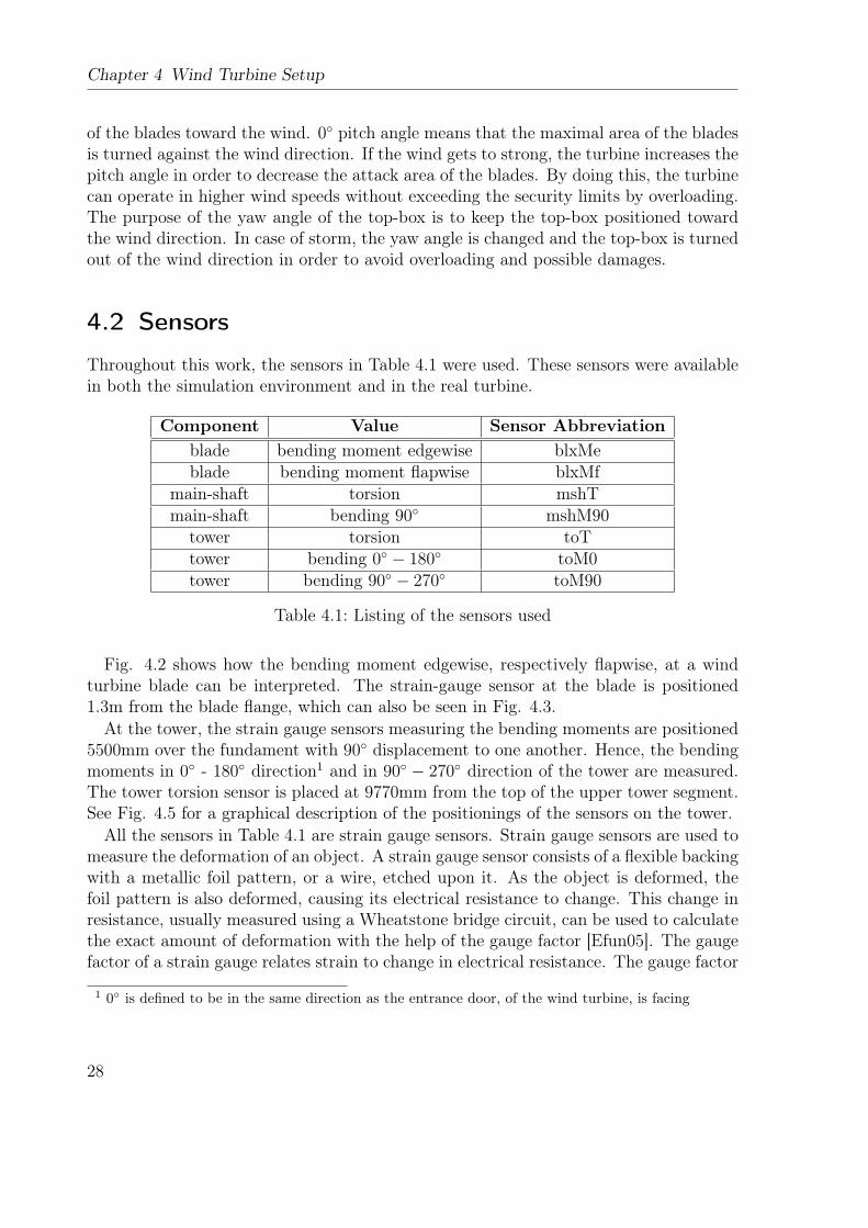
Table 4.1: Listing of the sensors used
Fig. 4.2 shows how the bending moment edgewise, respectively flapwise, at a windturbine blade can be interpreted. The strain-gauge sensor at the blade is positioned1.3m from the blade flange, which can also be seen in Fig. 4.3.
At the tower, the strain gauge sensors measuring the bending moments are positioned5500mm over the fundament with 90◦ displacement to one another. Hence, the bendingmoments in 0◦ - 180◦ direction1 and in 90◦ − 270◦ direction of the tower are measured.The tower torsion sensor is placed at 9770mm from the top of the upper tower segment.See Fig. 4.5 for a graphical description of the positionings of the sensors on the tower.
All the sensors in Table 4.1 are strain gauge sensors. Strain gauge sensors are used tomeasure the deformation of an object. A strain gauge sensor consists of a flexible backingwith a metallic foil pattern, or a wire, etched upon it. As the object is deformed, thefoil pattern is also deformed, causing its electrical resistance to change. This change inresistance, usually measured using a Wheatstone bridge circuit, can be used to calculatethe exact amount of deformation with the help of the gauge factor [Efun05]. The gaugefactor of a strain gauge relates strain to change in electrical resistance. The gauge factor
10◦ is defined to be in the same direction as the entrance door, of the wind turbine, is facing
28

4.2 Sensors
Figure 4.2: Cross section of a wind turbine blade describing how the pitch-angle, theflap direction, and the edge direction should be interpreted
GF is defined by the following equation:
GF =△R/RG
ǫ(4.1)
where RG is the resistance of the undeformed gauge, △R is the change in resistancecaused by strain, and ǫ is the strain. The gauge factor is usually provided by themanufacturer of the strain gauge.
The strain gauges on the turbine blades are calibrated by halting the turbine andputting each blade, one after another, in the vertical position. By knowing the weightof the blade and the exact position of the strain gauge on the blade, the strain gaugecan then be calibrated since the load moment occurring at the actual position is known.The calibration is performed manually and only at low wind speeds.
29
Chapter 4 Wind Turbine Setup
Figure 4.3: Description of the positioning of the strain gauge sensor on the blade [Feic05]
Figure 4.4: Description of the positioning of the strain gauge sensors on the main-shaft[Feic05]
30

4.2 Sensors
Figure 4.5: Description of the positioning of the strain gauge sensors on the tower
31

Chapter 4 Wind Turbine Setup
32

Chapter 5
Hardware Setup
5.1 Hardware In The Loop
For the development of the embedded software, a HITL1 real-time simulation system, seeFig. 5.1, was used. A HITL system simulates a real system, in this case a wind turbine.The complete behavior of a wind turbine, from a controller-unit’s point of view, wasrepresented here. There was no difference for the wind turbine controller running on theHITL and running on a real turbine. It was not necessary to perform any changes tothe controller when changing between these two working environments.
Figure 5.1: Block diagram of an embedded system connected to a HITL-simulator
The HITL simulator was built upon COTS2 hardware, a real-time operating system(QNX) and a real-time simulation platform (RT-LAB) working with the Matlab toolboxSimulink. See Fig. 5.2 for the entire setup structure. The system consists of a RT-LAB command station, which is often called host PC, a QNX target, a workstation
1 HITL: Hardware In The Loop2 COTS: Commercial-Off-The-Shelf
33

Chapter 5 Hardware Setup
for SCADA3, an interface PLC, the tested PLC and various cables for LAN4, CAN5,RS4226, and digital and analog I/O’s7. The QNX-system runs on an industrial PC8.All actual computations and communications takes place in this system. By using theQNX real-time operating system, the real-time performance is ensured. VisuPro is aSCADA system that is monitoring and controlling the Bachmann controller via a LAN.With VisuPro, one can change the parameters of the PLC, start/stop the wind turbine,regulate the pitch angle manually, monitoring the main parameters such as rotor speed,wind speed, pitch angle, voltage etc. VisuPro is used for both simulation purposes andfor management of real GE wind turbines. [GEGR04].
Figure 5.2: HITL system architecture [GEGR04]
Development of the software can be performed with the HITL prior to actual field-testing. This is a large advantage because it would be very expensive and precarious todevelop and test new software directly on a real wind turbine. It would be precarioussince errors always occur in the first few revisions of new software. When testing thesoftware on the HITL, it does not matter if an error appears because the HITL caneasily be stopped and restarted without any damage taking place. If the same errorwould have occurred on a real wind turbine it could, if it was a serious error, put
3 SCADA: Supervisory Control And Data Acquisition4 LAN: Local Area Network5 CAN: Controller Area Network6 RS422 is a serial data communication protocol7 I/O: Input/Output8 An industrial PC is very similar to a normal PC, but more robust and stable. It is eg. more resistant
to a harsh environment.
34

5.2 Development Setup
out a security system and push the turbine into an insecure state. Furthermore, moremeaningful tests can be performed with a HITL than with a real system. With a HITLone can easily control all different kinds of input, which would not be the case for atrue system, thus making it possible to build up an arsenal of different test cases. Thesecan contain extreme conditions, which can be very hard to test in reality because theyare too rare and/or too hazardous. The test cases can easily be run through the HITLsimulator in order to determine if the developed program operates as expected.
5.2 Development Setup
Execution of the monitoring system was carried out on a Bachmann M1 ControllerSystem. The Bachmann M1 is a modular PLC consisting of one CPU module that canbe connected with several analogue or digital I/O modules.
The controller in the development setup, see Fig. 5.3, was an exact copy of the con-troller that is present in the wind turbine GE 1.5 s/sl from GE Energy. This improved theprospects of success for the later installation in a turbine of the same type. The HITL-system substitutes all real I/O-signals that are normally connected to the controller withsimulated I/O-signals. Inputs to the controller are all sensor values. Outputs are thecontrol signals, to all the controlled components in the wind turbine, calculated by thecontroller. Controlled components in the wind turbine are, as described in Section 4.1,the pitch angle of the blades, the engine speed, and the yaw angle of the top-box. TheHITL-system receives the output signals from the controller and includes them in thecalculations of the new input signals.
The lifetime monitoring program runs on the LUM module CPU (as seen in Fig. 5.3).
5.3 Prototype Setup
The ambition of the hardware setup was that the new monitoring system should beadded to the wind turbine without any changes to the present system. This would beadvantageous since the monitoring system could then be added to already existing tur-bines at rather low costs. Furthermore, performing changes to an existing wind turbinemodel would force the producer of the turbine to once again carry out security certifi-cation of the model. This would also result in large costs. Therefore, all componentsfrom the LUM-project were formed as true add-on modules, thus avoiding the necessityof changing the present system setup.
The already existing communication between the hub and the nacelle was carried outover a slip ring that was located around the main-shaft. As can be seen in Fig. 5.4, theLUM-module in the hub was connected to the nacelle module via CAN over WLAN9
9 WLAN: Wireless Local Area Networ
35

Chapter 5 Hardware Setup
Figure 5.3: System overview of the development setup [Feic05]
with a base frequency of 2.4 GHz (IEEE 802.11 b/g). The reason for using WLAN wasthat all communication slots at the slip ring, on the target turbine for the prototypeinstallation, were already full. Using WLAN in a wind turbine had only been tested oncebefore by GE Energy10, although never for a permanent field bus connection. There weredoubts regarding installing a WLAN in the hub and nacelle of a wind turbine since thehub has thick cast steel walls that could shield or attenuate the signal. Another reasonfor the doubts were that there are very strong electromagnetic fields from the generatorin the nacelle, that could disturb the signal. However, since the wavelengths for a WLANwith 2.4 GHz base frequency are
λ =c
f(5.1)
λb/g =300 · 106m/s
2.4GHz≈ 13cm (5.2)
10 GE Energy has performed a field test with WLAN in a wind turbine. The test was carried out in2004 in Magdeburg, Germany, in the wind park Wellen II.
36
5.3 Prototype Setup
the thickness of the material between the two WLAN access points may not exceed13cm in order not to disturb, or even block, the communication. Using WLAN wasfound to be a feasible approach worth testing because there are several places at the hubwhere the thickness is less than 13cm [Feic05]. In practical tests, during the prototypeinstallation, it turned out that the WLAN communication works very well, despite theharsh environment.
Figure 5.4: System overview of the prototype setup [Feic05]
The LUM nacelle module was connected via a fiber optic cable, installed exclusivelyfor the LUM system, down to the LUM main station11. It did not use the alreadyexisting fiber optic communication line in order to ensure that the communication fromthe monitoring system does not disturb the ordinary communication between the topbox and the main controller.
The LUM main station was connected to the main controller via an Ethernet networkin order to enable the monitoring system to access some data from the main controller.As an extension, this connection is also meant to be used the other way around, i.e.that the main controller can access data from the LUM system in order to be used tooptimize the lifetime of the wind turbine.
11 The LUM main station was installed at the second platform in the wind turbine, about 10 m abovethe turbine foundation
37

Chapter 5 Hardware Setup
5.4 Conclusions
Simulations were performed with a HITL real-time simulation system. With the HITLsystem, all necessary inputs for the wind turbine controller could be simulated. Thechosen wind turbine controller was an exact copy of the one present in the GE 1.5 s/slturbine. The entire software development was carried out with the help of this controllerand the HITL simulator.
The monitoring system was constructed completely as an add-on in order to avoidcarrying out any changes to the existing setup of the wind turbine. This makes thesystem more cost efficient and easy to install.
The communication between the modules in the nacelle and the hub, in the prototypesystem, were provided by a CAN over WLAN connection. This was a new approachthat had only been tested once before by GE Energy. However, tests showed that thecommunication was stable and reliable.
A new fiber optic cable between the nacelle and the main cabinet was also includedin the prototype setup. Since the monitoring system only uses its own physical com-munication connections it could be ensured that the system would not disturb anycommunication from the current wind turbine controller.
38

Chapter 6
Developed Software
6.1 Development Environment
The monitoring system was implemented with the Bachmann M-PLC 3 developmentenvironment. This enables the programmer an easy usage of the IEC-61131-3 program-ming languages. The system was implemented using structured text (ST), which is oneof the five programming languages defined in the IEC standard for PLC-programming.The other four are instruction list (IL), ladder diagram (LD), function block diagram(FBD), and sequential function chart (SFC).
6.2 Program Organization Units
In M-PLC 3, a Program Organization Unit (POU) can be a function, a function block,or a program.
Functions normally have multiple input and only one output. Functions can only callother functions, no function blocks or programs can be called. There is no own memoryreserved for functions.
Function blocks are much like functions but they can have no, or multiple, outputs andcan even have combined inputs/outputs. Each function block has its own memory andtherefore they have to be instanced. Having its own memory means that a function blockkeeps the values of its variables, after being processed, for the next process call. Thus,two calls to a function block, with the same input parameters, can generate differentoutput values. Function blocks can call functions and other function blocks. Although,they can not call programs.
Programs are the main program organization unit. They can be globally accessedthroughout the whole software project. Therefore, they can not be instanced. Pro-grams can be called with or without parameters. Programs can only be called by otherprograms. As well as for a function block, a program also have its own memory.
39

Chapter 6 Developed Software
6.3 Design
During this thesis, several design proposals were developed and taken under consider-ation. Two of the designs were implemented. These two designs are both described inthe following two sections.
6.3.1 First Design Approach
As can be seen in Fig. 6.1, the system takes data series as input. The data seriescan be retrieved from an arbitrary sensor on the wind turbine that measures force ormoment. This thesis concentrates on the sensors measuring tower moment and torsion,main shaft moment and torsion, and blade deflection in edgewise and flapwise direction.These components are the most central in the wind turbine construction. The sensorsjust mentioned were all given on both the HITL-system and on the real wind turbinethat was used for testing. Thus, appropriate comparison between simulations and realmeasurements were possible.
Figure 6.1: Software flowchart for the first design approach
The incoming data series were retrieved from the sensors, with the help of a dataacquisition system1, during a time-frame of 10 minutes. Approximately 27 Hz samplingfrequency was used, enabling detection of oscillations up till about 13.5 Hz. Thus, eachdata series contain 16.384 data samples. The input data series first enters a maximaand minima filter function block. The turning points that are extracted here continuesto the classification function block. Here, incoming data gets classified according tothe norms for conservative classification presented in Section 2.2.7. The now classifiedturning points follow to a new maxima and minima filter function block that filter outany succeeding turning points that may have been discretized to the same level by theclassification function block. This is necessary in order to preserve that only true maximaand minima data points enters the rainflow counter. The data points that are filtered outin the last filter are considered to be noise, since they are part of cycles occurring withinthe limits of one class. The reason, why a maxima and minima filter has to be performed
1 See [Feic05] for more information on the data acquisition system
40

6.3 Design
twice, instead of once after the classification, is that the classification function needs toknow if the current turning point is a maximum or a minimum to be able to carry out aconservative classification of it. From the second maxima and minima filter the turningpoints are sent onward to the rainflow counter. The rainflow counter takes the maximaand minima and combine them into cycles, which are then stored in the rainflow matrix.The fatigue calculation block takes the rainflow matrix as input and uses it to calculatethe fatigue. At the end of each processing cycle, the estimated remaining lifetime isdisplayed in the form of a so called life meter. After this, a whole cycle of the program,for one sensor, has finished. The program returns to its starting state and proceeds withthe same process for any other sensor that is to be monitored. If all sensors have beenprocessed, the program goes to its idle state and waits for the next time frame to arrive.
The transfer of large data-blocks, e.g. rainflow matrices and time frames, between thedifferent function blocks gives a high processor load. To avoid this, pointers were usedat all places in the system where data-blocks of significant size were needed as inputparameters.
6.3.2 Second Design Approach
The second design approach was basically the same as the first one, but with one majordifference, namely the classification. In opposite to the first design approach, the classifi-cation was included in the rainflow counter function block in the second design approach.Hence, the second maxima and minima filter became unnecessary. The reason why theclassification was performed before the rainflow counting in the first approach was thatin that way more data points were filtered out before reaching the rainflow counter. Thiswould then lead to less execution complexity. However, by doing the classification be-fore the rainflow counter the result becomes less accurate because the rainflow countingmethod is carried out with classified values. Since the result from the classification is inany case conservative this would not be a security issue. Although, the lifetime of themonitored components would be decreased slightly faster than in reality. The implica-tion of this would be increased costs. It was also found that in the already availableoffline rainflow counter included in the commercial signal processing tool FAMOS, usedby GE Energy, the classification was performed internally by the rainflow counter. Thisfurther encouraged the use of the second design approach since this made it possibleto validate the developed system by comparing with results achieved from GE Energy’scalculations.
41

Chapter 6 Developed Software
Figure 6.2: Software flowchart for the second design approach
6.4 Developed POU’s
6.4.1 Program Lifetime_calc_main
The program lifetime_calc_main is the main program of the developed monitoringsystem. This is called for every incoming time frame from every sensor. The calls comefrom the main program of the data acquisition system.
In the lifetime_calc_main program there is a setting that enables the user to chooseto use the implementation with the external or internal classification when performingthe calculations. By setting the boolean variable rfc_internal_classification to TRUE orFALSE, the user can decide which approach to use. Default value of rfc_internal_classificationis TRUE.
From the lifetime_calc_main program, all calls are made to the different functionblocks used in the monitoring system. The lifetime_calc_main program is arranged insuch a way that after every finished call to a function block it returns to the callingprogram. The reason for this is to keep execution cycles short, preventing violation ofthe real-time properties of the system. This means that before a time frame has beencompletely processed, several calls to the lifetime_calc_main program has to be made.First when the lifetime_calc_main program’s output is set to true is the processing ofa time frame completed.
The first task for the main program, for every new incoming time frame, is to controlthe integrity of the time frame. This is done by checking the time that the time framecontain. The time contained have to be exactly the same as expected, with millisecondaccuracy, in order to be accepted. In this system, every time frame is supposed to be 10minutes long, thus it should contain 600 000 ms. The time frame data structure has alsoan error flag that can indicate several kinds of errors. This flag is also controlled beforeletting the time frame pass to the calculation function blocks. In case of a corrupt timeframe, the time frame is thrown away and the residual for the corresponding sensor isprocessed by the rainflow counter, and reset, and the program goes back to its idle statewaiting for the next time frame/call.
42
6.4 Developed POU’s
6.4.2 Function Block Filter_max_min_REAL
The function block filter_max_min_REAL was used in the first implementation ap-proach. In this implementation version, it was the first of two maxima and minima filterfunction blocks. It takes a time series of floating point values as input and filters it.The outputs from this function block are the number of turning points that the timeseries contained and an array with the turning points themselves. Here, a turning pointmeans an extremum, maximum or minimum. All possible saddle points are also filteredout by this function block. If several succeeding data points in the time series have thesame value and they together constitute an extremum, only one of them is kept. Thus,the output array with turning points only contain alternating maxima and minima. Fig.6.3 shows the flowchart of the function block filter_max_min_REAL.
Figure 6.3: Flowchart for the maxima and minima filter algorithm
43

Chapter 6 Developed Software
6.4.3 Function Block Filter_max_min_INT
The function block filter_max_min_INT was only used for the first implementationapproach. It was used as the second maxima and minima filter function block. Thisfunction block is very similar to the function block filter_max_min_REAL. Although,it takes an array of integer values as input instead of floating point values. It alsocontrols if the last value in the residual, i.e. the last value from the previous time frame,is really a maximum or minimum by comparing with the first data point in the presenttime frame. This verification has to be carried out for every time frame, because the lastdata point from each time frame is automatically included to the residual, to ensure thatno possible maximum or minimum are lost. Except for controlling the last data pointin the residual, the main functionality of the function block filter_max_min_INT wasto remove possible succeeding data points with the same value that could have arisenduring the external classification process, present in the first implementation approach.
6.4.4 Function Block Filter_max_min_REAL_v2
By using the function block filter_max_min_REAL_v2, the functionality of the func-tion block filter_max_min_REAL and filter_max_min_INT are combined. It wasconstructed to filter a time frame of floating point values regarding its turning points,as in filter_max_min_REAL, and also for controlling the last value in the residual,as in filter_max_min_INT. The function block filter_max_min_REAL_v2 was onlyused in the second system implementation, with the classification performed internallyin the rfc_v2 function block. Since the classification is performed internally, the filterfunctionality does not have to be splitted into two function blocks2.
6.4.5 Function Block Rfc
The most central function block in this thesis was the rfc. The rfc function block performsrainflow counting on the incoming turning points according to the non-recursive rainflowalgorithm presented in Section 2.2.3. The most important outputs from the rfc are thetwo rainflow matrices, the high resolution rainflow matrix and the low resolution rainflowmatrix, and the residual.
6.4.6 Function Block Rfc_v2
An extended version to the function block rfc is the rfc_v2. The difference betweenrfc and rfc_v2 is that rfc_v2 has the classification functionality integrated in its ownfunction block, according to the second design approach. This makes the results comingfrom rfc_v2 more accurate than the ones from rfc. Except this, there is no differencebetween rfc and rfc_v2.
2 Compare with Fig. 6.1 and Fig. 6.2
44

6.4 Developed POU’s
Figure 6.4: Flowchart for the rainflow algorithm
45

Chapter 6 Developed Software
6.4.7 Function Block Damage_calc
With the two rainflow matrices, calculated by rfc or rfc_v2, as inputs, the damage_calcfunction block calculates the damage that the respective component has suffered from,or to be more exact, the DEL3. Other inputs needed for this calculation are the materialparameters and designed maximum DEL for the component that the actual time seriesoriginate from. The calculations are performed according to (3.5) and (3.6). The firstresult is obtained by dividing the calculated DEL with the designed maximum DEL. Thisgives how many percent of the total lifetime of the component that has been exhausted.The second result is received in the same way as the first one, although scaled to 20years. This means that the second result shows how many percent of the lifetime thatwould have been exhausted in case that the present amount of damage would be scaledto the designed maximum lifetime of the wind turbine, which is 20 years.
6.4.8 Function Block Matrix_2_file
The function block matrix_2_file was used to store the calculated rainflow matricesonto a flash memory. The flash memory card was integrated in the CPU module onwhich the monitoring system executes. For the internal continuous fatigue analysis, itwas enough to have the matrices saved on the internal PLC memory, but for externalevaluation was it necessary to save the matrices on an external memory unit.
In order to make the storage of the matrices as memory efficient as possible, a compres-sion algorithm was developed. The rainflow matrices are usually very sparsely occupiedwith values. Therefore, instead of saving the whole matrix, only the elements with valueswere stored.
6.5 Developed GUI’s
In order to enable an easy usage of the developed monitoring system for the user, severalGUI’s4 were developed. In Fig. 6.5 the GUI presenting the total damage, that has beencalculated for each sensor, can be seen. This specific screenshot has been taken duringoffline development mode, which explains why the damage piles all have the same size.With a similar GUI as in Fig. 6.5, the damage scaled to 20 years can also be observed.
6.6 Matlab Implementation
For validation purposes, all POU’s implemented with the Bachmann M-PLC 3 develop-ment environment were also translated into Matlab functions, so-called m-files. With
3 See Section 3.2 for definition of DEL4 GUI: Graphical User Interface
46

6.7 Real-time Requirements
Figure 6.5: GUI showing the total damage that has been calculated for the monitoredsensors
these m-files, it was possible to carry out flexible comparisons and validations as well asmaking graphical illustrations of the results.
6.7 Real-time Requirements
Since a new time frame arrives only every 10 minutes, the program has 10 minutes avail-able to finish its tasks. Of course, these 10 minutes are shared with other processes, forexample those performing the calculations for the time frames from the other monitoredsensors and the data acqusition system. Therefore, the truly available execution time isshorter. The hardest real-time requirement was that every execution cycle in the pro-gram had to be shorter than 18 ms. The data acquisition system, running on the sameCPU, samples some sensors with as much as approximately 56 Hz, thus having about 18ms between each sample. If these 18 ms execution time slot would be exceeded by somepart of the program, the integrity of the data acquisition would be violated. Therefore,watch dogs that controlled and secured the integrity of the time slots are implementedin the given data acquisition system.
47

Chapter 6 Developed Software
6.8 Conclusions
Two design approaches were implemented with the Bachmann M-PLC 3 developmentenvironment. The first implementation was more time-efficient, and also more conser-vative, than the second one because the classification was performed before the rainflowcounting. In the second implementation, the classification of the turning points was car-ried out internally in the rainflow counting function block. This led to more accurate,although still conservative, results but was also more time consuming. By changing aparameter in the main program, the user can decide which of the two implementationsto use. Offline rainflow counting performed by GE Energy, with the commercial softwareFAMOS, comply to the second implementation.
All POU’s implemented were also translated into Matlab functions in order to be usedfor offline validation purposes.
48

Part II
Results and Validation
49


Chapter 7
Simulation using HITL
The simulation was carried out with the HITL real-time simulation system. It had aduration of 40 minutes, thus 4 time frames of 10 minutes each were received, and thespecifications of it are stated in Table 7.1. The sensor monitored was the one measuringedgewise bending moment for a wind turbine blade. The four received time frames areplotted in Fig. 7.1.
Wind turbine model GE 1.5 s/slMean wind speed 10 m/sSensor monitored blxMeNumber of classes 164
Upper limit for the high resolution sensor coverage +1300 kNmLower limit for the high resolution sensor coverage +600 kNm
Class size 4.2683 kNmSamples per time frame 16 384
Simulation time 40 Min
Table 7.1: Simulation specifications
The upper and lower limits for the high resolution sensor coverage was found empir-ically suitable. As can be seen in Fig. 7.1, none of the values from the time framesreceived during this simulation, reached outside these limits.
In Fig. 7.2 it can be observed how the high resolution rainflow matrix develops duringthe four succeeding time frames. Here, it can be seen how the rainflow matrix character-istics gets more and more distinct for each processed time frame. These rainflow matriceswere calculated online by the developed monitoring system, using the implementationversion with the external classification.
In Fig. 7.3, the rainflow matrix for time series number one in Fig. 7.1 can be morethoroughly investigated. This matrix was calculated offline with the help of the Matlab-functions, implemented in this thesis, with internal classification. The Matlab functionswere translated from the function blocks developed with the Bachmann M-PLC 3 pro-gramming environment. In Fig. 7.4, a rainflow matrix for the same time series, butcalculated by GE Energy with the FAMOS signal processing tool, is presented. When
51
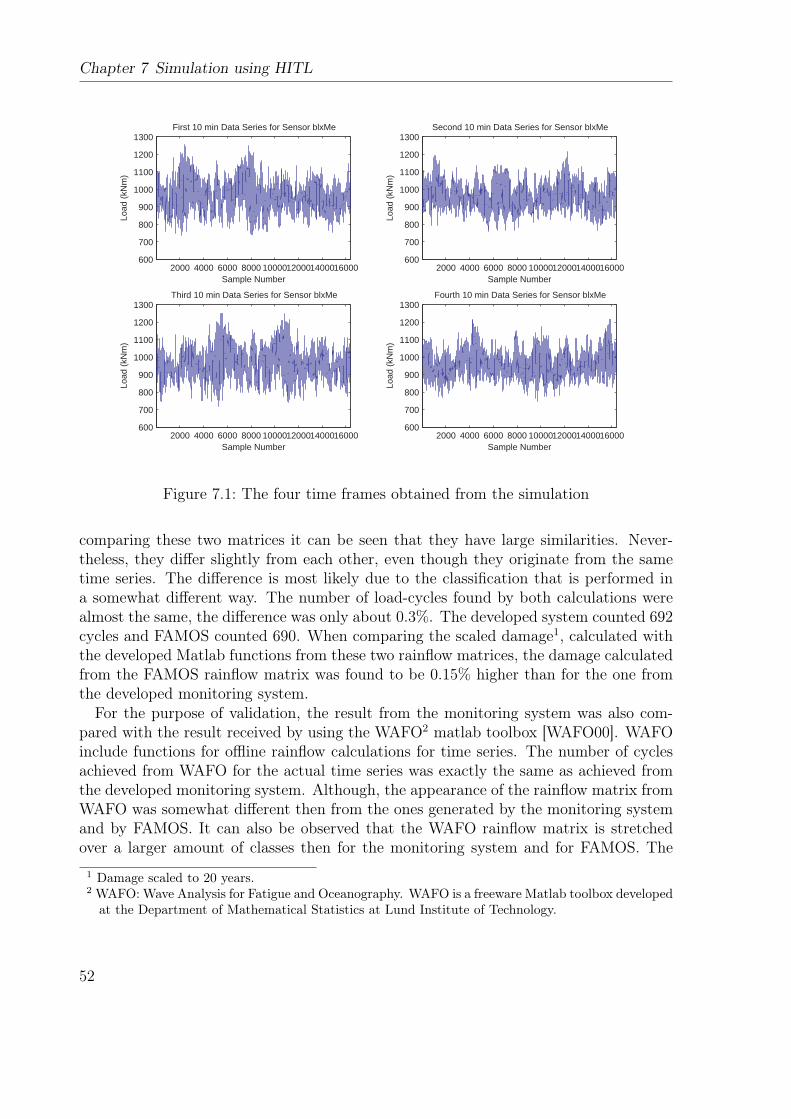
Chapter 7 Simulation using HITL
2000 4000 6000 8000 10000120001400016000600
700
800
900
1000
1100
1200
1300
Load
(kN
m)
Sample Number
First 10 min Data Series for Sensor blxMe
2000 4000 6000 8000 10000120001400016000600
700
800
900
1000
1100
1200
1300
Sample Number
Load
(kN
m)
Second 10 min Data Series for Sensor blxMe
2000 4000 6000 8000 10000120001400016000600
700
800
900
1000
1100
1200
1300
Sample Number
Load
(kN
m)
Third 10 min Data Series for Sensor blxMe
2000 4000 6000 8000 10000120001400016000600
700
800
900
1000
1100
1200
1300
Sample Number
Load
(kN
m)
Fourth 10 min Data Series for Sensor blxMe
Figure 7.1: The four time frames obtained from the simulation
comparing these two matrices it can be seen that they have large similarities. Never-theless, they differ slightly from each other, even though they originate from the sametime series. The difference is most likely due to the classification that is performed ina somewhat different way. The number of load-cycles found by both calculations werealmost the same, the difference was only about 0.3%. The developed system counted 692cycles and FAMOS counted 690. When comparing the scaled damage1, calculated withthe developed Matlab functions from these two rainflow matrices, the damage calculatedfrom the FAMOS rainflow matrix was found to be 0.15% higher than for the one fromthe developed monitoring system.
For the purpose of validation, the result from the monitoring system was also com-pared with the result received by using the WAFO2 matlab toolbox [WAFO00]. WAFOinclude functions for offline rainflow calculations for time series. The number of cyclesachieved from WAFO for the actual time series was exactly the same as achieved fromthe developed monitoring system. Although, the appearance of the rainflow matrix fromWAFO was somewhat different then from the ones generated by the monitoring systemand by FAMOS. It can also be observed that the WAFO rainflow matrix is stretchedover a larger amount of classes then for the monitoring system and for FAMOS. The
1 Damage scaled to 20 years.2 WAFO: Wave Analysis for Fatigue and Oceanography. WAFO is a freeware Matlab toolbox developed
at the Department of Mathematical Statistics at Lund Institute of Technology.
52
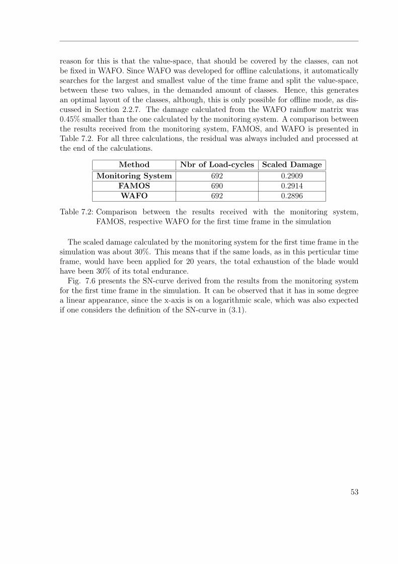
reason for this is that the value-space, that should be covered by the classes, can notbe fixed in WAFO. Since WAFO was developed for offline calculations, it automaticallysearches for the largest and smallest value of the time frame and split the value-space,between these two values, in the demanded amount of classes. Hence, this generatesan optimal layout of the classes, although, this is only possible for offline mode, as dis-cussed in Section 2.2.7. The damage calculated from the WAFO rainflow matrix was0.45% smaller than the one calculated by the monitoring system. A comparison betweenthe results received from the monitoring system, FAMOS, and WAFO is presented inTable 7.2. For all three calculations, the residual was always included and processed atthe end of the calculations.
Method Nbr of Load-cycles Scaled Damage
Monitoring System 692 0.2909FAMOS 690 0.2914WAFO 692 0.2896
Table 7.2: Comparison between the results received with the monitoring system,FAMOS, respective WAFO for the first time frame in the simulation
The scaled damage calculated by the monitoring system for the first time frame in thesimulation was about 30%. This means that if the same loads, as in this perticular timeframe, would have been applied for 20 years, the total exhaustion of the blade wouldhave been 30% of its total endurance.
Fig. 7.6 presents the SN-curve derived from the results from the monitoring systemfor the first time frame in the simulation. It can be observed that it has in some degreea linear appearance, since the x-axis is on a logarithmic scale, which was also expectedif one considers the definition of the SN-curve in (3.1).
53
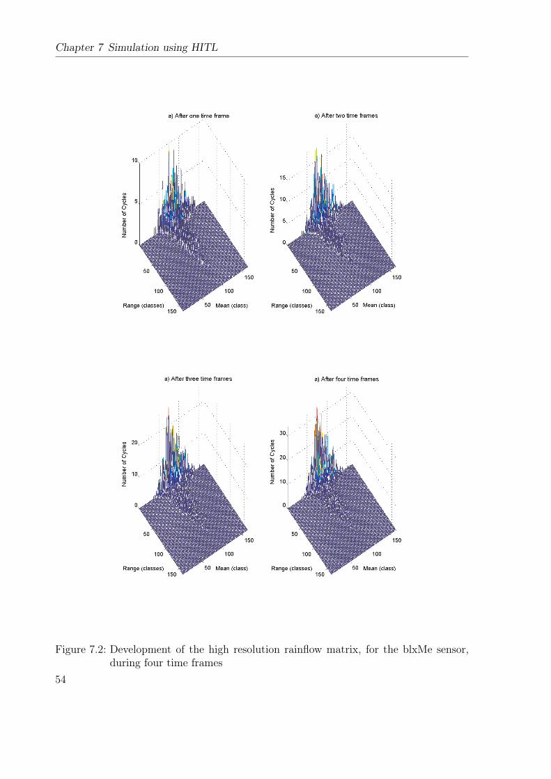
Chapter 7 Simulation using HITL
Figure 7.2: Development of the high resolution rainflow matrix, for the blxMe sensor,during four time frames
54

2040
6080
100120
140160
20
40
60
80
100
120
140
160
05
10
Mean (class)
Range (classes)
Num
ber
of C
ycle
s
Figure 7.3: High resolution rainflow matrix calculated by the monitoring system, usinginternal classification, for a time frame from the blxMe sensor
55

Chapter 7 Simulation using HITL
2040
6080
100120
140160
20
40
60
80
100
120
140
160
05
10
Mean (class)
Range (classes)
Num
ber
of C
ycle
s
Figure 7.4: Rainflow matrix calculated with the signal processing tool FAMOS, for atime frame from the blxMe sensor
56
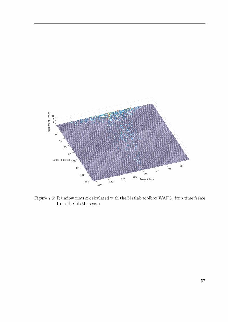
2040
6080
100120
140160
20
40
60
80
100
120
140
160
05
10
Mean (class)
Range (classes)
Num
ber
of C
ycle
s
Figure 7.5: Rainflow matrix calculated with the Matlab toolbox WAFO, for a time framefrom the blxMe sensor
57
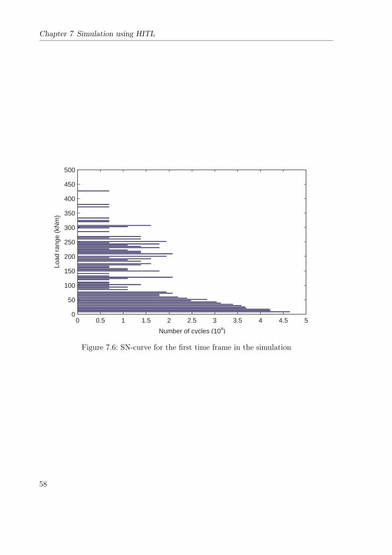
Chapter 7 Simulation using HITL
0 0.5 1 1.5 2 2.5 3 3.5 4 4.5 50
50
100
150
200
250
300
350
400
450
500
Number of cycles (10x)
Load
ran
ge (
kNm
)
Figure 7.6: SN-curve for the first time frame in the simulation
58
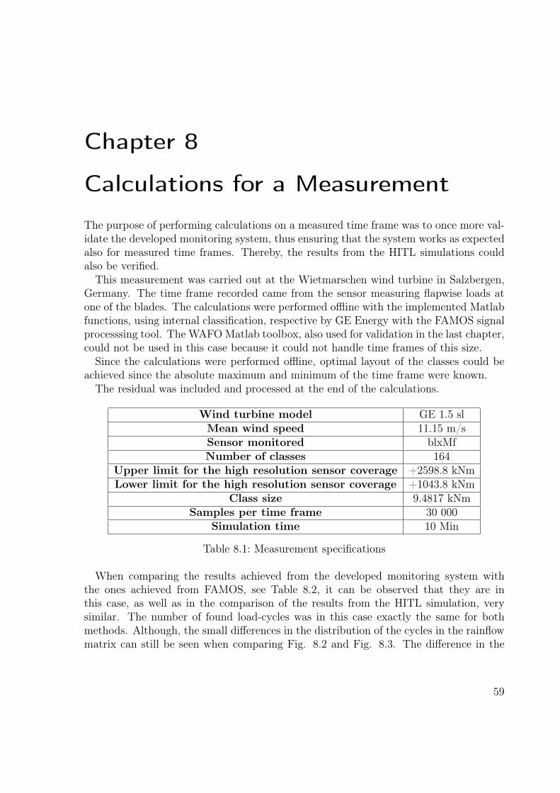
Chapter 8
Calculations for a Measurement
The purpose of performing calculations on a measured time frame was to once more val-idate the developed monitoring system, thus ensuring that the system works as expectedalso for measured time frames. Thereby, the results from the HITL simulations couldalso be verified.
This measurement was carried out at the Wietmarschen wind turbine in Salzbergen,Germany. The time frame recorded came from the sensor measuring flapwise loads atone of the blades. The calculations were performed offline with the implemented Matlabfunctions, using internal classification, respective by GE Energy with the FAMOS signalprocesssing tool. The WAFO Matlab toolbox, also used for validation in the last chapter,could not be used in this case because it could not handle time frames of this size.
Since the calculations were performed offline, optimal layout of the classes could beachieved since the absolute maximum and minimum of the time frame were known.
The residual was included and processed at the end of the calculations.
Wind turbine model GE 1.5 slMean wind speed 11.15 m/sSensor monitored blxMfNumber of classes 164
Upper limit for the high resolution sensor coverage +2598.8 kNmLower limit for the high resolution sensor coverage +1043.8 kNm
Class size 9.4817 kNmSamples per time frame 30 000
Simulation time 10 Min
Table 8.1: Measurement specifications
When comparing the results achieved from the developed monitoring system withthe ones achieved from FAMOS, see Table 8.2, it can be observed that they are inthis case, as well as in the comparison of the results from the HITL simulation, verysimilar. The number of found load-cycles was in this case exactly the same for bothmethods. Although, the small differences in the distribution of the cycles in the rainflowmatrix can still be seen when comparing Fig. 8.2 and Fig. 8.3. The difference in the
59
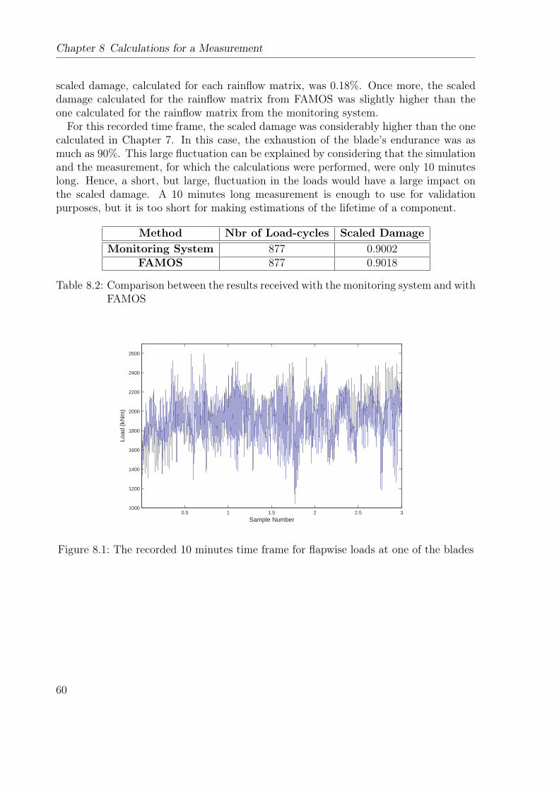
Chapter 8 Calculations for a Measurement
scaled damage, calculated for each rainflow matrix, was 0.18%. Once more, the scaleddamage calculated for the rainflow matrix from FAMOS was slightly higher than theone calculated for the rainflow matrix from the monitoring system.
For this recorded time frame, the scaled damage was considerably higher than the onecalculated in Chapter 7. In this case, the exhaustion of the blade’s endurance was asmuch as 90%. This large fluctuation can be explained by considering that the simulationand the measurement, for which the calculations were performed, were only 10 minuteslong. Hence, a short, but large, fluctuation in the loads would have a large impact onthe scaled damage. A 10 minutes long measurement is enough to use for validationpurposes, but it is too short for making estimations of the lifetime of a component.
Method Nbr of Load-cycles Scaled Damage
Monitoring System 877 0.9002FAMOS 877 0.9018
Table 8.2: Comparison between the results received with the monitoring system and withFAMOS
0.5 1 1.5 2 2.5 31000
1200
1400
1600
1800
2000
2200
2400
2600
Sample Number
Load
(kN
m)
Figure 8.1: The recorded 10 minutes time frame for flapwise loads at one of the blades
60

2040
6080
100120
140160
20
40
60
80
100
120
140
160
05
10
Mean (class)
Range (classes)
Num
ber
of C
ycle
s
Figure 8.2: High resolution rainflow matrix calculated by the monitoring system, usinginternal classification, for a time frame from the blxMf sensor
61

Chapter 8 Calculations for a Measurement
2040
6080
100120
140160
20
40
60
80
100
120
140
160
05
10
Mean (class)
Range (classes)
Num
ber
of C
ycle
s
Figure 8.3: Rainflow matrix calculated with the signal processing tool FAMOS, for atime frame from the blxMf sensor
62

Part III
Conclusions and Perspectives
63


Chapter 9
Summary
The aim of this thesis was to design and implement a lifetime monitoring system for theGE 1.5s/sl wind turbine. Knowing the estimated remaining lifetime makes it possible tochange the wind turbine components before they break. This increases both the securityand availability of the wind turbine.
The rainflow counting method was chosen for extraction of load cycles from the loadsequences. It has been shown best practice to use the rainflow counting method whenacquiring relevant information from a load sequence, to monitor the lifetime of a compo-nent. The rainflow counting method can also be used for online processing, which wasnecessary for this thesis.
The classification of the data points in the time frames were performed in a conser-vative manner. The conservative classification method was chosen before the least-errormethod in order to ensure that the damage calculated is always at least as large as inreality, in no case less.
To make online rainflow counting possible, a new approach had to be found for thelayout of the classes. By having two rainflow matrices, one with high resolution fora small value-space and one with low resolution for a large value-space, all necessaryinformation from the rainflow counting could be stored. This was also a very memoryefficient solution, demanding only a fraction of the memory needed for other possiblesolutions.
It was found that the life meter could be represented as the quotient between Seq
and Seq_max in order to present measured damage equivalent loads against the designedmaximum damage equivalent loads. The measured damage equivalent loads should bemultiplied with safety factors in order to ensure that the components do not break beforethey are expected to.
Two design approaches for the monitoring system were implemented. The first im-plementation was more time-efficient, and also more conservative, than the second onebecause the classification was performed before the rainflow counting. In the secondimplementation, the classification of the turning points was carried out internally in therainflow counting function block. This led to more accurate results, although, it wasalso more time consuming since a lower amount of data points were filtered out beforethe rainflow counting function block. By changing a parameter in the main program the
65

Chapter 9 Summary
user can decide which of the two implementations to use.All POU’s implemented were also translated into Matlab functions in order to be used
for offline validation purposes.The monitoring system was made robust to handle outer disturbances to the sensors
and/or to the data acquisition system by having an internal error-detector and an error-handler implemented. The error-detector can detect faults such as sensor failure ordiscontinuities in or between the incoming time frames.
The validation of the lifetime monitoring system was carried out by comparing withthe results achieved from the signal processing tool FAMOS and the Matlab toolboxWAFO. It turned out that the results matched each other very well. The differencein the results was always less then 0.5%. This difference was most probably due to adiscrepancy between the classification methodologies used by the different systems.
A prototype of the monitoring system was succesfully installed in the Holsten-BextenGE 1.5sle wind turbine in Salzbergen, Germany.
66

Chapter 10
Quality Assessments
During this thesis work, several simplifications and assumptions were, of course, made.These could make the results achieved less accurate, but are also often necessary sinceit is not feasible to perform empirical investigations for all unknown quantities. In thisthesis, assumptions on the value of a few quantities have been made. E.g. the number ofclasses being used in the classification of the data points in the time series was chosen tobe 164, because this had shown good practice by tests performed by GE Energy. It was aassumed that this number of classes was enough, although no own tests were performedfor comparison and validation. On the other hand, it was also of interest to choosesimilar parameters as the ones being used by GE Energy since it made comparison ofgenerated results possible. In this thesis, being able to do meaningful comparisons wasmore important than finding and using the optimal number of classes.
Another assumption was the position of the limits between the high resolution andlow resolution rainflow matrices. The resolution needed was only approximately known.A one month long monitoring of the loads on a real wind turbine was studied, and thetotal maximum and minimum load taking place during this time were used as limits forthe high resolution rainflow matrix. All loads beyond this value-space were consideredto be rare and therefore a lower resolution was used for these loads. Only the approxi-mate magnitude of these rare large loads was needed in order to be able to calculate afairly correct fatigue. The resolution of the low resolution matrix was set to a tenth ofthe resolution of the high resoution matrix. This makes the total covered value spaceprobably much larger than it would have to be. Although, it ensures that the reallyextreme loads will fit in the low resolution matrix.
To find accurate and unambiguous maximum DEL’s to use for the damage calculationswas not trivial. The maximum DEL’s had to be taken from a wind turbine with thesame specifications as the one where the life time monitoring took place. It was alsonecessary to use DEL’s that had been calculated for exactly the same positions as for themonitored sensors. The DEL’s used in this thesis were only given for different integervalues of the material parameter m (see section 3.1). To use only a integer-value for mwas an approximation since it is in reality a floating point value.
As mentioned in section 3.2, safety factors have to be multiplied to the total calculateddamage in order to be sure that components do not fail before they are expected to.
67

Chapter 10 Quality Assessments
The exact magnitude of these safety factors are not known and therefore such factorshave not been included in the damage calculations in this thesis. In order to find out thenecessary magnitude of the safety factors, several empirical tests have to be performed.
The differences between the results achieved with the, in this thesis, developed systemand the ones achieved from the FAMOS software respective WAFO Matlab functionsare most probably due to differences in the classification method used. Since the num-ber of cycles found by each application were almost the same, it suggests that therainflow counting operates in the same way in all these three methods. Although, thefinal fatigue calculated with the developed rainflow counter respective with the FAMOSsignal-processing tool was the same. This was the most essential result in this thesisand therefore it was of most importance that this validation turned out positive.
Whenever an approximation had to be made in the calculations in this thesis, it wasalways ensured that it was conservative. This was of high importance since the estimatedremaining lifetime of the components of a wind turbine is, for security reasons, never tobe higher than it really is.
68

Chapter 11
Future Work
The lifetime monitoring system has been designed and implemented in this thesis work.A prototype of it has been installed into a wind turbine. Future work will now consistof carrying out tests on the prototype system over a longer period of time, in order tocomplete verification. By doing this, it will become clear if the accuracy of the systemis satisfactory or if it has to be tuned in order to achieve long term reliability.
Multiplying the results with safety-factors has not been done in this thesis. This willalso have to be considered in the future. By performing tests over a longer period of time,and for several different wind turbines, the safety-factors needed can be determined.
With the developed system, it is now possible to monitor the lifetime of several com-ponents of a wind turbine. A future task will be to develop new controller strategies thattake use of the information that the monitoring system delivers in order to optimize theoperation of the wind turbine regarding the lifetime of the components and the energycapture.
69

Chapter 11 Future Work
70

Bibliography
[AGRB94] C. Amzallag, J.P. Gerey, J.L. Robert, J. Bahuaud: Standardization ofthe rainflow counting method for fatigue analysis, International Journalof Fatigue, Vol. 16, pp. 287-293, 1994
[DeJi03] S. Amarnath, A. Deshpande, P. Jindal: PP7 and Flex5 manual, version1.0, GE Wind Energy, 2003
[DoSo82] S.D. Downing, D.F. Socie: Simple rainflow counting algorithms, Interna-tional Journal of Fatigue, Vol. 4, pp. 31-40, 1982
[DrHa95] K. Dressler, M. Hack: Fatigue Lifetime Estimation on Rainflow CountedData Using the Local Strain Approach, 1995
[Echt96] A. T. Echtermeyer, et al.: Method to predict fatigue lifetimes of GRPwind turbine blades and comparison with experiments, European UnionWind Energy Conference, 1996
[Efun05] eFunda - Engineering Fundamentals, http://www.efunda.com/, accessdate 27/09/05
[Endo74] T. Endo: Proceedings from Symposium of Mechanical Behaviour of Ma-terials, Society of Material Science, Japan, 1974
[Feic05] W. Feichter: Real-time Monitoring for 1.5 Mega Watt Wind Turbine Gen-erators, Bachelor Thesis, Munich University of Applied Sciences, 2005
[Flei99] K. Fleischer: LaTeX - mehr als nur schreiben, Fernuniversität Hagen,1999
[Germ03] Richtlinie für die Zertifierung von Windenergieanlagen, GermanischerLloyd Wind Energie GmbH, Ausgabe 2003
[GEGR04] Hardware-in-the-loop Simulator for Wind Turbine Control, internal doc-ument, GE Global Research, Shanghai, 2004
[GEWE04] GEWE - 3.6 Standard Europe, GE Wind Energy GmbH, 2004
71

Bibliography
[GEWE05] ADC-Report, GE Wind Energy GmbH, 27 Revision, 2005
[Joha93] R. Johansson: System Modeling & Identification, Prentice-Hall Inc., 1993
[Joha99] P. Johansson: Modelling of Random Vehicle Fatigue Loads throughTransformed Gaussian Processed, Department of Mathematical Statis-tics, Lund Institute of Technology, 1999
[Johb99] P. Johansson: Rainflow Analysis of Switching Markov Loads, DoctoralThesis, Department of Mathematical Statistics, Lund Institute of Tech-nology, 1999
[JoSM05] P. Johannesson, T. Svensson, J. de Maré: Fatigue life prediction based onvariable amplitude tests - methodology, International Journal of Fatigue,2005
[Jürg95] M. Jürgens: LaTeX - eine Einführung und ein bisschen mehr..., Fernuni-versität Hagen, 1995
[Kopk04] H. Kopka: Guide to LaTeX, Addison-Wesley Publishing Company, 2004
[Lamp95] L. Lamport: Das LaTeX Handbuch, Addison-Wesley Publishing Com-pany, 1995
[MaKa05] A. Mangold, S. Kleinhansl: Load Assessment for the Wind Energy Tur-bine GE15sl, 1.5sl 50 Hz DIBt Zone II A LM37.3P2 100m, GE WindEnergy GmbH, 2005
[MaKb05] A. Mangold, S. Kleinhansl: Load Assessment for the Wind Energy Tur-bine GE15sl, 1.5sl 50 Hz IEC Type Class IIIA 7.5 m/s LM37.3P2 100m,GE Wind Energy GmbH, 2005
[Mine45] M. A. Miner: Cumulative damage in fatigue, Journal of Applied Mechan-ics, Vol. 12, pp. A159-A164, 1945
[NaAm03] A. Natarajan, S. Amarnath: Flex5 - Theory Manual, Version 1.0, GEWind Energy, 2003
[Palm24] A. Palmgren: Die Lebensdauer von Kugellagern, Zeitschrift des vereinsDeutscher Ingenieure, Vol. 68, pp. 339-41, 1924
[Rix00] P. Rix: Lastannahmen zur Enron Wind 1.5sl nach DIBt WZII, DiplomaThesis, Enron Wind GmbH, 2000
[Rych87] I. Rychlik: A new definition of the rainflow cycle counting method, Inter-national Journal of Fatigue, Vol. 9, pp. 119-121, 1987
72

Bibliography
[Suth95] H. J. Sutherland: Effect of Cyclic Stress Distribution Models on FatigueLife Predictions, SED, Vol. 16, ASME, pp. 83-90, 1995
[SöKR04] H. Söker, S. Kieselhorst, R. Royo, Load Monitoring on a Mainshaft, aCase Study, Proceedings from DEWEK, Wilhelmshafen, 2004
[WAFO00] The WAFO Group: A Matlab Toolbox for Analysis of Random Wavesand Loads, Department of Mathematical Statistics, Lund Institute ofTechnology, 2000
[WeZe88] A. Westermann-Friedrich, H. Zenner: Zählverfahren zur Bildung vonKollektiven aus Zeitfunktionen, FVA-Merkblatt, Vol. 0/14, 1988
[Wind03] Windkraftjournal, Allianz Versicherungs-AG, 3/2003
[Wind05] Positions of sensors installed on a GE 1.5sle at Bexten, WINDTESTKaiser-Wilhelm-Koog GmbH, 2005
73

Bibliography
74

Statutory Declaration
I do solemnly and sincerely declare that I have developed and written this enclosed Mas-ter Thesis completely by myself, and have not used sources or means without declarationin the text. Any thoughts from others, or literal quotations, are clearly marked. Thiswork has not been submitted to any other examining authority and has not yet beenpublished.
Garching, 31. October 2005
75
