1

LightAMC: Lightweight Automatic ModulationClassification via Deep Learning and Compressive

SensingYu Wang, Student Member, IEEE, Jie Yang, Member, IEEE, Miao Liu, Member, IEEE, and

Guan Gui, Senior Member, IEEE

Abstract—Automatic modulation classification (AMC) is anpromising technology for non-cooperative communication sys-tems in both military and civilian scenarios. Recently, deeplearning (DL) based AMC methods have been proposed with out-standing performances. However, both high computing cost andlarge model sizes are the biggest hinders for deployment of theconventional DL based methods, particularly in the applicationof internet-of-things (IoT) networks and unmanned aerial vehicle(UAV)-aided systems. In this correspondence, a novel DL basedlightweight AMC (LightAMC) method is proposed with smallermodel sizes and faster computational speed. We first introduce ascaling factor for each neuron in convolutional neural network(CNN) and enforce scaling factors sparsity via compressivesensing. It can give an assist to screen out redundant neurons andthen these neurons are pruned. Experimental results show thatthe proposed LightAMC method can effectively reduce modelsizes and accelerate computation with the slight performanceloss.

Index Terms—Lightweight automatic modulation classification(LightAMC), convolutional neural network (CNN), neuron prun-ing, compressive sensing.

I. INTRODUCTION

Automatic modulation classification (AMC) is a novel andpromising technology in the non-cooperative communicationscenarios with neither agreement nor authorization betweenthe transmitters and the receivers. The AMC methods havevarious applications in military and civilian fields, includingintercepted signal recovering or spectrum monitoring [1]–[3].There are two typical AMC methods based on features andlikelihood functions, respectively. This paper focuses on thefeature-based AMC method, which can be modeled as a pat-tern recognition problem based on extracted features withoutany prior information. Typical manmade features include highorder statistical features, wavelet transform-based features andso on.

In recent years, deep learning (DL) has been consideredone of the most effective tools to solve various problems

This work was supported by the Project Funded by the National Scienceand Technology Major Project of the Ministry of Science and Technology ofChina under Grant TC190A3WZ-2, the Jiangsu Specially Appointed Professorunder Grant RK002STP16001, the Innovation and Entrepreneurship of JiangsuHigh-level Talent under Grant CZ0010617002, the Six Top Talents Program ofJiangsu under Grant XYDXX-010, the 1311 Talent Plan of Nanjing Universityof Posts and Telecommunications. (Corresponding author: Guan Gui.)

The authors are with the College of Telecommunications and Infor-mation Engineering, Nanjing University of Posts and Telecommunica-tions, Nanjing 210003, China (E-mails: {1018010407, jyang, liumiao,guiguan}@njupt.edu.cn).

in wireless communications [4]–[14], because of its powerfulfeature extraction capability, especially confronting with high-dimensional data. At the same time, many DL-based AMCmethods were proposed for the higher classification perfor-mances. T. O’Shea et al. proposed a convolutional neuralnetwork (CNN)-based AMC method using the in-phase andquadrature (IQ) component of signals [15]. S. Rajendran etal. proposed a novel data-driven automatic modulation classi-fication based on the long short term memory (LSTM) [16].What’ more, S. Hu, et al. [17] demonstrated the robustnessof DL-based AMC method in more complex noise conditions,including white non-Gaussian noise and time-correlated non-Gaussian noise. However, DL models generally have largemodel sizes and slow computation speed. Thus, it is difficultto apply these methods into the edge devices [18]–[21],such as internet-of-thing (IoT) devices and unmanned aerialvehicle (UAV), which are equipped with the limited devicememories and computation capability. Hence, the compressionand acceleration of DL models are necessary in the futuredevelopment of the DL-based wireless communications.

In this paper, we propose a compressive sensing (CS)-basedneuron pruning technology to implement the lightweight AMC(LightAMC) method. Specifically, the proposed method isimplemented by pruning redundant neurons via `1 regulariza-tion on the fundament of the mixed dataset-based AMC (M-AMC) method. Experimental results are given to confirm theproposed method in terms of the model sizes, the computationtime as well as the classification performance.

II. SIGNAL MODEL AND PROBLEM FORMULATION

Consider that the received signal y = {y(k)}Kk=1 is acomplex-valued baseband signal, and its sampling strictlyfollows Nyquist criterion. The signal in the k-th samplingmoment can be expressed by

y(k) = Aejϕs(k) + w(k), (1)

where s(k) is a modulation signal, and the energy of modula-tion signal is normalized for the fair classification of differentmodulation types, i.e.,

∑Kk=1 |s(k)|2 = 1; w(k) is zero-mean

additive white Gaussian noise (AWGN). In addition, A and ϕare the channel gain and the phase offset, respectively. Thesetwo parameters are constant under the assumption of the flatfading and time-invariant channel.

2

Based on the signal model, two independent datasets areprepared for the training and testing of the CNN. The sam-ple in the datasets consists of the in-phase and quadrature(IQ) component of the received signal. The IQ componentalso represents real part and imaginary part of the receivedsignal, respectively. Thus, I = {real[y(k)]}Kk=1, and Q ={imag[y(k)]}Kk=1. Then, the IQ sample can be written as

IQ =

{real[y(k)]

imag[y(k)]

}Kk=1

, (2)

and it is a 2 × K real-valued matrix. Then, we specificallydescribe the problem of AMC. AMC is a technique to blindlyidentify modulation types in the range of a limited modulationtype candidate pool Θ = {θi}Mi=1, where θi is one ofthe modulation types. According to the maximum-a-posterior(MAP) criterion, this problem can be described as

θi = arg maxθi∈Θ

P (θi|y), (3)

where P (θi|y) is the probability distribution function (PDF)of θi under the condition of the received signal y. Without theloss of generality, we consider two modulation type candidatepools, i. e., Θ1 = {BPSK, QPSK, 8PSK} [22], [23] and Θ2 ={BPSK, QPSK, 8PSK, 16QAM} [1], [17].

III. EXISTING AMC METHODS

A. Traditional AMC Method Based on HOC and SVM

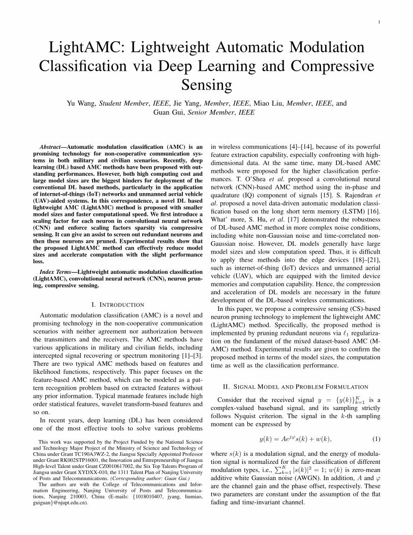
The architecture of the traditional method is depicted inFig. 1. It consists of pre-processing, feature extraction, clas-sifier, and SNR estimation. Pre-processing contains signalconversion, frequency and phase synchronization and so on.Feature extraction is the core step of the AMC method andwe consider the fourth order cumulants as features [22]. Forthe received baseband complex signal y = {y(k)}Kk=1, the i-th order moment is defined as Mij = E[yi−jy∗j ]. Then, thefourth-order cumulants [22] are defined as

C40 = M40 − 3M220, (4)

C41 = M41 − 3M21M20, (5)

C42 = M42 − |M20|2 − 2M221. (6)

In the actual applications, the number of the sampling pointsfor the received signal y is limited. Hence, the estimation valueof i-th order moments Mij = 1

K

∑Kk=1[yi−j(k)y∗j(k)] is ap-

plied to replace the theoretical value. Similarly, the estimationvalue of fourth-order cumulants C4j , j ∈ {0, 1, 2} can beobtained by replacing Mij in (4–6) with Mij . Considering thescale problem, the estimation value of fourth-order cumulantsis generally normalized, and the normalized value of fourth-order cumulants [23] is

C4j =C4j

1K (∑Kk=1 |y(k)|2)2

,where j ∈ {0, 1, 2}, (7)

and {C4j}2j=0 is a feature vector for training SVM to classifydifferent modulation signals. In addition, SVM is applied forthe module “Classification”, and multiple SVM models mustbe prepared for the varying SNR conditions. What’s more, it is

TABLE ITHE STRUCTURE OF CNN, INCLUDING LAYER NUMBER, LAYER TYPE AND

LAYER STRUCTURE.

NO. Type Structure- - Input (IQ samples, labels)1 Conv Conv2D (u1, 1× 8) + BN + ReLU + Dropout (0.05)2 Conv Conv2D (u2, 2× 4) + BN + ReLU + Dropout (0.05)3 FC Dense (u3) + BN + ReLU + Dropout (0.5)4 FC Dense (u4) + BN + ReLU + Dropout (0.5)5 FC Dense (M ) + Softmax

Tips: “Conv” represents the convolutional layer and ”FC” is the fully-connected layer.

necessary to estimate the real-time SNR via the module “SNRestimation” to choose the suitable SVM model from multipleSVM models for the correct classification.

Unknown

Signal

SNR

estimation

Modulation

Type

Pre-

processing

Choose classifier model with

corresponding SNR

Feature

ExtractionClassification

Fig. 1. The architecture of feature-based AMC method. The key steps ofAMC method are feature extraction and classification. In the traditional AMCmethod, HOC is applied to characterize the difference of various modulationtypes, while SVM is as a classifier. In the F-AMC method, CNN is both thefeature extractor and classifier. What’s more, SNR estimation gives an assistto choose corresponding SVMs or CNNs, because SVM or CNN in thesepreviously proposed methods is trained on the IQ samples with the fixedSNR, and they can just be adopted into the corresponding SNR.

B. CNN-based F-AMC Methods

CNN-based AMC methods have the similar architecturewith the traditional AMC method, and the only differenceis that HOC and SVM is replaced by CNN. Existing CNN-based AMC methods consider the training CNN model onfixed samples with single SNR. Here, it is referred as theF-AMC method. The architecture of the F-AMC method isshown in Fig. 1, where CNN is applied to replace the modulesof “Feature Extraction” and “Classification”.

IV. THE PROPOSED LIGHTAMC METHOD

Our proposed CNN-based LightAMC method is introducedin this section. A novel neuron pruning technology based on `1regularization is applied to realize the LightAMC method. Theimplementation of the LightAMC method consists of training,pruning and finetuning.

A. CNN Training for M-AMC Method

Training is to train a CNN, designed by the artificialexperiences, to classify the modulation signals. In the F-AMCmethods [1], [15], [17], CNN is trained on the fixed SNR, andthey are only useful for the IQ samples with the correspondingSNR. It means that the SNR estimation is necessary for thechoice of the suitable CNN model, which is shown in Fig.1. In addition, the F-AMC methods have the weak robustnessunder varying noise condition.

3

Unlike the F-AMC methods, the M-AMC method is pro-posed with the capability to confront with the varying noisecondition without the assist of the SNR estimation. BecauseM-AMC method is trained on the mixed datasets with multipleSNRs, and the CNN can extract more robust and generalfeatures from mixed dataset. Assuming that SNR is from -10dB to 10 dB, we use multiple IQ samples with different SNRs(it ranges from -10 dB to 10 dB with 2 dB as an interval) andmix them equally to create the mixed dataset for training.

In addition, for the fair comparison of the F-AMC and M-AMC method, we consider to apply the same CNN structureinto both F-AMC and M-AMC method, which is shown inTab. I. This CNN has five layers, containing two convolutionallayers and three fully-connected layers. In first four layers,the numbers of neurons are denoted as {ul}4l=1, which isequal to {128, 64, 256, 128}, and rectified linear unit (ReLU )fReLU (·) = max(·, 0) is as the activation function for thesefour layers. The number of neurons in the last layer is decidedby the number of modulation types M , and Softmax is theactivation function for the last layer.

Original Network Structure Lightweight Network Structure

The l-th

layer

×

…

The l-th

scaling factor layer

×

×

×

×

…

The (l+1)-th

layer

…

The l-th

layer

×

…

The l-th

scaling factor layer

×

×

…

The (l+1)-th

layer

…

-norm

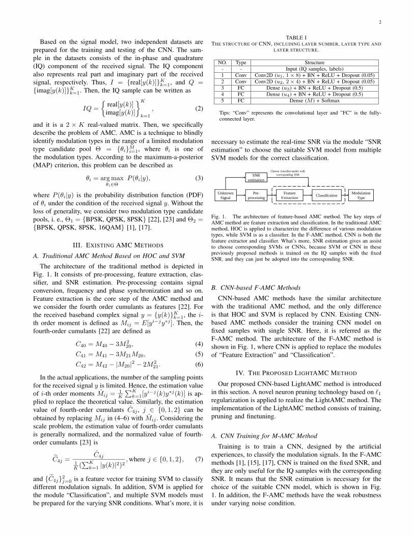
Fig. 2. The principle of neuron pruning based on `1 regularization.

B. Neuron Pruning via `1 Regularization

Pruning is to cut down unimportant neurons, and how tomeasure the importance of neurons is critical. Inspired by [24][25], we introduce a learnable metrics α = {αl}4l=1 based on`1 regularization for this problem. α represents the scalingfactor, and it is multiplied by the output of each neuron in thefirst four layers of CNN. Hence, the output of one of the firstfour layers in CNN can be represented by

xl+1 = αl ·max{γl ·BNµl,σl,εl(Wl ∗ xl) + βl, 0}, (8)

where xl and xl+1 is the input and output, and W l, γl andβl are the trainable weight. In addition, BNµl,σl,εl(zin) =zin−µl√(σl)2+εl

, where µl = E(zin), (σl)2 = V ar(zin) and εl is a

minimum value to prevent that σl is zero.Then, we jointly train trainable parameters: W = {W l}5l=1,

γ = {γl}4l=1 and β = {βl}4l=1, and scaling factor α ={αl}4l=1 with sparsity constraint. Finally, we prune the neu-rons, whose scaling factor is smaller than threshold λthre.please notice that λthre = {λlthre}4l=1 is layered, and weusually set the 80% of the average value of all elements as the

threshold [24], but the detailed threshold is chosen by manytrying and testing on the validation samples as few neurons andas low validation performance loss as possible. The principleof neuron pruning is shown in Fig. 2. It is noted that the lossfunction is different and it is give as

arg maxW,γ,β,α

∑(x,y)

l(f(x;W,γ, β), y) + λ

4∑l=1

||αl||1, (9)

where (x, y) is training sample and label. The first term in(9) represents experience loss and we apply cross entropy lossfunction as this term. The second term is sparsity-inducingpenalty, and we choose `1 regularization, which is widelyapplied into achieve sparsity [26]. In addition, λ is utilizedto balance the two terms.

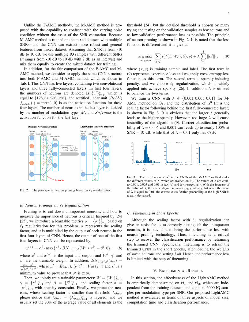
We train a CNN with λ ∈ {0.001, 0.005, 0.01} for M-AMC method on Θ1, and the distribution of α3 (it is thescaling factor following behind the first fully-connected layer)is shown in Fig. 3. It is obvious that the larger λ generallyleads to the higher sparsity. However, too large λ will causeinstability of the algorithm (9). Correct classification proba-bility of λ = 0.005 and 0.001 can reach up to nearly 100% atSNR = 10 dB, while that of λ = 0.01 only has 67%.

(a)

(b)

(c)

Fig. 3. The distribution of α3 in the CNNs of the M-AMC method underthe different values of λ, which are trained on θ1. The values of λ are equalto 0.001, 0.005 and 0.01 in (a), (b) and (c), respectively. With the increase ofthe value of λ, the sparse degree is increasing gradually, but when the valueof λ is equal to 0.01, the correct classification probability at the high SNR isgreatly decreased.

C. Finetuning in Short Epochs

Although the scaling factor with `1 regularization cangive an assist for us to correctly distinguish the unimportantneurons, it is inevitable to bring the performance loss withneuron pruning technology. Thus, finetuning is a criticalstep to recover the classification performance by retrainingthe trimmed CNN. Specifically, finetuning is to retrain thetrimmed CNN in the short epochs, after loading the weightsof saved neurons and setting λ=0. Hence, the performance lossis limited with the step of finetuning.

V. EXPERIMENTAL RESULTS

In this section, the effectiveness of the LightAMC methodis empirically demonstrated on Θ1 and Θ2, which are inde-pendent from the training datasets and contains 6000 IQ sam-ples per modulation type per SNR. Our proposed LightAMCmethod is evaluated in terms of three aspects of model size,computation time and classification performance.

4

Algorithm 1 The proposed LightAMC method.Input: IQ samples with SNRs ranging from −10 dB to 10 dB with

1 dB as an interval, and 6000 IQ samples per modulation typeper SNR;

Output: The CNN for LightAMC;1: Choose IQ samples with SNR = {−10,−8, · · · , 8, 10} dB and

mix these samples proportionally;2: Divide randomly the mixed samples into training samples and

validation samples by 7 : 3;3: Construct CNN according to Tab. I and introduce scaling factor{αl}4l=1 multiplied by the output of each neurons in the first fourlayers in CNN;

4: Set a proper λ (λ = 0.005 for Θ1 and λ = 0.006 for Θ2),choose stochastic gradient descent (SGD) as optimizer and trainCNN to minimize loss function (9);

5: Set a proper threshold λthre for each layer, and cut downneurons, whose corresponding scaling factor is smaller thanthreshold;

6: Set five retraining epochs, load the weights of the unprunedneurons and retrain the trimmed CNN on training samples torecover its performance;

7: return CNN.

TABLE IISTRUCTURES AND MODEL SIZES OF THREE CNN-BASED METHODS IN Θ1 .

Method {ul}4l=1 Model size (MB)F-AMC {128,64,256,128} 15.5×21M-AMC {128,64,256,128} 15.5

Traditional AMC - -LightAMC (Proposed) {77,18,49,44} 1.0 (93.5% ↓)

A. Model Size and Device Memory

The most obvious improvement of the LightAMC methodis that it has smaller sizes and requires fewer device memoriesthan F-AMC method, which is shown in Tabs. II–III. Theimprovement is beneficial from not only the application of M-AMC method but also the implementation of neuron pruningtechnology. When SNR ranges from −10 dB to 10 dB with 1dB as an interval, we need to train twenty-one CNN modelsfor F-AMC method, but only one CNN model is required inM-AMC method, benefitting from the application of mixeddatasets. So, considering that the same CNN structure isapplied into F-AMC and M-AMC method, CNN model sizesare same, but required device memories for M-AMC are only1/21 of that for F-AMC method.

One the basis of M-AMC method, LightAMC method isto prune unimportant neurons of CNN. The trimmed CNNstructure is shown in Tabs. II–III, and the number of neuronsfor each layer, especially two fully-connected layers, has beenreduced greatly. With the reduction of neurons, the CNN mod-el sizes and the required device memories are also decliningsharply. Specifically, CNN model sizes of LightAMC methodonly has 6.5% of that of M-AMC method in Θ1, and the ratiois 8.4% in Θ2. In addition, we do not compare CNN-basedAMC method with traditional AMC method, because the SVMin traditional AMC method is “Scikit-learn” as backend andthe CNN is based on “Keras”. Hence, it is meaningless tocompare these two kinds of AMC methods in the model sizes.

TABLE IIISTRUCTURES AND MODEL SIZES OF THREE CNN-BASED METHODS IN Θ2 .

Method {ui}4l=1 Model size (MB)F-AMC {128,64,256,128} 15.5×21M-AMC {128,64,256,128} 15.5

Traditional AMC - -LightAMC (Proposed) {81, 19, 63, 49} 1.3 (91.6% ↓)

B. Computation Time

The computation time of different AMC methods is depictedin Fig. 4. For the fair comparison, we test the computation timeon the same device equipped with i7-8750H and GTX1080Ti,and coding is based on python. It can be observed thatthe LightAMC method is faster than F-AMC and M-AMCmethod, because pruning the redundant neurons leads to thereduction of the redundant computation. Since F-AMC and M-AMC method have the same structure, hence the computationtime of which are 44.2 µs per sample. While the computationtime of the LightAMC method decreases by almost 24%,which is 33.2 µs per sample in Θ1 and 33.6 µs per sample inΘ2. Unlike these CNN-based methods, it is difficult to runtraditional AMC method on GPU. Hence, the computationtime of traditional AMC method is running on CPU, and it isobviously slower than these CNN-based methods.

Fig. 4. The average computation time of per sample in the different AMCmethods.

C. Classification Performance

Correct classification probability (Pcc = {P icc}10i=−10) is

applied to measure performance and it is given as

P icc =SicorrectStotal

, (10)

where Sicorrect is the number of correctly classified samplesunder SNR = i dB and Stotal is 18000 in Θ1 or 24000 in Θ2.The curve of Pcc is shown in Fig. 5.

While compressing model size and reducing the compu-tation time, the pruned LightAMC method has almost 10%performance gap with other CNN-based AMC methods, and itsperformance is still higher than the traditional AMC method.However, after a short term finetuning, the gap is extremely

5

reduced. The finetuned LightAMC method has the similarperformance with the M-AMC method, and it has the limitedperformance loss, compared with the F-AMC method.

(a)

(b)

Fig. 5. The classification performance of different AMC methods. (a) is theperformance in Θ1, (b) is the performance in Θ2.

VI. CONCLUDING REMARKS

In this correspondence, we have proposed an effectiveLightAMC method using CNN and compressive sensing undervarying noise regimes. The proposed LightAMC method isbased on the M-AMC method that is trained on mixed datasetwith multiple SNRs. Then, `1 regularization-based neuronpruning technology is applied to cut down redundant neuronsin the CNN for the M-AMC method. Hence, the proposedLightAMC method requires fewer device memories and hasfaster computational speed under the limited performance loss.Simulation results also demonstrate the superiority of the Ligh-tAMC method. In the future work, we will consider iterativeshrinkage-thresholding algorithm (ISTA) as the optimizer toreplace SGD for LightAMC method with `1 regularization,and we expect that ISTA-based LightAMC method can achievethe better performance.

REFERENCES

[1] F. Meng, et al., “Automatic modulation classification: A deep learnin-genabled approach,” IEEE Trans. Veh. Technol., vol. 67, no. 11, pp.10760–10772, 2018.

[2] I. Bisio, C. Garibotto, F. Lavagetto, and A. Sciarrone, “Outdoor places ofinterest recognition using WiFi fingerprints,” IEEE Trans. Veh. Technol.,vol. 68, no. 5, pp. 5076-5086, 2019.

[3] I. Bisio, C. Garibotto, F. Lavagetto, A. Sciarrone , S. Zappatore, “Blinddetection: Advanced techniques for WiFi-based drone surveillance,”IEEE Trans. Veh. Technol., vol. 68, no. 1, pp. 938–946, 2019.

[4] Z. Md. Fadlullah, et al., “State-of-the-art deep learning: Evolving ma-chine intelligence toward tomorrow’s intelligent network traffic controlsystems,” IEEE Commun. Surveys and Tuts., vol. 19, no. 4, pp. 2432-2455, 2017.

[5] N. Kato, et al., “The deep learning vision for heterogeneous networktraffic control: Proposal, challenges, and future perspective,” IEEE Wirel.Commun. Mag., vol. 24, no. 3, pp. 146–153, 2016.

[6] G. Gui, et al., “Deep learning for an effective nonorthogonal multipleaccess scheme,” IEEE Trans. Veh. Technol., vol. 67, no. 9, pp. 8440–8450, 2018.

[7] H. Huang, et al., “Deep learning for physical-Layer 5G wireless tech-niques: Opportunities, challenges and solutions,” IEEE Wirel. Commun.,to be published, doi: 10.1109/MWC.2019.1900027.

[8] G. Gui, F. Liu, J. Sun, J. Yang, Z. Zhou, D. Zhao, “Flight delayprediction based on aviation big data and machine learning,” IEEE Trans.Veh. Technol., doi: 10.1109/TVT.2019.2954094.

[9] H. Huang, et al., “Fast beamforming design via deep learning,” IEEETrans. Veh. Technol., to be published, doi: 10.1109/TVT.2019.2949122.

[10] Z. Md. Fadlullah, et al., “On intelligent traffic control for large-scaleheterogeneous networks: A value matrix-based deep learning approach,”IEEE Commun. Lett., vol. 22, no. 12, pp. 2479–2482, 2018.

[11] F. Tang, et al., “An intelligent traffic load prediction-based adaptivechannel assignment algorithm in SDN-IoT: A deep learning approach,”IEEE Internet Things J., vol. 5, no. 6, pp. 5141–5154, 2018.

[12] H. Huang, et al., “Deep-learning-based millimeter-wave massive MIMOfor hybrid precoding,” IEEE Trans. Veh. Technol., vol. 68, no. 3, pp.3027–3032, 2019.

[13] Z. Md. Fadlullah, et al., “Value iteration architecture based deep learningfor intelligent routing exploiting heterogeneous computing platforms,”IEEE Trans. Computers, vol. 68, no. 6, pp. 939–950, 2019.

[14] Y. Wang, et al., “Data-driven deep learning for automatic modulationrecognition in cognitive radios,” IEEE Trans. Veh. Technol., vol. 68, no.4, pp. 4074–4077, 2019.

[15] T. O’Shea and J. Hoydis, “An introduction to deep learning for thephysical layer,” IEEE Trans. Cogn. Commun. Netw., vol. 3, no. 4, pp.563–575, 2017.

[16] S. Rajendran et al., “Deep learning models for wireless signal classifi-cation with distributed low-cost spectrum sensors,” IEEE Trans. Cogn.Commun. Netw., vol. 4, no. 3, pp. 433–445, 2018.

[17] S. Hu, et al., “Deep neural network for robust modulation classificationunder uncertain noise conditions,” IEEE Trans. Veh. Technol., to bepublished, doi: 10.1109/TVT.2019.2951594.

[18] Z. Zhou, et al., “Access control and resource allocation for M2Mcommunications in industrial automation,” IEEE Trans. Ind. Informat.,vol. 15, no. 5, pp. 3093–3103, 2019.

[19] M. Liu, et al., “Deep cognitive perspective: resource allocation forNOMA based heterogeneous IoT with imperfect SIC,” IEEE InternetThings J., vol. 6, no. 2, pp. 2885–2894, 2019.

[20] Z. Zhou, et al., “Energy-efficient resource allocation for D2D communi-cations underlaying cloud-RAN-based LTE-A networks,” IEEE InternetThings J., vol. 3, no. 3, pp. 428–438, 2016.

[21] F. Tang, et al., “AC-POCA: Anti-coordination game based partiallyoverlapping channels assignment in combined UAV and D2D basednetworks,” IEEE Trans. Veh. Technol., vol. 67, no. 2, pp. 1672–1683,2018.

[22] A. Swami, B. M. Sadler, “Hierarchical digital modulation classificationusing cumulants,” IEEE Trans. Commun., vol. 48, no. 3, pp. 416–429,2000.

[23] K. Hassan, et al.,“Blind digital modulation identification for spatially-correlated MIMO systems,” IEEE Trans. Wirel. Commun., vol. 11, no.2, pp. 683–693, 2011.

[24] Z. Liu, et al., “Learning efficient convolutional networks through net-work slimming,” in ICCV, Venice, Italy, Oct. 22–29, 2017, pp. 2736–2744.

[25] J. Ye, et al., “Rethinking the smaller-norm-less-informative assumptionin channel pruning of convolution layers,” in ICLR, Vancouver, Canada,Apr. 30–May 3, 2018, pp. 1–11.

[26] Y. Li, et al., “Nonconvex penalized regularization for robust sparserecovery in the presence of SαS noise,” IEEE Access, vol. 6, no. 1,pp. 25474–25485, 2018.