lightcuts: a scalable approach to illuminationbjw/lightcuts.pdflightcuts: a scalable approach to...

To appear in the ACM SIGGRAPH conference proceedings

Lightcuts: A Scalable Approach to Illumination

Bruce Walter Sebastian Fernandez Adam Arbree Kavita Bala Michael Donikian Donald P. GreenbergProgram of Computer Graphics, Cornell University∗

Abstract

Lightcuts is a scalable framework for computing realistic illumina-tion. It handles arbitrary geometry, non-diffuse materials, and illu-mination from a wide variety of sources including point lights, arealights, HDR environment maps, sun/sky models, and indirect illu-mination. At its core is a new algorithm for accurately approximat-ing illumination from many point lights with a strongly sublinearcost. We show how a group of lights can be cheaply approximatedwhile bounding the maximum approximation error. A binary lighttree and perceptual metric are then used to adaptively partition thelights into groups to control the error vs. cost tradeoff.

We also introduce reconstruction cuts that exploit spatial coherenceto accelerate the generation of anti-aliased images with complex il-lumination. Results are demonstrated for five complex scenes andshow that lightcuts can accurately approximate hundreds of thou-sands of point lights using only a few hundred shadow rays. Re-construction cuts can reduce the number of shadow rays to tens.

CR Categories: I.3.7 [Computer Graphics]: Three-DimensionalGraphics and Realism—Color, shading, shadowing, and texture;Keywords: many lights, raytracing, shadowing

1 Introduction

While much research has focused on rendering scenes with com-plex geometry and materials, less has been done on efficiently han-dling large numbers of light sources. In typical systems, render-ing cost increases linearly with the number of lights. Real worldscenes often contain many light sources and studies show that peo-ple generally prefer images with richer and more realistic lighting.In computer graphics however, we are often forced to use fewerlights or to disable important lighting effects such as shadowing toavoid excessive rendering costs.

The lightcuts framework presents a new scalable algorithm for com-puting the illumination from many point lights. Its rendering cost isstrongly sublinear with the number of point lights while maintain-ing perceptual fidelity with the exact solution. We provide a quickway to approximate the illumination from a group of lights, andmore importantly, cheap and reasonably tight bounds on the max-imum error in doing so. We also present an automatic and locallyadaptive method for partitioning the lights into groups to control thetradeoff between cost and error. The lights are organized into a lighttree for efficient partition finding. Lightcuts can handle non-diffusematerials and any geometry that can be ray traced.

Having a scalable algorithm enables us to handle extremely largenumbers of light sources. This is especially useful because manyother difficult illumination problems can be simulated using the il-lumination from sufficiently many point lights (e.g., Figure 1). We

∗email: {bjw,spf,arbree,kb,mike,dpg}@graphics.cornell.edu

Figure 1: Bigscreen model: an office lit by two overhead area lights,two HDR flat-panel monitors, and indirect illumination. Our scal-able framework quickly and accurately computed the illuminationusing 639,528 point lights. The images on the monitors were alsocomputed using our methods: lightcuts and reconstruction cuts.

demonstrate three examples: illumination from area lights, fromhigh dynamic range (HDR) environment maps or sun/sky models,and indirect illumination. Unifying different types of illuminationwithin the lightcuts framework has additional benefits. For exam-ple, bright illumination from one source can mask errors in approx-imating other illumination, and our system automatically exploitsthis effect.

A related technique, called reconstruction cuts, exploits spatial co-herence to further reduce rendering costs. It allows lightcuts to becomputed sparsely over the image and intelligently interpolates be-tween them. Unlike most interpolation techniques, reconstructioncuts preserve high frequency details such as shadow boundaries andglossy highlights. Lightcuts can compute the illumination frommany thousands of lights using only a few hundred shadow rays.Reconstruction cuts can further reduce this to just a dozen or so.

The rest of the paper is organized as follows. We discuss previ-ous work in Section 2. We present the basic lightcuts algorithm inSection 3, give details of our implementation in Section 4, discussdifferent illumination applications in Section 5, and show lightcutresults in Section 6. Then we describe reconstruction cuts in Sec-tion 7 and demonstrate their results in Section 8. Conclusions are inSection 9. Appendix A gives an optimization for spherical lights.

2 Previous Work

There is a vast body of work on computing illumination and shad-ows from light sources (e.g., see [Woo et al. 1990; Hasenfratz et al.2003] for surveys). Most techniques accelerate the processing ofindividual lights but scale linearly with the number of lights.

Several techniques have dealt explicitly with the many lights prob-lem. [Ward 1994] sorts the lights by maximum contribution andthen evaluates their visibility in decreasing order until an error

1

Lightcuts: A Scalable Approach to Illumination, Walter et. al., SIGGRAPH 2005 2

bound is met. We will compare lightcuts with his technique in Sec-tion 6. [Shirley et al. 1996] divide the scene into cells and for eachcell split the lights into important and unimportant lists with thelatter very sparsely sampled. This or similar Monte Carlo tech-niques can perform well given sufficiently good sampling proba-bility functions over the lights, but robustly and efficiently com-puting these functions for arbitrary scenes is still an open problem.[Paquette et al. 1998] present a hierarchical approach using lighttrees similar to the ones we will use. They provide guaranteed errorbounds and good scalability, but cannot handle shadowing whichlimits the applicability. [Fernandez et al. 2002] accelerate manylights by caching per light visibility and blocker information withinthe scene, but this leads to excessive memory requirements if thenumber of lights is very large. [Wald et al. 2003] can efficientlyhandle many lights under the assumption that the scene is highlyoccluded and only a small subset contribute to each image. Thissubset is determined using a particle tracing preprocess.

Illumination from HDR environment maps (often from photographs[Debevec 1998]) is becoming popular for realistic lighting. Smartsampling techniques can convert these to directional point lights forrendering (e.g., [Agarwal et al. 2003; Kollig and Keller 2003]), buttypically many lights are still required for high quality results.

Instant radiosity [Keller 1997] is one of many global illuminationalgorithms based on stochastic particle tracing from the lights. Itapproximates the indirect illumination using many virtual pointlights. The resolvable detail is directly related to the number ofvirtual lights. This makes it a perfect fit with lightcuts, whereaspreviously it was largely restricted to quick coarse indirect approx-imations. [Wald et al. 2002] use it in their interactive system andadded some clever techniques to enhance its resolution.

Photon mapping is another popular, particle-based solution for indi-rect illumination. It requires hemispherical final gathering for goodresults, typically with 200 to 5000 rays per gather [Jensen 2001,p.140]. In complex scenes, lightcuts compute direct and indirect il-lumination, using fewer rays than a standard hemispherical gather.

Hierarchical and clustering techniques are widely used in manyfields. Well known examples in graphics include the radiosity tech-niques (e.g., [Hanrahan et al. 1991; Smits et al. 1994; Sillion andPuech 1994]). Unlike lightcuts, these compute view-independentsolutions that, if detailed, can be very compute and storage inten-sive. Also since they use meshes to store data, they have difficultywith some common geometric flaws, such as coincident or inter-secting polygons. Final gather stages are often used to improveimage quality. The methods of [Kok and Jansen 1992] and [Scheelet al. 2001; Scheel et al. 2002] accelerate final gathers by tryingto interpolate when possible and only shooting shadow rays whennecessary. While very similar in goals to reconstruction cuts, theyuse heuristics based on data in a radiosity link structure.

Numerous previous techniques have used coherence and interpo-lation to reduce rendering costs. Reconstruction cuts’ novelty andpower comes from using the lightcuts framework. Like several pre-vious methods, reconstruction cuts use directional lights to cheaplyapproximate illumination from complex sources. [Walter et al.1997] use them for hardware accelerated walkthroughs of precom-puted global illumination solutions. [Zaninetti et al. 1999] call themlight vectors and use them to approximate illumination from varioussources including area lights, sky domes, and indirect.

3 The Lightcuts Approach

Given a set of point light sources S, the radiance L caused by theirdirect illumination at a surface point x viewed from direction ω is a

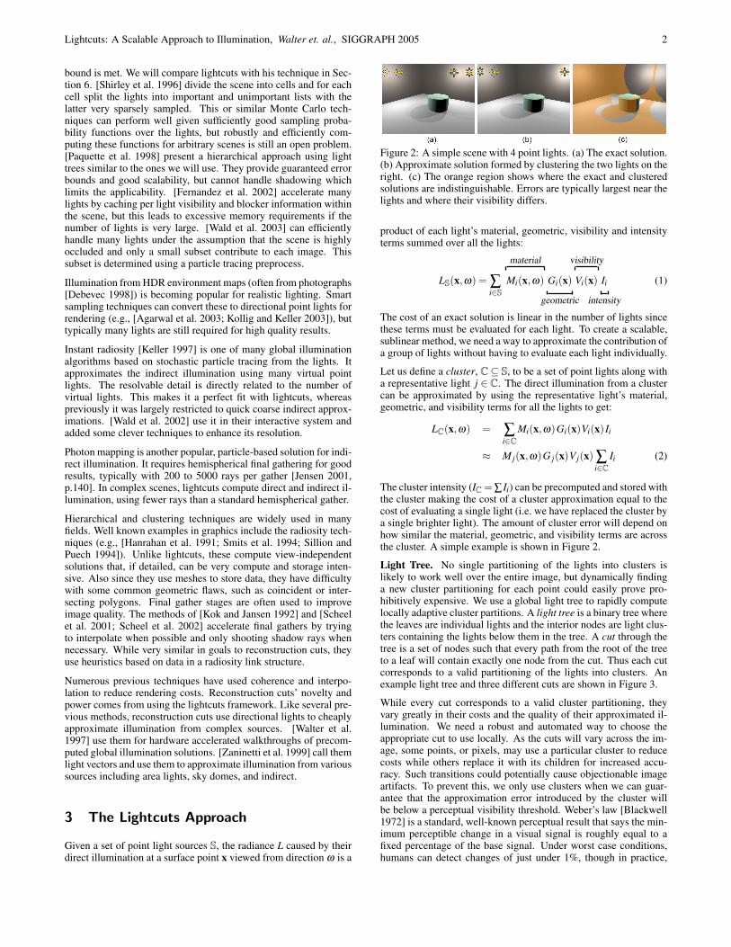
Figure 2: A simple scene with 4 point lights. (a) The exact solution.(b) Approximate solution formed by clustering the two lights on theright. (c) The orange region shows where the exact and clusteredsolutions are indistinguishable. Errors are typically largest near thelights and where their visibility differs.

product of each light’s material, geometric, visibility and intensityterms summed over all the lights:

LS(x,ω) = ∑i∈S

material

Mi(x,ω) Gi(x)

geometric

visibility

Vi(x) Ii

intensity

(1)

The cost of an exact solution is linear in the number of lights sincethese terms must be evaluated for each light. To create a scalable,sublinear method, we need a way to approximate the contribution ofa group of lights without having to evaluate each light individually.

Let us define a cluster, C⊆ S, to be a set of point lights along witha representative light j ∈ C. The direct illumination from a clustercan be approximated by using the representative light’s material,geometric, and visibility terms for all the lights to get:

LC(x,ω) = ∑i∈C

Mi(x,ω)Gi(x)Vi(x) Ii

≈ M j(x,ω)G j(x)V j(x) ∑i∈C

Ii (2)

The cluster intensity (IC = ∑ Ii) can be precomputed and stored withthe cluster making the cost of a cluster approximation equal to thecost of evaluating a single light (i.e. we have replaced the cluster bya single brighter light). The amount of cluster error will depend onhow similar the material, geometric, and visibility terms are acrossthe cluster. A simple example is shown in Figure 2.

Light Tree. No single partitioning of the lights into clusters islikely to work well over the entire image, but dynamically findinga new cluster partitioning for each point could easily prove pro-hibitively expensive. We use a global light tree to rapidly computelocally adaptive cluster partitions. A light tree is a binary tree wherethe leaves are individual lights and the interior nodes are light clus-ters containing the lights below them in the tree. A cut through thetree is a set of nodes such that every path from the root of the treeto a leaf will contain exactly one node from the cut. Thus each cutcorresponds to a valid partitioning of the lights into clusters. Anexample light tree and three different cuts are shown in Figure 3.

While every cut corresponds to a valid cluster partitioning, theyvary greatly in their costs and the quality of their approximated il-lumination. We need a robust and automated way to choose theappropriate cut to use locally. As the cuts will vary across the im-age, some points, or pixels, may use a particular cluster to reducecosts while others replace it with its children for increased accu-racy. Such transitions could potentially cause objectionable imageartifacts. To prevent this, we only use clusters when we can guar-antee that the approximation error introduced by the cluster willbe below a perceptual visibility threshold. Weber’s law [Blackwell1972] is a standard, well-known perceptual result that says the min-imum perceptible change in a visual signal is roughly equal to afixed percentage of the base signal. Under worst case conditions,humans can detect changes of just under 1%, though in practice,


#1 #2 #3 #4

1 2 3 4

1 4

4

1 2 3 4

1 4

4

1 2 3 4

1 4

4

1 2 3 4

1 4

4

1 1 1 1

2 2

4 Intensity

Light Tree

Clusters

IndividualLights

RepresentativeLight

Three Lightcuts

Figure 3: A light tree and three example cuts. The tree is shown onthe top with the representative lights and cluster intensities for eachnode. Leaves are individual lights while upper nodes are progres-sively larger light clusters. Each cut is a different partitioning of thelights into clusters (the orange cut is the same as Figure 2). Aboveeach cut, the regions where its error is small are highlighted.

the threshold is usually higher. In our experience, an error ratio of2% results in no visible artifacts across a wide variety of scenes andwas used for all our results. Changing this value can be used to varythe tradeoff between performance and accuracy.

Choosing Lightcuts. Using a relative error criterion requires anestimate of total radiance before we can decide whether a particularcluster is usable. To solve this difficulty, we start with a very coarsecut (e.g., the root of the light tree) and then progressively refine ituntil our error criterion is met. For each node in the cut we computeboth its cluster estimate (Equation 2) and an upper bound on itserror (Section 4.1). Each refinement step considers the node in thecurrent cut with the largest error bound. If its error bound is greaterthan our error ratio times the current total illumination estimate, weremove it from the cut, replace it with its two children from the lighttree, compute their cluster estimates and error bounds, and updateour estimate of the total radiance. Otherwise, the cut obeys ourerror criterion and we are done. We call such a cut, a lightcut.

To make this process more efficient, we require that the represen-tative light for a cluster be the same as for one of its two children.This allows us to reuse the representative light’s material, geomet-ric and visibility terms when computing that child. We use a heapdata structure to efficiently find the cluster node in the cut with thehighest error bound. If present in the cut, individual lights (i.e. lighttree leaf nodes) are computed exactly and thus have zero error.

Our relative error criterion overestimates the visibility of errors invery dark regions. For example, a fully occluded point would beallowed zero error, but even at black pixels sufficiently small errorsare not visible. Therefore, we also set a maximum cut size and, ifthe total number of nodes on the cut reaches this limit, stop furtherrefinement. We chose our maximum cut size of 1000 to be largeenough to rarely be reached in our results and then only in darkregions where the extra error is not visible.

4 Implementing Lightcuts

Our implementation supports three types of point lights: omni, ori-ented, and directional. Omni lights shine equally in all directions

from a single point. Oriented lights emit in a cosine-weighted hemi-spherical pattern defined by their orientation, or direction of max-imum emission. Directional lights simulate an infinitely far awaysource emitting in a single direction. All lights have an intensity Ii.

Building the Light Tree. The light tree groups point lights togetherinto clusters. Ideally, we want to maximize the quality of the clus-ters it creates (i.e. combine lights with the greatest similarity in theirmaterial, geometric and visibility terms). We approximate this bygrouping lights based on spatial proximity and similar orientation.

We divide the point lights by type into separate omni, oriented, anddirectional lists and build a tree for each. Conceptually though, wethink of them as part of a single larger tree. Each cluster records itstwo children, its representative light, its total intensity IC, an axis-aligned bounding box, and an orientation bounding cone. The coneis only needed for oriented lights. Although infinitely far away,directional lights are treated as points on the unit sphere when com-puting their bounding boxes. This allows directional lights to usethe same techniques as other point lights when building light treesand, more importantly, later for bounding their material terms Mi.

Similarity Metric. Each tree is built using a greedy, bottom-up ap-proach by progressively combining pairs of lights and/or clusters.At each step we choose the pair that will create the smallest clus-ter according to our cluster size metric IC(α2

C + c2 (1− cosβC)2),where αC is the diagonal length of the cluster bounding box and βCis the half-angle of its bounding cone. The constant c controls therelative scaling between spatial and directional similarity. It is setto the diagonal of the scene’s bounding box for oriented lights andzero for omni and directional lights.

The representative light for a cluster is always the same as for oneof its children and is chosen randomly based on the relative intensi-ties of the children. Each individual light is its own representative.Thus the probability of a light being the representative for a clusteris proportional to its intensity. This makes the cluster approxima-tion in Equation 2 unbiased in a Monte Carlo sense. However oncechosen, the same representative light is used for that cluster over theentire image. Tree building, by its very nature, cannot be sublinearin the number of lights, but is generally not a significant cost sinceit only has to be done once per image (or less if the lights are static).

4.1 Bounding Cluster Error

To use the lightcuts approach, we need to compute reasonablycheap and tight upper bounds on the cluster errors (i.e. the differ-ence between the exact and approximate versions of Equation 2).By computing upper bounds on the material, geometric, and vis-ibility terms for a cluster, we can multiply these bounds with thecluster intensity to get an upper bound for both the exact and ap-proximated cluster results. Since both are positive, this is also anupper bound on the cluster error (i.e. their absolute difference).

Visibility Term. The visibility of a point light is typically zeroor one but may be fractional (e.g., if semitransparent surfaces areallowed). Conservatively bounding visibility in arbitrary scenes isa hard problem, so we will use the trivial upper bound of one forthe visibility term (i.e. all lights are potentially visible).

Geometric Term. The geometric terms for our three point lighttypes are listed below, where yi is the light’s position and φi is theangle between an oriented light’s direction of maximum emissionand direction to the point x to be shaded.

Light Type Omni Oriented Directional

Gi(x) =1

‖yi−x‖2max(cosφi, 0)‖yi−x‖2 1

(3)


Bounding Volume for p

max(p )zMax cosθBoundz-axis

min(p )2x min(p )2

y+

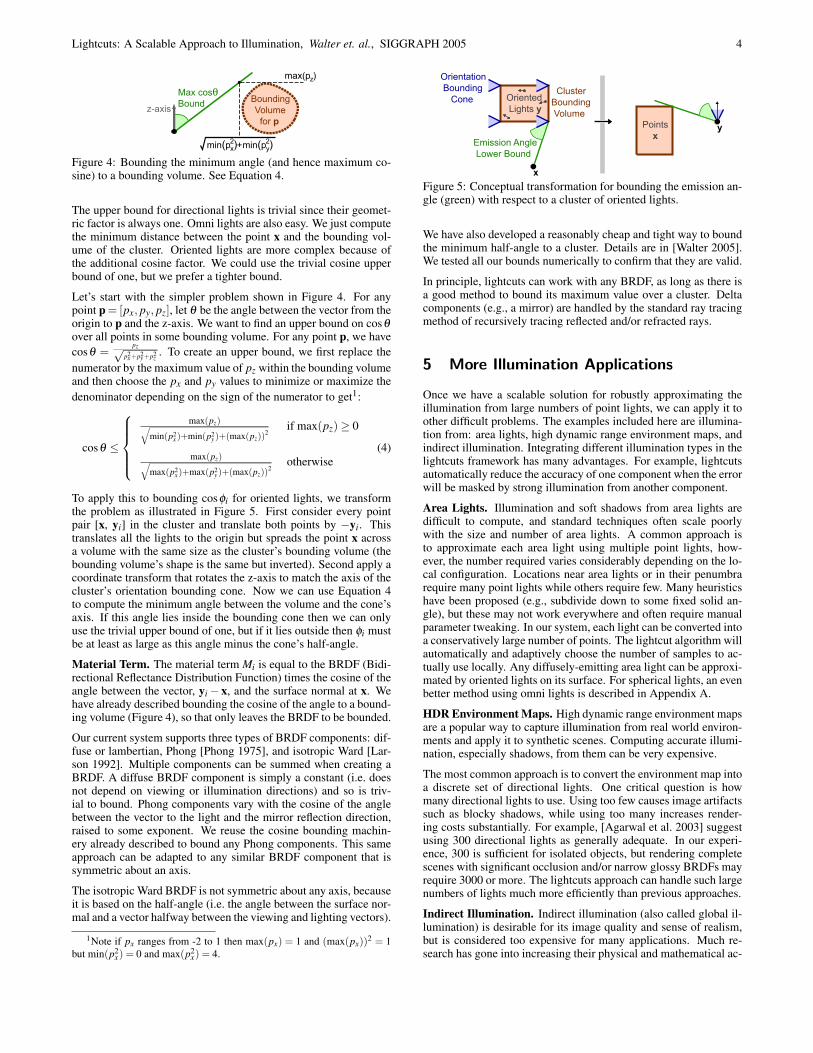
Figure 4: Bounding the minimum angle (and hence maximum co-sine) to a bounding volume. See Equation 4.

The upper bound for directional lights is trivial since their geomet-ric factor is always one. Omni lights are also easy. We just computethe minimum distance between the point x and the bounding vol-ume of the cluster. Oriented lights are more complex because ofthe additional cosine factor. We could use the trivial cosine upperbound of one, but we prefer a tighter bound.

Let’s start with the simpler problem shown in Figure 4. For anypoint p = [px, py, pz], let θ be the angle between the vector from theorigin to p and the z-axis. We want to find an upper bound on cosθ

over all points in some bounding volume. For any point p, we havecosθ =

pz√p2x +p2y +p2z

. To create an upper bound, we first replace thenumerator by the maximum value of pz within the bounding volumeand then choose the px and py values to minimize or maximize thedenominator depending on the sign of the numerator to get1:

cosθ ≤

max(pz)√

min(p2x)+min(p2

y)+(max(pz))2

if max(pz)≥ 0

max(pz)√max(p2

x)+max(p2y)+(max(pz))

2otherwise

(4)

To apply this to bounding cosφi for oriented lights, we transformthe problem as illustrated in Figure 5. First consider every pointpair [x, yi] in the cluster and translate both points by −yi. Thistranslates all the lights to the origin but spreads the point x acrossa volume with the same size as the cluster’s bounding volume (thebounding volume’s shape is the same but inverted). Second apply acoordinate transform that rotates the z-axis to match the axis of thecluster’s orientation bounding cone. Now we can use Equation 4to compute the minimum angle between the volume and the cone’saxis. If this angle lies inside the bounding cone then we can onlyuse the trivial upper bound of one, but if it lies outside then φi mustbe at least as large as this angle minus the cone’s half-angle.

Material Term. The material term Mi is equal to the BRDF (Bidi-rectional Reflectance Distribution Function) times the cosine of theangle between the vector, yi− x, and the surface normal at x. Wehave already described bounding the cosine of the angle to a bound-ing volume (Figure 4), so that only leaves the BRDF to be bounded.

Our current system supports three types of BRDF components: dif-fuse or lambertian, Phong [Phong 1975], and isotropic Ward [Lar-son 1992]. Multiple components can be summed when creating aBRDF. A diffuse BRDF component is simply a constant (i.e. doesnot depend on viewing or illumination directions) and so is triv-ial to bound. Phong components vary with the cosine of the anglebetween the vector to the light and the mirror reflection direction,raised to some exponent. We reuse the cosine bounding machin-ery already described to bound any Phong components. This sameapproach can be adapted to any similar BRDF component that issymmetric about an axis.

The isotropic Ward BRDF is not symmetric about any axis, becauseit is based on the half-angle (i.e. the angle between the surface nor-mal and a vector halfway between the viewing and lighting vectors).

1Note if px ranges from -2 to 1 then max(px) = 1 and (max(px))2 = 1but min(p2

x) = 0 and max(p2x) = 4.

Oriented Lights y

ClusterBounding Volume

Orientation Bounding Cone

Emission Angle Lower Bound

x

Points x

y

Figure 5: Conceptual transformation for bounding the emission an-gle (green) with respect to a cluster of oriented lights.

We have also developed a reasonably cheap and tight way to boundthe minimum half-angle to a cluster. Details are in [Walter 2005].We tested all our bounds numerically to confirm that they are valid.

In principle, lightcuts can work with any BRDF, as long as there isa good method to bound its maximum value over a cluster. Deltacomponents (e.g., a mirror) are handled by the standard ray tracingmethod of recursively tracing reflected and/or refracted rays.

5 More Illumination Applications

Once we have a scalable solution for robustly approximating theillumination from large numbers of point lights, we can apply it toother difficult problems. The examples included here are illumina-tion from: area lights, high dynamic range environment maps, andindirect illumination. Integrating different illumination types in thelightcuts framework has many advantages. For example, lightcutsautomatically reduce the accuracy of one component when the errorwill be masked by strong illumination from another component.

Area Lights. Illumination and soft shadows from area lights aredifficult to compute, and standard techniques often scale poorlywith the size and number of area lights. A common approach isto approximate each area light using multiple point lights, how-ever, the number required varies considerably depending on the lo-cal configuration. Locations near area lights or in their penumbrarequire many point lights while others require few. Many heuristicshave been proposed (e.g., subdivide down to some fixed solid an-gle), but these may not work everywhere and often require manualparameter tweaking. In our system, each light can be converted intoa conservatively large number of points. The lightcut algorithm willautomatically and adaptively choose the number of samples to ac-tually use locally. Any diffusely-emitting area light can be approxi-mated by oriented lights on its surface. For spherical lights, an evenbetter method using omni lights is described in Appendix A.

HDR Environment Maps. High dynamic range environment mapsare a popular way to capture illumination from real world environ-ments and apply it to synthetic scenes. Computing accurate illumi-nation, especially shadows, from them can be very expensive.

The most common approach is to convert the environment map intoa discrete set of directional lights. One critical question is howmany directional lights to use. Using too few causes image artifactssuch as blocky shadows, while using too many increases render-ing costs substantially. For example, [Agarwal et al. 2003] suggestusing 300 directional lights as generally adequate. In our experi-ence, 300 is sufficient for isolated objects, but rendering completescenes with significant occlusion and/or narrow glossy BRDFs mayrequire 3000 or more. The lightcuts approach can handle such largenumbers of lights much more efficiently than previous approaches.

Indirect Illumination. Indirect illumination (also called global il-lumination) is desirable for its image quality and sense of realism,but is considered too expensive for many applications. Much re-search has gone into increasing their physical and mathematical ac-


Lightcut Image Reference Image

Error Image 16 x Error Image

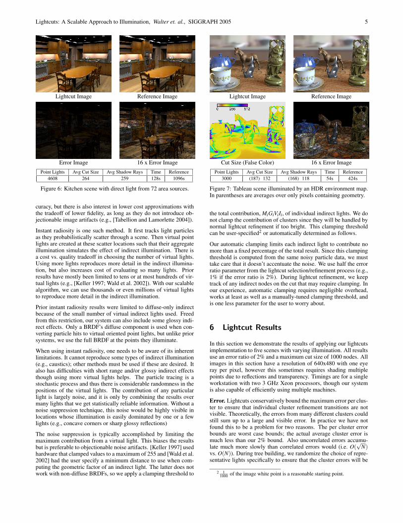
Point Lights Avg Cut Size Avg Shadow Rays Time Reference4608 264 259 128s 1096s

Figure 6: Kitchen scene with direct light from 72 area sources.

curacy, but there is also interest in lower cost approximations withthe tradeoff of lower fidelity, as long as they do not introduce ob-jectionable image artifacts (e.g., [Tabellion and Lamorlette 2004]).

Instant radiosity is one such method. It first tracks light particlesas they probabilistically scatter through a scene. Then virtual pointlights are created at these scatter locations such that their aggregateillumination simulates the effect of indirect illumination. There isa cost vs. quality tradeoff in choosing the number of virtual lights.Using more lights reproduces more detail in the indirect illumina-tion, but also increases cost of evaluating so many lights. Priorresults have mostly been limited to tens or at most hundreds of vir-tual lights (e.g., [Keller 1997; Wald et al. 2002]). With our scalablealgorithm, we can use thousands or even millions of virtual lightsto reproduce more detail in the indirect illumination.

Prior instant radiosity results were limited to diffuse-only indirectbecause of the small number of virtual indirect lights used. Freedfrom this restriction, our system can also include some glossy indi-rect effects. Only a BRDF’s diffuse component is used when con-verting particle hits to virtual oriented point lights, but unlike priorsystems, we use the full BRDF at the points they illuminate.

When using instant radiosity, one needs to be aware of its inherentlimitations. It cannot reproduce some types of indirect illumination(e.g., caustics); other methods must be used if these are desired. Italso has difficulties with short range and/or glossy indirect effectsthough using more virtual lights helps. The particle tracing is astochastic process and thus there is considerable randomness in thepositions of the virtual lights. The contribution of any particularlight is largely noise, and it is only by combining the results overmany lights that we get statistically reliable information. Without anoise suppression technique, this noise would be highly visible inlocations whose illumination is easily dominated by one or a fewlights (e.g., concave corners or sharp glossy reflections)

The noise suppression is typically accomplished by limiting themaximum contribution from a virtual light. This biases the resultsbut is preferable to objectionable noise artifacts. [Keller 1997] usedhardware that clamped values to a maximum of 255 and [Wald et al.2002] had the user specify a minimum distance to use when com-puting the geometric factor of an indirect light. The latter does notwork with non-diffuse BRDFs, so we apply a clamping threshold to

Lightcut Image Reference Image

Cut Size (False Color) 16 x Error Image

Point Lights Avg Cut Size Avg Shadow Rays Time Reference3000 (187) 132 (168) 118 54s 424s

Figure 7: Tableau scene illuminated by an HDR environment map.In parentheses are averages over only pixels containing geometry.

the total contribution, MiGiViIi, of individual indirect lights. We donot clamp the contribution of clusters since they will be handled bynormal lightcut refinement if too bright. This clamping thresholdcan be user-specified2 or automatically determined as follows.

Our automatic clamping limits each indirect light to contribute nomore than a fixed percentage of the total result. Since this clampingthreshold is computed from the same noisy particle data, we musttake care that it doesn’t accentuate the noise. We use half the errorratio parameter from the lightcut selection/refinement process (e.g.,1% if the error ratio is 2%). During lightcut refinement, we keeptrack of any indirect nodes on the cut that may require clamping. Inour experience, automatic clamping requires negligible overhead,works at least as well as a manually-tuned clamping threshold, andis one less parameter for the user to worry about.

6 Lightcut Results

In this section we demonstrate the results of applying our lightcutsimplementation to five scenes with varying illumination. All resultsuse an error ratio of 2% and a maximum cut size of 1000 nodes. Allimages in this section have a resolution of 640x480 with one eyeray per pixel, however this sometimes requires shading multiplepoints due to reflections and transparency. Timings are for a singleworkstation with two 3 GHz Xeon processors, though our systemis also capable of efficiently using multiple machines.

Error. Lightcuts conservatively bound the maximum error per clus-ter to ensure that individual cluster refinement transitions are notvisible. Theoretically, the errors from many different clusters couldstill sum up to a large and visible error. In practice we have notfound this to be a problem for two reasons. The per cluster errorbounds are worst case bounds; the actual average cluster error ismuch less than our 2% bound. Also uncorrelated errors accumu-late much more slowly than correlated errors would (i.e. O(

√N)

vs. O(N)). During tree building, we randomize the choice of repre-sentative lights specifically to ensure that the cluster errors will be

2 11000 of the image white point is a reasonable starting point.


Kitchen Tableau Grand Central TempleModel Polygons Number of Point Lights Per Pixel Averages Tree Image

Direct Env Map Indirect Total (d+e+i) Lightcut Size Shadow Rays Build TimeKitchen 388552 (72) 4608 5064 50000 59672 (54+244+345) 643 (0.8%) 478 3.4s 290sTableau 630843 0 3000 10000 13000 (0+112+104) 216 (1.1%) 145 0.9s 79sGrand Central 1468407 (820) 38400 5064 100000 143464 (73+136+480) 689 (0.33%) 475 9.7s 409sTemple 2124003 0 5064 500000 505064 (0+185+437) 622 (0.07%) 373 44s 225sBigscreen 628046 (4) 614528 0 25000 639528 (83+0+222) 305 (0.04%) 228 46s 98s

Figure 9: Lightcut results for 640x480 images of our five scenes with all illumination components enabled. Average cut sizes include howmany came from each of the three components: direct, environment map, and indirect. Average shadow rays per pixel is also shown as apercentage of the total number of lights. The aliasing (e.g., windows in Grand Central) is due to using only one eye ray per pixel here.

statistically uncorrelated. Essentially, lightcuts provide a stochas-tic error bound rather than an absolute one; large total errors arepossible but very unlikely.

The kitchen model, shown in Figure 6, is based on part of an ac-tual house. It contains 72 area sources, each approximated using 64point lights for a total of 4608 point lights. Even a close examina-tion reveals no visible differences between the lightcut result and areference image that evaluated each point light exactly. The errorimage appears nearly black. Magnifying the errors by a factor 16shows that, as expected, the errors are generally larger in brighterregions and consist of many discontinuities caused by transitionsbetween using a cluster and refining it. The lightcut image took128 seconds with an average cut size of 264 and 259 shadow raysper pixel, while the reference image took much longer at 1096 sec-onds with an average of 3198 shadow rays per pixel. Shadow raysare not shot to lights whose material or geometric terms are zero.

The tableau model, in Figure 7, has several objects with differentglossy materials on a wooden tray and lit by a captured HDR envi-ronment map (the Kitchen map from [Debevec 1998], not related toour kitchen model). We used the technique of [Agarwal et al. 2003]to convert this map to 3000 directional lights for rendering. Againthere are no visible differences between the reference image and thelightcut image. A visualization shows the per pixel cut size (i.e. thenumber of nodes on the lightcut). Cut size corresponds closely torendering cost and tends to be largest in regions of high occlusion.

Scalability. As the number of point lights increases, lightcuts scalefundamentally better (i.e. sublinearly vs. linearly) than prior tech-niques. To demonstrate this, we varied the number of point lightsin the kitchen and tableau examples above by changing the numberof point lights created per area light and directional lights created

Tableau with HDR Environment Map

0

100

200

300

400

500

600

0 1000 2000 3000 4000Number of Directional Lights

Tim

e (s

ecs)

NaiveWardLightcut

Kitchen with Area Lights

0

100

200

300

400

500

600

0 1000 2000 3000 4000 5000Number of Point Lights

Tim

e (s

ecs)

NaiveWardLightcut

Figure 8: Lightcut performance scales fundamentally better (i.e.sublinearly) as the number of point lights increase.

from the environment map, respectively. Image times vs. numberof point lights are shown in Figure 8 for both lightcuts and the naive(reference) solutions. We also compare to [Ward 1994] which weconsider the best of the alternative approaches with respect to gen-erality, robustness, and the ability to handle thousands of lights.

Ward’s technique computes the potential contribution of all thelights assuming full visibility, sorts these in decreasing order, andthen progressively evaluates their visibility until the total remain-ing potential contribution falls below a fraction of the total of theevaluated lights (10% in our comparison). Since shadow rays(i.e.visibility tests) are usually the dominant cost, reducing themusually more than compensates for the cost of the sort (true for thekitchen and just barely for tableau). However, the cost still behaveslinearly as shown in plots. Suppose we had 1000 lights whose un-occluded contributions would be roughly equal. We would have tocheck the visibility of at least 800 lights to meet a 10% total errorbound3, and this number grows linearly with the lights. This caseis the Achilles’ heel of Ward’s technique, or any technique that pro-vides an absolute error bound. Lightcuts superior scalability meansthat its advantage grows rapidly as the number of lights increase.

Mixed Illumination. We can use this scalability to compute richerand more complex lighting in our scenes as shown in Figure 9.Grand Central is a model of the famous landmark in New YorkCity and contains 220 omni point lights distributed near the ceil-ing of the main hall and 600 spherical lights in chandeliers in theside hallways. The real building actually contains even more lights.Temple is a model of an Egyptian temple and is our most geometri-cally complex at 2.1 million triangles. Such geometric complexity

3Using the optimal value of 0.5 for the visibility of the untested lights.

Bigscreen Model Cut Size (False Color)

Figure 10: Bigscreen model. See Figure 9 for statistics.


causes aliasing problems because we are using only one eye rayper pixel. The next section will introduce reconstruction cuts thatallow us to perform anti-aliasing at a reduced cost. The bigscreenmodel (Figure 10) shows an office lit by two overhead area lights(64 points each) and by two large HDR monitors displaying imagesof our other scenes. The monitors have a resolution of 640x480 andwere simulated by converting each of their pixels into a point light.

We’ve added a sun/sky model from [Preetham et al. 1999], whichacts like an HDR environment map, to the kitchen, Grand Cen-tral, and temple. The sun is converted into 64 directional lightsand the sky into 5000 directional lights distributed, uniformly overthe sphere of directions. We also added indirect illumination to allthe models using the instant radiosity approach. In the kitchen andGrand Central models only a fraction of particles from the sun/skymake it through the windows into the interior; many indirect lightsend up on the outside of the buildings. With our scalable algorithm,we can compensate by generating more indirect lights. Temple usesthe most indirect lights because its model covers the largest area.

With lightcuts the number of lights is not strongly correlated withimage cost. Instead the strongest predictor of image cost is thedegree of occlusion of the light sources. Thus the kitchen and par-ticularly Grand Central are the most expensive because of the highdegree of occlusion to their light sources especially the sun/sky. Al-though temple and bigscreen have more point lights and geometry,they are less expensive due to their higher visibility.

Shadow rays are the dominant cost in lightcuts and consumeroughly 50% of the total time, even though this is the most opti-mized part of our code (written in C while the rest is Java). Com-puting error bounds consumes another 20% and 10% is shading.Various smaller operations including tree traversal, maintaining themax heap, updating estimates, etc. consume the rest. Tree buildingstarts to be significant for the largest numbers of lights but there aremuch faster methods than our simple greedy approach.

Bound Tightness. The ability to cheaply bound the maximum con-tribution, and hence the error, from a cluster is essential for our scal-ability. Using tighter (and probably more expensive) bounds mightreduce the average cut size and potentially reduce overall costs. InFigure 11, we show the cut sizes that would result if we had exactbounds on the product of the geometric and material terms Gi Mi.This is the best we can hope to achieve without bounds on visibility.Overall, our bounds perform very well. Indirect lights are harder tobound due to their wider dispersal, but our bounds still performwell. Significant further gains will likely require efficient conserva-tive visibility bounds. This is possible in many specific cases (e.g.,see [Cohen-Or et al. 2003]), but an unsolved problem in general.

Model Illumination Point Avg Cut SizeLights Lightcut Exact Gi Mi Bound

Kitchen Direct 4608 264 261+ Indirect 54608 643 497

Tableau Env Map 3000 132 120+ Indirect 13000 216 153

Temple Sun/Sky 5064 294 287

Figure 11: How tighter bounds would affect lightcut size.

7 Reconstruction Cuts

Reconstruction cuts are a new technique for exploiting spatial co-herence to reduce average shading costs. The idea is to computelightcuts sparsely over the image (e.g., at the corners of imageblocks) and then appropriately interpolate their illumination infor-mation to shade the rest of the image. Although lightcuts allow

the scalable computation of accurate illumination from thousandsor millions of point lights, they still typically require shooting hun-dreds of shadow rays per shaded point. By taking a slightly lessconservative approach, reconstruction cuts are able to exploit illu-mination smoothness to greatly reduce the shading cost.

The simplest approach would be to simply interpolate the radiancesfrom the sparse lightcuts (e.g., Gouraud shading), but this wouldcause objectionable blurring of high frequency image features suchas shadow boundaries and glossy highlights. Many extensions ofthis basic idea have been proposed to preserve particular types offeatures (e.g., [Ward and Heckbert 1992] interpolates irradiance topreserve diffuse textures and [Krivanek et al. 2005] use multipledirectional coefficients to preserve low frequency gloss), but wewant to preserve all features including sharp shadow boundaries.

To compute a reconstruction cut at a point, we first need a set ofnearby samples (i.e. locations where lightcuts have been computedand processed for easy interpolation). Then we perform a top-downtraversal of the global light tree. If all the samples agree that a nodeis occluded then we immediately discard it. If a node’s illuminationis very similar across the samples then we cheaply interpolate it us-ing impostor lights. These are special directional lights designed tomimic the aggregate behavior of a cluster as recorded in the sam-ples. Otherwise we default to lightcut-style behavior; refining downthe tree until the errors will be small enough and using the clusterapproximation from Equation 2, including shooting shadow rays.

Interpolating or discarding nodes, especially if high up in the tree,provides great cost savings. However when the samples straddle ashadow boundary or other sharp feature, we revert to more robustbut expensive methods for the affected nodes. Because reconstruc-tion cuts effectively include visibility culling, they are less affectedby high occlusion scenes than lightcuts are.

Samples. A sample k is created by first computing a lightcut for apoint xk and viewing direction ωk. This will include computing aradiance estimate Lk

n at every light tree node n on the lightcut usingEquation 2. For each node above the cut, we define Lk

n as the sum ofthe radiance estimates of all of its descendants on the cut. Similarly,the total radiance estimate Lk

T is the sum over all nodes in the cut.

To convert a lightcut into a sample, we create impostor directionalpoint lights (with direction dk

n and intensity γkn ) for each node on

or above the cut. Their direction mimics the average direction ofincident light from the corresponding cluster or light, and their illu-mination exactly reproduces the radiance estimate Lk

n at the samplepoint. Impostor lights are never occluded and hence relatively inex-pensive to use (i.e. both visibility and geometric terms equal one).

For nodes on the cut, the impostor direction dkn is the same as from

its representative light. For nodes above the cut, dkn is the average

of the directions for its descendants on the cut, weighted by theirrespective radiance estimates. Using this direction we can evaluatethe impostor’s material term Mk

n and its intensity γkn . We also com-

pute a second intensity Γkn based on the total radiance estimate and

used to compute relative thresholds (i.e. relative magnitude of thenode compared to the total illumination).

γkn = Lk

n(xk,ωk) / Mk

n(xk,ωk) (5)

Γkn = Lk

T(xk,ωk) / Mkn(xk,ωk) (6)

Occasionally we need an impostor directional light for a node belowa sample’s lightcut. These are created as needed and use the samedirection as their ancestor on the cut, but with impostor’s intensitydiminished by the ratio between the node’s cluster intensity IC andthat of its ancestor.


Exact sample size depends on the lightcut, but 24KB is typical.Samples store 32 bytes per node on or above the lightcut whichincludes 7 floats (1 for Γk

n and 3 each for dkn and γk

n ) and an offset toits children’s data if present. We decompose the image into blocksso that only a small subset of the samples is kept at any time.

Computing a Reconstruction Cut. Given a set of samples, wewant to use them to quickly estimate Equation 1. Reconstructioncuts use a top-down traversal of the global light tree. At each nodevisited, we compute the minimum and maximum impostor inten-sities γk

n over the samples k, and a threshold τn, the lightcut errorratio (e.g.,2%) times the minimum of Γk

n over the samples. Thenwe select the first applicable rule from:

1. Discard. If max(γkn) = 0, then the node had zero radiance at all

the samples and is assumed to have zero radiance here as well.

2. Interpolate. If max(γkn)−min(γk

n) < τn and min(γkn) > 0, then

we compute weighted averages of dkn and γk

n to create an inter-polated impostor directional light. The estimate for this nodeis then equal to the material term for the interpolated directiontimes the interpolated intensity.

3. Cluster Evaluate. If max(γkn) < τn or if we are at a leaf node

(i.e. individual light), then we estimate the radiance using Equa-tion 2. This includes shooting a shadow ray to the representa-tive light if the material and geometric terms are not zero.

4. Refine. Otherwise we recurse down the tree and perform thesame tests on each of this node’s two children.

While the above rules cover most cases, a few refinements areneeded to prevent occasional artifacts (e.g., on glossy materials).First, we disallow interpolation inside glossy highlights. The max-imum possible value for a diffuse BRDF is 1/π . When computingthe material term for an interpolated impostor, if its BRDF value isgreater than 1/π , then the direction must lie inside the gloss lobeof a material and we disallow interpolation for that node. Second,cluster evaluation is only allowed for nodes that are at, or below, atleast one of the sample lightcuts. Nodes below all the sample light-cuts do not use interpolation, since they have no good informationto interpolate. Third, if the result of a cluster evaluation is muchlarger than expected, we recursively evaluate its children instead.

Image Blocks. The image is first divided into 16x16 pixel blockswhich do not share sample information. This keeps storage require-ments low and allows easy parallel processing. To process eachblock, we initially divide it into 4x4 pixel blocks but may divide itfurther based on the following tests.

To compute a block, we compute samples at its corners, shoot eyerays through its pixels, and test to see if the resulting points matchthe corner samples. If using anti-aliasing, there will be multipleeye rays per pixel. A set of eye rays is said to match if they all hitsurfaces with the same type of material and with surface normalsthat differ by no more than some angle (e.g., 30 degrees). We alsouse a cone test to detect possible local shadowing conditions thatrequire block subdivision (e.g., see Figure 12). For each eye ray,we construct a cone starting at its intersection point and centeredaround the local surface normal. If the intersection point for anyother eye ray lies within this cone, then the block fails the conetest. The cone test uses true geometric normals and is unaffectedby shading effects such as bump maps or interpolated normals.

If the eye rays do not match and the block is bigger than a pixel,then we split the block into four smaller blocks and try again. Ifthe block is pixel-sized, we relax the requirements, omit the conetest, and only require that each eye ray match at least two nearbysamples. If there are still not enough matching samples, then wecompute a new sample at that eye ray.

Cones

Surface Normals

Passes FailsFigure 12: Block cone test. (Right) fails because the upper twopoints lie within the cone of the lower point. (Left) passes becauseno points lie within the cones defined by the other points.

After block subdivision we compute a color for each remaining eyeray using reconstruction cuts. For blocks larger than a pixel we usethe four corners as the set of nearby samples and use image-spacebilinear interpolation weights when interpolating impostors. Eyerays within pixel-sized blocks use their set of matching samplesand interpolation weights proportional to the world-space inversedistance squared between the surface point and the sample points.

8 Reconstruction Cut Results

In this section we present some results of applying the reconstruc-tion cuts technique to our scenes. Result images and statisticsare shown in Figure 13. These results are adaptively anti-aliased[Painter and Sloan 1989] using between 5 and 50 eye rays per pixel.The sparse samples are computed using lightcuts with the same pa-rameters as in Section 6. Most of the shading is done using recon-struction cuts that interpolate intelligently between the samples.

By exploiting spatial coherence, reconstruction cuts can shadepoints using far fewer shadow rays than lightcuts. While a lightcutrequires a few hundred shadow rays, on average a reconstruction cutuses less than fourteen in our results. In fact, most of our shadowrays are used for computing the sparse samples (lightcuts) eventhough there are 15-25 times more reconstruction cuts. This al-lows us to generate much higher quality images, with anti-aliasing,at a much lower cost than with lightcuts alone. For the same sizeimages, the results are both higher quality and have similar or lowercost than those in Section 6. Moreover for larger images, renderingcost increases more slowly than the number of pixels.

Samples are computed at the corners of adaptively sized imageblocks (between 4x4 and 1x1 pixels in size) and occasionally withina pixel when needed (shown as 1x1+ in red). As shown for the tem-ple image, most of the pixels in all images lie within 4x4 blocks.An average of less than one sample per pixel is needed even withanti-aliasing requiring multiple eye rays per pixel. We could al-low larger blocks (e.g., 8x8) but making the samples even sparserwhere they are already sparse has less benefit and can be counter-productive because reconstruction cut cost is strongly related to thesimilarity of the nearby samples.

Because the accuracy of reconstruction cuts relies on having nearbysamples that span the local lighting conditions, there is a possibil-ity of missing small features in between samples. While this doeshappen occasionally, it is rarely problematic. For example in a fewplaces, the interpolation smooths over the grooves in the pillars ofthe temple, but the errors are quite small and we have found thatpeople have great difficulty in noticing them. Future improvementsin the block refinement rules could fix these errors.

A Metropolis solution and its magnified (5x) differences with ourresult are shown in Figure 14. Metropolis [Veach and Guibas 1997]is considered the best and fastest of the general purpose MonteCarlo solvers. Its result took 13 times longer to compute than oursand still contains some visible noise. The main differences are thenoise in the Metropolis solution and some corner darkening in our


Kitchen Tableau Temple (Reconstruction Block Size)

Grand Central Temple

Model Point Per Pixel Averages Avg Shadow Rays Per Pixel Avg Per Reconstruction Cut Image TimeLights Eye Rays Samples Samples Recon Cuts Shadow Rays Interpolations 1280x960 640x480

Kitchen 59672 5.4 0.29 143 50 9.1 14.4 672s 257sTableau 13000 5.4 0.23 50 41 10.6 17.8 298s 111sGrand Central 143464 6.9 0.46 225 93 13.3 11.5 1177s 454sTemple 505064 5.5 0.25 91 52 9.4 6.0 511s 189sBigscreen 639528 5.3 0.25 64 24 4.6 15.0 260s 98s

Figure 13: Reconstruction cut results for 1280x960 images (except where noted) of our scenes. Images are anti-aliased using 5 to 50 eyerays per pixel adaptively. Samples (lightcuts from Figure 9) are computed sparsely and most shading is computed using reconstruction cutsto interpolate intelligently. Reconstruction cuts are much less expensive and require many fewer shadow rays than lightcuts. Bigscreen imageis shown in Figure 1.

result. The latter is due to instant radiosity not reproducing veryshort range indirect illumination effects.

9 Conclusion

We have presented lightcuts as a new scalable unifying frameworkfor illumination. The core component is a strongly sublinear al-gorithm for computing the illumination from thousands or millionsof point lights using a perceptual error metric and conservative percluster error bounds. We have shown that it can greatly reduce thenumber of shadow rays, and hence cost, needed to compute illumi-nation from a variety of sources including area lights, HDR environ-ment maps, sun/sky models, and indirect illumination. Moreover itcan handle very complex scenes with detailed geometry and glossymaterials. We have also presented reconstruction cuts that furtherspeed shading by exploiting coherence in the illumination.

There are many ways in which this work can be improved and ex-

Metropolis Solution 5 x DifferenceFigure 14: Comparison with metropolis image for temple.

tended. For example, extending to additional illumination types(e.g., indirect components not handled by instant radiosity), inte-grating more types of light sources including non-diffuse sourcesand spot lights, developing bounds for more BRDF types, moreformal analysis of lightcuts stochastic error, further refinement ofthe reconstruction cut rules to exploit more coherence, and addingconservative visibility bounds to further accelerate lightcuts.


Acknowledgments

Many thanks to the modelers: Jeremiah Fairbanks (kitchen), Will Stokes(bigscreen), Moreno Piccolotto, Yasemin Kologlu, Anne Briggs, Dana Get-man (Grand Central) and Veronica Sundstedt, Patrick Ledda, and the Graph-ics Group at University of Bristol (temple). This work was supported byNSF grant ACI-0205438 and Intel Corporation. The views expressed in thisarticle are those of the authors and do not reflect the official policy or po-sition of the United States Air Force, Department of Defense, or the U. S.Government.

References

AGARWAL, S., RAMAMOORTHI, R., BELONGIE, S., AND JENSEN, H. W.2003. Structured importance sampling of environment maps. ACMTransactions on Graphics 22, 3 (July), 605–612.

BLACKWELL, H. R. 1972. Luminance difference thresholds. In Hand-book of Sensory Physiology, vol. VII/4: Visual Psychophysics. Springer-Verlag, 78–101.

COHEN-OR, D., CHRYSANTHOU, Y. L., SILVA, C. T., AND DURAND,F. 2003. A survey of visibility for walkthrough applications. IEEETransactions on Visualization and Computer Graphics 9, 3, 412–431.

DEBEVEC, P. 1998. Rendering synthetic objects into real scenes: Bridgingtraditional and image-based graphics with global illumination and highdynamic range photography. In Proceedings of SIGGRAPH 98, Com-puter Graphics Proceedings, Annual Conference Series, 189–198.

FERNANDEZ, S., BALA, K., AND GREENBERG, D. P. 2002. Local il-lumination environments for direct lighting acceleration. In RenderingTechniques 2002: 13th Eurographics Workshop on Rendering, 7–14.

HANRAHAN, P., SALZMAN, D., AND AUPPERLE, L. 1991. A rapid hi-erarchical radiosity algorithm. In Computer Graphics (Proceedings ofSIGGRAPH 91), vol. 25, 197–206.

HASENFRATZ, J.-M., LAPIERRE, M., HOLZSCHUCH, N., AND SILLION,F. 2003. A survey of real-time soft shadows algorithms. In Eurographics,Eurographics, Eurographics. State-of-the-Art Report.

JENSEN, H. W. 2001. Realistic image synthesis using photon mapping. A.K. Peters, Ltd.

KELLER, A. 1997. Instant radiosity. In Proceedings of SIGGRAPH 97,Computer Graphics Proceedings, Annual Conference Series, 49–56.

KOK, A. J. F., AND JANSEN, F. W. 1992. Adaptive sampling of arealight sources in ray tracing including diffuse interreflection. ComputerGraphics Forum (Eurographics ’92) 11, 3 (Sept.), 289–298.

KOLLIG, T., AND KELLER, A. 2003. Efficient illumination by high dy-namic range images. In Eurographics Symposium on Rendering: 14thEurographics Workshop on Rendering, 45–51.

KRIVANEK, J., GAUTRON, P., PATTANAIK, S., AND BOUATOUCH, K.2005. Radiance caching for efficient global illumination computation.IEEE Transactions on Visualization and Computer Graphics.

LARSON, G. J. W. 1992. Measuring and modeling anisotropic reflection. InComputer Graphics (Proceedings of SIGGRAPH 92), vol. 26, 265–272.

PAINTER, J., AND SLOAN, K. 1989. Antialiased ray tracing by adap-tive progressive refinement. In Computer Graphics (Proceedings of SIG-GRAPH 89), vol. 23, 281–288.

PAQUETTE, E., POULIN, P., AND DRETTAKIS, G. 1998. A light hierarchyfor fast rendering of scenes with many lights. Computer Graphics Forum17, 3, 63–74.

PHONG, B. T. 1975. Illumination for computer generated pictures. Com-mun. ACM 18, 6, 311–317.

PREETHAM, A. J., SHIRLEY, P. S., AND SMITS, B. E. 1999. A practicalanalytic model for daylight. In Proceedings of SIGGRAPH 99, ComputerGraphics Proceedings, Annual Conference Series, 91–100.

SCHEEL, A., STAMMINGER, M., AND SEIDEL, H.-P. 2001. Thrifty finalgather for radiosity. In Rendering Techniques 2001: 12th EurographicsWorkshop on Rendering, 1–12.

SCHEEL, A., STAMMINGER, M., AND SEIDEL, H. 2002. Grid based finalgather for radiosity on complex clustered scenes. Computer GraphicsForum 21, 3, 547–556.

SHIRLEY, P., WANG, C., AND ZIMMERMAN, K. 1996. Monte carlo tech-niques for direct lighting calculations. ACM Transactions on Graphics15, 1 (Jan.), 1–36.

SILLION, F. X., AND PUECH, C. 1994. Radiosity and Global Illumination.Morgan Kaufmann Publishers Inc.

SMITS, B., ARVO, J., AND GREENBERG, D. 1994. A clustering algorithmfor radiosity in complex environments. In Proceedings of SIGGRAPH94, Annual Conference Series, 435–442.

TABELLION, E., AND LAMORLETTE, A. 2004. An approximate globalillumination system for computer generated films. ACM Transactions onGraphics 23, 3 (Aug.), 469–476.

VEACH, E., AND GUIBAS, L. J. 1997. Metropolis light transport. InProceedings of SIGGRAPH 97, Computer Graphics Proceedings, AnnualConference Series, 65–76.

WALD, I., KOLLIG, T., BENTHIN, C., KELLER, A., AND SLUSALLEK, P.2002. Interactive global illumination using fast ray tracing. In RenderingTechniques 2002: 13th Eurographics Workshop on Rendering, 15–24.

WALD, I., BENTHIN, C., AND SLUSALLEK, P. 2003. Interactive globalillumination in complex and highly occluded environments. In Euro-graphics Symposium on Rendering: 14th Eurographics Workshop onRendering, 74–81.

WALTER, B., ALPPAY, G., LAFORTUNE, E. P. F., FERNANDEZ, S., ANDGREENBERG, D. P. 1997. Fitting virtual lights for non-diffuse walk-throughs. In Proceedings of SIGGRAPH 97, Computer Graphics Pro-ceedings, Annual Conference Series, 45–48.

WALTER, B. 2005. Notes on the Ward BRDF. Technical Report PCG-05-06, Cornell Program of Computer Graphics, Apr.

WARD, G. J., AND HECKBERT, P. 1992. Irradiance gradients. In ThirdEurographics Workshop on Rendering, 85–98.

WARD, G. 1994. Adaptive shadow testing for ray tracing. In Photorealis-tic Rendering in Computer Graphics (Proceedings of the Second Euro-graphics Workshop on Rendering), Springer-Verlag, New York, 11–20.

WOO, A., POULIN, P., AND FOURNIER, A. 1990. A survey of shadowalgorithms. IEEE Computer Graphics and Applications 10, 6 (Nov.),13–32.

ZANINETTI, J., BOY, P., AND PEROCHE, B. 1999. An adaptive methodfor area light sources and daylight in ray tracing. Computer GraphicsForum 18, 3 (Sept.), 139–150.

A Spherical LightsAny diffuse area light can be simulated using oriented lights on its surface.For spherical lights, we have developed a better technique that simulatesthem using omni lights (which are a better match for far field emission).Placing omni lights on the surface of the sphere would incorrectly make itappear too bright near its silhouette as compared to its center. Similarlya uniform distribution inside the volume of the sphere would exhibit thereverse problem. However, by choosing the right volume distribution insidethe sphere, we can correctly match the emission of a spherical light.

d(x) =1

π2R2√

R2− r2(x)(7)

The normalized point distribution d(x) is defined inside a sphere of radiusR where r2(x) is the squared distance from the sphere’s center. The beautyof this distribution is that it projects to a uniform distribution across theapparent solid angle of the sphere when viewed from any position outsidethe sphere, which is exactly the property we need. We also need a way togenerate random points according to this distribution. Given three uniformlydistributed random numbers, ξ1,ξ2,ξ3, in the range [0,1] we can computepoints with the right distribution for a sphere centered at the origin using:

x = R√

ξ1 cos(2πξ2)

y = R√

ξ1 sin(2πξ2)

z =√

R2− x2− y2 sin(π(ξ3−1/2))

(8)

The omni lights generated from spherical lights behave exactly like normalomni lights except that when computing their visibility factors, they canonly be occluded by geometry outside the sphere (i.e. their shadow raysterminate at the surface of the sphere).

lightcuts: a scalable approach to illuminationbjw/lightcuts.pdflightcuts: a scalable approach to...

Documents