Like Father, Like Son? Intergenerational Education Mobility in India∗

Mehtabul Azam 1

World Bank & IZA

Vipul Bhatt2

James Madison University

Abstract

This paper employs a novel strategy to create a unique, nationally representative father-son matched data for India and documents the extent of intergenerational mobility ineducational attainment. We provide an estimate of how India ranks among othernations, and study the evolution of intergenerational education mobility. For the birthcohorts from 1940-85, we find a declining cohort trend in the intergenerational elasticity(IGE) of educational attainment in India, at the aggregate level, for major castes, andstates. Finally, we find a positive correlation between a state’s ranking in per capitapublic education spending, and the IGE-based mobility measure.

JEL Codes: J6, I28

Keywords: Intergenerational Mobility, Educational Persistence, India

∗The findings, interpretations, and conclusions expressed in this paper are entirely those of the authors.They do not necessarily represent the views of the International Bank for Reconstruction and Develop-ment/World Bank and its affiliated organizations, or those of the Executive Directors of the World Bank orthe governments they represent.

1Azam: Consultant, World Bank, 1818 H ST, NW, Mail Stop: H11-1101 Washington, DC 20433.Email:mazam1@woldbank.org.

2Bhatt: Assistant Professor, James Madison University, Department of Economics, 421 Bluestone Drive,ZSH 433, Harrisonburg, VA-22807. Email:bhattvx@jmu.edu.

1

1. Introduction

In a recent opinion poll conducted in the U.S. a significant majority of the respondents

indicated that equality of opportunity is more important than equality of outcomes.3 In-

tergenerational persistence in economic status is an important mechanism in perpetuating

inequality of opportunities in a society. For instance, such persistence may differ across

groups of people in a society typically identified by race, gender, and region implying dif-

ferential access to opportunities for different groups. Hence, the extent to which economic

status is transmitted from one generation to the next has long been of interest to social

scientists and policy makers.

India serves as an excellent case study for intergenerational mobility for two reasons.

First, historically Indian society has been characterized by a high degree of social strati-

fication governed by the caste system wherein lower castes were typically associated with

poor economic outcomes. Although, the caste system has been weakened as a response to

various policy measures taken by the government of India, social identity still remains an

important dimension of social exclusion. Hence, gauging how such inertia in economic mo-

bility has changed over time is of interest. Second, although India has experienced rapid

economic growth in recent decades, this economic growth has been far from uniformly dis-

tributed on regional dimensions. Many large states have experienced below national average

economic growth and also have significant differences in terms access to education opportu-

nities (Chaudhuri and Ravallion, 2006; Emran and Shilpi, 2012; Asadullah and Yalonetzky,

2012).

Although, as argued above, understanding the extent of intergenerational mobility is

especially important for India, this issue has received relatively less attention mainly because

lack of suitable data for such kind of studies. Most of the existing studies rely on the co-

residence condition to identify father-son pairs from cross-sectional data (Jalan and Murgai,

3In an opinion poll on Economic Mobility and the American Dream, Pew Charitable Trust March 2009,when asked whether it was “more important to reduce inequality in America or to ensure everyone has afair chance of improving their economic standing”, 71 percent favored ensuring everyone had a fair chancecompared with 21 percent who thought it was more important to reduce inequality (Breen, 2010).

2

2008; Maitra and Sharma, 2009; Hnatkovskay et al., 2012; Emran and Shilpi, 2012) . This

leads to a significant loss of observations and more importantly raises serious sample selection

issue as coresident households may differ systematically from other households. For instance,

the identification of parental information achieved through co-residence, will either lead to

restricting the analysis to the young adults (Jalan and Murgai, 2008) or a cross -sectional

estimate based on a sample that is not representative of the adult population (Hnatkovskay

et al., 2012).4’5 In this paper we address this issue by creating a unique father-son matched

data, using the nationally representative India Human Development Survey, 2005 (IHDS),

that is not limited to coresident households. We believe that our data is more appropriate for

studying intergenerational mobility as it is representative of the entire adult male population

in India.

In any intergenerational study, the measurement of economic status remains an impor-

tant issue, and several studies proxy economic status by labor market characteristics such

as earnings, occupation, and educational attainment. In this paper, we focus on intergen-

erational mobility in educational attainment. Specifically, we estimate the intergenerational

elasticity (henceforth, IGE) of educational attainment as a measure of persistence (lack of

mobility) across generations. Although education is not the only proxy for economic status,

there are several advantages in using education instead of earnings to measure intergener-

ational mobility, especially in a developing country context where existence of long panel

data is rare. First, on the measurement side, education is less prone to serious errors than

earnings. Second, since most individuals complete their education by early or mid twenties,

life cycle biases are unlikely to bias estimation when compared with earnings. Finally, there

is a vast literature that shows that higher education is associated with higher earnings, better

health, and other economic outcomes (see Black and Devereux, 2011), rendering a measure

of intergenerational mobility based on education a reasonable proxy for mobility in overall

4Such limitations are expected if one uses data only for coresident parents to estimate intergenerationalmobility because such a condition is more likely to be satisfied for young adults. As a result the estimatesof intergenerational elasticities can be severely biased downwards (Franscesconi and Nicoletti, 2006).

5In Section 3.1 we discuss, in detail, the issue of co-residence in existing studies on India, the resultingdecline in the sample size, and the sample selection issue that can arise due to the use of co-residence formatching children with parents.

3

economic status.

This paper attempts to address three important issues in the context of India. First,

what is the extent of intergenerational mobility in educational attainment in India? Second,

how this mobility has evolved over time at the aggregate level? Third, do we observe a social

and a regional dimension in the evolution of intergenerational education mobility in India?

To shed light on this issue, we investigate the cohort trend in IGE by major castes, and by

major states.

The paper contributes to the existing literature in following ways. First, we are able to

match about 97% of the males aged 20-65 in our sample with their father information. As

a result, unlike other studies on India, the estimates presented in this paper do not suffer

from sample selection bias caused by limiting the analysis to adults coresiding with their

parents (see Section 3.1 for a detailed discussion of this issue). Second, following Hertz et al.

(2007) methodology closely, we are able to rank India, in terms of intergenerational education

mobility, among other nations. To the best of our knowledge, there exists no comparable

estimate of intergenerational mobility that can be used to rank India among other countries.

Third, we are able to track changes in mobility across birth cohorts going back to as early

as 1940s. We provide mobility estimates for successive birth cohorts at the aggregate level,

and for the social groups. Finally, the regional dimension of intergenerational education

mobility in India remains largely unexplored. In this paper we attempt to fill this void in

the literature and provide state-level estimates of intergenerational education mobility by

birth cohorts.

There are several key findings. First, the average intergenerational correlation in educa-

tional attainment in India is 0.523 which is higher than the global average of 0.420 reported

by Hertz et al. (2007). Second, between the birth cohorts of 1940 through 1985, there is a

pronounced declining trend in the estimated IGE of educational attainment implying greater

mobility for more recent cohorts in India. This cohort trend exists at the aggregate level, for

major castes, and for major states. Third , at the state level, we observe significant variation

in the estimated IGE, although this variation is smaller for more recent cohorts. We also

4

find that there is a strong positive correlation between educational mobility (based on IGE)

across generations within a state and its ranking in terms of per capita public spending on

education. Although not causal such an association between public education expenditure

and intergenerational education mobility is suggestive of an important role played by public

policy in affecting educational attainment in India. Such positive correlation is also consis-

tent with similar findings for other countries (see Hertz et al., 2007). Finally, using education

transition matrices, we find a significant increase in the probability of sons of less educated

fathers achieving greater education than their fathers in more recent sons cohorts compared

with earlier sons cohorts .

The remainder of the paper is organized as follows. Section 2 presents a brief review

of the literature on the intergenerational mobility in educational attainment. Section 3

discusses the data, outlines our strategy to create a father-son matched data for India,

and presents descriptive statistics for the sample used in the study. Section 4 outlines the

conceptual framework underlying our empirical analysis. Section 5 presents the estimation

results for our regression model. Section 6 provides estimates of mobility across the education

distribution using transition matrices. Section 7 provides a discussion of our main findings

and their implications for the education policy measures that have been implemented in

post-independence India. Section 8 concludes.

2. Related Literature

The issue of intergenerational mobility in income, education, and occupation has been ex-

tensively explored in the literature. Black and Devereux (2011) present a recent survey

of the evidence and methodological problems of the research available for the developed

economies.6 Hertz et al. (2007) study the trends in intergenerational transmission of educa-

tion for a sample of 42 countries.7 They document large regional differences in educational

persistence, with Latin America displaying the highest intergenerational correlations, and

6See Solon (2002) for an earlier survey of the evidence on earning mobility across generations.7Their sample does not include India

5

the Nordic countries the lowest. They estimate the global average correlation between par-

ent and child’s schooling to be around 0.420 for the past fifty years. Daude (2011) presents

educational mobility estimates for 18 Latin American countries and found relatively low

degree of intergenerational social mobility in Latin America.

The issue of intergenerational mobility in India has only recently started attracting at-

tention.8 Jalan and Murgai (2008) investigate the educational mobility among the age group

15-19 using 1992-93 and 1998-99 National Family Health Survey (NFHS) data. They found

that education mobility for age group 15-19 has increased significantly between 1992-93 and

1999-00, and that education gaps between backward and forward castes are not that large

once other attributes are controlled for. An important limitation of their analysis is that,

in the NFHS data, respondents are not directly asked about the education of their parents.

Hence, parental outcomes are only known for child-parent pairs that are still living in the

same household. As a result they only focus on children aged 15-19 years who are more

likely to be living with their parents.

Maitra and Sharma (2009) use the India Human Development Survey, 2005 (IHDS) to

describe how educational attainments of adult male (20 and above) have changed across

cohorts. They also explored the effect of parental education (both father and mother) on

years of schooling of children, identifying children-parent pairs if they both reside in the

same household. Thus, they only provide a point-in-time estimate of mobility based on a

sample constructed through co-residence, and do not investigate the evolution of the inter-

generational mobility in India.

Finally, Hnatkovskay et.al (2012) used five rounds of National Sample Survey (NSS),

covering the period 1983-2005, to analyze intergenerational mobility in occupational choices,

educational attainment and wages. They estimate intergenerational elasticities based on

8Munshi and Rosenzweig (2006) used a survey for 4900 households residing in Bombay and investigatethe effect of caste-based labor market networks on occupational mobility. They found that for males thereare strong effects of traditional networks on occupational choice. However, for females they found relativelygreater mobility in occupational choices. Munshi and Rosenzweig (2009) used a panel data of rural house-holds, 1982 Rural Economic Development Survey, that covered 259 villages in 16 states in India. They reportlow rates of spatial and marital mobility in rural India, and relate these to the existence of caste networksthat provide mutual insurance to their members.

6

‘synthetic’ parent-child pairs, wherein they put all household heads into a group called ‘par-

ents’ and the children/grandchildren into the group ‘children’. Specifically, they focus on

households with an adult head of household co-residing with at least one adult of lower

generation (child and/or grandchild), both being in the age-group 16-65. They also removed

individuals who were enrolled in school at the time of a particular NSS survey round from

their analysis. They find that the period 1983-2005 has been characterized by a signifi-

cant convergence of education, occupation distribution, wages and consumption levels of

Scheduled Castes/Tribes toward non-Scheduled Castes/Tribes levels.

3. Data

We use data from the India Human Development Survey, 2005 (IHDS), a nationally represen-

tative survey of households jointly organized by the National Council of Applied Economic

Research (NCAER) and the University of Maryland. The IHDS covers 41,554 households

in 1503 villages and 971 urban neighborhoods located throughout India.9 The survey was

conducted between November 2004 and October 2005 and collected a wealth of information

on education, caste membership, health, employment, marriage, fertility, and geographical

location of the household.

There are two distinct advantages of using the IHDS data for an intergenerational edu-

cation mobility study over the larger and more commonly used household surveys for India,

such as the National Sample Survey (NSS) and National Family Health Survey (NFHS).

First, the IHDS contains additional questions which are not asked in the NSS or NFHS.

These questions allow us to identify father’s education for almost the entire adult male

population (in the age group 20-65), including father-son pairs who do not coreside, in our

sample. As we discuss in the next section, this will mitigate any downward bias that may

entail from sample selection issues associated with identifying parent-child pairs using the

9The survey covered all the states and union territories of India except Andaman and Nicobar, andLakshadweep. These two account for less than .05 percent of India’s population. The data is publiclyavailable from the Data Sharing for Demographic Research program of the Inter-university Consortium forPolitical and Social Research (ICPSR).

7

co-residence condition. Second, the IHDS contain data on actual years of schooling rather

than levels of schooling completed which is generally reported in the NSS data.10 This avoids

the discontinuities in schooling distribution as a result of the imputation of years of schooling

from the categorical variable containing level of schooling completed.

3.1. Identification of Father’s Educational Attainment

This section outlines the strategy we used to create a matched father-son data using the

IHDS. Specifically, we highlight the additional information in IHDS data that is not available

in the NSS or the NFHS that allows us to identify father’s schooling for almost every adult

male respondent in the 20-65 age group. Table 1 presents our sample selection process and

the loss of observations at each stage.

The first variable we use is the “ID of father” in the household roster which helps linking

individuals to their fathers directly if the father is living in the household.11,12 Utilizing this

information by default imposes the co-residence condition which severely reduces the sample

size. From the last row of Table 1 we observe that using only this variable we were able to

extract father’s educational attainment for 34 percent of the male respondents in the 20-65

age group.

In contrast to the NSS and the NFHS, the IHDS data has another question regarding

the education of household head’s father (irrespective of the father living in the household

or not).13 Combining this variable with the “ID of father” variable, we are able to identify

fathers schooling for about 97 percent of the adult male respondents (see second last row

10NFHS also report years of schooling.11Question 2.8 on page 4 of the Household Questionnaire.12In both the NSS and the NFHS, the analogous identification is achieved by utilizing the “relationship to

the household head” question in the household roster (see Appendix A for a discussion of such identificationin the NSS data).

13Question 1.20 on page 3 of the Household Questionnaire.

8

of Table 1).14,15 In comparison, Hnatkovskay et al. (2012), who use several rounds of the

NSS, were able to identify father’s education for less than 15 percent of the male aged 16-65

interviewed in the NSS using their sample selection procedure.16

The above issue is of practical as well as theoretical importance as using only co-residence

to identify parent’s educational attainment may cause severe sample-selection problem. The

issue of sample selection and the resulting non-randomness in survey data has been exten-

sively documented in the literature. Franscesconi and Nicoletti (2006) showed that using

co-residence to identify parent-child pair leads to a downward bias in intergenerational elas-

ticity estimates in the range of 12 to 39 percent. In Section 5, we show that in our data

imposing the co-residence condition leads to an estimate of the IGE that is 17 percent smaller

than the estimate based on the full sample. Further, a sample of father-son pair achieved

through co-residence may be misleading as it may not be a representative sample of the

adult population of interest. For example, we find that in our sample, almost 86 percent of

the respondents whose father is identified through co-residence condition are in the 20-35

age group. Hence, co-residence effectively over represents younger adults in a sample, which

is expected as these individuals are more likely to be living with their parents.17

14We also identify fathers’ years of education for some of the remaining adult males (who are not thehousehold heads and whose fathers are not identified through co-residence) by exploiting relation to thehead. A STATA do file used to construct son-father sample is available from the authors.

15Note that Maitra and Sharma (2009) also use the IHDS data in their analysis but use co-residence toidentify parental educational attainment. As a result, their sample is restricted to only 27.7 and 6.4 percentof total adult male and female sample interviewed in the IHDS. For instance, in Table 4 of their paper, theyreport a sample size of 5789 and 11515 for males in urban and rural area, although the total adult male (20and above) sample is 22071 and 40460 in urban and rural areas, respectively. Similarly, they have used only1886 and 2078 adult female living in urban and rural areas, whereas the total adult female sample is 21790and 40378 in urban and rural areas, respectively.

16In the supplement to their paper, Hnatkovskay et al (2012) report the sample sizes for each round ofthe NSS. See Table S2: Intergenerational Education Switches: Estimation Results. They report number ofobservations (son-father pair) of 24119, 28149, 25716, 25994, 27051 in 1983, 1987-88, 1993-94, 1999-00, and2004-05; while the actual number of males age 16-65 surveyed in these cross-sections are 177,008; 196,412;173,182; 183,732; and 188,585.

17In Appendix A we highlight this issue using the 2004-05 round of the NSS.

9

3.2. Descriptive Statistics

Given the objective of the study we focus on the adult male population which we define

to be respondents in the 20-65 age group.18 Since our survey is from 2005, this implies we

have data on individuals born between 1940 and 1985. Hence, we can study the mobility

in educational attainment across birth cohorts going as far back as 1940. We conduct our

analysis at the all India level, by social groups, and by states. For the all India level and

social group level analyses, we divide our sample into nine five year birth cohorts: 1940-45,

1946-50 · · · · · · 1976-80, and 1981-85. At the state level, driven by sample size and space

considerations, we concentrate on two 10 year cohorts: 1951-60 and 1976-85.19,20

The main variable of interest is the son’s educational attainment which is measured as

years of schooling. In the literature, parents’ education is proxy by either father’s education,

maximum of parents’ education, or average of both parents education. In the IHDS we

do not have information on mother’s education for the whole sample, and hence we proxy

parents’ educational attainment by father’s years of schooling.21 The sample statistics are

presented in Table 2. In the top panel we report summary statistics at the all India level

and by social groups whereas in the bottom panel we report these at the state level.

In column (1) of the top panel, we present the total sample size and the minimum sample

size which is the size of the smallest five-year birth cohort we have for any given cohort. One

issue in analyzing education data is the inclusion of individuals who have not completed their

education in the sample. This right censoring in the data could reflect delayed completion

and/or pursuit of higher education. The main consequence of including individuals who are

18We chose the lower limit as 20 as a majority of individuals in India finish their college (about 15 yearsof education) around this age. In our data only 10 (1) percent of age 20-24 (25-29) age group individualsare still in school and haven’t completed the maximum of education. Following Behrman et al. (2001) weuse an upper age limit of 65 years.

19We chose to present results for the 1951-60 cohort, as this is the first decade after independence.20In our analysis, we adopt five/ten-year age-bands, and do not examine results under alternative aggrega-

tion schemes. As suggested by Hertz et al. (2007), such an aggregation scheme, though essentially arbitrary,should not bias the trend estimates unless it is chosen with particular set of results in mind.

21We also carried out our analysis using average education for both parents (44 percent of observationsin our sample have information on mother’s education). We find similar correlation coefficient but a largerestimated IGE, at the all India level. For brevity we do not report them in the paper and these results areavailable upon request from the authors.

10

still in school is that it can potentially bias the estimates of intergenerational persistence

downward. To shed light on the incidence of right censoring in our data, in column (2) of the

top panel, we report the shares of adults in our sample who are currently enrolled in school

in two age groups. For those aged 20-24, these shares are on average 10 percent, whereas

for the age group 25-29 the shares are less than 1.5 percent. Given the small shares of such

individuals in our sample, and the fact that the true value of schooling is most likely to be

just a year or two greater than what is observed for the right censored observations, it can

be argued that the bias caused by their inclusion should be relatively small.

The last column in the top panel report the average levels of education for both genera-

tions for the first and the last five-year birth cohorts. We observe that sons on an average

have higher level of education compared to their fathers. Further, between two cohorts,

there has been an increase in educational attainment for both generations. This holds for

the aggregate as well as across major castes. At the major castes level, Higher Hindu castes

are more educated than other groups, and this difference holds for both generations and

across cohorts.

In the bottom panel of Table 2, column (1) contains the the sample sizes for each state in

our data. In column (2) we report the average educational attainment for the two generations

for the two ten year birth cohorts, 1951-60 and 1976-85.22 In all states, sons are more

educated than fathers and there has been an increase in the educational attainment of both

generations. However, there is significant variation across states. For instance, Southern

states such as Kerala and Tamil Nadu have much higher average educational attainment

for both generations when compared to the relatively poorer states of Bihar and Orissa.

Between the two cohorts, at least in terms of average educational attainment, there seems

to be some convergence across states.

22Due to sample size considerations, we conduct our state level analysis for ten-year birth cohorts ratherthan five. Also, we exclude Jammu and Kashmir, Delhi, Assam, and the smaller states in the Northeastbecause the sample sizes in those states for the concerned cohorts fall below 300 father-son pairs.

11

4. Conceptual Framework

In this section, we outline the conceptual framework underlying the empirical analysis con-

ducted in our study. Theories of parental investment in children identify several channels

through which family economic circumstances may influence their children’s educational at-

tainment (Becker and Tomes, 1979, 1986). In these models, decisions regarding child birth

and the education of children are determined by the interplay of parental preferences and

constraints faced by the family. Such a framework identifies many possible mechanisms that

would lead to a direct effect of parental education on child education. First, higher educated

parents generally have higher incomes which may positively affect educational attainment

of their children by relaxing the family budget constraint. Second, education may increase

productivity of the parent in child-enhancing activities which in turn may translate itself

into higher educational attainment for the child. In this paper, we are not attempting to

uncover the underlying mechanism through which parents’ education affects their children’s

educational attainment. The objective is to simply measure the association between parent

and child education and how this association has evolved over time. It can be argued that

the estimated regression coefficient (β̂c) overstates the true effect, due to the bias caused by

omitting confounding socioeconomic factors that may influence education in both generations

positively (Hertz et al., 2007).

One objective of this paper is to provide an estimate of the ranking of India, in terms of

intergenerational education mobility, amongst other nations. We will compare our estimates

for India with the estimates for other nations reported in Hertz et al. (2007). Hence, our

empirical methodology closely follows theirs to render our results directly comparable to

those reported in Hertz et al. (2007). At the all India level, we estimate the following

regression model:

y1c = α + βcy0c + ε1c (1)

where c denotes birth cohort, and superscript i ∈ [0, 1] denotes generation i. yic denotes

12

years of schooling of generation i belonging to cohort c. We estimate equation (1) above

for each of the 5-year birth cohort between 1940-1985. The estimated coefficient of y0c ,

β̂c, is the estimated intergenerational elasticity (IGE) of educational attainment for the

cohort c. A higher value of the IGE indicates greater intergenerational persistence (or lower

mobility) in educational attainment. Alternatively, (1− β̂c) is a measure of intergenerational

mobility. Comparing β̂c across birth cohorts in our sample will give us a measure of how

intergenerational persistence in education has changed over time.

In the literature, a second measure of persistence, is the intergenerational correlation

coefficient, ρc, which is given by the following expression:

ρc = βcσ0c

σ1c

where σic is the standard deviation of educational attainment of generation i ∈ [0, 1] for

cohort c.

Hence, the correlation coefficient factors out the cross-sectional dispersion of educational

attainment in the two generations, and in that sense is a standardized measure of persistence.

In contrast, the regression coefficient is affected by the relative variance of education across

generations. As a result changes in the relative standard deviations will cause both measures

to evolve differently over time. For this reason, it is a common practice in the literature to

report both measures of persistence. In our empirical results we follow this convention and

report both the estimated IGE and the correlation coefficient across different cohorts in our

sample.

The choice of which measure to use will depend on the question of interest. If we are

only interested in intergenerational mobility across generations, we should use estimated

IGE. In contrast, if we are interested in intergenerational mobility, conditional on the overall

dispersion of educational attainment for each generation, then we should focus on ρ̂c as a

measure of persistence. In this paper, we focus on the estimated IGE when discussing the

evolution of intergenerational mobility in educational attainment in India.

13

5. Empirical Results

In this section we present our estimation results. We first present our findings at the all India

level for the pooled sample. This is followed by a cohort-level analysis of intergenerational

mobility in educational attainment, at the aggregate level, for major castes, and for major

states in India.

5.1. Intergenerational educational persistence in India

Table 3 presents the estimation results for our pooled sample. There are several findings of

interest. First, from column (1) we observe that the estimated intergenerational education

elasticity is 0.634. Hence, in our data father’s education has an economically and statistically

significant effect on the child’s education. As discussed earlier one advantage of our father-

son matched data is that it is not contingent on father coresiding with the child. Hence,

our estimate is not affected by the sample selection bias that may arise from imposing

such a condition. To illustrate the consequence of imposing the co-residence condition,

we estimated the IGE using the sample of adult males coresiding with their father. The

estimated regression coefficient is 0.525 which is roughly 17 percent lower than the estimate

based on our full sample. We also conducted a chi-square test for the equality of the estimated

regression coefficient from the full sample and that based on the co-residence sample. The

test statistic is 224.99 with a p-value of 0.000. Hence, we fail to accept the null hypothesis

of the equality of the two estimates at any conventional level of significance. From this

exercise one may infer that the use of co-residence is likely to provide an underestimate of

the intergenerational education elasticity.

An important determinant of educational attainment in the India is the caste member-

ship. Many studies have documented a relatively lower average level of education among

scheduled castes and tribes (SC/ST) and other backward castes (OBC) (see Jalan and Mur-

gai (2008), Maitra and Sharma (2009), Kingdon (2007)). Further, state of residence is also

likely to affect the access of education opportunities. For instance, Asadullah and Yalonetzky

(2012) study the state level variation in the degree of inequality of educational opportunities

14

and found that although India has made sizable progress in bringing children from minority

social groups to school, significant variation remain in educational achievements at the state

level. Hence, in column (2) we add controls for caste membership and in column (3) we

add controls for both caste membership and state of residence. Based on our most general

specification of column (3) we find that the estimated IGE falls by roughly 9.5 percent (from

0.634 to 0.567). The relatively small effect of caste membership and state of residence on

intergenerational persistence is consistent with the findings in the literature (Emran and

Shilpi (2012), Hantskovska et al. (2012)).23

5.2. A cohort analysis of intergenerational education mobility in

India

In this section we investigate the evolution of intergenerational mobility in educational at-

tainment in India. The objective of this exercise is two fold. First, we want to document

the cohort trend in intergenerational educational mobility for India. Second, we want to

document how different cohorts within a caste group, and within a state, have fared in terms

of intergenerational education mobility.24 In our knowledge, this is the first study to present

such a cohort analysis for India and it will supplement our results from the previous section.

23We also estimated the effect of caste and state of residence on the estimated IGE, by cohort. As expected,we found that the importance of caste and state of residence in explaining observed persistence educationalattainment was much higher for the older cohorts when compared with the more recent birth cohorts. Onaverage, for the birth cohorts from 1940-65, the estimated IGE is roughly 16.7 percent lower when castemembership and state of residence were accounted for in the regression specification. The correspondingnumber for the birth cohorts from 1966-85 is 10.6 percent. For brevity we do not report these regressions bycohort and they are available upon request from authors.

24Note that we are only interested in analyzing the cohort trend in intergenerational education mobilitywithin each group, where we identify a group by caste membership, and by state of residence. This analysisis based on intergenerational education elasticities estimated separately from a subsample of observationsbelonging to a particular group. Such an analysis is only useful in describing the extent of intergenerationalmobility in educational attainment within a group. However, these intergenerational education elasticitiesare not very informative for comparisons across groups. The reason is that the estimated elasticity for anygroup only provides an estimate of the rate to regression to the mean of that particular group and not forthe overall education distribution. Hence, the results presented in this paper cannot be directly appliedto answer questions such as which caste group or state is most mobile in India. See Hertz (2005, 2008),Mazumder (2011) for a detailed discussion of group-specific measure of intergenerational persistence .

15

5.2.1. Cohort analysis at the all India level

At the all India level we estimate the regression equation (1) for nine five-year birth cohorts

from 1940 through 1985. Table 4 presents the results of this exercise. As we observe from

Table 4, father’s education has an economically and statistically significant effect on the

child’s education for each birth cohort. We also observe a pronounced decline across cohorts

with the estimated IGE falling from 0.739 for 1940-45 cohort to 0.508 for the most recent

cohort, 1980-85. This provides evidence for increased mobility in educational attainment

over time in India based on the estimated IGE. However, there is no such trend visible in

the standardized measure of intergenerational coefficient, ρ̂c. This finding is similar to the

findings of Hertz et al. (2007). They used data for 43 countries and show that although

there is a declining trend in intergenerational persistence based on β̂c, there is no trend in ρ̂c.

They argued that although the standard deviation of child education has remained roughly

constant, the dispersion in parental education in their sample was significantly higher for

younger cohorts. This will lead to a lower regression coefficient for younger cohorts implying

an increase in mobility. However, the correlation coefficient may not reflect such an increase

over time.

Following Hertz et al. (2007) we compute the trend in average schooling and in the

standard deviations of educational attainment of both generations in our sample. From

Figure 1 we observe that there is an increase in the average level of schooling for both

generations. However, across cohorts, the standard deviation of son’s schooling has decreased

whereas that of the father’s schooling has increased. Further, for most cohorts, except

the most recent one, the variance of son’s schooling was greater than that of the father’s

schooling. This implies the ratio of the standard deviation of fathers education to that of

their sons’ will be less than one because of which ρ̂c is less than β̂c for all cohort bands between

1940-80. For the 1981-85 cohort, the ratio becomes greater than one implying a correlation

coefficient that is greater than the estimated regression coefficient. These patterns are similar

to those reported by Hertz et al. (2007) for other countries. As noted by Hertz et al., these

trends in the standard deviations of education of the two generations only explains why the

16

slope of the time trend in estimated regression coefficient is less than that of the estimated

correlation coefficient. However, they do not explain the sign of the trends underlying these

two measures of mobility/persistence. A negative trend in β̂c implies increases in average

educational attainment are driven primarily by increases among children of less educated

parents. In contrast, the trend in ρ̂c are much more difficult to explain. For instance, we

may see a positive trend in ρ̂c along with a negative trend in β̂c, if data becomes more

clustered around the regression line (Hertz et al. (2007)).

To compare the level of persistence and rank India in terms of the intergenerational

transmission of educational attainment among other countries we follow the approach of

Hertz et al. (2007).25 We compute a simple average of estimated correlation coefficients

across cohorts in our data. We find this average to be 0.523 for India which is above the

global average of 0.420 reported by Hertz et al. (2007). Figure 2 presents the ranking of

India in terms of intergenerational correlation in educational outcomes. We find that India

is placed better than other developing countries such as Brazil, Chile, and Indonesia. But it

is ranked below than the USA, UK, Malaysia, and Egypt.

5.2.2. Cohort analysis by caste

Given the historical significance of the caste system in determining economic outcomes in

India, we now turn to uncovering the patterns of intergenerational education mobility across

cohorts that may be hidden in the estimated trend at the aggregate level. For this purpose we

consider four social groups, namely, Scheduled Caste and Scheduled Tribe (SC/ST), Other

Backward Castes (OBC), Muslims, and Higher Hindu Castes (HHC).26

The regression model we estimate is:

y1cg = β0 + βcgy0cg + ε1cg (2)

25Following similar methodology, Fessler et al. (2012) provide a ranking for Austria.26SC/ST are historically disadvantaged groups in India, and have enjoyed affirmative policies in education

and employment since the independence. OBCs were given reservation in employment in the 1993. Muslimsare largest minority religious group in India, and according to GOI (2006), their performance on manyeconomic and educations indicators are comparable to SC/ST.

17

where c denotes birth cohort, g denotes caste, and superscript i ∈ [0, 1] denotes generation

i. yicg denotes years of schooling of generation i belonging to cohort c and social group g.

We estimate the above equation for each of the four aforementioned social groups and for

the nine five-year birth cohort bands from 1940-1985.

In Table 5, we present the regression coefficients and estimated correlation by membership

to a particular caste for each of the five-year birth cohort band. The results are more or

less similar to our findings for the all India level. Within each major caste, we find a

negative cohort trend in the estimated IGE implying a regression to the group mean over

time. Hence, there is increased intergenerational education mobility across generations in

each of the major castes in India since 1940s. Similar to our findings at the all India level,

no such trend is discernible in intergenerational correlation coefficients for the HHC, SC/ST,

and Muslims. However, for the OBC, we find a positive trend in the estimated correlation

coefficient. As pointed out by Hertz et al. (2007) this could happen if observations for a

group become clustered around the regression line over time. In Figure 3 we provide evidence

for this phenomenon for the OBC in India. We can observe that the data points for this

group lie closer to the regression line for the 1981-85 cohort when compared to the earlier

cohort. This sheds light on why we observe a declining trend in IGE coupled with a rising

trend in estimated correlation coefficients for the OBC in India.

5.2.3. Education mobility in Indian States

Most of the studies addressing intergenerational mobility in economic outcomes in India have

emphasized the social dimension and addressed how the caste system in India has affected

such mobility. However, another important dimension to this issue is the state of residence.

The rapid economic growth in recent times has been far from uniformly distributed across

state boundaries in India. Chaudhuri and Ravallion (2006) document that, between 1978

and 2004, among the 16 major states, Bihar (including the newly created state of Jhark-

hand) had the lowest growth rate of 2.2 percent, whereas Karnataka had the highest, 7.2

percent. Such large state-wise variation in growth rates implies increasing regional dispari-

18

ties in India. Asadullah and Yalonetzky (2012) study the state level variation in the degree

of inequality of educational opportunities and found that although India has made sizable

progress in bringing children from minority social groups to school, there are significant vari-

ation in educational achievements at the state level. They document that Southern states

experienced lower inequality in educational opportunity when compared to Northern states.

Furthermore, till the mid 1970s, the education policy was under the purview of state gov-

ernments, which in principle could generate significant variation in education policies across

states. In order to achieve the national objective of Universal Elementary Education, in

1976, the 42nd amendment to the Indian constitution placed education on the concurrent

list.27 The main implication of this amendment is that the Center government can directly

implement any education policy decision in the states. One possible consequence of this

change is increased uniformity in education policies across state boundaries, which in turn

should reduce variation in educational opportunities across states. Hence, it can be argued

that different cohorts may get differential access to educational opportunities across genera-

tions depending on their state of residence. In essence, the evolution of IGE of educational

attainment at the state level is an empirical question that we seek to answer in this section.

For the state wise analysis, we exclude all the smaller states in the Northeast, Delhi,

Jammu and Kashmir, and Assam due to smaller sample size.28 We then estimate the fol-

lowing regression equation :

y1cs = β0 + βcsy0cs + ε1cs (3)

where c denotes birth cohort, s denotes state, and superscript i ∈ [0, 1] denotes generation

i. yics denotes years of schooling of generation i belonging to cohort c living in state s. We

estimate the above equation for each state for two birth cohorts, 1951-60 and 1976-85. This

gives us the intergenerational education elasticity for each state for the two birth cohorts.

27Indian Constitution defines the power distribution between the federal (center) government and theStates of India. Both the Center and the States have power to legislate in the areas mentioned under theconcurrent list.

28We only selected those states which has at least a sample size of 300 son-father pairs for each of the 10year cohort we studied, i.e. 1951-60 and 1976-85 birth cohorts.

19

Table 6 presents the results of this exercise. We find that for most states, there is

a decline in the estimated regression coefficient of father’s education, implying increased

mobility across generations for the more recent cohort of 1976-85. In Figure 4 we plot the

estimated IGE for the major states in India. On X-axis we have the estimated IGE for each

state for the 1951-60 birth cohort, whereas on the Y-axis we have the corresponding state

level estimates for the 1976-85 cohort.

The solid line in the figure is a 45 degree line. Any point on this line implies no change in

the regression coefficient between the two cohorts and hence reflects no change in mobility.

A point above the 45 degree line implies increased IGE estimate between the two birth

cohorts whereas a point below indicates a decrease in the IGE. Hence, the vertical difference

between the 45 degree line and symbols for states identifies an improvement in mobility

across generations over time for that state. Most states, with the exception of Tamil Nadu,

fall below the 45 degree line implying increased mobility in educational attainment in these

states. However, there is wide variation in the performance of different states in terms of

improvements in intergenerational mobility between the cohorts. For instance West Bengal

has witnessed very little improvement whereas Madhya Pradesh, Karanataka, and Orissa

have experienced significant improvement in mobility between the two cohorts. One plausible

explanation for this variation is the state-level differences in education policy. In Section 7

we provide suggestive evidence for this hypothesis by documenting the correlation between

per capita state education expenditure and a measure of intergenerational mobility based on

the estimated state level IGE.

To discern the regional variation in intergenerational elasticities, note that in Figure 4

the horizontal differences between points reflect regional variation for the 1951-60 cohort

whereas vertical differences reflect such variation for the 1976-85 cohort. Since these elastic-

ities are estimated using subsamples for each state, they ignore the between-state differences

in average education levels, and only captures the transmission of educational status across

generations within each state. Hence, estimated state level IGE do not accurately capture

the regional variation in intergenerational persistence per se (see Hertz , 2008; Mazumder,

20

2011). However, we do observe interesting regional patterns in estimated intergenerational

education elasticities in Figure 5. For instance, there is substantial variation across states in

the estimated IGE for both cohorts. Further, this regional variation is much smaller for the

more recent cohort implying some convergence among states in terms of intergenerational

education elasticity. Interestingly this coincides with the timing of the addition of education

to the concurrent list that assigned greater role to the center government in affecting educa-

tion policy at the state level. A full causal analysis of how such a change in policy impacted

intergenerational education mobility is beyond the scope of the current study. Our finding

is purely descriptive in nature and points toward one possible explanation underlying the

regional patterns presented here.

6. Education Transition Matrix

In this section, we investigate the extent of education mobility conditional on the location

of the father along the education distribution. For this purpose we compute transition

matrices, which show how father-son pairs are moving across the distribution of educational

attainment. We carry out this analysis at the all India level as well as by major castes for

the two birth cohorts, 1951-55 and 1981-85. For each of these cohorts we compute pij where

where i denotes the education category of the father and j denotes the education category

of the son. Thus, pij is the probability of a father with education category i having a son

with education category j. Larger values for the diagonal terms, pii , reflect lower mobility.

Larger values for off diagonal items, pij, in contrast reflect higher mobility.

Table 7 summarizes the results of this exercise with Panel A reporting transition matrix

for the cohort 1951-55 , and Panel B document these for the 1981-85 cohort. Each row of

the table shows the education of the father while columns indicate the education category of

the son. Thus, the row labeled “Below Primary” suggests that in 1951-55, 50 percent of the

adult male children of below primary parents themselves attained below primary education,

18.54 percent finished primary education, 11.89 percent had middle school education, 12.31

percent had secondary education, and 7.14 had post secondary education. Column “size”

21

reports the average share of parents in each education category. Hence, the last cell of the

row labeled “Below Primary” suggests that, for the birth cohort 1951-55, roughly 77 percent

of the parents had less than primary education.

Table 7 reveals some interesting patterns as regards intergenerational education mobility

in India. First, the intergenerational persistence in educational attainment has fallen across

birth cohorts, both at the bottom and at the top end of the educational distribution. For

instance, for fathers with below primary education, the percentage of sons being in the same

education category has fallen from 50.12 for the 1951-55 cohort to 33.18 percent for the 1981-

85 cohort. Second, a large part of this upward intergenerational education mobility was due

to sons of fathers with less than primary education beginning to acquire middle school or

higher education levels. For instance, in 1951-55, 31.4 percent of the sons of fathers with

less than primary education achieved education level greater than or equal to middle school.

In 1981-85, this number increased to 45.1 percent. Finally, there seem to be a decline in

persistence at the top end of the distribution, which suggests a regression in sons’ educational

attainment. For the 1951-55 cohort, 80.2 percent of the sons of fathers with post secondary

education remained in that category. For the 1981-85 cohort, this percentage had decreased

to 72.7 percent. Finally, we also observe a decline in the share of parents belonging to less

than primary education category, and increase in share of parents belonging to secondary

and post secondary education category.

Next, we investigate whether this pattern differs across social groups. For this purpose,

we look at four social groups, namely, Higher Hindu Castes (HHC), Scheduled Caste/Tribes

(SC/ST), Other Backward Castes (OBC), and Muslims. In order to avoid the problem

of thin cell size, we conduct this analysis for three possible education categories for both

generations: less than and equal to primary, middle school, and greater than and equal to

secondary. We compute transition matrices for each group for two birth cohorts, 1951-55

and 1981-85 and present the results in Tables 8.A and 8.B.

There are several findings of interest. First, from Table 8.A we find that for both HHC and

SC/ST there is a decline in the persistence in at the lower end of the education distribution.

22

For the 1951-55 cohort of the HHC, 45.5 percent of the sons whose fathers had less than equal

to primary education remained in that category. For the 1981-85 cohort, this percentage had

declined to 33.7 percent. For SC/ST, the corresponding numbers were 79.2 percent and 53.8

percent. Second, a large part of this mobility was due to sons of fathers with less than

and equal to primary education acquiring middle school or higher education levels. For both

groups this number increased between two cohorts, from 45.5 percent to 66.3 percent for HHC

and from 29.8 percent to 46.2 percent for SC/ST. Finally, at the top end of the education

distribution, we observe a significant decline in persistence for SC/ST which suggests a

regression in sons’ educational attainment. For SC/ST, 84.6 percent of the sons of fathers

with greater than equal to secondary education remained in that category for the 1951-55

cohort. For the 1981-85 cohort, this percentage had decreased to 67.8 percent. However,

the share of parents with secondary or higher education was only 2.7 percent in 1950-51

sons’ cohort for SC/ST, which increased to 9.7 percent in 1981-85 sons cohort. Similar to

our findings at the all India level, for HHC, the share of parents in the less than primary

education category declined from 74.6 to 46.6 percent whereas for SC/ST, it fell from 94.6

to 81.3 percent.

From Table 8.B we observe slightly different patterns for OBC and Muslims. Similar to

our findings for Higher Caste Hindus, and Scheduled Castes/Tribes, both of these groups

experienced a rise in mobility at the lower end of the educational distribution. However,

at the top end of this distribution, here both groups experience an increase in persistence

compared with decline in persistence observed for SC/ST. For OBC, 82.9 percent of the sons

of fathers with greater than equal to secondary education remained in that category for the

1951-55 cohort. For the 1981-85 cohort, this percentage had increased to 84.9 percent. The

corresponding numbers were 70.3 percent and 71.6 percent for Muslims. Finally, for OBC,

the share of parents in the less than primary education category declined from 93.5 to 65.8

23

percent whereas for Muslims, it fell from 88.7 to 71.8 percent.29

Overall, we find that both at the all India level as well as by major castes, there is strong

evidence for upward mobility in education at the lower end of the educational distribution.

At the top end of the distribution, we find increased persistence for Other Backward Castes

and Muslims and lower persistence for Scheduled Castes/Tribes. These results uncover

interesting patterns in mobility across social groups along the education distribution that

were not discernible from our regression analysis, and hence complements our findings in

Sections 5.1 and 5.2.

7. Discussion

The results presented in this paper provide a description of how different cohorts have faired

in terms of educational attainment, conditional on their fathers’ education. Based on the

estimated intergenerational elasticity, the transmission of educational attainment from father

to son has decreased significantly across birth cohorts in last 45 years. This trend holds

true across social groups and geographic boundaries. However, based on the estimated

correlation between father-son educational attainment, no such trend is visible. As discussed

earlier, the discrepancy between the two measures is due to the evolution of the dispersion

in educational attainment of the two generations. Choosing between the two depends on the

perception one has about the appropriate measure of differences in economic outcomes. In

this section we attempt to correlate the declining cohort trend in estimated IGE (or a rise in

intergenerational mobility) with various education policy measure undertaken by the Indian

29In a recent paper, Hnatkovskay et al. (2012) used the NSS data and presented transition matrix foreducation mobility for year 1983 and 2004-05 based on cross-section data. For both rounds they documentan unusually high level of regression of education attainments of children with almost 50 (63 for SC/ST)percent of the children of highly educated parents getting less education than their parents (see Table 5,Hnatkovskay et al., 2012). Since our analysis is done by cohorts, the results presented here are not directlycomparable to those presented in Hnatkovskay et al. However, we believe that one plausible explanation fortheir findings is their sample selection procedure that rests on co-residence sample and also an age cut offof 16-65 for both son and father. In Appendix A, we illustrate how imposing co-residence leads to an overrepresentation of younger adults in the NSS sample and may severely affect mobility estimates based on thecoresident sample. In addition to the coresident, they also drop the enrolled students from their sample.As, the proportion of enrolled persons is quite high at lower ages (e.g., in age 16-20), they lose a significantproportion of persons who would been counted in the higher cells.

24

government.

The issue of how changes in policy is correlated with changes in educational attainment

of individuals has been extensively addressed in the literature (Black and Deveraux, 2011).

Hertz et al. (2007) provide a detailed survey of studies that document correlation between

changes in policy environment and intergenerational educational mobility for various coun-

tries. One important stylized fact reported in this literature is that greater government ex-

penditure on primary schooling is negatively associated with educational persistence. Given

that we find declining cohort trend in intergenerational education elasticity for India, one

plausible explanation for this finding can stem from the changes over time in the educa-

tional policy environment in India. From 1950 onwards the Government of India (GOI) has

undertaken several policy measures to promote Universal Elementary Education (UEE) in

an attempt to eliminate all forms of discrimination based on caste, community and gender.

In recent decades, India has made significant progress in increasing enrollment and school

completion (Kingdon, 2007). The policy efforts are reflected in the Five year plans as well

as specific policy measures undertaken to promote education. Table B in the appendix B

provide a brief chronology of the education policy in India. In light of these policy mea-

sures, it can be hypothesized that our finding of rising mobility in educational attainment

across cohorts to some degree reflects the success of these policies in equalizing educational

opportunities over time and across regional boundaries.

One of the important findings we report in this paper relates to the regional variation in

the estimated IGE across birth cohorts. We present some evidence for correlation between

this regional variation and state-level education policy. Under the Indian constitution, ed-

ucation was the responsibility of the state until 1976. In 1976, education was added to

the concurrent list and since then the Center government has played an increasing role in

expanding education and achieving greater uniformity in education policy across regions.

This has often been supplemented by efforts from state governments who have undertaken

25

considerable educational investments in recent decades.30 Asadullah and Yalonetzky (2012)

emphasize the importance of state-level differences in policies and institutions in generating

inequality in educational opportunity.

One possibility for observed regional variation in the IGE could be differing state edu-

cation expenditure.31 Although not causal, an association between state education spend-

ing and the estimated patterns in IGE will be of policy interest. In order to investigate

this connection, we follow Asadullah and Yalonetzky (2012) and use Besley, Burgess, and

Esteve-Volart (2007) ranking of Indian states in terms of state education expenditure per

capita for the period 1958-2000. In Figure 5, we plot this measure of policy performance

against estimated mobility measure for each state (1− β̂cs) for the birth cohort 1951-60 and

1976-85, respectively. We observe that states that are ranked higher in terms of per capita

education spending on an average have higher intergenerational mobility (lower educational

persistence) in educational attainment across generations. The direction of this correlation

is consistent with the findings reported in Hertz et al. (2007). Further, we find that this

association is stronger for the birth cohort of 1976-85, a cohort that would have been in

school during most of 1980s and 1990s. This is expected given the lags involved in policy

implementation and effects. Our policy measure is based on average state expenditure for

the period 1958-2000. Given this timing, one would expect to find stronger association for

later cohorts than for the earlier cohort of 1951-1960, as a significant fraction of the older

cohort may have completed their schooling before being impacted by state level spending

that was initiated between 1958-2000. The evidence presented here, although not causal,

seem to suggest strong positive association between the estimated IGE and public spending

on education, at the state level. Hence, it can be argued that part of the cross-state variation

in intergenerational mobility could have been generated by the regional variation in public

spending in education.

30Some examples of state sponsored education schemes include Education Guarantee Scheme in Mad-hya Pradesh, Basic Education Program in Uttar Pradesh, Lok Jumbish and Shiksha Karmi programs inRajasthan, and Balyam Program of Andhra Pradesh (Asadullah and Yalonetzky, 2012).

31Note that we are not arguing that education spending by state will suffice to equalize opportunities. AsAsadullah and Yalonetzky (2012) points out, educational policies implemented in states can play a crucialrole in determining a state’s success in equalizing educational opportunities.

26

8. Conclusion

Using a nationally representative survey of households, the IHDS, we create a unique father-

son matched data for India that does not require the co-residence condition and hence is not

subject to the sample selection issues that typically plague most studies for India. We use

this data to document the extent of intergenerational mobility in educational attainment in

India We find that the average intergenerational correlation for the India is 0.523, which is

higher than the average global correlation of 0.420 reported by Hertz et al. (2007). Further,

a pronounced declining cohort trend in the estimated IGE is visible at the aggregate level as

well as for major castes, and for major states in India, implying greater educational mobility

across generation in more recent birth cohorts. No such trend is visible for intergenerational

correlation coefficient, a finding that is consistent with the results reported for other countries

in Hertz (2007). Using transition matrices, we also find that there has been an improvement

in mobility for all major castes, especially at the lower end of the education distribution.

This provides suggestive evidence that the universal primary education program adopted by

the Indian government since 1970s has impacted the availability of education opportunities

for all. Finally, although not causal, we provide suggestive evidence for a strong association

between state level spending on education and the estimated state level intergenerational

mobility in educational attainment.

27

References

[1] Asadullah, M. Niaz and Yalonetzky, Gaston. 2012. “Inequality of Educational Oppor-

tunity in India: Changes Over Time and Across States.” World Development, 40(6):

11511163.

[2] Becker, G. S. and N. Tomes. (1979). “An Equilibrium Theory of the Distribution of

Income and Intergenerational Mobility”, Journal of Political Economy 87(6): 1153-1189.

[3] Becker, G. S. and N. Tomes. (1986). “Human Capital and the Rise and Fall of Families,”

Journal of Labor Economics, 4(3): S1-S39.

[4] Behrman, Jere, Alejandro Gaviria, and Miguel Szkely. (2001). “Intergenerational mo-

bility in Latin America.” Economia, 2(1): 1-44.

[5] Besley, T., Burgess, R., and Esteve-Volart, B. (2007). “The policy origins of poverty

and growth in India.” In Tim Besley, and Louise Cord (Eds.), Delivering on the promise

of pro-poor growth. London: Palgrave Macmillan and the World Bank.

[6] Black, S., and P. Devereux. (2011). “Recent Developments in Intergenerational Mobil-

ity.” Handbook of Labor Economics, 4(B), Ch-16, 1487- 1541.

[7] Breen, Richard (2010) “Social Mobility and Equality of Opportunity.” The Economic

and Social Review, 41(4), 413-28.

[8] Chaudhuri, Shubham and Ravallion, Martin. “Partially Awakened Giants: Uneven

Growth in China and India.” Dancing with Giants: China, India and the Global Econ-

omy. Ed. L. Alan Winters and Shahid Yusuf. Washington DC: World Bank, 2006.

[9] Daude, Christian. (2011). “Ascendance by Descendants? On Intergenerational Educa-

tion Mobility in Latin America.” OECD Development Centre Working Papers, Paper

No. 297.

28

[10] Emran, S. and Shilpi, F. (2012). “Gender, geography and generations: intergenerational

educational mobility in post-reform India.” World Bank Policy Research Working Paper,

Paper No. 6055.

[11] Fessler, P., Mooslechner, P., and Schurz, M. (2012), “Intergenerational Transmission of

Educational Attainment in Austria,” Empirica, 39,65-86.

[12] Government of India. (2006). “Social, Economic and Education Status of the Muslim

community of India.” New Delhi.

[13] Hertz, T. (2005). “Rags, Riches and Race: The Intergenerational Economic Mobility

of Black and White Families in the United States.” In Unequal Chances: Family Back-

ground and Economic Success, Samuel Bowles, Herbert Gintis, and Melissa Osborne

(eds.). New York: Russell Sage and Princeton University Press, pp. 165-191.

[14] Hertz, Tom, Jayasunderay, Tamara, Pirainoz, Patrizio, Selcuk, Sibel, Smithyy, Nicole,

and Verashchagina, Alina. 2007. “The Inheritance of Educational Inequality: Interna-

tional Comparisons and Fifty-Year Trends.” The B.E. Journal of Economic Analysis

and Policy (Advances), 7 (2), 1-46.

[15] Hertz, T. (2008). “A group-specific measure of intergenerational persistence.” Eco-

nomics Letters, 100(3), 415417.

[16] Hnatkovskay, V., Lahiri, A., and Paul, S., B. (2012), “Breaking the Caste Barrier:

Intergenerational Mobility in India.” Unpublished manuscript, University of British

Columbia.

[17] Jalan, J. and Murgai, R. (2008), “Intergenerational Mobility in Education in India,”

Paper Presented at the Indian Statistical Institute, Delhi.

[18] Kingdon, G. (2007). “The progress of school education in India.” Oxford Review of

Economic Policy, 23(2): 168195.

29

[19] Maitra, P. and Sharma, A. (2009), “Parents and Children: Education Across Genera-

tions in India, Unpublished manuscript, Department of Economics, Monash University.

[20] Mazumder, B. (2011). “Black-White Differences in Intergenerational Economic Mobility

in the U.S.” Federal Reserve Bank of Chicago Working Paper, Paper N0. 2011-10.

[21] Munshi, K. and M. Rosenzweig. (2009), “Why is Mobility in India so Low? Social

Insurance, Inequality, and Growth.” Unpublished Manuscript.

[22] Munshi, K. and M. Rosenzweig. (2006), “Traditional Institutions meet the Modern

World: Caste, Gender, and Schooling Choice in a Globalizing Economy.” The American

Economic Review, 96(4): 1225-1252.

[23] Ray Jhilam and Majumder, Rajarshi. (2010), “ Educational and occupational mobility

across generations in India: social and regional dimensions.” Unpublished Manuscript.

30

Table 1: Sample Selection

Number of Observations Treatment

Males aged 20-65 in IHDS-2005 58,194

Years of schooling missing 306 Dropped

Male aged 20-65 with schooling information 57,888Individual is household head’s father, no information about head father’s father in data 591 Dropped

Males aged 20-65 who can be potentially be matched with father information in data 57,297(Percentage of Male aged 20-65 with school information) (99.0%)Number of individuals that could not be matched with father 532 Dropped

Number of Individuals matched with father in data 56,765Father identified but missing years of schooling 724 Dropped

Final Sample: Son-father pairs with education information 55480(Percentage of Male aged 20-65 who can be potentially matched) (96.8%)

Son-Father pairs with education information using Co-residence 19,490(Percentage of Male aged 20-65 who can be potentially matched) (34.0%)

31

Table 2: Descriptive Statistics

(1) (2) (3)Sample Size Share enrolled* Average Years of education

Socio-group Total Min Age 20-24 Age 25-29 Father Son

1940-45 1981-85 1940-45 1981-85

All 55450 3419 10.3 1 2 4.9 4.3 8.3Higher Hindu castes (FC) 13,160 1,836 14.9 1.5 3.8 7.3 7.3 10.3Other Backward Castes (OBC) 18,946 2,583 9.3 0.6 1.5 5 4 8.6Scheduled Castes/ Tribes (SC/ST) 10753 1,333 8.2 1.1 0.8 3.1 2.2 7Muslim 6,409 794 10.6 0.7 2 4.3 3.8 6.9

(1) (2)Average Years of education

State Sample Size Son Father

1951-60 1976-85 1951-60 1976-85 1951-60 1976-85

Andhra Pradesh 472 878 4.2 7.6 1.4 3.1Bihar 602 1,040 5 7.1 2 4.1Gujarat 507 794 6.2 7.9 2.5 5Haryana 395 871 6 8.6 2 4.3Himachal Pradesh 337 586 7.1 9.8 1.7 5Karnataka 979 1,731 5.4 8.1 2.1 4.2Kerala 443 578 8.2 10.5 4.1 6.1Madhya Pradesh 957 1,894 5.1 7.2 1.8 4Maharashtra 827 1,501 6.8 9.8 2.6 5.5Orissa 488 790 5.2 7.7 1.8 3.6Punjab 430 803 6.7 9 2.5 5.2Rajasthan 597 1,157 5.1 7.1 1.4 3.7Tamil Nadu 549 736 6.5 9.3 2.1 5Uttar Pradesh 900 1,722 5.7 7.6 2 4.5West Bengal 581 874 6.4 6.8 3.8 4.8

i) The total sample size refers adult male persons aged 20-65 in 2004-05, born between 1940 and 1985.ii) Minimum sample size refers to the size of the smallest five-year birth cohort we have for any given cohort.iii) Father refers to fathers of the persons belonging to different cohorts.iv) * Enrolled and have less than the highest achievable (15 years) education years.v) Time interval refers to son’s birth cohort. For example, 1951-55 represents cohort of sons born during this period.6) Jammu and Kashmir, Delhi, Assam, and North East excluded the sample size was below 300.

32

Table 3: Intergenerational Education Elasticity, All India Level

Dependent Variable: Son’s Years of Schooling

(1) (2) (3)

Father’s Years of Schooling 0.634*** 0.577*** 0.567***(0.006) (0.006) (0.006)

Controls for caste No Yes YesControls for state of residence No No Yes

Observations 55,450 55,450 55,450R-squared 0.297 0.325 0.338

Robust Standard errors in parentheses*** p<0.01, ** p<0.05, * p<0.1

Table 4: Cohort Trend in Intergenerational Mobility in Education, All India

Dependent Variable: Son’s years of schooling

Son’s Birth Cohort

1940-45 1946-50 1951-55 1956-60 1961-65 1966-70 1971-75 1976-80 1981-85

Father’s Years of schooling (β̂) 0.739*** 0.699*** 0.690*** 0.698*** 0.686*** 0.650*** 0.583*** 0.533*** 0.508***(0.024) (0.027) (0.024) (0.020) (0.016) (0.015) (0.014) (0.015) (0.013)

Correlation (ρ̂) 0.53 0.512 0.507 0.532 0.529 0.518 0.529 0.519 0.535

R-squared 0.281 0.262 0.257 0.283 0.28 0.268 0.28 0.269 0.287

Observations 4005 3419 4453 5566 6018 7008 7286 8341 9354

*** p > 0.01; ** p> 0.05; * p>0.10.Robust standard errors are in parentheses.

33

Table 5: Cohort trend in Intergenerational Mobility in Education, by Caste

Dependent variable: Son’s years of schooling

Son’s Birth Cohort

1940-45 1946-50 1951-55 1956-60 1961-65 1966-70 1971-75 1976-80 1981-85

Higher Hindu Castes

Father’s years of schooling (β̂) 0.582*** 0.596*** 0.495*** 0.560*** 0.510*** 0.510*** 0.455*** 0.436*** 0.406***(0.033) (0.034) (0.038) (0.028) (0.025) (0.023) (0.025) (0.035) (0.021)

Correlation (ρ̂) 0.524 0.552 0.484 0.534 0.521 0.526 0.518 0.525 0.52

Observations 967 869 1,140 1,370 1,474 1,634 1,783 1,905 2,018R-squared 0.275 0.305 0.235 0.285 0.271 0.276 0.268 0.275 0.271

Other Backward Castes

Father’s years of schooling (β̂) 0.608*** 0.547*** 0.643*** 0.589*** 0.645*** 0.621*** 0.559*** 0.477*** 0.487***(0.065) (0.070) (0.053) (0.044) (0.033) (0.030) (0.026) (0.025) (0.028)

Correlation (ρ̂) 0.387 0.367 0.412 0.432 0.466 0.476 0.487 0.455 0.516

Observations 1,411 1,172 1,519 1,920 2,027 2,363 2,530 2,890 3,114R-squared 0.15 0.135 0.17 0.187 0.217 0.226 0.237 0.207 0.267

Scheduled Castes/Tribes

Father’s years of schooling (β̂) 0.680*** 0.702*** 0.760*** 0.705*** 0.685*** 0.649*** 0.595*** 0.525*** 0.467***(0.081) (0.060) (0.038) (0.045) (0.043) (0.041) (0.030) (0.027) (0.027)

Correlation (ρ̂) 0.398 0.403 0.457 0.427 0.449 0.387 0.44 0.438 0.424

Observations 1,014 915 1,166 1,458 1,667 1,950 1,922 2,298 2,622R-squared 0.158 0.162 0.209 0.182 0.201 0.15 0.194 0.192 0.179

Muslims

Father’s years of schooling (β̂) 0.718*** 0.626*** 0.682*** 0.742*** 0.622*** 0.588*** 0.589*** 0.615*** 0.571***(0.065) (0.088) (0.060) (0.047) (0.051) (0.046) (0.042) (0.034) (0.026)

Correlation (ρ̂) 0.516 0.459 0.525 0.567 0.466 0.469 0.504 0.556 0.555

Observations 442 352 462 580 628 814 802 1,013 1,316R-squared 0.266 0.211 0.275 0.322 0.217 0.22 0.254 0.309 0.308

*** p > 0.01; ** p> 0.05; * p>0.10.Robust standard errors are in parentheses.

34

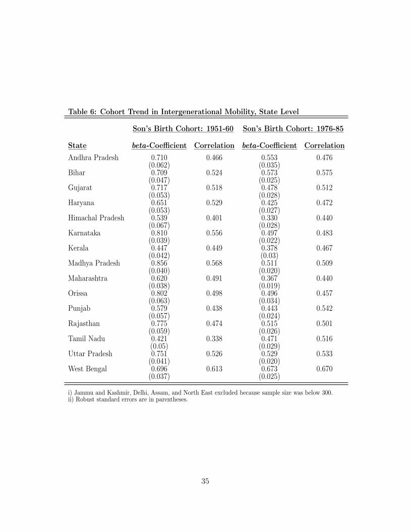
Table 6: Cohort Trend in Intergenerational Mobility, State Level

Son’s Birth Cohort: 1951-60 Son’s Birth Cohort: 1976-85

State beta-Coefficient Correlation beta-Coefficient Correlation

Andhra Pradesh 0.710 0.466 0.553 0.476(0.062) (0.035)

Bihar 0.709 0.524 0.573 0.575(0.047) (0.025)

Gujarat 0.717 0.518 0.478 0.512(0.053) (0.028)

Haryana 0.651 0.529 0.425 0.472(0.053) (0.027)

Himachal Pradesh 0.539 0.401 0.330 0.440(0.067) (0.028)

Karnataka 0.810 0.556 0.497 0.483(0.039) (0.022)

Kerala 0.447 0.449 0.378 0.467(0.042) (0.03)

Madhya Pradesh 0.856 0.568 0.511 0.509(0.040) (0.020)

Maharashtra 0.620 0.491 0.367 0.440(0.038) (0.019)

Orissa 0.802 0.498 0.496 0.457(0.063) (0.034)

Punjab 0.579 0.438 0.443 0.542(0.057) (0.024)

Rajasthan 0.775 0.474 0.515 0.501(0.059) (0.026)

Tamil Nadu 0.421 0.338 0.471 0.516(0.05) (0.029)

Uttar Pradesh 0.751 0.526 0.529 0.533(0.041) (0.020)

West Bengal 0.696 0.613 0.673 0.670(0.037) (0.025)

i) Jammu and Kashmir, Delhi, Assam, and North East excluded because sample size was below 300.ii) Robust standard errors are in parentheses.

35

Table 7: Intergenerational Transitional Probabilities, All India

Panel A- Son’s Birth Cohort: 1951-55

Son’s Education:

< Primary Primary Middle School Secondary Post Secondary size

Father’s Education:

< Primary 0.501 0.185 0.119 0.123 0.071 0.773Primary 0.099 0.234 0.207 0.215 0.245 0.112Middle 0.046 0.052 0.293 0.308 0.301 0.044Secondary 0.029 0.035 0.114 0.376 0.446 0.041Post Secondary 0.017 0.030 0.070 0.081 0.802 0.030

Panel B- Son’s Birth Cohort: 1981-85

Son’s Education:

< Primary Primary Middle School Secondary Post Secondary size

Father’s Education:

< Primary 0.332 0.217 0.224 0.117 0.110 0.495Primary 0.105 0.198 0.293 0.173 0.231 0.173Middle 0.053 0.105 0.321 0.192 0.330 0.116Secondary 0.024 0.048 0.167 0.238 0.523 0.125Post Secondary 0.008 0.022 0.078 0.165 0.727 0.092

i) Each cell ij represents the average probability (for a given cohort) of father with education level i having a son witheducation attainment level j.ii) Column titled “size” reports the fraction of parents in each education category.

36

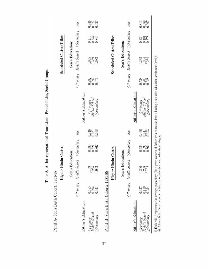
Tab

le8.

A:

Inte

rgen

erat

iona

lT

rans

itio

nal

Pro

babi

litie

s,So

cial

Gro

ups

Pan

elA

-So

n’s

Bir

thC

ohor

t:19

51-5

5

Hig

her

Hin

duC

aste

sSc

hedu

led

Cas

tes/

Tri

bes

Son’

sE

duca

tion

:So

n’s

Edu

cati

on:

≤Pri

mar

yM

iddl

eSc

hool≥S

econ

dary

size

≤Pri

mar

yM

iddl

eSc

hool≥S

econ

dary

size

Fath

er’s

Edu

cati

on:

Fath

er’s

Edu

cati

on:

≤Pri

mar

y0.

455

0.15

90.

386

0.74

6≤P

rim

ary

0.79

20.

095

0.11

30.

946

Mid

dle

Scho

ol0.

094

0.28

50.

621

0.08

7M

iddl

eSc

hool

0.09

70.

359

0.54

40.

027

≥Sec

onda

ry0.

041

0.09

30.

867

0.16

8≥S

econ

dary

0.07

10.

083

0.84

60.

027

Pan

elB

-So

n’s

Bir

thC

ohor

t:19

81-8

5

Hig

her

Hin

duC

aste

sSc

hedu

led

Cas

tes/

Tri

bes

Son’

sE

duca

tion

:So

n’s

Edu

cati

on:

≤Pri

mar

yM

iddl

eSc

hool≥S

econ

dary

size

≤Pri

mar

yM

iddl

eSc

hool≥S

econ

dary

size

Fath

er’s

Edu

cati

on:

Fath

er’s

Edu

cati

on:

≤Pri

mar

y0.

337

0.24

00.

423

0.46

6≤P

rim

ary

0.53

80.

232

0.23

00.

813

Mid

dle

Scho

ol0.

119

0.28

80.

593

0.14

1M

iddl

eSc

hool

0.20

50.

304

0.49

10.

089

≥Sec

onda

ry0.

034

0.10

20.

864

0.39

3≥S

econ

dary

0.08

80.

234

0.67

80.

097

i)E

ach

cellij

repr

esen

tsth

eav

erag

epr

obab

ility

(for

agi

ven

coho

rt)

offa

ther

wit

hed

ucat

ion

leve

liha

ving

aso

nw

ith

educ

atio

nat

tain

men

tle

velj

.ii)

Col

umn

titl

ed“size”

repo

rts

the

frac

tion

ofpa

rent

sin

each

educ

atio

nca

tego

ry.

37

Tab

le8.

B:

Inte

rgen

erat

iona

lT

rans

itio

nal

Pro

babi

litie

s,So

cial

Gro

ups

Pan

elA

-So

n’s

Bir

thC

ohor

t:19

51-5

5

Oth

erB

ackw

ard

Cas

tes

Mus

lim

Son’

sE

duca

tion

:So

n’s

Edu

cati

on:

≤Pri

mar

yM

iddl

eSc

hool≥S

econ

dary

size

≤Pri

mar

yM

iddl

eSc

hool≥S

econ

dary

size

Fath

er’s

Edu

cati

on:

Fath

er’s

Edu

cati

on:

≤Pri

mar

y0.

597

0.14

80.

255

0.93

5≤P

rim

ary

0.80

80.

082

0.11

00.

887

Mid

dle

Scho

ol0.

119

0.23

10.

650

0.02

8M

iddl

eSc

hool

0.11

40.

309

0.57

70.

044

≥Sec

onda

ry0.

100

0.07

10.

829

0.03

8≥S

econ

dary

0.06

60.

231

0.70

30.

069

Pan

elB

-So

n’s

Bir

thC

ohor

t:19

81-8

5

Oth

erB

ackw

ard

Cas

tes

Mus

lim

Son’

sE

duca

tion

:So

n’s

Edu

cati

on:

≤Pri

mar

yM

iddl

eSc

hool≥S

econ

dary

size

≤Pri

mar

yM

iddl

eSc

hool≥S

econ

dary

size

Fath

er’s

Edu

cati

on:

Fath

er’s

Edu

cati

on

≤Pri

mar

y0.

450

0.26

40.

286

0.65

8≤P

rim

ary

0.60

20.

215

0.18

20.

718

Mid

dle

Scho

ol0.

123

0.36

90.

509

0.12

4M

iddl

eSc

hool

0.25

40.

293

0.45

30.

107

≥Sec

onda

ry0.

047

0.10

40.

849

0.21

9≥S

econ

dary

0.10

40.

181

0.71

60.

175

i)E

ach

cellij

repr

esen

tsth

eav

erag

epr

obab

ility

(for

agi

ven

coho

rt)

offa

ther

wit

hed

ucat

ion

leve

liha

ving

aso

nw

ith

educ

atio

nat

tain

men

tle

velj

.ii)

Col

umn

titl

ed“size”

repo

rts

the

frac

tion

ofpa

rent

sin

each

educ

atio

nca

tego

ry.

38

Figure 1: Average and Standard Deviation of years of schooling, ALL India

24

68

1940-45

1946-50

1951-55

1956-60

1961-65

1966-70

1971-75

1976-80

1981-85

Son's Birth Cohort

Average years of schooling

24

68

1940-45

1946-50

1951-55

1956-60

1961-65

1966-70

1971-75

1976-80

1981-85

Son's Birth Cohort

Standard Deviation-years of schooling

Son Father

Figure 2: Ranking India in terms of Intergenerational Mobility

India

0 .2 .4 .6 .8Correlation

PeruPanamaEcuador

ChileColombia

BrazilNicaraguaIndonesia

ItalySlovenia

IndiaEgypt

HungarySri Lanka

USASwitzerland

PakistanIrelandPoland

VietnamSweden

PhilippinesEstoniaUkraineGhana

East TimorSlovakia

Czech RepublicThe Netherlands

NorwayNepal

New ZealandFinland

Northern IrelandMalaysia

Great BritainDenmark

Krygystan

Note: Estimate for India are from Authors’ calculation. Estimates for other nations are from Hertz et al.

(2008), Table 2.

39

Figure 3: Clustering of observations around the Regression line for the OBC

05

10

15

Son's

years

of educa

tion

0 5 10 15Father's years of schooling

1940-45 Cohort

05

10

15

Son's

years

of educa

tion

0 5 10 15Father's years of schooling

1981-85 Cohort

Figure 4: Intergenerational Education Mobility, State Level

Himachal

Punjab

Uttar Pradesh

Haryana

Rajasthan

Bihar

West Bengal

Orissa

Madhya Pradesh

Gujarat

Maharashtra

Andhra Pradesh

Karnataka

Kerala

Tamil Nadu

.3.4

.5.6

.7.8

.91976-8

5 c

ohort

.3 .4 .5 .6 .7 .8 .91951-60 Cohort

Note: Jammu and Kashmir, Delhi, Assam, and Northeast excluded because of smaller sample sizes. See text

for details.

40

Figure 5: Intergenerational Mobility and Public Educational Spending, State Level

5a) Birth Cohort: 1951-60

Andhra PradeshBihar

Gujarat

Haryana

Karnataka

Kerala

Madhya Pradesh

Maharashtra

Orissa

Punjab

Rajasthan

Tamil Nadu

Uttar Pradesh

West Bengal

.1.2

.3.4

.5.6

Ed

ucation

Mo

bili

ty (

1-b

eta

): 1

95

1-6

0 B

irth

Co

ho

rt

2345678910111213141516State rank based on per capita education expenditure 1958-2000

5b) Birth Cohort: 1976-85

Andhra Pradesh

Bihar

Gujarat

Haryana

Karnataka

Kerala

Madhya Pradesh

Maharashtra

Orissa

Punjab

Rajasthan

Tamil Nadu

Uttar Pradesh

West Bengal

.3.4

.5.6

.7E

ducation

Mo

bili

ty (

1-b

eta

): 1

97

6-8

5 B

irth

Co

ho

rt

2345678910111213141516State rank based on per capita education expenditure 1958-2000

Note: Jammu and Kashmir was ranked 1 in terms of per capita education spending. However, our analysis

excludes this state due to smaller sample size.

41

Appendix A: Co-residence condition and Sample Selection in the NSS

In this section, we illustrate the sample selection issues that may arise due to the identifica-

tion of father-son pairs based on co-residence. Using the 61st round of the NSS (2004-05), we

first show that the sample of adult males that can be matched with their father’s information

using the co-residence condition disproportionately represents younger individuals. Then,

we also show that even one concentrates on relatively younger cohorts (i.e. restricting the

analysis to only younger cohorts, such as 20-30 age group), the persons for whom father’s

information is identified may not be a random subsample of the concerned age group.

Table A.1: Distribution of population aged 20-65 based on the relationship to head, NSS 2004-05

Relation to the Head (Code) Relation to the Head Sample Size

Male Female

1 Self 101,053 12,2842 Spouse of head 338 96,7213 Married child 25,954 2,7204 Spouse of married child 881 25,8235 Unmarried child 24,927 10,8456 Grandchild 1,111 6627 Father/ mother/ father-in-law/ mother-in-law 1,296 7,5568 Brother/ sister/ brother-in-law/ sister-in-law/ other relatives 7,314 5,8609 Servants/ employees/ other non-relatives 564 203

Total 163,438 162,674

Source: NSS 61st Round Employment and Unemployment Survey, 2004-05

In the NSS data set (similarly, in the NFHS), parents identification is achieved through

imposition of co-resident condition and exploiting the “relationship to head” information.

Table A.1 provide the information on the various types of relationship captured in this vari-

able and the corresponding sample sizes in the 2004-05 round of the NSS.32 As is evident

from the sample sizes reported in Table A.1, using co-residence to identify father’s informa-

tion would lead to severe loss of observations. This is because almost 62 percent of adult

32In the NFHS (2005-06), “relation to head” has following categories: 1-self, 2-wife or husband,3-son/daughter, 4-son/daughter-in-law, 5-grandchildren, 6-parents, 7-parents-in-law, 8-brother/sister, 9-brother/sister-in-law, 10-niece/nephew, 11-other relatives, 12-adopted/foster/step child, 13-domestics ser-vants, 14-other non relatives.

42

male sample consist of household’s head whose father information is not available. One can

potentially identify fathers’ for only those male persons in age 20-65 who has reported rela-

tionship to head as married/unmarried child (50,881 individuals or 31 percent of the entire

adult male population). Hence males in age 20-65 who reported as child of head can be

matched to head if head is male or with spouse (if alive and co-resident) of head if head is

female. Out of 50,991 persons who reported as child of head, 44,228 live in male headed

households, while 6,653 live in female headed households. However, 6508 female headed

households do not have spouse of head living in household. Hence, through co-resident,

we could identify father’s education only for 44,373 males in age 20-65, which is merely 27

percent of the total males in age 20-65.

Figure A.1: Age distribution of males in the age group 20-65, NSS 2004-05

0.1

.2.3

Frac

tion

20 25 30 35 40 45 50 55 60 65 Age

Sample Size: 163,438

All males

0.1

.2.3

Frac

tion

20 25 30 35 40 45 50 55 60 65 Age

Sample Size: 44,350

Males whose fathers' education is identified

Note: Survey weights are used to get the age distribution.

Figure A.1 presents the age distribution of male in the age group 20-65 for the entire

sample and for the co-resident sample (matched with their father using the co-residence con-

dition). As we observe from this figure, there are significant difference in the age distribution

of the two samples. Specifically, a large majority of the co-resident sample is concentrated in

the 20-30 age group (roughly 80 percent). Hence, using co-residence we have an oversample

of younger adults which is expected as these individuals are more likely to be residing with

their parents.

43

Figure A.2: Proportion in each age group (male) whose father education is identified in theNSS, 2004-05

020

4060

8010

0Pe

rcenta

ge wh

ose fa

thers

educa

tion is

identif

ied

20-25 26-30 31-35 36-40 41-45 46-50 51-55 56-60 61-65

Note: Survey weights are used to calculate the proportions.

In addition to having a non-representative sample of the adult male population, the

father’s education information identified in each age group may not be randomly distributed

across observations. In Figure A.2, we plot the proportion in each age group (male) whose

father education is identified using the co-resident sample from the 2004-05 NSS round.

Again, we find that in the co-resident sample, although the percentage of individuals whose

father’s education can be identified are much higher for the younger age groups, it remains

a non random sub sample of that particular age group. As a result, not only the estimates

(cross-section estimates) of intergenerational mobility based on the father-son pair identified

through co-residence would be biased, but also the bias will not be eliminated even if one

concentrate on only younger age groups.

44

Appendix B: Evolution of Education Policy in India

Table B: Education Policy in India 1951-2005

Period Policy Framework Policy Measures and Programmes

1951-68 Constitution Expansion of the formal schooling system. State governmentsof India shoulder the responsibility for primary education.

1968-86 National Policy on 1976: Education shifted to the Concurrent list therebyEducation, 1968 giving the GOI and state governments equal

responsibility for promoting and managing education.1980s: Non-Formal Education introduced to supplementformal schooling, thereby increasing Central investmentin primary schooling.

1986-92 National Policy on Andhra Pradesh Primary Education Project, early 1980Education, 1986 (British ODA) Environmental Education, 1986Jomtien Conference (Domestic Resources) Rajasthan Shiksha Karmi Project,for Education for All, 1987 (Sida) Total Literacy Campaign, 1988followed by EFA (Domestic resources) Mahila Samakhya in Karnataka,projects most of UP and Gujarat, 1989 (Dutch Government) Biharthem with foreign Education Project, 1991 (UNICEF) Rajasthan Lok Jumbish, 1992 (Sida)aid UP Basic Education Project, 1992 (World Bank)

1992-2002 Revised National District Primary Education Programme (DPEP), 1993Policy on Education National Programme of Nutritional Support to Primary EducationMid-day meal, 1995, (Mid Day Meal), 1997, Sarva Shiksha Abhiyan, 2001Supreme Court Orderon Mid-day meal, 2001

2002 onwards Free and compulsory Free and Compulsory Education made fundamental right of childreneducation bill, 2004 in the age group 6-14Revised Mid-day meal Universal Mid-day meal across primary schools in the countryProgramme in 2004

Source: Ensuring Universal Access To Health and Education In India, November 2007.

45