Likelihood based inference for diffusion driven state space

models

Siddhartha Chib

Olin School of Business, Washington University, St Louis

Michael Pitt

Department of Economics, University of Warwick

Neil Shephard

Oxford-Man Institute, University of Oxford

AND

Department of Economics, University of Oxford

September 2010

Abstract

In this paper we develop likelihood based inferential methods for a novel class of(potentially non-stationary) diffusion driven state space models. Examples of models inthis class are continuous time stochastic volatility models and counting process models.Although our methods are sampling based, making use of Markov chain Monte Carlomethods to sample the posterior distribution of the relevant unknowns, our generalstrategies and details are different from previous work on related but simpler models.The proposed methods are easy to implement and simulation efficient. Importantly,unlike methods for related models, the performance of our method is not worsened as thedegree of latent augmentation is increased to reduce the bias of the Euler approximation.We also consider the problems of model choice, model checking and filtering and applythe techniques and ideas to both simulated and real data.

Keywords: Bayes estimation, Brownian bridge, Non-linear diffusion, Euler approxima-

tion, Markov chain Monte Carlo, Metropolis-Hastings algorithm, Missing data, Simulation,

Stochastic differential equation.

1 Introduction

1.1 The diffusion driven state space class

In many areas of science, it is common to model a continuous outcome in terms of a diffusion

process (namely, a continuous time process), wherein the increments of the outcome over an

infinitesimal interval are governed by the increments of a Weiner process. The continuous

time stochastic evolution of the process can then equivalently be described by a nonlinear

stochastic differential equation (SDE). A problem of considerable practical and theoretical

relevance is the estimation of the parameters of such diffusions given that the outcome is

1

observed only at discrete time points. In this paper we study the same problem but in

the context of a class of (multivariate) diffusions that is more general than the families of

univariate and multivariate diffusions that have been considered in the past. We call our

family the diffusion driven state space family.

Our model and setting may be described as follows. We observe the continuous outcome

Yi at the non-stochastic times τi for i = 1, 2, ..., n, where

0 = τ0 ≤ τ1 ≤ τ2 ≤ ... ≤ τn ≤ τn+1 = T.

We assume that Y is related to an unobserved underlying d− dimensional (multivariate)

continuous time process α(t) = (α1(t), ..., αd(t))′ for t ≥ 0. Our central assumption is that

conditionally on the sample path of α over the interval t ∈ [τi−1,τi) the observations are

independent with known density

dF (Yi| {α(t); t ∈ [τi−1,τi)} , θ), i = 1, 2, ..., n, (1)

indexed by the unknown vector parameter θ. We complete the model by assuming that the

continuous-time stochastic behavior of α(t) is governed by a multivariate diffusion process

which satisfies the SDE

dα(t) = µ{α(t), θ}dt+Υ{α(t), θ}dW (t), t ∈ [0, T ], (2)

whereW (t) = (W1(t), ...,Wd(t))′ is a d-dimensional vector of independent Weiner processes,

and µ : d× 1 and Υ : d× d are the vector drift and matrix volatility functions, respectively,

such that µ is a function of α(t) and θ, and Υ is a function of α(t). We also suppose that

µ and Υ satisfy the Lipschitz conditions (e.g. Revuz and Yor (1999, p. 375)).

It is possible to view our model in the spirit of a state space model (e.g. West and

Harrison (1997), Harvey (1989), Durbin and Koopman (2001)), with a non-Gaussian mea-

surement density (1) and a Markov transition equation (2). The key twist is that the state

α(t) is governed by a non-linear continuous time process, while the i-th measurement den-

sity can depend upon the entire path of α in the time interval [τi−1,τi) which makes our

model more general than those which have been considered before.

The diffusion driven state space class is quite general and covers many common diffusion

based models. Here we list some examples and discuss the variety of methods researchers

have developed to handle these particular cases.

Example 1 Stochastic volatility. (e.g. Ghysels, Harvey, and Renault (1996) and Shep-

hard (2005)). Suppose a univariate log-price process P follows the diffusive stochastic

2

volatility (SV) process

dP (t) ={θ1 + θ2σ

2(t)}dt+ σ(t)dB(t), (3)

where σ2(t) = exp {α(t)}. Such processes appear extensively in financial econometrics.

Assume that B and W are standard Brownian motions with

Corr(B(t),W (t)) = ρ

and that we record returns

Yi = P (τi)− P (τi−1), i = 1, 2, ..., n.

Then

Yi| {α(t); t ∈ [τi−1,τi)} ∼ N(θ1 (τi − τi−1) + θ2σ

2i + ρZi,

(1− ρ2

)σ2i), (4)

where

σ2i =

∫ τi

τi−1

σ2(u)du, Zi =

∫ τi

τi−1

σ(u)dW (u). (5)

The problem of carrying out inference for this kind of hidden factor model was the motiva-

tion for the work of Smith (1993), Gourieroux, Monfort, and Renault (1993) and Gallant and

Tauchen (1996) on indirect inference and efficient method of moments methods while from

the Bayesian Markov chain Monte Carlo perspective, Kim, Shephard, and Chib (1998), Ele-

rian, Chib, and Shephard (2001) and Eraker (2001) showed how an augmentation approach

could reduce the discretisation bias of the Euler approximation.

Example 2 Counting process. Suppose N is a one dimensional counting process ob-

tained by time changing a standard, homogeneous Poisson process N∗. Assume that the

time change is of the form∫ t

0 λ(u)du where λ ⊥⊥ N∗ and λ is some function of the multi-

variate univariate α. Here ⊥⊥ denotes stochastic independence. In this set-up,

E(N(t+ dt)−N(t)|α(t)) = λ(t)dt,

so that λ can be thought of as the spot intensity of N . Then

Yi = N(τi)−N(τi−1)

and

Yi| {α(t); t ∈ [τi−1,τi)} ∼ P

(∫ τi

τi−1

λ(u)du

).

Thus N is a Cox (1955) process (or a doubly stochastic processes). Models of this type are

used in the modeling of credit risk (e.g. Lando (1998) and Duffie and Singleton (1999)),

internet traffic, insurance and image analysis.

3

Example 3 Linear Gaussian state space models. Harvey (1989, Ch. 9) provides a

discussion of continuous time linear Gaussian unobserved component models. An example

of such a model is given by

Yi = α(τi) + εi, εi ∼ NID(0, σ2ε ),

where α is a Brownian motion process that is independent of ε. A slight variant on this is

the model in which the signal is the average value of the state

Yi =1

τi − τi−1

∫ τi

τi−1

α(u)du+ εi, εi ∼ NID(0, σ2ε ).

Another variant is the cubic spline model (e.g. Wecker and Ansley (1983) and Harvey

and Koopman (2000)). All these models can be exactly discretised and placed into the

linear, Gaussian state space form. Inference can be handled by the Kalman filter, smoother

and simulation smoother methods. This allows us to deal with irregularly spaced data

from linear, Gaussian models, a point made by Jones (1984), Harvey and Stock (1985) and

Harvey and Stock (1988). Our analysis can be viewed as the non-linear and non-Gaussian

extension of this work.

An important point to note is that the fitting of diffusion models of the foregoing type

is not straightforward and a number of methods have been explored and studied. Gallant

and Tauchen (2004), Bibby, Jacobsen, and Sørensen (2004) and Aıt-Sahalia, Hansen, and

Scheinkman (2004)) provide useful reviews of moment based methods. Likelihood-based

methods, implemented typically by simulation, are developed in eg. Pedersen (1995), Ele-

rian, Chib, and Shephard (2001), Durham and Gallant (2002), Ait-Sahalia (2002), and Ait-

Sahalia (2003)). Bayesian methods, which rely on the idea of data augmentation, appear in

Elerian, Chib, and Shephard (2001), Roberts and Stramer (2001) and Eraker (2001). Like-

lihood methods that parallel the Bayesian approach are outlined by Durham (2003), Brandt

and Santa-Clara (2002), Nicolau (2002) and Hurn, Lindsay, and Martin (2003). Finally, im-

portant recent contributions that develop simulation-based methods for special cases of our

models are Beskos and Roberts (2005), Beskos, Papaspiliopoulos, Roberts, and Fearnhead

(2006) and Beskos, Papaspiliopoulos, and Roberts (2009). Recent work on latent diffusion

models, relying on time change transformations, has been undertaken by Kalogeropoulos

(2007) and Kalogeropoulos, Roberts, and Dellaportas (2010). These methods depend on

a transformation of (2) to make the volatility term independent of the states. This is not

always straightforward to do for general multivariate diffusions and our approach does not

need this transformation.

4

1.2 Outline of the paper

In Section 2 we begin by outlining our approach to inference for the diffusion driven state

space family of models. Although our general approach is sampling based, making use of

Markov chain Monte Carlo methods to sample the posterior distribution of the relevant

unknowns, the general strategies and details are different from previous work. We regard

the parameters as fixed and known. We illustrate the effectiveness of our method and show

that the performance of our method is not worsened as the degree of latent augmentation

is increased to reduce the bias of the Euler approximation. In Section 3 we consider the

problem of sampling the parameters from the posterior distribution. We propose a new

scheme which samples the parameters (or a subset of the parameters) given the Brownian

motion driving the latent process. As we are sampling blocks of the latent diffusion in time,

the resulting Markov chain method can no longer be regarded as a standard Metropolis

within Gibbs method. We prove that the invariant distribution resulting from our method

is, however, correct. The proof associated with the method of Section 3 is given in Section

7.1. To our knowledge this is a new contribution. In Section 4 we consider two applications.

The first application, in Section 4.1, is a simulated two factor model for volatility. This is

a challenging problem in that the two components for volatility mix at quite different rates

(one very slowly and one very quickly). The resulting MCMC algorithm needs to take this

into account to sample the latent volatilities efficiently. The second application, in Section

4.2, apply our methods to fit a volatility model with leverage using data on the Standard

and Poor’s stock index. We consider and compare a three different models for volatility.

Section 5 contains our concluding remarks. An appendix collects the prior distribution we

use in some of our examples along with the particulars of the MCMC sampling schemes

that are not given in the main body of the paper.

2 Augmentation and inference

2.1 The basic framework

In our general approach we combine a prior distribution π(θ) of θ with the likelihood of the

observations Y = (Y1, ..., Yn) to produce the posterior distribution

θ|Y. (6)

Unfortunately the likelihood function for diffusion driven model is not known, except in some

simple cases such as those in Example 3. We side step the computation of the likelihood

function by augmenting θ with the entire path of α from time 0 to T . We then employ

5

MCMC methods (eg., Chib (2001)) to sample from the infinite dimensional posterior density

θ, {α(t); t ∈ [0, T ]} |Y. (7)

If we do this many times and just record the values of θ, we get a sample from (6) and

thereby estimates of any posterior quantity of interest, e.g. posterior means, quantiles and

covariances. It may be noted that the general idea of augmentation in this context emerges

from Kim, Shephard, and Chib (1998), Elerian, Chib, and Shephard (2001), Eraker (2001)

and Roberts and Stramer (2001), but our strategy and details are different.

We now show how it is possible to design MCMC samplers which draw from (7).

Algorithm 2.1.

1. Sample from {α(t); t ∈ [0, T ]} |θ, Y by updating the subsets of the sample path.

(a) Randomly split time from 0 to T into K+1 sections. We write these subsampling

times as

0 = t0 ≤ t1 ≤ t2 ≤ ...tK ≤ tK+1 = T,

and collect all Y observations and their subscripts which appear in the interval

of time [tk−1,tk]. These will be labelled {k} and Y{k} for k = 1, 2, ...,K + 1.

(b) Sample the subpath

{α(t); t ∈ [tk−1, tk]} |Y{k}, θ, α(tk−1), α(tk), k = 1, 2, ...,K + 1. (8)

2. Draw from

θ|Y, {α(t); t ∈ [0, T ]} .

3. Goto 1.

The resulting draws obey a Markov chain whose equilibrium marginal distribution is

(7). All inferences are based on these sequences, beyond a suitable burn-in. Of course, the

draws are serially correlated and therefore not as informative as i.i.d. draws from (7). We

measure this dependence by the so-called inefficiency factor (autocorrelation time) of each

posterior estimate. This measure, written INF (L), is defined as 1+2∑L

i=1 ρ(i), where ρ(i)

is the autocorrelation at lag i and L is a truncation point. See also Geweke (1989) who

prefers to report the inverse of this number. By way of interpretation, to make the variance

of the posterior estimate the same as that from independent draws, the MCMC sampler

must be run INF (L) times as many iterations, beyond the transient phase of the Markov

chain.

6

In implementing this strategy the main issue is how to sample from variables of the type

(8). To do this we will first develop methods for making proposals for the sub-path

{α(t); t ∈ [tk−1, tk]}

drawn from

{α(t); t ∈ (tk−1, tk)} |Y{k}, θ, α(tk−1), α(tk), (9)

which is a multivariate non-linear bridge diffusion. This problem has recently been explored

by Beskos, Papaspiliopoulos, Roberts, and Fearnhead (2006) who derive efficient algorithms

for some specific classes of diffusions.

Carrying out the simulation from (9) directly is difficult due to the fact that we are

conditioning on the end-point α(tk). Instead, we simulate from a rather similar process —

rejecting some of these proposals in order to correct for the resulting error. Consider the

alternative diffusion α∗, which is constructed to have the following four properties

• It only exists on the time interval [tk−1, tk].

• It starts at α∗(tk−1) = α(tk−1).

• It finishes α∗(tk) = α(tk).

• It has the same volatility function as the α process.

We are rather free to select the drift function of α∗, so we use the simple form

dα∗(t) = {tk − t}−1 {α(tk)− α∗(t)} dt+Υ {α∗(t)} dW (t) (10)

= µ∗{α∗(t)}dt+Υ {α∗(t)} dW (t), (11)

where we have suppressed the dependence of the drift on t.

Due to the common volatility function the models (2) and (10) deliver locally equivalent

measures P and Q, respectively. The resulting likelihood ratio LP,Q(α|θ) is given by the

Girsanov’s formula (Øksendal (1998, p. 147)) for the path {α(t); t ∈ [tk−1, tk]},

logLP,Q(α|θ) =∫ ti

ti−1

(µ (α)− µ∗ (α))′Σ−1 (α) dα (12)

− 1

2

∫ ti

ti−1

(µ (α)− µ∗ (α))′ Σ−1 (α) (µ (α)− µ∗ (α)) du,

where Σ = ΥΥ′. Beskos and Roberts (2005) show that it is sometimes possible to use this

likelihood ratio inside a rejection algorithm to sample from the tied down version of (2) by

7

making proposals from (10). However, in general this is not possible and we have to resort

to MCMC methods.

We generate a path from P by using proposals from Q with the help of an Metropolis-

Hastings algorithm (for details of the algorithm see, for example, Chib and Greenberg

(1995)). Reintroducing the conditioning Y{k} is straightforward. The resulting algorithm

has the following form.

Algorithm 2.2

1. Set j = 1. Calculate some initial stretch{α(0)(t); t ∈ [tk−1, tk)

}which obeys the end

point constraints α(tk−1), α(tk).

2. Propose the subpath{α(j)(t); t ∈ [tk−1, tk)

}by sampling from (10).

3. Accept proposal with probability

min

[1,

dF(Y{k}|α(j), θ

)

dF(Y{k}|α(j−1), θ

) LP,Q(α(j)|θ)

LP,Q(α(j−1)|θ)

],

otherwise write

{α(j)(t); t ∈ [tk−1, tk)

}={α(j−1)(t); t ∈ [tk−1, tk)

}.

4. Set j = j + 1. Goto 2.

The density

dF(Y(k)|α, θ

)=∏

i∈(k)

dF (Yi|α, θ)

=∏

i∈(k)

dF (Yi| {α(t); t ∈ [tk−1, tk)} , θ)

is straightforward to evaluate by the assumption of the model. The remaining issues are

simulating from (10) and computing LP,Q(α|θ).

2.2 Numerical implementation

It is easy to accurately sample from the crucial (10) using a high frequency Euler ap-

proximation (e.g. Kloeden and Platen (1992) and Jacod and Protter (1998)). The Euler

approximation of (10) is

αk,j|αk,j−1, θ ∼ N (αk,j−1 + δµ∗ (αk,j−1) , δΣk,j−1) , j = 1, 2, ...,Mk , (13)

8

where Mk ≥ 1 is a large positive integer, δ = (tk − tk−1) /Mk, Σk,j = Σ(αk,j) and

αk,j = α(tk−1 + δj), j = 0, 1, 2, ...,Mk .

The function µ∗{α(t)}, introduced in equation (10) and (11), again also implicitly includes

the end point, now αk,Mk. This Euler approximation contrasts with an Euler approximation

of the true process (2), which has

αk,j|αk,j−1, θ ∼ N (αk,j−1 + δµ (αk,j−1) , δΣk,j−1) . (14)

We write the conditional density of (14) as pN (αk,j|αk,j−1, θ), while using qN (αk,j|αk,j−1, θ)

for the corresponding one for (13).

Remark 1 In the univariate case this is the same as the proposal process for the impor-

tance sampler of Durham and Gallant (2002). An extensive explanation of this importance

sampler is given in Chib and Shephard (2002).

Writing µk,j = µ (αk,j) and µ∗k,j = µ∗ (αk,j) then logLP,Q(α), of (12), is approximated

by

log LP,Q(α|θ) =Mk∑

j=1

(µk,j−1 − µ∗k,j−1

)′Σ−1k,j (αk,j − αk,j−1)

− 1

2δ

Mk∑

j=1

(µk,j−1 − µ∗k,j−1

)′Σ−1k,j

(µk,j−1 − µ∗k,j−1

),

which we express as

log LP,Q(α|θ) =Mk∑

j=1

(log pN (αk,j |αk,j−1, θ)− log qN (αk,j|αk,j−1, θ)). (15)

Clearly log LP,Q(α|θ) converges in probability to logLP,Q(α|θ) as Mk → ∞ using standard

properties of the Euler approximation.

Remark 2 For a fixed Mk, equation (15) shows the connection between this method and

those of Elerian, Chib, and Shephard (2001) and Eraker (2001) in the pure diffusion case.

Both these papers sample from the log-density

Mk∑

j=1

log pN (αk,j|αk,j−1, θ),

tied down by αk,0 = α(tk−1) and αk,Mk= α(tk). Elerian, Chib, and Shephard (2001)

made multivariate proposals using a Laplace type approximation, which was computationally

9

intensive but effective. Instead we now adopt the simpler approach of proposing blocks using

(13), which is easier to code and numerically faster and better behaved asMk → ∞. Further,

our analysis shows that a well designed proposal process should produce an excellent MCMC

algorithm as the Metropolis-Hastings acceptance probability does not go to zero as Mk →∞. Eraker (2001) advocated a rather different approach. He favoured running MCMC

chains inside these blocks, updating a single αk,j at a time, conditional on its neighbours.

Although this algorithm is as simple to code as our new approach and runs as quickly, it

produces output that is more serially correlated. Indeed, Elerian (1999) proved that the rate

of convergence of the Eraker (2001) algorithm worsens linearly with Mk.

WhenMk is small it is quite possible that our proposal is not an outstandingly good one,

due to the non-linearity in the diffusion. Thus, it may be beneficial to replace the Gaussian

assumption in the proposal (13) with a heavier tailed alternative such as the multivariate-t.

This requires a corresponding, but simple, adjustment in (15). In practice for the examples

we have computed in this paper the data is equally spaced so that δ = (tk − tk−1) /M and

M is constant.

2.3 Numerical example: stochastic volatility

A simple log-normal SV model puts

dP (t) = θ1dt+ σ(t)dB(t), (16)

a special case of (3) with θ2 = 0. We assume that the log volatility, α(t) = log{σ2(t)

},

follows the Ornstein-Uhlenbeck (OU) diffusion,

dα(t) = −θ4(α(t) − θ5)dt+ θ3dW (t), (17)

where ρ = Corr(B(t),W (t)). Here θ1 parameterises the drift of the P , θ5 the general

level of volatility, θ3 the volatility of the volatility, θ4 the persistence of volatility and,

finally, ρ the degree of leverage. In our experiments we will take θ1 = 0.03, θ3 = 0.125,

θ4 = {0.0137, 0.1, 1.386} , θ5 = 0 and ρ = −0.620. These parameter values are taken from

the empirical work on U.S. equity returns reported in Andersen, Benzoni, and Lund (2002),

Andersen, Bollerslev, and Diebold (2007) and Chernov, Gallant, Ghysels, and Tauchen

(2003). It copies the Monte Carlo design of Huang and Tauchen (2005). The three possible

values of θ4 represent slow, medium and fast mean reversion, respectively. In this experiment

we will fix the parameter values at their true values, simulate the process and then study

the autocorrelation of the sampler for α|Y, θ. We let M take the values 1, 4, 10 and 50 and

T the value 100. For simplicity of exposition we will let t = 1 represent one day.

10

For this model returns Yi = P (i)− P (i− 1), arise from

Yi|α(t); t ∈ [i− 1, i), θ ∼ N(θ1 + ρZi,

(1− ρ2

)σ2i),

a restricted version of (4) where operationally in our algorithm,

σ2i =1

M

M∑

j=1

exp (αi,j) , Zi =

M∑

j=1

exp (αi,j/2) (Wi,j+1 −Wi,j) . (18)

These are the Euler discretised analogues, see Section 2.2, of (5) with Wi,0 = 0. Note

the values of the Wi,j can be deduced from the values of the αi,j given knowledge of the

parameters.

Our results are based on 10, 000 MCMC draws collected after a burn-in of a 100 cycles.

The computation time is basically proportional toM . Figure 1 shows the average acceptance

rate and the statistical inefficiency (relative to a hypothetical independent sampler) from

the M-H step for the state sampling algorithm with the displayed subsampling times on

the interval (0; 100). The figure is given for the different values of M and for the different

persistency rates determined by θ4. We sample trajectories of α(t) using Algorithm 2.1.

Our blocking method samples α(t) over blocks of time (taking a random block size with

each M-H sweep) with the average time block size being 10. For example, a typical block

might be α(t) for t ∈ (11.2, 21.5). Hence in the M = 50 case we are proposing moves in

our M-H step of average dimension 500. In line with our expectations from Section 2.2, the

efficiency and acceptance rates are independent of the choice of M . Indeed, for the very low

persistence case θ4 = 1.386 we do noticeably better by increasing M from 1. In addition

to the invariance of our algorithm with respect to the degree of augmentation, we have

a scheme which is highly efficient in absolute terms. The inefficiency (measured through

integrated autocorrelation time) from our method is about 10 which is highly efficient in

models of this type. There is a theoretical discussion of less efficient single move procedures,

for discrete time models, in Pitt and Shephard (1999a).

2.4 General procedures

In some high dimensional problems it may be necessary to use more general procedures for

imputing the unknown state α(t) over time. The previous section describes an approach for

imputing the entire latent state (for fixed intervals of time) when we know the measurement

density conditional on the path of the state over this interval, given by (1). In some

applications, see for instance Section 4.1, we may wish to impute the missing observations

(the price process in that example) and to be able to sample parts of the state space

11

0 20 40 60 80 100

0.5

0.6

0.7

0.8M = 1 M=10

M=4 M=50

0 20 40 60 80 100

10

15M=1 M=10

M=4 M=50

0 20 40 60 80 100

0.7

0.8

0.9M=1 M=10

M=4 M=50

0 20 40 60 80 100

5

10

15M=1 M=10

M=4 M=50

0 20 40 60 80 100

0.25

0.50

0.75

1.00M=1 M=10

M=4 M=50

0 20 40 60 80 100

10

20

30

40M=1 M=10

M=4 M=50

Figure 1: Numerical example: Fixed parameter log-OU stochastic volatility with T=100.Persistence parameter θ4 = 0.0137 (TOP), 0.1 (MIDDLE),1.386 (BOTTOM). DisplayedMetropolis acceptance proportions (LEFT) and inefficiency etimates (RIGHT) for augmen-tation M = 1, 4, 10 and 50. Horizontal axis represents actual time from 0 to 100.

conditional upon other parts. In the example of Section 4.1 we have a two dimensional latent

volatility process v1(t) and v2(t) which are very high persistence and very low persistence

processes respectively. In this case, as we shall see later, it is very useful to be able to

sample v1|v2;Y and v2|v1;Y .

Details of this alternative algorithm, used in Section 4.1, for the sampling of the states

is given in Section 7.3.

3 Algorithm for parameter sampling

3.1 Basic approach

The sole remaining problem for handling diffusion driven models is the step for sampling

from

θ|Y, {α(t); t ∈ [0, T ]} .

At this point it is helpful to parameterise the diffusion component as

dα(t) = µ{α(t);ψ}dt +Υ{α(t);ω}dW (t), t ≥ 0, (19)

12

where θ = (λ′, ψ′, ω′)′, where λ represents parameters in the measurement equation for Y

conditional upon the path of α, given by (1).

We initially think of ω as known, when the log-likelihood for the path of {α(t); t ∈ [0, T ]}is given by Girsanov’s formula

logf(α|ψ)f(α|ψ∗)

=

∫ T

0[µ{α(t);ψ} − µ{α(t);ψ∗}]′Σ−1 {α(t)} dα(t)

− 1

2

∫ T

0[µ{α(t);ψ} − µ{α(t);ψ∗}]′ Σ−1 {α(t)} [µ{α(t);ψ} − µ{α(t);ψ∗}] dt.

We can use this inside a M-H algorithm to appropriately sample from

ψ|ω, λ, α.

The sampling of the measurement parameters λ from

π(λ|α, Y, ψ, ω) ∝ π(λ)

n∏

i=1

dF (Yi| {α(t); t ∈ [τi−1,τi)} ;λ, ψ, ω)

is usually also simple.

The difficulty arises principally in sampling the volatility parameter, ω of (19). The

problem is that the sample path of α exactly gives us the integral of the volatility function

through the quadratic variation of the diffusion

[α](t) =

∫ T

0Υ{α(u);ω}Υ{α(u);ω}′dt.

In many cases this is likely to mean that we can deduce ω from α and therefore ω|α,ψ may

well be degenerate, which implies that the MCMC method will not converge. This feature

was pointed out in the context of univariate diffusions by Roberts and Stramer (2001) and

we call it the Roberts-Stramer critique of this method.

Of course, in practice the sampling schemes above are implemented via an Euler scheme,

applied in conjunction with M augmented points. The critique is less binding when M is

small, which explains why writers like Eraker (2001) and Eraker, Johannes, and Polson

(2003) have not really remarked on it. However, when M is substantially large, as in

our algorithm, the possibility of degeneracy of the conditional distribution of ω becomes

increasingly likely, regardless of what happens in step 1 of Algorithm 2.1. It is therefore

important to have a generic solution to this problem, which we now supply.

3.2 A reparameterisation

In the discussion thus far we have focused on ways to sample from α, θ|Y1, ..., Yn, however,we can alternatively sample from

θ, {W (t); t ∈ [0, T ]} |Y1, ..., Yn,

13

the posterior of the parameters and the driving Brownian process. This is particularly

important for the elements of θ which enter into the volatility function which we have

labelled ω. We write the prior for θ as π(θ). At first sight this looks like the same problem

because the addition of θ to the path of W yields the path of α. In fact, the resulting

MCMC algorithm (which we refer to as the innovation scheme) is subtly different.

Algorithm 3.2.

1. Sample from {W (t); t ∈ [0, T ]} |θ, Y1, ..., Yn by updating the subsets of the sample path.

2. Draw from

θ| {W (t); t ∈ [0, T ]} , Y1, ..., Yn.

3. Goto 1.

Step 1 is carried out using Algorithm 2.1. Conditional upon θ we convert {α(t); t ∈ [0, T ]}to obtain {W (t); t ∈ [0, T ]}. This is not a standard Gibbs-type method when applied to W .

However, since, conditional on θ, there is a one-to-one relationship between W and α over

t ∈ [0, T ] it is valid to take a Gibbs sample of α and convert it into W . The remaining task

is to sample from θ|W,Y1, ..., Yn. Generically this could take the following form.

2a. Combine θ(j−1) and W to construct a path α(j−1).

2b. Propose θ(j) from some density g(θ) which could depend upon Y , W and θ(j−1). Use

θ(j) and W to construct a path α(j). Accept the proposal with probability

min

1,g(θ(j−1))

g(θ(j))

n−1∏

k=1

dF(Yk+1|Yk, α(j), θ(j)

)π(θ(j))

n−1∏

k=1i

dF(Yk+1|Yk, α(j−1), θ(j−1)

)π(θ(j−1))

.

2c. If the proposal is rejected write θ(j) = θ(j−1).

The innovation scheme algorithm is rather simple and overcomes the Roberts-Stramer

critique. In practice we have tended to propose θ using a Laplace approximation to the

conditional posterior {n−1∏

k=1

dF(Yk+1|Yk, α(j), θ

)}π(θ).

Whilst we have described this technique in continuous time, it is implemented using the finite

dimensional Euler discretisation. As the algorithm is not a standard Gibbs (or Metropolis

14

within Gibbs) approach it is not obvious that it will necessarily lead to the correct invariant

distribution. However, we demonstrate that in fact the invariant distribution is correct

provided that step (1) in Algorithm 3.2 involves a valid MCMC scheme for the original α.

The proof of the validity of this algorithm for a finite dimensional problem is provided in the

Appendix, see Proposition 3 in Section 7.1. Clearly although the models and methodology

in this paper are largely presented in continuous time the implementation is carried out

using the finite dimensional Euler approximation. The proof is a new result as far as we

are aware and may be of use in general statistical models.

3.3 Numerical example: stochastic volatility

We return to subsection 2.3 where we sampled from α|Y, θ for the log-normal SV model,

but add the risk premium θ2,

dP (t) ={θ1 + θ2σ

2(t)}dt+ σ(t)dB(t),

dα(t) = −θ4 {α(t)− θ5} dt+ θ3dW (t),

where the log volatility, α(t) = log{σ2(t)

}. This parameterisation of the log-volatility

is centred, which we know is vital whatever the degree of imputation for the speed of

convergence of MCMC for time series problem — see, for example, Pitt and Shephard

(1999a). We include the leverage parameter ρ = Corr(B(t),W (t)). We now additionally

learn about the parameters, sampling from θ, α|Y using the parameterisation of Section

3.2. Using the notation from Section 3.1 we have that λ = (θ1, θ2, ρ)′ and ψ = (θ4, θ5)

′ and

ω = θ3. From (4) we have

dF (Yi| {α(t); t ∈ [τi−1,τi)} ;λ, ψ) = N(θ1 (τi − τi−1) + θ2σ

2i + ρZi,

(1− ρ2

)σ2i)

where the sufficient quantities Zi and σ2i are given by (5) but computed operationally using

(18). Notice that the calculation of W from α, for use in calculating Zi, involves using θ3, θ4

and θ5.

We look at the case where T = 1, 000 and estimate the model based on M = 1, 4, 10 and

20. In the simulation we set λ = (0.0, 0.0,−0.82), ψ = (0.03, 0.70)′ and ω = θ3 =√0.025.

The priors for all of the parameters and the MCMC sampling method are fully described

for this model in the Appendix, section 7.2. For the sets of parameters in the states ψ and

ω = θ3, we occasionally (every 10th iteration) use the methods described in section 7.2. For

most of the MCMC sweeps we employ the innovation sampling scheme of Section 3.2.

It is apparent from Table 1 that a finer discretisation than M = 1 is necessary for the

parameters θ1, θ2 and in particular ρ. The posterior mean of the leverage parameter ρ moves

15

θ1 θ2 θ23M mean st.dev. INF(50) mean st.dev. INF(50) mean st.dev. INF(50)

1 -0.0083 0.059 11.6 0.0208 0.058 11.8 0.0314 0.0089 25.3

4 -0.0297 0.060 13.6 0.0372 0.054 10.5 0.0376 0.011 33.9

10 -0.0301 0.061 13.5 0.0412 0.056 12.0 0.0371 0.010 33.7

20 -0.0326 0.060 12.7 0.0408 0.056 11.9 0.0372 0.011 32.2

θ4 θ5 ρ

M mean st.dev. INF(50) mean st.dev. INF(500) mean st.dev. INF(500)

1 0.0432 0.013 21.9 0.749 0.33 9.6 -0.781 0.066 24.9

4 0.0472 0.013 21.2 0.736 0.34 11.3 -0.829 0.059 47.3

10 0.0474 0.014 24.7 0.733 0.32 10.3 -0.819 0.056 64.1

20 0.0475 0.012 22.5 0.731 0.30 10.2 -0.816 0.055 54.3

Table 1: Posterior estimation results for the log OU, SV model. 20, 000 iterations used forMCMC algorithm. M = 1, 4, 10 and 20.

by about one standard deviation as we increase M from 1. This sensitivity is also found

in the later applications of Section 4.2. We are not quite sure why this parameter is so

sensitive to the degree of augmentation. It may be that the sensitivity of ρ to the fineness

of the Euler discretisation is due to the dependence on the quantity

Zi =

∫ τi

τi−1

σ(u)dW (u),

which is governed by more “local” behaviour than integrated volatility σ2i of (5).

The inefficiency factors (relative to a hypothetical independent posterior sampler) are

quite small for all of the parameters, typically much less than 50, suggesting that the sampler

is highly efficient. In addition, the inefficiency does not appear to increase as we increase

the degree of augmentation dictated by M . Both of these results are in sharp contrast to

the more standard MCMC sampler based upon generating the parameters conditional upon

the path α. For this method (the results are not reported here for brevity) the sampler is

inefficient and the inefficiency factors increase markedly as we increaseM . In particular, we

found that for M = 20 the inefficiency factor for θ3 was well over 1000 for this less efficient

method.

4 Applications

We consider two sets of applications in Sections 4.1 and 4.2. In Section 4.1 we consider

the estimation of a multivariate volatility model. We apply this to a simulated dataset,

choosing standard parameters found in the empirical literature. In Section 4.2, we consider

and compare a variety of different diffusions proposed for volatility. We consider a long

16

series of stock index returns and compare the results for the three models with varying

degrees of augmentation in the Euler scheme.

4.1 Two factor model

We now consider a multivariate example of a partially observed diffusion. The model

we take is from Chernov, Gallant, Ghysels, and Tauchen (2003). The model has also been

considered in Huang and Tauchen (2005). We have equivalently reparameterised the model.

The regularly observed log price P (t) evolves according to the following process,

dP (t) = µydt+ s− exp

{v1(t) + β2v2(t)

2

}dB(t)

dv1(t) = −k1(v1(t)− µ1)dt+ σ1dW1

dv2(t) = −k2v2dt+ [1 + β12v2(t)]dW2,

where ρ1 = Corr(B(t),W1(t)) and ρ2 = Corr(B(t),W1(t)). There are two components to

volatility. The state v1(t) evolves according to an OU process whilst v2(t) evolves with a

varying volatility. The separate evolutions and marginal distribution of v1 and v2 ensure

identifiability. In practice v1(t) is highly persistent whereas v2(t) is less persistent. This

allows for quite sudden changes in log price (large absolute returns) whilst volatility has

quite long memory. It is clear that as β2 → 0 we have the standard OU process for the

log volatility analysed in Section 3.3. As β2 increases the jumps play a larger role. The

function s−exp(•) is a spliced exponential function to ensure that we do not have explosive

growth. Details may be found in Chernov, Gallant, Ghysels, and Tauchen (2003, Appendix

A). We follow Huang and Tauchen (2005) in conducting a simulation experiment setting

the parameters as follows: k1 = 0.00137, µ1 = −2.4, σ21 = 0.0064, k2 = 1.386, β12 = 0.25,

β2 = 3, µy = 0.03, ρ1 = −0.3, ρ2 = −0.3.

This choice of parameters leads to the OU process being extremely persistent and the

non-OU volatility process mixing rapidly resulting in many anticipated shocks in price. The

measure of the relative contribution of the two processes is the relative variance of v1 and

v2. For these parameters the variance of v2 is over 9 times the variance of v1 so that prices

are dominated by frequent jumps.

The model with these parameters presents many challenges in an MCMC setting. If we

take small blocks (in time) of v1 and v2 then we will accept reasonably frequently in the

Metropolis step but v1 will change very slowly as it is highly persistent. this would result in

a very inefficient MCMC procedure. Alternatively, were we to take large blocks we would be

unlikely to accept such proposals as v2 mixes rapidly. The solution is to have two MCMC

steps for the states. In the first, one conditions on the entire imputed path of v2 and P and

17

proposes large blocks (in time) of v1. The second draws very small blocks (in time) of v1, v2

and the unobserved parts of P . Both of these moves can be straightforwardly computed by

using the approach described briefly in Section 2.4 and in detail in Section 7.3. This should

provide an illustration of the generality of our methodology to high dimensional latent state

settings as we can condition on different parts of the state space.

Two factor model,M = 10

mean. st.dev INF(300)

k1 0.00735 0.00318 61.58

µ1 -1.8382 0.4952 42.08

σ21 0.0080 0.00298 60.00

k2 1.2156 0.0734 151.31

β12 0.2232 0.0857 127.81

β2 2.7230 0.1585 201.43

µy 0.0301 0.01294 79.559

ρ1 -0.2875 0.09028 33.336

ρ2 -0.2899 0.07154 210.34

Table 2: Posterior summary of MCMC results for the 9 parameters of the 2 factor modelbased on 20, 000 iterations of the MCMC algorithm.

We will be using the closed form solution (given the volatility paths) of the price process

to sample a subset of the parameters. We note that the Brownian motion of the price process

may be expressed as

dB(t) = a1dW1 + a2dW2 +√bdB(t),

a1 =ρ1(1− ρ22)

(1− ρ21ρ22), a2 =

ρ2(1− ρ21)

(1− ρ21ρ22), b =

(1− ρ21)(1 − ρ22)

(1− ρ21ρ22)

,

where B(t) is an independent Brownian motion term. We obtain,

dP (t) = µydt+ σ(t){a1dW1 + a2dW2}+ σ(t)√bdB(t)

Then we may write down directly our closed form for returns as,

P (t+∆)− P (t) ∼ N

(∆µy + a1

∫ t+∆

t

σ(s)dW1 + a2

∫ t+∆

t

σ(s)dW2; b

∫ t+∆

t

σ2(s)ds

)

(20)

where

σ(t) = s− exp

{v1(t) + β2v2(t)

2

}.

The sampling of the parameters remains similar to the univariate volatility models. Con-

ditional upon the paths of the two volatilities we may sample (ρ1, ρ2)′ using the likelihood

of the actual returns based on (20). We use a Laplace approximation to perform this step.

18

0 20000

0.025

0.050 k1 (OU)

0.000.020.040

100

0 250500

0.0

0.5

1.0

0 20000

−505 µ(OU)

−5.0−2.50.0 2.5

0.5

1.0

0 250500

0.0

0.5

1.0

0 20000

0.02

σ2 (OU)

0.00 0.02 0.04

100

200

0 100 2000.0

0.5

1.0

0 20000

1.0

1.5

0.5 1.0 1.5 2.0

2.5

5.0

0 250 5000.0

0.5

1.0k2 (non OU)

0 20000

0.0

0.5

0.0 0.5

2.5

5.0

0 250500

0.0

0.5

1.0β12 (non−OU)

0 20000

2

3

4

2 3 40

2

0 2505000.0

0.5

1.0β2 (scaling)

0 20000

0.0

0.1

−0.05 0.05

20

40

0 250500

0.0

0.5

1.0 µy

0 20000

−0.5

0.0

−0.75 −0.25

2.5

5.0

0 250500

0.0

0.5

1.0 ρ1

0 20000

−0.5

0.0

−0.75 −0.25

2.5

5.0

0 250500

0.0

0.5

1.0 ρ2

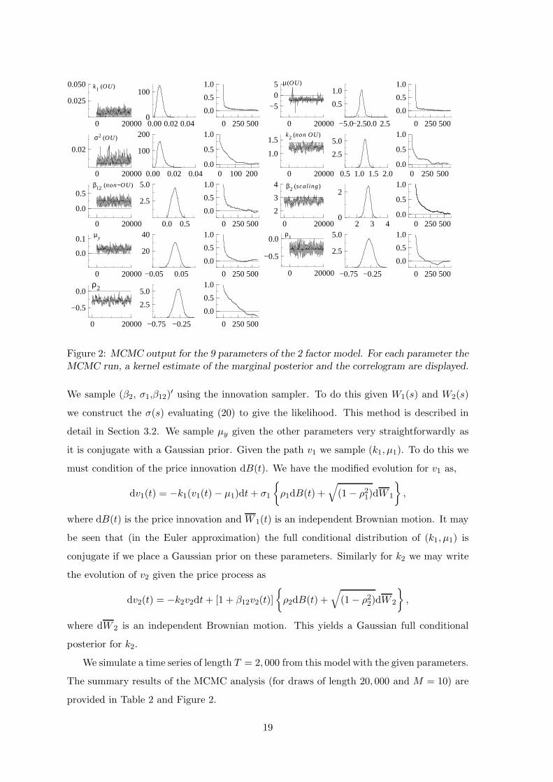
Figure 2: MCMC output for the 9 parameters of the 2 factor model. For each parameter the

MCMC run, a kernel estimate of the marginal posterior and the correlogram are displayed.

We sample (β2, σ1,β12)′ using the innovation sampler. To do this given W1(s) and W2(s)

we construct the σ(s) evaluating (20) to give the likelihood. This method is described in

detail in Section 3.2. We sample µy given the other parameters very straightforwardly as

it is conjugate with a Gaussian prior. Given the path v1 we sample (k1, µ1). To do this we

must condition of the price innovation dB(t). We have the modified evolution for v1 as,

dv1(t) = −k1(v1(t)− µ1)dt+ σ1

{ρ1dB(t) +

√(1− ρ21)dW 1

},

where dB(t) is the price innovation and W 1(t) is an independent Brownian motion. It may

be seen that (in the Euler approximation) the full conditional distribution of (k1, µ1) is

conjugate if we place a Gaussian prior on these parameters. Similarly for k2 we may write

the evolution of v2 given the price process as

dv2(t) = −k2v2dt+ [1 + β12v2(t)]

{ρ2dB(t) +

√(1− ρ22)dW 2

},

where dW 2 is an independent Brownian motion. This yields a Gaussian full conditional

posterior for k2.

We simulate a time series of length T = 2, 000 from this model with the given parameters.

The summary results of the MCMC analysis (for draws of length 20, 000 and M = 10) are

provided in Table 2 and Figure 2.

19

4.2 Univariate volatility models: S & P 500

In this section we estimate the volatility with leverage model of (1) to daily returns data

on the closing prices of the Standard and Poor’s 500 index from 5/5/1995 to 14/4/2003

(T = 2, 000) for a variety of common diffusive driven models. The price equation is again

given by (3) and we consider the three following forms for the volatility process σ2(t):

dσ2(t) = θ4σ2(t)

(θ5 − log σ2(t)

)dt+ θ3σ

2(t)dW (t), log-normal

dσ2(t) = θ4(θ5 − σ2(t)

)dt+ θ3σ(t)dW (t), CIR

dσ2(t) = θ4(θ5 − σ2(t)

)dt+ θ3σ

2(t)dW (t), GARCH diffusion.

The first model is the familiar (but reparameterised) OU log volatility model we have

examined in Sections 3.3 and 2.3. This has been proposed by Wiggins (1987), Chesney

and Scott (1989) and Scott (1991) for options pricing. The second model is a square root

process of Heston (1993). The third model is the diffusion limit of a GARCH(1,1) process

as shown by Nelson (1990). The marginal distributions of these stationary models for σ2

are log-Normal, Gamma and inverse-Gamma respectively. Throughout

Corr(B(t),W (t)) = ρ.

For our MCMC approach we sample the parameters following Section 3.1. The sampling

of the states is done following Section 2.2. We transform to the real line by using the Ito

transformation of each of the three state equations above and using the Euler scheme. We

now carry out inference on the parameters λ = (θ1, θ2, ρ)′ and ψ = (θ4, θ5)

′ and ω = θ3.

Again the priors and sampling strategies for the parameters are discussed in the Appendix.

We run 20, 000 iterations of the innovation MCMC algorithm, of Algorithm 3.2, using

the θ,W |Y parameterisation for M = 1, 4, 10 and 20. We sample, on average, 10 days of

the volatility diffusion at a time, regardless of M . The log-likelihood (estimated at the

mean of θ|y) is computed using particle filter methods, see Pitt and Shephard (1999b). The

correlograms from the MCMC output are shown in Figure 3 (for M = 10 for brevity). The

posterior kernel density estimates are given in Figure 4 for the parameters of the volatility

equation and Figure 5 for the return parameters (mean return, risk premium and leverage).

To calibrate these numbers, when we fit the Gaussian-GARCH(1,1) by maximum likelihood

(with the inclusion of the mean return and risk premium) the corresponding maximised

log-likelihood is −3, 074. Numerical summaries of the marginal posterior densities for each

parameter, including the inefficiency factors, are provided in Table 3 for M = 1, 4, 10 and

20.

20

Leverage is important as we find ρ to be highly negative in all cases. When the leverage

parameter ρ is constrained to 0 we find that θ1 and θ2 are different from 0 (results not

reported here) and the log-likelihoods evaluated at θ, the posterior mean of the parame-

ters, are −3, 040.2, −3, 059.3, −3, 037.3 for the SQRT, OU and GARCH diffusion models,

respectively. Notice these are much higher than the Gaussian-GARCH model mentioned

in the previous paragraph. When ρ is left unconstrained we see from Table 3 that both

parameters are close to 0 and that the reported log-likelihood value increases considerably

for each of the three models. Quantitatively there is a degree of robustness associated with

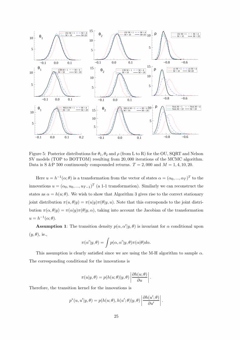
the estimation of ρ as we obtain similar results across models. We also see from Figure

4 that increasing M has little effect on the marginal posterior densities of the parameters

(θ3, θ4, θ5)′. However, the effect on the return parameters (Figure 5) is more substantial,

and the choice M = 1 is inadequate. Increasing M from 1 to 4 is sufficient for the pa-

rameters (θ1, θ2)′ whereas for ρ inferences based on M = 1 or 4 are different in the SQRT

and GARCH diffusion models from those made with M = 10 or 20. The reason that M

needs to be moderately large for ρ is due to the dependence on the Ito integral Zi in (4); in

contrast, for the case of σ2i the integrator is time. This effect was also seen in the results

for the simulated example of Section 3.3.

It can also be observed that as we increase the value of M from 1, ρ decreases quite

substantially (almost by one standard deviation) to less than −0.8 in each model. In

addition, the posterior standard deviation of θ6 falls as M increases. Further increases in

M (beyond 10) do not affect the results. In all cases the inefficiency factors, given in Table

3, are less than 100 and vary little with M . This again indicates that our methods are

invariant to M in terms of the efficiency factors. Thus the choice M = 10 is adequate in

this example. The resulting dimension of the discretised volatility path is 20, 000.

Whilst the differences between the three models, in terms of log-likelihood, are large

when leverage is not included, the differences disappear when leverage is included. When

leverage is included, the SQRT model for volatility appears to provide the best fit. The log

likelihoods of these models are all high relative to a competing GARCH(1, 1) model.

In this application we have demonstrated that the degree of augmentation is important

in obtaining correct inference. It is also apparent that our methodology does not suffer from

any degeneracy associated with augmentation which affects existing Bayesian methodology

for these problems. Our algorithm is efficient in an absolute sense, producing low integrated

autocorrelation times. It is also sufficiently general to enable comparison between competing

diffusion models for volatility.

21

CIR model: log lik (θ) = −2997.86

θ1 θ2 θ23M mean. st.dev INF(300) mean st.dev. INF(50) mean st.dev. INF(500)

1 0.0274 0.0348 18.7 0.0022 0.0301 14.3 0.0363 0.0088 86.8

4 -0.0115 0.0388 28.9 0.0305 0.0325 18.6 0.0388 0.0087 71.9

10 -0.0227 0.0384 17.1 0.0368 0.0320 14.1 0.0368 0.0076 68.6

20 -0.0277 0.0383 27.1 0.0392 0.0315 18.0 0.0377 0.0074 70.7

θ4 θ5 ρ

M mean st.dev. INF(50) mean st.dev. INF(50) mean st.dev. INF(500)

1 0.028 0.0079 33.0 1.43 0.213 5.8 -0.746 0.0515 55.1

4 0.030 0.0080 37.9 1.43 0.209 7.3 -0.802 0.0452 97.7

10 0.029 0.0075 22.3 1.45 0.196 8.2 -0.830 0.0371 66.0

20 0.029 0.0075 32.6 1.46 0.198 9.2 -0.835 0.0352 82.3

log OU model: log lik (θ) = −2999.44

θ1 θ2 θ23M mean st.dev. INF(300) mean st.dev. INF(50) mean st.dev. INF(500)

1 0.0313 0.0342 12.1 -0.0722 0.0280 2.53 0.0302 0.0060 32.0

4 0.0085 0.0344 14.3 0.0159 0.0292 9.89 0.0333 0.0068 60.2

10 0.0046 0.0344 10.9 0.0189 0.0295 7.79 0.0319 0.0068 16.3

20 0.0051 0.0358 13.6 0.0206 0.0297 8.65 0.0328 0.0070 54.8

θ4 θ5 ρ

M mean st.dev. INF(50) mean st.dev. INF(50) mean st.dev. INF(500)

1 0.024 0.0066 20.9 0.712 0.233 7.1 -0.774 0.0515 34.1

4 0.027 0.0071 27.7 0.709 0.216 7.8 -0.821 0.0392 51.8

10 0.026 0.0071 12.4 0.707 0.217 9.4 -0.824 0.0397 71.6

20 0.027 0.0072 31.5 0.718 0.214 7.0 -0.825 0.0365 67.8

Nelson model: log lik (θ) = −2999.54

θ1 θ2 θ23M mean st.dev. INF(300) mean st.dev. INF(50) mean st.dev. INF(500)

1 0.0538 0.0325 14.2 -0.0730 0.0287 2.42 0.0289 0.0063 44.3

4 0.0330 0.0331 17.4 -0.0041 0.0247 2.76 0.0313 0.0081 87.1

10 0.0271 0.0309 22.5 -0.0014 0.0236 3.67 0.0300 0.0059 30.6

20 0.0220 0.0317 19.3 0.0017 0.0235 4.52 0.0287 0.0061 56.3

θ4 θ5 ρ

M mean st.dev. INF(50) mean st.dev. INF(50) mean st.dev. INF(500)

1 0.0088 0.0054 15.5 2.96 2.24 4.10 -0.746 0.0541 47.1

4 0.0095 0.0057 22.7 2.93 2.33 6.18 -0.807 0.0499 51.5

10 0.0087 0.0054 18.3 3.06 2.27 2.72 -0.832 0.0430 68.0

20 0.0085 0.0054 23.5 3.09 2.32 7.13 -0.840 0.0391 59.6

Table 3: Posterior estimation results for the SQRT, OU, and Nelson SV models. 20, 000iterations used for MCMC algorithm. Data is S &P 500 continuously componded returns.T = 2 , 000 , M = 1, 4, 10 and 20. Log-likelihoods (at posterior means) estimated via theparticle filter.

22

0 50 100 150 200 250 300

0.0

0.5

1.0

θ3 CIR θ3 Nelson

θ3 OU

0 10 20 30 40 50

0.0

0.5

1.0 θ4 CIR θ4 Nelson

θ4 OU

0 100 200 300 400 500

0.0

0.5

1.0

θ5 CIR θ5 Nelson

θ5 OU

0 100 200 300 400 500

0.0

0.5

1.0θ1 CIR θ1 Nelson

θ1 OU

0 100 200 300 400 500

0.0

0.5

1.0 θ2 CIR θ2 Nelson

θ2 OU

0 100 200 300 400 500

0.0

0.5

1.0ρ CIR ρ Nelson

ρ OU

Figure 3: Correlograms for 6 parameters from the three SV models (CIR, log OU, Nelson)resulting from 20, 000 iterations of the MCMC algorithm. Data: S &P 500 continuouslycompounded returns with T = 2, 000 and M = 10.

5 Conclusion

This paper has provided a unified likelihood based approach for inference in diffusion driven

state space models. This is based on a effective proposal scheme for sampling subpaths of

the diffusive process and a reparameterisation of the model to overcome degeneracies in the

MCMC algorithm. This method is rather robust and can, in principle, work even in the

context of large dimensional diffusions or diffusions with many state variables. The analysis

we have described can be extended to deal with the problem of filtering, by applying the

approach of Pitt and Shephard (1999b), and to the problem of model choice by using the

method of Chib (1995) and Chib and Jeliazkov (2001) to estimate the marginal likelihood

of the data under each model. Finally, the various empirical studies show that the approach

detailed in this paper has considerable promise for applied work.

6 Acknowledgments

Neil Shephard’s research is supported by the ESRC through the grant “High frequency

financial econometrics based upon power variation.” The code for the calculations in the

23

0.000 0.025 0.050

25

50θ3

2 OU M = 1 M = 10

M = 4 M = 20

−1 0 1

1

2θ4

OU M = 1 M = 10

M = 4 M = 20

0.025 0.050 0.075

25

50

75θ5

OU M = 1 M = 10

M = 4 M = 20

0.000 0.025 0.050

20

40

60

θ32

θ32

θ4

CIR M = 1 M = 10

M = 4 M = 20

1 2 3

1

2 CIR M = 1 M = 10

M = 4 M = 20

0.025 0.050 0.075

25

50θ5

CIR M = 1 M = 10

M = 4 M = 20

0.00 0.02 0.04

25

50

75NELS M = 1 M = 10

M = 4 M = 20

0 5 10 15

0.2

0.4θ4 NELS M = 1 M = 10

M = 4 M = 20

0.025 0.050 0.075

25

50

75

θ5

NELS M = 1 M = 10

M = 4 M = 20

Figure 4: Posterior distributions for θ23, θ4 and θ5 (from L to R) for the OU, SQRT andNelson SV models (TOP to BOTTOM) resulting from 20, 000 iterations of the MCMCalgorithm. Data is S &P 500 continuously compounded returns. T = 2, 000 and M =1, 4, 10, 20.

paper was written in the Ox language of Doornik (2001).

7 Appendix

7.1 Proof of innovation sampler

We will state the algorithm in a general manner for the innovation algorithm applied to a

general finite dimensional problem. The validity of the method is not obvious as we do not

have a Gibbs-type (Metropolis within Gibbs) method in the innovations. The innovation

algorithm is defined as follows:

Innovation Algorithm :

1. Draw α′ by M-H conditional on (y, θ) from the conditional density π(α|y, θ). Let theM-H transition kernel be p(α,α′|y, θ)

2. Set u′ = h−1(α′; θ)

3. Draw θ′ from the full conditional density π(θ′|y, u′).

24

−0.8 −0.6

5

10 ρ OU M = 1 M = 10

M = 4 M = 20

−0.8 −0.6

5

10

15ρ cir M = 1

M = 10 cir M = 4 M=20

−0.8 −0.6

5

10 ρ Nels M = 1 Nels M = 10

Nels M = 4 M = 20

−0.1 0.0 0.1

5

10 θ1

OU M = 1 M = 10

M = 4 M=20

−0.1 0.0 0.1

5

10

15θ2

OU M = 1 M = 10

M = 4 M=20

−0.1 0.0 0.1

5

10θ1

θ1

CIR M = 1 M = 10

M = 4 M = 20

−0.1 0.0 0.1

5

10

15 θ2

θ2

CIR M = 1 M = 10

M = 4 M = 20

−0.1 0.0 0.1 0.2

5

10

NELS M = 1 M = 10

M = 4 M = 20

−0.1 0.0 0.1

5

10

15NELS M = 1 M = 10

M = 4 M = 20

Figure 5: Posterior distributions for θ1, θ2 and ρ (from L to R) for the OU, SQRT and NelsonSV models (TOP to BOTTOM) resulting from 20, 000 iterations of the MCMC algorithm.Data is S &P 500 continuously compounded returns. T = 2, 000 and M = 1, 4, 10, 20.

Here u = h−1(α; θ) is a transformation from the vector of states α = (α0, ..., αT )T to the

innovations u = (α0, u0, ..., uT−1)T (a 1-1 transformation). Similarly we can reconstruct the

states as α = h(u; θ). We wish to show that Algorithm 3 gives rise to the correct stationary

joint distribution π(u, θ|y) = π(u|y)π(θ|y, u). Note that this corresponds to the joint distri-

bution π(α, θ|y) = π(α|y)π(θ|y, α), taking into account the Jacobian of the transformation

u = h−1(α; θ).

Assumption 1: The transition density p(α,α′|y, θ) is invariant for α conditional upon

(y, θ), ie.,

π(α′|y, θ) =∫p(α,α′|y, θ)π(α|θ)dα.

This assumption is clearly satisfied since we are using the M-H algorithm to sample α.

The corresponding conditional for the innovations is

π(u|y, θ) = p(h(u; θ)|y, θ)∣∣∣∣∂h(u; θ)

∂u

∣∣∣∣ .

Therefore, the transition kernel for the innovations is

p∗(u, u′|y, θ) = p(h(u; θ), h(u′; θ)|y, θ)∣∣∣∣∂h(u′; θ)

∂u′

∣∣∣∣ .

25

Assume for now that θ can be sampled from π(θ|y, u) directly. This means that the transi-

tion kernel of the parameters and innovations is,

p∗({u, θ} → {u′, θ′}|y) = p∗(u, u′|y, θ)π(θ′|y, u) (21)

We show that the latter kernel is invariant which means that Algorithm 3 gives the correct

stationary distribution.

Proposition 3 The transition kernel p∗({u, θ} → {u′, θ′}|y) is invariant, ie.,

π(u′, θ′|y) =∫p∗({u, θ} → {u′, θ′}|y)π(u, θ|y)dudθ (22)

Proof. Taking the right hand side,

∫p∗({u, θ} → {u′, θ′}|y)π(u, θ|y)dudθ

=

∫p∗(u, u′|y, θ)π(θ′|y, u′)π(u, θ|y)dudθ

= π(θ′|y, u′)∫

θ

{∫

u

p∗(u, u′|y, θ)π(u|y, θ)du}π(θ|y)dθ

Now the inner integral is

∫

u

p∗(u, u′|y, θ)π(u|y, θ)du

=

∫

u′

p(h(u; θ), h(u′; θ)|y, θ)∣∣∣∣∂h(u′; θ)

∂u′

∣∣∣∣ p(h(u; θ)|y, θ)∣∣∣∣∂h(u; θ)

∂u

∣∣∣∣ du

=

∣∣∣∣∂h(u′; θ)

∂u′

∣∣∣∣∫

α

p(α,α′|y, θ)π(α|θ)dα.

By assumption 1, this becomes

∣∣∣∣∂h(u′; θ)

∂u′

∣∣∣∣π(α′|y, θ) = π(u′|y, θ).

So the whole LHS expression becomes,

= π(θ′|y, u′)∫

θ

π(u′|y, θ)π(θ|y)dθ

= π(θ′|y, u′)π(u′|y) as required.

We now detail the prior for θ and the method for sampling parameters. In this section

we shall focus on the models of Section 4. We will examine the SQRT and GARCH models

in particular detail. The overview of the methods is given in Section 3.1.

26

7.2 Parameter priors and sampling

This section describes the priors for the parameters and the MCMC method in detail used

for the stochastic volatility model of Section 3.3. We deal firstly with the measurement

parameters λ′ = (θ1, θ2, ρ)′, then the drift and volatility parameters which are denoted by

ψ′ = (θ4, θ5)′ and ω = θ3 respectively.

7.2.1 Measurement parameters

The measurement parameters λ′ = (θ1, θ2, ρ)′ from Sections 3.3 and 4 are common across the

different volatility models. These comprise of the mean return, the risk premium parameter

and the leverage parameter respectively. For unit time separation of the returns Yi =

P (i)− P (i− 1), we obtain,

Yi|σ2i , Zi ∼ N(θ1 + θ2σ

2i + ρZi,

(1− ρ2

)σ2i),

where the sufficient integrated quantities are given, from the Euler approximation, by (18).

As we are conditioning upon ψ′ = (θ4, θ5)′ and ω = θ3 these sufficient quantities σ2i and

Zi are fixed for this point in the algorithm. We now use the following representations

σ2 = (σ21 , . . . , σ2T )

′, Z = (Z1, . . . , ZT ) and Y = (Y1, . . . , YT )′. Sampling of λ′ = (θ1, θ2, ρ)

′

consists of the two following Metropolis-within Gibbs steps:

1. Sample from

π(θ1, θ2|σ2, Z, Y ; ρ) ∝ f(Y |σ2, Z; θ1, θ2, ρ)π(θ1, θ2).

2. Sample from

π(ρ|σ2, Z, Y ; θ1, θ2) ∝ f(Y |σ2, Z; θ1, θ2, ρ)π(ρ).

We take a standard, relatively uninformative, conjugate prior (θ1, θ2)′ ∼ N2(0, 1000 ×

I2).Step (1) is therefore a straightforward Gibbs step as, conditionally, we have a Gaussian

posterior for (θ1, θ2)′. Step (2) is performed using a t-distribution proposal (formed using a

Laplace approximation) for φ = log ((1 + ρ)/(1 − ρ)) .We also take a vague prior on φ whish

is N(0, 1000), ensuring that the leverage parameter ρ ∈ (−1, 1) . This proposal is accepted,

or rejected, using a Metropolis criterion. In practice we find that the acceptance probability

from this step is over 97%.

7.2.2 Drift and volatility parameters

For all three volatility models of Sections 3.3 and 4 we have the three parameters ψ′ =

(θ3, θ4, θ5)′. We deal with the three models for volatility given in Remark 3 of Section 4.

The volatility parameter update consists of:

27

1. Sample from

π(θ4, θ5|Y, α; θ3) ∝ f(Y |α; θ3, λ)f(α|θ3, θ4, θ5)π(θ4, θ5).

2. Sample from

π(θ3|Y, α;λ, θ4, θ5) ∝ f(Y |α; θ3, λ)f(α|θ3, θ4, θ5)π(θ3).

For step (1) the dependence upon the observations is because the integrals Zi depend

upon the innovations dW (u). These will change as the parameters θ4 and θ5 vary. However,

the contribution is not great and we propose using the density

g(θ4, θ5|Y, α; θ3) ∝ f(α|θ3, θ4, θ5)π(θ4, θ5),

correcting for the missing term f(Y |α; θ3, λ) in the Metropolis algorithm. In each of the

three models for α we now have we have a linear form in each case upon reparameterising

as β0 = θ4θ5 and β1 = −θ4. For instance, in the first model, the OU model of Section 4, we

obtain form the Euler discretisation,

αj+1 − αj =1

M

(β0θ3

+β1θ3αj −

θ32

)+

1√Muj ,

where uj is a standard Gaussian random variate. Upon rearranging we obtain,

zj = β0 + β1αj +√Mθ3uj ,

where zj = Mθ3(αj+1 − αj) + θ23/2. The model is now in linear form, given θ3. Similar

approaches are used for the CIR and GARCH diffusion models. This means that with we

may easily sample from π(β0, β1|α; θ3), transforming back to the parameters θ4, θ5. We

incorporate Gaussian priors on θ4, θ5, as we find these more interpretable and obtain a

Metropolis acceptance rate which is very high (greater than 98% typically).

These parameters have slightly different interpretations across the three models. How-

ever θ4 determines the persistence in each case and θ5 determines the mean reversion. For

θ4 we choose the truncated Gaussian distribution prior

θ4 ∼ NT>0(0.03, 0.22).

For the log OU model there is no restriction on the mean reversion θ5 parameter and we

take θ5 ∼ N(0, 102). For the SQRT and Nelson models we have the unconditional mean has

to be positive and so we take the truncated prior

θ5 ∼ NT>0(0, 102).

28

The density of step (2) is more complicated. We have

π(θ3|Y, α;λ, θ4, θ5) ∝ f(Y |α; θ3, λ)p(α|θ3, θ4, θ5)π(θ3).

Here we have take account of the measurement density f(Y |α; θ3, λ) as it is very informative.

Both the integrals σ2i and Zi vary substantially as we alter θ3. We use a Laplace approxi-

mation (centred at the mode) of π(θ3|Y, α;λ, θ4, θ5) but using a t-distribution rather than

a Gaussian density. This gives an extremely high acceptance probability in the resulting

Metropolis algorithm. We have a standard, inverse gamma, prior for θ23 ∼ Iga (ν; ν × 0.03)

where we set ν = 2.

7.3 Algorithm for partially observed diffusions

We now turn to an analysis of partially observed diffusions. This allows the consideration of

multivariate diffusions allowing flexibility in the overall simulation scheme, see Section 4.1.

We shall assume the multivariate diffusion evolves as described in Section 1, see Equation

2. However, now the observed data is given by

y(τi) = Zα(τi), i = 1, ..., T,

where Z is a non-random k×d matrix. In this case the diffusion includes the observations as

Z is a selection matrix. The key difference in approach for dealing with this (non-Markov)

situation is that now it is not particularly helpful to consider blocks defined in terms of the

latent α+i between yi and yi+1. Instead it is necessary to work with the entire α+ in terms

of the natural complete ordering on the Euler scale,

α+ = (α0, α1, ..., αM(T−1))′, yi = ZαM(i−1), i = 1, . . . , T. (23)

To sample this very high-dimensional latent vector from its distribution conditioned on the

observed data and the parameters, we subdivide α+ randomly into B blocks

α+ = (α+(1), α+(2), ..., α+(B))′.

Corresponding to these blocks we write

y = (y+(1), y+(2), ..., y+(B))′,

the real observations which fall within these blocks. Each block α+(l) may contain more or

less thanM vectors of the diffusion and so y+(l) could include single vectors of observations,

multiple observations or could be the null set. We randomly determine the positions of the

blocks. The task then reduces, for each of the blocks, to sampling the block given the first

29

element of the next block, the last element of the preceding block and the observations

within the block. That is for each block l we simulate from

f(α+(l)|α+(l−1)Nl−1

, α+(l+1)1 , y+(l)),

where Nl is the number of elements in this block. The fact that we condition only on

α+(l−1)Nl−1

, α+(l+1)1 and y(l) is due to the Markovian nature of the diffusion.

In order to focus on the main idea we suppress the superscript l and write α∗′ =

(α′1, ..., α

′N−1), the block under consideration, and equivalently think about sampling from

α∗|α0, αN , y+.

Clearly if y+ is the null set, then we can update samples from this distribution by using

the bridge sampler described in Section 2.2. Hence in that case no new issues arise. Before

considering the case of multiple observations it is helpful to think about y+ containing only

a single observation, on the Euler timing scale, within this block, represented by yk. This

notation means this observation corresponds to yk = Zαk, where 0 < k < N . In this case

we have to sample from the full conditional density

f(α∗|α0, αN , yk) = I(yk = Zαk)

N∏

j=1

f(αj |αj−1)

/f(yk, αN |α0). (24)

As in Section 2.2, the normalizing term f(αN , yk|α0) is unknown to us. However we can

evaluate the numerator of (24), allowing the use of the Metropolis method.

In theory this can be rewritten as

f(α∗|α0, αN , yk) =N−1∏

j=1

f(αj|αj−1, yk, αN ) (25)

=k∏

j=1

f(αj|αj−1, yk, αN )N−1∏

j=k+1

f(αj |αj−1, αN ). (26)

The αj |αj−1, αN terms in (26) are essentially the expressions which appeared in Section

2.2, see (13). We therefore know how to form approximations to the terms f(αj |αj−1, αN ).

Hence the only remaining issue is how to approximate f(αj |αj−1, yk, αN ).

We parallel the approach of Durham and Gallant (2002) extending this to partial obser-

vations. Considering the first product in (26) for j < k < N , we consider the approximate

system,

f(αk|αj) = N(αk|αj + µ(αj−1)δ(k − j),Σ(αj−1)δ(k − j)),

f(αN |αk) = N(αN |αk + µ(αj−1)δ(N − k),Σ(αj−1)δ(N − k)),yk = Zαk.

(27)

30

Then,

αj|αj−1, yk, αN ∼ Nd

(m†

j, V†j

), (28)

where the mean and covariance are given in the following Proposition (without proof).

Proposition 4 Writing Σj−1 = Σ(αj−1) and

mj =αN − αj−1

(N − j + 1), vj = δ

(N − j)

(N − j + 1),

and

cj = 1− (k − j)

N − j, m∗

j =(k − j)

N − jαN , v∗j = δ

(k − j) (N − k)

(N − j).

Then αj |αj−1, yk, αN ∼ Nd

(m†

j , V†j

)where

(V †j

)−1= v−1

j Σ−1j−1 +

c2jv∗jZ ′(ZΣj−1Z

′)−1

Z

and (V †j

)−1m†

j = v−1j Σ−1

j−1 (αj−1 +mj) +cjv∗jZ ′(ZΣj−1Z

′)−1 (

yk − Zm∗j

).

The proposal on the entire block is thus

q(α1, ..., αN−1|α0, yk, αN ) =k∏

j=1

q(αj |αj−1, yk, αN )N−1∏

j=k+1

q(αj |αj−1, αN ), (29)

where q(αj |αj−1, αN ) has moments, see Section 2.2, which are αj−1 +mj and vjΣj−1 re-

spectively, similar to Durham and Gallant (2002), and

q(αj |αj−1, yk, αN ) = Nd

(m†

j, V†j

),

defined above.

We can now propose from q(α1, ..., αN−1|α0, yk, αN ) and compare with the true density

given by (24) in a Metropolis algorithm. This is a direct generalisation of the algorithm in

Section 2.2. We can see that if there are no observations within the block then the true

density given by (24) reduces to that of Section 2.2. Similarly, we attain the same setup if

we observe αk exactly, that is when Z = Id. The computational complexity of the method,

which involves simulating from (29) and evaluating the Metropolis acceptance probability,

is of order N − 1, as in Section 2.2.

We shall use this strategy for formulating our proposal even when there are an arbitrary

number of measurements in the block under consideration. To see the general approach it

is sufficient to consider the case of two observations within the block, y+ = (yk, yl), where

0 < k < l < N . The generalisation to many observations is immediate and computationally

31

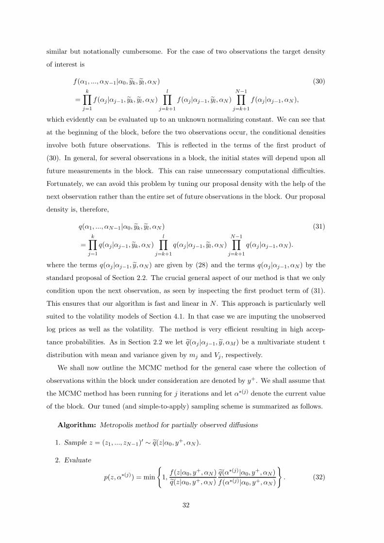
similar but notationally cumbersome. For the case of two observations the target density

of interest is

f(α1, ..., αN−1|α0, yk, yl, αN ) (30)

=

k∏

j=1

f(αj |αj−1, yk, yl, αN )

l∏

j=k+1

f(αj|αj−1, yl, αN )

N−1∏

j=k+1

f(αj|αj−1, αN ),

which evidently can be evaluated up to an unknown normalizing constant. We can see that

at the beginning of the block, before the two observations occur, the conditional densities

involve both future observations. This is reflected in the terms of the first product of

(30). In general, for several observations in a block, the initial states will depend upon all

future measurements in the block. This can raise unnecessary computational difficulties.

Fortunately, we can avoid this problem by tuning our proposal density with the help of the

next observation rather than the entire set of future observations in the block. Our proposal

density is, therefore,

q(α1, ..., αN−1|α0, yk, yl, αN ) (31)

=k∏

j=1

q(αj|αj−1, yk, αN )l∏

j=k+1

q(αj|αj−1, yl, αN )N−1∏

j=k+1

q(αj |αj−1, αN ).

where the terms q(αj |αj−1, y, αN ) are given by (28) and the terms q(αj|αj−1, αN ) by the

standard proposal of Section 2.2. The crucial general aspect of our method is that we only

condition upon the next observation, as seen by inspecting the first product term of (31).

This ensures that our algorithm is fast and linear in N . This approach is particularly well

suited to the volatility models of Section 4.1. In that case we are imputing the unobserved

log prices as well as the volatility. The method is very efficient resulting in high accep-

tance probabilities. As in Section 2.2 we let q(αj |αj−1, y, αM ) be a multivariate student t

distribution with mean and variance given by mj and Vj , respectively.

We shall now outline the MCMC method for the general case where the collection of

observations within the block under consideration are denoted by y+. We shall assume that

the MCMC method has been running for j iterations and let α∗(j) denote the current value

of the block. Our tuned (and simple-to-apply) sampling scheme is summarized as follows.

Algorithm: Metropolis method for partially observed diffusions

1. Sample z = (z1, ..., zN−1)′ ∼ q(z|α0, y

+, αN ).

2. Evaluate

p(z, α∗(j)) = min

{1,f(z|α0, y

+, αN )

q(z|α0, y+, αN )

q(α∗(j)|α0, y+, αN )

f(α∗(j)|α0, y+, αN )

}. (32)

32

3. With probability p(z, α∗(j)), set α∗(j+1) = z; otherwise set α∗(j+1) = α∗(j).

References

Ait-Sahalia, Y. (2002). Maximum likelihood estimation of discretely sampled diffusions:a closed-form approach. Econometrica 70, 223–262.

Ait-Sahalia, Y. (2003). Closed-form likelihood expansions for multivariate diffusions. Un-published paper: Department of Economics, Princeton University.

Aıt-Sahalia, Y., L. P. Hansen, and J. Scheinkman (2004). Discretely sampled diffusions.In Y. Aıt-Sahalia and L. P. Hansen (Eds.), Handbook of Financial Econometrics.Amsterdam: North Holland.

Andersen, T. G., L. Benzoni, and J. Lund (2002). An empirical investigation ofcontinuous-time equity return models. Journal of Finance 57, 1239–1284.

Andersen, T. G., T. Bollerslev, and F. X. Diebold (2007). Roughing it up: Includingjump components in the measurement, modeling and forecasting of return volatility.The Review of Economics and Statistics 89 (4), 701–720.

Beskos, A., O. Papaspiliopoulos, and G. Roberts (2009). Monte Carlo maximum like-lihood estimation for discretely observed diffusion processes. The Annals of Statis-tics 37 (1), 223–245.

Beskos, A., O. Papaspiliopoulos, G. O. Roberts, and P. Fearnhead (2006). Exact andcomputationally efficient likelihood-based estimation for discretely observed diffusionprocesses (with discussion). Journal of the Royal Statistical Society: Series B 68 (3),333–382.

Beskos, A. and G. Roberts (2005). Exact simulation of diffusions. Annals of AppliedProbability 15 (4), 2422–2444.

Bibby, B. M., M. Jacobsen, and M. Sørensen (2004). Estimating functions for discretelysamples diffusion-type models. In Y. Aıt-Sahalia and L. P. Hansen (Eds.), Handbookof Financial Econometrics. Amsterdam: North Holland. Forthcoming.

Brandt, M. W. and P. Santa-Clara (2002). Simulated likelihood estimation of diffusionswith an application to exchange rates dynamics in incomplete markets. Journal ofFinancial Economics 63, 161–210.

Chernov, M., A. R. Gallant, E. Ghysels, and G. Tauchen (2003). Alternative models ofstock price dynamics. Journal of Econometrics 116, 225–257.

Chesney, M. and L. O. Scott (1989). Pricing European options: a comparison of the mod-ified Black-Scholes model and a random variance model. J. Financial and QualitativeAnalysis 24, 267–84.

Chib, S. (1995). Marginal likelihood from the Gibbs output. Journal of the AmericanStatistical Association 90, 1313–21.

Chib, S. (2001). Markov chain Monte Carlo methods: computation and inference. In J. J.Heckman and E. Leamer (Eds.), Handbook of Econometrics, Volume 5, pp. 3569–3649.Amsterdam: North-Holland.

Chib, S. and E. Greenberg (1995). Understanding the Metropolis-Hastings algorithm.The American Statistican 49, 327–35.

33

Chib, S. and I. Jeliazkov (2001). Marginal likelihood from the Metropolis-Hastings output.Journal of the American Statistical Association 96, 270–281.

Chib, S. and N. Shephard (2002). Comment on ‘Numerical techniques for maximumlikelihood estimation of continuous-time diffusion processes,’ by Durham and Gallant.Journal of Business and Economic Statistics 20, 325–327.

Cox, D. R. (1955). Some statistical models connected to a series of events (with discus-sion). Journal of the Royal Statistical Society, Series B 17, 129–64.

Doornik, J. A. (2001). Ox: Object Oriented Matrix Programming, 3.0. London: Timber-lake Consultants Press.

Duffie, D. and K. Singleton (1999). Modeling term structures of defaultable bonds. Reviewof Financial Studies 12, 687–720.

Durbin, J. and S. J. Koopman (2001). Time Series Analysis by State Space Methods.Oxford: Oxford University Press.

Durham, G. (2003). Likelihood-based specification analysis of continuous-time models ofthe short-term interest rate. Journal of Financial Economics 70, 463–487.

Durham, G. and A. R. Gallant (2002). Numerical techniques for maximum likelihood es-timation of continuous-time diffusion processes (with discussion). Journal of Businessand Economic Statistics 20, 297–338.

Elerian, O. (1999). Simulation estimation of continuous-time models with applications tofinance. Unpublished D.Phil. thesis, Nuffield College, Oxford.

Elerian, O., S. Chib, and N. Shephard (2001). Likelihood inference for discretely observednon-linear diffusions. Econometrica 69, 959–993.

Eraker, B. (2001). Markov chain Monte Carlo analysis of diffusion models with applicationto finance. Journal of Business and Economic Statistics 19, 177–191.

Eraker, B., M. Johannes, and N. G. Polson (2003). The impact of jumps in returns andvolatility. Journal of Finance 53, 1269–1300.

Gallant, A. R. and G. Tauchen (1996). Which moments to match. Econometric Theory 12,657–81.

Gallant, A. R. and G. Tauchen (2004). Simulated score methods and indirect inferencefor continuous-time models. In Y. Ait-Sahalia and L. P. Hansen (Eds.), Handbook ofFinancial Econometrics. Amsterdam: North Holland.

Geweke, J. (1989). Bayesian inference in econometric models using Monte Carlo integra-tion. Econometrica 57, 1317–39.

Ghysels, E., A. C. Harvey, and E. Renault (1996). Stochastic volatility. In C. R. Raoand G. S. Maddala (Eds.), Statistical Methods in Finance, pp. 119–191. Amsterdam:North-Holland.

Gourieroux, C., A. Monfort, and E. Renault (1993). Indirect inference. Journal of AppliedEconometrics 8, S85–S118.

Harvey, A. C. (1989). Forecasting, Structural Time Series Models and the Kalman Filter.Cambridge: Cambridge University Press.

Harvey, A. C. and S. J. Koopman (2000). Signal extraction and the formulation of un-observed components models. Econometrics Journal 3, 84–107.

Harvey, A. C. and J. H. Stock (1985). The estimation of higher order continuous timeautoregressive models. Econometric Theory 1, 97–112.

34

Harvey, A. C. and J. H. Stock (1988). Continuous time autoregressive models with com-mon stochastic trends. J. Economic Dynamics and Control 12, 365–84.

Heston, S. L. (1993). A closed-form solution for options with stochastic volatility, withapplications to bond and currency options. Review of Financial Studies 6, 327–343.

Huang, X. and G. Tauchen (2005). The relative contribution of jumps to total pricevariation. Journal of Financial Econometrics 3, 456–499.

Hurn, A., K. A. Lindsay, and V. L. Martin (2003). On the efficacy of simulated maximumlikelihood for estimating the parameters of stochastic differential equations. Journalof Time Series Analysis 24, 45–63.

Jacod, J. and P. Protter (1998). Asymptotic error distributions for the Euler method forstochastic differential equations. Annals of Probability 26, 267–307.

Jones, R. H. (1984). Fitting multivariate models to unequally spaced data. In E. Parzen(Ed.), Time Series Analysis of Irregularly Observed Data, Number 25 in Lecture Notesin Statistics, pp. 158–188. New York: Springer-Verlag.

Kalogeropoulos, K. (2007). Likelihood-based inference for a class of multivariate diffusionswith unobserved paths. Journal of Statistical Planning and Inference 137 (10), 3092–3102.

Kalogeropoulos, K., G. Roberts, and P. Dellaportas (2010). Inference for stochasticvolatility models using time change transformations. The Annals of Statistics 38 (2),784–807.

Kim, S., N. Shephard, and S. Chib (1998). Stochastic volatility: likelihood inference andcomparison with ARCH models. Review of Economic Studies 65, 361–393.

Kloeden, P. E. and E. Platen (1992). Numerical Solutions to Stochastic Differential Equa-tions. New York: Springer.

Lando, D. (1998). On Cox processes and credt risk securities. Review of DerivativesResearch 2, 99–120.

Nelson, D. B. (1990). Stationarity and persistence in the GARCH(1,1) model. Economet-ric Theory 6, 318–334.

Nicolau, J. (2002). A new technique for simulating the likelihood of stochastic differentialequations. Econometrics Journal 5, 91–103.

Øksendal, B. (1998). Stochastic Differential Equations. An Introduction with FinancialApplications (5 ed.). Berlin: Springer.

Pedersen, A. R. (1995). A new approach to maximum likelihood estimation for stochasticdifferential equations on discrete observations. Scandinavian Journal of Statistics 27,55–71.

Pitt, M. K. and N. Shephard (1999a). Analytic convergence rates and parameterisationissues for the Gibbs sampler applied to state space models. Journal of Time SeriesAnalysis 21, 63–85.

Pitt, M. K. and N. Shephard (1999b). Filtering via simulation: auxiliary particle filter.Journal of the American Statistical Association 94, 590–599.

Revuz, D. and M. Yor (1999). Continuous Martingales and Brownian motion (3 ed.).Heidelberg: Springer-Verlag.

Roberts, G. O. and O. Stramer (2001). On inference for nonlinear diffusion models usingthe Hastings-Metropolis algorithms. Biometrika 88, 603–621.

35

Scott, L. (1991). Random-variance option pricing. Advances in Future and Options Re-search 5, 113–135.

Shephard, N. (2005). Stochastic Volatility: Selected Readings. Oxford: Oxford UniversityPress.

Smith, A. A. (1993). Estimating nonlinear time series models using simulated vectorautoregressions. Journal of Applied Econometrics 8, S63–S84.

Wecker, W. E. and C. F. Ansley (1983). The signal extraction approach to nonlinearregression and spline smoothing. Journal of the American Statistical Association 78,81–89.

West, M. and J. Harrison (1997). Bayesian Forecasting and Dynamic Models (2 ed.). NewYork: Springer-Verlag.

Wiggins, J. B. (1987). Option values under stochastic volatilities. Journal of FinancialEconomics 19, 351–372.

36