limit analysis for shallow foundations and

Limit Analysis for Shallow Foundations andElastoplasticity Modeling

By

Felipe Cortés González

Advisor

Pr. Arcesio Lizcano Peláez Ph.D.

Universidad de los Andes

Faculty of Engineering

Department of Civil and Environmental Engineering

2009

Contents

1 Bearing Capacity 31.1 Introduction . . . . . . . . . . . . . . . . . . . . . . . . . . . . . . . . . . . . . . . . . . . 3

1.2 Bearing Capacity Analysis . . . . . . . . . . . . . . . . . . . . . . . . . . . . . . . . . . . 4

1.3 Limit Analysis . . . . . . . . . . . . . . . . . . . . . . . . . . . . . . . . . . . . . . . . . 6

1.3.1 Introduction . . . . . . . . . . . . . . . . . . . . . . . . . . . . . . . . . . . . . . . 6

1.3.2 Upper Bound Theorem: Undrained Analysis . . . . . . . . . . . . . . . . . . . . . 7

1.3.3 Lower Bound Theorem: Undrained Analysis . . . . . . . . . . . . . . . . . . . . . 12

1.3.4 Upper Bound Theorem: Drained Analysis . . . . . . . . . . . . . . . . . . . . . . . 17

1.3.5 Lower Bound Theorem: Drained Analysis . . . . . . . . . . . . . . . . . . . . . . . 21

1.3.6 Weight and Cohesion Influence on Soils . . . . . . . . . . . . . . . . . . . . . . . . 27

1.4 Formulating Bearing Capacity Equations . . . . . . . . . . . . . . . . . . . . . . . . . . . . 29

1.5 Special Considerations . . . . . . . . . . . . . . . . . . . . . . . . . . . . . . . . . . . . . 33

1.5.1 Influence of Foundation Shape-Depth and Footings under Inclined Loadings . . . . 33

1.5.2 Load Eccentricity . . . . . . . . . . . . . . . . . . . . . . . . . . . . . . . . . . . . 35

1.5.3 Bearing Capacity of Footings on Slopes . . . . . . . . . . . . . . . . . . . . . . . . 38

2 Constitutive Modeling in Soil Mechanics 412.1 Introduction . . . . . . . . . . . . . . . . . . . . . . . . . . . . . . . . . . . . . . . . . . . 41

2.2 Description . . . . . . . . . . . . . . . . . . . . . . . . . . . . . . . . . . . . . . . . . . . 42

2.3 Implementation . . . . . . . . . . . . . . . . . . . . . . . . . . . . . . . . . . . . . . . . . 42

3 Elasticity 433.1 Introduction . . . . . . . . . . . . . . . . . . . . . . . . . . . . . . . . . . . . . . . . . . . 43

3.2 Analyzing the Constitutive Equation . . . . . . . . . . . . . . . . . . . . . . . . . . . . . . 44

3.3 Model Parameters . . . . . . . . . . . . . . . . . . . . . . . . . . . . . . . . . . . . . . . . 47

4 Elastoplasticity 514.1 Introduction . . . . . . . . . . . . . . . . . . . . . . . . . . . . . . . . . . . . . . . . . . . 51

4.2 Yielding Criterion . . . . . . . . . . . . . . . . . . . . . . . . . . . . . . . . . . . . . . . . 52

4.3 Strains . . . . . . . . . . . . . . . . . . . . . . . . . . . . . . . . . . . . . . . . . . . . . . 53

i

CONTENTS ICIV 200522909

4.3.1 Elastic Strains . . . . . . . . . . . . . . . . . . . . . . . . . . . . . . . . . . . . . 54

4.3.2 Plastic Strains . . . . . . . . . . . . . . . . . . . . . . . . . . . . . . . . . . . . . . 58

4.4 Plastic Potential . . . . . . . . . . . . . . . . . . . . . . . . . . . . . . . . . . . . . . . . . 59

4.5 Hardening Law . . . . . . . . . . . . . . . . . . . . . . . . . . . . . . . . . . . . . . . . . 60

4.6 Flow Rule . . . . . . . . . . . . . . . . . . . . . . . . . . . . . . . . . . . . . . . . . . . . 62

4.7 Stiffness Modulus . . . . . . . . . . . . . . . . . . . . . . . . . . . . . . . . . . . . . . . . 63

5 Cam-Clay 645.1 Introduction . . . . . . . . . . . . . . . . . . . . . . . . . . . . . . . . . . . . . . . . . . . 64

5.2 Critical State Theory . . . . . . . . . . . . . . . . . . . . . . . . . . . . . . . . . . . . . . 65

5.3 Parameters . . . . . . . . . . . . . . . . . . . . . . . . . . . . . . . . . . . . . . . . . . . . 66

5.4 Yielding Surface Evolution (Flow Rule) . . . . . . . . . . . . . . . . . . . . . . . . . . . . 66

5.5 Hardening Rule . . . . . . . . . . . . . . . . . . . . . . . . . . . . . . . . . . . . . . . . . 68

5.6 Consolidation . . . . . . . . . . . . . . . . . . . . . . . . . . . . . . . . . . . . . . . . . . 68

6 Appendix 716.1 MATLAB Algorithm (Drained Test) . . . . . . . . . . . . . . . . . . . . . . . . . . . . . . 71

ii

List of Figures

1.1 Plastic Analysis . . . . . . . . . . . . . . . . . . . . . . . . . . . . . . . . . . . . . . . . . 4

1.2 Bearing Capacity Analysis (Shear Zones) . . . . . . . . . . . . . . . . . . . . . . . . . . . 5

1.3 Slip Circle Mechanism . . . . . . . . . . . . . . . . . . . . . . . . . . . . . . . . . . . . . 7

1.4 Slip Circle Mechanism Above Surface Level . . . . . . . . . . . . . . . . . . . . . . . . . . 8

1.5 Minimum Safety Plot . . . . . . . . . . . . . . . . . . . . . . . . . . . . . . . . . . . . . . 10

1.6 Rigid Blocks Mechanism . . . . . . . . . . . . . . . . . . . . . . . . . . . . . . . . . . . . 11

1.7 Collapse Mechanism (Shear Fan) . . . . . . . . . . . . . . . . . . . . . . . . . . . . . . . . 12

1.8 Stress Field (One Discontinuity) . . . . . . . . . . . . . . . . . . . . . . . . . . . . . . . . 13

1.9 Mohr’s Circles (Undrained Behavior) . . . . . . . . . . . . . . . . . . . . . . . . . . . . . 13

1.10 Stress Field (Two Discontinuities) . . . . . . . . . . . . . . . . . . . . . . . . . . . . . . . 15

1.11 Mohr’s Circles (Two Discontinuities) . . . . . . . . . . . . . . . . . . . . . . . . . . . . . . 15

1.12 Stress Field (Stress Fan) . . . . . . . . . . . . . . . . . . . . . . . . . . . . . . . . . . . . 16

1.13 Stress Field (Stress Fan) . . . . . . . . . . . . . . . . . . . . . . . . . . . . . . . . . . . . 16

1.14 Spiral Shaped Collapse Mechanism . . . . . . . . . . . . . . . . . . . . . . . . . . . . . . 17

1.15 Rotation Approximation (Not in Scale) . . . . . . . . . . . . . . . . . . . . . . . . . . . . . 18

1.16 Example 3: Logarithmic analysis . . . . . . . . . . . . . . . . . . . . . . . . . . . . . . . . 18

1.17 Rigid Blocks (Shear Fan) . . . . . . . . . . . . . . . . . . . . . . . . . . . . . . . . . . . . 19

1.18 Stress Field (One Discontinuity) . . . . . . . . . . . . . . . . . . . . . . . . . . . . . . . . 21

1.19 Mohr’s Circles for a Single Discontinuity . . . . . . . . . . . . . . . . . . . . . . . . . . . 22

1.20 Stress Field (Two Discontinuities) . . . . . . . . . . . . . . . . . . . . . . . . . . . . . . . 23

1.21 Mohr’s Circles for Two Discontinuities . . . . . . . . . . . . . . . . . . . . . . . . . . . . . 24

1.22 Isolated Triangle 1 . . . . . . . . . . . . . . . . . . . . . . . . . . . . . . . . . . . . . . . 24




1.26 Coulomb Failure Mechanism . . . . . . . . . . . . . . . . . . . . . . . . . . . . . . . . . . 27

1.27 Active and Passive Zones . . . . . . . . . . . . . . . . . . . . . . . . . . . . . . . . . . . . 28

1.28 Mohr’s Circles for Two Discontinuities (Cohesion Soil) . . . . . . . . . . . . . . . . . . . . 29

1.29 Bearing Capacity Factors . . . . . . . . . . . . . . . . . . . . . . . . . . . . . . . . . . . . 31

iii

LIST OF FIGURES ICIV 200522909

1.30 Meyerhof Failure Mechanism . . . . . . . . . . . . . . . . . . . . . . . . . . . . . . . . . . 32

1.31 Inclined Load . . . . . . . . . . . . . . . . . . . . . . . . . . . . . . . . . . . . . . . . . . 34

1.32 Effective Area: One Way Eccentricity . . . . . . . . . . . . . . . . . . . . . . . . . . . . . 35

1.33 Stress Distribution Due to a Load Eccentricity . . . . . . . . . . . . . . . . . . . . . . . . . 36

1.34 Effective Area: Two Way Eccentricity . . . . . . . . . . . . . . . . . . . . . . . . . . . . . 37

1.35 Determination of b1 [1] . . . . . . . . . . . . . . . . . . . . . . . . . . . . . . . . . . . . . 37

1.36 Determination of L1 [1] . . . . . . . . . . . . . . . . . . . . . . . . . . . . . . . . . . . . . 38

1.37 Classical Failure Mechanism . . . . . . . . . . . . . . . . . . . . . . . . . . . . . . . . . . 39

1.38 Foundation Constructed on the Edge of the Slope . . . . . . . . . . . . . . . . . . . . . . . 39

1.39 Foundation Constructed near the edge of the Slope . . . . . . . . . . . . . . . . . . . . . . 39

4.1 Yielding Increment . . . . . . . . . . . . . . . . . . . . . . . . . . . . . . . . . . . . . . . 52

4.2 Elastic Behavior . . . . . . . . . . . . . . . . . . . . . . . . . . . . . . . . . . . . . . . . . 54

4.3 Isotropic Compression . . . . . . . . . . . . . . . . . . . . . . . . . . . . . . . . . . . . . 56

4.4 Idealized Compression Behavior . . . . . . . . . . . . . . . . . . . . . . . . . . . . . . . . 57

4.5 Plastic Behavior . . . . . . . . . . . . . . . . . . . . . . . . . . . . . . . . . . . . . . . . . 58

4.6 Plastic Potential . . . . . . . . . . . . . . . . . . . . . . . . . . . . . . . . . . . . . . . . . 60

4.7 Idealization: Strain-Hardening . . . . . . . . . . . . . . . . . . . . . . . . . . . . . . . . . 60

4.8 Hardening . . . . . . . . . . . . . . . . . . . . . . . . . . . . . . . . . . . . . . . . . . . . 61

5.1 Critical State Line . . . . . . . . . . . . . . . . . . . . . . . . . . . . . . . . . . . . . . . . 65

5.2 Normally Consolidated . . . . . . . . . . . . . . . . . . . . . . . . . . . . . . . . . . . . . 69

5.3 Slightly Overconsolidated . . . . . . . . . . . . . . . . . . . . . . . . . . . . . . . . . . . 69

5.4 Highly Overconsolidated . . . . . . . . . . . . . . . . . . . . . . . . . . . . . . . . . . . . 70

iv

List of Tables

1.1 Example1 (Problem Conditions) . . . . . . . . . . . . . . . . . . . . . . . . . . . . . . . . 9

1.2 Minimum Safety Calculation . . . . . . . . . . . . . . . . . . . . . . . . . . . . . . . . . . 10

1.3 Bearing Capacity Factors . . . . . . . . . . . . . . . . . . . . . . . . . . . . . . . . . . . . 33

1

Introduction

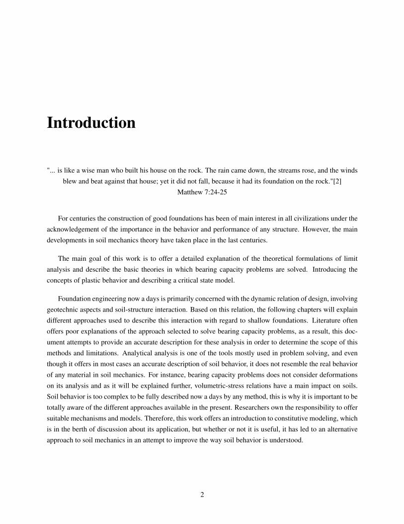
"... is like a wise man who built his house on the rock. The rain came down, the streams rose, and the winds

blew and beat against that house; yet it did not fall, because it had its foundation on the rock."[2]

Matthew 7:24-25

For centuries the construction of good foundations has been of main interest in all civilizations under the

acknowledgement of the importance in the behavior and performance of any structure. However, the main

developments in soil mechanics theory have taken place in the last centuries.

The main goal of this work is to offer a detailed explanation of the theoretical formulations of limit

analysis and describe the basic theories in which bearing capacity problems are solved. Introducing the

concepts of plastic behavior and describing a critical state model.

Foundation engineering now a days is primarily concerned with the dynamic relation of design, involving

geotechnic aspects and soil-structure interaction. Based on this relation, the following chapters will explain

different approaches used to describe this interaction with regard to shallow foundations. Literature often

offers poor explanations of the approach selected to solve bearing capacity problems, as a result, this doc-

ument attempts to provide an accurate description for these analysis in order to determine the scope of this

methods and limitations. Analytical analysis is one of the tools mostly used in problem solving, and even

though it offers in most cases an accurate description of soil behavior, it does not resemble the real behavior

of any material in soil mechanics. For instance, bearing capacity problems does not consider deformations

on its analysis and as it will be explained further, volumetric-stress relations have a main impact on soils.

Soil behavior is too complex to be fully described now a days by any method, this is why it is important to be

totally aware of the different approaches available in the present. Researchers own the responsibility to offer

suitable mechanisms and models. Therefore, this work offers an introduction to constitutive modeling, which

is in the berth of discussion about its application, but whether or not it is useful, it has led to an alternative

approach to soil mechanics in an attempt to improve the way soil behavior is understood.

2

Chapter 1

Bearing Capacity

1.1 Introduction

Soil must be characterized, understood and analyzed previous to any kind of disturbance made over it.

It must be capable as well of carrying the amount of loads placed by any engineered structure, without

displaying excessive settlements or shear failure. For this purpose it is important to have full knowledge

of the ultimate or critical load the soil can bear. Shear failure can induce structure distortion which could

lead to its collapse, while excessive settlements can provoke structural frame damage of the building. The

Ultimate Bearing Capacity (q0) can be understood as the ultimate or maximum load per unit of area the soil

can support before failure. It is also common to address the total bearing capacity in dimensions of force per

unit of length for long, continuous footings. For this scenario it will be given by the symbol Q′0 = q0b. It

has been observed that during a loading process taken to failure, the behavior of the soil displays three and

possibly four stages before failure [20].

1. First Stage: The soil presents distortion, which results in lateral swelling or bulging of the column

of soil beneath the loading area (foundation) and settlement in the surface just beside the foundation

surroundings.

2. Second Stage: The soil around the foundation presents local cracking or shearing.

3. Third Stage: A cone of soil is formed beneath the foundation which induces an outward or downward

movement of the soil.

4. Fourth Stage: In most soils, the shear zone develops sufficiently resulting in a curved surface of

rupture.

3

Bearing Capacity ICIV 200522909

bq0

Figure 1.1: Plastic Analysis

It does not exist any exact mathematical approach for the analysis of such a failure when the ultimate bearing

capacity is exceeded. Therefore, it is necessary to approach the problem under simplifying approximations.

These approximations will be explained in detail in the following document. Even though some of the asser-

tions made in the modeling of foundation problems are incompatible with the observed failure mechanisms

in reality, bearing capacity comparisons made between full sized foundations and mathematical analysis

used, seemed to be quiet similar. These analysis are made regarding soil properties, movement behavior and

the following two assertions.

The Total Bearing Capacity (Q′0) is equal to the resistance offered by the soil beneath the foundation The

soil behavior is analyzed as an ideal plastic material.

Assuming the soil behaves as an ideal plastic material, the solution of problems will be approached under

the limit analysis theorems (Upper and Lower Bound Theorems).

1.2 Bearing Capacity Analysis

The soil beneath the foundation forms a wedge shaped in a cone form which causes a downward punch. This

movement of the wedge induces a lateral movement, resulting in twin zones of shear. Each of these zones

can be described as the composition of a radial and a linear shear acting along the failure surface. Referring

to figure 1.2, the failure mechanism under the foundation can be understood under the interaction of three

major zones. These zones are:

1. Zone BBA, is usually known as the triangular elastic zone, it is located immediately under the bottom

of the foundation. Usually the inclination of the slip planes AB as proposed by Terzagui is α = φ .

2. Zone BCA, is the radial zone of the failure mechanism. It is known as the Prandtl’s radial shear zone.

4


3. Zone BCD, is commonly addressed as the Rankine passive zone. The slip planes BC have an inclina-

tion of 45◦− φ

2 .

Pp φφPp

c cc

cc

cc

c 45°-φ/2A

B

C

Foundation Depth(Df)

bq0

D D

C

B45°-φ/2

α

Figure 1.2: Bearing Capacity Analysis (Shear Zones)

The downward movement of the soil wedge caused by a load Q′0 is resisted by the forces acting on the twin

planes AB. These forces are the resultant of the Pp which acts as a passive pressure, and the cohesion which

acts along the surface AB. The total resistance offered by the wedge in response to the load applied can be

expressed as:

Applying Equilibrium

Q′0 = 2Ppcos(α−φ)+2(ABς sinα) (1.2.1)

By Geometry:

AB =b/2

cosα

Substituting:

Q′0 = 2Pp cos(α−φ)+bς tanα (1.2.2)

The resultant of passive earth pressure Pp can be understood segregating it in three components: Ppγas a

result of the weight of the shear zone ABEC, Ppc produced by the soil cohesion along the rest of the failure

surface, and Ppq produced by the surcharge. The surcharged is defined as as σ0 = γD f (valid only for

homogeneous soils).

All of these components of passive pressure are computed separately, resulting in the following formula.

Q′0 = 2(Ppγ+Ppc +Ppq)cos(α−φ)+bc tanα (1.2.3)

5


Recalling:

Q′0 = q0b

q0 =Q′0b

q0 =2Ppγ

bcos(α−φ)+

[2Ppc cos(α−φ)

b+ c tanα

]+

2Ppq

bcos(α−φ) (1.2.4)

Each of these components of the bearing capacity are in function of the angle of internal friction and the

geometry of the failure zone. This is why the expression for bearing capacity is usually simplified into the

expression (1.2.5):

q0 =γ ′b2

Nγ + c′Nc +σ0Nq (1.2.5)

1.3 Limit Analysis

1.3.1 Introduction

It is of main interest in the analysis of bearing capacity the ultimate load the soil can bear as well as the be-

havior of it during collapse. The analysis of strains during the elastic-plastic range must fulfill the following

criteria:

1. Equilibrium of stresses.

2. Compatibility of strains.

3. σ vs. ε relationship (Hooke’s Law).

If the previous criteria is satisfied simultaneously, any boundary condition could be solved; however, this is

not a handy analysis, determining each condition and behavior of the soil during the whole elastic-plastic

range could be excessively time consuming. To simplify these calculations, the upper and lower bound

theorems are used in order to analyze the behavior of soil during collapse in a more efficient and easy way.

The upper and lower bound theorems are based on the assumption that the soil has a rigid perfectly plas-

tic behavior associated with a flow rule.

Upper Bound Theorem: Kinematically approach. Work done by external forces equated to the rate of dissi-

pation of energy in any chosen mechanism of deformation results in an estimate of the plastic collapse load

that may be equal or higher than the true collapse load. Calladine (1985) refers to this theorem as a geometric

approach to the solution of the problem.

6


Lower Bound Theorem: Is an equilibrium approach. If the external forces applied are in equilibrium with

the internal stress distribution, then load applied on the soil must be safely carried by the foundation. It

represents a safe estimate of the soil strength.

Prior to the modeling of any solution, a kinematically admissible collapse mechanism (Upper Bound) or

a statically admissible stress field (Lower Bound) must be chosen. Satisfying respectively the yield criteria

with regard to the conditions of the problem.

It is important to have in mind that the yield criteria depends on the drainage conditions of the soil. In

the next section both bound theorems will be considered for each drainage condition.

1.3.2 Upper Bound Theorem: Undrained Analysis

1. SLIP CIRCLE MECHANISM This mechanism of failure assumes that failure of the mass of soil

under the foundation happens as a result of the rotation of it with respect to the point 0.

bq0

σ0 σ0

Bdθ

Cu Cu

Cu

Cu

Cu

Cu

Figure 1.3: Slip Circle Mechanism

Work done by external forces.

δE =12

Bdθ(q0−σ0)B (1.3.1)

Energy Dissipated.

δW = πBCuBdθ (1.3.2)

Equating equations 1.3.1 and 1.3.2:

q0 = σ0 +2πCu (1.3.3)

7


2. SLIP CIRCLE MECHANISM (ROTATION CENTER ABOVE FOUNDATION)

This model resembles the failure mechanism analyzed before in most aspects, its only distinction is

that the center of rotation is located above the surface level corresponding with the spot of minimum

safety.

bq0

σ0 σ0

Cu Cu

Cu

Cu

Cu

Rα

O

Figure 1.4: Slip Circle Mechanism Above Surface Level

The width of the foundation by geometry corresponds to:

B = Rsinα (1.3.4)


δE =12

Bdθ(q0−σ0)B (1.3.5)

Energy Dissipated.

δW = πBCuBdθ (1.3.6)

Replacing Equation 1.3.4 in 1.3.5 and 1.3.6:

δE =12

Rsinαdθ(q0−σ0)Rsinα (1.3.7)

δW = 2αRCuRdθdθ (1.3.8)


(q0−σ0) =4α

sin2α

Cu (1.3.9)

8


Derivating the previous expression with respect to α and equating the result to Zero it is possible to

optimize the value of the angle and determine q0.

q0

∂α= 4Cu

(sin2

α−2α sinα cosα

sin4α

)=

4Cusin2 α

(1− 2α

tanα

)=

4Cusin2

α

(1− 2α

tanα

)= 0

⇒ tanα = 2α

Solving:

α = 67◦ or 1.17rad

Replacing the previous value in the equation 1.3.9, the expression can be simplified into q0 and σ0

terms.

(q0−σ0) =4α

sin2α

Cu (1.3.10)

q0 = σ0 +5.52Cu (1.3.11)

EXAMPLE 1: Minimum Safety

The following example shows the relation between the height chosen and the maximum bear capacity

for the solution of a slip circle collapse mechanism when the center of rotation is above the surface

level. The height chosen corresponds to the minimum bear capacity labeled in the graph 1.5.

Problem Conditionsσ0 (kPa) cu (kPa) b (m)

45 12 4

Table 1.1: Example1 (Problem Conditions)

9


q0 (kPa) r (m) h (m) α (rad) α (Degrees)120,40 4,00 0,00 0,00 0,00113,05 4,10 0,90 1,35 77,32111,73 4,20 1,28 1,26 72,25111,29 4,30 1,58 1,20 68,47111,25 4,33 1,66 1,18 67,49111,24 4,35 1,70 1,17 67,00111,27 4,40 1,83 1,14 55,38111,52 4,50 2,06 1,09 62,73114,55 5,00 3,00 0,93 53,13120,82 5,70 4,06 0,78 44,57127,96 6,40 5,00 0,68 38,68136,61 7,20 5,99 0,59 33,75

Table 1.2: Minimum Safety Calculation

4 5 6 7 8Radius r [m]

110

120

130

140

Bea

ring

Cap

acity

q [k

Pa]

120.4

113.1

111.2

114.5

120.8

128

136.6

Figure 1.5: Minimum Safety Plot

3. SLIDING RIGID BLOCKS The following collapse mechanism is analyzed under the assumption

of an articulated structure made of rigid blocks. The rigid block under the foundation is supposed to

move downward under the influence of a velocity V, causing a lateral movement of the middle one

resulting in an upward push of the last block. Movements are resisted by friction on each slip plane by

different velocities.

10


bq0

σ0 σ0

V

V2

V3

V2

V3V1 V1

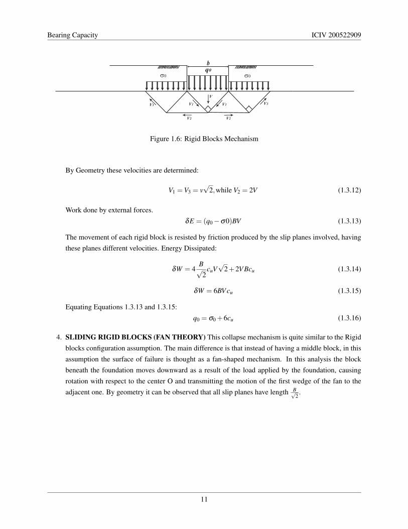
Figure 1.6: Rigid Blocks Mechanism

By Geometry these velocities are determined:

V1 = V3 = v√

2,while V2 = 2V (1.3.12)


δE = (q0−σ0)BV (1.3.13)

The movement of each rigid block is resisted by friction produced by the slip planes involved, having

these planes different velocities. Energy Dissipated:

δW = 4B√2

cuV√

2+2V Bcu (1.3.14)

δW = 6BV cu (1.3.15)

Equating Equations 1.3.13 and 1.3.15:

q0 = σ0 +6cu (1.3.16)

4. SLIDING RIGID BLOCKS (FAN THEORY) This collapse mechanism is quite similar to the Rigid

blocks configuration assumption. The main difference is that instead of having a middle block, in this

assumption the surface of failure is thought as a fan-shaped mechanism. In this analysis the block

beneath the foundation moves downward as a result of the load applied by the foundation, causing

rotation with respect to the center O and transmitting the motion of the first wedge of the fan to the

adjacent one. By geometry it can be observed that all slip planes have length B√2.

11


bq0

σ0 σ0

VCu

Cu

Cu Cu

Cu

Cu

Figure 1.7: Collapse Mechanism (Shear Fan)


δE = (q0−σ0)BV (1.3.17)

Energy Dissipated. For this calculation it is necessary to analyze each surface, including the energy

dissipated by the shear fan. For the slip planes:

δW1 = 2B√2

cuV√

2+b√2

π

2cuV√

2 (1.3.18)

δW1 = V Bcu(2+π

2) (1.3.19)

Energy dissipated by the fan.

δW2 =∫

π/20cu

b√2

v√

2dθ = cuBVπ

2(1.3.20)

The total energy dissipated can be estimated by adding 1.3.19 and 1.3.20:

δW = cuBV (2+π) (1.3.21)


q0 = σ0 +5.14cu (1.3.22)

LOWEST UPPER BOUND SOLUTION commonly known as Prandtl solution.[1]

1.3.3 Lower Bound Theorem: Undrained Analysis

1. Stress Field (Single Discontinuity) A vertical discontinuity located under one edge of the foundation

is considered for this analysis. The stress field for this conditions will be understood under the absence

of shear stresses, this means, vertical and horizontal stresses will be major.

12


At point A the magnitude of the vertical stress is σA = σ0 which rotates and angle π

2 to reach point B

at the the discontinuity.

bq0

σ0 σ0

A

B

C

Figure 1.8: Stress Field (One Discontinuity)

Drawing the Mohr’s circles it is possible to determine σB and σC, recalling this is an undrained behav-

ior problem the radius of each circle will be equal to cu.

BA C σ

τ

σ0 2cu 2cu

Figure 1.9: Mohr’s Circles (Undrained Behavior)

Under this analysis it is possible to determine the maximum lower bound value.

σC = 4cu +σ0⇒ q0 = σ0 +4cu (1.3.23)

Assuming the correct solution for this kind of problem was correctly approached and determined in

the upper bound analysis as q0 = σ0 +5.14cu, the previous value for the lower bound failure loading q0

is considerably distanced from being correct. As much as it is a safe approximation, the main concern

of this work is to determine a more exact value wherever is possible.

13


2. Stress Field (Various Discontinuities) Using various discontinuities above the foundation it is pos-

sible to obtain a better solution. It must be clear that each discontinuity added to the problem simply

adds one more change in the direction of the major principal stress. For symmetry purposes in the

following analysis the changes in direction across each discontinuity will be assumed equal. In the

previous solution the direction of the major principal stress changes by 90 degrees across one discon-

tinuity, this means, the changes in direction across a number n of discontinuities must total the same

90 degrees.

Once each circle is determined the value of the ultimate lower bound can be easily calculated. The

following analysis is done with a stress field containing a stress fan and shows how Mohr’s circles are

depicted. The procedure for plotting the Mohr’s circles is as follows (Using pole points).

• Each circle represents one of the zones in which the the soil beneath the foundation was divided

by the arrange of discontinuities. The first circle must be drawn with center Center1 = σ0 + cu

and Radius cu.

• It is important to recall that two pole points can be established in the same circle. For this

analysis the pole point considered will be the one relating to the direction of the planes on which

the stresses are acting. Therefore, the pole point p1 for the first circle will be found by projecting

an horizontal line from σ0 to intersect circle 1.

• After the rotation angle across each discontinuity is determined, any stress point S common to

two zones is easily determined by projecting a line from the pole of the circle. This line must be

parallel to the discontinuity plane, regarding the zone that is being analyzed.

• The center of the stress circle adjacent to the previous zone plotted, is found by completing the

equilateral triangle formed by the stress point S and the center of the circle already drawn. This

new circle must have radius cu and must pass through point S.

• Regardless of the number of discontinuities chosen for the analysis, each step mentioned before

must be followed for plotting the remaining circles until the last zone is reached.

• The major principal stress of the last circle is equal to the lowest bound failure solution for the

problem.

EXAMPLE 2: Stress Field (Two Discontinuities)

The following example is done for the analysis of a shallow foundation under the assumption of two

discontinuities located beneath it. The angle chosen is 45 degrees separating both discontinuities from

each other.

14


bq0

σ0 σ0

A

45

D

C B

Figure 1.10: Stress Field (Two Discontinuities)

The Mohr’s circles were drawn using the pole points procedure, which are labeled as P(n) for each

circle.

B

A

C

D σ

τ

σ0 cu cu cu

P145

P2

P3

Figure 1.11: Mohr’s Circles (Two Discontinuities)

For this analysis the result for the ultimate bearing capacity is:

q0 = σ0 +2cu +2√

2cu⇒ q0 = σ0 +4.83cu (1.3.24)

3. Stress Field (Stress Fan) This stress field is composed by a stress fan located beneath the foundation.

For the analysis of this large amount of discontinuities the following analysis is done. The Mohr’s

circles plotted below were drawn under the consideration that the first discontinuity is rotated 45

degrees. Therefore, in the Mohr analysis the angle has a rotation of 90 degrees and σB = σ0 + cu.

Recall σA = σ0. This analysis must be made for the total amount of discontinuities in order to be able

to determine the total stress at D and determine the ultimate lower bound value.

15


bq0

σ0 σ0

A

B

D

C

Figure 1.12: Stress Field (Stress Fan)

First of all it is important to define the mean stress acting on each body analyzed. The mean stress will

be understood as the difference of the normal stresses components acting between two discontinuities.

It will be denoted as ∆p.

B

A

C

D σ

τ

π/2

dθ

σ0 cu πcu cu

Figure 1.13: Stress Field (Stress Fan)

∆p = p2− p1 = 2cu sindθ ≈ 2cudθ

For this analysis:

d p =∫

π/2

02cudθ = πc2

This means the total ∆p along the stress fan will be equal to πc2. With this value, the stress at point D

can be easily determined and equated to q0.

q0 = σ0 +πcu +2cu

q0 = σ0 +5.14cu

(1.3.25)

This result is equal to the ultimate upper bound value calculated in the kinematic analysis using the

rigid block (shear fan) collapse mechanism. Therefore, this is an EXACT PLASTIC SOLUTION for

the maximum bearing capacity.[14]

16


1.3.4 Upper Bound Theorem: Drained Analysis

1. Logarithmic Spiral Shaped Collapse Mechanism This analysis is made under the assumption that

plastic deformations occur fulfilling the criterion of normality (Associated flow rule). The soil is

supposed weightless. Since the internal work done on a normal stress cancels out the work done on the

corresponding shear stress, it is possible to find this kinematically admissible solution by calculating

the work done by the the external loads and equating it to zero. The failure surface of the following

collapse mechanism resembles the equation:

R2

R1= exp(θ tanϕ

′) (1.3.26)

where ϕ ′ is the effective angle of shearing resistance of the soil, and θ the angle made by R1 and R2.

According to picture 1.14 and the previous formula, the distance BD = b[exp(π tanϕ ′)], where R1 =b, R2 = BD, and θ = π .

bq0

R1 R2

B Dbdθ dθ

σ0σ0

Figure 1.14: Spiral Shaped Collapse Mechanism

The external load q0 forces the soil beneath the foundation for this collapse mechanism to rotate by an

angle dθ from the bottom of the foundation. This rotation causes the surface BD to rotate by the same

angle, causing an upward displacement.

By geometry it is possible to determine the total work done by the external loads. Analyzing the

upward displacement of the surface BD the work done by that movement is calculated. For this matter

work will be defined as the change of energy needed to perform an action. Calculating the area of soil

pushed upward next to the foundation and approximating it to the shape of a triangle, the problem is

nearly solved . For this problem the work done by σ0 is the potential of energy available to prevent the

upward displacement and is equal to Area∗σ0.

17


dθ

D

B

dθ

Figure 1.15: Rotation Approximation (Not in Scale)

Therefore the total work done is:

δE = q0b2

2dθ −σ0

b2

2dθ [exp(2π tanϕ

′)] (1.3.27)

Equating it to zero, and solving for q0, the ultimate bearing capacity is:

q0 = σ0exp(2π tanϕ′) (1.3.28)

EXAMPLE 3: Logarithmic Spiral Shaped Collapse Mechanism

The following collapse mechanism describes the failure surface of the logarithmic equation presented

in the previous analysis. For this analysis the width chosen for the footing was 4 meters and the the

corresponding angle of shearing resistance for the soil ϕ ′ = 20◦.

16 12 8 4 0 -4 -8 -12X [m]

16

12

8

4

0

Y [m

]

0

1.883

3.982

5.8997.14 7.196

5.653

2.314

0

1.883

3.982

5.8997.147.196

5.653

2.314

Figure 1.16: Example 3: Logarithmic analysis

2. Rigid Blocks (Shear Fan) This mechanism is depicted by two rigid blocks joined by a shear fan

shaped failure surface. The angle formed by the surface of both rigid blocks is 90◦. The shear fan

surface is described by the same logarithmic function of the previous collapse mechanism analyzed.

18


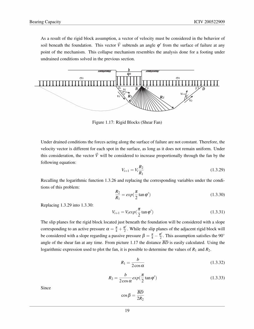
As a result of the rigid block assumption, a vector of velocity must be considered in the behavior of

soil beneath the foundation. This vector ~V subtends an angle ϕ ′ from the surface of failure at any

point of the mechanism. This collapse mechanism resembles the analysis done for a footing under

undrained conditions solved in the previous section.

bq0

R1 R2

B D

σ0σ0

V2

V1

Vi

Vi+1 ϕ’ ϕ’

α β β

Figure 1.17: Rigid Blocks (Shear Fan)

Under drained conditions the forces acting along the surface of failure are not constant. Therefore, the

velocity vector is different for each spot in the surface, as long as it does not remain uniform. Under

this consideration, the vector ~V will be considered to increase proportionally through the fan by the

following equation:

Vi+1 = ViR2

R1(1.3.29)

Recalling the logarithmic function 1.3.26 and replacing the corresponding variables under the condi-

tions of this problem:R2

R1= exp(

π

2tanϕ

′) (1.3.30)

Replacing 1.3.29 into 1.3.30:

Vi+1 = Viexp(π

2tanϕ

′) (1.3.31)

The slip planes for the rigid block located just beneath the foundation will be considered with a slope

corresponding to an active pressure α = π

4 + ϕ ′

2 . While the slip planes of the adjacent rigid block will

be considered with a slope regarding a passive pressure β = π

4 −ϕ ′

2 . This assumption satisfies the 90◦

angle of the shear fan at any time. From picture 1.17 the distance BD is easily calculated. Using the

logarithmic expression used to plot the fan, it is possible to determine the values of R1 and R2.

R1 =b

2cosα(1.3.32)

R2 =b

2cosαexp(

π

2tanϕ

′) (1.3.33)

Since

cosβ =BD2R2

19


⇒ BD =bcosβ

cosαexp(

π

2tanϕ

′) (1.3.34)

Simplifying the previous expression it is possible to observe that for this scenario cosβ

cosα= tanα .

cosβ

cosα=

cos(π/4)cos(ϕ ′/2)+ sin(π/4)sin(ϕ ′/2)cos(π/4)cos(ϕ ′/2)− sin(π/4)sin(ϕ ′/2)

=cos(ϕ ′/2)+ sin(ϕ ′/2)cos(ϕ ′/2)− sin(ϕ ′/2)

In the other hand:

tanα =tan(π/4)+ tan(ϕ ′/2)

1− tan(π/4) tan(ϕ ′/2)

=1+ sin(ϕ ′/2)

cos(ϕ ′/2)

1− sin(ϕ ′/2)cos(ϕ ′/2)

=cos(ϕ ′/2)+ sin(ϕ ′/2)cos(ϕ ′/2)− sin(ϕ ′/2)

Finally the distance BD given by equation 1.3.34 can be simplified to the following expression:

BD = b tanαexp(π

2tanϕ

′) (1.3.35)

Prior to solving this problem it is important to recall that soil has been assumed weightless and co-

hesionless. Since only the vertical components of velocity are of interest for computing the area, the

vertical displacement of each rigid block must be determined.

Vy1 = Vi sin(α−ϕ′) = Vi sinβ (1.3.36)

Vy2 = Vi+1 sin(β +ϕ′) = Vi+1 sinα (1.3.37)

Replacing Vi+1 using equation 1.3.31:

Vy2 = Viexp(π

2tanϕ

′)sinα (1.3.38)

Now the total change of energy can be evaluated:

δE = q0bVy1−σ0BDVy2 (1.3.39)

Replacing 1.3.36 and 1.3.38 into 1.3.39:

δE = q0bVi sinβσ0b tanαexp(π

2tanϕ

′)Viexp(π

2tanϕ

′)sinα (1.3.40)

20


Equating to Zero:

q0 sinβ = σ0sin2

α

cosαexp(π tanϕ

′) (1.3.41)

Since sinβ = cosα

q0 = σ0exp(π tanϕ′) tan2

α

The lowest obtainable upper bound solution is (Replacing α):

q0 = σ0exp(π tanϕ′) tan2

(π

4+

ϕ ′

2

)(1.3.42)

LOWEST UPPER BOUND SOLUTION[1]

1.3.5 Lower Bound Theorem: Drained Analysis

Prior to the solving of any collapse mechanism a statically admissible stress field must be satisfied. The

effective stress failure criterion must be fulfilled too. For this analysis full dissipation of excess pore pressure

is assumed and soil is supposed to be cohesionless. As well as it was done in section 1.3.3, a different number

of stress discontinuities will be used to approach the maximum obtainable lower bound solution.

1. Stress Field (Single Discontinuity) For this problem a single discontinuity located right beneath one

edge of the foundation is assumed. Since the angle of shearing resistance of the soil is known and the

soil is supposed cohesionless, it is possible to draw the Mohr’s circles corresponding to the stress field

conditions depicted in the following picture.

bq0

σ0 σ0

A

B

C

σC σA

σB

Figure 1.18: Stress Field (One Discontinuity)

At point A the magnitude of the vertical stress is σA = σ0 which rotates an angle π

2 to reach point B

at the the discontinuity; therefore, the horizontal stress at that point is considered major. The failure

criterion is satisfied since each one of the circles touches the failure envelope.

21


BA σ

τ

σ0

C

ϕ’

σ1 σ2O

M

N

R1

R2

Figure 1.19: Mohr’s Circles for a Single Discontinuity

From geometry it is possible to calculate the value for σC which will be equal to the ultimate bearing

capacity for this problem.

σC = σ2 +R2 (1.3.43)

Where σ2 is the center, and R2 is the radius corresponding to the circle representing the zone located

under the foundation.

R2 = σ2 sinϕ′

R2 = σ2−σB

(1.3.44)

Equating equations 1.3.43 and 1.3.44.

σB = σ2−σ2 sinϕ′ (1.3.45)

σ2 =σB

1− sinϕ ′

R2 = σB

(sinϕ ′

1− sinϕ ′

) (1.3.46)

Replacing equations 1.3.46 into 1.3.43:

σC = σB

(1+ sinϕ ′

1− sinϕ ′

)(1.3.47)

Following the same procedure is possible to determine the value for 1.3.45 using equations 1.3.46. For

this scenario:

σB = σ0

(1+ sinϕ ′

1− sinϕ ′

)(1.3.48)

22



σC = σ0

(1+ sinϕ ′

1− sinϕ ′

)2

(1.3.49)

2. Stress Field (Two Discontinuities) As seen from the lower bound analysis done for Undrained prob-

lems, the use of various discontinuities represents the best approach to the solution of the problem.

bq0

σ0 σ0

A

B

D

σD σA

σBC σC

Figure 1.20: Stress Field (Two Discontinuities)

From geometry it is possible to seek for a general solution for this kind of problem. The normal and

shear stress corresponding to each discontinuity are labeled in the Mohr’s circles shown in picture 1.21.

The angle δ ′ represents the angle made with the horizontal of the line made through the intersections

of the drawn circles. For this scenario this line passes through the origin O, B, and C. Lets denote this

line as the "intersect line". It is also useful to introduce an angle ∆, angle drawn between the intersect

line at the discontinuity point and the radius of each circle.

23


A σ

τ

σ0

ϕ’

P1

P2

P3

B

C

D

δ’

Δ−δ’

Δ−δ’

Δ+δ’

O

ΔΔ

Δ

Δ

σ1 σ2 σ3

Figure 1.21: Mohr’s Circles for Two Discontinuities

Some triangles have been isolated in order to understand more clearly the procedure followed.

B

Δδ’

OR1

σ1

Figure 1.22: Isolated Triangle 1

C

σ2O

Δ

δ’ 180−Δ−δ’

R2


24


O

R1

σ1ϕ


C

Δ−δ’O

δ’

180−Δ R3

σ3


From figure 1.23:sinδ ′

R2=

sin∆

σ2(1.3.50)

From figure 1.24:

σ2 =R2

sinϕ ′(1.3.51)


sin∆ =sinδ ′

sinϕ ′(1.3.52)

Since δ ′ and ϕ ′ are known is possible to determine ∆. The change in stress state from σ2 to σ3 is

solved from figure 1.23 and 1.25.

sin(180−∆−δ )OC

=sin(∆)

σ2

sin(∆−δ )OC

=sin(180−∆)

σ3

Since sin(180−∆) = sin∆ and sin(180−∆− δ ) = sin(∆ + δ ). Eliminating OC from the previous

equations.σ3

σ2=

sin(∆+δ )sin(∆−δ )

(1.3.53)

25


Since the stress conditions for σD can be easily determined referring to figure 1.21, it is possible to

establish a general solution for this scenario (weightless, cohesionless).

σD = σ3(1+ sinϕ′) (1.3.54)

σ2′ = σ2(1− sinϕ′) (1.3.55)

Replacing 1.3.53 and 1.3.55 into 1.3.54:

σD = σ2′sin(∆+δ )sin(∆−δ )

(1+ sinϕ ′)(1− sinϕ ′)

(1.3.56)

For this problem:

σ2′ = σAsin(∆+δ )sin(∆−δ )

(1.3.57)

Substituting 1.3.57 in 1.3.56, the lower bound solution for this scenario is:

σD = σA

(sin(∆+δ )sin(∆−δ )

)2 (1+ sinϕ ′)(1− sinϕ ′)

(1.3.58)

The procedure followed above can be performed for any number of discontinuities n.

Expression 1.3.58 can be generalized into:

σD = σA

(sin(∆+δ )sin(∆−δ )

)n (1+ sinϕ ′)(1− sinϕ ′)

(1.3.59)

Equation which can be written in terms of a dimensionless factor Nq

σD = σANq (1.3.60)

Since σA = σ0.

⇒ σD = σ0Nq (1.3.61)

Where Nq[14]:

Nq =(


)n (1+ sinϕ ′)(1− sinϕ ′)

(1.3.62)

26


1.3.6 Weight and Cohesion Influence on Soils

1. Weight InfluencePrevious analysis were made under the assumption that soil is weightless and cohesionless for drained

scenarios, approximations which may lead to underestimated values for the ultimate bearing capacity

of the soil q0. Literature offers different approaches for weight effects on bearing capacity calculations,

authors such as Sokolovski, Prandtl or Coulomb have suggested various mechanisms in which the

weight influence can be related into bearing capacity equations. Using the Coulomb mechanism it is

possible to determine the soil weight contribution to the ultimate bearing capacity.

Foundations are usually constructed at some depth D f beneath the surface, as labeled in figure 1.2,

this depth of soil is considered only as a surcharge and it does not contribute to the shear strength.

When D f 6 b the soil weight makes a considerable contribution to the ultimate bearing capacity. The

following approximation is done using the Coulomb failure mechanism 1.26. The vertical line plot

joining the points B and C divides the active and passive zone beneath the foundation. Since the

stresses across the discontinuity can not be equated, the procedure followed is to equate the active and

passive forces acting along the discontinuity.

bq0γ

B D

ϕΑ

σ0σ0

ϕP

Y = b*tan(ϕΑ)C

Figure 1.26: Coulomb Failure Mechanism

Recalling from soil mechanics theory, it is possible to relate the vertical and horizontal stress acting

on the same body. This relation is given by the earth pressure coefficient denoted as K. The active

and passive vertical stress distributions are drawn in figure 1.27. Calculating the area of the stress

distributions it is possible to estimate the active and passive forces acting along the discontinuity BC

over a specified depth Y .σH

σV= K (1.3.63)

The active and passive earth pressure coefficients of lateral stress are given by KA and KP respectively.

The active pressure zone is the zone located just beneath the foundation, the angle of the slip plane

is ϕA = 45◦+ ϕ ′/2. In the other hand, the zone located outside the loaded area will be considered

passive, as this zone restrains the movement of the active wedge.

27


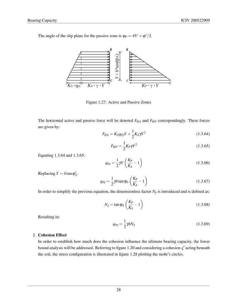
The angle of the slip plane for the passive zone is ϕP = 45◦+ϕ ′/2.

KA * q0γ KA * γ * Y

B

CKP * γ * Y

B

C

Y =

b*ta

n(ϕΑ

)

Figure 1.27: Active and Passive Zones

The horizontal active and passive force will be denoted FHA and FHP correspondingly. These forces

are given by:

FHA = KAq0γY +12

KAγY 2 (1.3.64)

FHP =12

KPγY 2 (1.3.65)

Equating 1.3.64 and 1.3.65:

q0γ =12

γY(

KP

KA−1)

(1.3.66)

Replacing Y = b tanϕ ′A.

q0γ =12

γb tanϕA

(KP

KA−1)

(1.3.67)

In order to simplify the previous equation, the dimensionless factor Nγ is introduced and is defined as:

Nγ = tanϕA

(KP

KA−1)

(1.3.68)

Resulting in:

q0γ =12

γbNγ (1.3.69)

2. Cohesion EffectIn order to establish how much does the cohesion influence the ultimate bearing capacity, the lower

bound analysis will be addressed. Referring to figure 1.20 and considering a cohesion ς ′ acting beneath

the soil, the stress configuration is illustrated in figure 1.28 plotting the mohr’s circles.

28


A σ

τ

ϕ’

P1

P2

P3

B

C

D

δ’

Δ−δ’

Δ−δ’

Δ+δ’

O

ΔΔ

Δ

Δ

σ1 σ2 σ3

cΔσ

Figure 1.28: Mohr’s Circles for Two Discontinuities (Cohesion Soil)

It is easily observed that the effect of cohesion is to increase all normal stresses by an amount equal to

∆σ for any scenario. By geometry:

∆σ = c′ cotϕ′ (1.3.70)

Therefore:

σA = σ0 +∆σ (1.3.71)

q0 = σD +∆σ (1.3.72)

σA = σ0 + c′ cotϕ′ (1.3.73)

σD = q0 + c′ cotϕ′ (1.3.74)

1.4 Formulating Bearing Capacity Equations

Limit Analysis has been the tool used to theoretically approach the ultimate bearing capacity q0 of the soil

beneath a shallow foundation. In order to formulate a single expression relating the conditions (Drained -

Undrained), and parameters of the soil it is necessary to compute some of the results deduced in the previous

sections.

29


Computing into a single equation the soil weight and shear strength of the soil, it is possible to formulate

a single equation to calculate the ultimate bearing capacity in terms of the shear strength angle φ . Since the

net effect do to the soil weight is proportional to the foundation depth of it’s failure zone. The soil effect can

be added into equation 1.3.42. Considering the pressure due to the extra soil weight, the net effect will be

reflected by the increase of all normal stresses by an amount σ ′ = γ ′b tanφ ′A as is illustrated in figures 1.26

and 1.27. Therefore, for a normal load applied over a continuous foundation, equation 1.3.42 is altered into:

q0 + γ′b tanφ

′A =

(σ0 + γ

′b tanφ′)exp(π tanϕ

′) tan2(

π

4+

ϕ ′

2

)(1.4.1)

Simplifying the previous expression by introducing the dimensionless factor Nq and analyzing the failure

mechanism under the Terzagui assumption of ϕ ′A = ϕ ′ :

Nq = tan2(

π

4+

ϕ ′

2

)(1.4.2)

Equation 1.4.1 can be rearranged into:

q0 = σ0Nq + γ′b tanφ

′(Nq−1) (1.4.3)

Finally computing equations 1.3.73 and 1.3.74 into 1.4.3 is possible to include the cohesion effect due to the

shear strength of the soil.

q0 + c′ cotϕ′ = (σ0 + c′ cotϕ

′)Nq + γ′b tanφ

′(Nq−1) (1.4.4)

Rearranging equation 1.4.4:

q0 = σ0Nq + c′ cotϕ′(Nq−1)+ γ

′b tanφ′(Nq−1) (1.4.5)

Equation 1.4.5 can be expressed in terms of Nγ ,NC and Nq and can be rewritten as equation 1.2.5 formulated

in section 1.2:

q0 =γ ′b2

Nγ + c′Nc +σ0Nq

Where:

Nq = exp(π tanϕ′) tan2

(π

4+

ϕ ′

2

)(1.4.6)

Nc = cotφ′(Nq−1) (1.4.7)

Nγ = 2tanφ′(Nq−1) (1.4.8)

It is important to recall that for undrained conditions as it was deduced in section 1.3.2 and 1.3.3 Nq = 1,

Nc = (2+π) and Nγ = 0. Therefore, the ultimate bearing capacity for a strip footing, continuous, of infinite

30


length and width b from equation 1.2 is reduced to:

q0 = σ0 + cuNc (1.4.9)

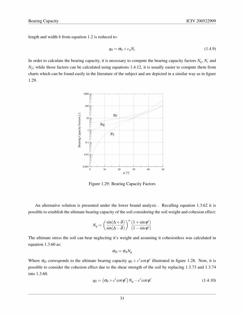
In order to calculate the bearing capacity, it is necessary to compute the bearing capacity factors Nq, Nc and

Nγ ; while those factors can be calculated using equations 1.4.12, it is usually easier to compute them from

charts which can be found easily in the literature of the subject and are depicted in a similar way as in figure

1.29.

0 10 20 30 40 50ϕ' [º]

0.001

0.01

0.1

1

10

100

1000

Bea

ring

Cap

acity

Fac

tors

[-]

Nc

Nq

Nγ

Figure 1.29: Bearing Capacity Factors

An alternative solution is presented under the lower bound analysis . Recalling equation 1.3.62 it is

possible to establish the ultimate bearing capacity of the soil considering the soil weight and cohesion effect:

Nq =(


)n (1+ sinϕ ′)(1− sinϕ ′)

The ultimate stress the soil can bear neglecting it’s weight and assuming it cohesionless was calculated in

equation 1.3.60 as:

σD = σANq

Where σD corresponds to the ultimate bearing capacity q0 + c′ cotϕ ′ illustrated in figure 1.28. Now, it is

possible to consider the cohesion effect due to the shear strength of the soil by replacing 1.3.73 and 1.3.74

into 1.3.60.

q0 =(σ0 + c′ cotϕ

′)Nq− c′ cotϕ′ (1.4.10)

31


Finally the soil effect can be computed adding equation 1.3.69 and 1.4.10

q0 =γ ′b2

Nγ + c′ cotϕ′Nq− c′ cotϕ

′+σ0Nq (1.4.11)

Rearranging it is possible to formulate once again the bearing capacity equation in it’s classical way 1.2.5 :

q0 =γ ′b2

Nγ + c′ϕ ′Nc +σ0Nq

Where:

Nq =(


)n (1+ sinϕ ′)(1− sinϕ ′)

(1.4.12)

Nγ = tanϕA

(KP

KA−1)

(1.4.13)

Nc = cotϕ′(Nq−1) (1.4.14)

Alternative values to calculate the bearing capacity factors can be found depending on the method or analysis

used to approach the problem as it was seen in this chapter. Different authors have made different approaches,

regarding the failure mechanisms, and several assumptions. For instance, Meyerhof differs from Terzagui

in different aspects. First of all, the angle ϕ ′A of the wedge, Meyerhof does not assume it to be equal to

ϕ ′ causing the failure mechanism to extend deeper. Second of all, Meyerhof suggests that the shear zone

extends above the foundation level (figure 1.30).

bq0

B

Dσ0

90 - ϕ

90 - ϕ

Figure 1.30: Meyerhof Failure Mechanism

These assumptions, as well as many others made by different authors have led to several equations with

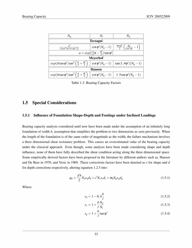
the bearing capacity factors modified. Table 1.3 presents some of the bearing capacity equations suggested

by Terzagui, Meyerhof and Hansen.

32


Nq Nc Nγ

Terzaguia2

2cos2(π/4+ϕ ′/2) cotϕ ′(Nq−1) tanϕ ′

2

(KP

cos2 ϕ ′−1)

a = exp[(43 π− ϕ ′

2 ) tanϕ ′]Meyerhof

exp(π tanϕ ′) tan2(

π

4 + ϕ ′

2

)cotϕ ′(Nq−1) tan(1,4ϕ ′)(Nq−1)

Hansenexp(π tanϕ ′) tan2

(π

4 + ϕ ′

2

)cotϕ ′(Nq−1) 1,5tanϕ ′(Nq−1)

Table 1.3: Bearing Capacity Factors

1.5 Special Considerations

1.5.1 Influence of Foundation Shape-Depth and Footings under Inclined Loadings

Bearing capacity analysis considered until now have been made under the assumption of an infinitely long

foundation of width b, assumption that simplifies the problem to two dimensions as seen previously. When

the length of the foundation is of the same order of magnitude as the width, the failure mechanism involves

a three dimensional shear resistance problem. This causes an overestimated value of the bearing capacity

under the classical approach. Even though, some analysis have been made considering shape and depth

influence, none of them have fully described the shear condition acting along the three dimensional space.

Some empirically derived factors have been proposed in the literature by different authors such as, Hansen

and De Beer in 1970, and Vesic in 1969. These corrections factors have been denoted as s for shape and d

for depth corrections respectively, altering equation 1.2.5 into:

q0 =γ ′b2

Nγsγdγ + c′Ncscdc +σ0Nqsqdq (1.5.1)

Where:

sγ = 1−0,4bl

(1.5.2)

sc = 1+bl

Nq

Nc(1.5.3)

sq = 1+bl

tanϕ′ (1.5.4)

33


dγ = 1 (1.5.5)

dc = 1+0,4ξ (1.5.6)

dq = 1+ξ tanϕ′(1− sinϕ

′) (1.5.7)

And:

ξ =D f

bfor

D f

b6 1 or ξ = tan−1 D f

bif

D f

b> 1

Assuming the load applied over the foundation is inclined at an angle ψ with respect to the vertical axis,

only a fraction of the load will be applied normal to the foundation while the rest will act as an horizontal

component (figure 1.31). Meyerhof and Hanna in 1981, proposed the following correction regarding a

problem under an inclined load.

Iγ =(

1− ψ◦

ϕ ′

)2

(1.5.8)

Ic = Iq =(

1− ψ◦

90

)2

(1.5.9)

Foundation Depth (Df)

b

Q0

ψ

Figure 1.31: Inclined Load

Since the ultimate load q0 is expressed per linear meter, equation 1.5.1 is altered into expression 1.5.10

which considers the effects of an inclined load.

q0 = L(

γ ′b2

Nγsγdγ Iγ + c′NcscdcIc +σ0NqsqdqIq

)(1.5.10)

With L as the foundation length. It is important to recall that equation 1.5.10 is used for drained analysis,

where the velocity of the applying load is less than the velocity of draining water. For undrained analysis,

the ultimate bearing capacity is simplified into expression 1.5.11:

q0 = L(σ0 + cuNcscdcIc) (1.5.11)

34


1.5.2 Load Eccentricity

A footing is eccentrically loaded when the load applied over it does not act over the center of mass of the

footing causing the foundation to be subject to a moment Mx = Q0e or My = Q0e . Where e corresponds

to the eccentric length. Another scenario for eccentric loads happens when, regardless if the load is applied

over the center it is is subject to a moment too. For this scenario it is possible to find the equivalence length e

that produces that moment. Since the gravitational forces (self weight) are uniform in the footing, the center

of gravity corresponds to the center of mass of the foundation. Eccentricity is defined as the length measured

from the point where the load is applied to the center of gravity. Therefore, it can be understood in a single

way or as a two way eccentricity.[1]

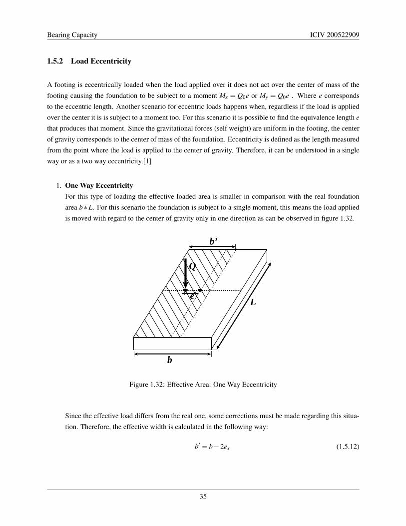
1. One Way EccentricityFor this type of loading the effective loaded area is smaller in comparison with the real foundation

area b∗L. For this scenario the foundation is subject to a single moment, this means the load applied

is moved with regard to the center of gravity only in one direction as can be observed in figure 1.32.

Q

e

b’

b

L

Figure 1.32: Effective Area: One Way Eccentricity

Since the effective load differs from the real one, some corrections must be made regarding this situa-

tion. Therefore, the effective width is calculated in the following way:

b′ = b−2ex (1.5.12)

35


If the eccentricity is aligned in the other axis, the effective length will be:

L′ = b−2ey (1.5.13)

Once the effective width of the foundation b′ is calculated, the ultimate bearing capacity can be com-

puted using the previous formulas addressed in this chapter in conjunction with b′. Since the eccen-

tricity changes the stress distribution beneath the foundation, it can not be longer assumed uniform. A

schematic stress distribution due to the load eccentricity is shown in figure 1.33.

b

Q

e

qmin

qmax

Df

Figure 1.33: Stress Distribution Due to a Load Eccentricity

From the stress distribution is possible to determine the optimum values corresponding to qmin and

qmax.

qmin =Qbl− bM

2I(1.5.14)

qmax =Qbl

+bM2I

(1.5.15)

where M denotes the moment M = Qe and I represents the moment of inertia defined as I = lb3/12.

Replacing M and I into 1.5.14 and 1.5.15.

qmin =Qbl

(1− 6e

b

)(1.5.16)

qmax =Qbl

(1+

6eb

)(1.5.17)

From equation 1.5.16 it is possible to establish that for eccentricity values e bigger than b/6, qmin

becomes negative, implying an upward movement or lifting off the ground on one of the sides. There-

fore, it is necessary to guaranty on the design of any foundation that the stress distribution remains

positive in every single spot beneath it. This is why, in order to prevent bearing capacity failure the

following criterion must be satisfied:

e 6b6

(1.5.18)

36


2. Two Way EccentricityA foundation subject to eccentricity in both directions has an effective area similar to the one hatched

in figure 1.34. For this scenario the effective width of the foundation can be calculated as:

b′ =b−b1

2+

L1(b−b1)2L

(1.5.19)

Q

b1

b

Lex

eyL1

Figure 1.34: Effective Area: Two Way Eccentricity

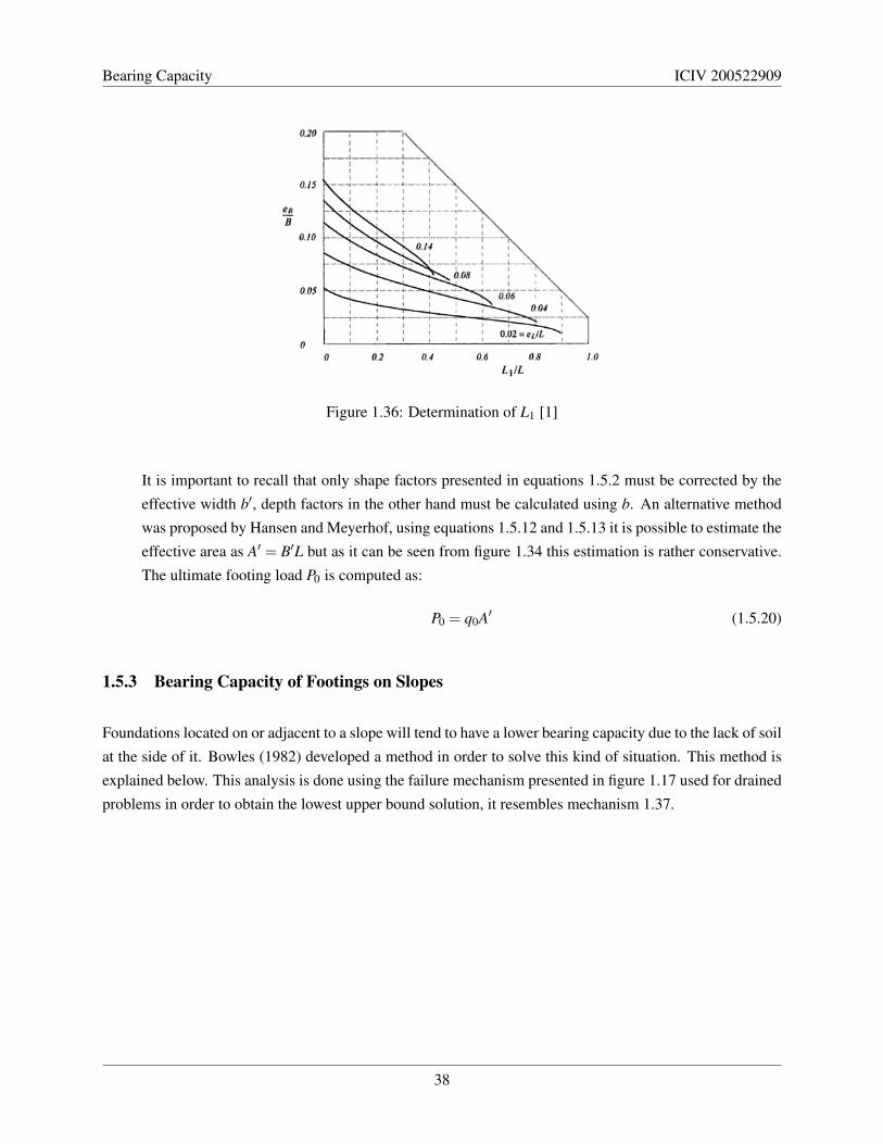
Highers and Anders in 1985 have suggested different plots and tables in order to calculate b1 and L1.

These plots are represented in figures 1.35 and 1.36[1].

Figure 1.35: Determination of b1 [1]

37


Figure 1.36: Determination of L1 [1]

It is important to recall that only shape factors presented in equations 1.5.2 must be corrected by the

effective width b′, depth factors in the other hand must be calculated using b. An alternative method

was proposed by Hansen and Meyerhof, using equations 1.5.12 and 1.5.13 it is possible to estimate the

effective area as A′ = B′L but as it can be seen from figure 1.34 this estimation is rather conservative.

The ultimate footing load P0 is computed as:

P0 = q0A′ (1.5.20)

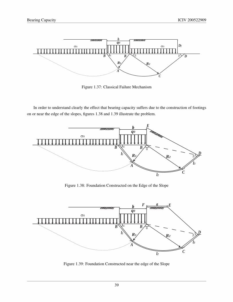
1.5.3 Bearing Capacity of Footings on Slopes

Foundations located on or adjacent to a slope will tend to have a lower bearing capacity due to the lack of soil

at the side of it. Bowles (1982) developed a method in order to solve this kind of situation. This method is

explained below. This analysis is done using the failure mechanism presented in figure 1.17 used for drained

problems in order to obtain the lowest upper bound solution, it resembles mechanism 1.37.

38


bq0

R1 R2

B D

σ0σ0

α β βB

AC

Df

Figure 1.37: Classical Failure Mechanism

In order to understand clearly the effect that bearing capacity suffers due to the construction of footings

on or near the edge of the slopes, figures 1.38 and 1.39 illustrate the problem.

bbq0

R1 R2

BD

σ0

α

β

l3

l1

l2 C

E

θB

A

Figure 1.38: Foundation Constructed on the Edge of the Slope

bbq0

R1 R2

BD

σ0

α

β

l3

l1

l2 C

E

θ

F a

B

A

Figure 1.39: Foundation Constructed near the edge of the Slope

39


Bowles [2] suggests that bearing capacity factors Nc and Nq must be corrected in order to compute an

improved result. These corrections are made using the following formulas:

N′c = NcLT

L0(1.5.21)

N′q = NqAT

A0(1.5.22)

Where N′c and N′q are the reduced bearing capacity factors used for the problem solution. LT is the total length

of the surface ABCD from figures 1.38 and 1.39 and L0 is the length of the surface from figure 1.37. AT is

the surcharge area framed by points BDE from figure 1.38 or BDEF from figure 1.39. A0 is the surcharge

area from fig 1.37 and is calculated as BDD f .

The total length from figures 1.38 and 1.39 can be easily calculated by the following procedures:

l1 =b2

cosα (1.5.23)

l2 can be calculated by an iterative process using the logarithm equation presented in equation 1.3.26.

li = cosυi(R2i+1−R2i) (1.5.24)

Where:

tanυi =sinθi+1R2i+1− sinθiR2i

cosθi+1R2i+1− cosθiR2i(1.5.25)

l3 =BD2

cosβ (1.5.26)

Regular values for α and β are π/4 + ϕ ′/2 and π/4− ϕ ′/2 respectively. Prior to these analysis some

considerations must be taken [15]:

• If AT > A0 then Nq is not corrected.

• The wedge factor Nγ is not corrected for slope effects.

• For ratios a/b > ( 1,5 or 2,0 ) there is no slope consideration, and the problem is treated in the classical

way.

40

Chapter 2

Constitutive Modeling in Soil Mechanics

2.1 Introduction

One of the main concerns in soil mechanics is to understand soil behavior. This encounters unlimited chal-

lenges in the moment of mathematically modeling such behavior. Constitutive modeling aims to describe

different aspects of soil, such as, shear strength, consolidation, deformations (elastic - plastic), stress states

and paths.[1]

Different models have been proposed using alternative implementations of mathematical formulae, and

even though some of them resemble in an accurate way different particular problems, most of them do not

describe in a complete way the material behavior. Therefore, it is important to understand fully the scope,

advantages and disadvantages of the model chosen. Some models are too simple to fully describe the material

behavior, while, others are too complex to understand the physical meaning of the parameters used in the

modeling.[13]

These models are formulated using critical state theories which have been broadly discussed in the aca-

demical field through the last decades. While in one verge some understand the critical state theory as a

unique and complete description of truth, the reluctant ones argue that critical state soil mechanics only

address particular problems, and since those models are not capable of reproducing all the features and phe-

nomenons observed in experimental analysis they conclude they do not have anything to offer. Such radical

opinions do not encourage a healthy discussion in whether or not critical state theory represents an accurate

approach to soil mechanics problems. This is why the scope of this document is developed under the same

tolerant framework cited by Wood [10] which is not about the relevance of its application but most impor-

tantly, it concerns the understanding of the topic, which may lead in the future to greater developments in

soil mechanics and to the possible improvement of these models flaws. This topic offers and insight of the

relevance of volume changes in soils and the influence they have in its behavior. Therefore, it is important

41

Constitutive Modeling in Soil Mechanics ICIV 200522909

to recall that despite constitutive modeling may fail to fully describe the soil behavior, the theoretical frame-

work in which it is supported must not be rejected nor neglected, since it provides evidence of the great

influence critical state theory offers in understanding soil mechanics.

2.2 Description

Constitutive modeling is a mathematical approach to describe how materials respond and behave when they

are submitted to stresses or strains.

All models are formulated using soil parameters and state variables. Soil parameters represent quantities

inherited from the material and even though they do not change due to processes of loading or unloading,

they can be altered due to chemical, biological or thermic processes. State variables represent the mechanical

conditions of a given material (Dynamical System) in a particular time.

Some models introduce different variables or parameters that do not have mechanical or physical mean-

ing so it is important to be well related with the mathematical approach used, in order to tackle the problem

and fully understand it.

The different formulae used to describe any constitutive model are know as constitutive equations. These

equations have the purpose of characterizing an individual material with relation to the applied loads (They

describe the macroscopic behavior resulting from the internal constitution of the material). [11] Constitutive

equations are not able to fully describe accurately a real material, instead they describe ideal material re-

sponses regarding experimental observations. Since material behavior is too complex to be fully described,

this is the best analytical approach that can be made in an effort to theoretically understand the soil behavior.

2.3 Implementation

The implementation of any model consists in mathematically describe and simulate a group of referenced

curves that may resemble the soil behavior. This document will present and explain the main features and as-

pects of Cam-clay, model developed at the University of Cambridge. The following chapters will address this

constitutive model, starting by understanding the principles of elastoplasticity and introducing the concepts

of yielding, plastic potential, strains (elastic - plastic), hardening law and the flow rule.

An element test is programmed for the modeling of a drained test using MATLAB and is presented in a

p′vs.q plot, using only the geometry of the model (No tensorial notation).

42

Chapter 3

Elasticity

3.1 Introduction

Elasticity is described by the unique relation in which strain depends only on the stress state of the material

and viceversa. The importance of this definition is to understand that strain or stress history is irrelevant in

the behavior of the material analyzed. The actual value of any of those (Strain - Stress) is enough to deter-

mine the other. This behavior is often known as "path-independent".

The main aspect of elasticity is that plastic deformations never occur, this means that any deformation the

material suffers is completely reversible. [8]

Mathematically the most common function to illustrate this behavior is the constitutive equation of

HOOKE, which in a uniaxial stress state is expressed as:

Txx = Eεxx (3.1.1)

Where Txx is the principal stress in the x direction, E is the Young Modulus and ε is the strain in the same

direction as the stress. In tensorial notation it is possible to understand the nature of the problem under the

following notation. The general constitutive equation for elastic behavior is expressed as:

T = C : ε (3.1.2)

Where T represents the effective CAUCHY stress tensor, C the fourth order stiffness tensor or tangent

modulus and ε the infinitesimal strain tensor.

43


3.2 Analyzing the Constitutive Equation

Elasticity is based under the assumption that the soil behaves isotropically, this means the soil is considered

as a material that exhibits the same properties in all directions. For this reason the components of the stiffness

tensor C are considered independent of the coordinated system chosen (Rectangular cartesian components

are unchanged by any orthogonal transformation of the coordinate axes[11]). Given the symmetry of the

tensor C:

Ci jkl = C jikl = Ci jlk (3.2.1)

It is possible to demonstrate that any isotropic tensor of fourth order can be represented through the lineal

combination of other three isotropic tensors. These tensors must be linearly independent. The procedure is

illustrated below.

Ci jkl = λAi jkl + µBi jkl +βDi jkl (3.2.2)

Where A, B, D are fourth order isotropic tensors and λ , µ and β are scalars. The three tensors depicted

before are defined as follows [9]:

Ai jkl = δi jδkl (3.2.3)

Bi jkl = δikδ jl (3.2.4)

Di jkl = δilδ jk (3.2.5)

Using expressions3.2.3, equation 3.2.2 can be rewritten into:

Ci jkl = λδi jδkl + µδikδ jl +βδilδ jk (3.2.6)

In order to simplify the expression 3.2.6 the following procedure is performed.

Ci jkl−C jikl = λδi jδkl + µδikδ jl +βδilδ jk−λδ jiδkl + µδ jkδil +βδ jlδik

Factorizing terms:

Ci jkl−C jikl = λδkl(δi j−δ ji)+ µ(δikδ jl−δ jkδil)+β (δilδ jk−δ jlδik)

= µ(δikδ jl−δ jkδil)+β (δilδ jk−δ jlδik)

δikδ jl(µ−β ) = (β −µ)δilδ jk

44


Simplifying Kronecher-Delta δi j when i = j.

δ jkδ jl(µ−β ) = δ jlδ jk(β −µ)

(µ−β ) = (β −µ)(

δ jlδ jk

δ jkδ jl

)(µ−β ) = (β −µ)

2µ = 2β ⇒ µ = β

(3.2.7)

From expression 3.2.7, equation 3.2.6 can be simplified into:

Ci jkl = λδi jδkl + µ(δikδ jl +δilδ jk) (3.2.8)

Expression 3.2.8 can be simplified further introducing the unit isotropic fourth order tensor I defined as:

Ii jkl =12

δikδ jl +δilδ jk (3.2.9)

And since:

δmnδop = 1mnop = 1⊗1 (3.2.10)

Equation 3.2.8 is altered into:

C = Ce = λ1⊗1+2µI (3.2.11)

Where Ce is defined as the stiffness tensor for the elastic model, and λ and µ are defined as the LAME’S

coefficients. The tangent modulus Ce can be interpreted also in terms of volumetric and deviator tensors.

These tensors are defined in equations 3.2.12 and represent the decomposition of the unit isotropic tensor I.

Ivol =13

1⊗1 (3.2.12)

Idev = I− 13

1⊗1 (3.2.13)

Equation 3.2.11 can be rewritten in terms of tensors 3.2.12 following the procedure illustrated below.

Ce = λ1⊗1+2µI

=33

λ1⊗1+2µ

(Ivol + Idev

)= 3λ Ivol +2µIdev

= (3λ +2µ)Ivol +2µIdev

(3.2.14)

Now that tensor Ce has been defined it is possible to compute the inverse tensor C−1e which is of main

interest, since for many problems the stress state is known and strains can be computed easily by using this

tensor.

ε = T : C−1e (3.2.15)

45


The following properties must be satisfied for I, since it is known to be a unit symmetrical fourth order

tensor.

Ivol : Ivol = Ivol (3.2.16)

Idev : Idev = Idev (3.2.17)

Ivol : Idev = Idev : Ivol = 0 (3.2.18)

Ivol + Idev = I (3.2.19)

I = Ce : C−1e (3.2.20)

Tensor C−1e can be defined by a linear independent combination of a volumetric and deviator part such as:

C−1e = β1Ivol +β2Ivol (3.2.21)

Now from properties 3.2.16 it is possible to compute an expression for C−1e:

Ce : C−1e = I = [(3λ +2µ)Ivol +2µIdev] : [β1Ivol +β2Ivol] (3.2.22)

Where β1 and β2 must have the following values in order to satisfy the identity principle:

β1 =1

3λ +2µ(3.2.23)

β2 =1

2µ(3.2.24)

Finally equation 3.2.21 can be formulated as:

C−1e =1

3λ +2µIvol +

12µ

Idev (3.2.25)

The previous mathematical notation has been presented in terms of the LAME’S coefficients, however,

alternative notations exist in the literature using material parameters known as the Young modulus E and the

Poisson ratio defined as ν . While the LAME’S constants constitute a purely mathematical and theoretical

definition, E and ν have a more physical meaning and are commonly used in constitutive models. The

relation between the elastic constants E, ν and the coefficients λ and µ is explained in the following section.

46


3.3 Model Parameters

For an elastic material, the Cauchy tensor is defined by index notation as:

Ti j = Ci jklεkl

= λδi jδkl +2µ12(δikδ jl +δilδ jk)εkl

= λεkkδi j +2µ12(δikδ jl +δilδ jk)εkl

= λeδi j +2µεi j

(3.3.1)

Or in tensorial notation as:

T = λeI+2µε (3.3.2)

Where εkk (Einstein Notation) is known as the first invariant and is mathematically computed as e = tra(ε).The components of the symmetric tensor T are given by[19]:

T11 = λ (ε11 + ε22 + ε33)+2µε11 (3.3.3)

T22 = λ (ε11 + ε22 + ε33)+2µε22 (3.3.4)

T33 = λ (ε11 + ε22 + ε33)+2µε33 (3.3.5)

T12 = 2µε12 (3.3.6)

T13 = 2µε13 (3.3.7)

T23 = 2µε23 (3.3.8)

Equations 3.3.3 are known as the constitutive equations for a lineal, elastic and isotropic material. Applying

the Einstein notation for Tkk and solving for e is possible to find the value of the total volumetric strain.

Tkk = (3λ +2µ)εkk = (3λ +2µ)e (3.3.9)

e =Tkk

3λ +2µ(3.3.10)

An alternative approach to the previous solution can be made using the inverse tensor equation 3.2.25.

ε = [1

3λ +2µIvol +

12µ

Idev] : Ivol : T (3.3.11)

ε =1

3λ +2µIvol : T (3.3.12)

εi j =1

3λ +2µ

(13

Tkkδi j

)(3.3.13)

Then:

tr(ε) = e =1

3λ +2µTkk

47


As it was proven previously by expression 3.3.11. Now, it is possible to solve equation 3.3.1 solving for εi j

and replacing expression 3.3.11 for e.

εi j =1

2µTi j−

λ

2µeδi j

=1

2µ(Ti j−λeδi j)

=1

2µ

(Ti j−

λ

3λ +2µTkkδi j

) (3.3.14)

A uniaxial stress state is defined by the following notation:

T11 6= 0 and for any other component Ti j = 0

The individual components of tensor ε for a uniaxial state are:

ε11 =1

2µ

[T11−

λ

2µ +3λT11

]=

λ + µ

µ(3λ +2µ)T11 (3.3.15)

ε22 = ε33 =− λ

2µ(2µ +3λ )T11 =− λ

2(λ + µ)ε11 (3.3.16)

ε12 = ε13 = ε23 = 0 (3.3.17)

YOUNG’S elasticity modulus is defined as E = σ/ε , which is tonsorially equivalent to E = T11/ε11.

E =µ(3λ +2µ)

λ + µ(3.3.18)

Finally the strains of the principal axis are related and the POISSON’S ratio is computed by the following

expression. Since, ε11/ε22 = ε11ε33.

ν =λ

2(λ + µ)(3.3.19)

The equations relating the LAME’S coefficients and the elastic constants E and ν are:

µ =E

2(1+ν)(3.3.20)

λ =νE

(1+ν)(1−2ν)(3.3.21)

With these values tensor T can be formulated as:

T =[

νE(1+ν)(1−2ν)

1⊗1+E

1+νI]

: ε (3.3.22)

=νE

(1+ν)(1−2ν)eI+

E1+ν

ε (3.3.23)

48


And 3.3.14 can be expressed as:

εi j =1E

[(1+ν)Ti j−νsδi j] (3.3.24)

Where s is defined as Tkk = tr(T). Using volumetric and deviatoric notation expressions 3.3.22 can be

rewritten as:

T =[

νE(1+ν)(1−2ν)

Ivol +E

1+νIdev]

: ε (3.3.25)

Finally, it is important to introduce two more parameters which are commonly used in soil mechanics. If

only one pair of shear stresses are not zero, this is known as a simple shear stress state. This means T12 = T21

and from equations 3.3.3:

ε12 = ε21 =T12

2µ(3.3.26)

The Shear Modulus G′ is defined as the ratio of the shearing stress (T12 = T21 = τ) in simple shear, to the

shear strain. Then, the shear modulus G′ is mathematically computed as:

G′ ≡ τ

2ε12=

T12

2ε12=

µ��2ε12

��2ε12(3.3.27)

From expression 3.3.27 is possible to conclude that LAME’S constant µ corresponds to the magnitude of

the shear modulus G′.[9]

G′ = µ :=E

2(1+ν)(3.3.28)

The second parameter is known as the Bulk Modulus K′ and represents the resistance to volume change. It is

expressed as the ratio of hydrostatic pressure to the unit change in volume. This resultant hydrostatic stress

is isotropic and is expressed as (Volumetric Part) :

T = K′e1 = 3K′Ivolε (3.3.29)

Then, using equation 3.3.2 and since ε11 = ε22 = ε33 = e/3:

K′ =λe+2µεii

e

= λ +2µ

3

=E

3(1−2ν)

(3.3.30)

Using the shear modulus G′ and the bulk modulus K′, equation 3.3.22 can be finally computed as:

T =[(

K′− 23

G′)

1⊗1+2G′I]

: ε (3.3.31)

49


Equation 3.3.32 can be simplified using expression 3.3.29, and since, G′ = µ:

T =(

3K′Ivol +2G′Idev)

: ε (3.3.32)

50

Chapter 4

Elastoplasticity

4.1 Introduction

The behavior of soil is too complex in contrast to other materials, such as, metals. This is why different

idealizations have been made to describe the plastic behavior of soils.

In order to predict the behavior of any structure when plastic deformations occur, the first step is to choose an

appropriate idealization mechanism that resembles the structure behavior. Basically an elastoplastic model

refers to an idealization in which the material analyzed is supposed to behave inside an elastic domain until

yielding. For this scenario elastic deformations occur until the yielding surface is reached and plastic strains

increments take place after initial yielding. Since any stress state can be reached by an endless number of

stress paths, the behavior in soil mechanics can not be longer understood by a single relation of stresses and

strains. This means that contrary to other materials, in soil mechanics, the loading path is totally different to

the unloading trajectory followed when the load is retired. In order to fully describe the stress-strain relations

for an elastoplastic material, the following concepts must be introduced and satisfied.

1. A Yield Function must be defined (State Boundary Surface).

2. A relationship between the directions of the principal plastic strain increments and the principal

stresses is required.

3. A hardening law for the material must be given. This relates the amount the material hardens and the

plastic strain it undergoes.

4. A flow rule must be established. This specifies the relative magnitudes of the incremental plastic

strains when the material is yielding.

51

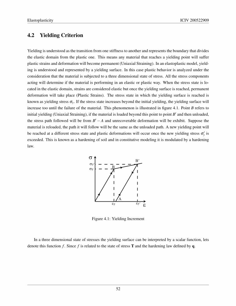
Elastoplasticity ICIV 200522909

4.2 Yielding Criterion

Yielding is understood as the transition from one stiffness to another and represents the boundary that divides

the elastic domain from the plastic one. This means any material that reaches a yielding point will suffer

plastic strains and deformation will become permanent (Uniaxial Straining). In an elastoplastic model, yield-

ing is understood and represented by a yielding surface. In this case plastic behavior is analyzed under the

consideration that the material is subjected to a three dimensional state of stress. All the stress components

acting will determine if the material is performing in an elastic or plastic way. When the stress state is lo-

cated in the elastic domain, strains are considered elastic but once the yielding surface is reached, permanent

deformation will take place (Plastic Strains). The stress state in which the yielding surface is reached is

known as yielding stress σy. If the stress state increases beyond the initial yielding, the yielding surface will

increase too until the failure of the material. This phenomenon is illustrated in figure 4.1. Point B refers to

initial yielding (Uniaxial Straining), if the material is loaded beyond this point to point B′ and then unloaded,

the stress path followed will be from B′−A and unrecoverable deformation will be exhibit. Suppose the

material is reloaded, the path it will follow will be the same as the unloaded path. A new yielding point will

be reached at a different stress state and plastic deformations will occur once the new yielding stress σ ′y is

exceeded. This is known as a hardening of soil and in constitutive modeling it is modulated by a hardening

law.

σ

ε

Β

εy

σy

Α

Β’

εy’

σy’

Figure 4.1: Yielding Increment

In a three dimensional state of stresses the yielding surface can be interpreted by a scalar function, lets

denote this function f . Since f is related to the state of stress T and the hardening law defined by q.

52


The yielding criterion will be understood by the following criteria:

f (T,q) < 0 (Material Behaves Elastically) (4.2.1a)

f (T,q) = 0 (Yielding Reached. Plastic Deformations Occurred) (4.2.1b)

f (T,q) > 0 (Impossible State of Stresses) (4.2.1c)

Since f increases proportional to the state of stresses T once the initial yielding surface is reached, it is clear

that any stress state can not be located outside the yielding surface boundary, then f (T,q) > 0 represents an

impossible stress state T.

4.3 Strains

Deformations are the result of different stresses states produced by thermic, mechanical or chemical pro-

cesses. In mathematical notation the strain tensor ε in elastoplasticity is defined by the composition of an

elastic deformation and a plastic strain.

ε := εe + ε

p (4.3.1)

Altering equation 3.1.2 into:

T = C : (ε− εp) (4.3.2a)

T = C : (D−Dp) (4.3.2b)

Where T is the effective stress rate and D the strain rate. The superscripts e and p describe elastic and plastic

behavior respectively.

53


4.3.1 Elastic Strains

Directions of principal strain increments coincide with directions of the principal stress increments.[10]

σ1 σ1

σ2

σ2

σ1 σ1

σ2

σ2

δτ

δτ

δτ

δτ

Figure 4.2: Elastic Behavior

Any stress state located in the elastic domain causes elastic deformations. Elastic strains are decomposed

into volumetric strains εep and shear strains εe

q . This means strains are influenced by a volumetric stress and

a deviator stress. Volumetric stress is defined by p′ and represents the effective mean stress.

p′ =σ ′1 +σ ′2 +σ ′3

3(4.3.3)

The deviator stress is defined as:

q′ =1√2

√(σ ′1−σ ′2)2 +(σ ′2−σ ′3)2 +(σ ′3−σ ′1)2 (4.3.4)

Since water has no shear strength the deviator stress can be expressed in terms of total or effective stresses

without altering the result.

• Axisymmetric Stress Conditions:Analyzing an axisymmetric stress condition such as a triaxial test (σ ′2 = σ ′3), equations 4.3.3 and 4.3.4

can be expressed in the following way:

p′ =σ ′1 +2σ ′3

3(4.3.5)

q′ = σ′1−σ

′3 (4.3.6)

54


Solving for σ ′a and σr.

σ′a = p′+

2q3

(4.3.7)

σr = p′−q/3 (4.3.8)

The infinitesimal elastic deformations for the axial and radial strain are defined using equation 3.3.24

defined in the previous chapter.

δεa =1E

(δσ′a−2δσ

′rν) (4.3.9)

δεr =1E

(−νδσ′a− (1−ν)δσ

′r) (4.3.10)

The elastic constants E and ν are used since elastic deformations are being described. Corresponding

to the stress parameters p′ and q, deformations can also be interpreted in terms of volumetric strains

and deviator strains. Volumetric strains will be denoted as εep and deviator strains as εe

q . Where

the superscript represents elastic behavior and the subindex whether the deformation is caused by a

volumetric or deviator strain.

δεe = δε

ep +δε

eq (4.3.11)

εep = εa +2εr (4.3.12)

εeq =

23(εa + εr) (4.3.13)

In constitutive modeling it is usually worked in terms of strains increments:

δεep = δεa +2δεr (4.3.14)

δεeq =

23(δεa +δεr) (4.3.15)

The factor 23 is used in expressions 4.3.11 and 4.3.14 of the shear strain εe

q in order to satisfy the

evaluation of work done by deformations, defined as:

p′δεeq +qδε

ep = σ

′aεa−2σ

′rεr (4.3.16)

In order to relate equations 4.3.11 and 4.3.14 with the stress parameters q′ and p′, equations 4.3.7 are

replaced into 4.3.9 and finally computed in 4.3.14.

δεep =

1E

(3δ p′−6νδ p′) (4.3.17)

δεeq =

1E

(2ν

3δq+

23

δq)

(4.3.18)

55


It is possible to simplify expressions 4.3.17 into:

δεep =

[3(1−2ν)

E

]δ p′ (4.3.19)

δεeq =

[2(1+ν)

3E

]δq (4.3.20)

Recalling the Bulk 3.3.30 and Shear Modulus 3.3.28 defined in the previous chapter expression 4.3.21

is simplified into:

δεep =

1K′

δ p′ (4.3.21)

δεeq =

13G′

δq (4.3.22)

Where:

K′ =E

3(1−2ν)

G′ =E

2(1+ν)

Since elastic strain was defined previously as 4.3.11:

δεe = δε

ep +δε

eq

It is possible to rewrite it as:

δεe =

1K′

δ p′+1

3G′δq (4.3.23)

• Isotropic Compression (Swelling and Recompression):Volume - pressure relations are usually understood in soil mechanics as p′vs.V plots 4.3.

p’

v

Figure 4.3: Isotropic Compression

56


In critical state theory these plots are assumed to be straight in ln(p′)vs.V 4.4, where λ is the slope of

the virgin compression line commonly addressed as the normal compression line (N.C.L), and κ is the

slope of the swelling and recompression lines.

ln (p’/p0’)

λ

κ

N

N.C.L

pc’

vo

v

Δvp

p’1

A

BC

κ

vkvf

vcΔve

Δv

Figure 4.4: Idealized Compression Behavior

Soil from figure 4.4 is loaded from point A until a pre-consolidation stress defined as p′c. Then it is

unloaded to point C, and as it can be observed, different paths are followed through the virgin com-

pression line, and the swelling-recompression lines. This means, even though some deformations are

recovered after unloading, soil exhibits permanent deformations εp.

In short, once the pre-consolidation stress is reached plastic deformations may occur.

57


4.3.2 Plastic Strains

In plastic behavior directions of the principal strain increments coincide with the directions of the

principal stresses.[10]

σ1 σ1

σ2

σ2

σ1 σ1

σ2

σ2

δτ

δτ

δτ

δτ

Figure 4.5: Plastic Behavior

The equation of the normal consolidation line (N.C.L) is:

v = N−λ ln(p′) (4.3.24)

v = vλ −λ ln(p′) (4.3.25)

Where N is the specific volume for 1 mean pressure unit in the virgin compression line. N is a constant

for a particular soil and is often refereed as a vλ line. The equation of a swelling-recompression line

is:

v = vκ −κln(p′) (4.3.26)

Similarly as N, vκ is the specific volume for 1 mean pressure unit in a swelling-recompression line. vκ

depends on which swelling-recompression line the soil is.

From figure 4.4:

∆vp = v0− v f (4.3.27)

Then, replacing v0 and v f into 4.3.27 :

v0 = vc−λ ln(p′cp′

)

v f = vc−κln(p′cp′

)

∆vp =��vc−λ ln(p′cp′

)−��vc +κln(p′cp′

)

∆vp = (κ−λ )ln(p′cp′

)

(4.3.28)

58


Finally it is possible to define the plastic strain due to stress and state.

δεpp =

δvp

v

= (κ−λ )ln(p′cvp′

)

As well as elastic strains, shear deformations are analyzed in terms of volumetric and deviator strains

by εpp and ε

pq respectively. ε

pq is calculated from the flow rule of the model chosen.

δεp = ε

pp + ε

pq (4.3.29)

δεpp α

δ fδ p′

= (κ−λ )ln(p′cvp′

) (4.3.30)

δεpq α

δ fδq

:=δε

pp

δεpq

(CAM-CLAY) (4.3.31)

Where f is defined as the stress state function of equilibrium (Yielding Function). α denotes propor-

tionality.

4.4 Plastic Potential

The potential function is used to describe a vector quantity with relation to a specific point in space. It is a

scalar function of position, so it is possible to determine a unique defined direction by calculating its partial

derivatives. The plastic potential is defined by g(σa,σb,σc) = 0 and depicts a surface in the principal stress

space. Strain increment vectors are normal to the potential surface (Stress Space). By this principle it is

possible to formulate an equation that describes the plastic strain increment (see Equation 4.3.29).

δεp = δm

δgδσ

(4.4.1)

Where δm is defined as the plastic multiplier (also referred as δλ in the literature) and g denotes the plastic

potential. Figure 4.6 describes this behavior.

59


p'

q

δε(p,q)

δε(p,p)

δεp

Plastic Potential

Strain Increment

Figure 4.6: Plastic Potential

The plastic potential function for a material can be determined by performing careful and detailed ex-

periments. In some scenarios, such as, metals, the plastic potential coincides with the yielding surface f .

The condition q = f satisfies the principle of normality, which represents the scenario when the plastic strain

increments are normal to the yield locus (Normal to any point of the yielding surface). The condition of

normality is often referred as an associated flow. [10]

4.5 Hardening Law

Figure 4.7 represents the the easiest way to introduce the concept of strain hardening. This means that after

the material yields, the stress- strain curve remains liner but its slope is reduced.

σ

ε

Figure 4.7: Idealization: Strain-Hardening

60


This idealization is only used to introduce the concept of Strain-Hardening, in soil mechanics a more

complex mechanism should be chosen.

The hardening law generalizes the concept of uniaxial stress conditions depicted in figure 4.7 into general

stress states. Hardening a material can result in two different kinds of behaviors of the yield surface.

• Isotropic Hardening: The yielding surface is enlarged in the stress space.

• Kinematic Hardening: The yielding surface is translated from its inial point.

Figure 4.8 describes both types of hardening.

p'

q

p'

q

Isotropic Hardening Kinematic Hardening

δσ

δσ

Figure 4.8: Hardening

The most commonly mechanism used mechanism to describe material hardening is isotropic-hardening,

since it offers simpler relations to mathematically describe the material behavior. In reality this behavior is

sometimes unrealistic, and kinematic hardening offers a suitable description. Under monotonic loading the

isotropic-hardening is often adequate. The hardening law influences the yield surface equation used in the

constitutive model (This concept was introduced in the yielding criterion).

f (T,q) = 0

Where q is a vector of hardening parameters. These parameters will define the size of the yield locus and

will be related to the components of the plastic strain (volumetric-deviator).[10]

61


4.6 Flow Rule

The flow rule determines the ratios of the plastic strains increments once the material has yielded in a par-

ticular stress state. A flow rule simply describes the relative sizes of individual strain increments, it does not

define the absolute size of the plastic deformation. The flow rule is defined by equation 4.4.1.

δεp = δm

δgδσ

Which can be rewritten into equation 4.6.1 if the flow rule is associative.

δεp = δm

δ fδσ

(4.6.1)

In tensorial notation the flow rule is described by a unit flow rule tensor B and the increment of the plastic

strain is defined by:

Dp = γB(T,q) (4.6.2)

Where γ is the consistency parameter and Dp is the rate of plastic strains. Introducing a new concept which

is the consistency condition. It can be understood as the requirement for the load point to remain on the yield

surface during plastic deformations (Time-independent plasticity).[4] In order to evaluate the consistency

parameter γ it is necessary to introduce and satisfy the Kuhn-Tucker conditions.[7]

γ ≥ 0 (4.6.3)

f (T,q)≤ 0 (4.6.4)

γ f (T,q) = 0 (4.6.5)

γ f (T,q) = 0 (4.6.6)

These conditions determine the model behavior by limiting any stress state to the yielding boundary and the

consistency condition.

62


4.7 Stiffness Modulus

As well as it was explained in chapter 3, it is possible to relate the stress tensor T with the strain ε by

a stiffness modulus which in this case will be defined as Cep. The equation is derived as follows using

equation 4.6.2:

f =∂ f∂T

: T+∂ f∂q

q (4.7.1)

=∂ f∂T

: Ce : (D−Dp)+∂ f∂q

q (4.7.2)

=∂ f∂T

: Ce : D− γ

[∂ f∂T

: Ce : B− ∂ f∂q

qγ

](4.7.3)

Solving the equation for f (T,q)) = 0 and satisfying the consistency requirement explained in subsection

4.6 and expressions 4.6.3, it is possible to conclude γ ≥ 0. Now it is possible to express γ by the following

implicit equation:

γ =∂ f∂T : Ce : D

∂ f∂T : Ce : B− ∂ f

∂qqγ

(4.7.4)

Using equations 4.3.2 and 4.6.2 is possible to formulate T as:

T = Ce : (D−Dp)

= Ce : (D− γB)Cep : D(4.7.5)

Replacing equation 4.7.4 into 4.7.5:

Cep = Ce−Ce : B⊗ ∂ f

∂T : Ce

∂ f∂T : Ce : B− ∂ f

∂qqγ

(4.7.6)

In order to simplify the previous equation, the denominator is defined as χ and the derivative tensor ∂ f∂T is

referred as N. The elastoplastic modulus is finally defined as [7]:

Cep = Ce−Ce : B⊗N : Ce

χ(4.7.7)

63

Chapter 5

Cam-Clay

5.1 Introduction

Cam Clay is the first critical state model developed to describe the behavior of soft soils, such as, clays. It

was formulated by Cambridge University researchers (Roscoe) and even though in present time it does not

offer an accurate description to fully describe the soil behavior, it constitutes an important contribution to

soil mechanics.[16] The main aspects which describe Cam Clay are:

• Strain-Stress relations. (Elastoplastic idealization)

• Volume and stress relations q. (Compression and Dilatancy)

• Critical state theory.

Cam Clay is modeled under axisymmetric stress conditions (see subsection 4.3.1) such as, triaxial tests and

is formulated under the following assumptions:

• The soil behavior is elastoplastic.

• The soil behaves and deforms as a continuum.

• The soil behavior is not affected by creep (Volume Change under constant effective stress).

• The soil is isotropic.

The former model was enhanced by Roscoe and Burland in 1968 and is known as the Modified Cam

Clay. The following sections describe both models, their scope, and formulations.

64

CamClay ICIV 200522909

5.2 Critical State Theory

The critical state concept is defined as the condition under unlimited deformations occur under a constant

state of effective stress and constant volume. The dilatancy angle ϑ is equal to zero. Mathematically it can

be expressed as:∂ p′

∂εq=

∂q′

∂εq=

∂v∂εq

= 0 (5.2.1)

From experimental analysis it has been observed that different stress states form a surface that can be plotted

as a line in the planes p′,v.

ln p’

λ

κ

N

λ

Γ

C.S.LN.C.L

pc’pc’/2

vκ

v

Figure 5.1: Critical State Line

This line is known as the Critical State Line (C.S.L) and is parallel to the virgin compression line (N.C.L).

The equations characterizing this line in space are:

q′ = Mp′ (5.2.2)

v = Γ−λ ln(p′) (5.2.3)

Where Γ is the specific volume to one unit pressure in the C.S.L and M is its slope in a p,q plot. The normal

consolidation line was already defined in section 4.3.2 and is described by equation 4.3.24:

v = N−λ ln(p′)

v = vλ −λ ln(p′)

65


If at some point the load is retired, it will follow an unloading -reloading path. The equation for a swelling -

recompression line is given by equation 4.3.26.

v = vκ −κln(p′)

The following consideration must be clarified to illustrate the concept of the critical state line:

Stress states located on the N.C.L are normally consolidated. A soil which lays at the left side of the C.S.L

is considered highly overconsolidated and the behavior of the soil at the right side is much similar as the

one of a lightly overconsolidated soil.[6]

5.3 Parameters

The critical state parameters are defined by p′, q and v which describe the soil behavior in a triaxial test. This

is why the same conditions explained for Axisymmetric stress conditions apply for this modeling.

p′ =σ ′1 +2σ ′3

3q′ = σ

′1−σ

′3

v = 1+ e

It is important to recognize the importance of path dependance in soil mechanics (Different types of tests

lead to different stress paths, as well as, different deformations). This is why tensorial notation is commonly

used in critical state models in order to describe any kind of path followed. The model constants are M, Γ,

κ , λ which characterizes the soil sampled.

5.4 Yielding Surface Evolution (Flow Rule)

Cam Clay is depicted by a yielding boundary reached by the following equation when the deviator stress q

is equal to (Three dimensional space):

q =Mp′

(λ −κ)(Γ−λ − v−λ (p′)) (5.4.1)

66


The yielding point is reached when the pre consolidation state of stress is reached, this means, the point

will lie on the Stable State Boundary Surface (S.S.B.S) and the unloading-reloading line (κ line). The

S.S.B.S is defined as:

vλ = Γ+(λ −κ)(1− η

M) (5.4.2)

Where η is the parameters ratio q/p′. The yield locus which defines the yielding surface is deduced by the

strain plastic rate:δε

pp

δεpq

= M− qp′

(5.4.3)

From the condition of normality (Associative Rule):

δεpp

δεpq· δq

δ p′=−1 (5.4.4)

Replacing δqδ p′ from expression 5.4.4 into equation 5.4.3:

δqδ p′

=qp′−M (5.4.5)

Finally equation 5.4.5 is integrated, and using the mathematical relation 5.4.6 it is possible to obtain the yield

locus defined as equation 5.4.7:dη

d p′=

p′ dqd p′ −q

p′2(5.4.6)

q = Mp′ln(p′cp′

) (5.4.7)

Where p′c is the preconsolidated mean stress. It is important to recall that elastic straining is governed by

the κ line equation. Modified Cam-Clay is governed by the same postulates as the classical model, but the

yielding surface is fitted by an elliptical scalar function defined as:

q2 +M2 p′2 = M2 p′p′c (5.4.8)

The principal distinction from this model and the classical Cam-Clay is the assumption for dissipated energy.

Modified Cam-Clay assumes dissipated energy as:

p′δεpp +qδε

pq = p′

√(δε

pp )2 +M2(δε

pq )2 (5.4.9)

Resulting in the flow rule:δε

pp

δεpq

=M2−η2

2η(5.4.10)

Strains for both models are calculated under the description given in the previous chapters taking under

consideration the respective flow rule used for each model.

67


Remarks:

• The effective stress path for a Drained test is equal to the total Stress path as a result of volumetric

change.

• An Undrained test does not exhibit volumetric change, Therefore, the mean stress p′ is supposed

constant until reaching the yielding surface. Once the yielding locus is reached volumetric and deviator

strains take place and are equal and opposite to direction to the other.

5.5 Hardening Rule

The evolution of the yield surface once the yielding locus is reached is described by the partial derivatives of

the yielding locus with relation to the volumetric and deviator strains:

δ p′c =∂ p′c∂ε

pp

δεpp +

∂ p′c∂ε

pq

δεpq (5.5.1)

Remarks:

• The yielding surface evolution only applies for lightly and normally consolidated soils.

• If the soil is highly overconsolidated the initial yielding surface remains constant.

5.6 Consolidation

This section presents the modulation of different behaviors of clays under undrained conditions considering

a Normally Consolidated 5.2, Slightly Overconsolidated 5.3and Highly Overconsolidated soil 5.4. The al-

gorithm of the model is included in the appendix of the work. The parameters used as input of the model

are:

λ = 0.22

κ = 0.011

e = 1

M = 1.2

p′c = 200kPa

P′0 = 200kPa = 170kPa = 30kPa

68


Figure 5.2: Normally Consolidated

Figure 5.3: Slightly Overconsolidated

69


Figure 5.4: Highly Overconsolidated

70

Chapter 6

Appendix

6.1 MATLAB Algorithm (Drained Test)

The following algorithm describes the explicit implementation of the Modified Cam-Clay model. All text

written in italic represents comments of the procedure.

function[]=CamClayDrained;

Input Parameters

fprintf (’Initial Conditions of the Test and Material Parameters:’);

G=input(’Shear Modulus (kPa):’);

Lambda=input(’λ :’);

Kappa=input (’κ :’);

e0=input (’Initial Void Ratio:’);

M=input(’M:’);

SigmaV=input (’p′v (kPa):’);

Isotropic Normally Consolidated

Pinicial= input (’p′0 (kPa):’);

Consolidation State of the Soil. 1.Normally Consolidated. 2. Overconsolidated.

Initial Specific Volume

v0=1+e0;

Soil Overconsolidated

if Pinicial<2/3*SigmaV;

Pv=2/3*SigmaV;

if Pinicial<1/3*Pv

71


Ec=2;

Highly Overconsolidated

sc=1;

else

Ec=1;

Slightly Overconsolidated

sc=1;

end

Soil Normally Consolidated

else

Ec=1;

Pv=Pinicial;

end

Initial Conditions and Yielding Point

a = 9+M2;

b =−M2 ∗Pv−18∗Pinicial;

c = 9∗Pinicial2;

p = (−b+ sqrt(b2−4∗a∗ c))/(2∗a);Mean Effective Stress

q = 3∗ (p−Pinicial);Specific Volume Calculation

vp0 = v0−Kappa∗ log(Pv/Pinicial);

Coordinated Intersection Points CSL - TSL

q f = (3∗M)∗Pinicial/(3−M);p f = Pinicial +q f /3;

Increment from the intersection point CSL - TSL to the Yielding Point.

intervalo=1000;

dq = (q f −q)/intervalo;

Total Stress Path = Effective Stress Path

Increment dq until yielding point.

qi(1) = 0;

pi(1) = Pinicial;

72


vc(1) = 0;

vi(1) = v0;

for i=2:+1:intervalo+1

if i==2

qi(i)=q;

pi(i)=qi(i)/3 + Pinicial;

else

qi(i)=qi(i-1)+dq;

pi(i)=qi(i)/3 + Pinicial;

end

p0c(i) = (qi(i)2 +(M2 ∗ pi(i)2))/(M2 ∗ pi(i));

Specific Volume

vp0c(i) = vp0−Lambda∗ log(p0c(i)/Pv);vc(i) = vp0c(i)+Kappa∗ log(p0c(i)/pi(i));vi(i) = vc(i);end

Elastic volumetric and shear increment.

dEeq(1) = dq/(3∗G);dEep(1) = (Kappa∗ (pi(1)− p))/(vp0∗ p);dE p(1) = (vp0− vc(1))/vp0;

dE pp(1) = dE p(1)−dEep(1);dE pq(1) = (qi(1))/(M2 ∗ (pi(1)− p0c(1)/2))∗dE pp(1);dEq(1) = dEeq(1)+dE pq(1);eq(1) = dEq(1);ep(1) = dE p(1);epsilon(1) = 0;

for i=2:+1:intervalo+1

dEep(i) = Kappa∗ (pi(i)− p)/(vp0∗ p);dEeq(i) = dq/(3∗G);Total Volumetric Strain Increment

dE p(i) = (vp0− vc(i))/vp0;

Plastic Volumetric Strain

dE pp(i) = dE p(i)−dEep(i);Shear Plastic Strain Increment

dE pq(i) = (dE pp(i)∗qi(i))/(M2 ∗ (pi(i)− p0c(i)/2));

73


Total Shear Strain Increment

dEq(i) = dEeq(i)+dE pq(i);eq(i) = eq(i−1)+dEq(i);Total Volumetric Strain Increment

dE p(i) = dEep(i)+dE pp(i);ep(i) = ep(i−1)+dE p(i);epsilon(i) = (3∗ eq(i)+ ep(i))/3;

end

eq(i) = eq(i−3);

Initial Yielding Surface

Dp f i = Pv/intervalo;

p f i(1) = 0;

q f i(1) = 0;

f ori = 2 : +1 : intervalo+1

p f i(i) = p f i(i−1)+Dp f i;

Yielding Scalar Function

q f i(i) = sqrt((M2)∗ (p f i(i)∗ (Pv− p f i(i))));end

Final Yielding Surface

Normally or Slightly Consolidated Soils.

i f Ec == 1

Dp f f = p0c(intervalo+1)/intervalo;

p f f (1) = 0;

q f f (1) = 0;

f ori = 2 : +1 : intervalo+1

p f f (i) = p f f (i−1)+Dp f f ;

q f f (i) = sqrt((M2)∗ (p f f (i)∗ (p0c(intervalo+1)− p f f (i))));end

Highly Overconsolidated soil: It is not necessary to calculate a new Yielding Surface

elseif Ec==2

p f f (1) = 0;

q f f (1) = 0;

end

74


Critical state line

f ori = 1 : +1 : intervalo pcs(i) = p f i(i);qcs(i) = M ∗ pcs(i);end

pcs(i+1) = p f +20;

qcs(i+1) = M ∗ pcs(i+1);

Plot 1

subplot(2,2,1),plot(pi,qi,pcs,qcs,pfi,qfi,pff,qff),title(’Cam Clay’),xlabel(’p´[kPa]’),ylabel(’q [kPa]’);

Plot 2

subplot(2,2,2),plot(eq/1000,qi),title(’eq vs. q’),xlabel(’eq’),ylabel(’q [kPa]’);

Plot 3

subplot(2,2,3),plot(log(pi),vi),title(’Log(p) vs. v’),xlabel(’log(p)’),ylabel(’v’);

Plot 4

subplot(2,2,4),plot(eq/1000,vi),title(’eq vs. v’),xlabel(’eq’),ylabel(’v’);

75

Bibliography

[1] F. Azizi. Applied Analyses in Geotechnics. Taylor and Francis Group, 2006.

[2] J.E Bowles. Foundation Analysis and Design. McGraw-Hill International Book Company, 1984.

[3] W. Chen. Limit analysis and soil plasticity, 2007.

[4] F. DUNNE and N. PETRINIC. Introduction to Computational Plasticity. Oxford University Press Inc.,

2006.

[5] A. Gens and Potts D. M. Critical state models in computational geomechanics. Feature and Review

Articles, 5:178 – 197, 1988.

[6] K. Hashiguchi. Elastoplasticity Theory. Springer, 2009.

[7] T.J.R. HUGHES and J.C. SIMO. Computational Inelasticity. Springer, 1998.

[8] D. Kolymbas. Introduction to Hypoplasticity: Advances in Geotechnical Engineering and Tunneling.

A.A. Balkema, 2000.

[9] E. Krempl, D. Rubin, and Lai W.M. Introduction to Continuum Mechanics. Butterworth-Heinmann,

1996.

[10] Wood D. M. Soil Behaviour and Critical State Soil Mechanics. Press Syndicate of the University of

Cambridge, 1990.

[11] L. E. Malvern. Introduction to the Mechanics of a Continuous Medium. Prentice-Hall, Inc., 1969.

[12] A. Nieto. Modelación del comportamiento del suelo utilizando el modelo constitutivo mit s1, 2007.

[13] D. Pedroso, D. Sheng, and J. Zhao. The concept of reference curves for constitutive modeling in soil

mechanics. Computers and Geotechnics, 36:149 – 165, 2009.

[14] Parry R.H.G. Mohr Circles, Stress Paths and Geotechnics. Spon Press imprint of the Taylor and Francis

Group, 2004.

76


[15] R. Rodríguez and J. Badillo. Mecánica de Suelos: Teoría y Aplicaciones de la Mecánica de Suelos.

Editorial Limusa, 1982.

[16] A. Schofield. Critical state soil mechanics. Guangzhou, China, 1993.

[17] A.N Schofield and Wroth C.P. Critical State Soil Mechanics. McGraw Hill Education, Geotech-

nique.info, 1968.

[18] C. Shenhong and S.J. Fu. Soil Behaviour and Critical State Soil Mechanics, chapter 6. A.A. Balkema,

a member of Swets and Zeitlinger Publishers.

[19] D. M. WOOD. Introduction to the Mechanics of a Continuous Medium. Prentice-Hall, Inc., 1969.

[20] K.B. Woods, R.D. Miles, C.W. Lovell, and G.A Leonards. McGraw-Hill Series in Soils Engineering

and Foundations. McGraw-Hill Book Company, Inc., 1962.

77

limit analysis for shallow foundations and

Documents