1

Limitations to the validity of single wake

superposition in wind farm yield assessment

Kester Gunn*, Clym Stock-Williams, Meagan Burke – Uniper; Richard Willden,

Chris Vogel, William Hunter – University of Oxford; Tim Stallard – University of

Manchester; Nick Robinson – AWS Truepower; Sarah Ruth Schmidt – E.ON

1 Introduction Commercially available wind yield assessment models rely on superposition of wakes

calculated for isolated single turbines [1, 2, 3, 4]. This is generally achieved through linear summation of momentum [5] or energy [6] deficits, although some models

simply take the largest of the wake deficits present at any given point in space [1, 2]. These methods of wake simulation fail to account for emergent flow physics that may

affect the behaviour of multiple turbines and wakes and therefore farm yield predictions. This study investigates whether single wake superposition methods may

contribute to any systematic errors in yield estimates; and whether commercial wind yield modelling software requires more explicit modelling of wake interactions. This study builds on that of Machefaux et al [7] by presenting the physical causes of

discrepancies between analytical modelling and simulations or measurements.

2 Approach 2.1 Turbine Layouts

Several layouts of two turbines (a 126m diameter NREL turbine [8]) have been

investigated through cross-comparisons of analytical models with numerical

simulations (computational fluid dynamics, “CFD”) and flume experiments (“tank

tests”). These turbine layouts, shown in Fig. 1, have been chosen to investigate the

fundamental assumptions in single turbine superposition models:

1. overlapping wakes (e.g. when the inflow to the wake-generating turbines is

undisturbed); and

2. interacting wakes (e.g. when the inflow to at least one of the turbines is partly

or wholly in the wake of another).

Figure 1. Summary of experimental investigations carried out with CFD and tank

testing. The dimensions at full scale are x=8D, y=1D, y’=1.75D; D=126m.

2

2.2 CFD Simulations

The CFD was performed using Ansys Fluent 15.0, solving the 3D incompressible

steady Reynolds Averaged Navier-Stokes (RANS) equations using the finite volume

method [9]. Turbulence closure is provided through the k-ω SST model [10], which

combines the advantages of the k-ω with the k-ε turbulence closures near no-slip

boundaries and through the remainder of the domain respectively; leading to it having

been employed in a number of previous wind turbine studies (e.g. [11, 12]). A shear

profile was generated by introducing a constant shear stress to the bottom wall of the

computational domain. The rotor was simulated using embedded Blade Element

Method (BEM), with lift, drag and swirl injected at approximately 7000 points over

each of the rotor discs in response to the simulated local flow-field [13]. Unlike

analytic Blade Element Momentum methods, azimuthal averaging is not required and

the effect of the shear on rotor loading and wake generation can be simulated through

RANS embedded BEM.

Active torque control was implemented for the rotors, ensuring that the angular speed

of each downstream rotor was adjusted to achieve operation at maximum power

coefficient. Rotor hubs were modelled in each case but support towers were

neglected. The key simulation parameters are given in Table 1.

Hub height wind speed 12.0 m/s

Hub height turbulent kinetic energy 0.538 m2/s2

Hub height turbulence intensity 5.26%

Domain width 1134 m

Domain length 3150 m

Domain height 1134 m

Number of cells 6-8 x 106

Rotor diameter 126 m

Rotor hub height 90 m

Table 1. Summary of CFD parameters

2.3 Tank tests

The tank tests were conducted in the University of Manchester flume tank, with key

dimensions as given in Table 2. The flow characteristics, rotor and instrumentation

are given in [14]. With reference to Fig. 1, x=4D, y’=1.4D and transect

measurements were taken at hub height at 2D increments downstream of the

upstream rotor.

Hub height flow speed 0.463 m/s

Hub height turbulence intensity 12%

Tank width 5 m

Tank length 12 m

Tank depth 0.45 m

Turbine diameter 0.27 m

Turbine hub height 0.225 m

Table 2. Summary of tank test parameters

3

3 Results and Analysis

We now present rotor wake data. The origin of the domain is at the centre of the

furthest upstream rotor. In order to account for the shear profile, velocities are

normalised relative to the value at the corresponding cross-stream (y) and vertical (z)

position at the furthest upstream plane of the domain, i.e.

𝑢𝑛𝑜𝑟𝑚=u(𝑥, 𝑦, 𝑧) /u(−4, 𝑦, 𝑧), where all distances are normalised to the rotor diameter D.

3.1 Single Turbine Analysis In order to establish a baseline for comparison with multiple turbine data, the single

turbine wake is first examined. Fig. 2 illustrates that the location of largest velocity

deficit behind a turbine moves with downstream distance:

1. to the right, due to the swirl injected by the rotor; and

2. towards the ground, due to the velocity shear driving re-energisation of the

wake region being stronger above than below the wake.

This wake evolution is not represented in commercial analytical wake models,

although it does appear in Fuga simulations [4]. This indicates that hub height

velocity may not be the most appropriate choice of measurement to characterise the

wake [15].

Figure 2. Normalised velocity cross-sections at planes downstream of a single rotor.

The rotor area is marked as a black outline (CFD simulation).

Otherwise, as shown further in Fig. 3, the Gaussian shaped wake profile is seen in the

far wake, as expected from many previous studies [16].

4

Figure 3. Normalised velocity profiles behind a single turbine (CFD simulation).

3.2 Two Turbine Analysis

Table 3 gives an overview of rotor performance from the CFD simulations.

Case Power

Coefficient Thrust

Coefficient Effective Inflow

Speed (m/s)

Single Rotor 0.536 0.914 11.40

Inline

- Upstream Rotor 0.532 0.904 11.40

- Downstream Rotor 0.507 0.859 7.61

Partly Offset

- Upstream Rotor 0.532 0.904 11.40

- Downstream Rotor 0.590 0.968 10.76

Fully Offset

- Upstream Rotor 0.532 0.904 11.40

- Downstream Rotor 0.544 0.917 11.37

Table 3. Summary of rotor performance

3.2.1 Inline Rotors

The most studied turbine configuration is the case of a downstream turbine fully

contained within another’s wake [17, 18, 19, 20]. The key result from several studies

of real and simulated turbines is that the flow speed recovers faster behind two

turbines than behind one turbine, resulting in a third turbine placed directly in line and

equidistant from the first two turbines producing more power than the second turbine.

This effect is shown clearly in Fig. 7 of Gaumond et al. [20] and can be explained by

considering that the increased turbulence in the second rotor’s inflow (compared with

that experienced by the turbine in undisturbed flow) results in a shortened near wake

region behind the second rotor.

5

This effect is reproduced in the CFD simulations (see Fig. 4). Simulation results

presented here also demonstrate why the largest or “worst” velocity deficit is used by

WindFarmer and OpenWind to combine wakes together [1, 2], since this method

results in the best agreement in validation studies (in which cases are selected

carefully, e.g. by widening or narrowing the direction sector within which data is

considered [20]).

Figure 4. Normalised velocity profiles behind two in-line rotors, at 16D behind the

furthest upstream rotor, along with wake from a single rotor at 8D and 16D

downstream (thick lines, greyscale), together with methods of superimposing single

rotor wakes (thin lines, colour) (CFD simulation).

The combination methods used are given in Eqns. 1-3, where 𝑢𝑛𝑜𝑟𝑚,𝑖 are the wakes at

that location, from each upstream turbine 𝑖 in isolation. Note that this means the

effective normalisation speed is the turbine inflow, not the free stream speed.

Largest deficit: 𝑈𝑛𝑜𝑟𝑚 = min(𝑢𝑛𝑜𝑟𝑚,1, 𝑢𝑛𝑜𝑟𝑚,2, … ) 1

Root-sum-

square: 𝑈𝑛𝑜𝑟𝑚 = 1 − √∑(1 − 𝑢𝑛𝑜𝑟𝑚,𝑖)

2 2

Linear: 𝑈𝑛𝑜𝑟𝑚 = 1 −∑(1 − 𝑢𝑛𝑜𝑟𝑚,𝑖) 3

Analytic wake models could be altered to predict the enhanced recovery in the fully in-

line case more accurately by using a variable near wake length model, such as that

proposed by Sørensen et al [21].

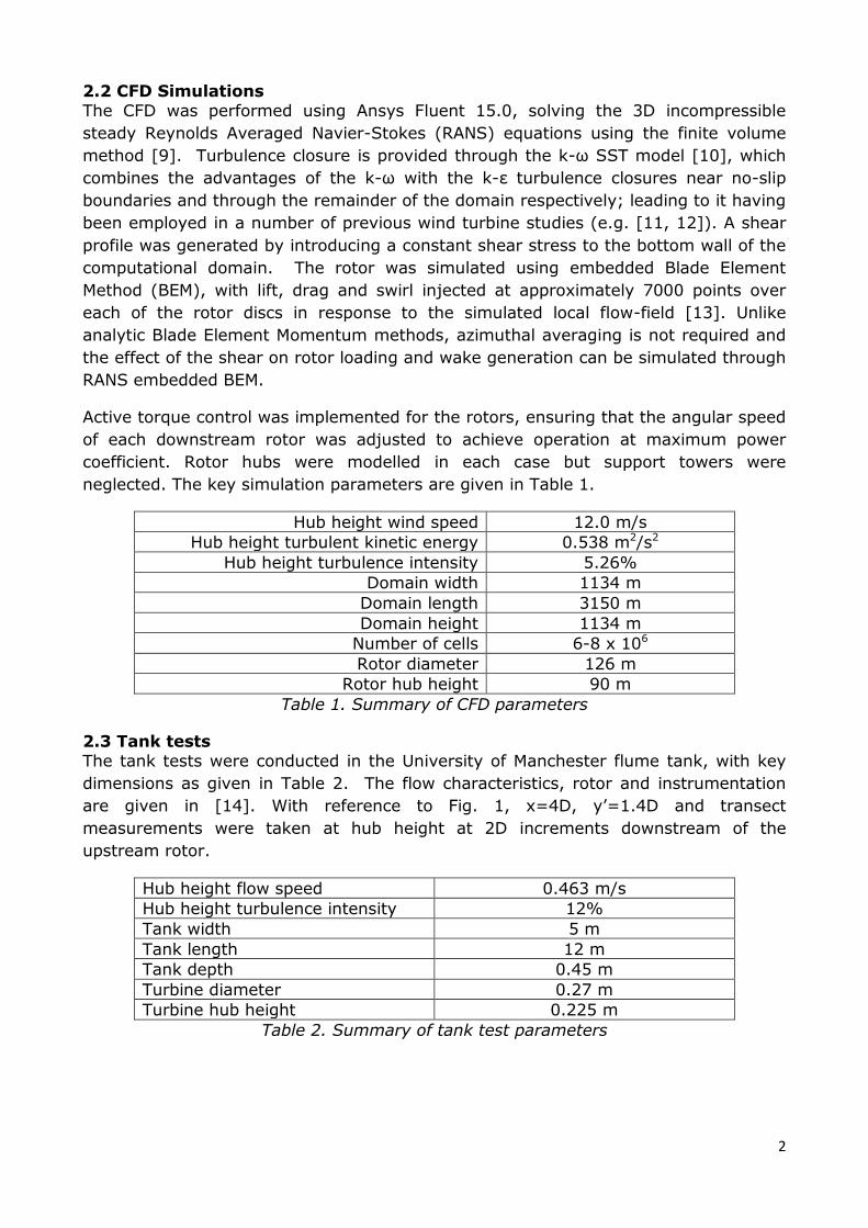
3.2.2 Partly Offset Rotors

Fig. 5 demonstrates that the unphysical largest-deficit approach does not perform well

when the swept area of the downstream rotor is only partly exposed to the wake of

the upstream turbine. Indeed, the simulated effect of the two rotors is a much

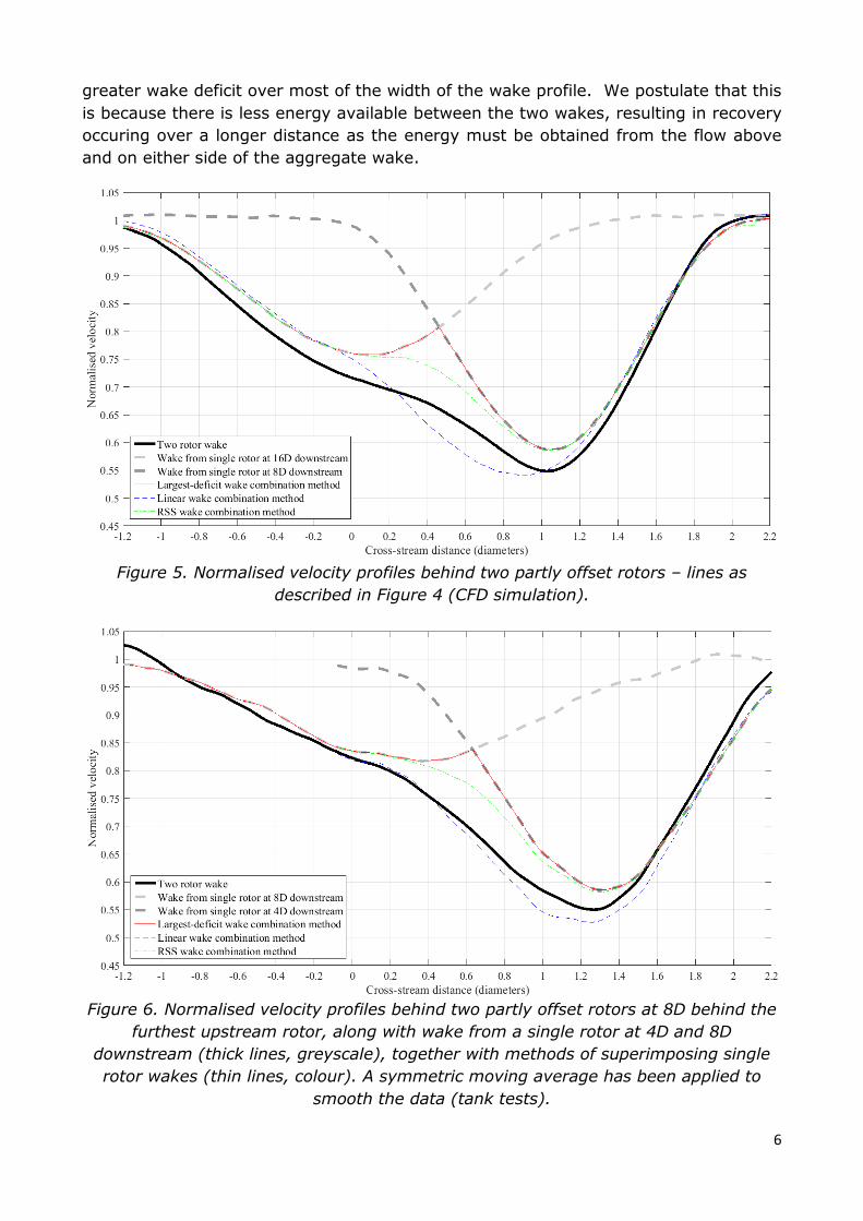
6

greater wake deficit over most of the width of the wake profile. We postulate that this

is because there is less energy available between the two wakes, resulting in recovery

occuring over a longer distance as the energy must be obtained from the flow above

and on either side of the aggregate wake.

Figure 5. Normalised velocity profiles behind two partly offset rotors – lines as

described in Figure 4 (CFD simulation).

Figure 6. Normalised velocity profiles behind two partly offset rotors at 8D behind the

furthest upstream rotor, along with wake from a single rotor at 4D and 8D

downstream (thick lines, greyscale), together with methods of superimposing single

rotor wakes (thin lines, colour). A symmetric moving average has been applied to

smooth the data (tank tests).

7

The effect is corroborated by the velocity measurements from the tank tests, as

shown in Fig. 6 for the same configuration (except with a streamwise turbine

separation of 4D rather than 8D, used due to the more rapid wake expansion at lower

Reynolds numbers in the tank tests).

This situation occurs rather commonly in practice, so correction in analytic models

should be considered to ensure better prediction of average energy yield over the life

of a wind farm. If the direction sector in energy yield validation studies is chosen to

be sufficiently wide (depending on the turbine layout) to average over both partly and

fully in-line cases, this may result in such models providing improved long-term

performance and behaving in a consistent manner when turbine positions are

gradually altered for layout optimisation.

3.2.3 Fully Offset Rotors

The fully offset case demonstrates the most interesting physics. Fig. 7 shows that the

upstream rotor’s wake has been offset by approximately D/8, due to the pressure field

created by the downstream rotor.

Compared with the partly offset or fully in-line cases, the wake due to two fully offset

rotors could therefore not be expressed as a simple combination of single rotor wakes.

This effect is further shown in Figs. 8 and 9.

Figure 7. Normalised velocity profiles at 16D behind two fully offset rotors – lines as

described in Figure 4 (CFD simulation).

8

Figure 8. Normalised velocity map at hub height for two fully offset rotors, flow

incident from the left (CFD simulation)

Figure 9. Normalised velocity cross-section at 12D downstream of the first of two fully

offset turbines (coloured contours). The rotor areas are marked as a black dashed

outlines. The solid black contours indicate the locations of same velocity contours in

the single turbine case, demonstrating how the upstream turbine’s wake has been

shifted and squeezed in the cross-stream direction (CFD simulation).

4 Conclusions

Investigations using CFD simulations of configurations of one and two full-scale wind

turbine rotors have shown that the wake combination methods currently used in

commercially-available analytic energy yield calculation software do not represent

important aspects of the flow physics.

Wake validation studies concentrating on narrow directional sectors with wind flowing

along the axis of a row of turbines have been used to justify largest-deficit wake

9

combination approach in analytical wake models. However, this study has shown

that, when the swept area of the downstream turbine is not fully enclosed in the wake

of the upstream turbine, a much deeper wake deficit is produced than calculated for

the same turbine in isolation, entailing significant error in velocity (and particularly for

power) for the largest-deficit combination approach.

When turbines are located just outside the wake of upstream turbines, this study has

demonstrated emergent flow physics: the pressure field generated by the downstream

rotor shifts the location of the upstream wake laterally and compresses it.

These effects indicate that analytic wind farm models should consider implementing

more than simplistic combination of pre-solved single turbine wakes, for instance by

solving the flow equations of the Eddy Viscosity model developed by Ainslie, but with

explicit consideration of the presence of upstream and nearby turbines.

Space prevents the publication here of several further data sets that have been

collected and analysed. These will be presented in future:

- Further analysis on the best choice of “equivalent” wind speed to predict energy

yield.

- Three-turbine simulations, extending and reinforcing the conclusions here.

- Simulations with pitch control, investigating the change in wake behaviour at

lower rotor thrust.

- Turbulence intensity, particularly whether the normalisation by local flow speed

obscures the evaluation of the turbulent kinetic energy added by rotors.

- Quantification of the impact of the single turbine superposition assumption on

real wind farm energy production estimates.

5 Learning Objectives The objectives of this study were as follows:

To investigate how wakes combine when overlapping (e.g. when the inflow to

the wake-generating turbines is undisturbed) and when interacting (e.g. when

the inflow to at least one of the turbines is partly or wholly in the wake of

another).

To determine whether simple linear wake combination methods as presently

used in commercial analytical software can correctly represent turbine

interactions.

To identify any emergent effects from multiple turbine interactions which have

so far not been widely discussed in the literature.

To identify whether analytical models could be modified to represent large wind

farm arrays more accurately.

To provide phenomenological input to new validation studies of analytical

models against wind farm data – particularly in the selection of test cases for

validation.

10

References

[1] AWS Truepower, “OpenWind Theoretical Basis and Validation,” AWS Truepower, 2010.

[2] DNV GL, “WindFarmer Theory Manual,” DNV GL, 2011.

[3] EMD International, “WindPRO Introduction to Wind Turbine Wake Modelling and Wake Generated

Turbulence,” EMD International, 2011.

[4] S. Ott, J. Berg and M. Nielsen, “Linearised CFD Models for Wakes,” DTU, 2011.

[5] N. O. Jensen, “A Note on Wind Generator Interaction,” Risø-M-2411, 1983.

[6] J. F. Ainslie, “Calculating the Flowfield in the Wake of Wind Turbines,” Journal of Wind Engineering and

Industrial Applications, no. 27, pp. 213-224, 1988.

[7] E. Machefaux, G. C. Larsen and J. P. Murcia Leon, “Engineering models for merging wakes in wind farm

optimization applications,” Journal of Physics: Conference Series, vol. 625, 2015.

[8] J. Jonkman, S. Butterfield, W. Musial and G. Scott, “Definition of a 5-MW Reference Wind Turbine for

Offshore System Development,” NREL/TP-500-38060, 2009.

[9] ANSYS Inc, “ANSYS Fluent 15.0 Theory Guide,” ANSYS Inc, Canonsburg, PA, 2013.

[10] F. R. Menter, “Two-equation eddy-viscosity turbulence models for engineering applications,” AIAA

Journal, vol. 32, no. 8, pp. 1598-1605, 1994.

[11] N. M. Sørensen, J. A. Michelsen and S. Schreck, “Navier-Stokes predictions of the NREL phase VI rotor

in the NASA Ames 80-by-120 wind tunnel,” in 2002 ASME wind energy symposium, Reston, VA,

American Institute of Aeronautics & Astronautics, 2002.

[12] R. Mahu and F. Popescu, “NREL Phase VI rotor modeling and simulation using ANSYS Fluent 12.1,”

Mathematical Modeling in Civil Engineering, no. 1/2, pp. 185-194, 2011.

[13] B. Sanderse, S. P. van der Pijl and B. Koren, “Review of computational fluid dynamics for wind turbine

wake aerodynamics,” Wind Energy, vol. 14, no. 7, pp. 799-819, 2011.

[14] T. Stallard, T. Feng and P. K. Stansby, “Experimental study of the mean wake of a tidal stream rotor in a

shallow turbulent flow,” Journal of Fluids and Structures, vol. 54, pp. 235-246, 2015.

[15] R. Wagner, B. Cañadillas, A. Clifton and J. W. Wagenaar, “Rotor equivalent wind speed for power curve

measurement – comparative exercise for IEA Wind Annex 32,” Journal of Physics: Conference Series,

vol. 524, 2014.

[16] L. J. Vermeer, J. N. Sørensen and A. Crespo, “Wind turbine wake aerodynamics,” Progress in Aerospace

Sciences, vol. 39, pp. 467-510, 2003.

[17] N. G. Nygaard, “Wakes in very large wind farms and the effect of neighbouring wind farms,” Journal of

11

Physics: Conference Series, vol. 524, 2014.

[18] F. Porté-Agel, Y.-T. Wu and C.-H. Chen, “A Numerical Study of the Effects of Wind Direction on Turbine

Wakes and Power Losses in a Large Wind Farm,” Energies, vol. 6, pp. 5297-5313, 2013.

[19] A. Westerhellweg, B. Cañadillas, F. Kinder and T. Neumann, “Wake measurements at alpha ventus -

dependency on stability and turbulence intensity,” 2012.

[20] M. Gaumond, P. E. Réthoré, A. Bechmann, S. Ott, G. C. Larsen, A. Peña and K. S. Hansen,

“Benchmarking of wind turbine wake models in large offshore wind farms,” in Torque 2012, 2012.

[21] J. N. Sørensen, R. Mikkelsen, S. Sarmast, S. Ivanell and D. Henningson, “Determination of Wind Turbine

Near-Wake Length Based on Stability Analysis,” Journal of Physics: Conference Series, vol. 524, 2014.