limits 2. we noticed in section 2.3 that the limit of a function as x approaches a can often be...

LIMITSLIMITS

2

We noticed in Section 2.3 that the limit

of a function as x approaches a can often

be found simply by calculating the value

of the function at a. Functions with this property are called

‘continuous at a.’

LIMITS

2.5Continuity

LIMITS

In this section, we will:

See that the mathematical definition of continuity

corresponds closely with the meaning of the word

continuity in everyday language.

A function f is continuous at a number a if:

lim ( ) ( )x a

f x f a

CONTINUITY 1. Definition

Notice that Definition 1

implicitly requires three things

if f is continuous at a: f(a) is defined—that is, a is in the domain of f exists. .

lim ( )x a

f x

lim ( ) ( )x a

f x f a

CONTINUITY

The definition states that f is

continuous at a if f(x) approaches f(a)

as x approaches a. Thus, a continuous function f

has the property that a small change in x produces only a small change in f(x).

In fact, the change in f(x) can be kept as small as we please by keeping the change in x sufficiently small.

CONTINUITY

If f is defined near a—that is, f is defined on

an open interval containing a, except perhaps

at a—we say that f is discontinuous at a

(or f has a discontinuity at a) if f is not

continuous at a.

CONTINUITY

Physical phenomena are

usually continuous. For instance, the displacement or velocity

of a vehicle varies continuously with time, as does a person’s height.

CONTINUITY

However, discontinuities

do occur in such situations as

electric currents. See Example 6 in Section 2.2, where the Heaviside

function is discontinuous at 0 because does not exist.

0lim ( )tH t

CONTINUITY

Geometrically, you can think of a function

that is continuous at every number in an

interval as a function whose graph has no

break in it. The graph can be drawn without removing

your pen from the paper.

CONTINUITY

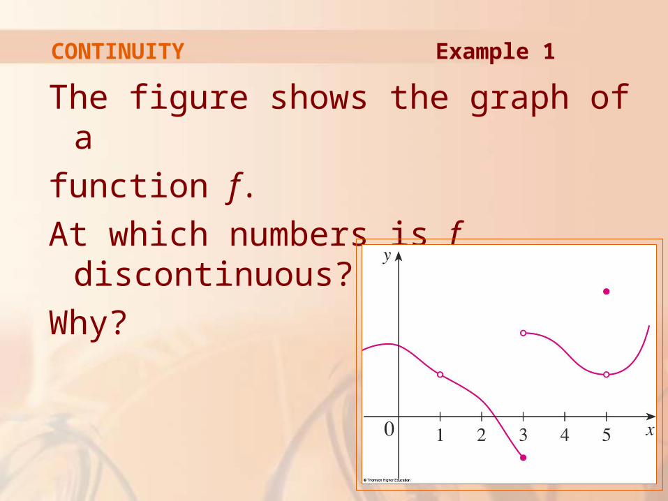
The figure shows the graph of a

function f.

At which numbers is f discontinuous?

Why?

CONTINUITY Example 1

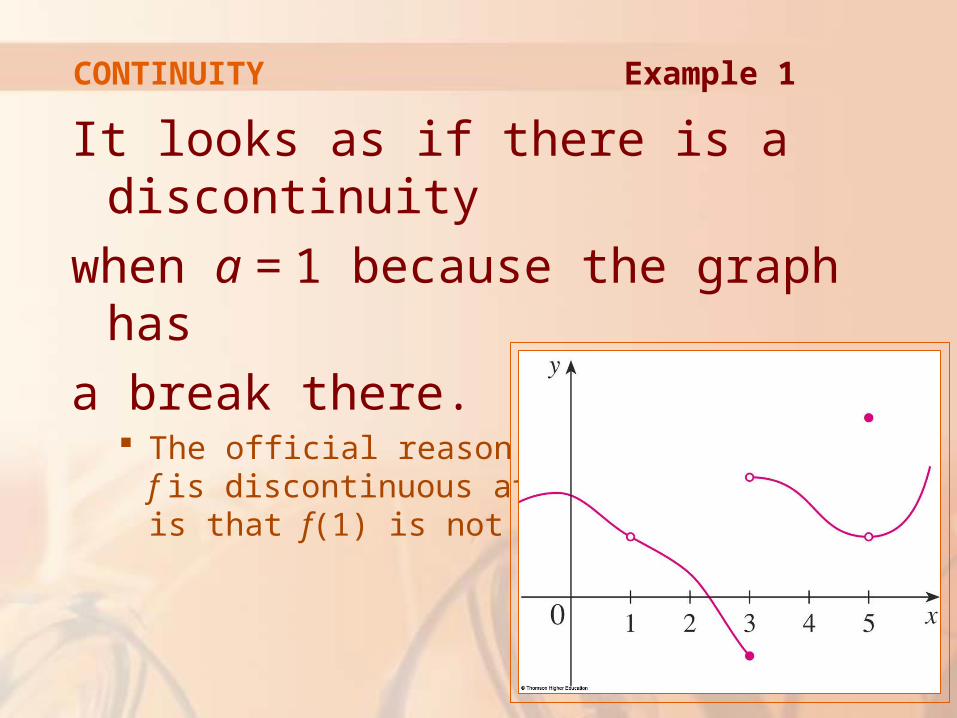
It looks as if there is a discontinuity

when a = 1 because the graph has

a break there. The official reason that

f is discontinuous at 1 is that f(1) is not defined.


The graph also has a break when a = 3.

However, the reason for the discontinuity

is different. Here, f(3) is defined,

but does not exist (because the left and right limits are different).

So, f is discontinuous at 3.

3lim ( )xf x


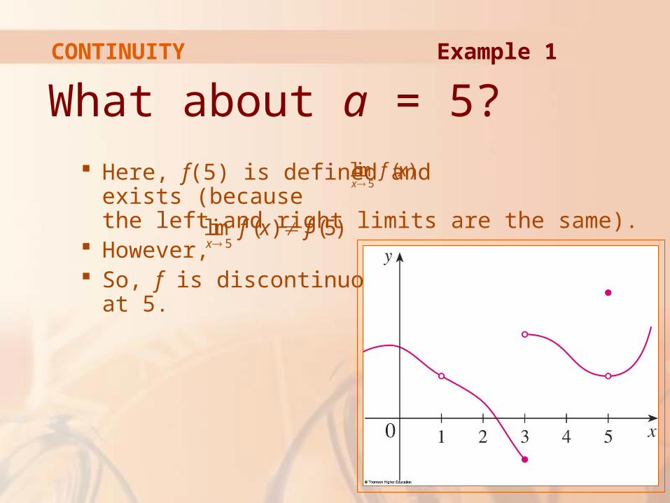
What about a = 5? Here, f(5) is defined and exists (because

the left and right limits are the same). However, So, f is discontinuous

at 5.

5lim ( )xf x

5lim ( ) (5)xf x f


Now, let’s see how to detect

discontinuities when a function

is defined by a formula.

CONTINUITY

Where are each of the following functions

discontinuous?

a.

b.

c.

d. f (x) x


2 2( )

2

x xf x

x

2

10

( )1 0

if xf x x

if x

2 22

( ) 21 2

x xif x

f x xif x

Notice that f(2) is not defined.

So, f is discontinuous at 2. Later, we’ll see why f is continuous

at all other numbers.

CONTINUITY Example 2 a

Here, f(0) = 1 is defined.

However, does not exist. See Example 8 in Section 2.2.

So, f is discontinuous at 0.

20 0

1lim ( ) limx xf x

x

CONTINUITY Example 2 b

Here, f(2) = 1 is defined and

exists.

However,

So, f is not continuous at 2.

2

2 2

2

2

2lim ( ) lim

2( 2)( 1)

lim2

lim( 1) 3

x x

x

x

x xf x

xx x

xx

2lim ( ) (2)x

f x f

CONTINUITY Example 2 c

The greatest integer function

has discontinuities at all the integers.

This is because does not exist

if n is an integer. See Example 10 in Section 2.3.

f (x) x

limx n

x

CONTINUITY Example 2 d

The figure shows the graphs of the

functions in Example 2. In each case, the graph can’t be drawn without lifting

the pen from the paper—because a hole or break or jump occurs in the graph.

CONTINUITY

The kind of discontinuity illustrated in

parts (a) and (c) is called removable. We could remove the discontinuity by redefining f

at just the single number 2. The function is continuous.

CONTINUITY

( ) 1g x x

The discontinuity in part (b) is called

an infinite discontinuity.

CONTINUITY

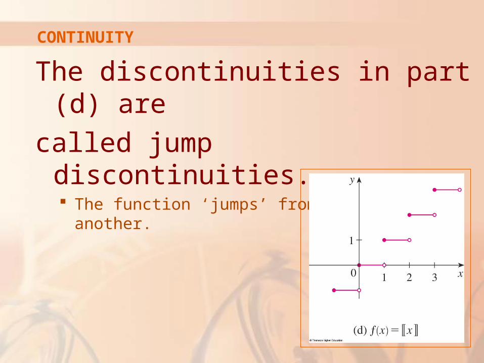
The discontinuities in part (d) are

called jump discontinuities. The function ‘jumps’ from one value to another.

CONTINUITY

A function f is continuous from the right

at a number a if

and f is continuous from the left at a if

lim ( ) ( )x a

f x f a

lim ( ) ( )x a

f x f a


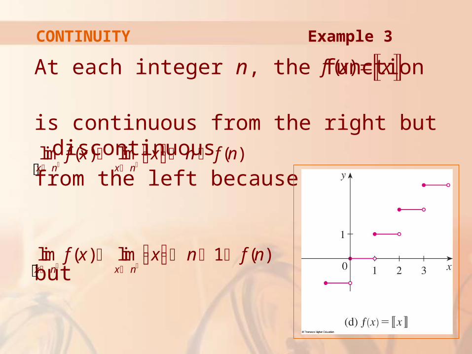
At each integer n, the function

is continuous from the right but discontinuous

from the left because

but

( )f x x

limx n

f (x) limx n

x n f (n)

limx n

f (x) limx n

x n 1 f (n)


A function f is continuous on an

interval if it is continuous at every

number in the interval. If f is defined only on one side of an endpoint of the

interval, we understand ‘continuous at the endpoint’ to mean ‘continuous from the right’ or ‘continuous from the left.’


Show that the function

is continuous on

the interval [-1, 1].

2( ) 1 1f x x


If -1 < a < 1, then using the Limit Laws,

we have:

2

2

2

2

lim ( ) lim(1 1 )

1 lim 1 (by Laws 2 and 7)

1 lim(1 ) (by Law 11)

1 1 (by Laws 2, 7, and 9)

( )

x a x a

x a

x a

f x x

x

x

a

f a


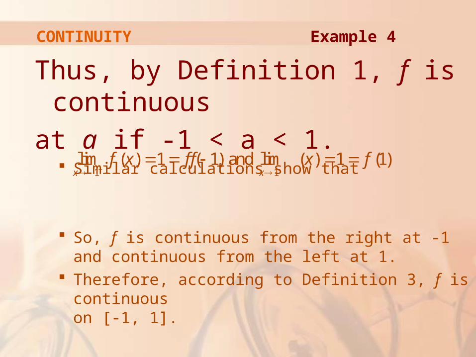
Thus, by Definition 1, f is continuous

at a if -1 < a < 1. Similar calculations show that

So, f is continuous from the right at -1 and continuous from the left at 1.

Therefore, according to Definition 3, f is continuous on [-1, 1].

1 1lim ( ) 1 ( 1) and lim ( ) 1 (1)x x

f x f f x f


The graph of f is sketched in

the figure. It is the lower half of the circle

2 2( 1) 1x y


Instead of always using Definitions 1,

2, and 3 to verify the continuity of

a function, as we did in Example 4,

it is often convenient to use the next

theorem. It shows how to build up complicated continuous

functions from simple ones.

CONTINUITY

If f and g are continuous at a, and c is

a constant, then the following functions

are also continuous at a:

1. f + g

2. f - g

3. cf

4. fg

5. ( ) 0fif g a

g

CONTINUITY 4. Theorem

Each of the five parts of the theorem

follows from the corresponding Limit Law

in Section 2.3. For instance, we give the proof of part 1.

CONTINUITY

Since f and g are continuous at a, we have:

Therefore,

This shows that f + g is continuous at a.

lim( )( ) lim ( ) ( )

lim ( ) lim ( ) (byLaw1)

( ) ( )

( )( )

x a x a

x a x a

f g x f x g x

f x g x

f a g a

f g a

lim ( ) ( ) and lim ( ) ( )x a x a

f x f a g x g a

ProofCONTINUITY

It follows from Theorem 4 and

Definition 3 that, if f and g are continuous

on an interval, then so are the functions

f + g, f - g, cf, fg, and (if g is never 0) f/g.

CONTINUITY

The following theorem was

stated in Section 2.3 as

the Direct Substitution Property.

CONTINUITY

a. Any polynomial is continuous everywhere—that is, it is continuous on

b. Any rational function is continuous wherever it is defined—that is, it is continuous on its domain.

( , )= - ¥ ¥¡


As an illustration of Theorem 5,

observe that the volume of a sphere

varies continuously with its radius. This is because the formula

shows that V is a polynomial function of r.

34( )

3V r r

CONTINUITY

Similarly, if a ball is thrown vertically into

the air with a velocity of 50 ft/s, then the

height of the ball in feet t seconds later is

given by the formula h = 50t - 16t2. Again, this is a polynomial function. So, the height is a continuous function

of the elapsed time.

CONTINUITY

Knowledge of which functions are

continuous enables us to evaluate some

limits very quickly—as the following

example shows. Compare it with Example 2(b) in Section 2.3.

CONTINUITY

Find

The function is rational.

So, by Theorem 5, it is continuous on its domain, which is:

Therefore,

3 2

2

2 1lim

5 3x

x x

x

3 22 1( )

5 3

x xf x

x

5|

3x x


3 2 3 2

2 2

2 1 ( 2) 2( 2) 1 1lim lim ( ) ( 2)

5 3 5 3( 2) 11x x

x xf x f

x

It turns out that most of the familiar

functions are continuous at every

number in their domains. For instance, Limit Law 10 is exactly the statement

that root functions are continuous.

CONTINUITY

From the appearance of the graphs

of the sine and cosine functions, we

would certainly guess that they are

continuous.

CONTINUITY

We know from the definitions of and that the coordinates of the point P in the figure are . As , we see that P approaches the point (1, 0) and

so and . Thus,

sincos

(cos , sin ) 0 cos 1 sin 0

0 0limcos 1 limsin 0


Since and , the

equations in Definition 6 assert that

the cosine and sine functions are

continuous at 0. The addition formulas for cosine and sine can then

be used to deduce that these functions are continuous everywhere.

cos0 1 sin 0 0CONTINUITY

It follows from part 5 of Theorem 4

that is continuous

except where cos x = 0.

CONTINUITY

sintan

cos

xx

x

This happens when x is an odd integer

multiple of .

So, y = tan x has infinite discontinuities

when

and so on.

2

3 52, 2, 2,x

CONTINUITY

The following types of functions

are continuous at every number

in their domains: Polynomials Rational functions Root functions Trigonometric functions


Evaluate

Theorem 7 gives us that y = sin x is continuous. The function in the denominator, y = 2 + cos x,

is the sum of two continuous functions and is therefore continuous.

Notice that this function is never 0 because for all x and so 2 + cos x > 0 everywhere.

sinlim2 cosx

x

x

cos 1


Thus, the ratio is continuous everywhere.

Hence, by the definition of a continuous function,

sin( )

2 cos

xf x

x

sinlim lim ( )2

( )

sin

20

02 1

x x

xf x

cosxf

cos


Another way of combining

continuous functions f and g to get

a new continuous function is to form

the composite function This fact is a consequence

of the following theorem.

f g

CONTINUITY

If f is continuous at b and , then

In other words,

Intuitively, Theorem 8 is reasonable. If x is close to a, then g(x) is close to b; and, since f

is continuous at b, if g(x) is close to b, then f(g(x)) is close to f(b).

lim ( )x ag x b

lim ( ( )) ( )x a

f g x f b

lim ( ( )) lim ( )x a x a

f g x f g x


Let’s now apply Theorem 8 in the special

case where , with n being

a positive integer. Then, and

If we put these expressions into Theorem 8, we get:

So, Limit Law 11 has now been proved. (We assume that the roots exist.)

( ) nf x x

( ( )) ( )nf g x g x (lim ( )) lim ( )nx a x a

f g x g x

CONTINUITY

lim ( ) lim ( )n nx a x a

g x g x

If g is continuous at a and f is continuous

at g(a), then the composite function

given by is continuous

at a. This theorem is often expressed informally by saying

“a continuous function of a continuous function is a continuous function.”

f g ( ) ( ( ))f g x f g x


Where are these functions continuous?

a.

b.

2( ) sin( )h x x


2

1( )

7 4

F x

x

We have h(x) = f(g(x)), where

and

Now, g is continuous on since it is a polynomial, and f is also continuous everywhere.

Thus, is continuous on by Theorem 9.

2( )g x x ( ) sinf x x

h f g

CONTINUITY Example 8 a

Notice that F can be broken up as the

composition of four continuous functions

where:

Example 8 bCONTINUITY

orF f g h k F x f g h k x

21, 4 , , 7f x g x x h x x k x x

x

We know that each of these functions is

continuous on its domain (by Theorems

5 and 7).

So, by Theorem 9, F is continuous on its domain,which is:

CONTINUITY Example 8 b

2| 7 4 | 3

, 3 3, 3 3,

x x x x

An important property of

continuous functions is expressed

by the following theorem. Its proof is found in more advanced books on

calculus.

CONTINUITY

Suppose that f is continuous on the closed

interval [a, b] and let N be any number

between f(a) and f(b), where .

Then, there exists a number c in (a, b)

such that f(c) = N.

( ) ( )f a f b

INTERMEDIATE VALUE THEOREM 10. Theorem

The theorem states that a continuous

function takes on every intermediate

value between the function values f(a)

and f(b).

INTERMEDIATE VALUE THEOREM

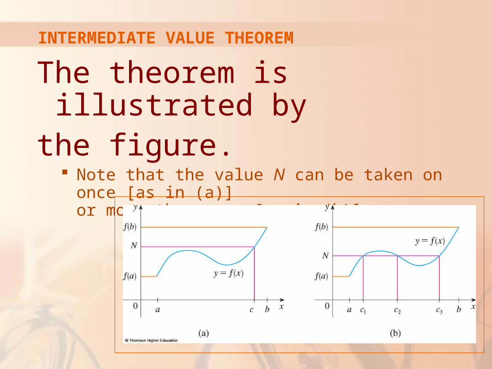
The theorem is illustrated by the figure. Note that the value N can be taken on once [as in (a)]

or more than once [as in (b)].


If we think of a continuous function as a function whose graph has no hole or break, then it is easy to believe that the theorem is true.


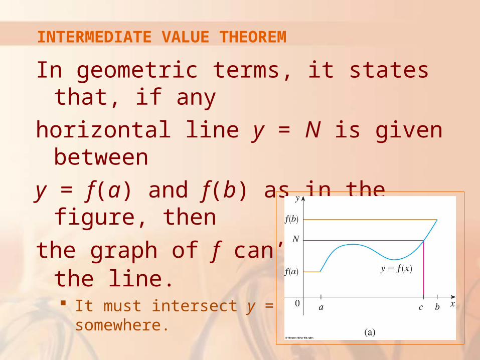
In geometric terms, it states that, if any

horizontal line y = N is given between

y = f(a) and f(b) as in the figure, then

the graph of f can’t jump over the line. It must intersect y = N

somewhere.


It is important that the function in

the theorem be continuous. The theorem is not true in general for

discontinuous functions.


One use of the theorem is in

locating roots of equations—as in

the following example.


Show that there is a root of the equation

between 1 and 2.

Let . We are looking for a solution of the given equation—

that is, a number c between 1 and 2 such that f(c) = 0. Therefore, we take a = 1, b = 2, and N = 0 in

the theorem. We have

and

3 24 6 3 2 0x x x 3 2( ) 4 6 3 2f x x x x

INTERMEDIATE VALUE THEOREM Example 9

(1) 4 6 3 2 1 0f (2) 32 24 6 2 12 0f

Thus, f(1) < 0 < f(2)—that is, N = 0 is a number between f(1) and f(2).

Now, f is continuous since it is a polynomial. So, the theorem states that there is a number c

between 1 and 2 such that f(c) = 0. In other words, the equation

has at least one root in the interval (1, 2).

3 24 6 3 2 0x x x


In fact, we can locate a root more precisely by using the theorem again.

Since a root must lie between 1.2 and 1.3.

A calculator gives, by trial and error,

So, a root lies in the interval (1.22, 1.23).

(1.2) 0.128 0 and (1.3) 0.548 0f f

(1.22) 0.007008 0 and (1.23) 0.056068 0f f


limits 2. we noticed in section 2.3 that the limit of a function as x approaches a can often be...

Documents

f discontinuous

continuous function

continuityif f

domain of f

heaviside function

small change

cthe greatest integer

fx approaches fa