limits and tradeoffs in the control of ...thesis.library.caltech.edu/7825/196/thesisfinal.pdflimits...
TRANSCRIPT

LIMITS AND TRADEOFFS IN THE
CONTROL OF AUTOCATALYTIC
SYSTEMS
Thesis by
Fiona Chandra
In Partial Fulfillment of the Requirements for the degree
of
Doctor of Philosophy in Bioengineering
CALIFORNIA INSTITUTE OF TECHNOLOGY
Pasadena, California
2013
(Defended May 29, 2013)

ii
2013
Fiona Chandra
All Rights Reserved

iii ACKNOWLEDGEMENTS
I would like to thank my advisor John Doyle and committee members Richard Murray, Joe
DiStefano, and Erik Winfree. I would also like to thank Professor Hana El-Samad, Jacob Stewart-
Ornstein, Ophelia Venturelli for lending their help, lab space and equipments for my experiments,
Josh Michener, Genti Buzi, Vanessa Jonsson, (and Ophelia again) and all the Indonesian students at
Caltech for all their feedback and friendship over the years. Last but not least, I would like to thank
my parents for their support and for patiently waiting for my graduation.

iv ABSTRACT
Despite the complexity of biological networks, we find that certain common architectures govern
network structures. These architectures impose fundamental constraints on system performance and
create tradeoffs that the system must balance in the face of uncertainty in the environment. This
means that while a system may be optimized for a specific function through evolution, the optimal
achievable state must follow these constraints. One such constraining architecture is autocatalysis,
as seen in many biological networks including glycolysis and ribosomal protein synthesis. Using a
minimal model, we show that ATP autocatalysis in glycolysis imposes stability and performance
constraints and that the experimentally well-studied glycolytic oscillations are in fact a consequence
of a tradeoff between error minimization and stability. We also show that additional complexity in
the network results in increased robustness. Ribosome synthesis is also autocatalytic where
ribosomes must be used to make more ribosomal proteins. When ribosomes have higher protein
content, the autocatalysis is increased. We show that this autocatalysis destabilizes the system,
slows down response, and also constrains the system’s performance. On a larger scale,
transcriptional regulation of whole organisms also follows architectural constraints and this can be
seen in the differences between bacterial and yeast transcription networks. We show that the degree
distributions of bacterial transcription network follow a power law distribution while the yeast
network follows an exponential distribution. We then explored the evolutionary models that have
previously been proposed and show that neither the preferential linking model nor the duplication-
divergence model of network evolution generates the power-law, hierarchical structure found in
bacteria. However, in real biological systems, the generation of new nodes occurs through both
duplication and horizontal gene transfers, and we show that a biologically reasonable combination
of the two mechanisms generates the desired network.

v TABLE OF CONTENTS
Acknowledgements ........................................................................................................ iii
Abstract ........................................................................................................................... iv
Table of Contents ............................................................................................................ v
List of Illustrations and/or Tables .................................................................................. vi
Chapter I: Introduction .................................................................................................... 1
Chapter II: Minimal Model of Glycolytic Oscillations: Limits and Tradeoffs ............. 4
Minimal Model ......................................................................................................... 4
Steady State Limits ................................................................................................... 7
Hard Limits on Robust Efficiency ......................................................................... 11
Complexity and Robustness ................................................................................... 16
Experiments in Single Cells ................................................................................... 21
Chapter III: Single Cell Oscillations and Redox ......................................................... 28
Oscillations in Single Yeast Cells .......................................................................... 28
Analysis of the Kloster Model ............................................................................... 29
Redox Balance in Anaerobic S. cerevisiae ............................................................ 31
Glycolysis Model with Redox and Diffusion ........................................................ 32
The Role of Glycerol Production ........................................................................... 40
Chapter IV: Ribosome Autocatalysis ........................................................................... 43
Minimal Model of Ribosome Synthesis ................................................................ 44
Higher Order Model of Ribosome Synthesis ......................................................... 47
Tradeoffs in Ribosome Synthesis: Maximal Growth and Efficiency ................... 49
Tradeoffs in Ribosome Synthesis: Feedback and Stability ................................... 49
Ribosome Synthesis During Starvation ................................................................. 51
Three-State Model of Ribosome Autocatalysis ..................................................... 53
Mitochondrial Ribosomes ...................................................................................... 63
Ribosome Heterogeneity ........................................................................................ 64
Chapter V: Evolution of Network Architecture ........................................................... 66
Power Law Distributions and Scale Free-ness ...................................................... 66
Transcription Network Architectures in Bacteria vs Yeast ................................... 67
Comparison of Generating Models ........................................................................ 71
A Biologically Relevant Combined Model ........................................................... 73
Prokaryotic vs Eukaryotic Regulation ................................................................... 76
Chapter VI: Conclusions ............................................................................................... 78
Bibliography .................................................................................................................. 83

vi LIST OF ILLUSTRATIONS AND/OR TABLES
Figure Number Page
2.1 Diagram of the two-state glycolysis model ....................................................... 7
2.2 The equilibrium point(s) of the system ............................................................. 9
2.3 Tradeoffs between waste, fragility, and complexity ....................................... 10
2.4 Effects of higher autocatalytic stoichiometry q ....................................... 15
2.5 Log Sensitivity and step response of glycolysis without PK feedback .......... 17
2.6 Log Sensitivity and step response a) with PK feedback b) with varying k .... 19
2.7 Histogram of glycolytic enzyme in cells grown in glucose vs ethanol ......... 22
2.8 NADH autofluorescence in single cells grown in ethanol ............................. 25
2.9 NADH autofluorescence in single cells grown in glucose ............................. 25
2.10 Simulation of two state model recapitulating cell extract studies .................. 27
3.1 Linear stability regions of Kloster et al’s model ............................................. 31
3.2 Glycolysis models incorporating redox and diffusion .................................... 35
3.3 Stability regions of 7-dimensional glycolysis model ..................................... 36
3.4 Stability regions of the 4-state glycolysis model ............................................ 37
3.5 Extracellular acetaldehyde concentration ...................................................... 38
3.6 Stability analysis for varying NAD+ autocatalytic stoichiometry ................. 39
3.7 Stability regions for varying number of NAD+ molecules and produced ..... 39
3.8 Stability changes with the interaction of the two autocatalytic loops ............ 40
3.9 Higher glycerol production rate is stabilizing ................................................. 41
4.1 Growth rate for varying ribosome production ratio ........................................ 46
4.2 Diagram of the 6-state ribosome synthesis model .......................................... 47
4.3 Optimal ratio for growth and proportion of ribosomes in the cell ................. 48
4.4 Stability regions mRNA production rates are varied ...................................... 50
4.5 Simulation of the 6-state ribosome model ..................................................... 51
4.6 Sensitivity of steady state levels to various parameter perturbations ............. 52
4.7 Optimal ratio for highest protein level in starvation condition....................... 53
4.8 Simulation of the 6-state ribosome model to sudden nutrient availability ..... 54
4.9 Optimal riboprotein transcription ratio increases with nutrient level ............ 55
4.10 Stability region of 3-state ribosome model with varying autocatalysis ......... 56

vii 4.11 Cost of cell growth ........................................................................................... 57
4.12 Higher autocatalysis slows down response time ............................................. 57
4.13 Minimum stable ratio as rRNA level increases .......................................... …58
4.14 Optimal and minimum stable ratio as feedback strength increases ............ …59
4.15 Optimal and minimum stable ratio as autocatalysis increases ................... …59
4.16 Poles of 3-state ribosome model with varying rm and autocatalysis .......... …61
4.17 Zeros of 3-state ribosome model with feedback from ribosomal protein to translation…61
4.18 Zeros of 3-state ribosome model with feedback from ribosomes to rRNA…62
4.19 At lower rRNA level, the system requires lower autocatalysis to maintain stability…65
5.1 Rank-degree plot of transcriptional regulatory networks ............................... 68
5.2 In-degree plot of transcriptional regulatory networks .................................... 68
5.3 Rank-degree plot of the operon-operon regulatory network in E. coli .......... 70
5.4 The clustering coefficients of all three organisms .......................................... 70
5.5 Clustering coefficients of the network generated by Yule process ................ 72
5.6 Degree distributions of networks generated by Yule process and duplication divergence
...................................................................................................................... …74
5.7 A small power-law network is expanded via the duplication divergence mechanism …75
5.8 Distribution of network simulated with combined network model mimic E. coli network
...................................................................................................................... …76
5.9 Clustering coefficients of the network generated by combined model .......... 76
Table Number Page
1. Parameters and definition of terms of the glycolysis model............................. 5
2. Tradeoffs in glycolysis with respect to various parameters............................ 21
3. Fluorescence statistics of GFP-tagged glycolytic enzymes ............................ 22
4. Parameter definitions of the 6-state ribosome model .................................... 48
5. Statistics of the three transcription networks .................................................. 69
Equation Section (Next)

1
Equation Section (Next) Chapter 1
INTRODUCTION
Minimizing waste, resource use, and fragility to perturbations in system components, operation, and
environment (1) is crucial to sustainability of systems ranging from cells to engineering
infrastructure. Much of the studies of the evolutionary basis of biological networks have been based
on the idea that the networks optimize growth rate, but both engineering and biology are
constrained by tradeoffs between efficiency and robustness which are rarely formalized in biology.
Tools that are commonly used in optimization as well as in systems and control theory can provide
a good foundation in understanding these tradeoffs in biological networks.
Certain network architectures have aggravated constraints and tradeoffs (2). One such architecture
is autocatalysis, where a species is consumed in catalyzing its own production. This type of
structure can grow uncontrollably without feedback regulation, yet we find autocatalysis in many
crucial functions of the cell, including metabolism (glycolysis) and protein synthesis. Some
autocatalysis is unavoidable due to the reaction energetics requirements as in the case of glycolysis.
Glycolysis is a central energy producer in a living cell, consuming glucose to generate Adenosine
Triphosphate (ATP) which is used throughout the cell. The first steps of the reaction require ATP,
making it autocatalytic. The energy input from ATP hydrolysis is necessary to power
thermodynamically unfavorable reactions.
Using the well-studied problem of glycolytic oscillation as a case study, we integrated concepts
from biochemistry and control theory to explore the hard limits of robust efficiency. We chose

2 glycolysis as a first case study, as it not only has interesting dynamics (e.g. oscillations) but has a
rich literature experimentally and theoretically (3). Despite extensive experimental and modeling
studies since 1965 (4), whether the oscillations are beneficial or simply an evolutionary accident
remained unsolved. Using control theoretic analysis on a simple model, we suggest a third
alternative: Oscillations are the inevitable consequence of tradeoffs between metabolic overhead
and robustness to disturbances, as well as the interplay between feedback control and necessary
autocatalysis of network products (5, 6). Our model is now also the simplest (with only two states)
example of a system with a right-half plane zero and can be used as a tool for teaching some
fundamental concepts of control theory.
Glycolysis is one of the most common pathways in biology, but there is another universal system
that is autocatalytic: protein synthesis. Proteins are synthesized by ribosomes, which are part RNA
(called ribosomal RNA, rRNA) and part protein (called ribosomal proteins or riboproteins). The
protein components of the ribosomes must also be synthesized by ribosomes themselves, resulting
in not only an autocatalytic loop but a resource competition between riboproteins and all other non-
ribosomal proteins. The cell must decide how much of the available ribosomes should be used to
make more ribosomal proteins instead of growth proteins. How the cell balances this resource
during different growth conditions such as maximal growth and starvation, and how it manages the
consequences of the autocatalytic loop, is of great interest. There has been a recent surge of interest
in the problem of resource allocation/competition, particularly with ribosomes, since the growth of
the field of synthetic biology (7, 8), but the autocatalytic nature of the process has not been
discussed. Here we explore different models capturing resource competition and autocatalysis in
terms of the protein content of ribosomes.

3 At a larger scale biology is still governed by various architectures. Regulation of gene expression
is layered, with only specific regulatory proteins and RNA able to bind to DNA and control gene
expression. The success of complex communication networks has largely been the result of
adopting such layered architecture (9). However, combinatorial regulation using transcription
factors pose a cost in the size of the genome. There is evidence that, in prokaryotes, the number of
transcription factors scales quadratically to the number of total genes (10), yet the genome size of
prokaryotes seems to be constrained at around 9000 genes by metabolism and cell size (11). The
quadratic scaling is certainly not seen when we go from prokaryotes to higher eukaryotes. In
bacteria the regulation is largely achieved by regulatory proteins (called transcription factors) and a
class of small RNAs, while eukaryotes have many more noncoding regulatory RNAs (such as micro
RNAs, small nuclear RNAs, small interfering RNAs) and can also regulate expression by
alternative splicing. The transcription regulation network is very complex even in small, single cell
organisms such as bacteria, but graph theoretic analysis can be used to study some general
properties. The degree distributions of Bacillus subtilis, Escherichia coli, and Saccharomyces
cerevisiae transcription networks reveal that there are, in fact, fundamental differences between
prokaryotic and eukaryotic regulations.

4 C h a p t e r 2
MINIMAL MODEL OF GLYCOLYTIC OSCILLATIONS: LIMITS AND TRADEOFFS
Glycolytic oscillation, in which the concentrations of metabolites fluctuate, has been a classic case
for both theoretical and experimental study in control and dynamical systems since the 1960s (12).
Numerous mathematical models have been developed, from minimal models (4, 13) to those with
extensive mechanistic detail (14). Besides being the most studied control system and the most
common, glycolysis is also conserved from bacteria to human, and presumably has been under
intense evolutionary pressure for robust efficiency. Thus new insights are less likely to be
confounded by either gaps in the literature or evolutionary accidents compared with less well
studied biological circuitry. Nevertheless, the function of the oscillations, if any, remains a mystery
and one we aim to resolve.
The first step is development of the simplest possible model of glycolysis that illustrates the
tradeoffs caused by autocatalysis. Biologically motivated minimal models of glycolytic oscillations
exist, but analysis of robustness and efficiency tradeoffs has not received much attention. Such
analysis can provide a much deeper understanding of the underlying basis of glycolytic oscillations,
as well as illustrate universal laws that are broadly applicable.
Minimal Model
Early experiments in S. cerevisiae observed two synchronized pools of oscillating metabolites (12),
suggesting that a two-state model incorporating Phosphofructokinase (PFK) might capture some
aspects of system dynamics and indeed, such simplified models (4, 13) qualitatively reproduce the
experimental behavior. We propose a minimal system with three reactions (shown in Fig 2.1A), for
which we can identify specific mechanisms both necessary and sufficient for oscillations.

5
2 2
2 2
2 2
2 21 1 0
1 1 2 2
1 12 2( 1) (1 )( 1) (1 )
1 1
a
h g a
h ga
h g
y kxx
y y y kx
y yy kxq qy q q
y yPFK PK Consumption
(2.1)
Model Parameters Definition of Terms
x lumped variable of intermediate
metabolites
P(s) Open loop response (h=0) in frequency
(s) domain
y output, ATP level
k intermediate reaction rate WS(s) Weighted response to a disturbance .
WS(s)=W(s)S(s) where W(s) is the weight perturbation in ATP consumption
q autocatalytic stoichiometry S(s) Impulse response to a disturbance
a cooperativity of ATP binding to PFK z Zero, the solution to P(z)=0
h feedback strength of ATP on PFK p Pole, the solution to W(p)=P(p)=∞, or
D(p)=0
g feedback strength of ATP on PK
Table 1.
In the first reaction in (2.1), PFK consumes q molecules of y (ATP) with allosteric inhibition by
ATP. We lump the intermediate metabolites into one variable, x. In the second reaction, Pyruvate
Kinase (PK) produces q+1 molecules of y for a net (normalized) production of 1 unit, which is
consumed in a final reaction representing the cell’s use of ATP. In glycolysis, 2 ATP molecules are
consumed upstream and 4 are produced downstream, which normalizes to q=1 (each y molecule
produces 2 downstream) with kinetic exponent a=1. To highlight essential tradeoffs with the
simplest possible analysis, we normalized the concentration such that the unperturbed ( 0 )
steady states are 1y and 1/x k (the system can have one additional steady state which is
unstable when (1, 1/k) is stable). The basal rate of PFK reaction and consumption rate have been
normalized to 1 (the 2 in the numerator and feedback coefficients of the reactions come from these

6 normalizations). Our results hold for more general systems as discussed below and in SI, but the
analysis is less transparent.
Like most research, we focus on allosteric activation of the enzyme PFK by Adenosine
Monophosphate (AMP) as the main control point of glycolysis. We assume total concentration of
adenosine phosphates in the cell [Atot]=[ATP]+[ADP]+[AMP] remains constant and the activating
effects of AMP can be modeled as ATP inhibition. ATP also inhibits PK activity, although this has
been largely ignored in most models (except (15, 16)). We emphasize its importance and model
both inhibitions through exponents h and g.
We use linearization to focus initially on steady state error and instability while highlighting
disturbance and control:
10
( 1) ( 1) 1
Disturbance Control
x xk a gh y
y y qq k qa g q
(2.2)
The first term on the right hand side (RHS) gives the dynamics of the “open loop” plant (P, defined
as (2.2) when there is no control, i.e. h=0; solid and dotted loop in Fig 2.1A or solid box in Fig
2.1B) in response to the second term (disturbance in demand), while the third is the control on PFK
(dashed loop in Fig 2.1A).

7
Figure 2.1. (A) Diagram of two state glycolysis model. ATP along with constant glucose input
produce a pool of intermediate metabolites (phosphorylated six-carbon sugars), which then
produces two ATPs. ATP inhibits both the first (Phosphofructokinase/PFK-like) and second
(Pyruvate Kinase/PK-like) reactions. (B) Control-theoretic diagram of the same system (arrows
represent logical connections, not fluxes.) The system without inhibition/feedback is labeled the
“Plant” (P; solid box, solid and dotted loop in (A)) while the inhibitory mechanism is considered
the “Controller” (here labeled by its inhibitory strength, H; dashed loop in (A) and (B).) The effect
of disturbance in ATP demand is modeled as the system W (see text for definition).
Steady State Limits
The simplest robust performance requirement (motivated by the need to maintain high energy
charge) is that the concentration of y remain nearly constant despite fluctuating demand . In our
model this requires that the steady state error ratio, obtained by solving for y
when
0
0
x
y
1y
h a
(2.3)
be small, or |h-a| large, and /y 0 if and only if h∞. One tradeoff is that large h requires
either high cooperativity or very tight ATP-enzyme binding, and the resulting complex enzymes are

8 more costly for the cell to produce. A more interesting tradeoff arises because (2.2) is stable if and
only if
10
k g qh a
q
(2.4)
The left boundary indicates where the system is unstable (unstable node) while the right boundary
indicates where the system starts to oscillate (limit cycle).
We can plot f(y) vs. y and the equilibrium points are the intersections of f(y) and the consumption
rate of ATP, which in this model is normalized to 1 (Figure 2.2). There is one equilibrium point
when 2a h (Fig 2.2A and B) and two when 2a h (Fig 2.2C and D). We can show using linear
stability analysis that when the (1, 1/k) equilibrium point is either stable or in a limit cycle, the other
equilibrium point is always unstable, with one positive and one negative eigenvalue (a saddle node).
In fact, we can show that the equilibrium point is unstable when the slope of f(y) is positive and thus
the lower equilibrium point is unstable. If we relax the normalization for ATP consumption then the
equilibrium point moves with the consumption. A study by Kloster and Olsen also confirms that the
activity of intracellular ATPase significantly affects oscillations (17).
The left hand side (LHS) of (2.4) bounds the minimum feedback strength h required to stabilize the
system, so autocatalysis requires some minimal enzyme complexity for stability, but this is
compatible with making (2.3) small. (Experimentally observed PFK activity in response to ATP
suggests that indeed h>a. When h<=a, PFK activity would be monotonically increasing with ATP
but when h>a, PFK activity would increase at low ATP then peaks and starts decreasing). The latter
behavior has been observed in PFK of many organisms (18, 19). More significantly, combining
(2.3) and (2.4) constrains the minimum stable steady state error to:

9
1
1
y q
h a k g q
(2.5)
Figure 2.2. The equilibrium point(s) of the system is given by the intersection(s) of the curve f(y)
(blue) with 1 (red). A) a=h=1. B) a =1 < h=2. C) a=1 < h=8. D) a=5 < h=8.
Equation (2.5) and Fig 2.3A (showing the error bound (2.5) versus k) illustrate a simple and elegant
tradeoff between robustness and efficiency (as measured by complexity and metabolic overhead).
Low error requires large h, but to allow this to be stable, k and/or g must also be large enough.
Large k requires either more efficient or higher level of enzymes, and large g requires a more
complex allosterically controlled PK enzyme; both would increase the cell’s metabolic load. Thus
fragility directly trades off against complexity and high metabolic overhead (low efficiency).
The steady state error is minimized when h is chosen so that (2.5) is an equality, but (2.1) enters
sustained oscillations at this hard limit (this boundary is called a supercritical Hopf bifurcation).

10 Thus at least in this model, oscillations have no direct purpose but are side effects of hard
tradeoffs crucial to the functioning of the cell, and can be avoided at some expense. Note that
robustness means making fragility (steady state error and oscillations) small, and efficiency means
making metabolic overhead (enzyme amount and complexity) small.
Figure 2.3. Tradeoffs between waste, fragility, and complexity due to enzyme complexity and
amount. Enzyme amount affects the intermediate reaction rate k (x-axis), plotted for g=0 (solid) and
g=1 (dashed). Large k requires high metabolic overhead and large g requires high enzyme
complexity. Even small g>0 enhances the tradeoffs, particularly at low k. (A) The y-axis shows the
system’s steady state error and the curves denote the boundary between stable (above) and
oscillatory (below) regions. (B) The y-axis shows the lower bound of the hard limits in (2.11) and
(2.13).

11 Hard limits on robust efficiency
Thus far we described simple tradeoffs based on basic biochemical features of a minimal model.
Our elementary analysis of (2.2) is consistent with existing literature, yet clarifies in (2.5) how
oscillations are the inevitable side effect of robust efficiency and tradeoffs between steady state
error and stability. An important next step is to expand to a more detailed and comprehensive
model, and also extend the analysis to study global nonlinear stability, stochastics, and worst-case
disturbances. We have explored such dimensions and the results are consistent, though often less
accessible (most additional modeling details make the tradeoffs worse).
A more fundamental direction, however, is to rigorously prove that the tradeoffs suggested by (2.5)
are unavoidable regardless of these neglected details, depend only on the basic properties of
autocatalytic and control feedbacks, and are unlikely to be either artifacts of model simplifications
or “frozen accidents” of evolution (of course, in principle anything is possible since there is always
some gap between models and reality.) Fortunately, control theory has been developed precisely to
address such questions in engineering. Unfortunately, while well known to engineers and
mathematicians, control theory has not been integrated into other fields. A good background is
given in (3).
Control theory focuses our attention on a more complete picture of the transient response to
disturbances. Since even temporary ATP depletion can induce cell death, large amplitude oscillation
can be detrimental (20). Therefore, static steady state response alone provides insufficient
information and the dynamics must be analyzed carefully. To this end we reconsider the linearized
model (2.2) and allow =(t) to be an arbitrary function of time, though the figures only show
responses of the nonlinear system (2.1) to step changes in (t). The theory is most conveniently

12
written using frequency-domain transforms ˆ ( ) sty s y t e dt
, where s is the (complex)
Laplace transform variable, and frequency with s j is the Fourier transform variable. We
consider three cases of control: 1) “wild type” with constant h (the case studied above), 2) a general
case where h is replaced by a controller H with arbitrarily complex internal dynamics, constrained
only to stabilize (2.2), and 3) no control (h=H=0). H is assumed linear and time invariant, and we
write H=H(s).
The weighted sensitivity transfer function defined as ˆˆ /WS s y s s is the response from
to y. Given (2.2) and controller H, we can factor WS s W s S s where S is called the
sensitivity function and W is the weight, equal to the uncontrolled (H=h=0) response from to y.
WS can be calculated as follows:
1
1
2
( )( )
( )
( ) 00 1
( 1) ( ) ( 1) 1
( ( )) ( )
Y sWS C sI A B
D s
s k a h g
q k s q a h q g
s k
s k g q a h g s k a h
(2.6)
Which can be separated into the Weight W and Sensitivity function S:
2
2 2
( ) ( ) ( )
( ( ))
( ( )) ( ( )) ( )
WS s W s S s
s k s k g q a g s ka
s k g q a g s ka s k g q a h g s k a h
(2.7)
Therefore, disturbance , W(s), S(s) and the open loop response P(s) are given by:
1 ( )( ) ( )
( ) 1 ( ) ( ) ( ) ( ) ( )
s k D s qs kW s S s P s
D s P s H s D s H s qs k D s
(2.8)

13
where 2 ( ( ))D s s k g q a g s ka . With constant, stabilizing H(s)=h>a, it follows
from (2.8) and (2.5) that the response at frequency =0 is equal to the steady state error ratio:
1 10 0 0
1
y a qWS W S
a h a h a k g q
(2.9)
S is the primary robustness measure for feedback control (2), and |S(s=j)| measures how much a
disturbance is attenuated (|S(j)|<1) or amplified (|S(j)|>1) at frequency . ( ) 1S s when
0H s . The response of y to any other disturbance can be treated with the appropriate weight
W.
When there is autocatalysis, we can derive stricter bounds on the response WS and S, using the
maximum modulus theorem from complex analysis. In (2.8), when q>0, P(s) has a zero at z=k/q
defined as P(z)=0 which is positive real ( Re 0z ). When a>0, both W(s) and P(s) have an
unstable pole (p>0) defined as where W(p)=P(p)=∞, and can be computed by solving D(p)=0. So
for any stabilizing H: S(z)=1, S(p)=0, and neither S(s) nor WS s have poles in Re 0s . Hence
the maximum modulus theorem holds for WS(s) in the positive real domain Re 0s and
Re 0
max maxj s
qWS WS j WS s W z S z
k qg
(2.10)
maxj
s p z pS S j S
s p z p
(2.11)

14
The norm WS
has a variety of interpretations (2), the simplest of which is the maximum
sinusoidal steady state response for any frequency . Ideally, both WS and S should be low at all
frequencies, but this contradicts (2.10) and (2.11), which hold regardless of the controller used. The
peak WS
is always larger than the bound in (2.10) for any h, and that minimizing steady state
error |WS(0)| leads to WS∞ and oscillations. Fig 3B shows how the RHS of (2.11) varies with
k and g; both (2.10) and (2.11) are aggravated by small k and g. These are hard constraints on any
stabilizing controller from y to the first enzyme, no matter how complex the implementation, and
thus are much deeper than (2.5) which applies only for constant H=h.
Conditions such as (2.10)-(2.11) can be applied to other transfer functions and weights to provide a
rich theoretical framework for exploring additional tradeoffs and details, including realistic
frequency content of (t), appropriate error penalties in y(t) and other signals, and other sources of
noise and uncertainty (2, 21). A complementary focus is on constraints that are independent of
these details, such as Bode’s Integral Formula (2):
0
1ln 0S j d
(2.12)
that holds for any linear, stabilizing H that is causal (i.e. H cannot depend on future values of y(t).
H=h depends only on current values.) This “water bed” effect implies that the net disturbance
attenuation (ln|S(j)|<0) is at least equaled by the net amplification (ln|S(j)|>0). It is a general
constraint on WS s for any W, which transparently factors out (
ln ln ln lnWS j W j S j W j S j ). For q=0, constant controllers
H=h achieve (2.12) with equality, illustrated in Fig 2.4A. More controller complexity can thus fine

15
tune the shape of ln S j but cannot uniformly improve it. Autocatalysis q>0 however makes
things worse, since z=k/q is finite, and (2.12) can be strengthened to:
2 2
0
1ln max 0, ln
z z pS j d
z z p
(2.13)
when z,p>0 . (2.13) is a variation of the Bode Integral Formula and we can prove that this holds for
relative degree <2 as follows:
We start with the following lemma (see Chapter 6 of (2) for proof):
Lemma 1:
Let S be analytic and of bounded magnitude in Res≥0 and let: 0z j be a point in the
complex plane with 0 . Then
2 2
0
1( ) ( )
( )S z S j d
(2.14)
We can factor S as:
ap mpS S S (2.15)
Sap is defined as the product of all factors of the form s p
s p
where p ranges over all the positive
poles (where S(p)=0) and mp
ap
SS
S . Since S(z)=1,
1( )
( )mp
ap
S zS z
Lemma 2 : For every point 0z j with 0 ,
2 2
0
1ln | ( ) | ln | ( ) |
( )mp
zS z S j d
z
(2.16)

16 Then for our two state model with one z>0 and one p>0 we can write:
2 2
1ln | ( ) | ln ( ) lnmp
z z pS j d S z
z z p
(2.17)
It is easily shown that p>0 when a>0, and otherwise (2.13) is just bounded by 0. Hence
autocatalysis always causes positive z and p and the integral in (2.13) is bounded similar to (2.11).
The low pass filter 2 2
z
z constrains the waterbed effect to below frequency =z. Small z=k/q
produces a more severe limitation since any disturbance attenuation must be repaid with
amplification within a more limited frequency range. Fig 2.3B shows the tradeoff in three criteria:
high k both stabilizes the system and reduces the bound but implies high metabolic overhead. Fig
2.4B illustrates how autocatalysis and (2.13) impact dynamics.
Figure 2.4. Effects of higher autocatalytic stoichiometry q. Higher autocatalysis results in higher
peak in the Sensitivity function, S (left) which corresponds to more ringiness in the transient
response (right) and eventually leads to oscillation.
0 2 4 6 8 10-1.2
-1
-0.8
-0.6
-0.4
-0.2
0
0.2
Time
Time Simulation
0 2 4 6 8 10-1
0
1
2
3
4
5
6
Frequency
Lo
g|S
|
Sensitivity Function
q=1
q=3
q=4

17
S(0) gives the steady state error while the peak in S(j) corresponds to how “ringy” the transient
y(t) dynamics are at frequency . At h=2, S(0) is large, the peak S
is low, and y(t) has a large
steady state error, which h=3 lowers but with more transient fluctuations. At h=4 the system
oscillates at the frequency where S(j)∞. Larger q makes z smaller and performance worse (more
ringy), shown in Fig 2.4. The tradeoff in (2.5) and the difference between (2.12) and (2.13)
disappears with no autocatalysis (q0) because the RHS bound in (2.5)∞, and in (2.13)0. Zero
steady state error with stability is then possible by taking h∞.
Complexity and robustness
We have taken PFK feedback as the main controller, but the often neglected PK feedback increases
enzyme complexity and plays an important but subtle role in robustness. Most simply, increasing g
uniformly improves the stability bound in (2.5). From (2.4), if q=a=1, then the system is stable for
all k>0 if and only if 0<h-1<2g. Thus g>0 is necessary to simultaneously maintain acceptable
steady state error S(0)=1/(h-1) and stability for all k>0. Replacing g=0 (Fig 5B) with g=1 (Fig
2.6A) doesn’t change S(0), but ( )y t is more damped (and the peaks and integral in (2.13) are
lower). The h=4 case is unstable in Fig 2.5B but stable in Fig 2.6A. The effect of g>0 on the
robustness vs. efficiency tradeoff involving k gives us insight into how the system is designed.
While a and q are essentially fixed by the network’s autocatalytic structure, h and g can be tuned on
evolutionary time scales. Thus 0<h-1<2g is biologically plausible and in fact consistent with most
estimates, ensuring stability for all k>0 (15). This allows individual cells to further fine tune k>0
through the many mechanisms that control enzyme levels, but stability for all k>0 also provides
robustness to unavoidable noise in gene expression and enzyme levels (22). Quantifying this effect
would require more detailed modeling and integration of our hard limits on robustness to external

18
Figure 2.5. Log sensitivity log|S(j)| (i) without ATP feedback on PK (g=0) and step response of
the nonlinear system (2.1) to step change in demand (ii). The integral of log|S(j)| is constrained
by (2.12) in A.i and (2.13) in B.i and is the same for all h. Only the shape changes with increasing h.
Higher h gives better steady state error with more oscillatory transient. A) With no autocatalysis
(q=0) the system is stable for all h>0. B) When q=1, log|S(j)| is more severely constrained by
(2.13) and the system has sustained oscillations for large h.

19 disturbances with those in (22) on robustness to internal noise in transcription.
From an engineering perspective, this is a remarkably clever control architecture, and the presence
of g>0 suggests that at least in this case evolution favors higher complexity in exchange for
flexibility in k and robustness. Further insights come from the bound in (2.13). Since z=k/q,
increasing k improves both sides of (2.13) and uniformly improves robustness (Fig 2.6B), at the
expense of higher enzyme levels. Increasing g decreases p while leaving z unchanged (
2( ) ( ( )) 4
2
k g q a g k g q a g kap
), decreasing ln
z p
z p
(Fig 2.3B). This
improves the constraint in (2.13) and enables more aggressive controller gains h on PFK. By itself
(when h<a) however, g>0 cannot stabilize, and a stabilizing G(s) would actually need to be an
unstable controller which needs very high complexity (see SI-VI in (5)).
Our simple model thus far restricts the controller implementation to ATP inhibition, but other
intermediate metabolites can also have inhibitory effects. We show that control by intermediate
metabolites can relax stability and performance constraints at the cost of lower efficiency.
Glycolytic enzymes, and PFK in particular, have a complex regulatory control. PFK is known to be
not only inhibited by ATP but also by its immediate product, fructose 1,6-bisphosphate (F1,6bP)
(23). We look at the effect of allowing PFK inhibition by the intermediate, x (note that to maintain
basal rate of PFK and steady state y concentration to 1, the net inhibition of x on PFK is normalized
to be (kx)-f)
1 1 0( ) (1 )
1 1h f ga
PFK PK Consumption
x xdy y kx kxy
y y q qdt
(2.18)

20
Figure 2.6. Log sensitivity log|S(j)| (i) and step response of the system to step change in demand
(ii). A) The two state glycolysis model allows higher feedback gain h and better performance when
there is additional feedback loop on PK (g=1). h=4 does not drive the system into sustained
oscillation as in the g=0 case in Fig 3B. Compared to Fig 5B, both the peaks and total area in
log|S(j)| are lower. B) The effects of varying intermediate reaction rate k given particular
inhibition strengths (in this case, h =3 and g=1). Lower k results in both higher peak and area under
the curve (i), which translate to more oscillatory transients (ii).

21
The steady state error ratio for this model is:
1
( )
y f
h a fg
(2.19)
This new system has stability bounds:
0
( ) 0
h a fg
k kf g q a h g
(2.20)
which relaxes the stability constraints and further bounds the steady state error to be:
11
( ) 1
q fy f
h a fg k q g f k gq
(2.21)
The functions S and P are now given by:
2
2
( ( ))
( ( )) ( )
s k kf g q a g s ka kfgS
s k kf g q a h g s k a h kfg
(2.22)
2
( )( ( ))
qs kP s
s k kf g q a g s ka kfg
(2.23)
And hence the zero remains the same as k
zq
.
Termonia and Ross also modeled the activating effects of F1,6bP on PK (15). Including this
effect in our model changes the effect of k in our analysis to k(1+c) where c is the activation
coefficient on PK. Thus, increasing c can seem to make both stability and performance better
(again at the cost of a more complex enzyme). In reality, however, activation is bounded by the
saturation effects of the enzyme, and thus c cannot be arbitrarily high.

22 Intermediate inhibition on PFK can thus change both the steady state error and stability bounds,
while intermediate activation of PK can lift performance constraint (ultimately, the effects of both
are limited by enzyme saturation). Fructose 1,6-bisphosphate (the product of PFK) has been thought
to both inhibit PFK and activate PK, again suggesting that nature accepts greater complexity in
return for robustness.
Pros Cons
Low q Improves performance limit.
Can stabilize the system.
Reduces metabolic efficiency
High k Improves performance limit.
Can stabilize the system.
Increases enzyme complexity
Increased metabolic load
High h Stabilizes the system.
Improves steady state error.
Increases enzyme complexity
High h can lead into a limit
cycle
Worse transient oscillations
Additional feedback
loop (g>0)
Improves performance limit.
Improves stability bounds.
Increases pathway complexity.
Increases enzyme complexity.
Table 2
Experiments in Single Cells
Our theory shows both how autocatalysis makes glycolysis more prone to sustained oscillations and
how sufficiently complex feedback control ameliorates this potential fragility. The tradeoffs
summarized in Table 2 suggest that ringy transient dynamics would be more likely under specific
worst case conditions that we have attempted to create experimentally. Small z=k/q has the most
obvious impact on overall fragility, and this occurs at high autocatalytic stoichiometry q and/or low
k.

23 Transcription levels of some glycolytic genes are decreased when S. cerevisiae is grown in
ethanol (24), which could decrease k. Flow cytometry of S. cerevisiae cells with GFP-tagged
enzymes (from Invitrogen GFP library) indeed show a lower abundance of glycolytic enzymes
involved in the intermediate reaction including Fructose 1,6-bisphosphate aldolase (FBA1) and
Glyceraldehyde-3-phosphate dehydrogenase (TDH3) (Table 3). Flow cytometry data was analyzed
using FlowJo.
FBA1 fluorescence (AU) TDH3 fluorescence (AU)
Mean Median Mean Median
Glucose 564.1 552.5 423.5 352.3
Ethanol 468.8 393.7 301.5 198.1
Table 3. Fluorescence statistics of GFP-tagged glycolytic enzymes in yeast cells grown in media
with glucose vs ethanol.
Interestingly, the level of TDH3 also shows higher variability when grown in ethanol, as shown in
Figure 2.7, further underlining the importance of robust stability for all k>0.
Figure 2.7. Fluorescence histogram of
GFP-tagged Glyceraldehyde-3-
phosphate dehydrogenase. Cells grown
in ethanol has lower mean and median
of fluorescence, and also higher
variability.

24
Wild type yeast S. cerevisiae cells (strain W303) were then grown overnight in Yeast Nitrogen Base
(YNB) + ethanol. Cells were then imaged using the microfluidic platform ONIX (CellAsic) and an
inverted microscope (Nikon Eclipse Ti-E). We imaged the NADH autofluorescence (excitation 370
nm, emission 460 nm) in the cells as the ethanol medium was switched to a medium containing
YNB, glucose, and potassium cyanide (KCN) to induce anaerobic glycolysis. Both simultaneous
and independent addition of glucose and KCN were performed. During the media shift, we chose
the highest flow rate which would not dislodge the cells, in order to ensure the media was shifted as
abruptly as possible. For the ONIX microfluidic pump, this flow rate was at 7 psi. In a separate
experiment, cells were harvested and starved by resuspending them in phosphate buffer (PBS)
before adding glucose and KCN, which induces oscillations in dense cell suspension (25). Control
cells were grown in YPD and shifted to YNB, glucose, and KCN.
Fluorescence measurement was taken every 3 seconds. Photo bleaching occurred after
approximately 15 minutes, hence we analyzed only the early time points (Fig 2.8 shows
measurements during the first five minutes). Note that while synchronized and sustained oscillation
is found in dense whole yeast cell suspension, we could not achieve this density on a single cell
layer using the microfluidic chamber.
Time-lapse images show a portion of the cells exhibiting a transient oscillation in response to
glucose and KCN addition, before settling in to a higher NADH level. This behavior is as expected
from a robust controller and roughly corresponds to 1 3k in Fig 2.6B(ii). The period is in good
agreement with the 36 second period of NADH oscillation observed in dense yeast cell suspensions
(25). Additionally, when the cells are starved in phosphate buffer before the shifting to glucose and
KCN, a larger portion (~30%) of the cells exhibit transient oscillations. On the other hand, cells
grown in glucose showed no fluctuation in the transients when KCN was added (Fig 2.9).

25 Concentrations of KCN and glucose were varied and responses were compared, but no sustained
oscillation was observed. Further attempt to stress the cells by heat shock (which unfolds enzymes,
lowering k, and increases ATP demand) or by amino acid starvation (lowering enzyme levels) still
did not induce oscillations. The period is in good agreement with the 36s period in cell suspensions
(25), and this transient does not occur in cells grown in glucose (Fig 2.9), also as expected for high k
(e.g k=5 in Fig 2.6B(ii)). We observed no sustained oscillation regardless of the experimental
perturbations applied, suggesting that the intact single cell is indeed rather robust.
Figure 2.8. Single cell NADH autofluorescence measurements in previously-starved yeast cells
made anaerobic using potassium cyanide (KCN). Dashed line indicates when the media
(YNB+Ethanol) was switched to a glucose+KCN media. Some cells exhibited transient fluctuations
while others exhibited a smoother response.

26
Figure 2.9. Single cell NADH autofluorescence measurements in yeast cells grown in glucose
made anaerobic using potassium cyanide (KCN). Black line indicates when KCN was added. No
fluctuation was observed in the transients and cells NADH fluorescence returned close to its
original value.
In fact, despite intense experimental study, spontaneous sustained oscillations in yeast have only
been observed in cell-free extracts or in intact cells in dense suspensions but not when isolated (25).
Our single cell model is too simplistic to be as predictive as the detailed models in the literature, but
because the analysis highlights fundamental tradeoffs, it potentially gives insights into these
different behaviors. For example, in cell-free extracts parameters can be pushed into regimes
exposing extreme fragilities that wild type cells have evolved to avoid. In the next section, we show
that our model and theory are consistent with observed patterns of oscillations in well-known
extract experiments (26). Of course, the possibility of single cell oscillation cannot be ruled out and

27 there is much more to be done theoretically and experimentally to fully resolve this. Chapter 3
discusses the problem of single cell oscillations further.
Agreement with Yeast Extract Experiments in Continuous Stirred Tank Reactor
In a continuous stirred tank reactor (CSTR) experiment, we can assume that the mixture inside
the tank reactor is well mixed and thus can be modeled essentially as a single cell. Both yeast
extract and glucose were flown into the tank reactor at the same rate, and the mixture was flown
out keeping the volume in the tank constant. Other researchers observed early on that the
concentration of NADH in these extracts oscillate when the flow rate is varied (26). NADH is
stable at low flow rate and starts to oscillate when the flow rate is increased. When the flow rate
is increased even more, NADH returns to being stable. This is perhaps the most well-known
experimental result in glycolytic oscillation and the oscillation in NADH is later shown to
correspond to oscillation in other glycolytic intermediates.
Our model can be simply modified to capture this extract case. We model the flow rates as a
“consumption” of the produced metabolites, characterized by the parameter v. The inflow of ATP
from the extract is modeled by the parameter u and is half of the initial concentration of ATP that
is added into the extract.
22
22
22
1 1
22( 1)
1 1
ax
gh
ax
gh
k xVyx vx
y y
k xVyy u q q vy
y y
(2.24)
We show that this model can qualitatively replicate the result of these CSTR experiments as
shown in Fig 2.10. Under a low flow rate v of both extract and glucose, the reactor reaches

28 equilibrium. When the v is increased, the system at some point passes through a bifurcation and
starts to oscillate. However, when v is increased even more, the system moves back to a stable
region. The bifurcations occur when k is low (as predicted by our theory), which is the case in a
dilute extract solution, but which is a condition intact cells have probably evolved to avoid or
cannot survive in.
Figure 2.10. Simulation of our two state model (2.24) qualitatively recapitulates experimental
observation from previous CSTR studies including (12, 26). As the flow of material in/out of the
system is increased, the system enters a limit cycle and then stabilizes again. In this simulation,
the parameters have been normalized so that the steady state concentration of ATP is 1. For this
simulation, we take q=a=V=1, k=0.2, g=1, u=0.01, h=3.
Equation Section (Next)

29 C h a p t e r 3
SINGLE CELL OSCILLATIONS AND REDOX
Oscillations in Single Yeast Cells
The presence of oscillations at the population level in intact yeast cells seems to depend on high cell
density, and the amplitude depends on the cell density. Until 2012, no oscillation was observed in
sparse population of yeast cells, even when cyanide was added. As the density is increased, the
entire population starts to oscillate in synchrony (27). There is some evidence that acetaldehyde,
which diffuses in and out of the cells, is the synchronizing species (28, 29). Although some models,
such as those by De Monte, capture this density dependence, De Monte explicitly models an
oscillator instead of a mechanistic reaction model and thus does not explain why the density
dependence occurs (30). Other models explore how acetaldehyde might synchronize oscillations
between cells, but the long-standing controversy was how the cells behave at low density (31): do
the single cells synchronize out of phase at low density, or are they stable and then start to oscillate
synchronously as the density is increased? Lacking the technology, previous studies from each side
of the argument have used indirect methods to answer the question.
Until 2012, no study had reported the existence of unsynchronized oscillations in isolated single
cells. A study by Poulsen et al removed cells from an oscillating population, and when observed
individually, these cells show no oscillation (25). It has then been thought that yeast cells transition
directly from a non-oscillating state immediately to synchronized oscillations, rather than from
unsynchronized oscillations in single cells that become synchronized. In a 2012 paper, Gustavsson
et al managed to observe sustained oscillations in isolated single cells for the first time using a
microfluidic chamber and optical tweezers (32). Oscillations were observed when the flow rate

30 through the chamber and the cyanide concentration were in a certain range. So far, this is the only
paper that has reported oscillations in single isolated S. cerevisiae cells, although Weber et al
reports that immobilized S. carlsbergensis cells desynchronize to out of phase single cell
oscillations (33) (while they are both yeasts and the glycolytic pathway structure is universal, there
are differences in the conditions required to achieve oscillations in the two organisms (34)). In our
single cell studies, we kept the same cyanide concentration and chose the flow rate to be the
maximum without dislodging the cells, and this may be beyond the oscillatory range.
Gustavvson et al suggested that the right concentration of extracellular acetaldehyde (low, but not
too low) must be maintained for synchronized oscillations (32) and that this is achieved by the
addition of potassium cyanide (KCN) to the medium. Cyanide not only halts aerobic metabolism
but also reacts with the extracellular acetaldehyde which is released by the cells. Acetaldehyde
reacts with NADH (to produce ethanol and NAD+) which is involved in the upper reactions of
glycolysis and is coupled with ATP. Gustavsson et al showed that increasing flow rate through the
microfluidic chamber can replace the role of cyanide in inducing oscillations (the cells must still be
made anaerobic by flushing the medium with nitrogen). They observed heterogeneity in the
responses where about 40% of the cells exhibit sustained oscillations and simulations of their
detailed model captures this heterogeneity. However, they did not show one of the most important
issues, which is whether the cells bifurcate from steady state to an oscillatory state as the flow rates
(and thus acetaldehyde removal) are varied. It is still unclear whether their model captures this
behavior.
On the other hand, Kloster and Olsen showed the dependency of oscillations on the cell density
using simulations of a simple, three-state autocatalytic model (17). However, in the main paper they
modeled the autocatalytic species as the diffusing species. Paralleling our model, removal of this

31 species would be equivalent of increasing ATP consumption, which we have shown affects
oscillations. The authors claim that they have explored a model where the autocatalytic and
diffusing species are different (much like ATP and acetaldehyde) and that the results were
consistent, but these results were not presented in the paper.
Analysis of the Kloster Model
In their paper, Kloster et al showed how the amplitude of the oscillation changes as the density is
increased in their model (the amplitude is taken as zero when there is no oscillation). We looked at
the stability of this model to see if it will also capture the effects of changing flow rate or cyanide
concentration (essentially changing the rate of acetaldehyde removal from the external medium) in
inducing oscillation.
The three-state model proposed by Kloster is as follows:
1
[ ]([ ] [ ] ) ( , )
[ ]([ ] [ ] ) 2 ( , ) [ ]
[ ]([ ] [ ] ) [ ]
iA e i
iB e i B i
ne
B i e e e
i
d AD A A A B
dt
d BD B B A B k B
dt
d BD B B k B
dt n
(3.1)
Where [B]i and [B]e is the intracellular and extracellular concentration of species B, respectively.
The two variables to study here are the density n (and , which is defined as the cytoplasmic
volume divided by the external volume, and depends on n) and the removal rate of [B]e, ke.
However, contrary to the hypothesis that high density helps maintain a “low enough” extracellular
acetaldehyde concentration conducive to oscillation, it can be easily shown that [B]e increases with
.

32 Using the parameters given in (17), we performed linear stability analysis which indeed shows
that there is a range of low density where the system can go from stable to an oscillatory state and
back to stable as the diffusing species removal rate is increased (see Fig 3.1), as experimentally
shown in (32). The experiment in (32) was performed at a particular low density (maintained using
optical tweezers) which may lie in this range. Linear stability analysis indicates that if the density is
decreased even more oscillations may not occur for any removal rate (given the parameters used in
(17)).
Figure 3.1.
Linear stability of the Kloster
model with density ( ) and
extracellular species removal
rate ke. The rest of the
parameters are fixed with the
values given in (17). The white
region indicates the stable
region, while region in red
indicates where the system is in
a limit cycle. The region in
black has a non-positive steady
state.
On the other hand, this three-state model presents some discrepancy compared to the real pathway.
Kloster uses [B] as both the autocatalytic and diffusing species, which would imply that the
diffusing species has a direct effect on the autocatalytic species, ATP. In fact, acetaldehyde effects
NAD+/NADH, which are substrates on some glycolytic reactions and in this way affects ATP
production (if we look at NAD+ instead of NADH in this pathway, then NAD+ itself is also
autocatalytic). The authors claim that a 4-state model where the autocatalytic species and the
diffusing species are separated achieve the same results, but these results have not been published.

33 We then explored a more mechanistic model to see if similar behavior that corresponds to the
single cell experiments can be achieved.
Redox Balance in Anaerobic S. cerevisiae
The glycolytic pathway produces two NADH, a reducing agent which is then used as an electron
donor in the electron transport system to produce more ATP. However, in anaerobic conditions the
electron transport system is shut down and NADH becomes a waste product. The NAD+/NADH
ratio and the redox balance of the cell is very important and must be maintained, because many
reactions depend on the proper NAD+/NADH ratio (typically this ratio is kept high in the cell).
Thus, without the electron transport system, anaerobic cells must regain redox balance and high
NAD+ level through another pathway. In S. cerevisiae, this is mainly achieved through glycerol and
ethanol production, which oxidizes NADH into NAD+ (35). In fact, mutant cells that are unable to
synthesize glycerol cannot grow anaerobically (36).
In addition to the NADH produced by glycolysis, some biosynthetic pathways also result in NADH
production. In anaerobic S. cerevisiae, acetic acid is still produced, and further metabolized into
acetyl-CoA, an imperative building block of fatty acid biosynthesis. The conversion of acetaldehyde
into acetic acid produces 2 NADH.
TCA pathway activity is still maintained during fermentation to supply the amino acid biosynthetic
precursors, but in a branched fashion. One branch forms 2-oxoglutarate and is oxidative while the
other forms fumarate and is reductive; however, the reductive branch produces more NADH than is
consumed by the oxidative branch, so it must still be compensated by either glycerol or ethanol
production (35).

34 Glycolysis Model with Redox and Diffusion
The minimal model in Chapter 2 does not incorporate any species diffusion out of the cell and is not
able to capture the density dependence of intact cell oscillations. This model was expanded to
include acetaldehyde with diffusion and its reaction with NAD+/NADH. We developed two models
to explore the role of cell density and media flow rate. The first model has seven states
incorporating the previous ATP autocatalytic loop, NAD+ autocatalytic loop and acetaldehyde
diffusion in and out of the cell (Fig 3.2A).
1
1 2
32 2
3
2
3
2
2
2
2
( 1)
2
1
2
1
2
1
( )
2
1
2
1
glyc
g
g
eth out in eg
e out in e cyan e
eth glyc N
a
h
a
h
AX k X
Y q k X k YN k Y
k ZZ k YN
A
k Z AA q
A
k ZC k C k C k C
A
C k C k C k C
N k C k Y k YN
V
A
V
A
(3.2)
X, Y, and Z are lumped intermediate metabolites, A represents ATP, N represents NAD+, and C and
Ce are intracellular and extracellular acetaldehyde, respectively. Cyanide reacts with acetaldehyde,
removing it from the media (as both the flow rate and cyanide addition have the same effect of
removing acetaldehyde, we lump them in the same reaction). Acetaldehyde is turned into ethanol in
a reaction that also oxidizes NADH to NAD+. NAD+ is used a substrate for part of the upper
glycolytic reactions, producing NADH, while the lower part oxidizes it back to NAD+, resulting in
a futile cycle where the same number of NAD+ molecules are consumed upstream as produced
downstream. NAD+ is also produced from the conversion of an intermediate metabolite to glycerol

35 (the NAD+ production step is actually the production of glycerol-3-phosphate, a precursor to
glycerol). There is a consumption of N (NAD+), equivalent to production of NADH from the
biosynthetic pathways, as dictated by the demand of the cell for biosynthetic building blocks. The
consumption is assumed to be a constant determined by the growth requirements of the cell. In this
model, kin=kout as they are diffusion parameters.
We asked if the expanded model could capture the experimentally observed behavior in (32). The
key behaviors we looked for was: 1) the system goes from stable to a limit cycle as density
increases, and 2) for lower density, the system can go from stable to a limit cycle and back to a
stable region as the acetaldehyde removal rate is increased (either through increasing cyanide
concentration or flow rate).
To obtain starting parameter values, we scanned the parameter space for a set that satisfies the first
desired behavior above (bifurcation from stable to limit cycle with increasing density). Linear
stability again shows that the 7-dimensional model can capture the desired behavior, as shown in
Fig 3.3, indicating that either high density or the right acetaldehyde removal rate can induce
oscillation in a single cell.
36
A B
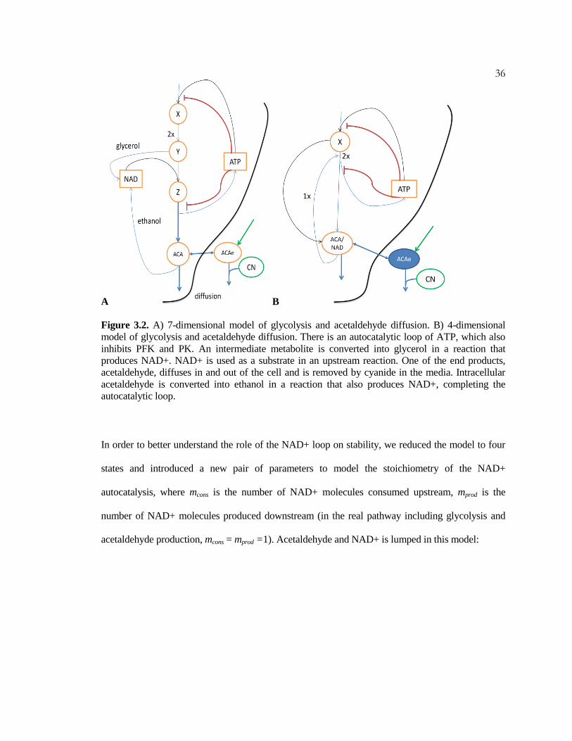
Figure 3.2. A) 7-dimensional model of glycolysis and acetaldehyde diffusion. B) 4-dimensional
model of glycolysis and acetaldehyde diffusion. There is an autocatalytic loop of ATP, which also
inhibits PFK and PK. An intermediate metabolite is converted into glycerol in a reaction that
produces NAD+. NAD+ is used as a substrate in an upstream reaction. One of the end products,
acetaldehyde, diffuses in and out of the cell and is removed by cyanide in the media. Intracellular
acetaldehyde is converted into ethanol in a reaction that also produces NAD+, completing the
autocatalytic loop.
In order to better understand the role of the NAD+ loop on stability, we reduced the model to four
states and introduced a new pair of parameters to model the stoichiometry of the NAD+
autocatalysis, where mcons is the number of NAD+ molecules consumed upstream, mprod is the
number of NAD+ molecules produced downstream (in the real pathway including glycolysis and
acetaldehyde production, mcons = mprod =1). Acetaldehyde and NAD+ is lumped in this model:

37 Figure 3.3. Stability of the 7-
state model. The area in red
shows the parameter region
where the system is oscillating,
while the area in white is where
the system is stable. Just like in
the Kloster model, the system
goes into limit cycle as density is
increased. At lower density the
system moves from stable to
oscillating to stable as the
acetaldehyde removal rate is
increased.
2
2
2
2
2
2
1
(1 )2
1
2( )
1
( )
2
1
2
1
gg
g
prod cons g out in e cg
e out in e cyan e
a
h
a
h
A kXCX k X
A
q kXC AA q
A
kXCC m m k X k C k C d
A
C k C k C k C
V
A
V
A
(3.3)
In this model, since NAD+ is lumped with acetaldehyde, kin encapsulates both the diffusion and the
ethanol reaction, therefore in outk k . As in Chapter 2, we fixed the steady state value of A=1, and
linearize the system to:
( ) 0
(1 ) ( ( ) ( 1) ) (1 ) 0
( ) ( ) ( )
0 0
ee
g ss
ss ss
prod cons ss g prod cons out prod cons ss in
out in cyan
XX
AAA
CC
CC
kC k V a h g kX
q kC V q a h q g q kXA
m m kC k g m m V k m m kX k
k k k
(3.4)
Where Xss and Css are the steady state values of X and C, respectively.
0
0.05
0.1
0.15
0.2
0.25
0.3
0.35
0.4
Density
Ace
tald
eh
yd
e R
em
ova
l Ra
te

38
First, we take 1consm . When mprod=1, which is the value in the real pathway. We can find a
parameter set such that we achieve the desired behavior (Fig 3.4). We asked if it was indeed the
extracellular acetaldehyde concentration that is important for oscillation, as suggested in (32), and
looked at the concentration values in both the stable and the oscillatory regions.
Figure 3.4. Stability regions of the 4-state
glycolysis model with mcons=mprod=1. The
red shows the limit cycle region while white
is the stable region. The plot shows that the
system goes from a stable state to a limit
cycle as the density is increased.
Additionally, at lower density the system
can go from stable to limit cycle and back to
a stable state with increasing acetaldehyde
removal rate. Parameters used were a=1;
h=3; g=1; q=1; V = 4.0136;k =6.0459;
kg=0.5927; kin = 1.0492; kout = 3.1639;
kc=4.7862;
There is in fact no specific range of extracellular acetaldehyde concentration that pinpoints if the
system would oscillate. That is, while there does seem to be a minimum required concentration of
acetaldehyde to affect the glycolytic reactions and induce oscillations, the maximum concentration
in the oscillatory region is actually higher than the maximum in the stable region, thus there is no
range where the system always oscillates (Fig 3.5).
10
Density (alpha)
Ace
tald
eh
yd
e R
em
ova
l R
ate

39 Figure 3.5.
Extracellular acetaldehyde concentration
(Ce) spanning a range of densities and
acetaldehyde removal rates. The left shows
the concentrations found in a stable
parameter set (black) while the right shows
concentrations for parameter sets where the
system oscillate. The system does not
oscillate when [Ce] is too low but there is no
range of extracellular concentration that
determines if the system will always
oscillate.
This result can be easily tested experimentally by adding a flow of acetaldehyde to the extracellular
medium of cells and checking if varying this concentration will change the cellular behavior (most
studies have tried adding pulses of acetaldehyde, which only changes the concentration transiently
(29, 37)). In (27) it is shown that the addition of acetaldehyde did not abolish oscillations, which
supports our results above, but the acetaldehyde concentration added needs to be systematically
varied.
Interestingly, the same parameter values used in Fig 3.4 makes the system oscillatory even in low
density for mprod>2, even though it means lower autocatalysis (Fig 3.6A). Changing the
acetaldehyde removal rate also does not change the effects of the autocatalysis (Fig 3.6B). When we
look at the stability using different parameter values, we find that mprod =mcons is indeed the most
robust (Fig 3.7). This is a surprising result, as we expected that lower autocatalysis (mprod >mcons)
would be more stable, yet in line with the real biological network. It is, however, true that while the
system may oscillate with lower autocatalysis, it is more unstable (unstable node) at higher
autocatalysis.
Stable Oscillatory0
0.05
0.1
0.15
0.2
0.25
0.3
0.35
0.4
0.45
0.5
Extr
ace
llu
lar
Ace
tald
eh
yd
e C
on
ce
tra
tio
n
40
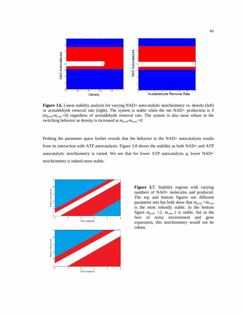
Figure 3.6. Linear stability analysis for varying NAD+ autocatalytic stoichiometry vs. density (left)
or acetaldehyde removal rate (right). The system is stable when the net NAD+ production is 0
(mprod-mcons=0) regardless of acetaldehyde removal rate. The system is also most robust in the
switching behavior as density is increased at mprod-mcons=0.
Probing the parameter space further reveals that the behavior in the NAD+ autocatalysis results
from its interaction with ATP autocatalysis. Figure 3.8 shows the stability as both NAD+ and ATP
autocatalytic stoichiometry is varied. We see that for lower ATP autocatalysis q, lower NAD+
stoichiometry is indeed more stable.
Figure 3.7. Stability regions with varying
numbers of NAD+ molecules and produced.
The top and bottom figures use different
parameter sets but both show that mprod =mcons
is the most robustly stable. In the bottom
figure mprod =2, mcons=1 is stable, but in the
face of noisy environment and gene
expression, this stoichiometry would not be
robust.

41
Figure 3.8. How stability changes with the
interaction of the two autocatalytic loops. NAD
stoichiometry gives the net number of molecules
produced (mprod -mcons), which is 0 in the real
pathway. For q=0, lower NAD stoichiometry is
stable but becomes unstable at higher q.Red is the
oscillatory region and blue is the unstable region.
The Role of Glycerol Production
In glycolysis, the six-carbon sugar fructose-1,6-bisphosphate is cleaved into two three-carbon
sugars, dihydroxyacetone phosphate (DHAP) and glyceraldehyde-3-phosphate (G3P), which can be
interconverted by an isomerase. G3P goes on along the glycolytic pathway to eventually produce
pyruvate and ATP, while DHAP is either converted into glycerol or converted back to G3P. As
discussed above, in anaerobic conditions yeast cells ramp up glycerol production in order to oxidize
NADH to NAD+ and maintain redox balance. Deleting the enzyme glyceraldehyde-3-phosphate
dehydrogenase, which produces NAD+ along with glycerol-3-phosphate eliminates oscillations
(38). It is also known that mutant cells which cannot synthesize glycerol cannot survive in
anaerobic conditions.
When there is no glycerol production at all, or kg=0, the model (3.3) actually has no positive steady
state. To see what role (other than maintaining redox balance) changing the rate of glycerol
production has on the pathway, we also looked at the stability as glycerol production rate is
increased. Fig 3.9 shows that increasing glycerol production rate allows stability for different
0 0.5 1 1.5 2 2.5 3-3
-2
-1
0
1
2
3
ATP autocatalysis (q)
NA
D s
toic
hio
me
try

42 autocatalytic stoichiometry of both NAD+ and ATP. Plotting the stability regions of glycerol
production rate kg vs. other parameters, including density and acetaldehyde removal rate showed
that the system oscillates at low kg but is stable at higher kg, indicating that kg indeed confers
stability. This is interesting, as our model does not impose redox balance constraints, yet increasing
glycerol production not only helps maintain redox balance but apparently also stabilizes the system.
Glycerol production branches off the glycolytic pathway and consumes DHAP, therefore increasing
glycerol production decreases the downstream output (including ATP). This presents another
tradeoff between robustness (stability) and efficiency (ATP output per glucose).
Figure 3.9. Higher glycerol production rate stabilizes a wider range of both ATP (left) and NAD+
(right) autocatalytic stoichiometry. The blue region is unstable while the red region is oscillatory.
The white region shows the stable region.

43 C h a p t e r 4
RIBOSOME AUTOCATALYSIS
Equation Section (Next)
Ribosome synthesis is another significant autocatalytic loop in a cell. Ribosomes are required to
synthesize peptides and proteins, but are also partially composed of proteins themselves, thereby
creating an autocatalytic loop. As we have seen in the previous chapters, autocatalysis can produce
undesirable behavior, such as oscillation or fluctuation. Is there a similar consequence to
autocatalysis in the case of ribosomes? Ribosome concentration is known to have low noise level
(39). Changes in ribosome concentration can drastically affect the protein expression level even
when mRNA levels are constant, and computational studies suggest that in some cases it may even
lead to ultrasensivity (40). Fluctuations in the ribosome level therefore can lead to extremely noisy
protein expression and can be detrimental to the cell.
This loop also presents the problem of resource allocation. Would the cell benefit more from
allocating ribosomes to make more ribosomes, or to make other types of proteins? Is there an
optimal ratio, and how is this ratio controlled? The cell devotes a significant amount of resources to
ribosome production. Ribosomal mRNA transcription accounts for about 50% of the RNA
Polynomerase Pol II transcription in yeast (41) while Pol I transcribes ribosomal RNA (rRNA)
exclusively.
As it turns out, the feedback regulation of ribosome synthesis is still unclear, with various
conflicting models proposed in the literature. One regulation is widely accepted, however. Since
ribosomal proteins must combine with rRNA to form a complete ribosome, the synthesis rate of
both must be regulated to minimize wasteful production of either. Excess ribosomal proteins (that

44 are not complexed with rRNA) inhibit ribosomal protein translation by inhibiting the binding of
ribosomes (42). How the rRNA synthesis is regulated is still under debate, but it is known that
rRNA synthesis responds to the nutrient level (43).
We will explore some of the proposed mechanisms of ribosome regulation, which have included:
1) Free (non-translating) ribosome inhibits the transcription of rRNA via an “indirect”
mechanism. This is called the “ribosome feedback model” (44).
2) The transcription of some rRNA operons is not specifically regulated, but the transcription
rate per operon decreases as the number of rRNA operons (or the number of genes
transcribed) increase because of RNA Polymerase availability goes down, presenting yet
another resource competition problem (43).
3) ppGpp level increases during amino acid deprivation and induces transcriptional pausing of
RNA polymerase, thereby decreasing transcription rate. Another study suggests that rrna
operons are always saturated and higher ppGpp level frees up RNA polymerase to
transcribe unsaturated promoters such as biosynthetic enzymes (45). In this case there is no
feedback from ribosome, but the synthesis rate is controlled by nutrient level.
Minimal Model of Ribosome Synthesis: Resource Competition
The simplest model of ribosome synthesis is a 2-state model of ribosome and non-ribosomal
proteins. Ribosomes are used to produce both species at a ratio v and (1-v), with feedback required
to obtain steady state. Here kt represents the total translation rate, determined by both the translation
rate and the total mRNA level. We assume that the total mRNA level is conserved (due to a limited
pool of RNA Polymerase) and thus the ratios of ribosome and the rest of the proteins sum up to 1

45 (in the next section we explore a larger dimensional model allowing arbitrary expression of both
mRNAs and show that the ratio is indeed what is important).
(1 )
tr
t p
vk RR d R
K R
p v k R d p
(4.1)
When ribosome feedback on ribosome production is implemented, this model correctly captures the
approximate ratio of 50% ribosome production during maximal growth. The protein steady state
level is given by:
(1 ) t rss t
r
vk d Kp v k
d
(4.2)
And we can now solve for the optimal ratio v by solving for 0p
v
, and obtain:
2
t roptimal
t
k d Kv
k
(4.3)
The steady state protein level at this optimal ratio is given by:
2( )
4
t rss
p
k d Kp
d
(4.4)
The second derivative
22
22 0t
p
kp
v d
, therefore by the second derivative test, (4.4) is a local
maxima. During maximal cell growth, ribosomes have been shown to be stable for many hours,
therefore dr is very small (46). We can see that as drK<<kt , voptimal0.5, which corresponds to the

46 observed 50% transcription of ribosomal proteins. The cell grows and divides when it reaches a
certain size, therefore it may never reach steady state. Instead of maximizing for steady state protein
level, it may be more relevant to optimize for growth rate instead. Fig 4.1 shows the optimal
riboprotein transcription ratio for maximal protein synthesis rate at a shorter time scale. This ratio
also lies between 55% to 60% for this 2-state model for various values of kt and dr.
Figure 4.1.
Growth rate (short term protein level)
with varying ribosome production ratio
shows that the optimal ratio lies between
55%-60%. The three curves show the
growth rates for varying kt and dr values.
On the other hand, during starvation translation slows down due to limited amino acid supply and
ribosomes are degraded fast, so the optimal ratio increases as kt decreases and dr increases. Linear
stability also shows that the system is stable when r
t
Kdv
k (there is in fact no positive steady state
beyond this boundary). When nutrient level is low, translation rate (kt) decreases, so v must be
larger (especially since dr is known to increase) and v is no longer optimal (at the optimal ratio the
system is stable when tr
kd
K ). Production of most proteins is halted when the cells are starved,
other than the stress response systems, yet ribosomes are still being produced at a significant rate.
When growth rate drops by 20%, protein levels drop accordingly and the mRNA level drops to 10%
compared to the level during fast growth, but ribosome level only drops to little less than half (47).
0 0.2 0.4 0.6 0.8 10
Ribosome Production Ratio
Gro
wth
Ra
te

47 In starved vibrio cells (after 24 hours of starvation), ribosomes make up around 80% of the total
dry cell mass (48). After 3 days of starvation, this ratio drops to about 50%. We assume similar
numbers will be found in E. coli. This simple model does not explain why ribosome degradation
would increase. Additionally, the model does not really capture the autocatalytic “consumption” of
ribosome (via binding to riboprotein mRNA).
Higher Order Model of Ribosome Synthesis
To capture both resource allocation and autocatalysis, we modeled the production of ribosomes and
“proteins” and ribosomal binding to mRNA. As a first cut, the system was simplified by removing
rRNA, resulting in a 6-state model (Fig 4.2). Both the mRNA of riboproteins (Rm) and mRNA of
the other proteins (Pm) complex with ribosomes (R) and then translated to produce ribosomes and
proteins (P).
We implemented the “ribosome feedback model” discussed above. Since rRNA is not explicitly
modeled, effectively the free ribosomes that are not translating inhibit the synthesis of more
“ribosomes” (ribosomal protein) with strength h.
Figure 4.2. Diagram of the 6-state ribosome synthesis model. mRNAs bind to free ribosomes to
form a complex which dissociates when translation is completed. Free ribosomes inhibit binding to
riboprotein mRNA.

48
( )
1 ( )
( )
( )
1 ( )
( )
on R p m
m rm r R m mh
R p
m pm on R p m p P m m
on R p m
R r Rh
R p
P on R p m p P
r R r
p P p
k R C C RR v k C d R
R C C
P v k R C C P k C d P
k R C C RC k C
R C C
C k R C C P k C
R k C d R
P k C d P
(4.5)
Rm Concentration of mRNA of
riboproteins
vrm Rate of riboprotein mRNA
synthesis
Pm Concentration of mRNA of other
proteins
vpm Rate of other mRNA synthesis
CR Complex of ribosomes bound to Rm kon Binding of ribosomes to mRNA
CP Complex of ribosomes bound to Pm kr, kp Translation rate of ribosomes or
other proteins, respectively
R Concentration of ribosomes dm
dr, dp
Degradation rates of mRNA,
ribosomes, and other proteins,
respectively.
P Concentration of other proteins h Strength of inhibition of free
ribosomes on binding rate.
Table 4. Parameter definitions of model (4.5).
Tradeoffs in Ribosome Synthesis: Maximal Growth and Efficiency
In fast growing E. coli, ribosome composes about 25% of the dry cell mass and ribosomal proteins
make up 50% of Pol II transcription (41). Other than maintaining stable response as discussed
above, is there an optimal ratio of ribosome vs protein synthesis?
Snoep et al used a simple model to look at the optimal ribosome concentration for maximal (steady
state) growth but not the ribosome:protein ratio (49). However, ribosome and protein synthesis is
costly to the cell. If we assume there is a limit to resources inside the cell (e.g. due to saturated
glucose transporter), then the ratio between the two production instead of absolute ribosome
synthesis becomes the variable to optimize.

49 Using the 6-state model above, we looked at the steady state protein concentration spanning
different ratios of ribosome production. We also looked at the relative proportion of ribosomes vs
proteins by mass to define efficiency, corrected for the fact that the average protein is ten times
larger than ribosomes. Fig 4.3 shows that the optimal ratio for growth occurs around 50% ratio of
ribosome transcription, while the proportion in the cell increases with increasing ratio.
Figure 4.3. The optimal
ratio for growh (left) and the
proportion of ribosome in
the cell (right) with
increasing ratio of
transcription devoted to
riboprotein mRNAs.
Tradeoffs in Ribosome Synthesis: Feedback and Stability
Unlike glycolysis, autocatalysis in the case of ribosome synthesis is not as easily quantified. We
can quantify it by the amount of protein needed to form a ribosome, which depends on both the size
of the ribosome and the ratio of ribosomal proteins to rRNA. Higher ribosome to protein production
ratio means higher autocatalysis, and this can result from increased transcription of riboprotein
mRNA compared to protein mRNAs, so one measure of autocatalysis is the ratio of the two
transcription rates vrm:vpm (with the simplifying assumption that the ribosomes bind equally strong
to both types of mRNAs).
0 0.5 10
Ratio of Ribosome Transcription
No
n-r
ibo
so
ma
l P
rote
in
Optimal Ratio for Growth
0 0.5 10
0.1
0.2
0.3
0.4
0.5
0.6
0.7
0.8
0.9
1
Rib
oso
me
/To
tal P
rote
in
Proportion of Ribosome in the Cell

50 By linearizing the model (4.5) we can look at the stability boundaries. Fig 4.4A shows that the
ratio vpm:vrm (and thus the slope in the plot) must stay within a certain range for the system to have a
smooth and stable response. Simulations of the full nonlinear system exhibit this behavior, as shown
in Fig 4.5A. When vrm becomes too high, the system starts to exhibit damped oscillations (Fig
4.5B). As discussed above, some mRNAs are ultrasensitive to ribosome concentration and this
fluctuation could be detrimental (40). When vpm:vrm becomes too high the system crashes, and as it
decreases the system oscillates or goes unstable (Fig 4.5C).
Fig 4.4B shows a similar plot for a higher feedback inhibition. While the boundary locations vary as
the parameter values change, the shape and thus the general tradeoffs remain the same.
Additionally, we also see that higher feedback gain actually narrows the parameter region where the
system has a stable, smooth response.
Figure 4.4. Stability regions as riboprotein mRNA production rate vrm and protein mRNA
production rate vpm are varied. The white region is where the system is stable, blue indicates the
region of damped oscillation, red indicates a limit cycle, and green indicates unstable region. The
plot on the right shows that the stable region is narrowed when h is higher (h=3 compared to h=2
on the left).

51
Figure 4.5. Simulation of model (4.5) as the ratio vrm/vpm is increased. A higher ratio eventually
leads to oscillations (C).
Since higher feedback gain narrows the stable parameter region, we hypothesized that higher
feedback must trade off with another desired property, for example error and sensitivity. We then
looked at the relative changes in the steady state protein and ribosome concentrations to
perturbations in parameter values. We found that higher feedback indeed confers higher robustness
in steady state values to various parameter perturbations (Fig 4.6).
Ribosome Synthesis During Starvation
Production of most proteins is halted when the cells are starved, other than the stress response
proteins. When growth rate drops by 20%, protein levels drop accordingly, and mRNA level drops
to 10% compared to the level during fast growth, but ribosome level only drops to little less than
half (47). In starved vibrio cells (after 24 hours of starvation), ribosomes make up around 80% of
the total dry cell mass (48). After 3 days of starvation, this ratio drops to about 50%. We assume
similar numbers will be found in E. coli. The mRNA levels for a large number of ribosomal protein
genes (in yeast) are reduced by a factor of 2 to 4 during amino acid starvation (50).

52
Figure 4.6. The relative change in steady state level following 10% perturbations in different
parameters for low feedback inhibition (h=1) and high feedback inhibition (h=2). Higher feedback
increases steady state robustness to parameter perturbation.
We modeled starvation conditions by reducing the transcription and translation rates and again
looking at the optimal ratio for growth. The optimal ratio increases somewhat compared to the
maximal growth condition and the proportion of ribosome in the cell is much higher at around 55%
(Fig 4.7), comparable to the numbers seen in vibrio.

53 Figure 4.7.
The optimal ratio for
highest non-ribosomal
protein level increases
in starvation condition
and the proportion of
ribosome in the cell is
much higher. Low
ratio of ribosome
transcription is no
longer stable in
starvation.
While ribosome production is also decreased in starved cells and rRNA transcription by Pol I is
nutrient limited (51), ribosomes are still being produced at a significant rate. Instead of being used
to translate mRNAs, these ribosomes are selectively degraded at an increased rate so that their
amino acid components can be recycled. This seems wasteful, as ribosome production requires
energy which the cell must use sparingly in starvation; so why do the cells continue to produce
significant amounts of ribosome?
One obvious hypothesis is that because the transcription and translation process is slow, when the
cell continues to produce ribosomes, it will be able to respond faster when it suddenly encounters
more nutrient. Indeed, simulation of our model shows that this is indeed the case (Fig 4.8). A
natural extension of the model should include the amino acid recycling from the degraded
ribosomes and proteins, another autocatalytic loop when combined with biosynthetic pathways that
is of interest for future studies.
0 0.5 10
Ratio of Ribosome Transcription
No
n-r
ibo
som
al P
rote
in
Optimal Ratio in Starvation
0 0.5 10
0.1
0.2
0.3
0.4
0.5
0.6
0.7
0.8
0.9
1
Rib
oso
me
/To
tal P
rote
in
Proportion of Ribosome in the Cell
unstable
unstable

54
Figure 4.8.
Simulation of model (4.5)
shows that when the system
keeps a high ribosome
production (high vrm) it
responds faster at the shorter
time scale.
Three-State Model of Ribosome Autocatalysis
The 6-state model above does not explicitly capture how much protein composes a ribosome. The
protein compositions of ribosomes vary in different organisms, ranging from 25% protein in E. coli
(52) to 60% protein in the thermophilic archaea T. aquaticus (53). We are interested in the potential
trade-offs between ribosome with low vs. high protein content. To explore this issue, we now turn
to a 3-state model explicitly modeling both ribosome and ribosomal proteins. We know that rRNA
level corresponds to nutrient level, therefore the total rRNA level (Rt) is modeled as constant and is
the tuning parameter as we see what happens at different nutrient levels.
( )
( ( ) )1
( ( ) )
(1 )1
free t
mp t on t p rp pg
p
on t p r
mt pg
p
rR R S q R
rR k R k q R S q R R d R
R
R k R S q R R d R
rP k R d P
R
(4.6)
In this model we take into account the size of the ribosome, S, and how much of that (q) is
composed of proteins vs. rRNA (S-q). The “ribosome feedback model” proposed by some studies is
0 50 100 150 200 250 300 350
0.4
0.5
0.6
0.7
0.8
0.9
1
Time
[Pro
tein
]
High vrm
Low vrm

55 under debate but we do know that excess ribosomal proteins inhibits translation, which we model
here with coefficient of inhibiton g. Ribosomal proteins bind to free rRNA ( ( )tR S q R ) with
rate kon. Just like in the 2-state model, the total mRNA transcription is also assumed constant and
the control variable is the ratio of transcription between ribosomal protein vs. non-ribosomal protein
mRNAs. First we want to check that this very simple model can recapitulate a well-known
experimental result that the ribosome synthesis rate scales with growth rate, and that the ribosomal
protein transcription ratio (not just the absolute level of transcription) also scales with growth rate
(8). The growth rate is determined by the nutrient level. Fig 4.9 shows that indeed the optimal
transcription ratio rm increases with increasing rRNA level and naturally followed by increasing
protein level.
Figure 4.9. The optimal riboprotein transcription ratio rm increases with increasing nutrient level
(represented by increasing total rRNA, Rt). The growth rate (protein response) increases with
increasing rm and Rt .
Despite the exceeding simplicity of the model, we hope that it can shed light to the effects of
protein content autocatalysis. Analysis of the glycolysis system in Chapter 2 suggests that
00
0.1
0.2
0.3
0.4
0.5
0.6
0.7
Nutrient/rRNA level
op
tima
l rm
0 0.2 0.4 0.60
rm
Pro
tein
Le
ve
l at sh
ort
tim
e s
ca
le

56 autocatalysis can be destabilizing, thus we look at the linear stability of the ribosome synthesis
system with respect to q. The system linearizes to:
2
2
( ) *) ( ) * 0
( ) *)
*(1 * ) 1 *
)(1 * ) 1 *
( ) * 0
* (1
(
(
t on t rp on p
on t on p r
mt m t
mm tg g
p p
g g
p p
p
k k R S q R d k q S q R
k R S q R k S q R d
rk r R
rgr R
k d
R
g
R R
q
q
kR
(4.7)
Figure 4.10.
Stability region with varying
autocatalysis defined by the ribosomal
protein content (q/S) and ribosomal
transcription ratio (rm). As q increases,
higher transcription ratio is needed to
stabilize the system. The region in black
indicates where the system has no
positive steady state, while the region in
green indicates an unstable steady state.
The white region is the stable region.
Fig 4.10 shows the interaction between q and the mRNA transcription ratio. High q (ribosomal
protein content) is destabilizing. As q increases, higher mRNA transcription ratio is needed to
stabilize the system. Increasing ribosomal protein transcription can be costly, however. The
ribosomes are merely machineries required to translate growth and metabolic proteins. An efficient
system should achieve fast growth rate with low amount of ribosomes. Fig 4.11 shows that ratio of
ribosomes (“cost”) over growth proteins (“benefit”) increases nonlinearly with rm.
0 30% 50% 100%0
0.1
0.2
0.3
0.4
0.5
0.6
0.7
0.8
0.9
1
Autocatalysis (q/S)
Rib
oso
me
Tra
nscrip
tio
n R
atio
(R
m)

57
Figure 4.11
The cost of cell growth measured by
the ratio of ribosomes over growth
protein increases with rm. Green dot
indicates that the system is unstable at
that rm.
As discussed before, for a growing cell, growth rate is also an important concern. Simulating the
response of (4.6) shows that higher protein content q is not only destabilizing but also slows down
the response time, leading to slower growth (Fig 4.12).
Figure 4.12. Simulated time response of (4.6) for varying protein content (q/S). The response is
given for all three states: ribosomal proteins, ribosomes, and proteins for protein content=20%,
40%, and 60%. Higher protein content leads to slower response for all three states.
0 20 40 60 800
0.2
0.4
0.6
0.8
1
Co
nce
ntr
atio
n (
no
rma
lize
d to
Ste
ad
y S
tate
)
Ribosomal Protein
0 20 40 60 800.5
0.6
0.7
0.8
0.9
1
1.1
1.2
Time
Ribosome
0 20 40 60 800
0.2
0.4
0.6
0.8
1
Protein
Riboprotein content=20%
Riboprotein content=40%
Riboprotein content=60%
0 0.2 0.4 0.6 0.8 10
0.5
1
1.5
2
2.5
Ribosome Transcription Ratio
R/P

58 While ribosome synthesis scales with growth rate for exponential growth conditions, the system’s
behavior during starvation seems paradoxical. Ribosomes are still produced at a significant rate and
in fact production ratio is much higher in starved cells, yet they are degraded much faster (47). The
fast degradation is not due to a global destabilization of proteins for amino acid recycling, but
selective degradation of ribosomes has been shown to occur through autophagy in starved yeast
cells (54). It seems exceedingly wasteful to produce high level of ribosomes only to be degraded,
but linear stability analysis proposes a possible answer why the cell behaves this way. Fig 4.13
shows the lowest stable rm for varying total rRNA level, Rt. At low Rt (and thus low nutrient level),
the ribosome transcription ratio must be high for the system to be stable.
Figure 4.13.
The minimal ratio for stability decreases as total
rRNA level increases.
The strength of the riboprotein feedback on translation (g) can help stabilize lower transcription
ratios and therefore achieve a higher protein steady state level, as shown in Fig 4.14. Depending on
the parameter values the optimal ratio for highest steady state level may not be stabilized with a
biologically reasonable feedback strength but a lower ratio closer to the optimal will result in a
higher protein level.
00.1
0.2
0.3
0.4
0.5
0.6
0.7
0.8
0.9
rRNA level
Rib
oso
me
Tra
nscrip
tio
n R
atio
Lowest Stable Ratio

59
Figure 4.14.
The blue line shows the optimal
ribosome transcription ratio for
maximal protein level, purple shows
optimal ratio for maximal short term
growth, while the red line shows the
minimum ratio for stability. As the
feedback on riboprotein translation
is increased, the minimum ratio for
stability is decreased while the
optimal ratio is not significantly
affected.
We’ve seen that autocatalysis in the form of ribosomal protein content can make the system
unstable. Fig 4.15 shows that it also affects the optimal transcription ratio for highest steady state
level. Both the optimal and the minimum stable ratio increases with autocatalysis, but it increases
faster for stable ratio. At low autocatalysis it may be possible to operate at the optimal ratio because
it is within the stable range but as autocatalysis increases, the optimal ratio is no longer stable.
Figure 4.15.
The optimal and minimum stable
ratio as autocatalysis is increased.
The optimal transcription ratio in
blue maximizes protein steady
state level, while the ratio in
green maximizes growth rate for
a shorter time scale.
0 0.3 0.5 10
0.2
0.4
0.6
0.8
1
Autocatalysis (q/S)
Rib
oso
me
Tra
nscrip
tio
n R
atio
(rm
)
Optimal Ratio for Highest Steady State
Optimal Ratio for Short Term Growth
Minimal Ratio for Stability
0 1 2 3 4 5 6 7 8 9 100
0.1
0.2
0.3
0.4
0.5
0.6
0.7
0.8
0.9
Riboprotein Feedback Gain (g)
Rib
oso
me
Tra
nscrip
tio
n R
atio
Minimum Stable Ratio
Optimal Ratio for Highest Steady State Level
Optimal Ratio for Max Short Term Growth

60 Thus far we have only looked at feedback as inhibition on translation. Recall the Bode integral
formula and sensitivity function from Chapter 2. Just like the case of glycolysis, we can also ask
what the limitations of an arbitrary controller are for the ribosome system. As we have seen in
Chapter 2, even with an arbitrary optimal controller, the regulated system’s performance is still
constrained by properties of the “open loop” system, measurable by the poles (p) and zeros (z) of
the open loop system (g=0).
While the poles are determined by the eigenvalues of the linearized system (4.7) at g=0, the zeros
are dependent on the feedback interconnection. Our three-state model thus far only incorporated the
feedback from excess ribosomal protein on its own translation, a widely accepted regulation, but
there is also the debated “ribosome feedback model” where ribosomes inhibit rRNA transcription.
By looking at z for both feedback interconnections, we can see the fundamental limits of both types
of feedback even when an arbitrary controller is allowed. Figure 4.16 shows how the poles move as
we change the ribosome transcription ratio (rm) and autocatalysis (q/S). Note that when rm is too
low, there is no positive steady state and thus we do not look at p here. The behavior here is just
another representation of Fig 4.10. High autocatalysis destabilizes the system such that it has a
positive/right half plane p and high transcription ratio can stabilize.
The zeros show a similar behavior for both feedback types. Figure 4.17 shows z for the ribosomal
protein feedback on translation. At low rm, z is positive (and complex) and it becomes negative as rm
increases before splitting into two real, negative z’s. The opposite occurs where z is negative for low
autocatalysis and becomes positive as the autocatalysis is higher. Unlike the glycolysis model where
there is always a RHP z whenever q>1, the ribosome system can tolerate a small amount of
autocatalysis. Figure 4.18 shows a similar behavior for the ribosome feedback on rRNA level (Rt).
One of the zeros stay constant with changing parameters, but the other becomes negative as rm

61
Figure 4.16. The poles of system (4.7) when g=0. At low transcription ratio (rm), there is a positive
pole which is stabilized as rm increases. On the other hand, high autocatalysis (q/S) moves one of the
poles to be positive.
increases and becomes positive as autocatalysis increases. All of the results are consistent that high
ribosomal protein content, and therefore high autocatalysis, poses a constraint on not only system
stability but potential performance.
Figure 4.17. The zeros for
system (4.7) with feedback
from ribosomal protein on its
own translation. High
autocatalysis makes the zeros
positive which aggravates
system constraint but is
ameliorated by higher
transcription ratio.
0 0.2 0.4 0.6 0.8 1-2
-1.5
-1
-0.5
0
0.5
1
Autocatalysis (q/S)0 0.2 0.4 0.6 0.8 1
-2
-1.5
-1
-0.5
0
0.5
1
Ribosome Transcription Ratio
Op
en
Lo
op
Po
les
0 0.2 0.4 0.6 0.8 1-2.5
-2
-1.5
-1
-0.5
0
0.5
1
1.5
2
2.5
Autocatalysis (q/S)
0 0.2 0.4 0.6 0.8 1-2.5
-2
-1.5
-1
-0.5
0
0.5
1
1.5
2
2.5
Ribosome Transcription Ratio
Ze
ros

62
Figure 4.18. The zeros of
system (4.7) with feedback
from ribosomes to rRNA level.
The behavior is similar to the
other feedback type where high
autocatalysis makes one zero
positive, aggravating system
constraint, and can be
ameliorated by high ribosome
transcription ratio.
Rather than increasing the ribosome transcription ratio to stabilize the system, we would ideally
stabilize the optimal transcription ratio. Looking at the closed loop transfer function given by:
( )( )
1 ( ) ( )
P sC s
P s H s
(4.8)
where P(s) is the open loop system and H(s) an arbitrary controller we found that for a feedback
going from Rp to translation, any of the three common controllers (proportional, proportional
integral (PI), proportional integral derivative (PID)) can stabilize the system, but that PI and PID
controllers can stabilize the system at lower gains and that PID controller gives a higher gain
margin. The proportional controller can be implemented via a direct inhibition, while PI and PID
controllers will require a mediating sensor that can integrate the signal or sense the rate of change
rather than absolute change of the output.
0 0.2 0.4 0.6 0.8 1-10
-5
0
5
Ribosome Transcription Ratio
Ze
ros
0 0.2 0.4 0.6 0.8 1-10
-5
0
5
10
15
20
Autocatalysis (q/S)

63 Mitochondrial Ribosomes
Over the course of evolution, the mitochondrion has lost most of its genome. Many of the genes
have been incorporated into the nuclear chromosome, yet mitochondria retain some genes,
including the genes involved in ATP synthesis. It has been suggested that this is due to the
requirement for physical association of these genes with the bioenergetic membranes (55). Loss of
proton gradient in the inner mitochondrial membrane leads to apoptosis and thus this must be
controlled tightly (11).
Mitochondrial ribosomes present a strong evolutionary case for the tradeoffs in riboprotein
autocatalysis. Mitochondria retain a portion, but not all, of the DNA required to transcribe
ribosomal components. Part of the ribosomes are transcribed by the nuclear DNA, translated, and
then transported back into the mitochondria while other parts are transcribed in the mitochondria,
and together they are assembled in the mitochondria. Is there an evolutionary advantage to retaining
only part of the ribosome?
While plants and certain protozoa retain a significant number of their mitochondrial ribosomal
protein genes within the mitochondrial genome, only one small subunit of the identified proteins in
the yeast mitoribosome is encoded in the mitochondria (56). Human mitochondrial ribosomes are
about the same size as bacterial ribosomes, but contain half as many RNA and twice as many
protein components. This seems to suggest that there is an advantage to having more protein
components. Indeed, proteins are more versatile and more stable than RNA and can fold to a
structure that is either more stable or performs more accurately than RNA. Whether there’s a benefit
to having higher protein content is as yet, unproven, however. There are only anecdotal
comparisons available, such as in thermophilic archaea. It has been thought that the evolution of
protein-rich ribosomes is an adaptation to higher temperatures, as ribosomes both eukaryotic and

64 thermophilic archaea have higher protein content than bacterial ribosomes (57). Thermophilic
archaea T. aquaticus has ribosomes which are 60% protein and 40% RNA (53).
However, having a protein-rich ribosome would increase the autocatalysis of riboproteins which,
according to our theoretical analysis above, can aggravate the performance of the system. In
humans, mitochondria bypasses this issue by producing all of the mitochondria ribosomal proteins
on cytoplasmic ribosomes and importing into the mitochondria, thus eliminating the autocatalytic
loop (58). In contrast, the rRNAs are produced within the mitochondria. Since the riboproteins must
form a complex with rRNA, the mitochondria can still control the amount of ribosome complexes
being built by controlling rRNA production (similarly, mitochondria control the production of
respiratory complexes by encoding a few core subunits while the rest are encoded by the nucleus).
Ribosome Heterogeneity
Thus far we had assumed that the ribosomal protein stoichiometry is fixed within each organism
and that the cell controls ribosome synthesis through transcription and translation. There is some
evidence, however, that ribosomes are much more complicated and that the ribosomal protein
composition can change in different conditions. In E. coli, it’s been shown that the ribosomal
protein stoichiometry decreases with slower growth rate (59). Yeast in stationary phase has been
shown to have lower amounts of A-proteins in their large ribosomal subunits compared to
exponentially growing yeast (60). It has been suggested that ribosomes with different protein
compositions transcribe different types of mRNAs and presents another layer of regulatory
complexity (61, 62). Our simple model certainly cannot capture the details of this complexity, but
consistent with the observation in E. coli we can show that lower nutrient level (which translates to
lower rRNA level) indeed requires lower ribosomal protein stoichiometry to be stable (Fig 4.19).

65
Figure 4.19
Stability analysis of the 3-state model shows
that at lower rRNA level, the system requires
lower autocatalysis to maintain stability. The
region in green is unstable while white is the
stable region.
While heterogeneity in ribosome protein content in E. coli was first shown in 1975, there had not
been many studies until recently. As our theoretical results have shown on a very simple model,
autocatalysis is destabilizing and lowers system performance, therefore it is possible (and would be
very interesting) that the observed heterogeneity is a way to control the amount of autocatalysis in
different conditions. It also presents a potential approach to experimentally test our minimal model
analysis as more understanding and techniques develop in the future, by manually tuning the protein
content. However, if the different protein subunits are indeed responsible for different subsets of
mRNA, this approach may not be feasible.
Equation Section (Next)
0
40%
100%
rRNA level
Au
toca
taly
sis
(q
/S)

66 C h a p t e r 5
EVOLUTION OF TRANSCRIPTION NETWORK ARCHITECTURE
Power Law Distributions and Scale Free-ness
The degree distribution of biological networks from metabolic to protein-protein interaction
networks to transcriptional networks has often been characterized as scale-free, following a power-
law distribution (63). However, recent literature suggests that these distributions often do not
conform to a power-law distribution upon closer scrutiny (64-66).
Most researchers use the frequency-degree plot to determine the form of the degree distribution, but
it has been shown that this can be misleading, and that the rank degree plot (where rank r(k) is
defined as the cumulative frequency of degree ≤ k) is less ambiguous (64). A node degree sequence
follows a power law distribution if
( )r k ck (5.1)
In the log-log axis, this curve will follow a straight line with slope (
log ( ) log log logr k ck c k ). On the other hand, a node degree sequence follows an
exponential distribution if
( ) kr k ce (5.2)
Which looks linear in the semi-log axis with slope ( log ( ) log logkr k ce c k ).

67 We found clear differences in the degree distributions between the prokaryotic and eukaryotic
transcriptional networks.
We then explored the differences between two network evolution models widely accepted to
simulate protein-protein networks: the preferential linking model (also known as the Yule process)
(67) and the duplication-divergence model (68, 69). While the two models have been reported to
generate power law distributions, here we show that this was not the case. We also explored the
hierarchical network model which generates power law, hierarchical networks, but we discuss how
this model is not biologically relevant. We next combined the preferential linking and the
duplication divergence model in a way that is supported by biological intuition and shows that the
new combined mechanism generates a network with the same properties as seen in bacteria.
Transcription Network Architecture in Bacteria vs. Yeast
We obtained transcriptional regulatory network data for three well-characterized organisms: B.
subtilis (922 genes, 1380 edges) (70), E. coli (1567 genes, 3989 edges) (71), and S. cerevisiae
(4441 genes, 12871 edges) (68). The average out-degree for all the nodes increases from 1.5 in B.
subtilis to 2.4 in E. coli and 2.9 in S. cerevisiae. The average number of target genes a
transcription factor regulates is 8.8 in B. subtilis, 21.1 in E. coli, and 82 in S. cerevisiae. The
average in-degree (the number of regulators per gene) is 1.5 in B. subtilis, 2.4 in E. coli, and 2.9
in S. cerevisiae.
To determine the degree distribution, we used MATLAB to plot the rank-degree, which is less
ambiguous than the frequency-degree plot. The rank-degree distributions of the bacterial
transcription networks seem to follow a power-law distribution which is linear in the log-log axis,
while the yeast network seems to have an exponential distribution instead (linear in the semi-log

68 axis) (Fig 5.1). On the other hand, the in-degree (incoming edges) distributions are exponential
for all three organisms (Fig 5.2).
Figure 5.1. Rank-degree plot of the three transcriptional regulatory networks in log-log axis.
The bacterial network follows a power law distribution as it is linear in log-log, while the yeast
network follows an exponential distribution.
Figure 5.2.
Distribution of the in-
degree of the three
transcriptional networks in
log-log axis. All three
networks have in-degrees
that follow an exponential
distribution.
Table 5 shows the statistics of the three networks. The median of the entire network is zero due to
100
101
102
103
100
101
102
103
Degree
Ra
nk
Yeast
E coli
B. Subtilis

69 the large amount of target genes and this statistics is therefore not useful, but on the other hand
when we remove the target genes and look at only the non-zero nodes (transcription factors), the
statistics are telling. The median to mean to standard deviation ratio of the yeast network roughly
follows the expected ratio for exponential networks (ln(2) ~=1=1). This is not the case for either
of the bacterial network.
MEDIAN MEAN S.D.
B. subtilis – degree 0 1.5 12.21
B. subtilis - indegree 1 1.5 0.98
E. coli - degree 0 2.4 18.29
E. coli - indegree 2 2.4 1.78
S. cerevisiae- degree 0 2.9 21.79
S. cerevisiae – indegree 2 2.9 2.81
NON-ZERO DEGREE NODES ONLY
MEDIAN MEAN S.D.
B. subtilis - degree 2 8.79 28.56
E. coli - degree 6.5 21.11 50.58
S. cerevisiae - degree 52 81.99 82.59
Table 5. Statistics of the three transcription networks. The top table shows statistics of the entire
network which is less useful due to the large amount of target genes (with degree 0). The bottom
table shows only the non-zero degree nodes (transcription factors).
To see if the operon structure is responsible for the power law distribution in bacteria, we lumped
the genes in E. coli into their respective operons, and plotted the degree distribution for the
operon-operon network. We found that the operon-operon network still has a power law degree
distribution, suggesting that the operon architecture is not responsible for the network structure
(Fig 5.3).

70
Figure 5.3. Rank-degree plot of the operon-operon
regulatory network in E. coli shows that the
network still follows a power law degree
distribution.
We computed the clustering coefficients of the nodes and found that they correlate negatively
with the degree of the node, approximately following a scaling law of 1( )c k k , which indicates
a hierarchical structure in each network (Fig 5.4). We separated the transcription factors from the
target genes in the yeast network and computed the clustering coefficients, which revealed no
correlation and indicated that there is no hierarchy in the interactions between transcription
factors, only from transcription factors to target genes.
Figure 5.4. The clustering coefficients of all three organisms are negatively correlated with
degree.
100
101
102
103
10-4
10-3
10-2
10-1
Degree
Clu
ste
rin
g C
oe
ffic
ien
t
B. subtilis
100
101
102
103
10-4
10-3
10-2
10-1
100
Degree
E. coli
100
101
102
103
10-5
10-4
10-3
10-2
10-1
Degree
S. cerevisiae
100
101
102
103
100
101
102
103
Degree
Rank

71 Comparison of Existing Network Generating Models
We then compared the different models of network evolution which have been previously
proposed in the literature and the types of networks each generates, including the preferential
linking model, the duplication divergence model, and the hierarchical network model (72).
The preferential linking model (the Yule process) (67) was simulated as follows:
1) At each time step a new node is added to the network.
2) The new node forms edges to m existing nodes.
3) The edge to node i forms with the probability proportional to the number of existing
edges from node i ( ii
j
j
kp
k
) where kj is the number of edges from node j.
The preferential linking model generates a network with power law distribution, but clustering
coefficients that are independent of the node degree (Fig 5.5). On the other hand, in the real
bacterial networks clustering coefficients scale inversely with the node degree (a property of
scale-free networks). Therefore, while the preferential linking model is generally accepted as a
model to generate power law networks, it does not generate a scale-free, hierarchical network.
This model thus captures part but not all of the properties of the bacterial transcription network.

72
Figure 5.5
The clustering coefficients of the
network generated by preferential
linking/Yule process do not correlate
with degree.
Even though the authors in (69, 73) previously claimed that the duplication-divergence model
generates a power law distribution, we show that the model actually generates networks with
exponential distributions, linear in the log-linear axis as compared to the preferential linking
model which is linear in the log-log axis (Fig 5.6). In addition, the duplication divergence model
does generate a hierarchical network, and could thus explain the evolution of exponential
distributions in yeast, but not in prokaryotes.
We simulated the duplication-divergence model presented in (73) as follows:
1) At each time step, we select a random node i, which is duplicated into i’. The
duplicated node i’ is linked to the same nodes i is linked. With some probability p, a
new link is added between i and i’ to account for the possibility that the two interact.
2) To account for divergence/mutation, one of the links to/from i’ is removed with
probability q.
As discussed above, the preferential linking model fails to generate a scale-free network due to
100
101
102
10-4
10-3
10-2
10-1
k
C(k
)
Preferential linking network:Clustering Coefficient

73 the distribution of clustering coefficients. Ravasz and Barabasi then proposed the hierarchical
network model which generates a scale-free network with power law distribution and clustering
coefficients that scale inversely with the node degree (72).
The hierarchical network model was simulated according to (72) as follows:
1) We start with a fully interconnected network or cluster with five nodes.
2) At subsequent time steps, four replicas of the entire network are duplicated, and
each of the newly formed peripheral nodes are connected to the central node of the original
cluster.
The generating mechanism is non-realistic for biological networks. In this model, the network is
duplicated into four replicas at each time step. Although whole genome duplication events are
widely accepted, there is no evidence that the genome would be duplicated into so many replicas
at one time. Additionally, the peripheral new nodes are automatically connected to the central
node of the original network. Again, there is nothing to support that this would occur in
transcriptional networks. We therefore concluded that while this model generates a network with
the desired characteristics, it is not relevant for biological networks.
A Biologically Relevant Combined Model
While the preferential linking model does not capture the hierarchical nature of the bacterial
transcription network, the duplication divergence model seems to be a fairly reasonable model for
the yeast network. We believe this can largely be explained by the prevalence of horizontal gene
transfers in bacteria, as we will explain later in the next section. We also simulated the evolution

74
Figure 5.6.
Network generated by the preferential
linking mechanism/Yule process follows
a power law degree distribution (linear
in log-log, blue), while the one generated
by the duplication divergence
mechanism follows an exponential
distribution (red).
of a small power law network which then undergoes expansion via duplication divergence, and as
the network expands, the degree distribution tends to exponential distribution (Fig 5.7). This led
us to combine the two mechanisms into one model, as both horizontal gene transfer and gene
duplication occur in the real biological networks.
We hypothesized that horizontal gene transfers in bacteria occur more frequently for target genes
to acquire new phenotypes such as antibiotic resistance, but less for regulators. Our first cut for a
combined model consisted of duplication divergence for new transcription factors and
preferential attachment of new target genes. We simulated this mechanism to generate a network
of ~1500 nodes and around 10% transcription factors, roughly the same numbers for the E. coli
network. This resulted in a network which looks very similar to that of E. coli: a degree
distribution which follows a power law (Fig 5.8) and clustering coefficients which scale inversely
with the degree (Fig 5.9).
The combined network model was simulated as follows:
1) At each time step, we created a new node. 10% of the time we assume this node will
100
101
102
103
100
101
102
103
104
Degree
Rank
Log Log
Duplication Divergence
Preferential Linking

75 be a transcription factor instead of a target node.
2) When creating a new transcription factor, for X% of the time the new node follows
the duplication divergence step, while for 100-X% of the time it follows the preferential
linking mechanism. We simulated this model both for X=100 and X=50. For a new target
gene, we followed the preferential linking mechanism.
Horizontal gene transfer does occur for transcription factors, although the frequency has been
under debate. Using evolutionary distance as the cutoff, Price et al suggests that a large portion of
transcription factors in E. coli, with the exception of global regulators, actually evolved through
horizontal gene transfer (74), while Teichmann and Babu suggests that the majority evolved
through duplication (75).
We then modified the combined model such that half of the transcription factors evolve via
duplication divergence and half via preferential attachment. We show that this model also still
Figure 5.7. A small power-law network is expanded via duplication divergence. Simulation
shows that the expanded network diverges from power law to an exponential distribution.
100
101
102
100
101
102
103
Ra
nk
200 nodes
100
101
102
100
101
102
103
Degree
700 nodes
100
102
104
100
101
102
103
1200 nodes

76
Figure 5.8. Degree distributions of a network simulated using the combined network model with
around 10% transcription factors to mimic E. coli (left). The degree distribution closely follows
that of the E. coli network (right).
Figure 5.9.
The clustering coefficients of the network
generated using the combined mechanism
scales inversely with degrees, just like in the
biological networks.
generates a network similar to that of E. coli, with power law degree distribution and clustering
coefficients that scale.
100
101
102
103
100
101
102
103
Degree
Ra
nk
Simulated Network
100
101
102
103
100
101
102
103
DegreeR
an
k
E. Coli Network
100
101
102
103
104
10-4
10-3
10-2
10-1
Degree
Clu
ste
rin
g C
oe
ffic
ien
ts
Clustering Coefficients of Simulated Network

77 Prokaryotic vs Eukaryotic Regulation
Studies estimate that gene duplicates account for only 30% of the entire yeast genome (76). The
exon/intron structure of eukaryotic genomes allows for duplication and shuffling of protein
domains rather than whole genes. In transcription factors and chromatin binding proteins it was
shown that this was the main method of protein diversification from yeast to humans (77).
Additionally, the eukaryote architecture has adapted other means of regulations. The
combinatorial regulation using transcription factors poses a constraint on the genome size with
respect to the number of transcription factors. There is evidence that, in prokaryotes, the number
of transcription factors scales quadratically to the number of total genes (10). This scaling is
certainly not seen when we go from prokaryotes to higher eukaryotes. The upper limit of any
known bacterial genome is about 9000 genes and is believed to be constrained by the cell size and
metabolism (11). Mattick suggests that eukaryotes have bypassed this size constraint by relying
more on small non-coding RNAs as regulators (78). The proportion of non-coding RNA in the
genome doubles between bacteria and yeast, and more than quadruples between bacteria and
human (non-coding RNA is estimated to account for more than 80% of the human genome and
only about 10% of bacterial genome (79)). Regulatory RNAs therefore seem to be a much more
scalable regulatory architecture than transcription factors.

78 Chapter 6
CONCLUSIONS
Our analysis in glycolysis illustrates the power of control theory to clarify biological phenomena,
and biology to motivate new theoretical directions (80). In this simple model of glycolysis,
oscillation is neither directly purposeful nor an evolutionary accident, but a necessary consequence
of autocatalysis and hard tradeoffs between robustness and efficiency (or fragility and overhead).
Nature has evolved a control structure finely tuned to effectively manage these tradeoffs with
flexibility to adapt to changes in supply and demand, at the cost of higher enzyme complexity.
Consistent with engineering, purposeful complexity in biology is primarily driven by robustness,
not minimal functionality (1), and there are hard tradeoffs that this complexity mediates.
The theory presented here is consistent throughout in highlighting hard tradeoffs, but there are
important differences in the details. While (2.5) is phenomenological and specific to the model in
(2.2), the theory in (2.10-2.13) is more complete, holding for all frequencies and arbitrarily complex
causal controllers, and also applying to other systems. However, (2.13) still requires substantial
phenomenology, since the formulas for z and p depend on assumptions about autocatalysis (q and a)
and enzyme efficiencies and levels (k). This motivates further unification of control theory with
thermodynamics and statistical mechanics, and recent progress is encouraging (81). It also
motivates rethinking how biology overcomes the “causality” limit with various mechanisms that
exploit predictable environmental fluctuations (e.g. circadian rhythms) or provide remote sensing
(e.g. vision, hearing), both of which can greatly mitigate hard limits such as (2.13) (82). In the case
of circadian rhythms, oscillation is not just a side effect, but has the purpose of exploiting
predictable periodicity in the environment.

79 While our minimal model has limited quantitative predictive power, it can still provide
qualitative insights about experiments, such as which parameters to perturb and why extracts
oscillate more easily than isolated cells. To maximize accessibility, we used the simplest possible
model that captures the real system’s essential features, yet facilitates theoretical analysis
connecting network structure with functional tradeoffs, and allowing the results to be carried out
analytically (a model’s scope and fidelity versus ease of theoretical analysis is itself an inherent
tradeoff (83).) The limits can be generalized to various extensions to our model, including a
nonlinear model of arbitrary length (SI-XII in (5), see also (84)) and reversible reactions (SI-XIII in
(5)). The effect of reversibility in the intermediate (PK) reaction depends on PK inhibition strength
g, and can either ameliorate performance limit at the cost of efficiency, or make it worse. The
analysis readily scales to more complex models with appropriate computer-aided design (CAD)
software, but the results are far less accessible.
We extended our minimal model to include the NAD+ autocatalytic loop and diffusion of
acetaldehyde in and out of the cell. The extended model captures the well known density
dependence of oscillations (3) and the single cell oscillatory behavior seen in (32). The interaction
between the two autocatalytic loops of NAD+ and ATP results an interesting behavior. While
higher ATP autocatalysis aggravates stability and performance, the NAD+ loop seems most robust
when the net product equals zero and lower autocatalysis (where the system produces more NAD+
molecules downstream than consumed upstream) did not seem to ameliorate stability. It turns out
that this is due to the interaction with the ATP loop. If ATP autocatalysis was low (or zero), then
lower NAD+ autocatalysis indeed gives higher robustness. In anaerobic conditions, ATP
autocatalysis is high and the net product of the NAD+ autocatalysis is indeed zero, so the system in
fact sits in the most robust parameter region. The cell also increases glycerol production in
anaerobic growth in order to maintain redox balance by replenishing NAD+ (36). I have also shown

80 that the increased glycerol production not only maintains required redox balance but in fact
makes the system more robust. High glycerol production can stabilize the system even for high
autocatalytic stoichiometry and high cell density. In aerobic conditions, both ATP and NAD+
autocatalysis become much lower due to the additional production of both species from the Krebs
cycle and electron transport system, again letting the system move towards a more robust parameter
region.
Another autocatalytic loop universally found in cells is ribosome synthesis. Synthesis of
ribosomal proteins is not only a problem of autocatalysis but also one of resource allocation, or
resource competition. A two-state model can capture the resource allocation problem and we have
shown that the optimal ratio in maximal growth conditions tend to the ratio seen in exponentially
growing cells. A more detailed model showed that the ribosome to protein production ratio must
sit in a certain range for the system to be stable. Additionally, there is a tradeoff between stability
and robustness of the steady state level to perturbations in various parameters that can be
controlled by the strength of a negative feedback loop.
In synthetic biology, the optimal resource allocation is perturbed by the insertion of new genes
(which are typically not needed for cell growth). The expression of unneeded genes have been
found to decrease the production of cellular machineries such as ribosome and RNA polymerase
and thus can lead to reduced growth rate (85). To really understand optimal resource allocation,
we must also take into account production of metabolic enzymes that produce the energy, and
biosynthetic pathway machineries that produce the building blocks (e.g. amino acids) necessary
for transcription and translation, a big issue which we have not touched here. Ultimately, the
ribosome synthesis model should be combined with the glycolysis model and biosynthetic
pathways for a more complete model of cellular growth.

81
We also developed a three-state model that not only captures the resource allocation but also the
autocatalysis in terms the protein content of ribosomes. While our model is very simple, it
produces some results that will hopefully lead to novel experiments and outlook. All the
theoretical results consistently show that high autocatalysis (high protein content in ribosomes)
aggravate not only system stability but also constraints on the optimal possible performance. The
model also suggests that perhaps the seemingly wasteful behavior of producing significant
amount of ribosomes during starvation is necessary for stability. A possible future experiment is
to tune ribosome production in starvation (or various nutrient levels). Ribosome resource
allocation is currently a widely studied topic, but the possible effects of autocatalysis have not
been noticed. We hope that our simple model will spark an interest in this potentially huge effect
for both experimental efforts and more detailed modeling and analysis
Lastly, we looked at how regulatory protocols can result in large scale differences between
organisms. There seems to be a significant shift in the organization of transcriptional regulatory
networks between prokaryotes and eukaryotes, as exemplified by the differences between B.
subtilis and E. coli vs. S. cerevisiae. We believe these changes could be partially explained by the
fact that lateral gene transfers make up a significant portion of the emergence of new genes in
prokaryotes, while eukaryotes evolve new genes via duplication and mutation. In the future we
would need to extend similar analysis to other eukaryotes, but at the moment, only data for
specific modules is available, and there is no reliable source for the transcriptional regulatory
network of the entire organism in eukaryotes (we have shown that the coagulation network in
human also follows an exponential degree distribution, but this data is still unpublished).
The former can be modeled with the rich-get-richer model which generates power law

82 distributions, and the latter follows the duplication-divergence model, which as we showed
here actually generates exponential distributions. Simulating the evolution of a small power law
network by duplication divergence shows that the network eventually tends to an exponential
network as the new nodes follow an exponential distribution. Of course, neither model can
capture the true mechanisms of network evolution, as there are more than just horizontal gene
transfer, gene duplication, and mutation. A comprehensive model will need to capture events
including loss of regulatory links, whole genome duplication, and exon shuffling.

83 BIBLIOGRAPHY
1. Csete M & Doyle J (2002) Reverse engineering of biological complexity. Science 295(5560):1664-
1669.
2. Doyle J, Francis B, & Tannenbaum A (1992) Feedback Control Theory (Macmillan Press, New
York, NY).
3. Richard P (2003) The rhythm of yeast. FEMS Microb Rev 27(554-557).
4. Sel'kov E (1975) Stabilization of energy charge, generation of oscillations and multiple steady states
in energy metabolism as a result of purely stoichiometric regulations. Eur J Biochem 59:151-157.
5. Chandra F, Buzi G, & Doyle J (2011) Glycolytic oscillations and limits on robust efficiency.
Science 333(6039):187-192.
6. Chandra F, Buzi G, & Doyle J (2009) Linear control analysis of the autocatalytic glycolysis system.
Proc American Control Conf, pp 319-324.
7. Yeung E, Kim J, & Murray R (2013) Resource competition as a source of non-minimum phase
behavior in transcription-translation systems. in Submitted to 2013 Conf Decision Control.
8. Zaslaver A, et al. (2009) Invariant distribution of promoter activities in Escherichia coli. PLoS
Comp Bio 5(10):e1000545.
9. Chandra F, Gayme D, Chen L, & Doyle J (2011) Robustness, optimization, and architectures. Eur J
Control 17(5-6):472-482.
10. Mattick J & Gagen M (2005) Accelerating networks. Science 207:856-858.
11. Lane N (2005) Power, Sex, Suicide: Mitochondria and the Meaning of Life (Oxford University
Press, New York).
12. Betz A & Chance B (1965) Phase relationship of glycolytic intermediates in yeast cells with
oscillatory metabolic control. Arch Biochem Biophys 109(3):585-594.
13. Goldbeter A (1996) Biochemical Oscillations and Cellular Rhythms (Cambridge University Press,
Cambridge).
14. Hynne F, Danø S, & Sørensen P (2001) Full-scale model of glycolysis in Saccharomyces
cerevisiae. Biophys Chem 94(1-2):121-163.
15. Termonia Y & Ross J (1981) Oscillations and control features in glycolysis: Numerical analysis of
a comprehensive model. PNAS 78(5):2952-2956.
16. Richter P & Ross J (1981) Concentration oscillations and efficiency: glycolysis. Science
211(4483):715-717.
17. Kloster A & Olsen L (2012) Oscillations in glycolysis in Saccharomyches cerevisiae: the role of
autocatalysis and intracellular ATPase activity. Biophys Chem (165-166):39-47.
18. Kamp G, et al. (2007) Regulatory properties of 6-phosphofructokinase and control of glycolysis in
boar spermatozoa. Reproduction 133:29-40.
19. Marcondes M, Sola-Penna M, & Zancan P (2010) Clotrimazole potentiates the inhibitory effects of
ATP on the key glycolytic enzyme 6-phosphofructo-1-kinase. Arch Biochem Biophys 497(1-2):62-
67.
20. Chernyak V, Pletjushkina O, Izyumov D, Lyamzev K, & Avetisyan A (2005) Bioenergetics and
death. Biochemistry (Moscow) 70(2):240-245.
21. Astrom K & Murray R (2008) Feedback Systems: An Introduction for Scientists and Engineers
(Princeton University Press, Princeton, NJ).
22. Lestas I, Vinnicombe G, & Paulsson J (2010) Fundamental limits on the suppression of molecular
fluctuations. Nature 467(7312):163-164.
23. Bier M, Teusink B, Kholodenko B, & Westerhoff H (1996) Control analysis of glycolytic
oscillations. Biophys Chem 62(1-3):15-24.

84 24. Stahlberg A, et al (2008) Multiway real-time PCR gene expression profiling in yeast
Saccarhomyces cerevisiae reveals altered transcriptional response of ADH-genes to glucose stimuli.
BMC Genomics 9:170-185.
25. Poulsen A, Petersen M, & Olsen L (2007) Single cell studies and simulation of cell-cell interactions
using oscillating glycolysis in yeast cells. Biophys Chem 125(2-3):275-280.
26. Ghosh A & Chance B (1994) Oscillations in glycolytic intermediates in yeast cells. Biochem
Biophys Res Commun 16(2):174-182.
27. Aon M, Cortassa S, Westerhoff H, & van Dam K (1992) Synchrony and mutual stimulation of yeast
cells during fast glycolytic oscillations. J Gen Microbiol 138:2219-2227.
28. Danø S, Madsen M, & Sørensen P (2007) Quantitative characterization of cell synchronization in
yeast. PNAS 104:12732-12736.
29. Richard P, Bakker B, Teusink B, van Dam K, & Westerhoff H (1996) Acetaldehyde mediates the
synchronization of sustained glycolytic oscillations in populations of yeast cells. Eur J Biochem
235:238-241.
30. De Monte S, d'Ovidio F, Danø S, & Sørensen P (2007) Dynamical quorum sensing: Population
density encoded in cellular dynamics. PNAS 104(47):18377-18381.
31. Bier M, Bakker B, & Westerhoff H (2000) How yeast cells synchronize their glycolytic oscillations:
a perturbation analytic treatment. Biophys J 78(3):1087-1093.
32. Gustavsson A, et al. (2012) Sustained glycolytic oscillations in individual isolated yeast cells. FEBS
J 279(16):2837-2847.
33. Weber A, Prokazov Y, Zuschratter W, & Hauser M (2012) Desynchronisation of glycolytic
oscillations in yeast cell populations. PLoS One 7(9):e43276.
34. Lushchak O, Muller S, & Mair T (2006) Comparison of glycolytic NADH oscillations in yeasts
Saccharomyces cerevisiae and Saccharomyces carlsbergensis. Ukr Biokhim Zh 78(5):22-28.
35. Rodrigues F, Ludovico P, & Leao C (2006) Sugar Metabolism in Yeasts: an Overview of Aerobic
and Anaerobic Glucose Catabolism. Biodiversity and Ecophysiology of Yeasts, The Yeast
Handbook, eds Peter G & Rosa C (Springer Berlin Heidelberg), pp 101-121.
36. Nissen T, Hamann C, Kielland-Brandt M, Nielsen J, & Villadsen J (2000) Anaerobic and aerobic
batch cultivations of Saccharomyces cerevisiae mutants impaired in glycerol synthesis. Yeast
16(5):463-474.
37. Danø S, Sørensen P, & Hynne F (1999) Sustained oscillations in living cells. Nature
402(6759):320-322.
38. Williamson T, Adiamah D, Schwartz J-M, & Stateva L (2012) Exploring the genetic control of
glycolytic oscillations in Saccharomyces cerevisiae. BMC Sys Bio 6:108.
39. Mittal N, Roy N, Madan Babu M, & Chandra Janga S (2009) Dissecting the expression dynamics
of RNA-binding proteins in posttranscriptional regulatory networks. PNAS 106(48):20300-20305.
40. De Vos D, Bruggeman F, Westerhoff H, & Bakker B (2011) How molecular competition influences
fluxes in gene expression networks. PLoS One 6(12):e28494.
41. Warner J (1999) The economics of ribosome biosynthesis in yeast. Trends Biochem Sci 24:437-440.
42. Gourse R, Gaal T, Bartlett M, Appleman J, & Ross W (1996) rRNA transcription and growth rate-
dependent regulation of ribosome synthesis in Escherichia Coli. Annu Rev Microb 50:645-677.
43. Dennis P, Ehrenberg M, & Bremer H (2004) Control of rRNA synthesis in Escherichia Coli: a
Systems Biology approach. Microb Mol Biol Rev 68(4):639-668.
44. Jinks-Robertson S, Gourse R, & Nomura M (1983) Expression of rRNA and tRNA genes in E. coli:
Evidence for feedback regulation by products of rRNA operons. Cell 33:865-876.
45. Jensen K & Pedersen S (1990) Metabolic growth rate control in Escherichia coli may be a
consequence of subsaturation of the macromolecular biosynthetic apparatus with substrates and
catalytic components. Microb Rev 54:89-100.

85 46. Piir K, Paier A, Liiv A, Tenson T, & Maivali U (2011) Ribosome degradation in growing
bacteria. EMBO Reports 12:458-462.
47. Cox R (2003) Correlation of the rate of protein synthesis and the third power of the RNA: protein
ratio in Escherichia coli and Mycobacterium tuberculosis. Microbiology 149:729-737.
48. Flardh K, Cohen P, & Kjelleberg S (1992) Ribosomes exist in large excess over the apparent
demand for protein synthesis during carbon starvation in marine Vibrio sp. strain CCUG 15956. J
Bacteriol 174(21):6780-6788.
49. Snoep J, Westerhoff H, Rohwer J, & Hofmeyr J-H (2006) Is there an optimal ribosome
concentration for maximal protein production? IET Syst Biol 153(5):398-400.
50. Moehle C & Hinnebusch A (1991) Association of RAP1 binding sites with stringent control of
ribosomal protein gene transcription in Saccharomyces cerevisiae. Mol Cell Biol 11(5):2723-2735.
51. Rudra D & Warner J (2004) What better measure than ribosome synthesis? Genes & Dev 18:2431-
2436.
52. Sharma M, et al. (2003) Structure of the mammalian mitochondrial ribosome reveals an expanded
functional role for its component proteins. Cell 115(1):97-108.
53. Zeikus J, Taylor M, & Brock T (1970) Thermal stability or ribosomes and RNA from Thermus
aquaticus. Biochim Biophys Acta 204(2):512-520.
54. Kraft C, Deplazes A, Sohrmann M, & Peter M (2008) Mature ribosomes are selectively degraded
upon starvation by an autophagy pathway requiring the Ubp3p/Bre5p ubiquitin protease. Nat Cell
Biol 10(5):602-610.
55. Lane N & Martin W (2010) The energetics of genome complexity. Nature 467:929-934.
56. Graack H-R & Wittmann-Liebold B (1998) Mitochondrial ribosomal proteins (MRPs) os yeast.
Biochem J 329:433-448.
57. Brown J & Doolittle W (1997) Archaea and the Prokaryote-to-Eukaryote Transition. Microb Molec
Bio Rev 61(4):456-502.
58. O'Brien T (2002) Evolution of a protein-rich mitochondrial ribosome: implications for human
genetic disease. Gene 286:73-79.
59. Milne A, Wai-Nam Mak W, & Tze-Fei Wong J (1975) Variation or ribosomal proteins with
bacterial growth rate. J Bacteriol 122(1):89-92.
60. Saenz-Robles M, Remacha M, Vilella M, Zinker S, & Ballesta J (1990) The acidic ribosomal
proteins as regulators of the eukaryotic ribosomal activity. Biochim Biophys Acta 1030(1-3):51-55.
61. Mauro V & Edelman G (2002) The ribosome filter hypothesis. PNAS 99(19):12031-12036.
62. Byrgazov K, Vesper O, & Moll I (2013) Ribosome heterogeneity: another level of complexity in
bacterial translation regulation. Curr Op Microb 16(2):133-139.
63. Jeong H, Tombor B, Albert B, Oltvai Z, & Barabasi A (2000) The large-scale organization of
metabolic networks. Nature 407:651-654.
64. Tanaka R & Doyle J (2005) Some protein interaction data do not exhibit power law statistics. FEBS
Letters 579:5140-5144.
65. Khanin R & Wit E (2006) How scale-free are biological networks. J Comp Biol 13:810-818.
66. Lima-Mendez G & van Helden J (2009) The powerful law of the power law and other myths in
network biology. Mol Biosys 5:1482-1493.
67. Newman M (2005) Power laws, Pareto distribution, and Zipf's law. Contemp Physics 46:323-351.
68. Balaji S, Madan Babu M, Iyer L, Luscombe N, & Aravind L (2006) Comprehensive analysis of
combinatorial regulation using the transcriptional regulatory network of yeast. J Mol Biol 360:213-
227.
69. Ispolatov I, Krapivski P, & Yuryev A (2005) Duplication-divergence model of protein interaction
network. Phys Rev E Stat Nonlin Soft Matter Phys 72:061911.
70. DBTBS (http://dbtbs.hgc.jp/).
71. RegulonDB (http://regulondb.ccg.unam.mx/).

86 72. Ravasz E & Barabasi A (2003) Hierarchical organization in complex networks. Phys Rev E 67:2.
73. Vazquez A, Flammini A, Maritan A, & Vespignani A (2003) Modeling of protein interaction
networks. ComPlexUS 1:38-44.
74. Price M, Dehal P, & Arkin A (2008) Horizontal gene transfer and the evolution of transcriptional
regulation in Escherichia coli. Genome Biol 9:R4.
75. Teichmann S & Babu M (2004) Gene regulatory network growth by duplication. Nature Genetics
36:492-496.
76. Zhang J (2003) Evolution by gene duplication: an update. Trends Ecol Evol 18:292-298.
77. Lander E (2001) Initial sequencing and analysis of the human genome. Nature 409:860-921.
78. Mattick J (2009) Deconstructing the dogma: a new view of the evolution and genetic programming
of complex organisms. Ann NY Acad Sci 1178:28-46.
79. Westhof E (2010) The amazing world of bacterial structured RNAs. Genome Biol 11:108-110.
80. Iglesias P & Ingalls B (2010) Control Theory and Systems Biology (The MIT Press, Cambridge,
MA).
81. Sandberg H, Delvenne J, & Doyle J (2011) On lossless approximations, the fluctuation-dissipation
theorem, and limitations of measurements. IEEE Trans Auto Control 56(2):293-308.
82. Martins N, Dahleh M, & Doyle J (2007) Fundamental limitations of disturbance attenuation in the
presence of side information. IEEE Trans Auto Control 52(1):56-66.
83. Lander A (2004) A Calculus of purpose. PLoS Biol 2(6):e164.
84. Buzi G, Topcu U, & Doyle J (2011) Analysis of autocatalytic networks in biology. Automatica
47:1123-1130
85. Dong H, Nilsson L, & Kurland C (1995) Gratuitous overexpression of genes in Escherichia coli
leads to growth inhibiton and ribosome destruction. J Bacteriol 177(6):1497-1504.