University of Rhode IslandDigitalCommons@URI

Department of Electrical, Computer, andBiomedical Engineering Faculty Publications

Department of Electrical, Computer, andBiomedical Engineering

2018

Limits on GNSS Performance at High LatitudesPeter F. SwaszekUniversity of Rhode Island, swaszek@uri.edu

Richard J. Hartnett

See next page for additional authors

Follow this and additional works at: https://digitalcommons.uri.edu/ele_facpubs

The University of Rhode Island Faculty have made this article openly available.Please let us know how Open Access to this research benefits you.

This is a pre-publication author manuscript of the final, published article.

Terms of UseThis article is made available under the terms and conditions applicable towards Open Access PolicyArticles, as set forth in our Terms of Use.

This Article is brought to you for free and open access by the Department of Electrical, Computer, and Biomedical Engineering atDigitalCommons@URI. It has been accepted for inclusion in Department of Electrical, Computer, and Biomedical Engineering Faculty Publicationsby an authorized administrator of DigitalCommons@URI. For more information, please contact digitalcommons@etal.uri.edu.

Citation/Publisher AttributionSwaszek, Peter F., Hartnett, Richard J., Seals, Kelly C., Siciliano, Joseph D., Swaszek, Rebecca M. A., "Limits on GNSS Performance atHigh Latitudes," Proceedings of the 2018 International Technical Meeting of The Institute of Navigation, Reston, Virginia, January 2018, pp.160-176.Available at: https://www.ion.org/publications/abstract.cfm?articleID=15549

AuthorsPeter F. Swaszek, Richard J. Hartnett, Kelly C. Seals, Joseph D. Siciliano, and Rebecca M. A. Swaszek

This article is available at DigitalCommons@URI: https://digitalcommons.uri.edu/ele_facpubs/58

Limits on GNSS Performanceat High Latitudes

Peter F. Swaszek, University of Rhode IslandRichard J. Hartnett, U.S. Coast Guard Academy

Kelly C. Seals, U.S. Coast Guard AcademyJoseph D. Siciliano, U.S. Coast Guard Academy

Rebecca M. A. Swaszek, Boston University

BIOGRAPHIES

Peter F. Swaszek is a Professor in the Department of Electrical, Computer, and Biomedical Engineering at the Univer-sity of Rhode Island. His research interests are in statistical signal processing with a focus on digital communicationsand electronic navigation systems.

Richard J. Hartnett is a Professor of Electrical Engineering at the U.S. Coast Guard Academy, having retired fromthe USCG as a Captain in 2009. His research interests include efficient digital filtering methods, improved receiversignal processing techniques for electronic navigation systems, and autonomous vehicle design.

Kelly C. Seals is the Chair of the Electrical Engineering program at the U.S. Coast Guard Academy in New London,Connecticut. He is a Commander on active duty in the U.S. Coast Guard and received a PhD in Electrical andComputer Engineering from Worcester Polytechnic Institute.

Joseph D. Siciliano is a senior undergraduate student in Electrical Engineering at the U.S. Coast Guard Academy. Hehas been performing research as part of a collaborative effort to evaluate GNSS performance at high latitudes.

Rebecca M. A. Swaszek is a PhD candidate in Systems Engineering at Boston University. Her research interestsinclude the modeling and control of discrete event systems and optimization theory.

Abstract

As climate change will likely lead to more of a human presence in the higher latitudes, it is important to consider howwell our safety-critical positioning systems work near the poles. The orbits of the GPS (and other GNSS) precludesatellites with high elevation in these regions; hence, it is clear that at least vertical accuracy is impacted. Thispaper characterizes this positioning performance loss by developing lower bounds on GDOP as a function of receiverlatitude. Examples with actual ephemeris data are included for comparison to the bounds.

Introduction

GNSS performance is often described by the Geometric Dilution of Precision, GDOP, a function of the receiver’s andsatellites’ geometry. While users often think of satellites completely covering the sky, the satellites’ orbital planescontrol where they might occur; even when averaged over time and longitude, at all latitudes there are some portionsof the sky which never contain satellites. As an example, Figure 1 shows a sky view of the GPS satellite trajectoriesfor a 24-hour period here in Reston VA (the site of ION ITM 2018, 38.9581◦N, 77.3563◦W ) showing a significantno-satellite zone (or “bald spot”) in the northern sky.

This characteristic is especially significant at higher latitudes, such as might be experienced by vehicles on polartransit routes in these times of climate change. For example, for users near the poles the observed satellites neverachieve elevation above approximately 45 degrees. Since the vertical accuracy is heavily determined by the contri-bution of high elevation satellites, performance is thus limited. To demonstrate this numerically, Figure 2 shows the

Figure 1: Traces of the GPS satellites’ orbits over the conference site for a 24-hour period in October 2017.

0 10 20 30 40 50 60 70 80 90

Latitude

1.65

1.7

1.75

1.8

1.85

1.9

1.95

GD

OP

valu

es

Figure 2: The best GDOP for 7 GPS satellites, averaged over a 24-hour period, versus receiver latitude.

resulting GDOP for the best 7 GPS satellite position solution for a receiver at different latitudes (5 degree incre-ments), averaged over this same day. It appears that once the latitude exceeds about 55◦ the performance decreasesconsiderable (the GDOP increases).

In this paper we characterize this loss of performance with increasing latitude through the development of a lowerbound to GDOP characterized as a function of the number of satellites and the receiver’s latitude. This paperproceeds as follows:

• First, the GDOP performance criterion is briefly reviewed.

• Next, a mathematical characterization of the no-satellite zone, the bald spot, is presented parameterized bythe receiver’s latitude.

• The GDOP bound from [1] is reviewed, citing the impact of the no-satellite zone on it.

• The GDOP bound is modified to take into account the no-satellite zone.

• Finally, some real data is presented showing the utility of the analytical results.

GDOP

GNSS receivers convert the measured satellite pseudoranges into estimates of the position and clock offset of thereceiver. A common implementation of the solution algorithm is an iterative, linearized least squares method.Assuming that pseudoranges from 4 or more non-coplanar satellites are measured, the direction cosines matrix G isformed and used to solve an over-determined set of equations to solve for position and receiver time offset. Using alocal East (e), North (n), and Up (u) coordinate frame, for m satellites this matrix is

G =

e1 n1 u1 1e2 n2 u2 1...

...em nm um 1

in which (ek, nk, uk) is the unit vector pointing toward the kth satellite from the receiver’s location.

Since the pseudoranges themselves are noisy, the resulting estimates of position and time are random variables. Todescribe the accuracy of this solution, it is common to describe it statistically via the error covariance matrix, equal

to(GTG

)−1scaled by the User Range Error, URE [2]. Rather than considering the individual elements of this

covariance matrix, users frequently reduce it to a scalar performance indicator. The most common of these is theGeometric Dilution of Precision, or GDOP, defined as

GDOP =

√trace

{(GTG)

−1}

In words this is the square root of the sum of the variances of the four solution terms (three position variables andthe time offset) without the URE scaling, a measure of the size of the error ellipsoid. Other common reductions ofthe covariance matrix are the Position (PDOP), Horizontal (HDOP), Vertical (VDOP), and Time (TDOP) portionsof GDOP.

It is well known that the GDOP is a function of the satellite geometry; with only a few visible satellites in poor skylocations the GDOP can become quite large. However, for a future with multiple, fully occupied GNSS constellations,it is expected that receivers would select those satellites to track so as to achieve the best possible performance; see,for example, [3, 4]. Hence, we think that an understanding of both how small the GDOP can be (a lower bound)and the characteristics of the constellations that meet that bound are of value in the satellite selection process and,generally, in understanding GNSS performance. Investigating the best possible GNSS satellite constellation withrespect to GDOP is not a new problem:

• It is known that the GDOP is a monotonically decreasing function of the set of satellites employed in thesolution [5]. Specifically, adding an additional satellite reduces the GDOP independent of the sky locationof this extra satellite, even if it lies directly atop one of the original satellites. This monotonicity extends tomultiple constellations except when the new satellite is the first of its constellation [6].

• Minimum GDOP for 4 satellites, with reference to optimizing the tetrahedron formed by their locations, hasbeen considered by multiple authors, see e.g. [7, 8].

• In a recent paper [1] these authors were able to develop an achievable lower bound to GDOP for terrestrialapplications (i.e. satellites restricted to be above the horizon). Letting m represent the number of satellites,this bound is

GDOP ≥

√2√

6 + 7

m=

3.45√m

(1)

The constellations that achieve this bound consist of approximately 29% of the satellites at zenith and theremaining 71% “balanced” around the horizon (balance having a specific mathematical definition, see also [9]).In that same work the bounds were extended to PDOP, to non-zero mask angle, and to multiple GNSSconstellations. In [9] we showed, by example using real ephemeris data, that good GDOP/PDOP performanceresulted from constellations similar to the “best” constellations resulting from the bounds. Recently thesebounds were extended to allow for an additional range measurement (e.g. an altimeter) [10].

To date the results on GNSS performance and the development of satellite selection algorithms have NOT taken intoaccount where on the Earth the user is. While not often discussed, the orbital planes of the satellites limit thoseparts of the sky in which satellites might be visible. For example, users near either of the poles see no satellitesat elevation above about 45 degrees. Combining this with a mask angle of 5 or 10 degrees leaves a narrow ring ofsatellite elevations, limiting vertical accuracy. Even at lower latitudes some portions of the sky are off limits:

• At the equator no satellites are visible at the horizon for ±30 degrees of azimuth around each pole; fortunately,this no-satellite swath only has maximum elevation of about 15 degrees.

• At latitude 40 degrees north (near the conference site in Reston) the no-satellite portion of the sky rises fromthe north pole reaching an elevation of 60 degrees and azimuth of −40 to 40 degrees.

Clearly these regions in the sky where no satellite could possibly be situated will impact possible system perfor-mance.

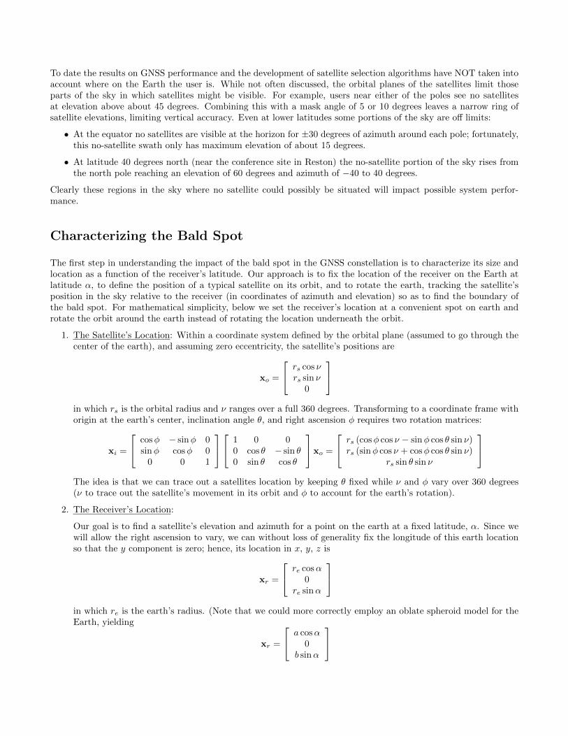
Characterizing the Bald Spot

The first step in understanding the impact of the bald spot in the GNSS constellation is to characterize its size andlocation as a function of the receiver’s latitude. Our approach is to fix the location of the receiver on the Earth atlatitude α, to define the position of a typical satellite on its orbit, and to rotate the earth, tracking the satellite’sposition in the sky relative to the receiver (in coordinates of azimuth and elevation) so as to find the boundary ofthe bald spot. For mathematical simplicity, below we set the receiver’s location at a convenient spot on earth androtate the orbit around the earth instead of rotating the location underneath the orbit.

1. The Satellite’s Location: Within a coordinate system defined by the orbital plane (assumed to go through thecenter of the earth), and assuming zero eccentricity, the satellite’s positions are

xo =

rs cos νrs sin ν

0

in which rs is the orbital radius and ν ranges over a full 360 degrees. Transforming to a coordinate frame withorigin at the earth’s center, inclination angle θ, and right ascension φ requires two rotation matrices:

xi =

cosφ − sinφ 0sinφ cosφ 0

0 0 1

1 0 00 cos θ − sin θ0 sin θ cos θ

xo =

rs (cosφ cos ν − sinφ cos θ sin ν)rs (sinφ cos ν + cosφ cos θ sin ν)

rs sin θ sin ν

The idea is that we can trace out a satellites location by keeping θ fixed while ν and φ vary over 360 degrees(ν to trace out the satellite’s movement in its orbit and φ to account for the earth’s rotation).

2. The Receiver’s Location:

Our goal is to find a satellite’s elevation and azimuth for a point on the earth at a fixed latitude, α. Since wewill allow the right ascension to vary, we can without loss of generality fix the longitude of this earth locationso that the y component is zero; hence, its location in x, y, z is

xr =

re cosα0

re sinα

in which re is the earth’s radius. (Note that we could more correctly employ an oblate spheroid model for theEarth, yielding

xr =

a cosα0

b sinα

with a and b being the equatorial and polar radii, respectively, but observe that there is no observable numericaldifference in the results below.)

This receiver location forms a tangent plane on the surface of the earth. The unit vector

~n =

cosα0

sinα

is normal to this plane and is used below in computing elevation. The unit vector

~a =

− sinα0

cosα

is in this tangent plane and points north and is used below in computing azimuth. Finally, the unit vector

~b =

010

completes an orthogonal coordinate frame with ~n and ~a.

3. The Sky View’s Terms: The difference vector (pointing from the the receiver to the satellite) is

~d = xi − xr =

rs (cosφ cos ν − sinφ cos θ sin ν)− re cosαrs (sinφ cos ν + cosφ cos θ sin ν)

rs sin θ sin ν − re sinα

Let d represent the length of this vector

d = |xi − xr|and dn, da, and db be its projections on the coordinate frame defined by the receiver’s location

dn = ~d · ~n , da = ~d · ~a and db = ~d · ~b

The elevation and azimuth angles to the satellite are trigonometric functions of these projections

elev = sin−1(dnd

)and azi = tan−1

(dbda

)4. The Bald Spot:

By letting ν and φ both range over a full 360 degrees, the expressions above provide the possible elevation andazimuth angles for a satellite on a circular orbit of radius rs and inclination angle θ (assumed constant for allsatellites) as seen by a receiver at latitude α on the surface of the Earth (for points h units above the spheroidwe could add h to re). Figure 3 shows the results for a GPS satellite (rs = 26, 559.7 km, θ = 55◦) and a receiverat the surface of the earth with various latitudes from the equator to the north pole. For these graphics theresolution on ν and φ was 5◦. As expected, receivers at the equator do not see satellites at the horizon directlyto the north or south. With increasing latitude, the bald spot rises from the north pole, eventually becomingdirectly overhead.

Examining Figure 3 we make several points:

• Satellite azimuths and elevations appear to have a continuous range except for one or two generally ovalareas – this can be easily imagined from the figure and becomes more obvious with denser computationover ν and φ.

• Not obvious from the figures, but notable in computation, is that the edge of the northern bald spotresults from ν = 90◦ (the right image in Figure ?? repeats the plot, but with the ν = 90◦ results plottedas blue crosses). Similarly, ν = 270◦ generates the boundary of the southern bald spot, if it exists.

• This images are for a receiver at sea level; as the receiver altitude increases the bald spot grows.

Based on these comments, especially the second, we focus below on the mathematics for ν = 90◦.

Figure 3: Range of visible satellites versus latitude.

5. Characterizing the Boundary:

If ν = 90◦ then the satellite’s position is

xi =

−rs cos θ sinφrs cos θ cosφrs sin θ

Recognizing that the inclination angle, θ, is assumed to be fixed, this location has constant z component whilex and y vary with φ (i.e. the satellite position that forms the bald spot boundary rotates on a plane parallelto the equator).

Continuing, the difference vector is

~d =

−rs sinφ cos θ − re cosαrs cosφ cos θ

rs sin θ − re sinα

with length

d =√r2s + r2e + 2rsre (cosα cos θ sinφ− sinα sin θ)

The three projections are

dn = rs (sinα sin θ − cosα cos θ sinφ)− reda = rs (cosα sin θ + sinα cos θ sinφ)

db = rs cos θ cosφ

Figure 4: Boundaries for latitudes 0, 30, 60, and 90 degrees.

so

elev = sin−1

(rs (sinα sin θ − cosα cos θ sinφ)− re√

r2s + r2e + 2rsre (cosα cos θ sinφ− sinα sin θ)

)and

azi = tan−1(

cos θ cosφ

cosα sin θ + sinα cos θ sinφ

)Figure 4 shows several such boundaries. We observe the expected left-right symmetry and generally oval shape.

6. A Sanity Check:

Consider the situation for a receiver at the north pole, α = 90◦, so that

elev = sin−1

(rs sin θ − re√

r2s + r2e − 2rsre sin θ

)and

azi = tan−1(

cosφ

sinφ

)= 90− φ

Observe that the elevation does not depend upon φ, it is a constant for all azimuths. This elevation is a functionof the satellite’s and earth’s radii, rs and re, as well as the inclination angle θ. Using rs = 26, 559.7, re = 6, 371(both in km), and θ = 55◦, the bald’s spots boundary is perfectly circular at elevation 45.3◦. Similarly, forGalileo with θ = 56◦ and rs = 23, 222 the satellites never appear above elevation 44.8◦. Further, for receiversat higher altitudes this elevation decreases.

7. Azimuths 0◦ and 180◦:

Consider azimuths 0◦ and 180◦ which occur when db = 0 or

rs cos θ cosφ = 0

or φ = ±90◦. The corresponding elevation expression is

elev = sin−1

(rs (sinα sin θ ∓ cosα cos θ)− re√

r2s + r2e + 2rsre (± cosα cos θ − sinα sin θ)

)(2)

which partially describes the extent (height) of the bald spot in the north/south direction. Figure 5 plots thisresult versus latitude α. The upper blue line is the elevation of the leading edge of the bald spot (using the

0 10 20 30 40 50 60 70 80 90

Latitude in degrees

0

30

60

90

60

30

Ele

va

tio

n e

xte

nt

in d

eg

ree

s

leading edge

trailing edge

Figure 5: The extent of the northern bald spot’s boundary at azimuths 0◦ and 180◦.

lower plus/minus signs) as it rises from the north; above latitude of about 55◦ the bald spot passes beyondzenith with the elevation falling toward the south (hence, the non-monotone vertical axis values in this figure).The red line is the trailing edge of the bald spot (the upper signs); it also breaks from the horizon at aboutlatitude 55◦.

Strictly, the bald spot hits zenith when the leading elevation equals 90◦, or

rs (sinα sin θ + cosα cos θ)− re√r2s + r2e − 2rsre (cosα cos θ + sinα sin θ)

= 1

Manipulating the algebra and trigonometry, this is equivalent to α = θ; the leading edge hits zenith when thelatitude is equal to the satellite’s inclination angle.

Similarly, the bald spot breaks off from the horizon when the trailing elevation equals 0◦, or

rs (sinα sin θ − cosα cos θ)− re = 0

Solving for the latitude

α = cos−1(−rers

)− θ

For GPS, this is α = 53.4◦, so the bald spot leaves the horizon just before its leading edge hits zenith.

8. Intersection with the Horizon:

Consider where the bald spot’s boundary hits the horizon; equivalently, where the elevation is 0◦ or theprojection dn is zero

rs (sinα sin θ − cosα cos θ sinφ)− re = 0

We can solve for sinφ

sinφ =rs sinα sin θ − rers cosα cos θ

We also have

cosφ =

√1− sin2 φ

Using this result in the azimuth expression

azi = tan−1

cos θ√r2s cos2 α cos2 θ − r2s sin2 α sin2 θ + 2rsre sinα sin θ − r2e

rs sin θ cos θ − re sinα cos θ

Figure 6 plots this result versus latitude α. For lower latitudes the the intersection with the horizon startsat 30.3◦ for a receiver at the equator, increases and then decreases smoothly with increasing latitude, finallydisappearing (shown here as azimuth equal to zero) for latitudes above 53.4◦.

0 10 20 30 40 50 60 70 80 90

Latitude in degrees

0

15

30

45

Azim

uth

in

de

gre

es

Figure 6: The azimuth of the northern bald spot’s boundary at zero elevation.

A Brief Review of [1]

Following [1] the GDOP under GNSS alone is determined by the elements of the symmetric matrix GTG with

GTG =

m∑k=1

e2k

m∑k=1

eknk

m∑k=1

ekuk

m∑k=1

ek

m∑k=1

eknk

m∑k=1

n2k

m∑k=1

nkuk

m∑k=1

nk

m∑k=1

ekuk

m∑k=1

nkuk

m∑k=1

u2k

m∑k=1

uk

m∑k=1

ek

m∑k=1

nk

m∑k=1

uk m

Finding the minimum of GDOP in [1] was a four step procedure:

1. Set the off-diagonal terms to zero. Strictly we cannot do this for all of these terms; however, setting the onesshown in red (all but the

∑k uk since each uk ≥ 0) is desired. Hence, we want

m∑k=1

ekuk = 0

m∑k=1

ek = 0

m∑k=1

nkuk = 0

m∑k=1

nk = 0

m∑k=1

eknk = 0

Effectively, these are conditions that the satellite constellation exhibit symmetry in multiple directions. In [1]these conditions, along with next one below, are used to define a “balanced” satellite constellation. See [9] fora more detailed discussion of balance.

2. Set the first two diagonal terms (in blue) to be equal to one another

m∑k=1

e2k =

m∑k=1

n2k

We note that it is possible to satisfy all 6 of these conditions for any m greater than 3 if the sky locations areunrestricted (beyond being above the horizon) [9].

3. The impact of the remaining off-diagonal term on GDOP (in black) is minimized by forcing all of the satellitesto be at either zenith or on the horizon (elevations 90◦ and 0◦, respectively); let β represent the fraction of the

m satellites at zenith, then the GDOP bound reduces to

GDOP ≥

√1 + 5β

mβ (1− β)

4. Finally, standard calculus provides the optimum value for β is√6−15 ≈ 0.29 which yields the GNSS-only bound

presented above in Eq. (1).

Including the bald spot we expect a similar result, specifically, of the form

GDOP ≥ C(α)√m

in which the numerator constant depends upon the latitude.

The Bald Spot and the GDOP Bound

To extend the results in [1] for restrictions on satellite locations we consider several cases, depending upon lati-tude:

• α < 55◦: First, consider the case of smaller latitudes, α < θ. In this case the “bald spot” does not includezenith, so the results from [1] hold; the small portion(s) of the horizon restricted due to the no satellite zonedoes not inhibit the horizon satellites from forming a balanced constellation. Specifically, Eq. (1) holds so thatC(α) = 3.45 and the performance is the blue part of the plot of C(α) =

√m×GDOP for this range of α shown

in Figure 7.

• At the North Pole, α = 90◦: Arguments presented in [11] prove that the best GPS satellite constellation for areceiver at the pole is to have satellites limited to either the horizon or elevation θp = 45.3◦. Let γ = sin θp.

0 10 20 30 40 50 60 70 80 90

Latitude in degrees

3.3

3.4

3.5

3.6

3.7

3.8

3.9

4

GD

OP

co

eff

icie

nt

Figure 7: The coefficient of the GDOP, C(α) =√m × GDOP , as a function of latitude α. The blue line is the

original bound for α < 55◦; the red dotted line is a lower bound to the lower bound which clearly indicatesthat the performance gets worse (monotonically) as the no-satellite zone encompasses more of the highelevation region; the red dot is an achievable bound at the pole; the red line is achievable performance forthe conjectured solution.

Assume that βm of the satellites are at this higher elevation, (1− β)m are at the horizon, and that both setsare “balanced” as per [1]. Then from [11] we have that β should be a root of the 4th order polynomial

γ4(γ2 + 4

)β4 − 8 γ4 β3 + 3γ2

(γ2 − 1

)β2 + 2

(γ2 + 1

)β − 1 = 0

and

GDOP ≥

√(4

1− βγ2+

1 + βγ2

β(1− β)γ2

)1

m(3)

Rooting the polynomial yields β = 0.41 (i.e. 41% of the satellites should be at the highest elevation) and

GDOP (90◦) ≥ 3.86√m

a 12% increase in the GDOP coefficient. This appears as the red dot at α = 90◦ in Figure 7.

• Latitude between 55◦ and 90◦ – Part 1:

A non-achievable lower bound can be constructed by shrinking the no-satellite region and applying the resultsfrom [11]. Specifically, consider Figure 8 which shows the situation at latitude 65◦; the pink region is theno-satellite zone. Shrinking this to the circular cap about zenith (shown in red), we can compute the size ofthis cap using Eq. (2) and apply the results of [11]. The result is the red dotted line in Figure 7. As anoptimum satellite constellation for this smaller region would required balanced satellites in the pink region, thebound is generally unachievable.

• Latitude between 55◦ and 90◦ – Part 2

To tighten the bound, consider Figures 9 and 10 (in these and other sky view figures below, the circle anddiamond symbols are meant to show locations for satellites, not individual satellites; for example, the leftmostsky view in Figure 9 could be showing the locations of a 4 satellite constellation, but might also be showinglocations for 8 satellites, two at each spot, the center sky view would be optimum for 6 satellites, 2 at zenithand 1 at each of the other 4 horizon locations):

– The first of these shows possible optimum configurations at latitude 55◦; 29% of the satellites would beat zenith while the remaining 61% are distributed evenly around the horizon (potentially at either 3 or 4locations).

– The second of these shows possible optimum configurations at latitude 90◦; now 41% of the satellites aredistributed evenly at elevation 45.3◦ (2 or 3 locations) while the remaining 59% are distributed aroundthe horizon (evenly for the first two figures; in the last configuration with only two locations at elevation45.3◦, north and south, there would need to be a higher percentage of satellites to east and west to balancethem).

Figure 8: The region for a lower bound to the lower bound.

Figure 9: Some optimum constellations at α = 55◦.

Figure 10: Some optimum constellations at α = 90◦.

Note that there are many other configurations that would achieve the same minimum GDOP at either of theselatitudes (for example, arbitrary rotations of the patterns or more symmetric locations beyond three or four);these choices just help to motivate the constellations considered below. Specifically, as shown in Figure 11 westarted with a generic configuration for latitudes between 55◦ and 90◦:

– Some fraction of the satellites are distributed amongst 4 locations on the boundary of the bald spot, duenorth, due south, and a pair symmetrically east/west; the remaining satellites appear at 6 locations onthe horizon, again divided due north, due south, and to two symmetric east/west pairs of locations.

– The swaths of pink and blue in this diagram are meant to suggest that the azimuths of the east/westpairs (pairs of diamond symbols both on the horizon and the boundary) will be allowed to range over[0◦,±180◦] during an optimization step.

This configuration has 10 parameters:

Figure 11: The generic conjectured constellation.

– Seven fractions m1 through m7 corresponding to the 7 unique locations: (1) boundary south, (2) boundarynorth, (3) boundary east/west (i.e. matching fractions in both directions), (4) horizon south, (5) horizonnorth, and (6,7) two horizon east/west fractions.

– Three azimuths (for the locations on the boundary the azimuth specifies the elevation, for the locationson the horizon the elevations are identically zero).

Constrained numerical minimization of the GDOP over these 10 parameters yields the performance shownas the solid red line in Figure 7; we conjecture that no better configuration of satellites exists. Further, anexamination of the optimum choices for the 10 parameters indicates that the constellation is over parameterized.Specifically the fraction of satellites at horizon north goes to zero and the three azimuths do not change fromtheir initialized values over the course of the optimization. Other (reasonable) initial values for the threeazimuths also yield the same level of performance with different results for the optimized fractions.

This generic constellation can be altered in various ways without impacting the optimum performance. Thesimplest is shown as an inset in Figure 12: two locations on the bald spot boundary (due north and due south)and three locations on the horizon (due south and a symmetric east/west pair). Figure 12 itself shows thefractions of satellites at these locations, the color and symbol choices match the inset diagram; Figure 13 showsthe azimuths:

– The locations on the bald spot boundary starts with approximately 29% of the satellites due south (bluecircles) with 0 due north (red circles) at latitude 55◦ and eventually converge to a combined total of 41%on the boundary at latitude 90◦..

– Interestingly, we don’t need any satellites due north on the bald spot boundary (red circles) until weexceed approximately 70◦ of latitude.

– At latitude 55◦ the 71% of the satellites on the horizon are split evenly across the three locations andthese locations are evenly distributed on the horizon (120◦ spacing); as the latitude increases the optimumvalues for the fractions and the azimuths change somewhat.

In a similar fashion we optimized the performance of several other reductions of the generic configuration

Figure 12: Allocation of satellites (as percentages) for the 5 location constellation versus latitude.

55 60 65 70 75 80 85 90

Latitude

60

65

70

75

An

gle

s

Figure 13: Horizon azimuth for the 5 location constellation versus latitude.

in Figure 11. While these yielded different sets of optimum parameters, we repeat that they all resulted inequivalent GDOP performance !! In other words, there are many possible equivalent minima for GDOP (recallthat for latitudes below 55◦ all that matters is that we put 29% of the satellites at zenith and the remaining71% “balanced” around the horizon – these could be scattered into 3 locations, 4 locations, or more (see [9]).Examples of this, for latitudes 60◦, 70◦, and 80◦ are shown in Figures 14, 15, and 16 (each figure shows threedistinct constellations with the locations and fractions of satellites marked, the leftmost being the simplestconfiguration).

Figure 14: Some optimum constellations at latitude α = 60◦.

Figure 15: Some optimum constellations at latitude α = 70◦.

Figure 16: Some optimum constellations at latitude α = 80◦.

Examples

To compare the developed bounds and conjectured optimum constellations to reality we generated GPS constellationdata for a 24-hour period at multiple locations on the Earth (latitudes 60◦, 70◦, and 80◦ N, 5◦ spacing in longitude)and computed the GDOP for a 7 satellite solution, keeping the best configurations. Figure 17 shows an examplefrom each of these latitudes that mimic the optimum configurations of the above discussion. Specifically, we noticehow three (or four) satellites hug the no-satellite boundary and that the others are near the horizon in a somewhatbalanced configuration.

Figure 17: Real constellations.

Conclusions/Future

We have developed a lower bound to GDOP taking into account the latitude of the receiver and the fact that athigher latitudes the satellites are restricted to be lower in the sky. For parts of the range of latitudes (specifically,0 to 55◦ and at 90◦) the bound is tight (i.e. achievable). For the remainder of the range we have a non-achievablebound and conjecture a second result to be the actual lower bound (both shown in Figure 7).

The lack of high satellites at higher elevation directly impacts vertical accuracy. As an example, Figure 18 repeatsthe GDOP coefficients of Figure 7, but separates out the horizontal, vertical, and time portions of the DOP (theGDOP is the square root of the sum of squares of these components). Quite clear from this figure is that the growthin GDOP for higher latitudes is primarily due to a loss of VDOP performance (the VDOP increases for latitudesabove 55◦ while the HDOP and TDOP remain relatively constant).

0 10 20 30 40 50 60 70 80 90

Latitude

1

1.5

2

2.5

3

DO

P c

oe

ffic

ien

t

HDOP

VDOP

TDOP

Figure 18: Separation of the GDOP into horizontal, vertical, and time portions vs latitude.

References[1] P. F. Swaszek, R. J. Hartnett, and K. C. Seals, “Lower bounds on DOP,” Jour. Navigation, vol. 70, no.5, June

2017, pp.1041-1061.

[2] P. Misra and P. Enge, Global Positioning System: Signals, Measurements and Performance, Massachusetts:Ganga-Jamuna Press, 2nd ed., 2006.

[3] D. Gerbeth, M. Felux, M-S. Circiu, and M. Caamano, “Optimized selection of satellites subsets for a multi-constellation GBAS,” Proc. ION Int’l. Tech. Mtg., Monterey CA, Jan. 2016.

[4] T. Walter, J. Blanch, and V. Kropp, “Satellite selection for multi-constellation SBAS,” Proc. ION GNSS+ 2016,Portland OR, Sept. 2016.

[5] R. Yarlagadda, I. Ali, N. Al-Dhahir, and J. Hershey, “GPS GDOP metric,” IEE Proc. Radar, Sonar, Navig.,vol. 147, no. 5, Oct. 2000, pp. 259-264.

[6] Y. Teng and J. Wang, “New characteristics of geometric dilution of precision (GDOP) for multi-GNSS constel-lations,” Jour. Navigation, vol. 67, 2014, pp. 1018-1028.

[7] M. Kihara and T. Okada, “A satellite selection method and accuracy for the Global Positioning System,” Jour.Navigation, vol. 31, no. 1, Spring 1984, pp. 8-20.

[8] J. J. Spilker, “Satellite constellation and geometric dilution of precision,” Global Positioning System: Theory andApplications Volume 1, 1996, pp. 177-208.

[9] P. F. Swaszek, R. J. Hartnett, and K. C. Seals, “Multi-constellation GNSS: new bounds on GDOP and a relatedsatellite selection process,” Proc. ION GNSS+ 2016, Portland OR, Sept. 2016.

[10] P. F. Swaszek, R. J. Hartnett, and K. C. Seals, “GDOP bounds for GNSS augmented with range information,”Proc. ION GNSS+ 2017, Portland OR, Sept. 2017.

[11] P. F. Swaszek, R. J. Hartnett, and K. C. Seals, “A lower bound to DOP based upon knowledge of the highestand lowest satellite elevations,” in preparation...