linalg ch6 - kaist
TRANSCRIPT

80

Chapter 6
Linear Transformations
6.1 Matrices as Transformations
Definition 6.1.1. A function or a transformation f : Rn → Rm, domain,
image, The set f(Rn) is the range of f . The space Rm is the codomain.
matrix transformation, identity transformation
Example 6.1.2. Consider a transformation T : R2 → R2 determined by one
of the following three conditions:
(1) T maps a vector x = (x1, x2) to T (x) = (x1 + x2, 2x1 − x2)
(2) T maps a vector x = (x1, x2) to T (x) = (2x1, 3x2)
(3) T maps a vector x = (x1, x2) to T (x) = (x21, x2)
Example 6.1.3. Let
A =
0 1
1 2
−2 3
and let TA be a linear transformation T : R3 → R2 determined by the following
TA(x) = Ax.
The component of T is
TA
([
x1
x2
])
=
x2
x1 + 2x2
−2x1 + 3x2
(6.1)
81

82 CHAPTER 6. LINEAR TRANSFORMATIONS
Definition 6.1.4. If for any vector u, v ∈ Rn and scalar α ∈ R, a function
T : Rn → Rm satisfies
(1) T (αu) = αT (u) (Homogeneity)
(2) T (u+ v) = T (u) + T (v) (Additivity)
then we say T is a linear transformation(mapping). In the special case
when m = n, T is called an operator.
Example 6.1.5. Express a given linear transformation T : Rn → Rm using
the standard basis vector.
Since any vector x in Rn can be written as x = x1e1 + x2e2 + · · ·+ xnen,
T is determined by the values of these vectors. Thus we see
T (x1e1 + x2e2 + · · ·+ xnen) = T (x1e1) + T (x2e2) + · · ·+ T (xnen)
= x1T (e1) + x2T (e2) + · · ·+ xnT (en)
= [T (e1)T (e2) · · · T (en)]
x1
x2...
xn
Since T (e1), T (e2), . . . , T (en) are vectors in Rm, we can write it as a linear
combination of e1, e2, . . . , em. Hence there exist numbers tij (1 ≤ i ≤ m, 1 ≤
j ≤ n) s.t.
T (e1) =
t11
t21...
tm1
, T (e2) =
t12
t22...
tm2
, · · · , T (en) =
t1n
t2n...
tmn
(6.2)
In other words,
T (ej) =m∑
i=1
tijei (1 ≤ j ≤ n) (6.3)
Hence
T (x1e1 + x2e2 + · · ·+ xnen) =
n∑
j=1
xjT (ej) =
m∑
i=1
n∑
j=1
tijxj
ei (6.4)

6.1. MATRICES AS TRANSFORMATIONS 83
The matrix having tij as ij-th component
A =
t11 t12 · · · t1n
t21 t22 · · · t2n...
.... . .
...
tm1 tm2 · · · tmn
is called the standard matrix for T . We have
T (x) = Ax =
t11 t12 · · · t1n
t21 t22 · · · t2n...
.... . .
...
tm1 tm2 · · · tmn
x1
x2...
xn
Conversely, assume any m×n matrix A = [tij] is given. Then it determines
a linear transformation TA : Rn → Rm by
TA(x) = Ax. (6.5)
Hence the set of all linear transformations T : Rn → Rm has one-one corre-
spondence with the m× n matrices as follows:
T 7→ A =[
ei · T (ej)]
1 ≤ i ≤ m
1 ≤ j ≤ n
Proposition 6.1.6. If B and A are two matrices that correspond to the trans-
formations T : Rn → Rm and S : Rp → R
n resp., and if C is the matrix of the
composite transformation T ◦ S, then it holds that
C = BA.
Example 6.1.7. For the given two linear transformations T : Rn → Rm,
S : Rp → Rn check that the proposition holds. 6.1.6 holds.
T (x, y, z) = (3y − z, x+ y)
S(s, t) = (2s− t, s+ 2t,−3s)

84 CHAPTER 6. LINEAR TRANSFORMATIONS
sol. The matrices for T and S are
B =
[
0 3 −1
1 1 0
]
, A =
2 −1
1 2
−3 0
Hence
BA =
[
0 3 −1
1 1 0
]
2 −1
1 2
−3 0
=
[
6 6
3 1
]
On the other hand,
(T ◦ S)(s, t) = T (2s− t, s+ 2t,−3s)
= (3(s + 2t)− (−3s), (2s − t) + (s+ 2t))
= (6s+ 6t, 3s + t)
So the matrix of the composite transformation T ◦ S is
C =
[
6 6
3 1
]
which equals BA.
Rotation about the origin
Consider the figure of rotating the standard vectors e1 and e2. Then we can
easily see that the matrix is given by
Rθ =[
T (e1) T (e2)]
=
[
cos θ − sin θ
sin θ cos θ
]
(6.6)
Example 6.1.8. Find the image of x = (√
32 , 12 ) under a rotation of θ = π/6
about the origin with.
Rπ/6x =
[√
32 −1
212
√
32
][√
3212
]
=
[
12√32
]

6.1. MATRICES AS TRANSFORMATIONS 85
(cos θ, sin θ)
θ
O x
y
Figure 6.1: Rotation of e1 and e2 by θ
θ
O x
y
x
T (x)
θ
2θ
(cos 2θ, sin 2θ)
O x
y
e1
π
2− θ
θ
2θ − π
2≡ ψ
(cosψ, sinψ)
O
y
e2
Figure 6.2: Reflection about a line/Reflection of e1 and e2
Reflection about a line through the origin
Now consider (See figure 6.2) the reflection of the standard vectors e1 and e2
w.r.t a line through the origin making angle θ with positive x-axis. Then we
can easily see that the matrix is given by
Hθ =[
T (e1) T (e2)]
=
[
cos 2θ cos(π2 − 2θ)
sin 2θ − sin(π2 − 2θ)
]
=
[
cos 2θ sin 2θ
sin 2θ − cos 2θ
]
(6.7)
Example 6.1.9. Find the image of x = (1, 1) under the reflection about the
line through origin that makes an angle π/6 with the x-axis is
sol.
Hπ/6x =
[
12
√
32√
32 −1
2
][
1
1
]
=
[
1+√
32√
3−12
]
86 CHAPTER 6. LINEAR TRANSFORMATIONS
θ
O x
y
x
Hθx
Pθx
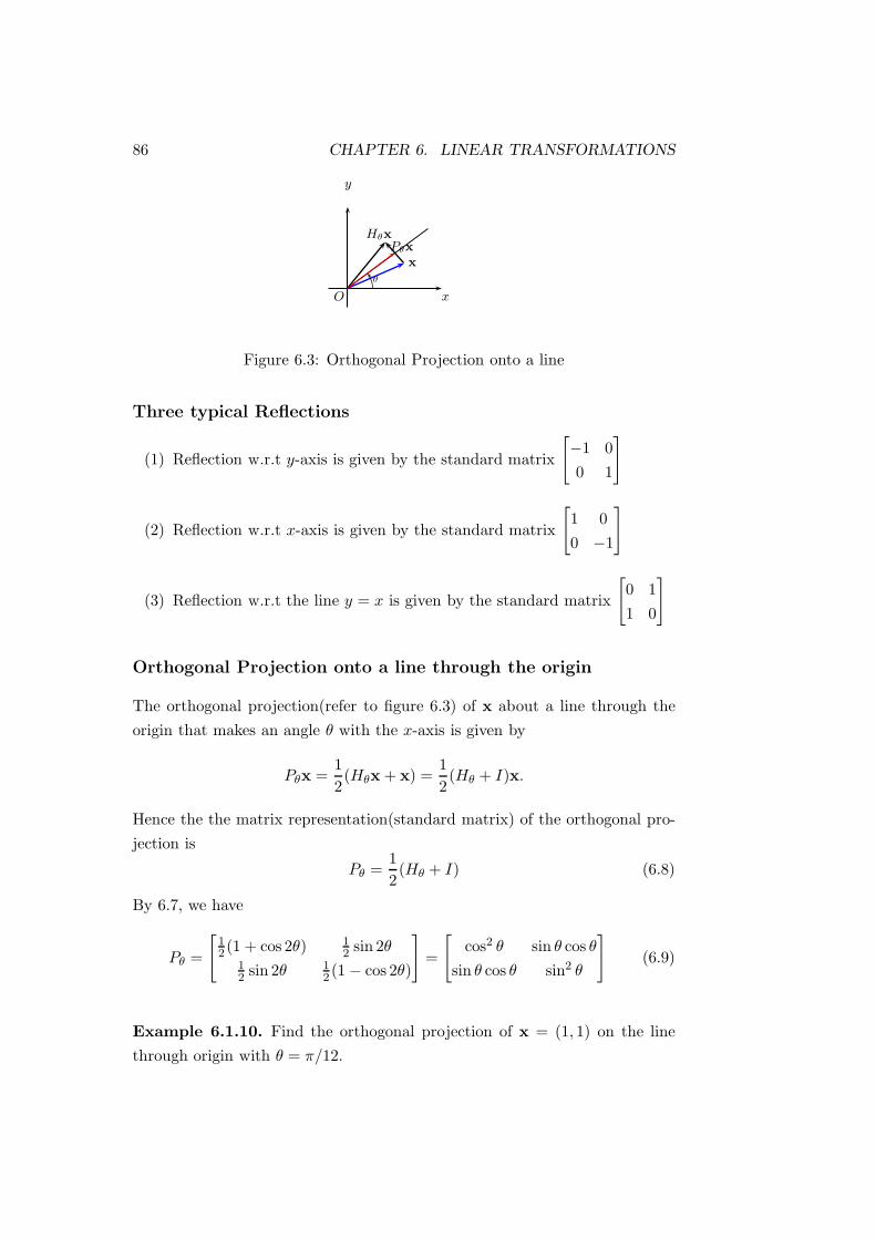
Figure 6.3: Orthogonal Projection onto a line
Three typical Reflections
(1) Reflection w.r.t y-axis is given by the standard matrix
[
−1 0
0 1
]
(2) Reflection w.r.t x-axis is given by the standard matrix
[
1 0
0 −1
]
(3) Reflection w.r.t the line y = x is given by the standard matrix
[
0 1
1 0
]
Orthogonal Projection onto a line through the origin
The orthogonal projection(refer to figure 6.3) of x about a line through the
origin that makes an angle θ with the x-axis is given by
Pθx =1
2(Hθx+ x) =
1
2(Hθ + I)x.
Hence the the matrix representation(standard matrix) of the orthogonal pro-
jection is
Pθ =1
2(Hθ + I) (6.8)
By 6.7, we have
Pθ =
[
12 (1 + cos 2θ) 1
2 sin 2θ12 sin 2θ
12 (1− cos 2θ)
]
=
[
cos2 θ sin θ cos θ
sin θ cos θ sin2 θ
]
(6.9)
Example 6.1.10. Find the orthogonal projection of x = (1, 1) on the line
through origin with θ = π/12.
6.2. GEOMETRY OF LINEAR OPERATORS 87
sol.
Pπ/12x =
[
12(1 + cos π
6 )12 sin
π6
12 sin
π6
12(1− cos π
6 )
] [
1
1
]
=
[
12 (1 +
√
32 ) 1
414
12(1−
√
32 )
] [
1
1
]
.
Transformation of a unit square
Power Sequence
6.2 Geometry of Linear Operators
Norm Preserving Linear Operators
Consider the linear operators given by the following matrices
Rθ =
[
cos θ − sin θ
sin θ cos θ
]
, Hθ =
[
cos 2θ sin 2θ
sin 2θ − cos 2θ
]
, Pθ =
[
cos2 θ sin θ cos θ
sin θ cos θ sin2 θ
]
Among these, the rotation and reflection do not change the length of a vector
and the angle between two vectors.
We say these operators are length preserving and angle preserving.
Definition 6.2.1. A linear operator T : Rn → Rn with length preserving
property ‖T (x)‖ = ‖x‖ is called an orthogonal operator.
Theorem 6.2.2. If T : Rn → Rn is a linear operator, then the followings are
equivalent.
(1) ‖T (x)‖ = ‖x‖ for all x ∈ Rn.
(2) T (x) · T (y) = x · y for all x,y ∈ Rn.
Proof. (1) ⇒ (2). We observe the following identity (polarization identity):
x · y =1
4(‖x+ y‖2 − ‖x− y‖2) (6.10)
Hence

88 CHAPTER 6. LINEAR TRANSFORMATIONS
T (x) · T (y) =1
4(‖T (x) + T (y)‖2 − ‖T (x) − T (y)‖2)
=1
4(‖T (x+ y)‖2 − ‖T (x− y)‖2)
=1
4(‖x+ y‖2 − ‖x− y‖2)
= x · y.
(2) ⇒ (1). Put x = y in (2) to get (1).
Orthogonal Operators Preserve Angle and Orthogonality
Definition 6.2.3. A square matrix is said to be orthogonal if A−1 = AT .
If an orthogonal operator T is represented by the matrix A then
T (x) = Ax.
Since ‖T (x)‖ = ‖x‖ we see by above theorem
x · y = Ax ·Ay = xTATAy (6.11)
for all x and y. Thus it is easy to deduce ATA = I by putting x = ei,y =
ej, i, j = 1, 2, · · · , n. Thus we have
Theorem 6.2.4. A linear operator T : Rn → Rn is orthogonal if and only if
the standard matrix is orthogonal.
Example 6.2.5.
A =
1√
2− 1
√
31√
6
0 1√
32√
61√
21√
3− 1
√
6
is an orthogonal matrix.
If T : Rn → Rn is an orthogonal operator, then
θ = cos−1
(
T (x) · T (y)
‖T (x)‖‖T (y)‖
)
= cos−1
(
x · y
‖x‖‖y‖
)
. (6.12)
This implies orthogonal operator preserves angles.

6.2. GEOMETRY OF LINEAR OPERATORS 89
Theorem 6.2.6. (1) The transpose of an orthogonal matrix is orthogonal.
(2) The inverse of an orthogonal matrix is orthogonal.
(3) The product of two orthogonal matrices is orthogonal.
(4) If A is orthogonal, then det(A) = ±1.
Proof. (3)
(AB)−1 = B−1A−1 = BTAT = (AB)T . (6.13)
Theorem 6.2.7. If A is an m×n is matrix, then the followings are equivalent.
(1) ATA = I.
(2) ‖Ax‖ = ‖x‖ for all x ∈ Rn.
(3) Ax ·Ay = x · y for all x,y ∈ Rn.
(4) The column vectors of A are orthonormal.
(5) The row vectors of A are orthonormal if m = n.
Proof. (2) ⇒ (3) requires polarization identity which holds for m× n matrix
also.
All Orthogonal Linear Operators on R2 are Rotations and Re-
flections
Theorem 6.2.8. If T : R2 → R2 is an orthogonal linear operator, then the
matrix representation(standard matrix) for T is of the form
Rθ =
[
cos θ − sin θ
sin θ cos θ
]
or Hθ/2 =
[
cos θ sin θ
sin θ − cos θ
]
(6.14)
Thus T is either a rotation(det(T ) = 1) or a reflection(det(T ) = −1).
Proof. ....
Contractions and Dilations on R2
The operator T (x, y) = (kx, ky) is called a scaling. It is called a contraction
if 0 ≤ k < 1 and called a dilation if k > 1.

90 CHAPTER 6. LINEAR TRANSFORMATIONS
O x
y
(1, 0) k > 0 k < 0
Figure 6.4: Shears along x
O x
y
(1, 0) k > 0 k < 0
Figure 6.5: Shears along y
Vertical Expansion and Compression on R2
The operator T (x, y) = (kx, y) is called an expansion in the x-direction if
k > 1, ( compression if k < 1). Similarly, the operator T (x, y) = (x, ky) is
called an expansion in the y-direction if k > 1, ( compression if k < 1).
Example 6.2.9. Refer to Tables 6.2.1 and 6.2.2 in p. 286. The contraction(or
a dilation), the expansion(or compression) in the x-direction, and expansion(or
compression) in the y-direction are given by the following matrices respectively.
[
k 0
0 k
]
,
[
k 0
0 1
]
, and
[
1 0
0 k
]
.
Shears
The operator T (x, y) = (x + ky, y) is a shear in the x-direction while the
operator T (x, y) = (x, y + kx) is a shear in the y-direction. They are
represented by[
1 k
0 1
]
, and
[
1 0
k 1
]
respectively.

6.2. GEOMETRY OF LINEAR OPERATORS 91
Linear Operators on R3
Basically we study two kinds of operators.
(1) length preserving operators (orthogonal operators)
(2) length non-preserving operators(e.g., projections)
First, examples of length non-preserving operators are projections.
Projection onto xy-plane is given by T (x, y, z) = (x, y, 0). Thus the stan-
dard matrix is
A =
1 0 0
0 1 0
0 0 0
Projection onto other planes are given by similar form of matrices.
Now we study length preserving operators (orthogonal operators).
Theorem 6.2.10. If T : R3 → R3 is an orthogonal linear operator, then one
of the following holds.
(1) Rotations about line through the origin.
(2) Reflections about planes through the origin.
(3) A rotation about line through the origin followed by a reflection about
the plane through the origin that is perpendicular to the line.
In fact, a 3 × 3 orthogonal matrix A represents a rotation if det(A) = 1 and
represents a type 2 or type 3 operator if det(A) = −1.
Reflections about Coordinate Planes
Reflections about xy-plane, yz-plane and zx-plane are respectively given by
T (x, y, z) = (x, y,−z), T (x, y, z) = (−x, y, z) and T (x, y, z) = (x,−y, z).
Their standard matrices are
1 0 0
0 1 0
0 0 −1
,
−1 0 0
0 1 0
0 0 1
, and
1 0 0
0 −1 0
0 0 1

92 CHAPTER 6. LINEAR TRANSFORMATIONS
Rotations in R3
Consider the rotations in R3: The key point is to know the axis of rotation
and the orientation(direction of rotation). To find the axis of rotation, we
note that the vector along the axis is not changed under the rotation. Next
we consider how to choose direction of rotation. For example, we choose a
vector w in the plane and rotate it by T . Let
u = w × T (w)
Take the view point at the tip of the vector u(right handed rule). We call this
u an orientation of the rotation.
w × T (w)
θ
T (w)
w
W
Figure 6.6: Oriented axis of rotation
x
y
z
b
θ
Figure 6.7: The rotation about x-axis by θ
Two questions
There are two questions regarding the rotations in R3.

6.2. GEOMETRY OF LINEAR OPERATORS 93
(1) Given a rotation, how to find the standard matrix representing the ro-
tation?
(2) Given a standard rotation matrix A, how to find the axis and angle of
rotation ?
To answer the first question, consider, for example, the rotation about x-
axis by θ. Under the given rotation, the vector e1 is fixed, while e2 and e3 are
mapped to (0, cos θ, sin θ) and (0,− sin θ, cos θ), resp. i.e.,
e1Rx,θ⇒
1
0
0
, e2
Rx,θ⇒
0
cos θ
sin θ
, e3
Rx,θ⇒
0
− sin θ
cos θ
Thus the rotation about x-axis by θ is given by the standard matrix
Rx,θ =
1 0 0
0 cos θ − sin θ
0 sin θ cos θ
To answer the second question, note that the axis remains fixed under the
matrix A, we have
(I −A)x = 0
Once we know the axis, choose a nonzero vector w perpendicular to the
axis and compute Aw. Finally, we obtain the angle of rotation by the formula:
cos θ =w ·Aw
‖w‖ ‖Aw‖. (6.15)
Example 6.2.11. (1) Show the matrix represents a rotation about a line
through the origin.
A =
1 0 0
0 0 −1
0 1 0
(2) Find the axis and angle of the rotation given by the matrix

94 CHAPTER 6. LINEAR TRANSFORMATIONS
(3) Repeat the question with
A =
0 1 0
1 0 0
0 0 −1
sol. (1) Since A is orthogonal and det(A) = 1, it is a rotation. To find the
axis of rotation, solve (I −A)x = 0, i.e.,
0 0 0
0 1 1
0 −1 1
x
y
z
=
0
0
0
⇒
x
y
z
=
1
0
0
Thus it is the rotation in yz-plane.
(2) To find the angle, choose any vector, say w = (0, 1, 0) in the yz-plane
and compute Aw = (0, 0, 1). Thus
cos θ =w ·Aw
‖w‖ ‖Aw‖= 0 (6.16)
and hence θ = π/2.
(3) (I − A)x = 0 gives x = (1, 1, 0). The plane of rotation is a plane
perpendicular to (1, 1, 0). i.e., vectors lying in the plane satisfies
x+ y = 0.
Hence we choose a vector as w = (1,−1, 0) and we see Aw = (−1, 1, 0). Hence
the angle is
θ = cos−1 w ·Aw
‖w‖ ‖Aw‖= cos−1
(
−2
2
)
= π. (6.17)
There is a formula: From Theorem 6.2.8 of the book, we have
tr(A) = (a2 + b2 + c2)(1 − cos θ) + 3 cos θ = 1 + 2 cos θ
from which we have
cos θ =tr(A)− 1
2. (6.18)

6.3. KERNEL AND RANGE OF A TRANSFORMATION 95
6.3 Kernel and Range of a Transformation
Kernel
Let T is a linear operator on Rn and v ∈ R
n. Let x = tv be a line through
the origin. Then
T (x) = T (tv) = tT (v).
We will investigate the geometry of the image. There are two possibilities:
(1) If T (v) = 0 then T (x) = 0 for all x ∈ Rn. So the image is the one point
0.
(2) If T (v) 6= 0 then the image T (x) is a line through the origin.
Similarly, if x = t1v1 + t2v2 is a plane through the origin, then the image
under T is the set
T (x) = t1T (v1) + t2T (v2)
Hence there are three possibilities:
(1) If T (v1) = 0 and T (v2) = 0, then T (x) = 0 for all x ∈ Rn. So the image
is the one point 0.
(2) If T (v1) 6= 0 and T (v2) 6= 0, then the image T (x) is a plane through the
origin.
(3) In the other cases, the image T (x) is the line through the origin.
Definition 6.3.1. If T is a linear operator Rn → R
m, then the set of all
vectors in Rn that are mapped to 0 by T is called kernel of T and denoted
by ker(T ).
Example 6.3.2. Find the kernel of the following linear operators in R3.
(1) The zero operator T0(x) = 0x = 0.
(2) The identity operator I(x) = Ix = x.
(3) The orthogonal projection on the xy-plane.
(4) A rotation about the line through the origin with angle θ.
Theorem 6.3.3. If T : Rn → R
m is a linear transformation, then the kernel
of T is a subspace of Rn.

96 CHAPTER 6. LINEAR TRANSFORMATIONS
Kernel of a Matrix Transformation
Theorem 6.3.4. The kernel of an m × n matrix transformation A is the
solution of Ax = 0.
Definition 6.3.5. If A is m× n matrix, then the solution space of the linear
system Ax = 0 (or, equivalently, the kernel of TA) is called the null space of
A and denoted by null(A).
Example 6.3.6. Find the null space of the following matrix.
A =
1 3 −2 0 2 0
2 6 −5 −2 4 −3
0 0 5 10 0 15
2 6 0 8 4 18
Reducing to row echelon form by Gaussian(Jordan) elimination, we obtain
1 3 0 4 2 0
0 0 1 2 0 0
0 0 0 0 0 1
0 0 0 0 0 0
Hence we get
x1 +3x2 +4x4 +2x5 = 0
x3 +2x4 = 0
x6 = 0
(6.19)
Solving
x1 = −3x2 − 4x4 − 2x5
x2 = −2x4
x6 = 0
(6.20)
Thus we have
x1 = −3r − 4s− 2t, x2 = r, x3 = −2s, x4 = s, x5 = t, x6 = 0
and we find the solutions of Ax = 0 are linear combinations of the following
vectors
[−3, 1, 0, 0, 0, 0], [−4, 0,−2, 1, 0, 0], [−2, 0, 0, 0, 1, 0].
Theorem 6.3.7. If T : Rn → R
m is a linear transformation, then T maps

6.3. KERNEL AND RANGE OF A TRANSFORMATION 97
subspaces of Rn into subspaces of Rm.
Range of a Linear Transformation
Definition 6.3.8. If T : Rn → Rm is a linear transformation, then the set of
all vectors in Rm that consist of all the images of T is called the range of T
and denoted by ran(T ).
Example 6.3.9. Find the range of the following linear operators in R3.
(1) The zero operator T0(x) = 0x = 0.
(2) The identity operator I(x) = Ix = x.
(3) The orthogonal projection on the xy-plane.
(4) A rotation about the line through the origin with angle θ.
Theorem 6.3.10. If T : Rn → R
m is a linear transformation, then ran(T )
is a subspace of Rm.
Range of a Matrix Transformation
Theorem 6.3.11. If A is an m×n matrix, then the range of the corresponding
linear transformation is the column space of A.
Example 6.3.12. Determine whether the vector b is in the range(column
space) of A when A and b are given as follows.
A =
1 −8 −7 −4
2 −3 −1 5
3 2 5 14
, and b =
8
−10
−28
sol. Reduce the augmented matrix to the echelon form:
1 0 1 4 −8
0 1 1 1 −2
0 0 0 0 0
From this we get
x1 = −8− s− 4t, x2 = −2− s− t, x3 = s, x4 = t.

98 CHAPTER 6. LINEAR TRANSFORMATIONS
Thus there is at least one solution which is
x1 = −8, x2 = −2, x3 = x4 = 0.
Thus b is in the range of A.
Existence and Uniqueness
Given a linear transformation T : Rn → Rm we have the following question:
(1) The existence question- Is every vector in Rm the image of at least one
vector in Rn ?
(2) Can two distinct vectors in Rn have the same image in R
m ?
Definition 6.3.13. A linear transformation T : Rn → Rm is said to be onto
if its range is entire codomain Rm; that is every vector in R
m is the image of
at least one vector in Rn.
Definition 6.3.14. A linear transformation T : Rn → Rm is said to be one-
to-one if T maps distinct vectors in Rn into distinct vectors in R
m.
Theorem 6.3.15. If T : Rn → R
m is a linear transformation, then the
following statements are equivalent:
(1) T is one-to-one.
(2) ker(T ) = 0.
One-to-one and Onto from the Viewpoint of Linear System
Theorem 6.3.16. If A is an m × n matrix, then the corresponding linear
transformation TA is one-to-one if and only if the linear system Ax = 0 has
trivial solution.
Theorem 6.3.17. If A is an m × n matrix, then the corresponding linear
transformation TA is onto if and only if the linear system Ax = b is consistent
for every b ∈ Rm.
Theorem 6.3.18. If A is an n × n matrix, then the corresponding linear
transformation TA is one-to-one if and only if it is onto.

6.4. COMPOSITIONAND INVERTIBILITY OF LINEAR TRANSFORMATIONS99
A Unifying Theorem- Theorem 6.3.15
Theorem 6.3.19. (1) Reduced echelon form is In.
(2) A is expressible as a product of elementary matrices.
(3) A is invertible.
(4) Ax = 0 has only trivial solution.
(5) Ax = b is consistent for any b ∈ Rn.
(6) Ax = b has exactly one solution for any b ∈ Rn.
(7) The column vectors are linearly independent.
(8) The row vectors are linearly independent.
(9) det(A) 6= 0.
(10) λ = 0 is not an eigenvalue of A.
(11) TA is one-to-one.
(12) TA is onto.
6.4 Composition and Invertibility of Linear Trans-
formations
Composition of Linear Transformations
If T1 : Rn → Rk and T2 : Rk → R
m are two linear transformations, then we
can consider their composition, called composition of T2 with T1.
(T2 ◦ T1)(x) = T2(T1(x)) (6.21)
Theorem 6.4.1. If T1 : Rn → R
k and T2 : Rk → R
m are two linear transfor-
mations, then (T2 ◦ T1) : Rn → R
m is also a linear transformation.
Theorem 6.4.2. If A : k×n and B : n×m are two linear matrices, then the
m× n matrix BA is the standard matrix of the corresponding composition of
linear transformations.

100 CHAPTER 6. LINEAR TRANSFORMATIONS
Example 6.4.3. Consider composition of two rotation transformations:
Rx,θ1 =
[
cos θ1 − sin θ1
sin θ1 cos θ1
]
and Rx,θ2 =
[
cos θ2 − sin θ2
sin θ2 cos θ2
]
(6.22)
Rx,θ2Rx,θ1 =
[
cos θ2 − sin θ2
sin θ2 cos θ2
] [
cos θ1 − sin θ1
sin θ1 cos θ1
]
=
[
cos θ3 − sin θ3
sin θ3 cos θ3
]
(6.23)
where θ3 = θ1 + θ2.
Thus Rx,θ2Rx,θ1 = Rx,θ1+θ2 .
Example 6.4.4. Consider composition of two reflections:
Hθ1 =
[
cos 2θ1 sin 2θ1
sin 2θ1 − cos 2θ1
]
and Hθ2 =
[
cos 2θ2 sin 2θ2
sin 2θ2 − cos 2θ2
]
. (6.24)
Hθ2Hθ1 =
[
cos 2θ2 sin 2θ2
sin 2θ2 − cos 2θ2
][
cos 2θ1 sin 2θ1
sin 2θ1 − cos 2θ1
]
=
[
cos 2(θ2 − θ1) − sin 2(θ2 − θ1)
sin 2(θ2 − θ1) cos 2(θ2 − θ1)
]
Thus the composition of two reflections is a rotation:
Hθ2Hθ1 = R2(θ2−θ1)
This can be expected from the fact that the determinant of product of the
corresponding matrices is det(Hθ2Hθ1) = det(Hθ2)det(Hθ1) = (−1)(−1) = 1.
Example 6.4.5 (Composition is not a commutative operation). Consider the
composition of two matrices:
A1 =
[
1 2
0 1
]
and A2 =
[
0 1
1 0
]
. (6.25)
We see
A2A1 =
[
0 1
1 2
]
, while A1A2 =
[
2 1
1 0
]

6.4. COMPOSITIONAND INVERTIBILITY OF LINEAR TRANSFORMATIONS101
Composition of Three Transformations
If
T1 : Rn → R
k , T2 : Rk → R
ℓ and T3 : Rℓ → R
m
are three linear transformations, then we define their composition Rn → R
m
by
(T3 ◦ T2 ◦ T1)(x) = T3(T2(T1(x))) (6.26)
Factoring of a Linear Operators
Example 6.4.6. Consider
D =
[
λ1 0
0 λ2
]
=
[
1 0
0 λ2
][
λ1 0
0 1
]
= D1D2. (6.27)
Theorem 6.4.7. If A is an invertible 2 × 2 matrix, then the corresponding
linear operator is a composition of shears, compression, and expansions in the
direction of coordinate axes, and the reflection about the coordinate axes and
about the line y = x.
Example 6.4.8. Express the following as a composition of operator with
geometric meaning.
A =
[
1 2
3 4
]
Use elementary row operations:
[
1 2
0 −2
]
E21(−3)→
[
1 2
0 1
]
R2(−12)
→
[
1 2
0 1
]
(6.28)
So[
1 0
0 −12
] [
1 0
−3 1
]
A =
[
1 2
0 1
]
we have
A =
[
1 0
3 1
][
1 0
0 −2
] [
1 2
0 1
]
Inverse of a Linear Transformation
If T : Rn → Rm is a one-to-one linear transformation, then each vector w
in the range of T is the image of a unique vector x in Rn. We call it the

102 CHAPTER 6. LINEAR TRANSFORMATIONS
preimage of w. In this case we can define the inverse of T by
T−1(w) = x if and only if T (x) = w
Theorem 6.4.9. If T : Rn → R
n is a one-to-one linear operator, and if A is
the standard matrix of T , then A is invertible and A−1 is the standard matrix
of T−1.
Image of the Unit Square under a Linear Transformation
Example 6.4.10. Find the image of the unit square under the following linear
operators.
A[T (e1) T (e2)] =
[
x1 x2
y1 y2
]
.
Theorem 6.4.11. If T : R2 → R
2 is an invertible linear operator, then
the area of the parallelogram formed by T (e1) and T (e2) is det (A), where
A =[
T (e1) T (e2)]
.