line and curve fitting - york university€¦ · leverage points in line fitting in line fitting, a...
TRANSCRIPT

Line and curve fitting
1

Line fitting in MATLAB MATLAB provides a function for performing least-
squares polynomial fitting a line is a polynomial of degree 1
>> x = [-4; 3.7; 0; 2.5; 1.2; -2.8; -1.4];
>> y = [-37; 38; 0; 29; 21; -21; -8];
>> polyfit(x, y, 1)
ans =
9.7436 4.2564
this says that the best fit line is 𝑦 = 9.7436𝑥 + 4.2564
2

Line fitting in MATLAB MATLAB provides a function named polyval for
evaluating the polynomial computed by polyfit
>> coeffs = polyfit(x, y, 1);
>> yfit = polyval(coeffs, x)
yfit =
-34.7182
40.3079
4.2564
28.6155
15.9488
-23.0258
-9.3847
3
the best fit line 𝑦 = 𝑎 + 𝑏𝑥 evaluated at each value in x

Line fitting in MATLAB computing the residual errors is easy using polyval
>> coeffs = polyfit(x, y, 1);
>> yfit = polyval(coeffs, x);
>> res = y - yfit
res =
-2.2818
-2.3079
-4.2564
0.3845
5.0512
2.0258
1.3847
4
the residual errors 𝑟𝑖 = 𝑦𝑖 − (𝑎 + 𝑏𝑥𝑖)
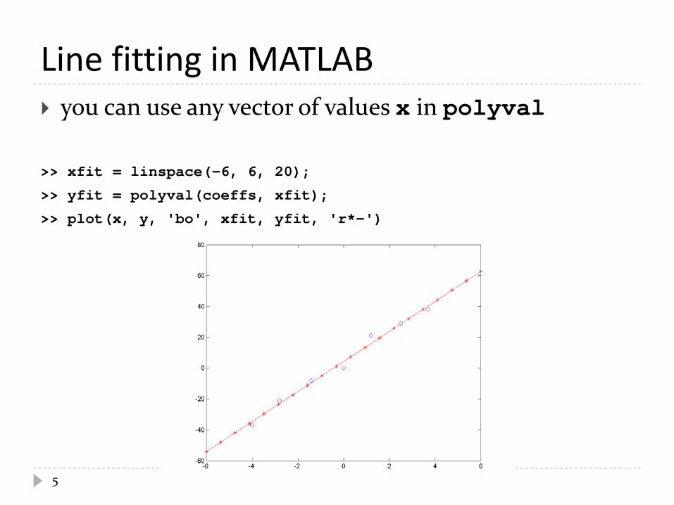
Line fitting in MATLAB you can use any vector of values x in polyval
>> xfit = linspace(-6, 6, 20);
>> yfit = polyval(coeffs, xfit);
>> plot(x, y, 'bo', xfit, yfit, 'r*-')
5

Leverage points in line fitting in line fitting, a high leverage point is a measurement
made near the extremes of the range of independent variable if this measurement is erroneous, or can only be made with
low precision, then it will have a large effect on the fitted line
6

Leverage points in line fitting effect of a high leverage point on a line fit
7

Leverage points in line fitting effect of a low leverage point on a line fit
8

Transforming non-linear relationships line fitting can be applied to a non-linear problem if
the problem can be transformed into a linear one; e.g., Newton's law of cooling states that the rate of change
of the temperature of an object is proportional to the difference between the temperature of the object and its surrounding environment it can be shown that the temperature of the object as a
function of time is: where 𝑇0 is the temperature at 𝑡 = 0, 𝑇𝑒𝑒𝑒 is the temperature of the surrounding environment, and 𝑟 is a constant
9
𝑇 𝑡 = 𝑇𝑒𝑒𝑒 + (𝑇0 − 𝑇𝑒𝑒𝑒)𝑒−𝑟𝑟
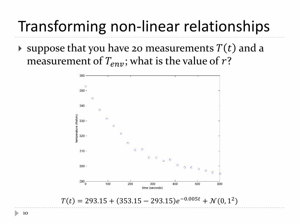
Transforming non-linear relationships suppose that you have 20 measurements 𝑇 𝑡 and a
measurement of 𝑇𝑒𝑒𝑒; what is the value of 𝑟?
10
𝑇 𝑡 = 293.15 + 353.15 − 293.15 𝑒−0.005𝑟 + 𝒩(0, 12)

Transforming non-linear relationships to use line fitting, we need a linear relationship in 𝑡 in this case, a straightforward transformation exists:
11
𝑇 𝑡 = 𝑇𝑒𝑒𝑒 + 𝑇0 − 𝑇𝑒𝑒𝑒 𝑒−𝑟𝑟
𝑇 − 𝑇𝑒𝑒𝑒𝑇0 − 𝑇𝑒𝑒𝑒
= 𝑒−𝑟𝑟
ln𝑇 − 𝑇𝑒𝑒𝑒𝑇0 − 𝑇𝑒𝑒𝑒
= −𝑟𝑡

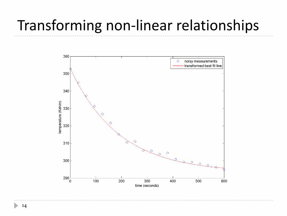
Transforming non-linear relationships % t time vector
% T temperature measurements taken at t
% T0 353.15 K
% Tenv 293.15 K
U = log((T - Tenv) / (T0 - Tenv));
coeffs = polyfit(t, U, 1);
Ufit = polyval(coeffs, t);
plot(t, U, 'o', t, Ufit, 'r-');
slope = coeffs(1); % what is coeffs(2)?
r = -slope % should be 0.005
12

Transforming non-linear relationships
13
Transforming non-linear relationships
14
Transforming non-linear relationships exercise for the student: you have to be very careful when using this approach; why? hint
extend the measurements 𝑇(𝑡) to 𝑡 = 1200 𝑠 and perform the same analysis
can you explain the appearance of the plot of U = log((T - Tenv) / (T0 - Tenv))when you extend the measurements to 𝑡 = 1200 𝑠?
15

Polynomial fitting in MATLAB polyfit can be used to fit a polynomial of any degree
suppose that at time 𝑡 = 0 𝑠 you launch a ball straight
up with an unknown initial velocity and unknown initial height
starting at time 𝑡 = 1 𝑠, you obtain measurements of the height 𝑦(𝑡) of the ball
find the initial velocity and initial height of the ball
16

Polynomial fitting in MATLAB
17
𝑦 𝑡 = −12𝑔𝑡
2 + 15𝑡 + 2 + 𝒩(0, 0.052) 𝑣0 = 15 𝑚𝑠 , 𝑦0 = 2 𝑚
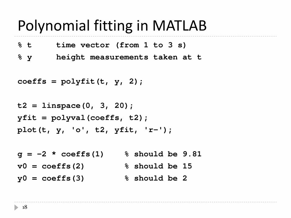
Polynomial fitting in MATLAB % t time vector (from 1 to 3 s)
% y height measurements taken at t
coeffs = polyfit(t, y, 2);
t2 = linspace(0, 3, 20);
yfit = polyval(coeffs, t2);
plot(t, y, 'o', t2, yfit, 'r-');
g = -2 * coeffs(1) % should be 9.81
v0 = coeffs(2) % should be 15
y0 = coeffs(3) % should be 2
18

Polynomial fitting in MATLAB
19
𝑣0� = 15.3073 𝑚𝑠 ,
𝑦0� = 1.7568 𝑚
𝑔� = 9.9842 𝑚𝑠2
values from fitting
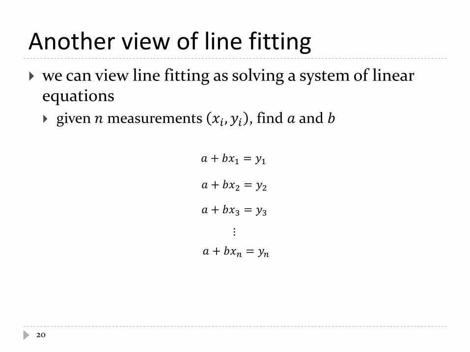
Another view of line fitting we can view line fitting as solving a system of linear
equations given 𝑛 measurements 𝑥𝑖 ,𝑦𝑖 , find 𝑎 and 𝑏
20
𝑎 + 𝑏𝑥1 = 𝑦1
𝑎 + 𝑏𝑥2 = 𝑦2
𝑎 + 𝑏𝑥3 = 𝑦3
𝑎 + 𝑏𝑥𝑒 = 𝑦𝑒 ⋮

Another view of line fitting in matrix form:
which can be solved in MATLAB in a least-squares sense as 𝐱 = 𝐀 ∖ 𝐲
21
𝑎 + 𝑏𝑥1 = 𝑦1
𝑎 + 𝑏𝑥2 = 𝑦2
𝑎 + 𝑏𝑥3 = 𝑦3
𝑎 + 𝑏𝑥𝑒 = 𝑦𝑒 ⋮
1 𝑥11 𝑥21 𝑥3⋮
1 𝑥𝑒
𝑎𝑏 =
𝑦1𝑦2𝑦3⋮𝑦𝑒
𝐀 𝐱 𝐲
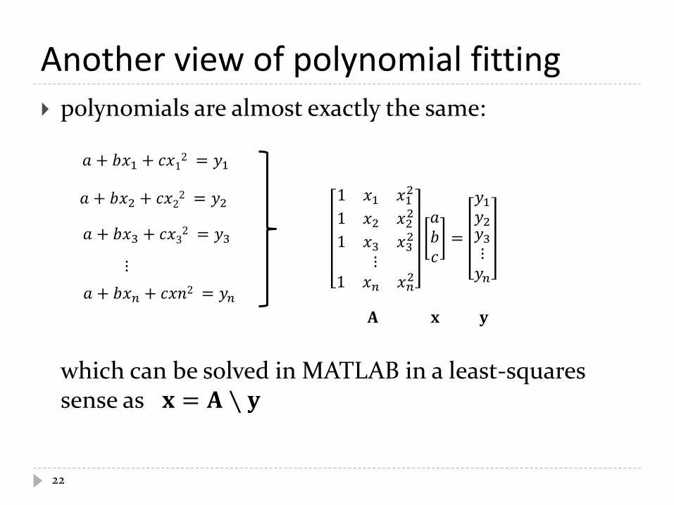
Another view of polynomial fitting polynomials are almost exactly the same:
which can be solved in MATLAB in a least-squares sense as 𝐱 = 𝐀 ∖ 𝐲
22
𝑎 + 𝑏𝑥1 + 𝑐𝑥12 = 𝑦1
𝑎 + 𝑏𝑥2 + 𝑐𝑥22 = 𝑦2
𝑎 + 𝑏𝑥3 + 𝑐𝑥32 = 𝑦3
𝑎 + 𝑏𝑥𝑒 + 𝑐𝑥𝑛2 = 𝑦𝑒 ⋮
1 𝑥1 𝑥12
1 𝑥2 𝑥22
1 𝑥3 𝑥32⋮
1 𝑥𝑒 𝑥𝑒2
𝑎𝑏𝑐
=
𝑦1𝑦2𝑦3⋮𝑦𝑒
𝐀 𝐱 𝐲

Another view of polynomial fitting a matrix 𝐀 of the form
is called a Vandermonde matrix
23
1 𝑥1 𝑥12 … 𝑥1𝑚
1 𝑥2 𝑥22 … 𝑥2𝑚
1 𝑥3 𝑥32 … 𝑥3𝑚⋮
1 𝑥𝑒 𝑥𝑒2 … 𝑥𝑒𝑚