Line Graph Analysis using R Script for Intel Edison - IoT Foundation data

Neeraja Ganesan | nganesa@us.ibm.com | @neerajaganesan

Part 1: Sending internal temp. sensor data from Intel Edison to IBM IoT Platform 1. After setting the Edison up, using serial port or Wifi, log into it on command prompt/terminal.Note down INET address of Edison. Eg: Mine is 192.168.1.9, after you connect your device, it will be something else.

2. Download a File transfer client, e.g.: Filezilla

3. Go to your pendrive 4. Look for folder BluemixFiles 5. Inside that download ibm-iot-quickstart on your machine OR go to : https://developer.ibm.com/recipes/tutorials/connect-an-intel-galileo-to-the-internet-of-things-foundation-connect/ and download ibm-iot-quickstart.zip from step 3. a). 6. Go back to FileZilla dialog and SSH into it. Note that the Edison needs to have a username and password in order for a FileZilla connection to be established. Configure the setup if necessary.

7. Drag and drop ibm-iot-quickstart from the unzipped download on the left pane into the root folder of Edison on the right pane.

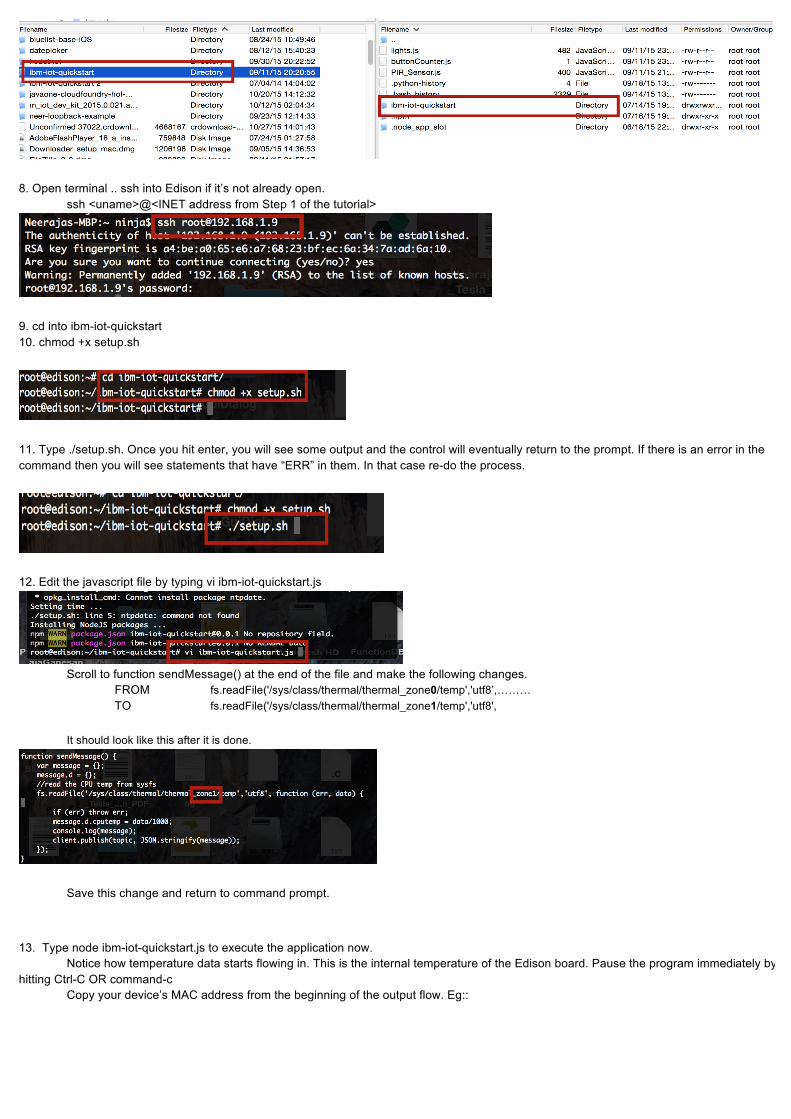
8. Open terminal .. ssh into Edison if it’s not already open. ssh <uname>@<INET address from Step 1 of the tutorial>

9. cd into ibm-iot-quickstart 10. chmod +x setup.sh

11. Type ./setup.sh. Once you hit enter, you will see some output and the control will eventually return to the prompt. If there is an error in the command then you will see statements that have “ERR” in them. In that case re-do the process.

12. Edit the javascript file by typing vi ibm-iot-quickstart.js

Scroll to function sendMessage() at the end of the file and make the following changes. FROM fs.readFile('/sys/class/thermal/thermal_zone0/temp','utf8’,……… TO fs.readFile('/sys/class/thermal/thermal_zone1/temp','utf8', It should look like this after it is done.

Save this change and return to command prompt. 13. Type node ibm-iot-quickstart.js to execute the application now. Notice how temperature data starts flowing in. This is the internal temperature of the Edison board. Pause the program immediately by hitting Ctrl-C OR command-c Copy your device’s MAC address from the beginning of the output flow. Eg::

14. Open the following link https://quickstart.internetofthings.ibmcloud.com/#/ and paste the MAC address from the previous step into the QuickStart text box and Click “Go” 15. Keeping this tab open, open the terminal/command prompt now and type node ibm-iot-quickstart.js again and notice how the graph starts showing real time temperature data in the browser URL

Continue to the next page for Part 2…...

Part 2: Connecting a Grove Temperature Sensor, and fetching data from there, and sending it to Bluemix Cloud ******Connect a temperature sensor to the Edison board at Analog Pin 0, after placing the Base Shield on top of the Edison

16. Open Intel Edison on Terminal/Command Prompt and cd into folder ibm-iot-quickstart, then vi ibm-iot-quickstart.js Add the following lines on top, before var mqtt is declared: var groveSensor = require(‘jsupm_grove’); var temp = new groveSensor.GroveTemp(0);

17. Scroll down to the end of the file and add the following lines of code to display outside temperature: var celsius = temp.value(); message.d.outsidetemp = celsius; BEFORE the statement console.log(message); NOTE : The statement should now look like this after making the change, add the line “var celsius = temp.value();” before setting message.d.outsidetemp = celsius:

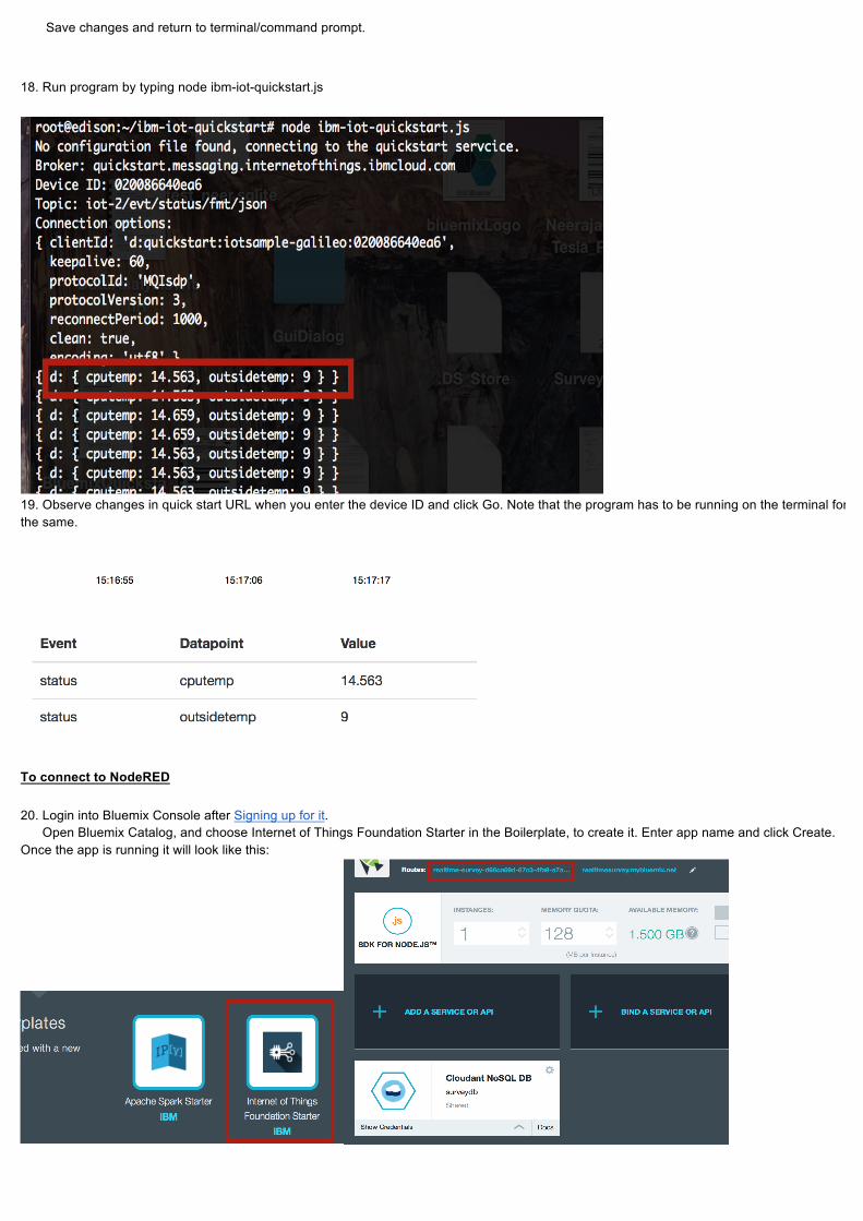
Save changes and return to terminal/command prompt. 18. Run program by typing node ibm-iot-quickstart.js

19. Observe changes in quick start URL when you enter the device ID and click Go. Note that the program has to be running on the terminal for the same.

To connect to NodeRED 20. Login into Bluemix Console after Signing up for it. Open Bluemix Catalog, and choose Internet of Things Foundation Starter in the Boilerplate, to create it. Enter app name and click Create. Once the app is running it will look like this:

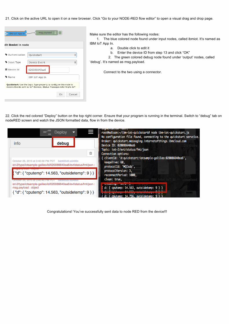
21. Click on the active URL to open it on a new browser. Click “Go to your NODE-RED flow editor” to open a visual drag and drop page.

Make sure the editor has the following nodes:

1. The blue colored node found under input nodes, called ibmiot. It’s named as IBM IoT App In.

a. Double click to edit it b. Enter the device ID from step 13 and click “OK”

2. The green colored debug node found under ‘output’ nodes, called ‘debug’. It’s named as msg.payload.

Connect to the two using a connector.

22. Click the red colored “Deploy” button on the top right corner. Ensure that your program is running in the terminal. Switch to “debug” tab on nodeRED screen and watch the JSON formatted data, flow in from the device.

Congratulations! You’ve successfully sent data to node RED from the device!!!

Part 3: Creating table in the data base 23. Switch to a new tab and open the app overview page in the Bluemix dashboard page and click “Add a service”.

24. From the catalog page that opens, click dashDB service from Database Management.

25. Enter a name for the service and click “Create”. 26. When prompted to “Restage” the application, click “Ok”. 27. Once the application starts running again, click DashDB service from app overview and click “Launch”.

28. From the left pane click “Tables” and when that opens, click “Add Table”

29. Create a table using SQL statements. Eg: table name is IBM_BLUEMIX: CREATE TABLE “IBM_BLUEMIX” ( “TIME” VARCHAR(20), “TEMP” VARCHAR(5) );

30. Once the DDL runs successfully, it can be verified by viewing that that table name shows up, in the drop down that shows for existing tables, under the schema. An auto generated schema is created if no schema is chosen.

If the refresh button near the table name is clicked, column names show up below table name. Now we populate table with data 31. Go back to the tab that has the nodeRED editor open. It can be opened by clicking the URL on the app overview page and then clicking the button that says “Go to your Node-RED flow editor”. 32. Drag the “function” node from the left pane and connect it to the Blue colored “IBM IoT App In” node. 33. Double click the function node to open it. Now we’re adding data to extract it from the device. Since we’re expecting to send this data to the database, we will enter following data in the editor as shown in the image. If desired, name the node at the Name text area. Here it has been named “FormatDataForDB”

34. Drag the dashDB output node from the pane on the left and connect it to this function, such that the function serves as an input to the database. dashDB can be found under “storage” heading. Choose the node that has a connector option only to the left(i.e. last node under the heading). Establish a connector between the newly created function node and dashDB node. 35. Double click the dashDB node, enter the table name, as created in step 7. Under the service drop down, click the name of the dashDB service as it is named in the app overview page. Remember to bind the service if it you don’t see it.

36. Click “Deploy” to incorporate these changes. Ensure that no error is seen on the Debug tab. If an error is seen then verify the dashDB connection or javascript syntax.

37. With the program running on the terminal, verify that data is sent to dashDB by launching the service from the dashboard page. Click “Tables” on the left pane -> Choose appropriate <SCHEMA_NAME> and “<TABLE NAME>” from existing tables -> Click “Browse Data” tab. When data is loaded, we can be sure of nodeRED sending data to the back end. Note that TEMP column that you see under heading outsidetemp in nodeRED and terminal. We are recording system time and storing it for a comprehensive graph.

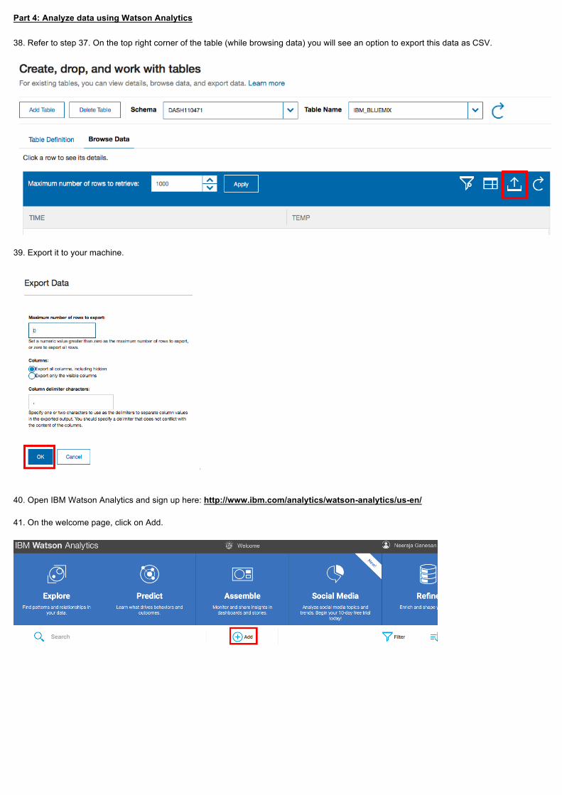
Part 4: Analyze data using Watson Analytics 38. Refer to step 37. On the top right corner of the table (while browsing data) you will see an option to export this data as CSV.

39. Export it to your machine.

40. Open IBM Watson Analytics and sign up here: http://www.ibm.com/analytics/watson-analytics/us-en/ 41. On the welcome page, click on Add.

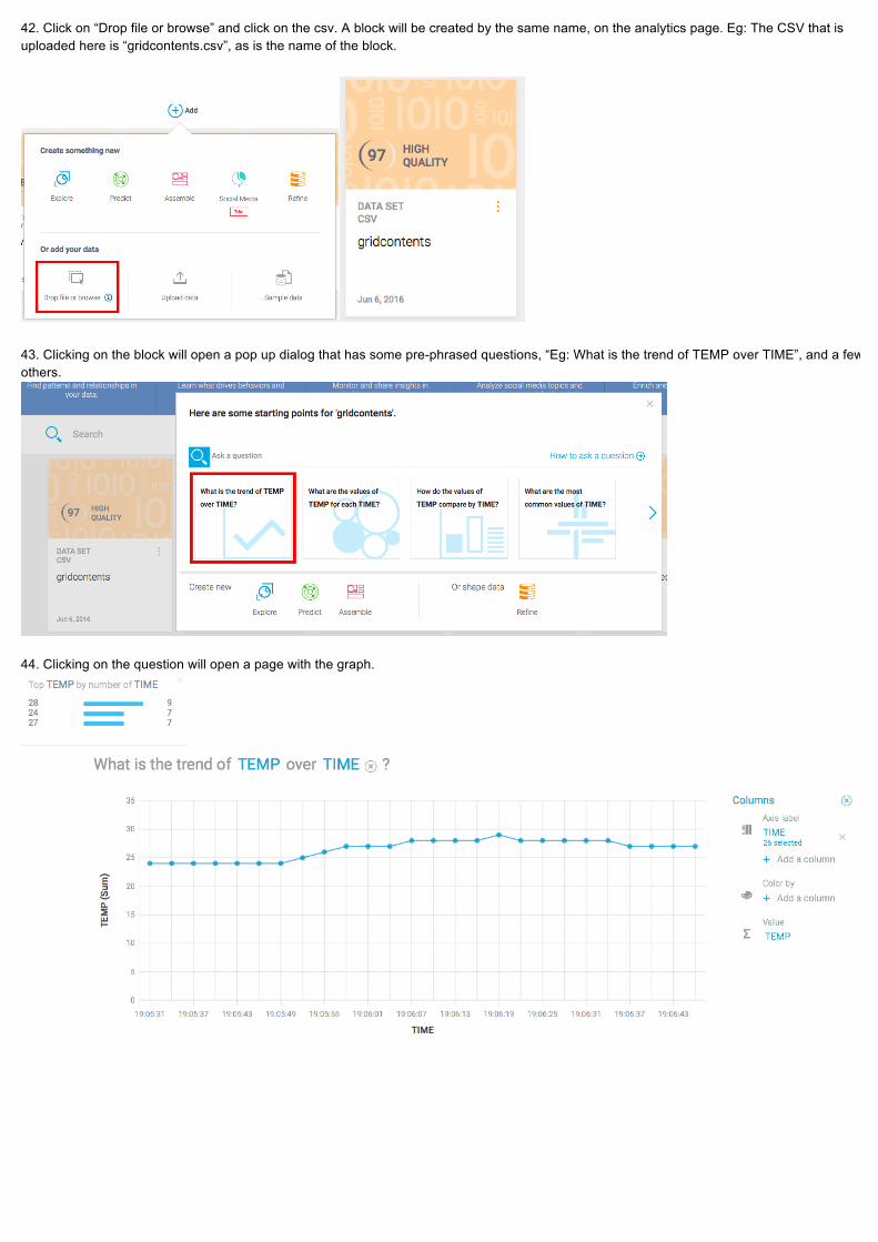
42. Click on “Drop file or browse” and click on the csv. A block will be created by the same name, on the analytics page. Eg: The CSV that is uploaded here is “gridcontents.csv”, as is the name of the block.

43. Clicking on the block will open a pop up dialog that has some pre-phrased questions, “Eg: What is the trend of TEMP over TIME”, and a few others.

44. Clicking on the question will open a page with the graph.

Part 5: Analyze data using Apache Spark 45. Open app on App overview page and click on “Add a service or API”.

46. When the catalog page opens, scroll down to “Data and Analytics” and click on “Apache Spark”. Enter name for the service and let the plan remain “Personal” by default. Click on Create. NOTE: Both “Space” and “App” are greyed out. These parameters are fixed since the service is now being bound to this app.

47. Click on the “Restage” button when prompted. The application will now restart with the new service as part of it.

48. On the App Overview page, click on the “Apache Spark” instance that you just created and then click on Notebook.

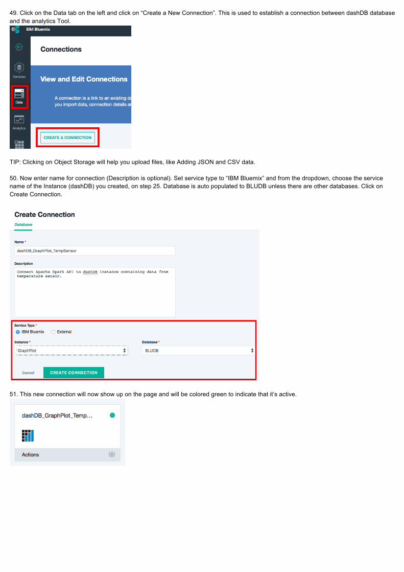
49. Click on the Data tab on the left and click on “Create a New Connection”. This is used to establish a connection between dashDB database and the analytics Tool.

TIP: Clicking on Object Storage will help you upload files, like Adding JSON and CSV data. 50. Now enter name for connection (Description is optional). Set service type to “IBM Bluemix” and from the dropdown, choose the service name of the Instance (dashDB) you created, on step 25. Database is auto populated to BLUDB unless there are other databases. Click on Create Connection.

51. This new connection will now show up on the page and will be colored green to indicate that it’s active.

52. On the left, pane click on “Analytics” tab.

53. Click on “New Notebook” to create a new notebook into which you’ll be adding Python code. 54. Enter name and description for notebook and click “Create Notebook”. The overview page will now show the newly created notebook.

55. This will now open to a empty workbook with “Python 2.0” as version number on the top right corner

NOTE: In the following step, click run button after typing code in each cell, to execute code. Code is available in pen drive (“temp_analysis_python.txt”)

Refer to step 56 to see how code is supposed to look

56. Type the following code into your python notebook, cell by cell.

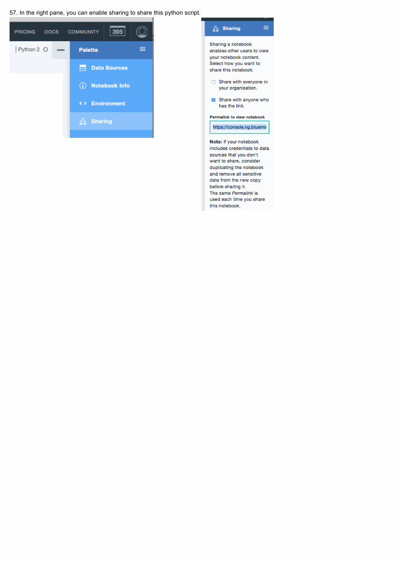
57. In the right pane, you can enable sharing to share this python script.

Part 6: Analyze data graphically using R Scripts 58. In the dashDB tab, on the left pane click “Analysis -> R Scripts”

59. In the new editor that opens click “+” sign to add a new table. Choose “<TABLE_NAME>”, check both columns, TIME and TEMP and click on Ok. Note that as the schema name is auto generated it will be different.

60. There is a new script that automatically gets loaded in the editor on the right pane. Delete it completely and type the following instead. Click “Submit” to run the script.

61. You can also save this script by clicking “Save” and naming it. It will show up in the pane on the left under “My Projects” tab.

62. If the “Submit” was successful, a PDF icon will appear instead of the script. Click to open Line Graph. The temperature can be matched with data in the table.

Part 7: Analyze data using Excel 63. Import CSV data into Excel

64. This data will now open into excel. Perform any statistical function on it, eg: Average of temperature

Congratulations! You’ve successfully analyzed temperature