Linear Algebra Review

Contents

1 Basic Concepts and Notations 2

2 Matrix Operations and Properties 32.1 Matrix Multiplication . . . . . . . . . . . . . . . . . . . . . . . . . . . . . . . . . . . . . . 3

2.1.1 Vector-Vector Products . . . . . . . . . . . . . . . . . . . . . . . . . . . . . . . . . 32.1.2 Matrix-Vector Products . . . . . . . . . . . . . . . . . . . . . . . . . . . . . . . . . 42.1.3 Matrix-Matrix Products . . . . . . . . . . . . . . . . . . . . . . . . . . . . . . . . . 52.1.4 Kronecker Products . . . . . . . . . . . . . . . . . . . . . . . . . . . . . . . . . . . 52.1.5 Block Matrix Products . . . . . . . . . . . . . . . . . . . . . . . . . . . . . . . . . . 6

2.2 The Transpose . . . . . . . . . . . . . . . . . . . . . . . . . . . . . . . . . . . . . . . . . . 62.3 Symmetric Matrices . . . . . . . . . . . . . . . . . . . . . . . . . . . . . . . . . . . . . . . 72.4 The Trace . . . . . . . . . . . . . . . . . . . . . . . . . . . . . . . . . . . . . . . . . . . . . 72.5 Vector Norms . . . . . . . . . . . . . . . . . . . . . . . . . . . . . . . . . . . . . . . . . . . 72.6 Vector Spaces . . . . . . . . . . . . . . . . . . . . . . . . . . . . . . . . . . . . . . . . . . . 82.7 Orthogonality . . . . . . . . . . . . . . . . . . . . . . . . . . . . . . . . . . . . . . . . . . . 82.8 The Rank . . . . . . . . . . . . . . . . . . . . . . . . . . . . . . . . . . . . . . . . . . . . . 92.9 Range and Nullspace . . . . . . . . . . . . . . . . . . . . . . . . . . . . . . . . . . . . . . . 102.10 QR Factorization . . . . . . . . . . . . . . . . . . . . . . . . . . . . . . . . . . . . . . . . . 102.11 Matrix Norms . . . . . . . . . . . . . . . . . . . . . . . . . . . . . . . . . . . . . . . . . . . 11

2.11.1 Induced Matrix Norms . . . . . . . . . . . . . . . . . . . . . . . . . . . . . . . . . . 112.11.2 General Matrix Norms . . . . . . . . . . . . . . . . . . . . . . . . . . . . . . . . . . 12

2.12 The Inverse . . . . . . . . . . . . . . . . . . . . . . . . . . . . . . . . . . . . . . . . . . . . 132.13 The Determinant . . . . . . . . . . . . . . . . . . . . . . . . . . . . . . . . . . . . . . . . . 142.14 Schur Complement . . . . . . . . . . . . . . . . . . . . . . . . . . . . . . . . . . . . . . . . 16

3 Eigenvalues and Eigenvectors 163.1 Definitions . . . . . . . . . . . . . . . . . . . . . . . . . . . . . . . . . . . . . . . . . . . . . 163.2 General Results . . . . . . . . . . . . . . . . . . . . . . . . . . . . . . . . . . . . . . . . . . 173.3 Spectral Decomposition . . . . . . . . . . . . . . . . . . . . . . . . . . . . . . . . . . . . . 18

3.3.1 Spectral Decomposition Theorem . . . . . . . . . . . . . . . . . . . . . . . . . . . . 183.3.2 Applications . . . . . . . . . . . . . . . . . . . . . . . . . . . . . . . . . . . . . . . 19

4 Singular Value Decomposition 194.1 Definitions and Basic Properties . . . . . . . . . . . . . . . . . . . . . . . . . . . . . . . . 194.2 Low-Rank Approximations . . . . . . . . . . . . . . . . . . . . . . . . . . . . . . . . . . . 204.3 SVD vs. Spectral Decomposition . . . . . . . . . . . . . . . . . . . . . . . . . . . . . . . . 22

225 Quadratic Forms and Definiteness

6 Matrix Calculus 246.1 Notations . . . . . . . . . . . . . . . . . . . . . . . . . . . . . . . . . . . . . . . . . . . . . 246.2 The Gradient . . . . . . . . . . . . . . . . . . . . . . . . . . . . . . . . . . . . . . . . . . . 246.3 The Hessian . . . . . . . . . . . . . . . . . . . . . . . . . . . . . . . . . . . . . . . . . . . . 256.4 Least Squares . . . . . . . . . . . . . . . . . . . . . . . . . . . . . . . . . . . . . . . . . . . 256.5 Digression: Generalized Inverse . . . . . . . . . . . . . . . . . . . . . . . . . . . . . . . . . 276.6 Gradients of the Determinant . . . . . . . . . . . . . . . . . . . . . . . . . . . . . . . . . . 276.7 Eigenvalues as Optimization . . . . . . . . . . . . . . . . . . . . . . . . . . . . . . . . . . . 286.8 General Derivatives of Matrix Functions . . . . . . . . . . . . . . . . . . . . . . . . . . . . 28

7 Bibliographic Remarks 29

1

1 Basic Concepts and Notations

We use the following notation:

• By A ∈ Rm×n we denote a matrix with m rows and n columns, where the entries of A are realnumbers.

• By x ∈ Rn, we denote a vector with n entries.

• An n-dimensional vector is often thought of as a matrix with n rows and 1 column, known ascolumn vector . A row vector is a matrix with 1 row and n columns, which we typically writexT (xT denote the transpose of x, which we will define shortly).

• The ith element of a vector x is denoted xi:

x =

x1x2...xn

.

• We use notation aij to denote the entry of A in the ith row and jth column:

A =

a11 a12 . . . a1na21 a22 . . . a2n...

.... . .

...am1 am2 . . . amn

= (aij).

• We denote the jth columns of A by aj :

A =

. . .a1 a2 . . . an

. . .

.• We denote the ith row of A by ai:

A =

aT(1)aT(2)

...aT(m)

or A =

aT1aT2...

aTm

.

• The meanings of the notations usually should be obvious from its use when they are ambiguous.

• A matrix written in terms of its sub-matrices is called a partitioned matrix :

A =

A11 A12 . . . A1q

A21 A12 . . . A2q

......

. . ....

Ap1 Ap2 . . . Apq

,where Aij ∈ Rr×s , m = pr, and n = qs. Based on the Matlab colon notation, we have Aij =A((i− 1)r + 1 : ir, (j − 1)s+ 1 : s

).

2

Table 1: Particular matrices and types of matrix

Name Definition Notation

Scalar m = n = 1 a, b . . .

Column vector n = 1 x,y . . .

All-ones vector [1, . . . , 1]T 1 or 1n

Null aij = 0 0

Square m = n A ∈ Rn×n

Diagonal m = n, aij = 0 if i 6= j diag(a11, . . . , ann) or diag([a11, . . . , ann]T )

Identity diag(1) I or In

Symmetric aij = aji A ∈ Sn

Table 2: Basic matrix operations

Operation Restrictions Notations and Definitions

Addition / Subtraction A,B of the same order A±B = (aij ± bij)Scalar multiplication cA = c(aij)

Inner product x,y of the same order xTy =∑xiyi

Multiplication #columns of A equals #rows of B AB = (aT(i)bj)

Kronecker Product A⊗B = (aijB)

Transpose AT = [a(1), . . . ,a(m)]

Trace A is square tr(A) =∑aii

Determinant A is square |A| or det(A)

Inverse A is sqaure and det(A) 6= 0 AA−1 = A−1A = I

Pseudo-inverse A†

2 Matrix Operations and Properties

2.1 Matrix Multiplication

The product of two matrices A ∈ Rm×n and B ∈ Rn×p is the matrix

C = AB ∈ Rm×p,

where

cij =

n∑k=1

aikbkj .

Note that in order for the matrix product to exist, the number of columns in A must equal the numberof rows in B. There are many ways of looking at matrix multiplication. We’ll start by examining a fewspecial cases.

2.1.1 Vector-Vector Products

Given two vectors x,y ∈ Rn, the quantity xTy, sometimes called the inner product or dot product ofthe vectors, is a real number given by

xTy ∈ R =[x1 x2 . . . xn

]y1y2...yn

=

n∑i=1

xiyi.

3

Note that it is always the case that xTy = yTx.Given x ∈ Rm,y ∈ Rn (not for the same size), xyT is called the outer product of the vectors. It is

a matrix whose entries are given by (xyT )ij = xiyj ,

xyT ∈ Rm×n =

x1x2...xn

[y1 y2 . . . yn]

=

x1y1 x1y2 . . . x1ynx2y1 x2y2 . . . x2yn

......

. . ....

xmy1 xmy2 . . . xmyn

.Consider the matrix A ∈ Rm×n whose columns are equal to some vector x ∈ Rm. Using outer products,we can represent A compactly as,

A =

x x . . . x

=

x1 x1 . . . x1x2 x2 . . . x2...

.... . .

...xm xm . . . xm

=

x1x2...xm

[1 1 . . . 1]

= x1T .

2.1.2 Matrix-Vector Products

Given a matrix A ∈ Rm×n and a vector x ∈ Rn, their product is a vector y = Ax ∈ Rm. There are acouple ways of looking at matrix-vector multiplication, and we will look at each of them in turn.

If we write A by rows, then we can express Ax as,

y = Ax =

aT(1)aT(2)

...aT(m)

x =

aT(1)x

aT(2)x...

aT(m)x

.In other words, the ith entry of y is equal to the inner product of the ith row of A and x, yi = aT(i)x.

Alternatively, lets write A in column form. In this case we see that,

y = Ax =

. . .a1 a2 . . . an

. . .

x1x2...xn

=

a1

x1 +

a2

x2 + · · ·+

an

xn.In other words, y is a linear combination of the columns of A, where the coefficients of the linearcombination are given by the entries of x.

So far we have been multiplying on the right by a column vector. We also have similar interpretationof multiplying on the left by a row vector. For A ∈ Rm×n and a vector x ∈ Rm, which gives

yT = xTA = xT

. . .a1 a2 . . . an

. . .

=

xTa1

xTa2

...xTan

,

yT = xTA

=[x1 x2 . . . xn

]

aT(1)aT(2)

...aT(m)

= x1

[aT(1)

]+ x2

[aT(2)

]+ · · ·+ xn

[aT(n)

].

4

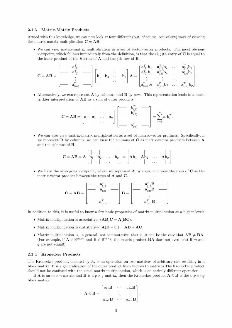
2.1.3 Matrix-Matrix Products

Armed with this knowledge, we can now look at four different (but, of course, equivalent) ways of viewingthe matrix-matrix multiplication C = AB.

• We can view matrix-matrix multiplication as a set of vector-vector products. The most obviousviewpoint, which follows immediately from the definition, is that the (i, j)th entry of C is equal tothe inner product of the ith row of A and the jth row of B.

C = AB =

aT(1)aT(2)

...aT(m)

. . .

b1 b2 . . . bp. . .

A =

aT(1)b1 aT(1)b2 . . . aT(1)bpaT(2)b1 aT(2)b2 . . . aT(2)bp

......

. . ....

aT(m)b1 aT(m)b2 . . . aT(m)bp

.

• Alternatively, we can represent A by columns, and B by rows. This representation leads to a muchtrickier interpretation of AB as a sum of outer products.

C = AB =

. . .a1 a2 . . . an

. . .

bT(1)bT(2)

...bT(n)

=

n∑i=1

aibTi .

• We can also view matrix-matrix multiplication as a set of matrix-vector products. Specifically, ifwe represent B by columns, we can view the columns of C as matrix-vector products between Aand the columns of B.

C = AB = A

. . .b1 b2 . . . bp

. . .

=

. . .Ab1 Ab2 . . . Abp

. . .

• We have the analogous viewpoint, where we represent A by rows, and view the rows of C as the

matrix-vector product between the rows of A and C.

C = AB =

aT(1)aT(2)

...aT(m)

B =

aT(1)B

aT(2)B...

aT(m)B

In addition to this, it is useful to know a few basic properties of matrix multiplication at a higher level:

• Matrix multiplication is associative: (AB)C = A(BC).

• Matrix multiplication is distributive: A(B + C) = AB + AC.

• Matrix multiplication is, in general, not commutative; that is, it can be the case that AB 6= BA.(For example, if A ∈ Rm×n and B ∈ Rm×q, the matrix product BA does not even exist if m andq are not equal!)

2.1.4 Kronecker Products

The Kronecker product, denoted by ⊗, is an operation on two matrices of arbitrary size resulting in ablock matrix. It is a generalization of the outer product from vectors to matrices The Kronecker productshould not be confused with the usual matrix multiplication, which is an entirely different operation.

If A is an m× n matrix and B is a p× q matrix, then the Kronecker product A⊗B is the mp× nqblock matrix:

A⊗B =

a11B · · · a1nB...

. . ....

am1B · · · amnB

,5

more explicitly:

A⊗B =

a11b11 a11b12 · · · a11b1q · · · · · · a1nb11 a1nb12 · · · a1nb1qa11b21 a11b22 · · · a11b2q · · · · · · a1nb21 a1nb22 · · · a1nb2q

......

. . ....

......

. . ....

a11bp1 a11bp2 · · · a11bpq · · · · · · a1nbp1 a1nbp2 · · · a1nbpq...

......

. . ....

......

......

.... . .

......

...am1b11 am1b12 · · · am1b1q · · · · · · amnb11 amnb12 · · · amnb1qam1b21 am1b22 · · · am1b2q · · · · · · amnb21 amnb22 · · · amnb2q

......

. . ....

......

. . ....

am1bp1 am1bp2 · · · am1bpq · · · · · · amnbp1 amnbp2 · · · amnbpq

.

The following properties of transposes are easily verified:

• A⊗ (B + C) = A⊗B + A⊗C.

• (A⊗B)⊗C = A⊗ (B⊗C).

• (A⊗B)(C⊗D) = AC⊗BD.

• tr(A⊗B) = tr(A)tr(B).

2.1.5 Block Matrix Products

A block partitioned matrix product can sometimes be used on submatrices forms. The partitioning ofthe factors is not arbitrary, however, and requires conformable partitions between two matrices such thatall submatrix products that will be used are defined. Given a matrix A ∈ Rm×p with q row partitionsand s column partitions

A =

A11 A12 · · · A1s

A21 A22 · · · A2s

......

. . ....

Aq1 Aq2 · · · Aqs

and B ∈ Rp×n with s row partitions and r column partitions

B =

B11 B12 · · · B1r

B21 B22 · · · B2r

......

. . ....

Bs1 Bs2 · · · Bsr

,that are compatible with the partitions of A, the matrix product C = AB can be formed blockwise,yielding as an matrix with q row partitions and r column partitions. The matrices in your matrix C arecalculated by multiplying

Cij =

s∑k=1

AikBkj .

2.2 The Transpose

The transpose of a matrix results from flipping the rows and columns. Given a matrix A ∈ Rm×n, itstranspose, written AT ∈ Rn×m, is the n×m matrix whose entries are given by (AT )ij = Aji. We havein fact already been using the transpose when describing row vectors, since the transpose of a columnvector is naturally a row vector. The following properties of transposes are easily verified:

• (AT )T = A

• (AB)T = BTAT

6

• (A + B)T = AT + BT

Sometimes, we also use quotation marks A′ to express the transpose of A. But note that the quotation inMatlab is to express the hermitian conjugate (notated as A∗), not transpose. The transpose operationin Matlab should be written as dot quotation.

2.3 Symmetric Matrices

A square matrix A ∈ Rn×n is symmetric if A = AT . It is anti-symmetric if A = −AT . It is easyto show that for any matrix A ∈ Rn×n, the matrix A−AT is anti-symmetric. From this it follows thatany square matrix A ∈ Rn×n can be represented as a sum of a symmetric matrix and an anti-symmetricmatrix, since

A =1

2(A + AT ) +

1

2(A−AT )

and the first matrix on the right is symmetric, while the second is anti-symmetric. It turns out thatsymmetric matrices occur a great deal in practice, and they have many nice properties which we willlook at shortly. It is common to denote the set of all symmetric matrices of size n as Sn, so that A ∈ Snmeans that A is a symmetric n × n matrix. Another property is that for A ∈ Sn,x ∈ Rn, y ∈ Rn, wehave xTAy = yTAx, which can be verified easily.

2.4 The Trace

The trace of a square matrix A ∈ Rn×n, denoted tr(A) (or just trA if the parentheses are obviouslyimplied), is the sum of diagonal elements in the matrix:

trA =

n∑i=1

aii.

The trace has the following properties:

• For A ∈ Rn×n, trA = trAT .

• For A,B ∈ Rn×n, tr(A±B) = trA± trB.

• For A ∈ Rn×n, c ∈ R, tr(cA) = ctrA.

• For A,B such that AB is square, trAB = trBA.

• For A,B,C such that ABC is square, trABC = trBCA = trCAB, and so on for the product ofmore matrices.

• For A ∈ Rn×n, tr(ATA) =

n∑i=1

n∑j=1

a2ij .

The fourth equality, where the main work occurs, uses the commutativity of scalar multiplication inorder to reverse the order of the terms in each product, and the commutativity and associativity of scalaraddition in order to rearrange the order of the summation.

2.5 Vector Norms

A norm of a vector x ∈ Rn written by ||x||, is informally a measure of the length of the vector. Forexample, we have the commonly-used Euclidean norm (or `2 norm),

||x||2 =√

xTx =

√√√√ n∑i=1

x2i .

More formally, a norm is any function Rn → R that satisfies 4 properties:

1. For all x ∈ Rn, ||x|| ≥ 0 (non-negativity).

2. ||x|| = 0 if and only if x = 0 (definiteness).

7

3. For all x ∈ Rn, t ∈ R, ||tx|| = |t|||x|| (homogeneity).

4. For all x,y ∈ Rn, ||x + y|| ≤ ||x||+ ||y|| (triangle inequality).

Other examples of norms are the `1 norm,

||x||1 =

n∑i=1

|xi|,

and the `∞ norm,

||x||∞ = maxi|xi|.

In fact, all three norms presented so far are examples of the family of `p norms, which are parameterizedby a real number p ≥ 1, and defined as

||x||p =( n∑i=1

|xi|p)1/p

.

2.6 Vector Spaces

The set of vectors in Rm satisfies the following properties for all x,y ∈ Rm and all a, b ∈ R.

• a(x + y) = ax + ay

• (a+ b)x = ax + bx

• (ab)x = a(by)

• 1x = x

If W is a subset of Rm such that for all x,y ∈ W and a ∈ R have a(x + y) ∈ W, then W is called avector subspace of Rm. Two simple examples of subspace of Rm are {0} and Rm itself.

A set of vectors {x1,x2, . . . ,xn} ⊂ Rm is said to be linearly independent if no vector can berepresented as a linear combination of the remaining vectors. Conversely, if one vector belonging to theset can be represented as a linear combination of the remaining vectors, then the vectors are said to belinear dependent . That is, if

xn =

n−1∑i=1

αixi

for some scalar values α1, . . . , αn−1, then we say that the vectors x1,. . . ,xn are linearly dependent;otherwise the vectors are linearly independent.

Let W be a subspace of Rn. Then a basis of W is a maximal linear independent set of vectors. Thefollowing properties hold for a basis of W:

• Every basis of W contains the same number of elements. This number is called the dimension ofW and denoted dim(W). In particular dim(Rn) = n.

• If x1, . . . ,xk is a basis for W then every element x ∈ W can be express as a linear combination ofx1, . . . ,xk.

2.7 Orthogonality

Two vectors x,y ∈ Rn are orthogonal if xTy = 0. A vector x ∈ Rn is normalized if ||x||2 = 1. Asquare matrix U ∈ Rn×n is orthogonal (note the different meanings when talking about vectors versusmatrices) if all its columns are orthogonal to each other and are normalized (the columns are then referredto as being orthonormal). It follows immediately from the definition of orthogonality and normality that

UTU = I = UUT .

Note that if U is not square, i.e., U ∈ Rm×n, n < m, but its columns are still orthonormal, then UTU = I,but UUT 6= I, we call that U is column orthonormal .

8

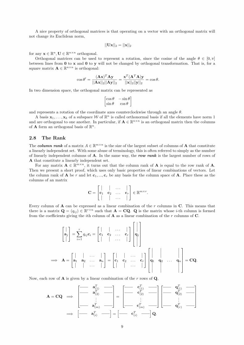
A nice property of orthogonal matrices is that operating on a vector with an orthogonal matrix willnot change its Euclidean norm,

||Ux||2 = ||x||2

for any x ∈ Rn,U ∈ Rn×n orthogonal.Orthogonal matrices can be used to represent a rotation, since the cosine of the angle θ ∈ [0, π]

between lines from 0 to x and 0 to y will not be changed by orthogonal transformation. That is, for asquare matrix A ∈ Rn×n is orthogonal:

cos θ′ =(Ax)TAy

||Ax||2||Ay||2=

xT (ATA)y

||x||2||y||2= cos θ.

In two dimension space, the orthogonal matrix can be represented as[cos θ − sin θsin θ cos θ

]and represents a rotation of the coordinate axes counterclockwise through an angle θ.

A basis x1, . . . ,xk of a subspace W of Rn is called orthonormal basis if all the elements have norm 1and are orthogonal to one another. In particular, if A ∈ Rn×n is an orthogonal matrix then the columnsof A form an orthogonal basis of Rn.

2.8 The Rank

The column rank of a matrix A ∈ Rm×n is the size of the largest subset of columns of A that constitutea linearly independent set. With some abuse of terminology, this is often referred to simply as the numberof linearly independent columns of A. In the same way, the row rank is the largest number of rows ofA that constitute a linearly independent set.

For any matrix A ∈ Rm×n, it turns out that the column rank of A is equal to the row rank of A.Then we present a short proof, which uses only basic properties of linear combinations of vectors. Letthe column rank of A be r and let c1, ..., cr be any basis for the column space of A. Place these as thecolumns of an matrix

C =

. . .c1 c2 . . . cr

. . .

∈ Rm×r.

Every column of A can be expressed as a linear combination of the r columns in C. This means thatthere is a matrix Q = (qij) ∈ Rr×n such that A = CQ. Q is the matrix whose i-th column is formedfrom the coefficients giving the ith column of A as a linear combination of the r columns of C.

aj

=

r∑i=1

qijci =

. . .c1 c2 . . . cr

. . .

qj

=⇒ A =

. . .a1 a2 . . . an

. . .

=

. . .c1 c2 . . . cr

. . .

q1 q2 . . . qn

= CQ.

Now, each row of A is given by a linear combination of the r rows of Q,

A = CQ =⇒

aT(1)aT(2)

...aT(m)

=

cT(1)cT(2)

...cT(m)

qT(1)qT(2)

...qT(r)

=⇒

[aT(i)

]=[

cT(i)

]Q.

9

Therefore, the row rank of A cannot exceed r. This proves that the row rank of A is less than or equalto the column rank of A. This result can be applied to any matrix, so apply the result to the transposeof A. Since the row rank of the transpose of A is the column rank of A and the column rank of thetranspose of A is the row rank of A, this establishes the reverse inequality and we obtain the equality ofthe row rank and the column rank of A, so both quantities are referred to collectively as the rank of A,denoted as rank(A).

The following are some basic properties of the rank:

• For A ∈ Rm×n, rank(A) ≤ min(m,n). If rank(A) = min(m,n), then A is said to be full rank.

• For A ∈ Rm×n, rank(A) = rank(AT ).

• For A ∈ Rm×n,B ∈ Rn×p, rank(AB) ≤ min(rank(A), rank(B)).

• For A,B ∈ Rm×n, rank(A + B) ≤ rank(A) + rank(B).

2.9 Range and Nullspace

The span of a set of vectors {x1, . . . ,xn} is the set of all vectors that can be expressed as a linearcombination of {x1, . . . ,xn}. That is,

span({x1, . . . ,xn}) =

{v : v =

n∑i=1

αixi, αi ∈ R

}.

The range (also called the column space) of matrix A ∈ Rm×n denote R(A). In other words,

R(A) = {v ∈ Rm : v = Ax,x ∈ Rn}.

The nullspace of a matrix A ∈ Rm×n, denoted N (A) is the set of all vectors that equal 0 whenmultiplied by A,

N (A) = {x ∈ Rn : Ax = 0}.

Note that vectors in R(A) are of size m, while vectors in the N (A) are of size n, so vectors in R(AT )and N (A) are both in Rn. In fact, we can say much more that

{w : w = u+ v, u ∈ R(AT ), v ∈ N (A)} = Rn and R(AT ) ∩N (A) = {0}.

In other words, R(AT ) and N (A) together span the entire space of Rn. Furthermore, the Table 3summarizes some properties of four fundamental subspace of A including the range and the nullspace,where A has singular value decomposition1:

A = UΣVT .

Table 3: Properties of four fundamental subspaces of rank r matrix A ∈ Rm×n

Name of Subspace Notation Containing Space Dimension Basis

range, column space or image R(A) Rm r (rank) The first r columns of U

nullspace or kernel N (A) Rn n− r (nullity) The last (n− r) columns of V

row space or coimage R(AT ) Rn r (rank) The first r columns of V

left nullspace or cokernel N (AT ) Rm m− r (corank) The last (m− r) columns of U

2.10 QR Factorization

Given a full rank matrix A ∈ Rm×n (m ≥ n), we can construct the vectors q1, . . . ,qn and entries rijsuch that

A =

. . .a1 a2 . . . an

. . .

=

. . .q1 q2 . . . qn

. . .

r11 r12 . . . r1n

r22 . . . r2n. . .

...rnn

,1Singular value decomposition will be introduced in section 4.

10

where the diagonal entries rkk are nonzero, then a1, . . . ,ak can be expressed as linear combinationof q1, . . . ,qk and the invertibility of the upper-left k × k block of the triangular matrix implies that,conversely, q1, . . . ,qk can be expressed as linear combination of a1, . . . ,ak. Written out, these equationstake the form

a1 = r11q1

a2 = r12q1 + r22q2

a3 = r13q1 + r23q2 + r33q3

...

an = r1nq1 + r2nq2 + · · ·+ rnnqn

As matrix formula, we have

A = QR,

where Q is m× n with orthonormal columns and R is n× n and upper-triangular. Such a factorizationis called a reduced QR factorization of A.

A full QR factorization of A ∈ Rm×n (m ≥ n) goes futher, appending an additional m − n

orthogonal columns to Q so that it becomes an m × m orthogonal matrix Q. In the process, rows ofzeros are appended to R so that it becomes an m× n matrix R. Then we have

A = QR.

There is an old idea, known as Gram-Schmidt orthogonalization to construct the vectors q1 . . . ,qnand entires rij for reduced QR factorization. Let’s rewrite the relationship between q1 . . . ,qn anda1 . . . ,an, in the form

q1 =a1

r11

q2 =a2 − r12q1

r22

q3 =a3 − r13q1 − r23q2

r33...

qn =an −

∑n−1i=1 rinqirnn

.

Let rij = qTi aj for i 6= j, and |rjj | = ||aj −∑j−1i=1 rijqi||2, then we have qTi qj = 0 (can be proved by

induction). But how to obtain full QR factorization?

2.11 Matrix Norms

2.11.1 Induced Matrix Norms

An m × n matrix can be viewed as a vector in an mn-dimensional space: each of the mn entries of thematrix is an independent coordinate. Any mn-dimensional norm can therefore be used for measuringthe ‘size’ of such a matrix. In dealing with a space of matrices, these are the induced matrix norms,defined in terms of the behavior of a matrix as an operator between its normed domain and range space.

Given vector norms || · ||(m), || · ||(n) and on the domain and the range of A ∈ Rm×n, respectively, theinduced matrix norm ||A||(m,n) is the smallest number C for which the following inequality holds for allx ∈ Rn:

||Ax||(m) ≤ C||x||(n).

The induced matrix norm can be defined equivalently as following:

||A||(m,n) = supx∈Rn,x 6=0

||Ax||(m)

||x||(n)= sup

x∈Rn,||x||=1

||Ax||(m).

11

Note that the (m) and (n) in subscript are only represented the dimensionality of vectors, rather than`m or `n norm. The notations || · ||(m) and || · ||(n) can be any the same type of vector norm.

For example, if A ∈ Rm×n, then its 1-norm ||A||1 is equal to the ‘maximum column sum’ of A. Weexplain and derive this result as follows. Let’s write A in terms of its columns

A =

. . .a1 a2 . . . an

. . .

.Any vector x in the set {x ∈ Rn :

∑ni=1 |xi| = 1} satisfies

||Ax||1 =∥∥∥ n∑i=1

xiai

∥∥∥1≤

n∑i=1

|xi|||ai|| ≤n∑i=1

|xi|(

max1≤j≤n

||aj ||1)

= max1≤j≤n

||aj ||1.

By choosing x be the vector whose jth entry is 1 and others are zero, where j maximizes ||aj ||1, we attainthis bound, and thus the matrix norm is

||A||1 = max1≤j≤n

||aj ||1.

By much the same argument, it can be shown that the ∞-norm of an m × n matrix is equal to the‘maximum row sum’

||A||∞ = max1≤i≤m

||a(i)||1.

Computing matrix p-norms with p 6= 1,∞ is more difficult.Then we provide a geometric example of some induced matrix norms. Let’s consider the matrix

A =

[1 20 2

],

which maps R2 to R2 by multiplication.Figure 1 depicts the action of A on the unit balls of R2 defined by the 1-, 2- and∞-norms. Regardless

of the norm, A maps e1 = [1, 0]T to the first column of A itself, and e2 = [0, 1]T to the second columnof A.

In the 1-norm, the vector whose norm is 1 that is amplified most by A is [0, 1]T (or its negative), andthe amplification factor is 4. In the ∞-norm, the vector whose norm is 1 that is amplified most by A is[1, 1]T (or its negative), and the amplification factor is 3. In the 2-norm, the vector whose norm is 1 thatis amplified most by A is [0, 1]T is the vector indicated by the dash line in the figure (or its negative),

and the amplification factor is approximately 2.9208 (the exact value is√

(9 +√

65)/2). We will consider

how to get 2-norm again in section 3.3.2.

2.11.2 General Matrix Norms

Matrix norms do not have to be induced by vector norms. In general a matrix norm must merely satisfythe vector norm conditions applied in the mn-dimensional vector space of matrices:

1. For all A ∈ Rm×n, ||A|| ≥ 0 (non-negativity).

2. ||A|| = 0 if and only if aij = 0. (definiteness).

3. For all A ∈ Rm×n, t ∈ R, ||tA|| = |t|||A|| (homogeneity).

4. For all A,B ∈ Rm×n, ||A + B|| ≤ ||A||+ ||B|| (triangle inequality).

The most important matrix norm which is not induced by a vector norm is Frobenius norm (or F-norm),for A ∈ Rm×n, defined by

||A||F =√

tr(ATA) =

√√√√ m∑i=1

n∑j=1

a2ij .

12

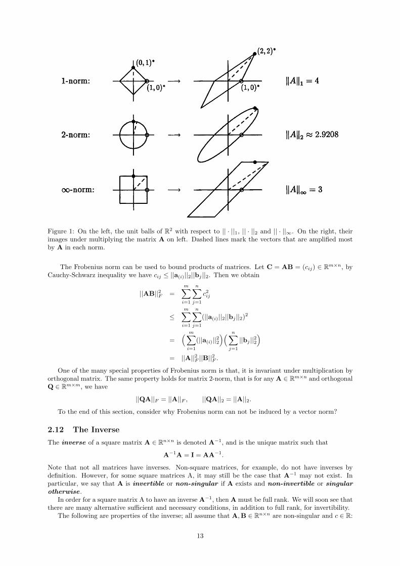
Figure 1: On the left, the unit balls of R2 with respect to || · ||1, || · ||2 and || · ||∞. On the right, theirimages under multiplying the matrix A on left. Dashed lines mark the vectors that are amplified mostby A in each norm.

The Frobenius norm can be used to bound products of matrices. Let C = AB = (cij) ∈ Rm×n, byCauchy-Schwarz inequality we have cij ≤ ||a(i)||2||bj ||2. Then we obtain

||AB||2F =

m∑i=1

n∑j=1

c2ij

≤m∑i=1

n∑j=1

(||a(i)||2||bj ||2)2

=( m∑i=1

(||a(i)||22)( n∑

j=1

||bj ||22)

= ||A||2F ||B||2F .

One of the many special properties of Frobenius norm is that, it is invariant under multiplication byorthogonal matrix. The same property holds for matrix 2-norm, that is for any A ∈ Rm×n and orthogonalQ ∈ Rm×m, we have

||QA||F = ||A||F , ||QA||2 = ||A||2.

To the end of this section, consider why Frobenius norm can not be induced by a vector norm?

2.12 The Inverse

The inverse of a square matrix A ∈ Rn×n is denoted A−1, and is the unique matrix such that

A−1A = I = AA−1.

Note that not all matrices have inverses. Non-square matrices, for example, do not have inverses bydefinition. However, for some square matrices A, it may still be the case that A−1 may not exist. Inparticular, we say that A is invertible or non-singular if A exists and non-invertible or singularotherwise .

In order for a square matrix A to have an inverse A−1, then A must be full rank. We will soon see thatthere are many alternative sufficient and necessary conditions, in addition to full rank, for invertibility.

The following are properties of the inverse; all assume that A,B ∈ Rn×n are non-singular and c ∈ R:

13

• (A−1)−1 = A

• (cA)−1 = c−1A−1

• (A−1)T = (AT )−1

• (AB)−1 = B−1A−1

• A−1 = AT if A ∈ Rn×n is orthogonal matrix.

Additionally, if all the necessary inverse exist, then for A ∈ Rn×n, B ∈ Rn×p, C ∈ Rp×p and D ∈ Rp×n,the Woodbury matrix identity says that

(A + BCD)−1 = A−1 −A−1B(C−1 + DA−1B)−1DA−1.

This conclusion is very useful to compute inverse of matrix more efficiently when A = I and n� p.For non-singular matrix A ∈ Rn×n and vectors x,b,∈ Rn, when writing the product x = A−1b it is

important not to let the inverse matrix notation obscure what is really going on! Rather than thinkingof x as the result of applying A−1 to b, we should understand it as the unique vector that satisfies theequation Ax = b. This means that x is the vector of coefficients of the unique linear expansion of b inthe basis of columns of A. Multiplication by A−1 is a change of basis operation as Figure 2 displayed.

Figure 2: The vector ei represent the vector in Rn whose ith entry is 1 and the others are 0.

2.13 The Determinant

The determinant of a square matrix A ∈ Rn×n, is a function det : Rn×n → R and is denoted det(A)or |A|. (like the trace operator, we usually omit parentheses). Algebraically, one could write down anexplicit formula for the determinant of A, but this unfortunately gives little intuition about its meaning.Instead, well start out by providing a geometric interpretation of the determinant and then visit some ofits specific algebraic properties afterwards. Given a square matrix

A =

aT(1)aT(2)

...aT(m)

,consider the set of points S ⊂ Rn formed by taking all possible linear combinations of the row vectors,where the coefficients of the linear combination are all between 0 and 1; that is, the set S is the restrictionof span({a1, ...,an}) to only those linear combinations whose coefficients satisfy 0 ≤ αi ≤ 1, i = 1, . . . , n.Formally, we have

S = {v ∈ Rn : v =

n∑i=1

αiai, where 0 ≤ αi ≤ 1, i = 1, . . . , n}.

The absolute value of the determinant of A, it turns out, is a measure of the ‘volume’ 2 of the set S.For example, consider the 2× 2 matrix,

A =

[1 33 2

].

2Admittedly, we have not actually defined what we mean by ‘volume’ here, but hopefully the intuition should be clearenough. When n = 2, our notion of ‘volume’ corresponds to the area of S in the Cartesian plane. When n = 3, ‘volume’corresponds with our usual notion of volume for a three-dimensional object.

14

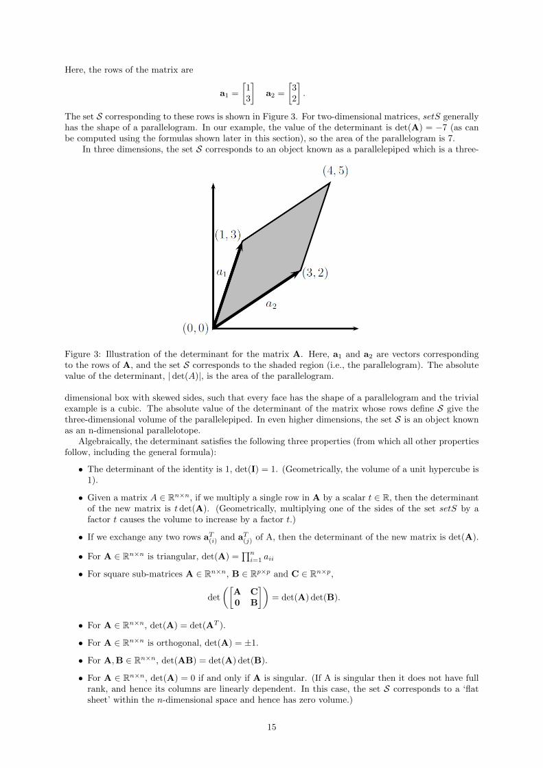
Here, the rows of the matrix are

a1 =

[13

]a2 =

[32

].

The set S corresponding to these rows is shown in Figure 3. For two-dimensional matrices, setS generallyhas the shape of a parallelogram. In our example, the value of the determinant is det(A) = −7 (as canbe computed using the formulas shown later in this section), so the area of the parallelogram is 7.

In three dimensions, the set S corresponds to an object known as a parallelepiped which is a three-

Figure 3: Illustration of the determinant for the matrix A. Here, a1 and a2 are vectors correspondingto the rows of A, and the set S corresponds to the shaded region (i.e., the parallelogram). The absolutevalue of the determinant, |det(A)|, is the area of the parallelogram.

dimensional box with skewed sides, such that every face has the shape of a parallelogram and the trivialexample is a cubic. The absolute value of the determinant of the matrix whose rows define S give thethree-dimensional volume of the parallelepiped. In even higher dimensions, the set S is an object knownas an n-dimensional parallelotope.

Algebraically, the determinant satisfies the following three properties (from which all other propertiesfollow, including the general formula):

• The determinant of the identity is 1, det(I) = 1. (Geometrically, the volume of a unit hypercube is1).

• Given a matrix A ∈ Rn×n, if we multiply a single row in A by a scalar t ∈ R, then the determinantof the new matrix is tdet(A). (Geometrically, multiplying one of the sides of the set setS by afactor t causes the volume to increase by a factor t.)

• If we exchange any two rows aT(i) and aT(j) of A, then the determinant of the new matrix is det(A).

• For A ∈ Rn×n is triangular, det(A) =∏ni=1 aii

• For square sub-matrices A ∈ Rn×n, B ∈ Rp×p and C ∈ Rn×p,

det

([A C0 B

])= det(A) det(B).

• For A ∈ Rn×n, det(A) = det(AT ).

• For A ∈ Rn×n is orthogonal, det(A) = ±1.

• For A,B ∈ Rn×n, det(AB) = det(A) det(B).

• For A ∈ Rn×n, det(A) = 0 if and only if A is singular. (If A is singular then it does not have fullrank, and hence its columns are linearly dependent. In this case, the set S corresponds to a ‘flatsheet’ within the n-dimensional space and hence has zero volume.)

15

Before giving the general definition for the determinant, we define, for A ∈ Rn×n,A\i,\j ∈ R(n−1)×(n−1)

to be the matrix that results from deleting the ith row and jth column from A. The general (recursive)formula for the determinant is

det(A) =

n∑i=1

(−1)i+jaij det(A\i,\j) (for any j ∈ {1, 2, . . . , n})

=

n∑j=1

(−1)i+jaij det(A\i,\j) (for any i ∈ {1, 2, . . . , n})

with the initial case that det(A) = a11 for A ∈ R1×1. If we were to expand this formula completelyfor A ∈ Rn×n, there would be a total of n (n factorial) different terms. For this reason, we hardly everexplicitly write the complete equation of the determinant for matrices bigger than 3 × 3. The classicaladjoint (often just called the adjoint) of a matrix A ∈ Rn×n is denoted adj(A), and defined as

adj(A) ∈ Rn×n,(adj(A)

)ij

= (−1)i+j det(A\j,\i)

(note the switch in the indices A\j,\i). It can be shown that for any nonsingular A ∈ Rn×n,

A−1 =1

det(A)adj(A).

2.14 Schur Complement

Suppose A ∈ Rp×p, B ∈ Rp×q, C ∈ Rq×p, D ∈ Rq×q, and D is invertible. Let

M ∈ R(p+q)×(p+q) =

[A BC D

].

Then the Schur complement of the block D of the matrix M is the matrix

A−BD−1C ∈ Rp×p.

This is analogous to an LDU decomposition . That is, we have shown that[A BC D

]=

[Ip BD−1

0 Iq

] [A−BD−1C 0

0 D

] [Ip 0

D−1C Iq

].

and the he inverse of M may be expressed involving D−1 and the inverse of Schur complement (if itexists) such as[

A BC D

]−1=

[Ip 0

−D−1C Iq

] [(A−BD−1C)−1 0

0 D−1

] [Ip −BD−1

0 Iq

]

=

[(A−BD−1C)−1 −(A−BD−1C)−1BD−1

−D−1C(A−BD−1C)−1 D−1 + D−1C(A−BD−1C)BD−1

].

Moreover, the determinant of M is also clearly seen to be given by

det(M) = det(D) det(A−BD−1C).

3 Eigenvalues and Eigenvectors

3.1 Definitions

Given a square matrix A ∈ Rn×n, we say that λ ∈ C is an eigenvalue of A and x ∈ Cn is thecorresponding eigenvector is the corresponding eigenvector if

Ax = λx, x 6= 0.

Intuitively, this definition means that multiplying A by the vector x results in a new vector that pointsin the same direction as x, but scaled by a factor λ. Also note that for any eigenvector x ∈ Cn, and

16

scalar t ∈ C,A(cx) = cAx = cλx = λ(cx), so cx is also an eigenvector. And if x and y are eigenvectorsfor λj and α ∈ R, then x + y and αx are also eigenvectors for λi. Thus, the set of all eigenvectors for λjforms a subspace which is called eigenspace of A for λi.

For this reason when we talk about ‘the’ eigenvector associated with λ, we define the standardizedeigenvector which are normalized to have length 1 (this still creates some ambiguity, since x and −x willboth be eigenvectors, but we will have to live with this). Sometimes we also use the term ‘eigenvector’to refer the standardized eigenvector .

We can rewrite the equation above to state that (λ,x) is an eigenvalue-eigenvector pair of A if,

(λI−A)x = 0, x 6= 0.

(λI −A)x = 0 has non-zero solution to x if and only if (λI −A)x has a non-zero dimension nullspace.

Considering that Table 3 implies rank(N (λI−A)

)= n− rank(λI−A), which means such x exists only

the case if (λI−A) is singular, that is

det(λI−A) = 0.

We can now use the previous definition of the determinant to expand this expression into a (verylarge) characteristic polynomial in λ, defined as

pA(λ) = det(A− λI) =

n∏i=1

(λi − λ),

where λ will have maximum degree n. We can find the n roots (possibly complex) of pA(λ) to find then eigenvalues λ1, . . . , λn. To find the eigenvector corresponding to the eigenvalue λi, we simply solve thelinear equation (λI−A)x = 0. It should be noted that this is not the method which is actually used inpractice to numerically compute the eigenvalues and eigenvectors (remember that the complete expansionof the determinant has n! terms), although it maybe works in the linear algebra exam you have taken.

3.2 General Results

The following are properties of eigenvalues and eigenvectors (in all cases assume A ∈ Rn×n has eigenvaluesλi, . . . , λn and associated eigenvectors x1, . . . ,xn):

• The trace of a A is equal to the sum of its eigenvalues,

tr(A) =

n∑i=1

λi.

• The determinant of A is equal to the product of its eigenvalues,

det(A) =

n∏i=1

λi.

• Let C ∈ Rn×n be a non-singular matrix, then

det(A− λI) = det(C) det(A− λIC−1C) det(C−1) = det(CAC−1 − λI).

Thus A and CAC−1 have the same eigenvalues and we call they are similar. Further, if xi is aneigenvector of A for λi then Cxi is an eigenvector of CAC−1 for λi.

• Let λ1 denote any particular eigenvalue of A, with eigenspaceW of dimension r (called geometricmultiplicity). If k denotes the multiplicity of λ1 in as a root of pA(λ) (called algebra multiplic-ity), then 1 ≤ r ≤ k

To prove the last conclusion, let e1, . . . , er be an orthogonal basis ofW and extend it to an orthogonalbasis of Rn, e1, . . . , er, f1, . . . , fn−r. Write E = [e1, . . . , er] and F = [f1, . . . , fn−r]. Then [E,F] is anorthogonal matrix so that

In = [E,F][E,F]T = EET + FFT ,

det([E,F][E,F]T ) = det([E,F]) det([E,F]T ) = 1,

ETAE = λ1ETE = λ1Ir,

FTF = In−r,

FTAE = λ1FTE = 0.

17

Thus

pA(λ) = det(A− λIn) = det([E,F]T ) det(A− λIn) det([E,F])

= det([E,F]T (AEET + AFFT − λEET − λFFT )[E,F])

= det

([(λ1 − λ)Ir ETAF

0 FTAF− λIn−r

])= (λ1 − λ)rpA1(λ),

then the multiplicity of λ1 as a root of pA(λ) is at least r. In section 3.3.1, we will show that if A issymmetric then r = k. However, if A is not symmetric, it is possible that r < k, For example,

A =

[0 10 0

]has eigenvalue 0 with multiplicity 2 but the corresponding eigenspace which is generated by [1, 0]T onlyhas dimension 1.

3.3 Spectral Decomposition

3.3.1 Spectral Decomposition Theorem

Two remarkable properties come about when we look at the eigenvalues and eigenvectors of symmetricmatrix A ∈ Sn. First, it can be shown that all the eigenvalues of A are real. Let an eigenvalue-eigenvectorpair (λ,x) of A, where x = y + iz and y, z ∈ Rn. Then we have

Ax = λx

=⇒ A(y + iz) = λ(y + iz)

=⇒ (y − iz)TA(y + iz) = λ(y − iz)T (y + iz)

=⇒ yTAy − izTAy + iyTAz + zTAz = λ(yTy + zT z)

=⇒ λ =yTAy + zTAz

yTy + zT z∈ R.

Secondly, two eigenvectors corresponding to distinct eigenvalues of A are orthogonal. In other words ifλi 6= λj are eigenvalues of A with eigenvector xi and xj respectively, then

λjxTi xj = xTi Axj = xTj Axi = λix

Tj xi,

so that xTi xj = 0, which means the eigenspaces of distinct eigenvalues are orthogonal.Furthermore, if λi is an eigenvector of A with m ≥ 2 algebra multiplicity, we can find m orthogonal

eigenvectors in its eigenspace. Then we prove this result. Let xi be one of eigenvector with λi and extendxi to an orthogonal bias xi,y2, . . . ,yn. and denote B = [xi,Y], where Y = [y2, . . . ,yn]. Then B isorthogonal and Y is column orthonormal, and we have

BTAB =

[λi 00 YTAY

]and

det(λIn −A) = det(BT ) det(λIn −A) det(B)

= det(λIn −BTAB)

= (λ− λi) det(λIn−1 −YTAY)

Since m ≥ 2, det(λiIn−1 −YTAY) must be zero, which means λi is an eigenvalue of YTAY. Supposexi2 is the eigenvector of YTAY with λi, then YTAYxi2 = λ2xi2. Hence, we have

BTAB

[0

xi2

]=

[λi 00 YTAY

] [0

xi2

]= λi

[0

xi2

]

=⇒ AB

[0

xi2

]= λiB

[0

xi2

]

18

which implies

xj = B

[0

xi2

]another eigenvectors of A and xTi xj = 0. Repeat this type of procedure by induction with B2 =[xi,xj ,y3, . . . ,yn], we can find m m orthogonal eigenvectors in this eigenspace.

Based on previous results, we can derive spectral decomposition theorem that any symmetricmatrix A ∈ Rn×n can be written as

A = XΛXT =

n∑i=1

λixixTi ,

where Λ = diag(λ1, . . . , λn) is a diagonal matrix of eigenvalues of A, and X is an orthogonal matrixwhose columns are corresponding standardized eigenvectors.

3.3.2 Applications

An application where eigenvalues and eigenvectors come up frequently is in maximizing some function ofa matrix. In particular, for a matrix A ∈ Sn, consider the following maximization problem,

maxx∈Rn

xTAx subject to ||x||22 = 1

i.e., we want to find the vector (of `2-norm 1) which maximizes the objective function (which is aquadratic form). Assuming the eigenvalues of A are ordered as λ1 ≥ λ2 ≥ · · · ≥ λn, the optimal x forthis optimization problem is x1, the eigenvector corresponding to λ1. In this case the maximal valueof the quadratic form is λ1, also called the spectral radius of A and denoted as ρ(A), which satisfiedρ(A) ≤ ||A|| for any induced matrix norm.

Additionally, the solution of above maximization problem indicate us how to compute the 2-norm ofa matrix. Recall that for any B ∈ Rm×n, we can define its 2-norm as

||B||2 = supx∈Rn,||x||2=1

||Bx||2.

and consider when A = BTB ∈ Sn. The solution of this optimization problem can be proved by appealingto the eigenvector-eigenvalue form of A and the properties of orthogonal matrices. However, in section6.7 we will see a way of showing it directly using matrix calculus.

4 Singular Value Decomposition

4.1 Definitions and Basic Properties

For general matrix A ∈ Rm×n, we can use spectral decomposition theorem to derive that if rank(A) = r,then A can be written as reduced singular value decomposition (SVD)

A = UΣVT .

When m ≥ n, U ∈ Rm×n is column orthonoromal and V ∈ Rn×n are orthonoromal matrices andΣ = diag(σ1(A), . . . , σn(A)) is a diagonal matrix with positive elements where σ1(A) ≥ σ2(A), . . . ,≥σn(A) ≥ 0, called singular values. The result of SVD for general matrix A can be derived by using spectraldecomposition on ATA and AAT (consider their eigenvalues are non-negative, we can get singular valuesby the square roots of the eigenvalues of ATA and AAT ). Furthermore, we have σ1(A) = ||A||2.

By adjoining additional orthonomal columns, U and V can be extended to a orthogonal matrix ifthey are not. Accordingly, let Σ be the m×n matrix consisting of Σ in upper n×n block together withzeros for other entries. We now have a new factorization, the full SVD of A.

A = UΣVT ,

where Σii = σi(A) = 0 for i > r.For following properties, we assume that A ∈ Rm×n. Let p be the minimum of m and n, let r < p

denote the number of nonzero singular values of A

19

Figure 4: SVD of A ∈ R2×2 matrix.

• rank(A) = rank(Σ) = r.

• R(A) = span({u1, . . . ,ur}) and N (A) = span({vr+1, . . . ,vn}) (in Table 3).

• ||A||2 = σ1(A) and ||A||F =√σ1(A)2 + σ2(A)2 + · · ·+ σr(A)2.

The SVD is motivated by the geometric fact that the image of the unit sphere under m×n is a hyperellipse.Hyperellipse is just the m-dimensional generalization of an ellipse. We may define a hyperellipse in Rm bysome factors σ1, . . . , σm (possible 0) in some orthogonal directions u1, . . . ,um ∈ Rm and let ||ui||2 = 1.Let S be the unit sphere in Rn, and take any A ∈ Rm×n with m ≥ n and has the SVD A = UΣVT .The Figure 4 shows the transformation of S in two dimension by 2× 2 matrix A.

4.2 Low-Rank Approximations

SVD can also be written as a sum of rank-one matrices, for A ∈ Rm×n has rank r and SVD A = UΣVT ,

A =

r∑i=1

σi(A)uivTi .

This form has a deeper property: the kth partial sum capture as much of the energy of A as possible.This statement holds with ‘energy’ defined by either the 2-norm or the Frobenius norm. We can make itprecise by formulating a problem of best approximation of a matrix A of lower rank. That is for any kwith 0 ≤ k ≤ r, define

Ak =

k∑i=1

σi(A)uivTi ;

if k = p = min{m,n}, define σk+1(A) = 0. Then

||A−Ak||2 = infB∈Rm×n,rank(B)≤k

||A−B||2 = σk+1(A),

||A−Ak||F = infB∈Rm×n,rank(B)≤k

||A−B||F =√σ2k+1+, . . . ,+σ2

r .

In detial, for Frobenius norm, if it can be shown that for arbitrary xi ∈ Rm,yi ∈ Rn

∥∥∥A− k∑i=1

xiyTi

∥∥∥2F≥ ||Ak||2F = ||A||2F −

k∑i=1

σ2i (A)

then Ak will be the desired approximation.Without loss of generality we may assume that the vector x1, . . . ,xk are orthonormal. For if they are

not, we can use Gram-Schmidt orthogonalization (not included in this review) to express them as linear

20

combinations of orthonormal vectors, substitute these expressions in∑ki=1 xiy

Ti , and collect therms in

the new vectors. Now∥∥∥A− k∑i=1

xiyTi

∥∥∥2F

= tr

((A−

k∑i=1

xiyTi

)T(A−

k∑i=1

xiyTi

))

= tr

(AAT +

k∑i=1

(yi −ATxi)(yi −ATxi)T −

k∑i=1

ATxixiA

).

Since tr((yi −ATxi)(yi −ATxi)T ) ≥ 0 and tr(Axix

Ti AT ) = ||Axi||2F , the result will be established if it

can be shown that

k∑i=1

||Axi||2F ≤k∑i=1

σ2i (A).

Let V = [V1,V2], where V1 has k columns, and let Σ = diag(Σ1,Σ2) be conformal partition of Σ.Then

||Axi||2F = σ2k(A) +

(||Σ1V

T1 xi||22 − σ2

k(A)||VT1 xi||22

)−(σ2k(A)||VT

2 xi||22 − ||Σ2VT2 xi||22

)−σ2

k(A)(1− ||VTxi||22

).

Now the last two terms in above equation are clearly nonnegative. Hence

k∑i=1

||Axi||22 ≤ kσ2k(A) +

k∑i=1

(||Σ1V

T1 xi||22 − σ2

k(A)||VT1 xi||22

)= kσ2

k(A) +

k∑i=1

k∑j=1

(σ2j (A)− σ2

k(A))||vTj xi||22

=

k∑j=1

(σ2k(A) +

(σ2j (A)− σ2

k(A)) k∑i=1

||vTj xi||22

)

≤k∑j=1

(σ2k(A) +

(σ2j (A)− σ2

k(A)))

=

k∑j=1

σ2j (A),

which establishes the result.For 2-norm, we can prove by contradiction. Suppose there is some B with rank(B) ≤ k such that

||A − B||2 < ||A − Ak||2 = σk+1(A). Then rank(N (B)) = n − rank(B) ≥ n − k, hence there is an(n − k)-dimensional subspace W ⊂ Rn such that w ∈ W ⇒ Bw = 0. Accordingly, for any w ∈W, wehave Aw = (A−B)w and

||Aw||2 = ||(A−B)w||2 ≤ ||A−B||2||w||2 < σk+1(A)||w||2.

ThusW is and an (n−k)-dimensional subspace such that w ∈ W ⇒ ||Aw||2 < σk+1(A)||w||2. But thereis a (k + 1)-dimensional subspace where for any w of it has ||Aw||2 ≥ σk+1(A)||w||2, namely the space

spanned by the first k + 1 columns of V, since for any w =∑k+1i=1 civi, we have ||w||22 =

∑k+1i=1 c

2i and

||Aw||2 =

∥∥∥∥∥k+1∑j=1

ciAvi

∥∥∥∥∥2

=

∥∥∥∥∥k+1∑j=1

ciσi(A)ui

∥∥∥∥∥2

≥ σk+1(A)

∥∥∥∥∥k+1∑j=1

ciui

∥∥∥∥∥2

= σk+1(A)||w||2.

Since the sum of the dimensions of these spaces exceeds n, there must be a nonzero vector lying in both,and this is a contradiction.

21

4.3 SVD vs. Spectral Decomposition

The SVD makes it possible for us to say that every matrix is diagonal if only one uses the proper basesfor the domain and range spaces.

Here is how the change of bases works. For A ∈ Rm×n has SVD A = UΣVT , any b ∈ Rm can beexpanded in the basis of left singular vectors of A (columns of U), and any x ∈ Rn can be expanded inthe basis of right singular vectors of A (columns of V). The coordinate vectors for these expansions are

b′ = UTb, x′ = VTx,

which means the relation b = Ax can be expressed in terms of b′ and x′:

b = Ax⇐⇒ UTb = UTAx = UTUΣVTx⇐⇒ b′ = Σx′.

Whenever b = Ax, we have b′ = Σx′. Thus A reduces to the diagonal matrix Σ when the range isexpressed in the basis of column U and the domain is expressed in the basis of column of V.

If A ∈ Sn has spectral decomposition

A = XΛXT ,

then it implies that if we define, for b,x ∈ Rn satisfying b = Ax,

b′ = XTb, x′ = XTx

then the newly expended vectors b′ and x′ satisfy b′ = Λx′.There are fundamental differences between the SVD and the eigenvalue decomposition.

• The SVD uses two different bases (the sets of left and right singular vectors), whereas the eigenvaluedecompositions uses just one (the eigenvectors).

• Not all matrices (even sqaure ones) have a spectral decomposition, but all matrices (even rectangularones) have a singular value decomposition.

• In applications, eigenvalues tend to be relevant to problems involving the behavior of iterated formsof A, such as matrix powers Ak, whereas singular value vectors tend to be relevant to problemsinvolving the behavior of A itself or its inverse.

5 Quadratic Forms and Definiteness

Given a square matrix A ∈ Rn×n and a vector x ∈ Rn, the scalar value xTAx is called a quadraticform . Written explicitly, we see that

xTAx =

n∑i=1

xi(Ax)i =

n∑i=1

xi

(n∑j=1

Aijxj

)=

n∑i=1

n∑j=1

Aijxixj .

Note that

xTAx = (xTAx)T = xTATx = xT (1

2A +

1

2AT )x,

where the first equality follows from the fact that the transpose of a scalar is equal to itself, and thesecond equality follows from the fact that we are averaging two quantities which are themselves equal.From this, we can conclude that only the symmetric part of A contributes to the quadratic form. Forthis reason, we often implicitly assume that the matrices appearing in a quadratic form are symmetric.

We give the following definitions:

• A symmetric matrix A ∈ Sn is positive definite (PD) if for all non-zero vectors x ∈ Rn, xTAx >0. This is usually denoted A � 0 (or just A > 0), and often times the set of all positive definitematrices is denoted Sn++.

• A symmetric matrix A ∈ Sn is positive semidefinite (PSD) if for all vectors x ∈ Rn, xTAx ≥ 0.This is written A � 0 (or just A ≥ 0), and the set of all positive semidefinite matrices is oftendenoted Sn+.

22

• Likewise, a symmetric matrix A ∈ Sn is negative definite (ND), denoted A ≺ 0 (or just A < 0)if for all non-zero x ∈ Rn,xTAx < 0.

• Similarly, a symmetric matrix A ∈ Sn is negative semidefinite (NSD), denoted A � 0 (or justA ≤ 0) if for all x ∈ Rn,xTAx ≤ 0.

• Finally, a symmetric matrix A ∈ Sn is indefinite , if it is neither positive semidefinite nor negativesemidefinite i.e., if there exists x1,x2 ∈ Rn such that xT1 Ax1 > 0 and xT2 Ax2 < 0.

It should be obvious that if A is positive definite, then −A is negative definite and vice versa. Likewise,if A is positive semidefinite then −A is negative semidefinite and vice versa. If A is indefinite, then sois −A.

There are some important properties of definiteness as following.

• All positive definite and negative definite matrices are always full rank, and hence, invertible. Tosee why this is the case, suppose that some matrix A ∈ Rn×n is not full rank. Then, suppose thatthe jth column of A is expressible as a linear combination of other n− 1 columns:

aj =∑i 6=j

xiai,

for some x1, . . . , xj−1, xj+1, . . . , xn ∈ R. Setting xj = −1, we have

Ax =n∑i=1

xiai = 0.

This implies xTAx = 0 for some non-zero vector x, so A must be neither positive definite nornegative definite. Therefore, if A is either positive definite or negative definite, it must be full rank.

• Let A ∈ Sn has spectral decomposition A = XΛXT , where Λ = diag(λ1, . . . , λn). For i = 1, . . . , n,if A � 0, then λi ≥ 0 and if A � 0, then λi > 0. Consider if A � 0, we have for all z 6= 0,

zTAz = zTXΛXT z = yTΛy =

n∑i=1

λiy2i ,

where y = XT z. Note that for any y, we can get the corresponding z, by z = Xy. Thus, bychoosing y1 = 1, y2 = · · · = yn = 0, we reduced that λ1 > 0. Similarly λi > 0 for all 1 ≤ i ≤ n. IfA � 0, the above inequalities are weak.

• If A � 0, then A is non-singular and det(A) > 0.

Finally, there is one type of positive definite matrix that comes up frequently, and so deserves somespecial mention. Given any matrix A ∈ Rm×n (not necessarily symmetric or even square), the matrixG = ATA (sometimes called a Gram matrix) is always positive semidefinite. Further, if m ≥ n (and weassume for convenience that A is full rank), then G = ATA is positive definite.

Let X be a symmetric matrix given by

X =

[A BBT C

]Let S be the Schur complement of A in X, that is:

S = C−BTA−1B.

Then we have following results:

• X � 0⇐⇒ A � 0,S � 0.

• If A � 0 then X � 0⇐⇒ S � 0.

To prove it, you can consider the following minimization problem (can be solved easily by matrix calculus)

minu

uTAu + 2vTBTu + vTCv.

23

6 Matrix Calculus

6.1 Notations

While the topics in the previous sections are typically covered in a standard course on linear algebra, onetopic that does not seem to be covered very often (and which we will use extensively) is the extensionof calculus to the matrix setting. Despite the fact that all the actual calculus we use is relatively trivial,the notation can often make things look much more difficult than they are.

In this section we present some basic definitions of matrix calculus and provide a few examples.There are two competing notational conventions (denominator notations and numerator-layoutnotation) which split the field of matrix calculus into two separate groups. The two groups can bedistinguished by whether they write the derivative of a scalar with respect to a vector as a column vector(in denominator notations) or a row vector (in numerator-layout notations).

The discussion in this review assumes the denominator notations. The choice of denominator layoutdoes not imply that this is the correct or superior choice. There are advantages and disadvantages to thevarious layout types. Serious mistakes can result when combining results from different authors withoutcarefully verifying that compatible notations are used. Therefore great care should be taken to ensurenotational consistency.

Matrix calculus refers to a number of different notations that use matrices and vectors to collect thederivative of each component of the dependent variable with respect to each component of the independentvariable. In general, the independent variable can be a scalar, a vector, or a matrix while the dependentvariable can be any of these as well.

6.2 The Gradient

Suppose that f : Rm×n → R is a function that takes as input a matrix A of size m×n and returns a realvalue. Then the gradient of f with respect to A ∈ Rm×n is the matrix of partial derivatives, defined as

∂f(A)

∂A= ∇Xf(X) ∈ Rm×n =

∂f(A)

∂a11

∂f(A)

∂a12. . .

∂f(A)

∂a1n

∂f(A)

∂a21

∂f(A)

∂a22. . .

∂f(A)

∂a2n...

.... . .

...∂f(A)

∂am1

∂f(A)

∂am2. . .

∂f(A)

∂amn

,

i.e., an m× n matrix with (∇Af(A)

)ij

=∂f(A)

∂aij.

So if, in particular, the independent variable is just a vector x ∈ Rn,

∂f(x)

∂x= ∇xf(x) ∈ Rn =

∂f(x)

∂x1

∂f(x)

∂x2...

∂f(x)

∂xn

.

It is very important to remember that the gradient (denoted as ∇) of a function is only defined if thefunction is real-valued, that is, if it returns a scalar value, and the gradient ∇Af(A) is always the sameas the size of A. We can not, for example, take the gradient of Ax,x ∈ Rn with respect to x, since thisquantity is vector-valued.

It follows directly from the equivalent properties of partial derivatives with that:

• For x ∈ Rn,∂(f(x) + g(x)

)∂x

=∂f(x)

∂x+∂g(x)

∂x.

24

• For x ∈ Rn, t ∈ R,∂tf(x)

∂x= t

∂f(x)

∂x.

• For x,a ∈ Rn,∂aTx

∂x= a.

• For x ∈ Rn,∂xTx

∂x= 2x.

• For x ∈ Rn,A ∈ Rn×n,∂xTAx

∂x= (A + AT )x. If A ∈ Sn, then

∂xTAx

∂x= 2Ax.

• For x ∈ Rn,A ∈ Rn×n,∂xTAx

∂x= (A + AT )x. If A ∈ Sn, then

∂xTAx

∂x= 2Ax.

6.3 The Hessian

Suppose that f : Rn → Rn is a function that takes a vector in Rn and returns a real number. Then theHessian matrix with respect to x, written ∇2

xf(x) or Hf (x) (simply as H(x) when f is clear fromcontext, even H when x is also clear), is the n× n matrix of partial derivatives.

∇2xf(x) = Hf (x) ∈ Rm×n =

∂2f(x)

∂x21

∂2f(x)

∂x1∂x2. . .

∂2f(x)

∂x1∂xn

∂2f(x)

∂x2∂x1

∂2f(x)

∂x22. . .

∂2f(x)

∂x2∂xn...

.... . .

...∂2f(x)

∂xn∂x1

∂2f(x)

∂xn∂x2. . .

∂2f(x)

∂x2n

.

If the second derivatives of f are all continuous in a neighborhood of x, then the Hessian is a symmetricmatrix, i.e,

∂2f(x)

∂xi∂xj=∂2f(x)

∂xj∂xi.

Similar to the gradient, the Hessian is defined only when f(x) is real-valued. It is natural to think ofthe Hessian as the analogue of the second derivative (and the symbols we use also suggest this relation).But it is not the case that the Hessian is the second order gradient or derivative of the independentvariable, i.e,

∇2xf(x)6=∂2f(x)

∂x2.

6.4 Least Squares

Consider the quadratic function f(x) = xTAx for A ∈ Sn. Remember that

f(x) =

n∑i=1

n∑j=1

aijxixj .

To take the partial derivative, well consider the terms including xk and xkk factors separately:

∂f(x)

∂xk=

∂

∂xk

n∑i=1

n∑j=1

aijxixj

=∂

∂xk

[∑i 6=k

∑j 6=k

aijxixj +∑i 6=k

aikxixk +∑j 6=k

akjxkxj + akkx2k

]=

∑i 6=k

aikxi +∑j 6=k

akjxj + 2akkxk

=

n∑i=1

aikxi +

n∑j=1

akjxj = 2

n∑i=1

aikxi.

25

Lets look at the Hessian of the quadratic function f(x) = xTAx (it should be obvious that the Hessianof a linear function. In this case,

∂2f(x)

∂xk∂xl=

∂

∂xk

[∂f(x)

∂xl

]=

∂

∂xk

[n∑i

alixi

]= 2alk = 2akl.

There it should be clear that ∇2xf(x) = 2A.

Then, let’s apply the equations we obtained to derive the least squares equations. Suppose we aregiven matrices A ∈ Rm×n with full rank and a vector b ∈ Rm such that b ∈ R(A), where m > n. Inthis situation we will not be able to find a vector x ∈ Rn, such that Ax = b, so instead we want to finda vector x such that Ax is as close as possible to b, as measured by the square of the Euclidean norm.Let l(x) = ||Ax− b||22. Using the fact that ||x||22 = xTx, we have

l(x) = ||Ax− b||22 = (Ax− b)T (Ax− b) = xTATAx− 2bTAx + bTb.

Taking the gradient with respect to x we have, and using the properties we has derived, we have

∂l(x)

∂x=

∂

∂x(xTATx− 2bTAx + bTb)

=∂

∂xxTATx− ∂

∂x2bTAx +

∂

∂xbTb

= 2ATAx− 2ATb.

Since we have xTATAx =

m∑k=1

( m∑l=1

aklxl

)2, the fact

∂2

∂xi∂xj

m∑k=1

( m∑l=1

aklxl

)2=

∂

∂xi

(∂

∂xj

m∑k=1

( m∑l=1

aklxl

)2)

=∂

∂xi

m∑k=1

(2akj

n∑l=1

aklxj

)= 2

(m∑k=1

akj

)(n∑l=1

aki

)

means

∇2x

(xTATAx

)= 2ATA,

and it is clear that ∇2x(bTAx) = 0 and ∇2

x(bTb) = 0, Hence we have ∇2xl(x) = 2ATA � 0. Then the

positive definite Hessian leads we can get the optimal x by setting the gradient l(x) with respect to x bezero, i.e,

∂l(x)

∂x

∣∣∣∣x=x

= 0

=⇒ 2ATAx− 2ATb = 0

=⇒ x = (ATA)−1ATb.

Note that in the computation of ∇2xl(x) above, we haven’t taken the derivative of ∇xl(x) with respect

with x.For A ∈ Rm×n is full rank and m > n, we define the projection of a vector y ∈ Rm onto the range

of A is given by

Proj(y,A) = argminv∈R(A)

||v − y||2 = argminv∈R(A)

||v − y||22 = A(ATA)−1ATy.

26

6.5 Digression: Generalized Inverse

Let A ∈ Rm×n has reduced singular value decomposition A = UΣVT , with rank(A) = r. We define thepseudo-inverse or Moore-Pseudo inverse of A as

A† = VΣ′UT ,

where Σ′ = diag(σ−11 , . . . , σ−1r , 0, . . . , 0) is a m×m diagonal matrix. Alternative expressions are

A† = limε→0+

(ATA + εI)−1AT = limε→0+

AT (AAT + εI)−1.

In special cases, we have

• If rank(A) = n, then A† = (ATA)−1AT .

• If rank(A) = m, then A† = AT (AAT )−1.

• If A is square and non-singular, then A† = A−1.

By the result of last subsection, A†b is the solution of the least-squares problem.More generally, we can extend the pseudo-inverse to the generalized inverse . There four conditions

are used to define different generalized inverses, let X ∈ Rn×m

1. AXA = A

2. XAX = X

3. (AX)T = AX

4. (XA)T = XA

If X satisfies condition 1, it is a 1-generalized inverse of A, if it satisfies conditions 1 and 2 then it is ageneralized reflexive inverse of A (1-2 generalized inverse), and if it satisfies all 4 conditions, then it is apseudo-inverse of A.

6.6 Gradients of the Determinant

Recall from our discussion of determinants that

det(A) =

n∑i=1

(−1)i+jaij det(A\i,\j) (for any j ∈ {1, 2, . . . , n})

so

∂

∂akldet(A) =

∂

∂akl

n∑i=1

(−1)i+jaij det(A\i,\j)

=∂

∂akl

n∑l=1

(−1)i+lail det(A\i,\l)

= (−1)k+lakl det(A\k,\l) =(adj(A)

)lk.

From this it immediately follows from the properties of the adjoint that

∇A det(A) =(adj(A)

)T.

Now lets consider the function f : Sn++ → R, f(A) = ln(

det(A)). Note that we have to restrict the

domain of f to be the positive definite matrices, since this ensures that det(A) > 0, so that the log ofdet(A) is a real number. In this case we can use the chain rule from single-variable calculus (nothingfancy) to see that

∂ ln(

det(A))

∂aij=∂ ln

(det(A)

)∂ det(A)

∂ det(A)

∂aij=

1

det(A)

∂ det(A)

∂aij

27

From this it should be obvious that

∇A ln(

det(A))

=1

det(A)∇A det(A) = A−1.

where we can drop the transpose in the last expression because A is symmetric. Note the similarity tothe single-valued case, i.e, for x is a positive real number,

∂ lnx

∂x=

1

x.

6.7 Eigenvalues as Optimization

Let’s use matrix calculus to solve an optimization problem in a way that leads directly to eigenval-ue/eigenvector analysis. Consider the following, equality constrained optimization problem (by solvingthis problem, we will know how to get the 2-norm of a matrix eventually):

maxx∈Rn

xTAx subject to ||x||22 = 1

for a symmetric matrix A ∈ Sn. A standard way of solving optimization problems with equality con-straints is by forming the Lagrangian , an objective function that includes the equality constraints TheLagrangian in this case can be given by

L(x, λ) = xTAx− λxTx

where λ is called the Lagrange 3 multiplier associated with the equality constraint. It can be establishedthat for x to be a optimal point to the problem, the gradient of the Lagrangian has to be zero at x (thisis not the only condition, but it is required). That is,

∇xL(x, λ) = ∇x(xTAx− λxTx) = 2ATx− 2λx = 0.

Notice that this is just the linear equation Ax = λx. This shows that the only points which canpossibly maximize xTAx assuming xTx = 1 are the standard eigenvectors of A. Hence x is the standardeigenvector of A corresponding to the largest eigenvalue of A.

6.8 General Derivatives of Matrix Functions

To the end of this section, let’s see how to define the derivative of a function whose dependent value isalso a matrix (or vector). In this case, we use the term derivative , rather than gradient. Suppose thatF : Rm×n → Rp×q is a function that takes as input a matrix A of size m× n and returns a matrix F(X)of size p× q matrix, i.e,

X ∈ Rp×q =

x11 x12 . . . x1nx21 x22 . . . x2n

......

. . ....

xm1 xm2 . . . xmn

,and

F(X) ∈ Rm×n =

f11(X) f12(X) . . . f1n(X)f21(X) f22(X) . . . f2n(X)

......

. . ....

fm1(X) fm2(X) . . . fmn(X)

.Then the derivative of F with respect to A defined as the following partition form

∂F(X)

∂X∈ Rmp×nq =

∂f11(X)

∂X

∂f12(X)

∂X. . .

∂f1n(X)

∂X

∂f21(X)

∂X

∂f22(X)

∂X. . .

∂f2n(X)

∂X...

.... . .

...∂fm1(X)

∂X

∂fm2(X)

∂X. . .

∂fmn(X)

∂X

,

3We will cover the Lagrangian in greater detail later in our class.

28

where each sub-matrix∂fij(X)

∂Xwith size p× q by definition of gradient of scalar-value function.

Let’s consider the Hessian matrix again. Remember that for f : Rn → R is a function that takes avector in Rn and returns a real number, the gradient of f is

∂f(x)

∂x= ∇xf(x) =

∂f(x)

∂x1

∂f(x)

∂x2...

∂f(x)

∂xn

.

Then we can also define Hessian as following

∂2f(x)

∂xT∂x=

∂

∂xT

(∂f(x)

∂x

)=

∂

∂xT

∂f(x)

∂x1

∂f(x)

∂x2...

∂f(x)

∂xn

=

∂

∂xT

(∂f(x)

∂x1

)∂

∂xT

(∂f(x)

∂x2

)...

∂

∂xT

(∂f(x)

∂xn

)

=

∂2f(x)

∂x21

∂2f(x)

∂x1∂x2. . .

∂2f(x)

∂x1∂xn

∂2f(x)

∂x2∂x1

∂2f(x)

∂x22. . .

∂2f(x)

∂x2∂xn...

.... . .

...∂2f(x)

∂xn∂x1

∂2f(x)

∂xn∂x2. . .

∂2f(x)

∂x2n

= ∇2

xf(x).

Jan R. Magnus and H. Neudecker said in this type of definition, the determinant of ∂F(X)/∂X has nointerpretation and a useful chain rule does not exist, and they also claimed this is a bad one. In practise,it is not frequently to deal with the derivative of matrix-by-matrix function. Hence we will not discussthis case any more.

7 Bibliographic Remarks

All of things in this review are standard and its details can be found in many books. The followingreading list may be useful for your further learning.

1. Horn, R. A., & Johnson, C. R. (2012). Matrix analysis. Cambridge university press.

2. Kolter, Z., & Chuong Do. (2008). Linear Algebra Review and Reference. Available online: http.

3. Lutkepohl, H. (1996). Handbook of Matrices.

4. Magnus, J. R., & Neudecker, H. (1985). Matrix differential calculus with applications to simple,Hadamard, and Kronecker products. Journal of Mathematical Psychology, 29(4), 474-492.

5. Matrix Calculus. In Wikipedia. Retrieved March 3, 2014, from http://en.wikipedia.org/wiki/Matrix calculus

6. Petersen, K. B., & Pedersen, M. S. (2008). The matrix cookbook. Technical University of Denmark,7-15.

7. Stewart, G. W. (1993). On the early history of the singular value decomposition. SIAM review,35(4), 551-566.

8. Trefethen, L. N., & Bau III, D. (1997). Numerical linear algebra (Vol. 50). Siam.

29