Linear Algebra Using MATLAB

MATH 5331 1

May 12, 2010

1Selected material from the text Linear Algebra and Di!erential Equations Using MATLAB byMartin Golubitsky and Michael Dellnitz

Contents

1 Preliminaries 1

1.1 Vectors and Matrices . . . . . . . . . . . . . . . . . . . . . . . . . . . . . . . 1

1.2 MATLAB . . . . . . . . . . . . . . . . . . . . . . . . . . . . . . . . . . . . . 4

1.3 Special Kinds of Matrices . . . . . . . . . . . . . . . . . . . . . . . . . . . . 8

1.4 The Geometry of Vector Operations . . . . . . . . . . . . . . . . . . . . . . 11

2 Solving Linear Equations 18

2.1 Systems of Linear Equations and Matrices . . . . . . . . . . . . . . . . . . . 19

2.2 The Geometry of Low-Dimensional Solutions . . . . . . . . . . . . . . . . . 28

2.3 Gaussian Elimination . . . . . . . . . . . . . . . . . . . . . . . . . . . . . . . 36

2.4 Reduction to Echelon Form . . . . . . . . . . . . . . . . . . . . . . . . . . . 50

2.5 Linear Equations with Special Coe!cients . . . . . . . . . . . . . . . . . . . 57

2.6 *Uniqueness of Reduced Echelon Form . . . . . . . . . . . . . . . . . . . . . 64

3 Matrices and Linearity 66

3.1 Matrix Multiplication of Vectors . . . . . . . . . . . . . . . . . . . . . . . . 67

3.2 Matrix Mappings . . . . . . . . . . . . . . . . . . . . . . . . . . . . . . . . . 72

3.3 Linearity . . . . . . . . . . . . . . . . . . . . . . . . . . . . . . . . . . . . . . 78

3.4 The Principle of Superposition . . . . . . . . . . . . . . . . . . . . . . . . . 84

i

3.5 Composition and Multiplication of Matrices . . . . . . . . . . . . . . . . . . 88

3.6 Properties of Matrix Multiplication . . . . . . . . . . . . . . . . . . . . . . . 92

3.7 Solving Linear Systems and Inverses . . . . . . . . . . . . . . . . . . . . . . 97

3.8 Determinants of 2 ! 2 Matrices . . . . . . . . . . . . . . . . . . . . . . . . . 106

4 Determinants and Eigenvalues 110

4.1 Determinants . . . . . . . . . . . . . . . . . . . . . . . . . . . . . . . . . . . 110

4.2 Determinants, An Alternative Treatment . . . . . . . . . . . . . . . . . . . . 124

4.3 Eigenvalues . . . . . . . . . . . . . . . . . . . . . . . . . . . . . . . . . . . . 136

4.4 Eigenvalues and Eigenvectors . . . . . . . . . . . . . . . . . . . . . . . . . . 143

4.5 *Markov Chains . . . . . . . . . . . . . . . . . . . . . . . . . . . . . . . . . 156

4.6 Appendix: Existence of Determinants . . . . . . . . . . . . . . . . . . . . . 166

5 Vector Spaces 169

5.1 Vector Spaces and Subspaces . . . . . . . . . . . . . . . . . . . . . . . . . . 170

5.2 Construction of Subspaces . . . . . . . . . . . . . . . . . . . . . . . . . . . . 177

5.3 Spanning Sets and MATLAB . . . . . . . . . . . . . . . . . . . . . . . . . . 181

5.4 Linear Dependence and Linear Independence . . . . . . . . . . . . . . . . . 185

5.5 Dimension and Bases . . . . . . . . . . . . . . . . . . . . . . . . . . . . . . . 188

5.6 The Proof of the Main Theorem . . . . . . . . . . . . . . . . . . . . . . . . 193

6 Linear Maps and Changes of Coordinates 200

6.1 Linear Mappings and Bases . . . . . . . . . . . . . . . . . . . . . . . . . . . 200

6.2 Row Rank Equals Column Rank . . . . . . . . . . . . . . . . . . . . . . . . 207

6.3 Vectors and Matrices in Coordinates . . . . . . . . . . . . . . . . . . . . . . 211

6.4 Matrices of Linear Maps on a Vector Space . . . . . . . . . . . . . . . . . . 219

ii

7 Orthogonality 224

7.1 Orthonormal Bases . . . . . . . . . . . . . . . . . . . . . . . . . . . . . . . . 224

7.2 Least Squares Approximations . . . . . . . . . . . . . . . . . . . . . . . . . 228

7.3 Least Squares Fitting of Data . . . . . . . . . . . . . . . . . . . . . . . . . . 234

7.4 Symmetric Matrices . . . . . . . . . . . . . . . . . . . . . . . . . . . . . . . 242

7.5 Orthogonal Matrices and QR Decompositions . . . . . . . . . . . . . . . . . 246

8 Matrix Normal Forms 254

8.1 Real Diagonalizable Matrices . . . . . . . . . . . . . . . . . . . . . . . . . . 254

8.2 Simple Complex Eigenvalues . . . . . . . . . . . . . . . . . . . . . . . . . . 260

8.3 Multiplicity and Generalized Eigenvectors . . . . . . . . . . . . . . . . . . . 270

8.4 The Jordan Normal Form Theorem . . . . . . . . . . . . . . . . . . . . . . . 276

8.5 *Appendix: Markov Matrix Theory . . . . . . . . . . . . . . . . . . . . . . . 285

8.6 *Appendix: Proof of Jordan Normal Form . . . . . . . . . . . . . . . . . . . 288

MATLAB Commands 292

iii

Chapter 1

Preliminaries

The subjects of linear algebra and di"erential equations involve manipulating vector equa-tions. In this chapter we introduce our notation for vectors and matrices — and we intro-duce MATLAB, a computer program that is designed to perform vector manipulations in anatural way.

We begin, in Section 1.1, by defining vectors and matrices, and by explaining how to addand scalar multiply vectors and matrices. In Section 1.2 we explain how to enter vectors andmatrices into MATLAB, and how to perform the operations of addition and scalar multipli-cation in MATLAB. There are many special types of matrices; these types are introduced inSection 1.3. In the concluding section, we introduce the geometric interpretations of vectoraddition and scalar multiplication; in addition we discuss the angle between vectors throughthe use of the dot product of two vectors.

1.1 Vectors and Matrices

In their elementary form, matrices and vectors are just lists of real numbers in di"erentformats. An n-vector is a list of n numbers (x1, x2, . . . , xn). We may write this vector as arow vector as we have just done — or as a column vector

!

""#

x1...

xn

$

%%& .

The set of all (real-valued) n-vectors is denoted by Rn; so points in Rn are called vectors.The sets Rn when n is small are very familiar sets. The set R1 = R is the real numberline, and the set R2 is the Cartesian plane. The set R3 consists of points or vectors in threedimensional space.

1

An m ! n matrix is a rectangular array of numbers with m rows and n columns. Ageneral 2 ! 3 matrix has the form

A =

'a11 a12 a13

a21 a22 a23

(

.

We use the convention that matrix entries aij are indexed so that the first subscript i refersto the row while the second subscript j refers to the column. So the entry a21 refers to thematrix entry in the 2nd row, 1st column.

An m ! n matrix A and an m! ! n! matrix B are equal precisely when the sizes of thematrices are equal (m = m! and n = n!) and when each of the corresponding entries areequal (aij = bij).

There is some redundancy in the use of the terms “vector” and “matrix”. For example,a row n-vector may be thought of as a 1!n matrix, and a column n-vector may be thoughtof as a n ! 1 matrix. There are situations where matrix notation is preferable to vectornotation and vice-versa.

Addition and Scalar Multiplication of Vectors

There are two basic operations on vectors: addition and scalar multiplication. Let x =(x1, . . . , xn) and y = (y1, . . . , yn) be n-vectors. Then

x + y = (x1 + y1, . . . , xn + yn);

that is, vector addition is defined as componentwise addition.

Similarly, scalar multiplication is defined as componentwise multiplication. A scalar isjust a number. Initially, we use the term scalar to refer to a real number — but later on wesometimes use the term scalar to refer to a complex number. Suppose r is a real number;then the multiplication of a vector by the scalar r is defined as

rx = (rx1, . . . , rxn).

Subtraction of vectors is defined simply as

x " y = (x1 " y1, . . . , xn " yn).

Formally, subtraction of vectors may also be defined as

x " y = x + ("1)y.

Division of a vector x by a scalar r is defined to be1rx.

The standard di!culties concerning division by zero still hold.

2

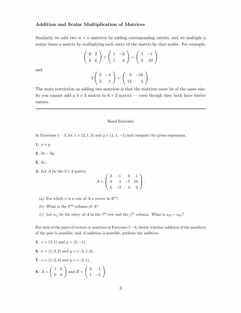
Addition and Scalar Multiplication of Matrices

Similarly, we add two m ! n matrices by adding corresponding entries, and we multiply ascalar times a matrix by multiplying each entry of the matrix by that scalar. For example,

'0 24 6

(

+

'1 "31 4

(

=

'1 "15 10

(

and

4

'2 "43 1

(

=

'8 "16

12 4

(

.

The main restriction on adding two matrices is that the matrices must be of the same size.So you cannot add a 4 ! 3 matrix to 6 ! 2 matrix — even though they both have twelveentries.

Hand Exercises

In Exercises 1 – 3, let x = (2, 1, 3) and y = (1, 1,!1) and compute the given expression.

1. x + y.

2. 2x! 3y.

3. 4x.

4. Let A be the 3" 4 matrix

A =

!

"#2 !1 0 13 4 !7 106 !3 4 2

$

%& .

(a) For which n is a row of A a vector in Rn?

(b) What is the 2nd column of A?

(c) Let aij be the entry of A in the ith row and the jth column. What is a23 ! a31?

For each of the pairs of vectors or matrices in Exercises 5 – 9, decide whether addition of the membersof the pair is possible; and, if addition is possible, perform the addition.

5. x = (2, 1) and y = (3,!1).

6. x = (1, 2, 2) and y = (!2, 1, 4).

7. x = (1, 2, 3) and y = (!2, 1).

8. A =

'1 30 4

(and B =

'2 11 !2

(.

3

9. A =

!

"#2 1 04 1 00 0 0

$

%& and B =

'2 11 !2

(.

In Exercises 10 – 11, let A =

'2 1!1 4

(and B =

'0 23 !1

(and compute the given expression.

10. 4A + B.

11. 2A! 3B.

1.2 MATLAB

We shall use MATLAB to compute addition and scalar multiplication of vectors in two and threedimensions. This will serve the purpose of introducing some basic MATLAB commands.

Entering Vectors and Vector Operations

Begin a MATLAB session. We now discuss how to enter a vector into MATLAB. The syntax isstraightforward; to enter the row vector x = (1, 2, 1) type1

x = [1 2 1]

and MATLAB responds with

x =

1 2 1

Next we show how easy it is to perform addition and scalar multiplication in MATLAB. Enterthe row vector y = (2,!1, 1) by typing

y = [2 -1 1]

and MATLAB responds with

y =

2 -1 11MATLAB has several useful line editing features. We point out two here:

(a) Horizontal arrow keys (!,") move the cursor one space without deleting a character.

(b) Vertical arrow keys (#, $) recall previous and next command lines.

4

To add the vectors x and y, type

x + y

and MATLAB responds with

ans =

3 1 2

This vector is easily checked to be the sum of the vectors x and y. Similarly, to perform a scalarmultiplication, type

2*x

which yields

ans =

2 4 2

MATLAB subtracts the vector y from the vector x in the natural way. Type

x - y

to obtain

ans =

-1 3 0

We mention two points concerning the operations that we have just performed in MATLAB.

(a) When entering a vector or a number, MATLAB automatically echoes what has been entered.This echoing can be suppressed by appending a semicolon to the line. For example, type

z = [-1 2 3];

and MATLAB responds with a new line awaiting a new command. To see the contents of thevector z just type z and MATLAB responds with

z =

-1 2 3

(b) MATLAB stores in a new vector the information obtained by algebraic manipulation. Type

a = 2*x - 3*y + 4*z;

5

Now type a to find

a =

-8 15 11

We see that MATLAB has created a new row vector a with the correct number of entries.

Note: In order to use the result of a calculation later in a MATLAB session, we need to namethe result of that calculation. To recall the calculation 2*x - 3*y + 4*z, we needed to name thatcalculation, which we did by typing a = 2*x - 3*y + 4*z. Then we were able to recall the resultjust by typing a.

We have seen that we enter a row n vector into MATLAB by surrounding a list of n numbersseparated by spaces with square brackets. For example, to enter the 5-vector w = (1, 3, 5, 7, 9) justtype

w = [1 3 5 7 9]

Note that the addition of two vectors is only defined when the vectors have the same number ofentries. Trying to add the 3-vector x with the 5-vector w by typing x + w in MATLAB yields thewarning:

??? Error using ==> +

Matrix dimensions must agree.

In MATLAB new rows are indicated by typing ;. For example, to enter the column vector

z =

!

"#!1

23

$

%& ,

just type:

z = [-1; 2; 3]

and MATLAB responds with

z =

-1

2

3

Note that MATLAB will not add a row vector and a column vector. Try typing x + z.

Individual entries of a vector can also be addressed. For instance, to display the first componentof z type z(1).

6

Entering Matrices

Matrices are entered into MATLAB row by row with rows separated either by semicolons or by linereturns. To enter the 2" 3 matrix

A =

'2 3 11 4 7

(,

just type

A = [2 3 1; 1 4 7]

MATLAB has very sophisticated methods for addressing the entries of a matrix. You can directlyaddress individual entries, individual rows, and individual columns. To display the entry in the 1st

row, 3rd column of A, type A(1,3). To display the 2nd column of A, type A(:,2); and to displaythe 1st row of A, type A(1,:). For example, to add the two rows of A and store them in the vectorx, just type

x = A(1,:) + A(2,:)

MATLAB has many operations involving matrices — these will be introduced later, as needed.

Computer Exercises

1. Enter the 3" 4 matrix

A =

!

"#1 2 5 7!1 2 1 !2

4 6 8 0

$

%& .

As usual, let aij denote the entry of A in the ith row and jth column. Use MATLAB to computethe following:

(a) a13 + a32.

(b) Three times the 3rd column of A.

(c) Twice the 2nd row of A minus the 3rd row.

(d) The sum of all of the columns of A.

2. Verify that MATLAB adds vectors only if they are of the same type, by typing

(a) x = [1 2], y = [2; 3] and x + y.

(b) x = [1 2], y = [2 3 1] and x + y.

In Exercises 3 – 4, let x = (1.2, 1.4,!2.45) and y = (!2.6, 1.1, 0.65) and use MATLAB to computethe given expression.

7

3. 3.27x! 7.4y.

4. 1.65x + 2.46y.

In Exercises 5 – 6, let

A =

'1.2 2.3 !0.50.7 !1.4 2.3

(and B =

'!2.9 1.23 1.6!2.2 1.67 0

(

and use MATLAB to compute the given expression.

5. !4.2A + 3.1B.

6. 2.67A! 1.1B.

1.3 Special Kinds of Matrices

There are many matrices that have special forms and hence have special names — which we nowlist.

• A square matrix is a matrix with the same number of rows and columns; that is, a squarematrix is an n" n matrix.

• A diagonal matrix is a square matrix whose only nonzero entries are along the main diagonal;that is, aij = 0 if i #= j. The following is a 3" 3 diagonal matrix

!

"#1 0 00 2 00 0 3

$

%& .

There is a shorthand in MATLAB for entering diagonal matrices. To enter this 3" 3 matrix,type diag([1 2 3]).

• The identity matrix is the diagonal matrix all of whose diagonal entries equal 1. The n " n

identity matrix is denoted by In. This identity matrix is entered in MATLAB by typingeye(n).

• A zero matrix is a matrix all of whose entries are 0. A zero matrix is denoted by 0. Thisnotation is ambiguous since there is a zero m " n matrix for every m and n. Nevertheless,this ambiguity rarely causes any di!culty. In MATLAB, to define an m " n matrix A whoseentries all equal 0, just type A = zeros(m,n). To define an n " n zero matrix B, type B =

zeros(n).

• The transpose of an m " n matrix A is the n "m matrix obtained from A by interchangingrows and columns. Thus the transpose of the 4" 2 matrix

!

"""#

2 1!1 2

3 !45 7

$

%%%&

8

is the 2" 4 matrix '2 !1 3 51 2 !4 7

(.

Suppose that you enter this 4" 2 matrix into MATLAB by typing

A = [2 1; -1 2; 3 -4; 5 7]

The transpose of a matrix A is denoted by At. To compute the transpose of A in MATLAB,just type A!.

• A symmetric matrix is a square matrix whose entries are symmetric about the main diagonal;that is aij = aji. Note that a symmetric matrix is a square matrix A for which At = A.

• An upper triangular matrix is a square matrix all of whose entries below the main diagonalare 0; that is, aij = 0 if i > j. A strictly upper triangular matrix is an upper triangular matrixwhose diagonal entries are also equal to 0. Similar definitions hold for lower triangular andstrictly lower triangular matrices. The following four 3 " 3 matrices are examples of uppertriangular, strictly upper triangular, lower triangular, and strictly lower triangular matrices:

!

"#1 2 30 2 40 0 6

$

%&

!

"#0 2 30 0 40 0 0

$

%&

!

"#7 0 05 2 0!4 1 !3

$

%&

!

"#0 0 05 0 0

10 1 0

$

%& .

• A square matrix A is block diagonal if

A =

!

""""#

B1 0 · · · 00 B2 · · · 0...

.... . .

...0 0 · · · Bk

$

%%%%&

where each Bj is itself a square matrix. An example of a 5 " 5 block diagonal matrix withone 2" 2 block and one 3" 3 block is:

!

""""""#

2 3 0 0 04 1 0 0 00 0 1 2 30 0 3 2 40 0 1 1 5

$

%%%%%%&.

Hand Exercises

In Exercises 1 – 5 decide whether or not the given matrix is symmetric.

1.

'2 11 5

(.

9

2.

'1 10 !5

(.

3. (3).

4.

!

"#3 44 30 1

$

%&.

5.

!

"#3 4 !14 3 1!1 1 10

$

%&.

In Exercises 6 – 10 decide which of the given matrices are upper triangular and which are strictlyupper triangular.

6.

'2 0!1 !2

(.

7.

'0 40 0

(.

8. (2).

9.

!

"#3 20 10 0

$

%&.

10.

!

"#0 2 !40 7 !20 0 0

$

%&.

A general 2 " 2 diagonal matrix has the form

'a 00 b

(. Thus the two unknown real numbers a

and b are needed to specify each 2" 2 diagonal matrix. In Exercises 11 – 16, how many unknownreal numbers are needed to specify each of the given matrices:

11. An upper triangular 2" 2 matrix?

12. A symmetric 2" 2 matrix?

13. An m" n matrix?

14. A diagonal n" n matrix?

15. An upper triangular n" n matrix? Hint: Recall the summation formula:

1 + 2 + · · ·+ k =k(k + 1)

2.

16. A symmetric n" n matrix?

10

In each of Exercises 17 – 19 determine whether the statement is True or False?

17. Every symmetric, upper triangular matrix is diagonal.

18. Every diagonal matrix is a multiple of the identity matrix.

19. Every block diagonal matrix is symmetric.

Computer Exercises

20. Use MATLAB to compute At when

A =

!

"#1 2 4 72 1 5 64 6 2 1

$

%& (1.3.1)

Use MATLAB to verify that (At)t = A by setting B=A’, C=B’, and checking that C = A.

21. Use MATLAB to compute At when A = (3) is a 1" 1 matrix.

1.4 The Geometry of Vector Operations

In this section we discuss the geometry of addition, scalar multiplication, and dot product of vectors.We also use MATLAB graphics to visualize these operations.

Geometry of Addition

MATLAB has an excellent graphics language that we shall use at various times to illustrate conceptsin both two and three dimensions. In order to make the connections between ideas and graphicsmore transparent, we will sometimes use previously developed MATLAB programs. We begin withsuch an example — the illustration of the parallelogram law for vector addition.

Suppose that x and y are two planar vectors. Think of these vectors as line segments from theorigin to the points x and y in R2. We use a program written by T.A. Bryan to visualize x + y. InMATLAB type2:

x = [1 2];

y = [-2 3];

addvec(x,y)

The vector x is displayed in blue, the vector y in green, and the vector x + y in red. Note that x + y

is just the diagonal of the parallelogram spanned by x and y. A black and white version of thisfigure is given in Figure 1.1.

2Note that all MATLAB commands are case sensitive — upper and lower case must be correct

11

−5 −4 −3 −2 −1 0 1 2 3 4 5

−5

−4

−3

−2

−1

0

1

2

3

4

5

x

y

x+y

Figure 1.1: Addition of two planar vectors.

The parallelogram law (the diagonal of the parallelogram spanned by x and y is x+y) is equallyvalid in three dimensions. Use MATLAB to verify this statement by typing:

x = [1 0 2];

y = [-1 4 1];

addvec3(x,y)

The parallelogram spanned by x and y in R3 is shown in cyan; the diagonal x + y is shown in blue.See Figure 1.2. To test your geometric intuition, make several choices of vectors x and y. Note thatone vertex of the parallelogram is always the origin.

−4−2

02

4

−4−2

02

40

0.5

1

1.5

2

2.5

3

y

0

x+y

x

Figure 1.2: Addition of two vectors in three dimensions.

Geometry of Scalar Multiplication

In all dimensions scalar multiplication just scales the length of the vector. To discuss this point weneed to define the length of a vector. View an n-vector x = (x1, . . . , xn) as a line segment from theorigin to the point x. Using the Pythagorean theorem, it can be shown that the length or norm of

12

this line segment is:||x|| =

)x2

1 + · · ·+ x2n.

MATLAB has the command norm for finding the length of a vector. Test this by entering the3-vector

x = [1 4 2];

Then type

norm(x)

MATLAB responds with:

ans =

4.5826

which is indeed approximately$

1 + 42 + 22 =$

21.

Now suppose r % R and x % Rn. A calculation shows that

||rx|| = |r|||x||. (1.4.1)

See Exercise 17. Note also that if r is positive, then the direction of rx is the same as that of x; whileif r is negative, then the direction of rx is opposite to the direction of x. The lengths of the vectors3x and !3x are each three times the length of x — but these vectors point in opposite directions.Scalar multiplication by the scalar 0 produces the 0 vector, the vector whose entries are all zero.

Dot Product and Angles

The dot product of two n-vectors x = (x1, . . . , xn) and y = (y1, . . . , yn) is an important operationon vectors. It is defined by:

x · y = x1y1 + · · ·+ xnyn. (1.4.2)

Note that x · x is just ||x||2, the length of x squared.

MATLAB also has a command for computing dot products of n-vectors. Type

x = [1 4 2];

y = [2 3 -1];

dot(x,y)

MATLAB responds with the dot product of x and y, namely,

13

ans =

12

One of the most important facts concerning dot products is the one that states

x · y = 0 if and only if x and y are perpendicular. (1.4.3)

Indeed, dot product also gives a way of numerically determining the angle between n-vectors. (Note:By convention, the angle between two vectors is the angle whose measure is between 0" and 180".)

Theorem 1.4.1. Let ! be the angle between two nonzero n-vectors x and y. Then

cos ! =x · y

||x||||y||. (1.4.4)

It follows that cos ! = 0 if and only if x · y = 0. Thus (1.4.3) is valid.

Proof: Theorem 1.4.1 is just a restatement of the law of cosines. Recall that the law of cosinesstates that

c2 = a2 + b2 ! 2ab cos !,

where a, b, c are the lengths of the sides of a triangle and ! is the interior angle opposite the side oflength c. In vector notation we can form a triangle two of whose sides are given by x and y in Rn.The third side is just x! y as x = y + (x! y), as in Figure 1.3.

x

y

x-y

θ

0

Figure 1.3: Triangle formed by vectors x and y with interior angle !.

It follows from the law of cosines that

||x! y||2 = ||x||2 + ||y||2 ! 2||x||||y|| cos!.

We claim that||x! y||2 = ||x||2 + ||y||2 ! 2x · y.

Assuming that the claim is valid, it follows that

x · y = ||x||||y|| cos!,

14

which proves the theorem. Finally, compute

||x! y||2 = (x1 ! y1)2 + · · ·+ (xn ! yn)2

= (x21 ! 2x1y1 + y2

1) + · · ·+ (x2n ! 2xnyn + y2

n)

= (x21 + · · ·+ x2

n) ! 2(x1y1 + · · ·+ xnyn) + (y21 + · · ·+ y2

n)

= ||x||2! 2x · y + ||y||2

to verify the claim.

Theorem 1.4.1 gives a numerically e!cient method for computing the angle between vectors x

and y. In MATLAB this computation proceeds by typing

theta = acos(dot(x,y)/(norm(x)*norm(y)))

where acos is the inverse cosine of a number. For example, using the 3-vectors x = (1, 4, 2) andy = (2, 3,!1) entered previously, MATLAB responds with

theta =

0.7956

Remember that this answer is in radians. To convert this answer to degrees, just multiply by 360and divide by 2":

360*theta / (2*pi)

to obtain the answer of 45.5847".

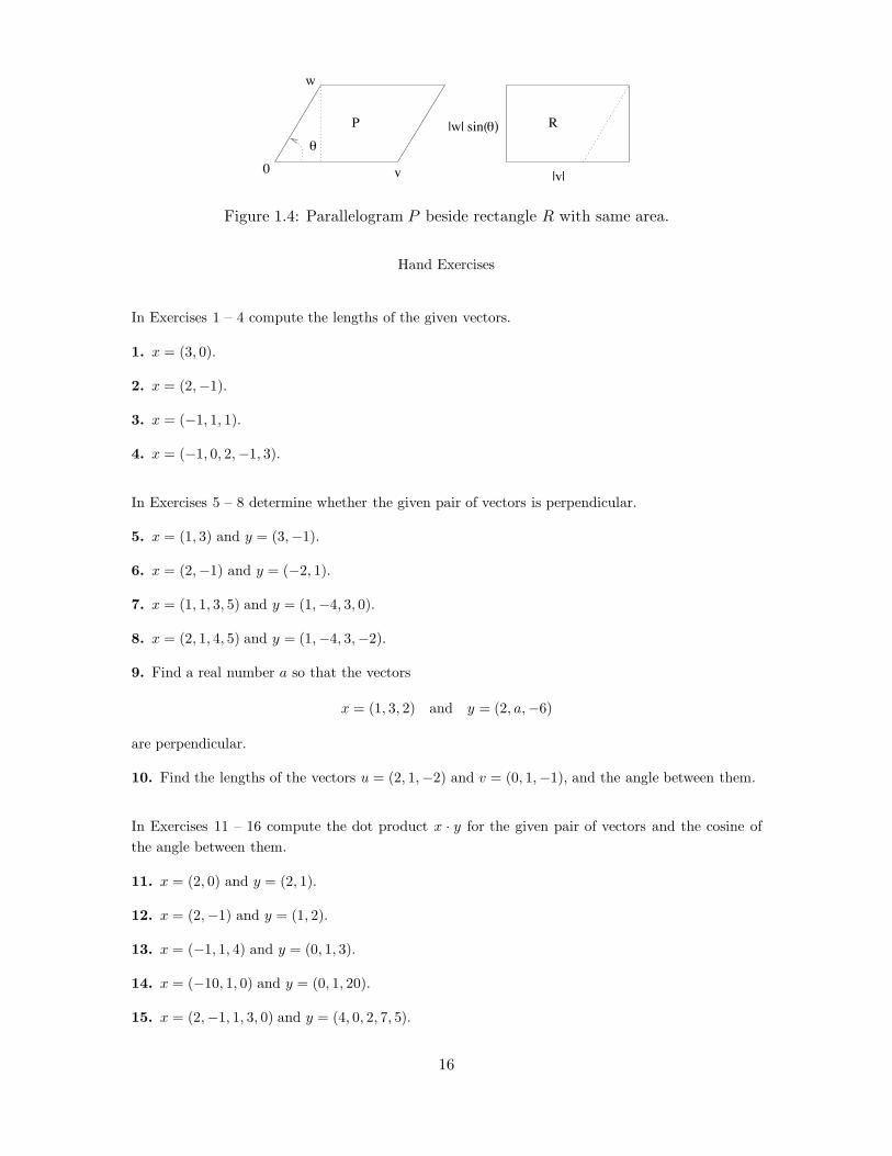
Area of Parallelograms

Let P be a parallelogram whose sides are the vectors v and w as in Figure 1.4. Let |P | denote thearea of P . As an application of dot products and (1.4.4), we calculate |P |. We claim that

|P |2 = ||v||2||w||2! (v ·w)2. (1.4.5)

We verify (1.4.5) as follows. Note that the area of P is the same as the area of the rectangle R alsopictured in Figure 1.4. The side lengths of R are: ||v|| and ||w|| sin! where ! is the angle between v

and w. A computation using (1.4.4) shows that

|R|2 = ||v||2||w||2 sin2 !

= ||v||2||w||2(1! cos2 !)

= ||v||2||w||2'

1!*

v · w||v||||w||

+2(

= ||v||2||w||2! (v · w)2,

which establishes (1.4.5).

15

R

0 v

w

|v|

θ

P |w| sin( θ)

Figure 1.4: Parallelogram P beside rectangle R with same area.

Hand Exercises

In Exercises 1 – 4 compute the lengths of the given vectors.

1. x = (3, 0).

2. x = (2,!1).

3. x = (!1, 1, 1).

4. x = (!1, 0, 2,!1, 3).

In Exercises 5 – 8 determine whether the given pair of vectors is perpendicular.

5. x = (1, 3) and y = (3,!1).

6. x = (2,!1) and y = (!2, 1).

7. x = (1, 1, 3, 5) and y = (1,!4, 3, 0).

8. x = (2, 1, 4, 5) and y = (1,!4, 3,!2).

9. Find a real number a so that the vectors

x = (1, 3, 2) and y = (2, a,!6)

are perpendicular.

10. Find the lengths of the vectors u = (2, 1,!2) and v = (0, 1,!1), and the angle between them.

In Exercises 11 – 16 compute the dot product x · y for the given pair of vectors and the cosine ofthe angle between them.

11. x = (2, 0) and y = (2, 1).

12. x = (2,!1) and y = (1, 2).

13. x = (!1, 1, 4) and y = (0, 1, 3).

14. x = (!10, 1, 0) and y = (0, 1, 20).

15. x = (2,!1, 1, 3, 0) and y = (4, 0, 2, 7, 5).

16

16. x = (5,!1, 4, 1, 0,0) and y = (!3, 0, 0, 1, 10,!5).

17. Using the definition of length, verify that formula (1.4.1) is valid.

Computer Exercises

18. Use addvec and addvec3 to add vectors in R2 and R3. More precisely, enter pairs of 2-vectorsx and y of your choosing into MATLAB, use addvec to compute x+y, and note the parallelogramformed by 0, x, y, x + y. Similarly, enter pairs of 3-vectors and use addvec3.

19. Determine the vector of length 1 that points in the same direction as the vector

x = (2, 13.5,!6.7,5.23).

20. Determine the vector of length 1 that points in the same direction as the vector

y = (2.1,!3.5, 1.5, 1.3,5.2).

In Exercises 21– 23 find the angle in degrees between the given pair of vectors.

21. x = (2, 1,!3, 4) and y = (1, 1,!5, 7).

22. x = (2.43, 10.2,!5.27,") and y = (!2.2, 0.33, 4,!1.7).

23. x = (1,!2, 2, 1, 2.1) and y = (!3.44, 1.2, 1.5,!2,!3.5).

In Exercises 24 – 25 let P be the parallelogram generated by the given vectors v and w in R3.Compute the area of that parallelogram.

24. v = (1, 5, 7) and w = (!2, 4, 13).

25. v = (2,!1, 1) and w = (!1, 4, 3).

17

Chapter 2

Solving Linear Equations

A linear equation in n unknowns, x1, x2, . . . , xn, is an equation of the form

a1x1 + a2x2 + · · ·+ anxn = b

where a1, a2, . . . , an and b are given numbers. The numbers a1, a2, . . . , an, are calledthe coe!cients of the equation. In particular, the equation

ax = b,

is a linear equation in one unknown;

ax + by = c,

is a linear equation in two unknowns (if a and b are real numbers and not both 0, thegraph of the equation is a straight line); and

ax + by + cz = d,

is a linear equation in three unknowns (if a, b and c are real numbers and not all 0,then the graph is a plane in 3-space).

Our main interest in this chapter is in solving systems of linear equations. This workprovides the basis for a general study of vectors and matrices. The algorithms that enableus to find solutions are themselves based on certain kinds of matrix manipulations. In thesealgorithms, matrices serve as a shorthand for calculation, rather than as a basis for a theory.We will see later that these matrix manipulations do lead to a rich theory of how to solvesystems of linear equations. But our first step is just to see how these equations are actuallysolved.

We begin with a discussion in Section 2.1 of how to write systems of linear equationsin terms of matrices. We also show by example how complicated writing down the answer

18

to such systems can be. In Section 2.2, we recall that solution sets to systems of linearequations in two and three variables are points, lines or planes.

The best known and probably the most e!cient method for solving systems of linearequations (especially with a moderate to large number of unknowns) is Gaussian elimination.The idea behind this method, which is introduced in Section 2.3, is to manipulate matricesby elementary row operations to reduced echelon form. It is then possible just to look atthe reduced echelon form matrix and to read o" the solutions to the linear system, if any.The process of reading o" the solutions is formalized in Section 2.4; see Theorem 2.4.6. Ourdiscussion of solving linear equations is presented with equations whose coe!cients are realnumbers — though most of our examples have just integer coe!cients. The methods workjust as well with complex numbers, and this generalization is discussed in Section 2.5.

Throughout this chapter, we alternately discuss the theory and show how calculationsthat are tedious when done by hand can easily be performed by computer using MATLAB.The chapter ends with a proof of the uniqueness of row echelon form (a topic of theoreticalimportance) in Section 2.6. This section is included mainly for completeness and need notbe covered on a first reading.

2.1 Systems of Linear Equations and Matrices

It is a simple exercise to solve the system of two equations

x + y = 7"x + 3y = 1

(2.1.1)

to find that x = 5 and y = 2. One way to solve system (2.1.1) is to add the two equations,obtaining

4y = 8;

hence y = 2. Substituting y = 2 into the 1st equation in (2.1.1) yields x = 5.

This system of equations can be solved in a more algorithmic fashion by solving the 1st

equation in (2.1.1) for x asx = 7 " y,

and substituting this answer into the 2nd equation in (2.1.1), to obtain

"(7 " y) + 3y = 1.

This equation simplifies to:4y = 8.

Now proceed as before.

19

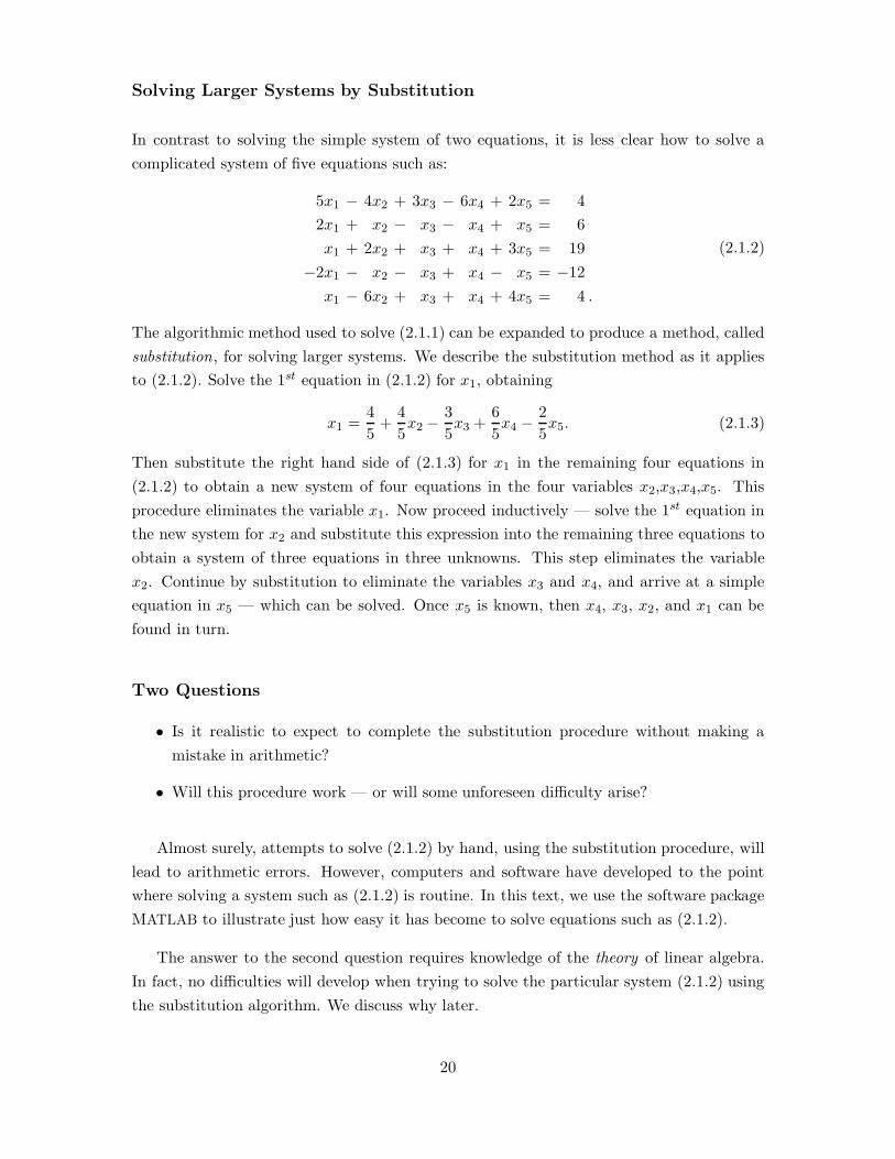
Solving Larger Systems by Substitution

In contrast to solving the simple system of two equations, it is less clear how to solve acomplicated system of five equations such as:

5x1 " 4x2 + 3x3 " 6x4 + 2x5 = 42x1 + x2 " x3 " x4 + x5 = 6x1 + 2x2 + x3 + x4 + 3x5 = 19

"2x1 " x2 " x3 + x4 " x5 = "12x1 " 6x2 + x3 + x4 + 4x5 = 4 .

(2.1.2)

The algorithmic method used to solve (2.1.1) can be expanded to produce a method, calledsubstitution, for solving larger systems. We describe the substitution method as it appliesto (2.1.2). Solve the 1st equation in (2.1.2) for x1, obtaining

x1 =45

+45x2 "

35x3 +

65x4 "

25x5. (2.1.3)

Then substitute the right hand side of (2.1.3) for x1 in the remaining four equations in(2.1.2) to obtain a new system of four equations in the four variables x2,x3,x4,x5. Thisprocedure eliminates the variable x1. Now proceed inductively — solve the 1st equation inthe new system for x2 and substitute this expression into the remaining three equations toobtain a system of three equations in three unknowns. This step eliminates the variablex2. Continue by substitution to eliminate the variables x3 and x4, and arrive at a simpleequation in x5 — which can be solved. Once x5 is known, then x4, x3, x2, and x1 can befound in turn.

Two Questions

• Is it realistic to expect to complete the substitution procedure without making amistake in arithmetic?

• Will this procedure work — or will some unforeseen di!culty arise?

Almost surely, attempts to solve (2.1.2) by hand, using the substitution procedure, willlead to arithmetic errors. However, computers and software have developed to the pointwhere solving a system such as (2.1.2) is routine. In this text, we use the software packageMATLAB to illustrate just how easy it has become to solve equations such as (2.1.2).

The answer to the second question requires knowledge of the theory of linear algebra.In fact, no di!culties will develop when trying to solve the particular system (2.1.2) usingthe substitution algorithm. We discuss why later.

20

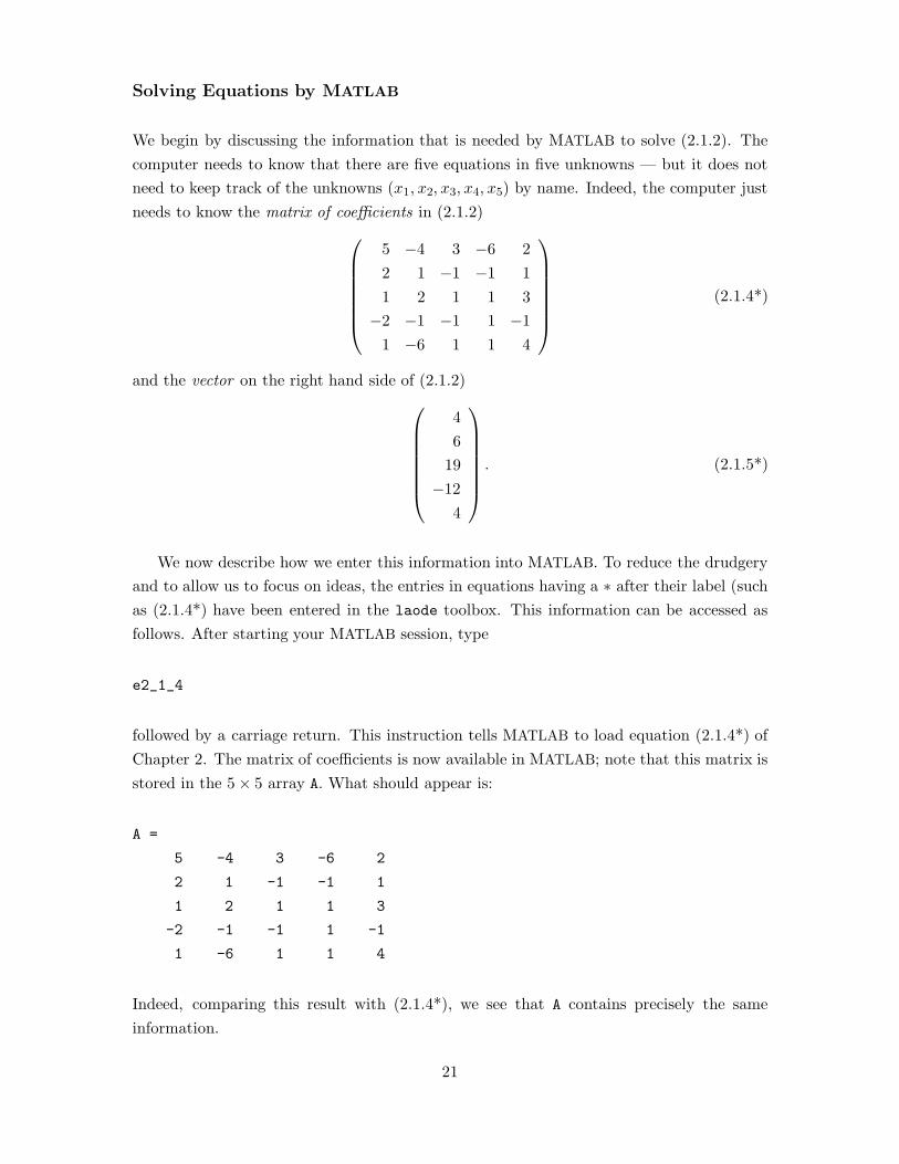
Solving Equations by MATLAB

We begin by discussing the information that is needed by MATLAB to solve (2.1.2). Thecomputer needs to know that there are five equations in five unknowns — but it does notneed to keep track of the unknowns (x1, x2, x3, x4, x5) by name. Indeed, the computer justneeds to know the matrix of coe!cients in (2.1.2)

!

""""""#

5 "4 3 "6 22 1 "1 "1 11 2 1 1 3

"2 "1 "1 1 "11 "6 1 1 4

$

%%%%%%&(2.1.4*)

and the vector on the right hand side of (2.1.2)!

""""""#

46

19"12

4

$

%%%%%%&. (2.1.5*)

We now describe how we enter this information into MATLAB. To reduce the drudgeryand to allow us to focus on ideas, the entries in equations having a # after their label (suchas (2.1.4*) have been entered in the laode toolbox. This information can be accessed asfollows. After starting your MATLAB session, type

e2_1_4

followed by a carriage return. This instruction tells MATLAB to load equation (2.1.4*) ofChapter 2. The matrix of coe!cients is now available in MATLAB; note that this matrix isstored in the 5 ! 5 array A. What should appear is:

A =

5 -4 3 -6 2

2 1 -1 -1 1

1 2 1 1 3

-2 -1 -1 1 -1

1 -6 1 1 4

Indeed, comparing this result with (2.1.4*), we see that A contains precisely the sameinformation.

21

Since the label (2.1.5*) is followed by a ‘#’, we can enter the vector in (2.1.5*) intoMATLAB by typing

e2_1_5

Note that the right hand side of (2.1.2) is stored in the vector b. MATLAB should haveresponded with

b =

4

6

19

-12

4

Now MATLAB has all the information it needs to solve the system of equations given in(2.1.2). To have MATLAB solve this system, type

x = A\b

to obtain

x =

5.0000

2.0000

3.0000

4.0000

1.0000

This answer is interpreted as follows: the five values of the unknowns x1, x2, x3, x4, x5

are stored in the vector x; that is,

x1 = 5, x2 = 2, x3 = 3, x4 = 4, x5 = 1. (2.1.6)

The reader may verify that (2.1.6) is indeed a solution of (2.1.2) by substituting the valuesin (2.1.6) into the equations in (2.1.2).

Changing Entries in MATLAB

MATLAB also permits access to single components of x. For instance, type

22

x(5)

and the 5th entry of x is displayed,

ans =

1.0000

We see that the component x(i) of x corresponds to the component xi of the vector x

where i = 1, 2, 3, 4, 5. Similarly, we can access the entries of the coe!cient matrix A. Forinstance, by typing

A(3,4)

MATLAB responds with

ans =

1

It is also possible to change an individual entry in either a vector or a matrix. Forexample, if we enter

A(3,4) = -2

we obtain a new matrix A which when displayed is:

A =

5 -4 3 -6 2

2 1 -1 -1 1

1 2 1 -2 3

-2 -1 -1 1 -1

1 -6 1 1 4

Thus the command A(3,4) = -2 changes the entry in the 3rd row, 4th column of A from 1to "2. In other words, we have now entered into MATLAB the information that is neededto solve the system of equations

5x1 " 4x2 + 3x3 " 6x4 + 2x5 = 42x1 + x2 " x3 " x4 + x5 = 6x1 + 2x2 + x3 " 2x4 + 3x5 = 19

"2x1 " x2 " x3 + x4 " x5 = "12x1 " 6x2 + x3 + x4 + 4x5 = 4 .

23

As expected, this change in the coe!cient matrix results in a change in the solution ofsystem (2.1.2), as well. Typing

x = A\b

now leads to the solution

x =

1.9455

3.0036

3.0000

1.7309

3.8364

that is displayed to an accuracy of four decimal places.

In the next step, change A as follows:

A(2,3) = 1

The new system of equations is:

5x1 " 4x2 + 3x3 " 6x4 + 2x5 = 42x1 + x2 + x3 " x4 + x5 = 6x1 + 2x2 + x3 " 2x4 + 3x5 = 19

"2x1 " x2 " x3 + x4 " x5 = "12x1 " 6x2 + x3 + x4 + 4x5 = 4 .

(2.1.7)

The command

x = A\b

now leads to the message

Warning: Matrix is singular to working precision.

x =

Inf

Inf

Inf

Inf

Inf

24

Obviously, something is wrong ; MATLAB cannot find a solution to this system of equations!Assuming that MATLAB is working correctly, we have shed light on one of our previousquestions: the method of substitution described by (2.1.3) need not always lead to a solution,even though the method does work for system (2.1.2). Why? As we will see, this is oneof the questions that is answered by the theory of linear algebra. In the case of (2.1.7), itis fairly easy to see what the di!culty is: the second and fourth equations have the formy = 6 and "y = "12, respectively.

Warning: The MATLAB command

x = A\b

may give an error message similar to the previous one. When this happens, one mustapproach the answer with caution.

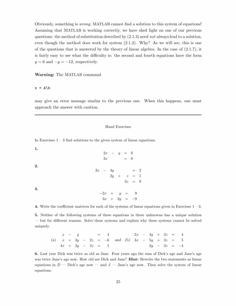
Hand Exercises

In Exercises 1 – 3 find solutions to the given system of linear equations.

1.2x ! y = 03x = 6

2.3x ! 4y = 2

2y + z = 13z = 9

3.!2x + y = 9

3x + 3y = !9

4. Write the coe!cient matrices for each of the systems of linear equations given in Exercises 1 – 3.

5. Neither of the following systems of three equations in three unknowns has a unique solution— but for di"erent reasons. Solve these systems and explain why these systems cannot be solveduniquely.

(a)x ! y = 4x + 3y ! 2z = !6

4x + 2y ! 3z = 1and (b)

2x ! 4y + 3z = 43x ! 5y + 3z = 5

2y ! 3z = !4

6. Last year Dick was twice as old as Jane. Four years ago the sum of Dick’s age and Jane’s agewas twice Jane’s age now. How old are Dick and Jane? Hint: Rewrite the two statements as linearequations in D — Dick’s age now — and J — Jane’s age now. Then solve the system of linearequations.

25

7. (a) Find a quadratic polynomial p(x) = ax2 + bx + c satisfying p(0) = 1, p(1) = 5, andp(!1) = !5.

(b) Prove that for every triple of real numbers L, M , and N , there is a quadratic polynomialsatisfying p(0) = L, p(1) = M , and p(!1) = N .

(c) Let x1, x2, x3 be three unequal real numbers and let A1, A2, A3 be three real numbers. Showthat finding a quadratic polynomial q(x) that satisfies q(xi) = Ai is equivalent to solving asystem of three linear equations.

Computer Exercises

8. Using MATLAB type the commands e2 1 8 and e2 1 9 to load the matrices:

A =

!

""""""""#

!5.6 0.4 !9.8 8.6 4.0 !3.4!9.1 6.6 !2.3 6.9 8.2 2.7

3.6 !9.3 !8.7 0.5 5.2 5.13.6 !8.9 !1.7 !8.2 !4.8 9.88.7 0.6 3.7 3.1 !9.1 !2.7!2.3 3.4 1.8 !1.7 4.7 !5.1

$

%%%%%%%%&

(2.1.8*)

and the vector

b =

!

""""""""#

9.74.55.13.0!8.5

2.6

$

%%%%%%%%&

(2.1.9*)

Solve the corresponding system of linear equations.

9. Matrices are entered in MATLAB as follows. To enter the 2" 3 matrix A, type A = [ -1 1 2;

4 1 2]. Enter this matrix into MATLAB; the displayed matrix should be

A =

-1 1 2

4 1 2

Now change the entry in the 2nd row, 1st column to !5.

10. Column vectors with n entries are viewed by MATLAB as n " 1 matrices. Enter the vector b

= [1; 2; -4]. Then change the 3rd entry in b to 13.

11. This problem illustrates some of the di"erent ways that MATLAB displays numbers using theformat long, the format short and the format rational commands.

Use MATLAB to solve the following system of equations

2x1 ! 4.5x2 + 3.1x3 = 4.2x1 + x2 + x3 = !5.1x1 ! 6.2x2 + x3 = 1.3 .

26

You may change the format of your answer in MATLAB. For example, to print your result with anaccuracy of 15 digits type format long and redisplay the answer. Similarly, to print your result asfractions type format rational and redisplay your answer.

12. Enter the following matrix and vector into MATLAB

A = [ 1 0 -1 ; 2 5 3 ; 5 -1 0];

b = [ 1; 1; -2];

and solve the corresponding system of linear equations by typing

x = A\b

Your answer should be

x =

-0.2000

1.0000

-1.2000

Find an integer for the entry in the 2nd row, 2nd column of A so that the solution

x = A\b

is not defined. Hint: The answer is an integer between !4 and 4.

13. The MATLAB command rand(m,n) defines matrices with random entries between 0 and 1. Forexample, the command A = rand(5,5) generates a random 5" 5 matrix, whereas the command b

= rand(5,1) generates a column vector with 5 random entries. Use these commands to constructseveral systems of linear equations and then solve them.

14. Suppose that the four substances S1, S2, S3, S4 contain the following percentages of vitaminsA, B, C and F by weight

Vitamin S1 S2 S3 S4

A 25% 19% 20% 3%B 2% 14% 2% 14%C 8% 4% 1% 0%F 25% 31% 25% 16%

Mix the substances S1, S2, S3 and S4 so that the resulting mixture contains precisely 3.85 grams ofvitamin A, 2.30 grams of vitamin B, 0.80 grams of vitamin C, and 5.95 grams of vitamin F. Howmany grams of each substance have to be contained in the mixture?

Discuss what happens if we require that the resulting mixture contains 2.00 grams of vitamin Binstead of 2.30 grams.

27

2.2 The Geometry of Low-Dimensional Solutions

In this section we discuss how to use MATLAB graphics to solve systems of linear equations in twoand three unknowns. We begin with two dimensions.

Linear Equations in Two Dimensions

The set of all solutions to the equation2x! y = 6 (2.2.1)

is a straight line in the xy plane; this line has slope 2 and y-intercept equal to !6. We can useMATLAB to plot the solutions to this equation — though some understanding of the way MATLABworks is needed.

The plot command in MATLAB plots a sequence of points in the plane, as follows. Let X andY be n vectors. Then

plot(X,Y)

will plot the points (X(1), Y (1)), (X(2), Y (2)), . . . , (X(n), Y (n)) in the xy-plane.

To plot points on the line (2.2.1) we need to enter the x-coordinates of the points we wish toplot. If we want to plot a hundred points, we would be facing a tedious task. MATLAB has acommand to simplify this task. Typing

x = linspace(-5,5,100);

produces a vector x with 100 entries with the 1st entry equal to !5, the last entry equal to 5, andthe remaining 98 entries equally spaced between !5 and 5. MATLAB has another command thatallows us to create a vector of points x. In this command we specify the distance between pointsrather than the number of points. That command is:

x = -5:0.1:5;

Producing x by either command is acceptable.

Typing

y = 2*x - 6;

produces a vector whose entries correspond to the y-coordinates of points on the line (2.2.1). Thentyping

plot(x,y)

28

produces the desired plot. It is useful to label the axes on this figure, which is accomplished bytyping

xlabel(’x’)

ylabel(’y’)

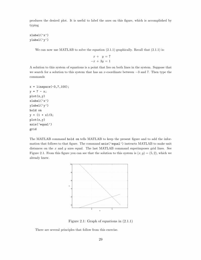
We can now use MATLAB to solve the equation (2.1.1) graphically. Recall that (2.1.1) is:

x + y = 7!x + 3y = 1

A solution to this system of equations is a point that lies on both lines in the system. Suppose thatwe search for a solution to this system that has an x-coordinate between !3 and 7. Then type thecommands

x = linspace(-3,7,100);

y = 7 - x;

plot(x,y)

xlabel(’x’)

ylabel(’y’)

hold on

y = (1 + x)/3;

plot(x,y)

axis(’equal’)

grid

The MATLAB command hold on tells MATLAB to keep the present figure and to add the infor-mation that follows to that figure. The command axis(’equal’) instructs MATLAB to make unitdistances on the x and y axes equal. The last MATLAB command superimposes grid lines. SeeFigure 2.1. From this figure you can see that the solution to this system is (x, y) = (5, 2), which wealready knew.

0 5

0

2

4

6

8

10

x

y

Figure 2.1: Graph of equations in (2.1.1)

There are several principles that follow from this exercise.

29

• Solutions to a single linear equation in two variables form a straight line.

• Solutions to two linear equations in two unknowns lie at the intersection of two straight linesin the plane.

It follows that the solution to two linear equations in two variables is a single point if the lines arenot parallel. If these lines are parallel and unequal, then there are no solutions, as there are nopoints of intersection. If the lines are parallel and equal, i.e., coincident, then there are infinitelymany solutions, namely the set of points on the (one) line. The latter two cases are illustrated below

x + 2y = 2!2x! 4y = !8

x + 2y = 22x + 4y = 4

-3 -2 -1 1 2 3

1

2

3

-3 -2 -1 1 2 3

1

2

Figure 2.2: Parallel and coincident lines

Linear Equations in Three Dimensions

We begin by observing that the set of all solutions to a linear equation in three variables forms aplane. More precisely, the solutions to the equation

ax + by + cz = d (2.2.2)

form a plane that is perpendicular to the vector (a, b, c) — assuming of course that the vector (a, b, c)is nonzero.

This fact is most easily proved using the dot product . Recall from Chapter 1 (1.4.2) that thedot product is defined by

X · Y = x1y1 + x2y2 + x3y3,

where X = (x1, x2, x3) and Y = (y1, y2, y3). We recall from Chapter 1 (1.4.3) the following importantfact concerning dot products:

X · Y = 0

if and only if the vectors X and Y are perpendicular.

Suppose that N = (a, b, c) #= 0. Consider the plane that is perpendicular to the normal vectorN and that contains the point X0. If the point X lies in that plane, then X !X0 is perpendicularto N ; that is,

(X !X0) · N = 0. (2.2.3)

30

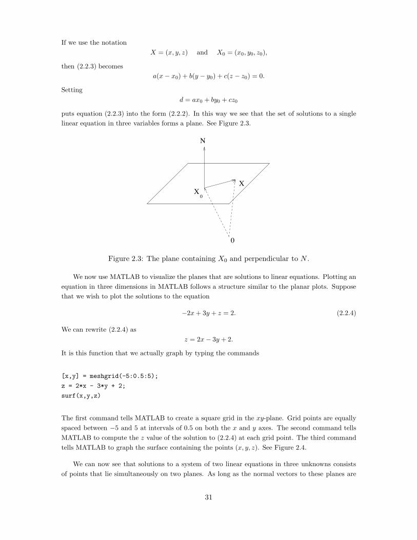
If we use the notationX = (x, y, z) and X0 = (x0, y0, z0),

then (2.2.3) becomesa(x! x0) + b(y ! y0) + c(z ! z0) = 0.

Settingd = ax0 + by0 + cz0

puts equation (2.2.3) into the form (2.2.2). In this way we see that the set of solutions to a singlelinear equation in three variables forms a plane. See Figure 2.3.

N

XX

0

0

Figure 2.3: The plane containing X0 and perpendicular to N .

We now use MATLAB to visualize the planes that are solutions to linear equations. Plotting anequation in three dimensions in MATLAB follows a structure similar to the planar plots. Supposethat we wish to plot the solutions to the equation

!2x + 3y + z = 2. (2.2.4)

We can rewrite (2.2.4) asz = 2x! 3y + 2.

It is this function that we actually graph by typing the commands

[x,y] = meshgrid(-5:0.5:5);

z = 2*x - 3*y + 2;

surf(x,y,z)

The first command tells MATLAB to create a square grid in the xy-plane. Grid points are equallyspaced between !5 and 5 at intervals of 0.5 on both the x and y axes. The second command tellsMATLAB to compute the z value of the solution to (2.2.4) at each grid point. The third commandtells MATLAB to graph the surface containing the points (x, y, z). See Figure 2.4.

We can now see that solutions to a system of two linear equations in three unknowns consistsof points that lie simultaneously on two planes. As long as the normal vectors to these planes are

31

−5

0

5

−5

0

5−30

−20

−10

0

10

20

30

Figure 2.4: Graph of (2.2.4).

not parallel, the intersection of the two planes will be a line in three dimensions. Indeed, considerthe equations

!2x + 3y + z = 2

2x! 3y + z = 0.

We can graph the solution using MATLAB , as follows. We continue from the previous graph bytyping

hold on

z = -2*x + 3*y;

surf(x,y,z)

The result, which illustrates that the intersection of two planes in R3 is generally a line, is shown inFigure 2.5.

−5

0

5

−5

0

5−30

−20

−10

0

10

20

30

Figure 2.5: Line of intersection of two planes.

We can now see geometrically that the solution to three simultaneous linear equations in threeunknowns will generally be a point — since generally three planes in three space intersect in a point.

32

To visualize this intersection, as shown in Figure 2.6, we extend the previous system of equations to

!2x + 3y + z = 2

2x! 3y + z = 0

!3x + 0.2y + z = 1.

Continuing in MATLAB type

hold on

z = 3*x - 0.2*y + 1;

surf(x,y,z)

−5

0

5

−5

0

5−30

−20

−10

0

10

20

30

Figure 2.6: Point of intersection of three planes.

Unfortunately, visualizing the point of intersection of these planes geometrically does not reallyhelp to get an accurate numerical value of the coordinates of this intersection point. However, wecan use MATLAB to solve this system accurately. Denote the 3 " 3 matrix of coe!cients by A,the vector of coe!cients on the right hand side by b, and the solution by x. Solve the system inMATLAB by typing

A = [ -2 3 1; 2 -3 1; -3 0.2 1];

b = [2; 0; 1];

x = A\b

The point of intersection of the three planes is at

x =

0.0233

0.3488

1.0000

Three planes in three dimensional space need not intersect in a single point. For example, iftwo of the planes are parallel they need not intersect at all. The normal vectors must point in

33

independent directions to guarantee that the intersection is a point. Understanding the notion ofindependence (it is more complicated than just not being parallel) is part of the subject of linearalgebra. MATLAB returns “Inf”, which we have seen previously, when these normal vectors are(approximately) dependent. For example, consider Exercise 6.

Plotting Nonlinear Functions in MATLAB

Suppose that we want to plot the graph of a nonlinear function of a single variable, such as

y = x2 ! 2x + 3 (2.2.5)

on the interval [!2, 5] using MATLAB. There is a di!culty: How do we enter the term x2? Forexample, suppose that we type

x = linspace(-2,5);

y = x*x - 2*x + 3;

Then MATLAB responds with

??? Error using ==> *

Inner matrix dimensions must agree.

The problem is that in MATLAB the variable x is a vector of 100 equally spaced points x(1), x(2),

..., x(100). What we really need is a vector consisting of entries x(1)*x(1), x(2)*x(2), ...,

x(100)*x(100). MATLAB has the facility to perform this operation automatically and the syntaxfor the operation is .* rather than *. So typing

x = linspace(-2,5);

y = x.*x - 2*x + 3;

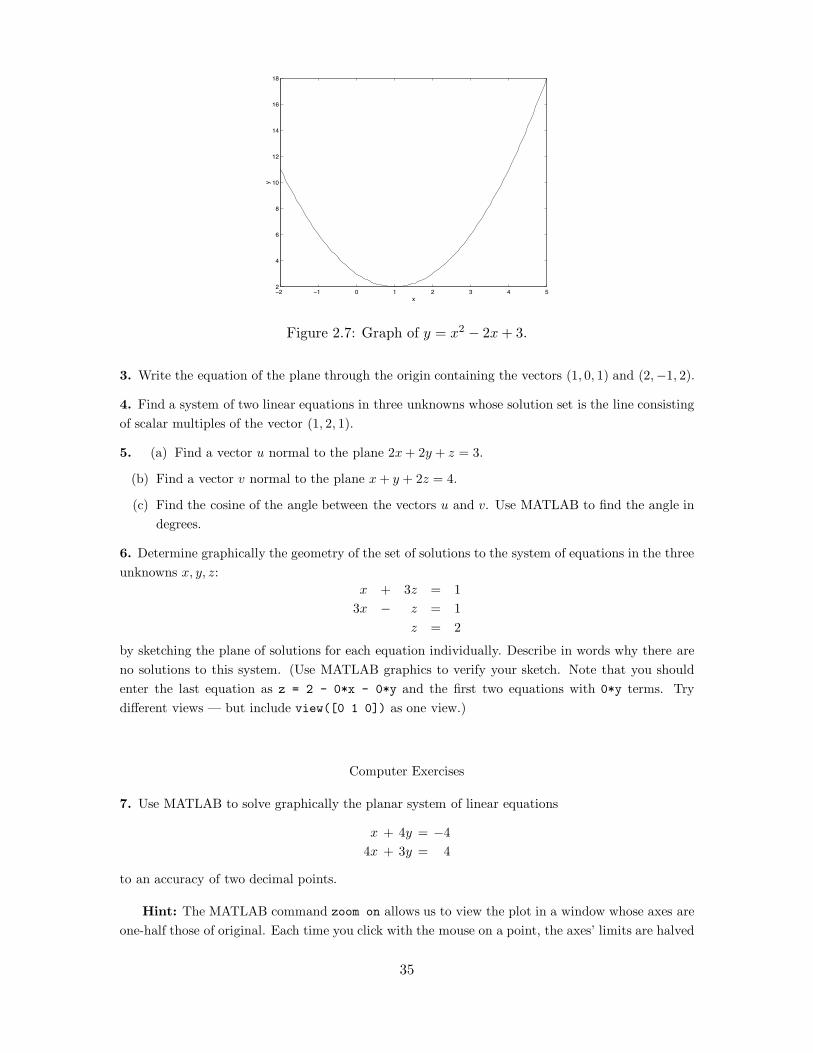
plot(x,y)

produces the graph of (2.2.5) in Figure 2.7. In a similar fashion, MATLAB has the ‘dot’ operationsof ./, .\, and .ˆ, as well as .*.

Hand Exercises

1. Find the equation for the plane perpendicular to the vector (2, 3, 1) and containing the point(!1,!2, 3).

2. Determine three systems of two linear equations in two unknowns so that the first system has aunique solution, the second system has an infinite number of solutions, and the third system has nosolutions.

34

−2 −1 0 1 2 3 4 52

4

6

8

10

12

14

16

18

x

y

Figure 2.7: Graph of y = x2 " 2x + 3.

3. Write the equation of the plane through the origin containing the vectors (1, 0, 1) and (2,!1, 2).

4. Find a system of two linear equations in three unknowns whose solution set is the line consistingof scalar multiples of the vector (1, 2, 1).

5. (a) Find a vector u normal to the plane 2x + 2y + z = 3.

(b) Find a vector v normal to the plane x + y + 2z = 4.

(c) Find the cosine of the angle between the vectors u and v. Use MATLAB to find the angle indegrees.

6. Determine graphically the geometry of the set of solutions to the system of equations in the threeunknowns x, y, z:

x + 3z = 13x ! z = 1

z = 2

by sketching the plane of solutions for each equation individually. Describe in words why there areno solutions to this system. (Use MATLAB graphics to verify your sketch. Note that you shouldenter the last equation as z = 2 - 0*x - 0*y and the first two equations with 0*y terms. Trydi"erent views — but include view([0 1 0]) as one view.)

Computer Exercises

7. Use MATLAB to solve graphically the planar system of linear equations

x + 4y = !44x + 3y = 4

to an accuracy of two decimal points.

Hint: The MATLAB command zoom on allows us to view the plot in a window whose axes areone-half those of original. Each time you click with the mouse on a point, the axes’ limits are halved

35

and centered at the designated point. Coupling zoom on with grid on allows you to determineapproximate numerical values for the intersection point.

8. Use MATLAB to solve graphically the planar system of linear equations

4.23x + 0.023y = !1.11.65x ! 2.81y = 1.63

to an accuracy of two decimal points.

9. Use MATLAB to find an approximate graphical solution to the three dimensional system of linearequations

3x ! 4y + 2z = !112x + 2y + z = 7!x + y ! 5z = 7.

Then use MATLAB to find an exact solution.

10. Use MATLAB to determine graphically the geometry of the set of solutions to the system ofequations:

x + 3y + 4z = 52x + y + z = 1!4x + 3y + 5z = 7.

Attempt to use MATLAB to find an exact solution to this system and discuss the implications ofyour calculations.

Hint: After setting up the graphics display in MATLAB, you can use the command view([0,1,0])

to get a better view of the solution point.

11. Use MATLAB to graph the function y = 2 ! x sin(x2 ! 1) on the interval [!2, 3]. How manyrelative maxima does this function have on this interval?

2.3 Gaussian Elimination

A general system of m linear equations in n unknowns has the form

a11x1 + a12x2 + · · · + a1nxn = b1

a21x1 + a22x2 + · · · + a2nxn = b2

......

......

am1x1 + am2x2 + · · · + amnxn = bm .

(2.3.1)

The entries aij and bi are constants. Our task is to find a method for solving (2.3.1) for the variablesx1, . . . , xn.

36

Easily Solved Equations

Some systems are easily solved. The system of three equations (m = 3) in three unknowns (n = 3)

x1 + 2x2 + 3x3 = 10x2 ! 1

5x3 = 75

x3 = 3(2.3.2)

is one example. The 3rd equation states that x3 = 3. Substituting this value into the 2nd equationallows us to solve the 2nd equation for x2 = 2. Finally, substituting x2 = 2 and x3 = 3 into the1st equation allows us to solve for x1 = !3. The process that we have just described is called backsubstitution.

Next, consider the system of two equations (m = 2) in three unknowns (n = 3):

x1 + 2x2 + 3x3 = 10x3 = 3 .

(2.3.3)

The 2nd equation in (2.3.3) states that x3 = 3. Substituting this value into the 1st equation leadsto the equation

x1 = 1! 2x2.

We have shown that every solution to (2.3.3) has the form (x1, x2, x3) = (1 ! 2x2, x2, 3) and thatevery vector (1! 2x2, x2, 3) is a solution of (2.3.3). Thus, there is an infinite number of solutions to(2.3.3), and these solutions can be parameterized by one number x2.

Equations Having No Solutions

Note that the system of equations

x1 ! x2 = 1

x1 ! x2 = 2

has no solutions.

Definition 2.3.1. A linear system of equations is inconsistent if the system has no solutions andconsistent if the system does have solutions.

As discussed in the previous section, (2.1.7) is an example of a linear system that MATLABcannot solve. In fact, that system is inconsistent — inspect the 2nd and 4th equations in (2.1.7).

Gaussian elimination is an algorithm for finding all solutions to a system of linear equations byreducing the given system to ones like (2.3.2) and (2.3.3), that are easily solved by back substitution.Consequently, Gaussian elimination can also be used to determine whether a system is consistent orinconsistent.

37

Elementary Equation Operations

There are three ways to change a system of equations without changing the set of solutions; Gaussianelimination is based on this observation. The three elementary operations are:

1. Swap two equations.

2. Multiply a single equation by a nonzero number.

3. Add a scalar multiple of one equation to another.

We begin with an example:

x1 + 2x2 + 3x3 = 10x1 + 2x2 + x3 = 4

2x1 + 9x2 + 5x3 = 27 .

(2.3.4)

Gaussian elimination works by eliminating variables from the equations in a fashion similar to thesubstitution method in the previous section. To begin, eliminate the variable x1 from all but the 1st

equation, as follows. Subtract the 1st equation from the 2nd, and subtract twice the 1st equationfrom the 3rd, obtaining:

x1 + 2x2 + 3x3 = 10!2x3 = !6

5x2 ! x3 = 7 .

(2.3.5)

Next, swap the 2nd and 3rd equations, so that the coe!cient of x2 in the new 2nd equation is nonzero.This yields

x1 + 2x2 + 3x3 = 105x2 ! x3 = 7

!2x3 = !6 .

(2.3.6)

Now, divide the 2nd equation by 5 and the 3rd equation by !2 to obtain a system of equationsidentical to our first example (2.3.2), which we solved by back substitution.

Augmented Matrices

The process of performing Gaussian elimination when the number of equations is greater than two orthree is painful. The computer, however, can help with the manipulations. We begin by introducingthe augmented matrix . The augmented matrix associated with (2.3.1) has m rows and n+1 columnsand is written as: !

""""#

a11 a12 · · · a1n b1

a21 a22 · · · a2n b2

......

......

am1 am2 · · · amn bm

$

%%%%&(2.3.7)

The augmented matrix contains all of the information that is needed to solve system (2.3.1).

38

Elementary Row Operations

The elementary operations used in Gaussian elimination can be interpreted as row operations onthe augmented matrix, as follows:

1. Swap two rows.

2. Multiply a single row by a nonzero number.

3. Add a scalar multiple of one row to another.

We claim that by using these elementary row operations intelligently, we can always solve a consistentlinear system — indeed, we can determine when a linear system is consistent or inconsistent. Theidea is to perform elementary row operations in such a way that the new augmented matrix has zeroentries below the diagonal.

We describe this process inductively. Begin with the 1st column. We assume for now that someentry in this column is nonzero. If a11 = 0, then swap two rows so that the number a11 is nonzero.Then divide the 1st row by a11 so that the leading entry in that row is 1. Now subtract ai1 timesthe 1st row from the ith row for each row i from 2 to m. The end result is that the 1st column hasa 1 in the 1st row and a 0 in every row below the 1st. The result is

!

""""#

1 & · · · &0 & · · · &...

......

...0 & · · · &

$

%%%%&.

Next we consider the 2nd column. We assume that some entry in that column below the 1st

row is nonzero. So, if necessary, we can swap two rows below the 1st row so that the entry a22 isnonzero. Then we divide the 2nd row by a22 so that its leading nonzero entry is 1. Then we subtractappropriate multiples of the 2nd row from each row below the 2nd so that all the entries in the 2nd

column below the 2nd row are 0. The result is!

""""#

1 & · · · &0 1 · · · &...

......

...0 0 · · · &

$

%%%%&.

Then we continue with the 3rd column. That’s the idea. However, does this process always workand what happens if all of the entries in a column are zero? Before answering these questions we doexperimentation with MATLAB.

Row Operations in MATLAB

In MATLAB the ith row of a matrix A is specified by A(i,:). Thus to replace the 5th row of amatrix A by twice itself, we need only type:

39

A(5,:) = 2*A(5,:)

In general, we can replace the ith row of the matrix A by c times itself by typing

A(i,:) = c*A(i,:)

Similarly, we can divide the ith row of the matrix A by the nonzero number c by typing

A(i,:) = A(i,:)/c

The third elementary row operation is performed similarly. Suppose we want to add c times theith row to the jth row, then we type

A(j,:) = A(j,:) + c*A(i,:)

For example, subtracting 3 times the 7th row from the 4th row of the matrix A is accomplished bytyping:

A(4,:) = A(4,:) - 3*A(7,:)

The first elementary row operation, swapping two rows, requires a di"erent kind of MATLABcommand. In MATLAB, the ith and jth rows of the matrix A are permuted by the command

A([i j],:) = A([j i],:)

So, to swap the 1st and 3rd rows of the matrix A, we type

A([1 3],:) = A([3 1],:)

Examples of Row Reduction in MATLAB

Let us see how the row operations can be used in MATLAB. As an example, we consider theaugmented matrix !

"""#

1 3 0 !1 !82 6 !4 4 41 0 !1 !9 !350 1 0 3 10

$

%%%&(2.3.8*)

We enter this information into MATLAB by typing

e2_3_8

40

which produces the result

A =

1 3 0 -1 -8

2 6 -4 4 4

1 0 -1 -9 -35

0 1 0 3 10

We now perform Gaussian elimination on A, and then solve the resulting system by back substi-tution. Gaussian elimination uses elementary row operations to set the entries that are in the lowerleft part of A to zero. These entries are indicated by numbers in the following matrix:

* * * * *

2 * * * *

1 0 * * *

0 1 0 * *

Gaussian elimination works inductively. Since the first entry in the matrix A is equal to 1, thefirst step in Gaussian elimination is to set to zero all entries in the 1st column below the 1st row.We begin by eliminating the 2 that is the first entry in the 2nd row of A. We replace the 2nd row bythe 2nd row minus twice the 1st row. To accomplish this elementary row operation, we type

A(2,:) = A(2,:) - 2*A(1,:)

and the result is

A =

1 3 0 -1 -8

0 0 -4 6 20

1 0 -1 -9 -35

0 1 0 3 10

In the next step, we eliminate the 1 from the entry in the 3rd row, 1st column of A. We do this bytyping

A(3,:) = A(3,:) - A(1,:)

which yields

A =

1 3 0 -1 -8

0 0 -4 6 20

0 -3 -1 -8 -27

0 1 0 3 10

41

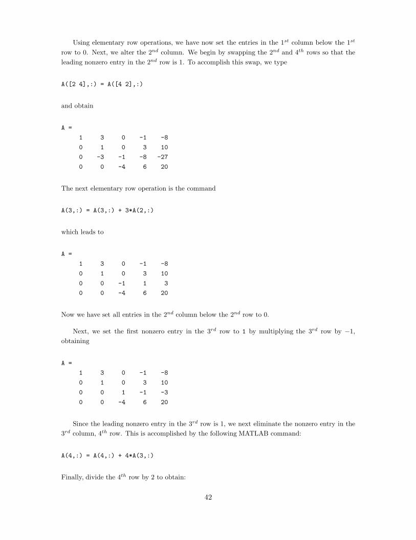
Using elementary row operations, we have now set the entries in the 1st column below the 1st

row to 0. Next, we alter the 2nd column. We begin by swapping the 2nd and 4th rows so that theleading nonzero entry in the 2nd row is 1. To accomplish this swap, we type

A([2 4],:) = A([4 2],:)

and obtain

A =

1 3 0 -1 -8

0 1 0 3 10

0 -3 -1 -8 -27

0 0 -4 6 20

The next elementary row operation is the command

A(3,:) = A(3,:) + 3*A(2,:)

which leads to

A =

1 3 0 -1 -8

0 1 0 3 10

0 0 -1 1 3

0 0 -4 6 20

Now we have set all entries in the 2nd column below the 2nd row to 0.

Next, we set the first nonzero entry in the 3rd row to 1 by multiplying the 3rd row by !1,obtaining

A =

1 3 0 -1 -8

0 1 0 3 10

0 0 1 -1 -3

0 0 -4 6 20

Since the leading nonzero entry in the 3rd row is 1, we next eliminate the nonzero entry in the3rd column, 4th row. This is accomplished by the following MATLAB command:

A(4,:) = A(4,:) + 4*A(3,:)

Finally, divide the 4th row by 2 to obtain:

42

A =

1 3 0 -1 -8

0 1 0 3 10

0 0 1 -1 -3

0 0 0 1 4

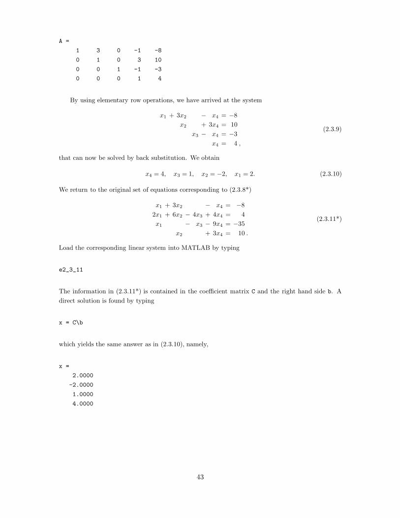
By using elementary row operations, we have arrived at the system

x1 + 3x2 ! x4 = !8x2 + 3x4 = 10

x3 ! x4 = !3x4 = 4 ,

(2.3.9)

that can now be solved by back substitution. We obtain

x4 = 4, x3 = 1, x2 = !2, x1 = 2. (2.3.10)

We return to the original set of equations corresponding to (2.3.8*)

x1 + 3x2 ! x4 = !82x1 + 6x2 ! 4x3 + 4x4 = 4x1 ! x3 ! 9x4 = !35

x2 + 3x4 = 10 .

(2.3.11*)

Load the corresponding linear system into MATLAB by typing

e2_3_11

The information in (2.3.11*) is contained in the coe!cient matrix C and the right hand side b. Adirect solution is found by typing

x = C\b

which yields the same answer as in (2.3.10), namely,

x =

2.0000

-2.0000

1.0000

4.0000

43

Introduction to Echelon Form

Next, we discuss how Gaussian elimination works in an example in which the number of rows andthe number of columns in the coe!cient matrix are unequal. We consider the augmented matrix

!

"""#

1 0 !2 3 4 0 10 1 2 4 0 !2 02 !1 !4 0 !2 8 !4!3 0 6 !8 !12 2 !2

$

%%%& (2.3.12*)

This information is entered into MATLAB by typing

e2_3_12

Again, the augmented matrix is denoted by A.

We begin by eliminating the 2 in the entry in the 3rd row, 1st column. To accomplish thecorresponding elementary row operation, we type

A(3,:) = A(3,:) - 2*A(1,:)

resulting in

A =

1 0 -2 3 4 0 1

0 1 2 4 0 -2 0

0 -1 0 -6 -10 8 -6

-3 0 6 -8 -12 2 -2

We proceed with

A(4,:) = A(4,:) + 3*A(1,:)

to create two more zeros in the 4th row. Finally, we eliminate the -1 in the 3rd row, 2nd column by

A(3,:) = A(3,:) + A(2,:)

to arrive at

A =

1 0 -2 3 4 0 1

0 1 2 4 0 -2 0

0 0 2 -2 -10 6 -6

0 0 0 1 0 2 1

44

Next we set the leading nonzero entry in the 3rd row to 1 by dividing the 3rd row by 2. That is, wetype

A(3,:) = A(3,:)/2

to obtain

A =

1 0 -2 3 4 0 1

0 1 2 4 0 -2 0

0 0 1 -1 -5 3 -3

0 0 0 1 0 2 1

We say that the matrix A is in (row) echelon form since the first nonzero entry in each row is a 1,each entry in a column below a leading 1 is 0, and the leading 1 moves to the right as you go downthe matrix. In row echelon form, the entries where leading 1’s occur are called pivots.

If we compare the structure of this matrix to the ones we have obtained previously, then we seethat here we have two columns too many. Indeed, we may solve these equations by back substitutionfor any choice of the variables x5 and x6.

The idea behind back substitution is to solve the last equation for the variable corresponding tothe first nonzero coe!cient. In this case, we use the 4th equation to solve for x4 in terms of x5 andx6, and then we substitute for x4 in the first three equations. This process can also be accomplishedby elementary row operations. Indeed, eliminating the variable x4 from the first three equations isthe same as using row operations to set the first three entries in the 4th column to 0. We can dothis by typing

A(3,:) = A(3,:) + A(4,:);

A(2,:) = A(2,:) - 4*A(4,:);

A(1,:) = A(1,:) - 3*A(4,:)

Remember: By typing semicolons after the first two rows, we have told MATLAB not to print theintermediate results. Since we have not typed a semicolon after the 3rd row, MATLAB outputs

A =

1 0 -2 0 4 -6 -2

0 1 2 0 0 -10 -4

0 0 1 0 -5 5 -2

0 0 0 1 0 2 1

We proceed with back substitution by eliminating the nonzero entries in the first two rows of the3rd column. To do this, type

45

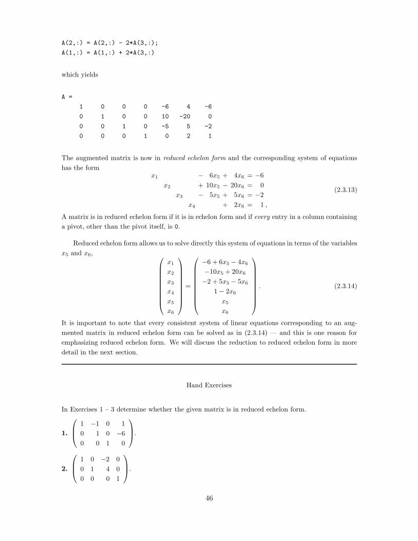
A(2,:) = A(2,:) - 2*A(3,:);

A(1,:) = A(1,:) + 2*A(3,:)

which yields

A =

1 0 0 0 -6 4 -6

0 1 0 0 10 -20 0

0 0 1 0 -5 5 -2

0 0 0 1 0 2 1

The augmented matrix is now in reduced echelon form and the corresponding system of equationshas the form

x1 ! 6x5 + 4x6 = !6x2 + 10x5 ! 20x6 = 0

x3 ! 5x5 + 5x6 = !2x4 + 2x6 = 1 ,

(2.3.13)

A matrix is in reduced echelon form if it is in echelon form and if every entry in a column containinga pivot, other than the pivot itself, is 0.

Reduced echelon form allows us to solve directly this system of equations in terms of the variablesx5 and x6, !

""""""""#

x1

x2

x3

x4

x5

x6

$

%%%%%%%%&

=

!

""""""""#

!6 + 6x5 ! 4x6

!10x5 + 20x6

!2 + 5x5 ! 5x6

1! 2x6

x5

x6

$

%%%%%%%%&

. (2.3.14)

It is important to note that every consistent system of linear equations corresponding to an aug-mented matrix in reduced echelon form can be solved as in (2.3.14) — and this is one reason foremphasizing reduced echelon form. We will discuss the reduction to reduced echelon form in moredetail in the next section.

Hand Exercises

In Exercises 1 – 3 determine whether the given matrix is in reduced echelon form.

1.

!

"#1 !1 0 10 1 0 !60 0 1 0

$

%&.

2.

!

"#1 0 !2 00 1 4 00 0 0 1

$

%&.

46

3.

!

"#0 1 0 30 0 2 10 0 0 0

$

%&.

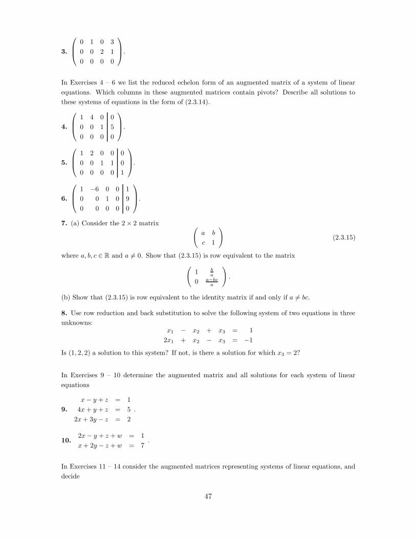
In Exercises 4 – 6 we list the reduced echelon form of an augmented matrix of a system of linearequations. Which columns in these augmented matrices contain pivots? Describe all solutions tothese systems of equations in the form of (2.3.14).

4.

!

"#1 4 0 00 0 1 50 0 0 0

$

%&.

5.

!

"#1 2 0 0 00 0 1 1 00 0 0 0 1

$

%&.

6.

!

"#1 !6 0 0 10 0 1 0 90 0 0 0 0

$

%&.

7. (a) Consider the 2" 2 matrix 'a b

c 1

((2.3.15)

where a, b, c % R and a #= 0. Show that (2.3.15) is row equivalent to the matrix'

1 ba

0 a#bca

(.

(b) Show that (2.3.15) is row equivalent to the identity matrix if and only if a #= bc.

8. Use row reduction and back substitution to solve the following system of two equations in threeunknowns:

x1 ! x2 + x3 = 12x1 + x2 ! x3 = !1

Is (1, 2, 2) a solution to this system? If not, is there a solution for which x3 = 2?

In Exercises 9 – 10 determine the augmented matrix and all solutions for each system of linearequations

9.x! y + z = 1

4x + y + z = 52x + 3y ! z = 2

.

10.2x! y + z + w = 1x + 2y ! z + w = 7

.

In Exercises 11 – 14 consider the augmented matrices representing systems of linear equations, anddecide

47

(a) if there are zero, one or infinitely many solutions, and

(b) if solutions are not unique, how many variables can be assigned arbitrary values.

11.

!

"#1 0 0 30 2 1 10 0 0 0

$

%&.

12.

!

"#1 2 0 0 30 1 1 0 10 0 0 0 2

$

%&.

13.

!

"#1 0 2 10 5 0 20 0 4 3

$

%&.

14.

!

"""#

1 0 2 0 32 3 6 1 160 3 2 1 100 0 0 0 0

$

%%%&.

A system of m equations in n unknowns is linear if it has the form (2.3.1); any other system ofequations is called nonlinear . In Exercises 15 – 19 decide whether each of the given systems ofequations is linear or nonlinear.

15.3x1 ! 2x2 + 14x3 ! 7x4 = 352x1 + 5x2 ! 3x3 + 12x4 = !1

16.3x1 + "x2 = 02x1 ! ex2 = 1

17.3x1x2 ! x2 = 10

2x1 ! x22 = !5

18.3x1 ! x2 = cos(12)2x1 ! x2 = !5

19.3x1 ! sin(x2) = 12

2x1 ! x3 = !5

Computer Exercises

In Exercises 20 – 22 use elementary row operations and MATLAB to put each of the given matricesinto row echelon form. Suppose that the matrix is the augmented matrix for a system of linearequations. Is the system consistent or inconsistent?

48

20. '2 1 14 2 3

(.

21. !

"#3 !4 0 20 2 3 13 1 4 5

$

%& .

22. !

"#!2 1 9 1

3 3 !4 21 4 5 5

$

%& .

Observation: In standard format MATLAB displays all nonzero real numbers with four decimalplaces while it displays zero as 0. An unfortunate consequence of this display is that when a matrixhas both zero and noninteger entries, the columns will not align — which is a nuisance. You canwork with rational numbers rather than decimal numbers by typing format rational. Then thecolumns will align.

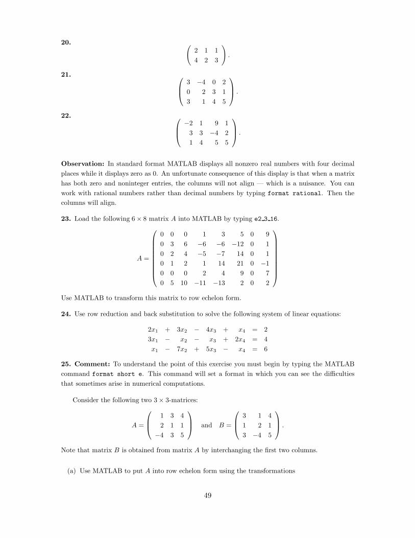
23. Load the following 6" 8 matrix A into MATLAB by typing e2 3 16.

A =

!

""""""""#

0 0 0 1 3 5 0 90 3 6 !6 !6 !12 0 10 2 4 !5 !7 14 0 10 1 2 1 14 21 0 !10 0 0 2 4 9 0 70 5 10 !11 !13 2 0 2

$

%%%%%%%%&

Use MATLAB to transform this matrix to row echelon form.

24. Use row reduction and back substitution to solve the following system of linear equations:

2x1 + 3x2 ! 4x3 + x4 = 23x1 ! x2 ! x3 + 2x4 = 4x1 ! 7x2 + 5x3 ! x4 = 6

25. Comment: To understand the point of this exercise you must begin by typing the MATLABcommand format short e. This command will set a format in which you can see the di!cultiesthat sometimes arise in numerical computations.

Consider the following two 3" 3-matrices:

A =

!

"#1 3 42 1 1!4 3 5

$

%& and B =

!

"#3 1 41 2 13 !4 5

$

%& .

Note that matrix B is obtained from matrix A by interchanging the first two columns.

(a) Use MATLAB to put A into row echelon form using the transformations

49

1. Subtract 2 times the 1st row from the 2nd.

2. Add 4 times the 1st row to the 3rd.

3. Divide the 2nd row by !5.

4. Subtract 15 times the 2nd row from the 3rd.

(b) Put B by hand into row echelon form using the transformations

1. Divide the 1st row by 3.

2. Subtract the 1st row from the 2nd.

3. Subtract 3 times the 1st row from the 3rd.

4. Multiply the 2nd row by 3/5.

5. Add 5 times the 2nd row to the 3rd.

(c) Use MATLAB to put B into row echelon form using the same transformations as in part (b).

(d) Discuss the outcome of the three transformations. Is there a di"erence in the results? Wouldyou expect to see a di"erence? Could the di"erence be crucial when solving a system of linearequations?

26. Find a cubic polynomialp(x) = ax3 + bx2 + cx + d

so that p(1) = 2, p(2) = 3, p!(!1) = !1, and p!(3) = 1.

2.4 Reduction to Echelon Form

In this section, we formalize our previous numerical experiments. We define more precisely thenotions of echelon form and reduced echelon form matrices, and we prove that every matrix can beput into reduced echelon form using a sequence of elementary row operations. Consequently, we willhave developed an algorithm for determining whether a system of linear equations is consistent orinconsistent, and for determining all solutions to a consistent system.

Definition 2.4.1. A matrix E is in (row) echelon form if two conditions hold.

(a) The first nonzero entry in each row of E is equal to 1. This leading entry 1 is called a pivot.

(b) A pivot in the (i+1)st row of E occurs in a column to the right of the column where the pivotin the ith row occurs.

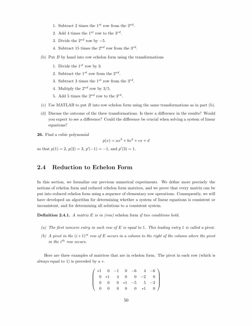
Here are three examples of matrices that are in echelon form. The pivot in each row (which isalways equal to 1) is preceded by a &.

!

"""#

&1 0 !1 0 !6 4 !60 &1 4 0 0 !2 00 0 0 &1 !5 5 !20 0 0 0 0 &1 0

$

%%%&

50

!

"""#

&1 0 !1 0 !60 &1 0 3 00 0 0 &1 !50 0 0 0 0

$

%%%&

!

"""#

0 &1 !1 14 !60 0 0 &1 150 0 0 0 00 0 0 0 0

$

%%%&

Here are three examples of matrices that are not in echelon form.!

"#0 0 1 151 !1 14 !60 0 0 0

$

%& and

!

"#1 !1 14 !60 0 3 150 0 0 0

$

%& and

!

"#1 !1 14 !60 0 0 00 0 1 15

$

%&

Definition 2.4.2. Two m " n matrices are row equivalent if one can be transformed to the otherby a sequence of elementary row operations.

Let A = (aij) be a matrix with m rows and n columns. We want to show that we can performrow operations on A so that the transformed matrix is in echelon form; that is, A is row equivalentto a matrix in echelon form. If A = 0, then we are finished. So we assume that some entry in A isnonzero and that the 1st column where that nonzero entry occurs is in the kth column. By swappingrows we can assume that a1k is nonzero. Next, divide the 1st row by a1k, thus setting a1k = 1. Now,using MATLAB notation, perform the row operations

A(i,:) = A(i,:) - A(i,k)*A(1,:)

for each i ' 2. This sequence of row operations leads to a matrix whose first nonzero column has a1 in the 1st row and a zero in each row below the 1st row.

Now we look for the next column that has a nonzero entry below the 1st row and call thatcolumn #. By construction # > k. We can swap rows so that the entry in the 2nd row, #th columnis nonzero. Then we divide the 2nd row by this nonzero element, so that the pivot in the 2nd rowis 1. Again we perform elementary row operations so that all entries below the 2nd row in the #th

column are set to 0. Now proceed inductively until we run out of nonzero rows.

This argument proves:

Proposition 2.4.3. Every matrix is row equivalent to a matrix in echelon form.

More importantly, the previous argument provides an algorithm for transforming matrices intoechelon form.

Reduction to Reduced Echelon Form

Definition 2.4.4. A matrix E is in reduced echelon form if

51

(a) E is in echelon form, and

(b) in every column of E having a pivot, every entry in that column other than the pivot is 0.

We can now prove

Theorem 2.4.5. Every matrix is row equivalent to a matrix in reduced echelon form.

Proof: Let A be a matrix. Proposition 2.4.3 states that we can transform A by elementary rowoperations to a matrix E in echelon form. Next we transform E into reduced echelon form by someadditional elementary row operations, as follows. Choose the pivot in the last nonzero row of E.Call that row #, and let k be the column where the pivot occurs. By adding multiples of the #th rowto the rows above, we can transform each entry in the kth column above the pivot to 0. Note thatnone of these row operations alters the matrix before the kth column. (Also note that this processis identical to the process of back substitution.)

Again we proceed inductively by choosing the pivot in the (#! 1)st row, which is 1, and zeroingout all entries above that pivot using elementary row operations.

Reduced Echelon Form in MATLAB

Preprogrammed into MATLAB is a routine to row reduce any matrix to reduced echelon form. Thecommand is rref. For example, recall the 4 " 7 matrix A in (2.3.12*) by typing e2 3 12. Put A

into reduced row echelon form by typing rref(A) and obtaining

ans =

1 0 0 0 -6 4 -6

0 1 0 0 10 -20 0

0 0 1 0 -5 5 -2

0 0 0 1 0 2 1

Compare the result with the system of equations (2.3.13).

Solutions to Systems of Linear Equations

Originally, we introduced elementary row operations as operations that do not change solutions tothe linear system. More precisely, we discussed how solutions to the original system are still solutionsto the transformed system and how no new solutions are introduced by elementary row operations.This argument is most easily seen by observing that

all elementary row operations are invertible

— they can be undone.

52

For example, swapping two rows is undone by just swapping these rows again. Similarly, multi-plying a row by a nonzero number c is undone by just dividing that same row by c. Finally, addingc times the jth row to the ith row is undone by subtracting c times the jth row from the ith row.

Thus, we can make several observations about solutions to linear systems. Let E be an aug-mented matrix corresponding to a system of linear equations having n variables. Since an augmentedmatrix is formed from the matrix of coe!cients by adding a column, we see that the augmentedmatrix has n + 1 columns.

Theorem 2.4.6. Suppose that E is an m " (n + 1) augmented matrix that is in reduced echelonform. Let # be the number of nonzero rows in E

(a) The system of linear equations corresponding to E is inconsistent if and only if the #th row inE has a pivot in the (n + 1)st column.

(b) If the linear system corresponding to E is consistent, then the set of all solutions is parame-terized by n! # parameters.

Proof: Suppose that the last nonzero row in E has its pivot in the (n + 1)st column. Then thecorresponding equation is:

0x1 + 0x2 + · · ·+ 0xn = 1,

which has no solutions. Thus the system is inconsistent.

Conversely, suppose that the last nonzero row has its pivot before the last column. Without lossof generality, we can renumber the columns — that is, we can renumber the variables xj — so thatthe pivot in the ith row occurs in the ith column, where 1 ( i ( #. Then the associated system oflinear equations has the form:

x1 + a1,!+1x!+1 + · · ·+ a1,nxn = b1

x2 + a2,!+1x!+1 + · · ·+ a2,nxn = b2

......

x! + a!,!+1x!+1 + · · ·+ a!,nxn = b!.

This system can be rewritten in the form:

x1 = b1 ! a1,!+1x!+1 ! · · ·! a1,nxn

x2 = b2 ! a2,!+1x!+1 ! · · ·! a2,nxn (2.4.1)...

...

x! = b! ! a!,!+1x!+1 ! · · ·! a!,nxn.

Thus, each choice of the n! # numbers x!+1, . . . , xn uniquely determines values of x1, . . . , x! sothat x1, . . . , xn is a solution to this system. In particular, the system is consistent, so (a) is proved;and the set of all solutions is parameterized by n! # numbers, so (b) is proved.

53

Two Examples Illustrating Theorem 2.4.6

The reduced echelon form matrix

E =

!

"#1 5 0 00 0 1 00 0 0 1

$

%&

is the augmented matrix of an inconsistent system of three equations in three unknowns.

The reduced echelon form matrix

E =

!

"#1 5 0 20 0 1 50 0 0 0

$

%&

is the augmented matrix of a consistent system of three equations in three unknowns x1, x2, x3. Forthis matrix n = 3 and # = 2. It follows from Theorem 2.4.6 that the solutions to this system arespecified by one parameter. Indeed, the solutions are

x1 = 2! 5x2

x3 = 5

and are specified by the one parameter x2.

Consequences of Theorem 2.4.6

It follows from Theorem 2.4.6 that linear systems of equations with fewer equations than unknownsand with zeros on the right hand side always have nonzero solutions. More precisely:

Corollary 2.4.7. Let A be an m " n matrix where m < n. Then the system of linear equationswhose augmented matrix is (A|0) has a nonzero solution.

Proof: Perform elementary row operations on the augmented matrix (A|0) to arrive at the reducedechelon form matrix (E|0). Since the zero vector is a solution, the associated system of equations isconsistent. Now the number of nonzero rows # in (E|0) is less than or equal to the number of rowsm in E. By assumption m < n and hence # < n. It follows from Theorem 2.4.6 that solutions to thelinear system are parametrized by n! # ' 1 parameters and that there are nonzero solutions.

Recall that two m " n matrices are row equivalent if one can be transformed to the other byelementary row operations.

Corollary 2.4.8. Let A be an n" n square matrix and let b be in Rn. Then A is row equivalent tothe identity matrix In if and only if the system of linear equations whose augmented matrix is (A|b)has a unique solution.

Proof: Suppose that A is row equivalent to In. Then, by using the same sequence of elementaryrow operations, it follows that the n " (n + 1) augmented matrix (A|b) is row equivalent to (In|c)

54

for some vector c % Rn. The system of linear equations that corresponds to (In|c) is:

x1 = c1

......

...xn = cn,

which transparently has the unique solution x = (c1, . . . , cn). Since elementary row operations donot change the solutions of the equations, the original augmented system (A|b) also has a uniquesolution.

Conversely, suppose that the system of linear equations associated to (A|b) has a unique so-lution. Suppose that (A|b) is row equivalent to a reduced echelon form matrix E. Suppose thatthe last nonzero row in E is the #th row. Since the system has a solution, it is consistent. HenceTheorem 2.4.6(b) implies that the solutions to the system corresponding to E are parameterized byn! # parameters. If # < n, then the solution is not unique. So # = n.

Next observe that since the system of linear equations is consistent, it follows from Theo-rem 2.4.6(a) that the pivot in the nth row must occur in a column before the (n + 1)st. It followsthat the reduced echelon matrix E = (In|c) for some c % Rn. Since (A|b) is row equivalent to (In|c),it follows, by using the same sequence of elementary row operations, that A is row equivalent toIn.

Uniqueness of Reduced Echelon Form and Rank

Abstractly, our discussion of reduced echelon form has one point remaining to be proved. We knowthat every matrix A can be transformed by elementary row operations to reduced echelon form.Suppose, however, that we use two di"erent sequences of elementary row operations to transform A

to two reduced echelon form matrices E1 and E2. Can E1 and E2 be di"erent? The answer is: No.

Theorem 2.4.9. For each matrix A, there is precisely one reduced echelon form matrix E that isrow equivalent to A.

The proof of Theorem 2.4.9 is given in Section 2.6. Since every matrix is row equivalent to aunique matrix in reduced echelon form, we can define the rank of a matrix as follows.

Definition 2.4.10. Let A be an m " n matrix that is row equivalent to a reduced echelon formmatrix E. Then the rank of A, denoted rank(A), is the number of nonzero rows in E.

We make three remarks concerning the rank of a matrix.

• An echelon form matrix is always row equivalent to a reduced echelon form matrix with thesame number of nonzero rows. Thus, to compute the rank of a matrix, we need only performelementary row operations until the matrix is in echelon form.

• The rank of any matrix is easily computed in MATLAB. Enter a matrix A and type rank(A).

• The number # in the statement of Theorem 2.4.6 is just the rank of E.

55

In particular, if the rank of the augmented matrix corresponding to a consistent system of linearequations in n unknowns has rank #, then the solutions to this system are parametrized by n ! #parameters.

Hand Exercises

In Exercises 1 – 2 row reduce the given matrix to reduced echelon form and determine the rank ofA.

1. A =

!

"#1 2 1 63 6 1 141 2 2 8

$

%&

2. B =

!

"#1 !2 33 !6 91 !8 2

$

%&

3. The augmented matrix of a consistent system of five equations in seven unknowns has rank equalto three. How many parameters are needed to specify all solutions?

4. The augmented matrix of a consistent system of nine equations in twelve unknowns has rankequal to five. How many parameters are needed to specify all solutions?

Computer Exercises

In Exercises 5 – 8, use rref on the given augmented matrices to determine whether the associ-ated system of linear equations is consistent or inconsistent. If the equations are consistent, thendetermine how many parameters are needed to enumerate all solutions.

5.

A =

!

"""#

2 1 3 !2 4 15 12 !1 3 5 1!4 !21 11 !12 2 123 59 !8 17 21 4

$

%%%& (2.4.2*)

6.

B =

!

"#2 4 6 !2 10 0 4 1 !12 4 0 1 2

$

%& (2.4.3*)

7.

C =

!

"#2 3 !1 48 11 !7 82 2 !4 !3

$

%& (2.4.4*)

56

8.

D =

!

"""#

2.3 4.66 !1.2 2.11 !20 0 1.33 0 1.44

4.6 9.32 !7.986 4.22 !10.0481.84 3.728 !5.216 1.688 !6.208

$

%%%&

In Exercises 9 – 11 compute the rank of the given matrix.

9.

'1 !2!3 6

(.

10.

!

"#2 1 0 1!1 3 2 4

5 !1 2 !2

$

%&.

11.

!

"""#

3 1 0!1 2 4

2 3 44 !1 !4

$

%%%&.

2.5 Linear Equations with Special Coe!cients

In this chapter we have shown how to use elementary row operations to solve systems of linearequations. We have assumed that each linear equation in the system has the form

aj1x1 + · · ·+ ajnxn = bj,

where the ajis and the bjs are real numbers. For simplicity, in our examples we have only chosenequations with integer coe!cients — such as:

2x1 ! 3x2 + 15x3 = !1.

Systems with Nonrational Coe!cients

In fact, a more general choice of coe!cients for a system of two equations might have been$

2x1 + 2"x2 = 22.4

3x1 + 36.2x2 = e. (2.5.1)

Suppose that we solve (2.5.1) by elementary row operations. In matrix form we have the aug-mented matrix ' $

2 2" 22.43 36.2 e

(.

57

Proceed with the following elementary row operations. Divide the 1st row by$

2 to obtain'

1 "$

2 11.2$

23 36.2 e

(.

Next, subtract 3 times the 1st row from the 2nd row to obtain:'

1 "$

2 11.2$

20 36.2! 3"

$2 e ! 33.6

$2

(.

Then divide the 2nd row by 36.2! 3"$

2, obtaining:'

1 "$

2 11.2$

20 1 e#33.6

$2

36.2#3"$

2

(.

Finally, multiply the 2nd row by "$

2 and subtract it from the 1st row to obtain:'

1 0 11.2$

2! "$

2 e#33.6$

236.2#3"

$2

0 1 e#33.6$

236.2#3"

$2

(.

So

x1 = 11.2$

2! "$

2e ! 33.6

$2

36.2! 3"$

2(2.5.2)

x2 =e ! 33.6

$2

36.2! 3"$

2

which is both hideous to look at and quite uninformative. It is, however, correct.

Both x1 and x2 are real numbers — they had to be because all of the manipulations involvedaddition, subtraction, multiplication, and division of real numbers — which yield real numbers.

If we wanted to use MATLAB to perform these calculations, we have to convert$

2, ", and e totheir decimal equivalents — at least up to a certain decimal place accuracy. This introduces errors— which for the moment we assume are small.

To enter A and b in MATLAB , type

A = [sqrt(2) 2*pi; 3 36.2];

b = [22.4; exp(1)];

Now type A to obtain:

A =

1.4142 6.2832

3.0000 36.2000

As its default display, MATLAB displays real numbers to four decimal place accuracy. Similarly,type b to obtain

58

b =

22.4000

2.7183

Next use MATLAB to solve this system by typing:

A\b

to obtain

ans =

24.5417

-1.9588

The reader may check that this answer agrees with the answer in (2.5.2) to MATLAB outputaccuracy by typing

x1 = 11.2*sqrt(2)-pi*sqrt(2)*(exp(1)-33.6*sqrt(2))/(36.2-3*pi*sqrt(2))

x2 = (exp(1)-33.6*sqrt(2))/(36.2-3*pi*sqrt(2))

to obtain

x1 =

24.5417

and

x2 =

-1.9588

More Accuracy

MATLAB can display numbers in machine precision (15 digits) rather than the standard four decimalplace accuracy. To change to this display, type

format long

Now solve the system of equations (2.5.1) again by typing

A\b

59

and obtaining

ans =

24.54169560069650

-1.95875151860858

Systems with Integers and Rational Numbers

Now suppose that all of the coe!cients in a system of linear equations are integers. When we add,subtract or multiply integers — we get integers. In general, however, when we divide an integer byan integer we get a rational number rather than an integer. Indeed, since elementary row operationsinvolve only the operations of addition, subtraction, multiplication and division, we see that if weperform elementary row operations on a matrix with integer entries, we will end up with a matrixwith rational numbers as entries.

MATLAB can display calculations using rational numbers rather than decimal numbers. Todisplay calculations using only rational numbers, type

format rational

For example, let

A =

!

"""#

2 2 1 01 3 !5 14 2 1 32 1 !1 4

$

%%%& (2.5.3*)

and let

b =

!

"""#

11!5

2

$

%%%& . (2.5.4*)

Enter A and b into MATLAB by typing

e2_5_3

e2_5_4

Solve the system by typing

A\b

to obtain

ans =

60

-357/41

309/41

137/41

156/41

To display the answer in standard decimal form, type

format

A\b

obtaining

ans =

-8.7073

7.5366

3.3415

3.8049

The same logic shows that if we begin with a system of equations whose coe!cients are rationalnumbers, we will obtain an answer consisting of rational numbers — since adding, subtracting,multiplying and dividing rational numbers yields rational numbers. More precisely:

Theorem 2.5.1. Let A be an n " n matrix that is row equivalent to In, and let b be an n vector.Suppose that all entries of A and b are rational numbers. Then there is a unique solution to the systemcorresponding to the augmented matrix (A|b) and this solution has rational numbers as entries.

Proof: Since A is row equivalent to In, Corollary 2.4.8 states that this linear system has a uniquesolution x. As we have just discussed, solutions are found using elementary row operations — hencethe entries of x are rational numbers.

Complex Numbers

In the previous parts of this section, we have discussed why solutions to linear systems whosecoe!cients are rational numbers must themselves have entries that are rational numbers. We nowdiscuss solving linear equations whose coe!cients are more general than real numbers; that is, whosecoe!cients are complex numbers.

First recall that addition, subtraction, multiplication and division of complex numbers yieldscomplex numbers. Suppose that

a = $+ i%

b = & + i'

61

where $, %, &, ' are real numbers and i =$!1. Then

a + b = ($+ &) + i(% + ')

a ! b = ($! &) + i(% ! ')

ab = ($& ! %') + i($' + %&)a

b=

$& + %'&2 + '2

+ i%& ! $'&2 + '2

MATLAB has been programmed to do arithmetic with complex numbers using exactly the sameinstructions as it uses to do arithmetic with real and rational numbers. For example, we can solvethe system of linear equations

(4! i)x1 + 2x2 = 3! i

2x1 + (4! 3i)x2 = 2 + i

in MATLAB by typing

A = [4-i 2; 2 4-3i];

b = [3-i; 2+i];

A\b

The solution to this system of equations is:

ans =

0.8457 - 0.1632i

-0.1098 + 0.2493i

Note: Care must be given when entering complex numbers into arrays in MATLAB. For example, if you

type

b = [3 -i; 2 +i]

then MATLAB will respond with the 2 % 2 matrix

b =

3.0000 0 - 1.0000i

2.0000 0 + 1.0000i

Typing either b = [3-i; 2+i] or b = [3 - i; 2 + i] will yield the desired 2 % 1 column vector.

All of the theorems concerning the existence and uniqueness of row echelon form — andfor solving systems of linear equations — work when the coe!cients of the linear systemare complex numbers as opposed to real numbers. In particular:

Theorem 2.5.2. If the coe!cients of a system of n linear equations in n unknowns arecomplex numbers and if the coe!cient matrix is row equivalent to In, then there is a uniquesolution to this system whose entries are complex numbers.

62

Complex Conjugation

Let a = " + i# be a complex number. Then the complex conjugate of a is defined to be

a = "" i#.

Let a = " + i# and c = $ + i% be complex numbers. Then we claim that

a + c = a + c

ac = a c(2.5.5)

To verify these statements, calculate

a + c = (" + $) + i(# + %) = (" + $)" i(# + %) = ("" i#) + ($ " i%) = a + c

and

ac = ("$ " #%) + i("% + #$) = ("$ " #%)" i("% + #$) = ("" i#)($ " i%) = a c.

Hand Exercises

1. Solve the system of equations

x1 ! ix2 = 1ix1 + 3x2 = !1

Check your answer using MATLAB.

Solve the systems of linear equations given in Exercises 2 – 3 and verify that the answers are rationalnumbers.

2.x1 + x2 ! 2x3 = 1x1 + x2 + x3 = 2x1 ! 7x2 + x3 = 3

3.x1 ! x2 = 1x1 + 3x2 = !1

Computer Exercises

In Exercises 4 – 6 use MATLAB to solve the given system of linear equations to four significantdecimal places.

63

4.0.1x1 +

$5x2 ! 2x3 = 1

!$

3x1 + "x2 ! 2.6x3 = 14.3x1 ! 7x2 + "

2x3 =$

2.

5.(4! i)x1 + (2 + 3i)x2 = !i

ix1 ! 4x2 = 2.2.

6.(2 + i)x1 + (

$2! 3i)x2 ! 10.66x3 = 4.23

14x1 !$

5ix2 + (10.2! i)x3 = 3! 1.6i

!4.276x1 + 2x2 ! (4! 2i)x3 =$

2i

.

Hint: When entering$

2i in MATLAB you must type sqrt(2)*i, even though when you enter 2i,you can just type 2i.

2.6 *Uniqueness of Reduced Echelon Form

In this section we prove Theorem 2.4.9, which states that every matrix is row equivalent to preciselyone reduced echelon form matrix.

Proof of Theorem 2.4.9: Suppose that E and F are two m"n reduced echelon matrices that arerow equivalent to A. Since elementary row operations are invertible, the two matrices E and F arerow equivalent. Thus, the systems of linear equations associated to the m" (n + 1) matrices (E|0)and (F |0) must have exactly the same set of solutions. It is the fact that the solution sets of thelinear equations associated to (E|0) and (F |0) are identical that allows us to prove that E = F .

Begin by renumbering the variables x1, . . . , xn so that the equations associated to (E|0) havethe form:

x1 = !a1,!+1x!+1 ! · · ·! a1,nxn

x2 = !a2,!+1x!+1 ! · · ·! a2,nxn

......

x! = !a!,!+1x!+1 ! · · ·! a!,nxn.

(2.6.1)

In this form, pivots of E occur in the columns 1, . . . , #. We begin by showing that the matrix F

also has pivots in columns 1, . . . , #. Moreover, there is a unique solution to these equations for everychoice of numbers x!+1, . . . , xn.

Suppose that the pivots of F do not occur in columns 1, . . . , #. Then there is a row in F whosefirst nonzero entry occurs in a column k > #. This row corresponds to an equation

xk = ck+1xk+1 + · · ·+ cnxn.

Now, consider solutions that satisfy

x!+1 = · · · = xk#1 = 0 and xk+1 = · · · = xn = 0.

64

In the equations associated to the matrix (E|0), there is a unique solution associated with everynumber xk; while in the equations associated to the matrix (F |0), xk must be zero to be a solution.This argument contradicts the fact that the (E|0) equations and the (F |0) equations have the samesolutions. So the pivots of F must also occur in columns 1, . . . , #, and the equations associated to F

must have the form:x1 = !a1,!+1x!+1 ! · · ·! a1,nxn

x2 = !a2,!+1x!+1 ! · · ·! a2,nxn

......

x! = !a!,!+1x!+1 ! · · ·! a!,nxn

(2.6.2)

where ai,j are scalars.

To complete this proof, we show that ai,j = ai,j. These equalities are verified as follows. Thereis just one solution to each system (2.6.1) and (2.6.2) of the form

x!+1 = 1, x!+2 = · · · = xn = 0.

These solutions are(!a1,!+1, . . . ,!a!,!+1, 1, 0, · · · , 0)

for (2.6.1) and(!a1,!+1, . . . ,!a!,!+1, 1, 0 · · · , 0)

for (2.6.2). It follows that aj,!+1 = aj,!+1 for j = 1, . . . , #. Complete this proof by repeating thisargument. Just inspect solutions of the form

x!+1 = 0, x!+2 = 1, x!+3 = · · · = xn = 0

throughx!+1 = · · · = xn#1 = 0, xn = 1.

65

Chapter 3

Matrices and Linearity

In this chapter we take the first step in abstracting vectors and matrices to mathematicalobjects that are more than just arrays of numbers. We begin the discussion in Section 3.1 byintroducing the multiplication of a matrix times a vector. Matrix multiplication simplifiesthe way in which we write systems of linear equations and is the way by which we viewmatrices as mappings. This latter point is discussed in Section 3.2.

The mappings that are produced by matrix multiplication are special and are calledlinear mappings. Some properties of linear maps are discussed in Section 3.3. One conse-quence of linearity is the principle of superposition that enables solutions to systems of linearequations to be built out of simpler solutions. This principle is discussed in Section 3.4.

In Section 3.5 we introduce multiplication of two matrices and discuss properties of thismultiplication in Section 3.6. Matrix multiplication is defined in terms of composition oflinear mappings which leads to an explicit formula for matrix multiplication. This dual roleof multiplication of two matrices — first by formula and second as composition — enablesus to solve linear equations in a conceptual way as well as in an algorithmic way. Theconceptual way of solving linear equations is through the use of matrix inverses (or inversemappings) which is described in Section 3.7. In this section we also present importantproperties of matrix inversion and a method of computation of matrix inverses. There is asimple formula for computing inverses of 2!2 matrices based on determinants. The chapterends with a discussion of determinants of 2 ! 2 matrices in Section 3.8.

66

3.1 Matrix Multiplication of Vectors

In Chapter 2 we discussed how matrices appear when solving systems of m linear equationsin n unknowns. Given the system

a11x1 + a12x2 + · · · + a1nxn = b1

a21x1 + a22x2 + · · · + a2nxn = b2...

......

...am1x1 + am2x2 + · · · + amnxn = bm ,

(3.1.1)

we saw that all relevant information is contained in the m ! n matrix of coe!cients

A =

!

""""#

a11 a12 · · · a1n

a21 a22 · · · a2n...

......

am1 am2 · · · amn

$

%%%%&

and the n vector

b =

!

""#

b1...

bn

$

%%& .

Matrices Times Vectors

We motivate multiplication of a matrix times a vector just as a notational advance thatsimplifies the presentation of the linear systems. It is, however, much more than that. Thisconcept of multiplication allows us to think of matrices as mappings and these mappingstell us much about the structure of solutions to linear systems. But first we discuss thenotational advantage.

Multiplying an m ! n matrix A times an n vector x produces an m vector, as follows:

Ax =

!

""#

a11 · · · a1n...

...am1 · · · amn

$

%%&

!

""#

x1...

xn

$

%%& =

!

""#

a11x1 + · · ·+ a1nxn...

am1x1 + · · ·+ amnxn

$

%%& . (3.1.2)

For example, when m = 2 and n = 3, then the product is a 2-vector

'a11 a12 a13

a21 a22 a23

(!

"#x1

x2

x3

$

%& =

'a11x1 + a12x2 + a13x3

a21x1 + a22x2 + a23x3

(

. (3.1.3)

67

As a specific example, compute

'2 3 "14 1 5

( !

"#2

"34

$

%& =

'2 · 2 + 3 · ("3) + ("1) · 44 · 2 + 1 · ("3) + 5 · 4

(

=

'"925

(

.

Using (3.1.2) we have a compact notation for writing systems of linear equations. Forexample, using a special instance of (3.1.3),

'2 3 "14 1 5

(!

"#x1

x2

x3

$

%& =

'2x1 + 3x2 " x3

4x1 + x2 + 5x3

(.

In this notation we can write the system of two linear equations in three unknowns

2x1 + 3x2 " x3 = 24x1 + x2 + 5x3 = "1

as the matrix equation

'2 3 "14 1 5

(!

"#x1

x2

x3

$

%& =

'2

"1

(.

Indeed, the general system of linear equations (3.1.1) can be written in matrix formusing matrix multiplication as

Ax = b

where A is the m ! n matrix of coe!cients, x is the n vector of unknowns, and b is the m

vector of constants on the right hand side of (3.1.1).

Matrices Times Vectors in MATLAB

We have already seen how to define matrices and vectors in MATLAB. Now we show howto multiply a matrix times a vector using MATLAB.

Load the matrix A

A =

!

""""""#

5 "4 3 "6 22 "4 "2 "1 11 2 1 "5 3

"2 "1 "2 1 "11 "6 1 1 4

$

%%%%%%&(3.1.4*)

68

and the vector x

x =

!

""""""#

"121

"13

$

%%%%%%&(3.1.5*)

into MATLAB by typing

e3_1_4

e3_1_5

The multiplication Ax can be performed by typing

b = A*x

and the result should be

b =

2

-8

18

-6

-1

We may verify this result by solving the system of linear equations Ax = b. Indeed if wetype

A\b

then we get the vector x back as the answer.

Hand Exercises

1. Let

A =

'2 1!1 4

(and x = (3, !2) .

Compute Ax.

69

2. Let

B =

'3 4 11 2 3

(and y =

!

"#25!2

$

%& .

Compute By.

In Exercises 3 – 6 decide whether or not the matrix vector product Ax can be computed; if it can,compute the product.

3. A =

'1 20 !5

(and x = (2, 2).

4. A =

'1 20 !5

(and x =

!

"#224

$

%&.

5. A =,

1 2 4-

and x =

!

"#!1

13

$

%&.

6. A = (5) and x = (1, 0).

7. Let

A =

!

""""#

a11 a12 · · · a1n

a21 a22 · · · a2n

......

...am1 am2 · · · amn

$

%%%%&and x =

!

""""#

x1

x2

...xn

$

%%%%&.

Denote the columns of the matrix A by

A1 =

!

""""#

a11

a21

...am1

$

%%%%&, A2 =

!

""""#

a12

a22

...am2

$

%%%%&, · · · An =

!

""""#

a1n

a2n

...amn

$

%%%%&.

Show that the matrix vector product Ax can be written as

Ax = x1A1 + x2A2 + · · ·+ xnAn,

where xjAj denotes scalar multiplication (see Chapter 1).

8. Let

C =

'1 12 !1

(and b = (1, 1) .

Find a 2-vector z such that Cz = b.

9. Write the system of linear equations

2x1 + 3x2 ! 2x3 = 4

6x1 ! 5x3 = 1

in the matrix form Ax = b.

70

10. Find all solutions to

!

"#1 3 !1 42 1 5 73 4 4 11

$

%&

!

"""#

x1

x2

x3

x4

$

%%%& =

!

"#141731

$

%& .

11. Let A be a 2" 2 matrix. Find A so that

A

'10

(=

'3!5

(

A

'01

(=

'14

(.

12. Let A be a 2" 2 matrix. Find A so that

A

'11

(=

'2!1

(

A

'1!1

(=

'43

(.

13. Is there an upper triangular 2" 2 matrix A such that

A (1, 0) = (1, 2)? (3.1.6)

Is there a symmetric 2" 2 matrix A satisfying (3.1.6)?

Computer Exercises

In Exercises 14 – 15 use MATLAB to compute b = Ax for the given A and x.

14.

A =

!

""""""#

!0.2 !1.8 3.9 !6 !1.66.3 8 3 2.5 5.1!0.8 !9.9 9.7 4.7 5.9!0.9 !4.1 1.1 !2.5 8.4!1 !9 !2 !9.8 6.9

$

%%%%%%&and x =

!

""""""#

!2.62.44.6!6.1

8.1

$

%%%%%%&. (3.1.7*)

15.

A =

!

""""""""""#

14 !22 !26 !2 !77 100 !9026 25 !15 !63 33 92 14!53 40 19 40 !27 !88 40

10 !21 13 97 !72 !28 9286 !17 43 61 13 10 50!33 31 2 41 65 !48 48

31 68 55 !3 35 19 !14

$

%%%%%%%%%%&

and x =

!

""""""""""#

2.76.1!8.3

8.98.3

2!4.9

$

%%%%%%%%%%&

. (3.1.8*)

71

16. Let

A =

!

"#2 4 !11 3 2!1 !2 5

$

%& and b =

!

"#214

$

%& . (3.1.9*)

Find a 3-vector x such that Ax = b.

17. Let

A =

!

"#1.3 !4.15 !1.21.6 !1.2 2.4!2.5 2.35 5.09

$

%& and b =

!

"#1.12!2.14.36

$

%& . (3.1.10*)

Find a 3-vector x such that Ax = b.

18. Let A be a 3" 3 matrix. Find A so that

A

!

"#2!1

1

$

%& =

!

"#11!1

$

%&

A

!

"#1!1

0

$

%& =

!

"#!1!2

1

$

%&

A

!

"#024

$

%& =

!

"#511

$

%& .

Hint: Rewrite these three conditions as a system of linear equations in the nine entries of A. Thensolve this system using MATLAB. (Then pray that there is an easier way.)

3.2 Matrix Mappings

Having illustrated the notational advantage of using matrices and matrix multiplication, we nowbegin to discuss why there is also a conceptual advantage to matrix multiplication, a conceptualadvantage that will help us to understand how systems of linear equations and linear di"erentialequations may be solved.

Matrix multiplication allows us to view m " n matrices as mappings from Rn to Rm. Let A bean m" n matrix and let x be an n vector. Then

x )* Ax

defines a mapping from Rn to Rm.

The simplest example of a matrix mapping is given by 1" 1 matrices. Matrix mappings definedfrom R* R are

x )* ax

where a is a real number. Note that the graph of this function is just a straight line through theorigin (with slope a). From this example we see that matrix mappings are very special mappings

72

indeed. In higher dimensions, matrix mappings provide a richer set of mappings; we explore hereplanar mappings — mappings of the plane into itself — using MATLAB graphics and the programmap.

The simplest planar matrix mappings are the dilatations. Let A = cI2 where c > 0 is a scalar.When c < 1 vectors are contracted by a factor of c and and these mappings are examples ofcontractions. When c > 1 vectors are stretched or expanded by a factor of c and these dilatationsare examples of expansions. We now explore some more complicated planar matrix mappings.

The next planar motions that we study are those given by the matrices

A =

'( 00 µ

(.

Here the matrix mapping is given by (x, y) )* ((x, µy); that is, a mapping that independentlystretches and/or contracts the x and y coordinates. Even these simple looking mappings can moveobjects in the plane in a somewhat complicated fashion.

The Program Map

We can use MATLAB to explore planar matrix mappings in an e!cient way using the program map.In MATLAB type the command

map

and a menu appears labeled MAP Setup. The 2" 2 matrix'

0 !11 0

(

has been pre-entered. Click on the Proceed button. A window entitled MAP Display appears. Clickon Icons and click on an icon — say Dog. Then click in the MAP Display window and a blue ‘Dog’will appear in that window. Now click on the Map button and a new version of the Dog will appearin yellow — but the yellow Dog is rotated about the origin counterclockwise by 90" from the bluedog. Indeed, this matrix A just rotates the plane counterclockwise by 90". To verify this statementjust click on Map again and see that the yellow dog rotates 90" counterclockwise into the magentadog. Of course, the magenta dog is just rotated 180" from the original blue dog. Clicking on Map

again produces a fourth dog — this one in cyan. Finally one more click on the map button willrotate the cyan dog into a red dog that exactly covers the original blue dog.

Choose another icon from the Icons menu; a blue version of this icon appears in the MAP Display

window. Now click on Map to see that your chosen icon is just rotated counterclockwise by 90".

Other matrices will produce di"erent motions of the plane. You may either type the entries ofa matrix in the Map Setup window and click on the Proceed button or recall one of the pre-assignedmatrices listed in the menu obtained by clicking on Gallery. For example, clicking on the Contracting

73

rotation button enters the matrix '0.3 !0.80.8 0.3

(

This matrix rotates the plane through an angle of approximately 69.4" counterclockwise and con-tracts the plane by a factor of approximately 0.85. Now click on Dog in the Icons menu to bringup the blue dog again. Repeated clicking on map rotates and contracts the dog so that dogs in acycling set of colors slowly converge towards the origin in a spiral of dogs.

Rotations

Rotating the plane counterclockwise through an angle ! is a motion given by a matrix mapping. Weshow that the matrix that performs this rotation is:

R# =

'cos ! ! sin !sin ! cos !

(. (3.2.1)

To verify that R# rotates the plane counterclockwise through angle !, let v$ be the unit vector whoseangle from the horizontal is ); that is, v$ = (cos), sin)). We can write every vector in R2 as rv$for some number r ' 0. Using the trigonometric identities for the cosine and sine of the sum of twoangles, we have:

R#(rv$) =

'cos ! ! sin !sin ! cos !

((r cos), r sin))

= (r cos ! cos) ! r sin ! sin), r sin ! cos) + r cos ! sin))

= r (cos(! + )), sin(! + )))

= rv$+#.

This calculation shows that R# rotates every vector in the plane counterclockwise through angle !.

It follows from (3.2.1) that R180! = !I2. So rotating a vector in the plane by 180" is the sameas reflecting the vector through the origin. It also follows that the movement associated with thelinear map x )* !cx where c > 0 may be thought of as a dilatation (x )* cx) followed by rotationthrough 180" (x )* !x).

We claim that combining dilatations with general rotations produces spirals. Consider the matrix

S =

'c cos ! !c sin !c sin ! c cos !

(= cR#

where c < 1. Then a calculation similar to the previous one shows that

S(rv$) = c(rv$+#).

So S rotates vectors in the plane while contracting them by the factor c. Thus, multiplying a vectorrepeatedly by S spirals that vector into the origin. The example that we just considered while usingmap is '

0.3 !0.80.8 0.3

(+=

'0.85 cos(69.4") !0.85 sin(69.4")0.85 sin(69.4") 0.85 cos(69.4")

(,

which has the general form of S.

74

A Notation for Matrix Mappings

We reinforce the idea that matrices are mappings by introducing a notation for the mapping asso-ciated with an m " n matrix A. Define

LA : Rn * Rm

byLA(x) = Ax,

for every x % Rn.

There are two special matrices: the m"n zero matrix O all of whose entries are 0 and the n"n

identity matrix In whose diagonal entries are 1 and whose o" diagonal entries are 0. For instance,

I3 =

!

"#1 0 00 1 00 0 1

$

%& .

The mappings associated with these special matrices are also special. Let x be an n vector.Then

Ox = 0, (3.2.2)

where the 0 on the right hand side of (3.2.2) is the m vector all of whose entries are 0. The mappingLO is the zero mapping — the mapping that maps every vector x to 0.

Similarly,Inx = x

for every vector x. It follows thatLIn(x) = x

is the identity mapping , since it maps every element to itself. It is for this reason that the matrixIn is called the n" n identity matrix .

Hand Exercises

In Exercises 1 – 3 find a nonzero vector that is mapped to the origin by the given matrix.

1. A =

'0 10 !2

(.

2. B =

'1 2!2 !4

(.

3. C =

'3 !1!6 2

(.

75

4. What 2" 2 matrix rotates the plane about the origin counterclockwise by 30"?

5. What 2" 2 matrix rotates the plane clockwise by 45"?

6. What 2" 2 matrix rotates the plane clockwise by 90" while dilating it by a factor of 2?

7. Find a 2" 2 matrix that reflects vectors in the (x, y) plane across the x axis.

8. Find a 2" 2 matrix that reflects vectors in the (x, y) plane across the y axis.

9. Find a 2" 2 matrix that reflects vectors in the (x, y) plane across the line x = y.

10. The matrix

A =

'1 K

0 1

(

is a shear. Describe the action of A on the plane for di"erent values of K.

11. Determine a rotation matrix that maps the vectors (3, 4) and (1,!2) onto the vectors (!4, 3)and (2, 1) respectively.

12. Find a 2"3 matrix P that projects three dimensional xyz space onto the xy plane. Hint: Sucha matrix will satisfy

P

!

"#00z

$

%& = (0, 0) and P

!

"#x

y

0

$

%& = (x, y) .

13. Show that every matrix of the form

'a !b

b a

(corresponds to rotating the plane through the

angle ! followed by a dilatation cI2 where

c =.

a2 + b2

cos ! =a

c

sin ! =b

c.

14. Using Exercise 13 observe that the matrix

'3 4!4 3

(rotates the plane counterclockwise

through an angle ! and then dilates the planes by a factor of c. Find ! and c. Use map to verifyyour results.

Computer Exercises

In Exercises 15 – 17 use map to find vectors that are stretched and/or contracted to a multiple ofthemselves by the given linear mapping. Hint: Choose a vector in the MAP Display window andapply Map several times.

15. A =

'2 0

1.5 0.5

(.

76

16. B =

'1.2 !1.5!0.4 1.2

(.

17. C =

'2 !1.250 !0.5

(.

In Exercises 18 – 20 use Exercise 13 and map to verify that the given matrices rotate the planethrough an angle ! followed by a dilatation cI2. Find ! and c in each case.

18. A =

'1 !22 1

(.

19. B =

'!2.4 !0.2

0.2 !2.4

(.

20. C =

'2.67 1.3!1.3 2.67

(.

In Exercises 21 – 25 use map to help describe the planar motions of the associated linear mappingsfor the given 2" 2 matrix.

21. A =

' $3

212

!12

$3

2

(.

22. B =

'12 !1

212

12

(.

23. C =

'0 11 0

(.

24. D =

'1 00 0

(.

25. E =

'12

12

12

12

(.

26. The matrix

A =

'0 !1!1 0

(

reflects the xy-plane across the diagonal line y = !x while the matrix

B =

'!1 0

0 !1

(

rotates the plane through an angle of 180". Using the program map verify that both matrices mapthe vector (1, 1) to its negative (!1,!1). Now perform two experiments. First using the icon menuin map place a dog icon at about the point (1, 1) and move that dog by matrix A. Then replace thedog in its orginal position near (1, 1) and move that dog using matrix B. Describe the di"erence inthe result.

77

3.3 Linearity

We begin by recalling the vector operations of addition and scalar multiplication. Given two n

vectors, vector addition is defined by!

""#

x1

...xn

$

%%& +

!

""#

y1

...yn

$

%%& =

!

""#

x1 + y1

...xn + yn

$

%%& .

Multiplication of a scalar times a vector is defined by

c

!

""#

x1

...xn

$

%%& =

!

""#

cx1

...cxn

$

%%& .

Using (3.1.2) we can check that matrix multiplication satisfies

A(x + y) = Ax + Ay (3.3.1)

A(cx) = c(Ax). (3.3.2)

Using MATLAB we can also verify that the identities (3.3.1) and (3.3.2) are valid for some particularchoices of x, y, c and A. For example, let

A =

'2 3 4 11 1 2 3

(, x =

!

"""#

1543

$

%%%&, y =

!

"""#

1!1!1

4

$

%%%&, and c = 5. (3.3.3*)

Typing e3 3 3 enters this information into MATLAB. Now type

z1 = A*(x+y)

z2 = A*x + A*y

and compare z1 and z2. The fact that they are both equal to

(35, 33)

verifies (3.3.1) in this case. Similarly, type

w1 = A*(c*x)

w2 = c*(A*x)

and compare w1 and w2 to verify (3.3.2).

The central idea in linear algebra is the notion of linearity .

Definition 3.3.1. A mapping L : Rn * Rm is linear if

78

(a) L(x + y) = L(x) + L(y) for all x, y % Rn.

(b) L(cx) = cL(x) for all x % Rn and all scalars c % R.

To better understand the meaning of Definition 3.3.1(a,b), we verify these conditions for themapping L : R2 * R2 defined by

L(x) = (x1 + 3x2, 2x1 ! x2), (3.3.4)

where x = (x1, x2) % R2. To verify Definition 3.3.1(a), let y = (y1, y2) % R2. Then

L(x + y) = L(x1 + y1, x2 + y2)

= ((x1 + y1) + 3(x2 + y2), 2(x1 + y1) ! (x2 + y2))

= (x1 + y1 + 3x2 + 3y2, 2x1 + 2y1 ! x2 ! y2).

On the other hand,

L(x) + L(y) = (x1 + 3x2, 2x1 ! x2) + (y1 + 3y2, 2y1 ! y2)

= (x1 + 3x2 + y1 + 3y2, 2x1 ! x2 + 2y1 ! y2).

HenceL(x + y) = L(x) + L(y)

for every pair of vectors x and y in R2.

Similarly, to verify Definition 3.3.1(b), let c % R be a scalar and compute

L(cx) = L(cx1, cx2) = ((cx1) + 3(cx2), 2(cx1)! (cx2)).

Then computecL(x) = c(x1 + 3x2, 2x1 ! x2) = (c(x1 + 3x2), c(2x1 ! x2)),

from which it follows thatL(cx) = cL(x)

for every vector x % R2 and every scalar c % R. Thus L is a linear mapping.

In fact, the mapping (3.3.4) is a matrix mapping and could have been written in the form

L(x) =

'1 32 !1

(x.

Hence the linearity of L could have been checked using identities (3.3.1) and (3.3.2). Indeed, matrixmappings are always linear mappings, as we now discuss.

Matrix Mappings are Linear Mappings

Let A be an m " n matrix and recall that the matrix mapping LA : Rn * Rm is defined byLA(x) = Ax. We may rewrite (3.3.1) and (3.3.2) using this notation as

LA(x + y) = LA(x) + LA(y)

LA(cx) = cLA(x).

79

Thus all matrix mappings are linear mappings. We will show that all linear mappings are matrixmappings (see Theorem 3.3.5). But first we discuss linearity in the simplest context of mappingsfrom R* R.

Linear and Nonlinear Mappings of R ! R

Note that 1 " 1 matrices are just scalars A = (a). It follows from (3.3.1) and (3.3.2) that we haveshown that the matrix mappings LA(x) = ax are all linear, though this point could have been verifieddirectly. Before showing that these are all the linear mappings of R * R, we focus on examples offunctions of R* R that are not linear.

Examples of Mappings that are Not Linear

• f(x) = x2. Calculatef(x + y) = (x + y)2 = x2 + 2xy + y2

whilef(x) + f(y) = x2 + y2.

The two expressions are not equal and f(x) = x2 is not linear.

• f(x) = ex. Calculatef(x + y) = ex+y = exey

whilef(x) + f(y) = ex + ey.

The two expressions are not equal and f(x) = ex is not linear.

• f(x) = sin x. Recall that

f(x + y) = sin(x + y) = sin x cos y + cos x sin y

whilef(x) + f(y) = sin x + sin y.

The two expressions are not equal and f(x) = sin x is not linear.

Linear Functions of One Variable

Suppose we take the opposite approach and ask what functions of R* R are linear. Observe thatif L : R* R is linear, then

L(x) = L(x · 1).

Since we are looking at the special case of linear mappings on R, we note that x is a real number aswell as a vector. Thus we can use Definition 3.3.1(b) to observe that

L(x · 1) = xL(1).

80

So if we let a = L(1), then we see thatL(x) = ax.

Thus linear mappings of R into R are very special mappings indeed; they are all scalar multiples ofthe identity mapping.

All Linear Mappings are Matrix Mappings

We end this section by proving that every linear mapping is given by matrix multiplication. Butfirst we state and prove two lemmas. There is a standard set of vectors that is used over and overagain in linear algebra, which we now define.

Definition 3.3.2. Let j be an integer between 1 and n. The n-vector ej is the vector that has a 1in the jth entry and zeros in all other entries.

Lemma 3.3.3. Let L1 : Rn * Rm and L2 : Rn * Rm be linear mappings. Suppose that L1(ej) =L2(ej) for every j = 1, . . . , n. Then L1 = L2.

Proof: Let x = (x1, . . . , xn) be a vector in Rn. Then

x = x1e1 + · · ·+ xnen.

Linearity of L1 and L2 implies that

L1(x) = x1L1(e1) + · · ·+ xnL1(en)

= x1L2(e1) + · · ·+ xnL2(en)

= L2(x).

Since L1(x) = L2(x) for all x % Rn, it follows that L1 = L2.

Lemma 3.3.4. Let A be an m " n matrix. Then Aej is the jth column of A.

Proof: Recall the definition of matrix multiplication given in (3.1.2). In that formula, just set xi

equal to zero for all i #= j and set xj = 1.

Theorem 3.3.5. Let L : Rn * Rm be a linear mapping. Then there exists an m"n matrix A suchthat L = LA.

Proof: There are two steps to the proof: determine the matrix A and verify that LA = L.

Let A be the matrix whose jth column is L(ej). By Lemma 3.3.4 L(ej) = Aej ; that is, L(ej) =LA(ej). Lemma 3.3.3 implies that L = LA.

Theorem 3.3.5 provides a simple way of showing that

L(0) = 0

for any linear map L. Indeed, L(0) = LA(0) = A0 = 0 for some matrix A. (This fact can also beproved directly from the definition of linear mapping.)

81

Using Theorem 3.3.5 to Find Matrices Associated to Linear Maps

The proof of Theorem 3.3.5 shows that the jth column of the matrix A associated to a linear mappingL is L(ej ) viewed as a column vector. As an example, let L : R2 * R2 be rotation clockwise through90". Geometrically, it is easy to see that

L(e1) = L ((1, 0)) = (0, !1) and L(e2) = L ((0, 1)) = (1, 0) .

Since we know that rotations are linear maps, it follows that the matrix A associated to the linearmap L is:

A =

'0 1!1 0

(.

Additional examples of linear mappings whose associated matrices can be found using Theorem 3.3.5are given in Exercises 10 – 13.

Hand Exercises

1. Compute ax + by for each of the following:

(a) a = 2, b = !3, x = (2, 4) and y = (3,!1).

(b) a = 10, b = !2, x = (1, 0,!1) and y = (2,!4, 3).

(c) a = 5, b = !1, x = (4, 2,!1, 1) and y = (!1, 3, 5, 7).

2. Let x = (4, 7) and y = (2,!1). Write the vector $x + %y as a vector in coordinates.

3. Let x = (1, 2), y = (1,!3), and z = (!2,!1). Show that you can write

z = $x + %y

for some $, % % R.

Hint: Set up a system of two linear equations in the unknowns $ and %, and then solve this linearsystem.

4. Can the vector z = (2, 3,!1) be written as

z = $x + %y

where x = (2, 3, 0) and y = (1,!1, 1)?

5. Let x = (3,!2), y = (2, 3), and z = (1, 4). For which real numbers $, %, & does

$x + %y + &z = (1,!2)?

In Exercises 6 – 9 determine whether the given transformation is linear.

6. T : R3 * R2 defined by T (x1, x2, x3) = (x1 + 2x2 ! x3, x1 ! 4x3).

82

7. T : R2 * R2 defined by T (x1, x2) = (x1 + x1x2, 2x2).

8. T : R2 * R2 defined by T (x1, x2) = (x1 + x2, x1 ! x2 ! 1).

9. T : R2 * R3 defined by T (x1, x2) = (1, x1 + x2, 2x2)

10. Find the 2" 3 matrix A that satisfies

Ae1 = (2, 3) , Ae2 = (1, !1) , and Ae3 = (0, 1) .

11. The cross product of two 3-vectors x = (x1, x2, x3) and y = (y1, y2, y3) is the 3-vector

x" y = (x2y3 ! x3y2,!(x1y3 ! x3y1), x1y2 ! x2y1).

Let K = (2, 1,!1). Show that the mapping L : R3 * R3 defined by

L(x) = x"K

is a linear mapping. Find the 3" 3 matrix A such that

L(x) = Ax,

that is, L = LA.

12. Argue geometrically that rotation of the plane counterclockwise through an angle of 45" is alinear mapping. Find a 2" 2 matrix A such that LA rotates the plane counterclockwise by 45".

13. Let * permute coordinates cyclically in R3; that is,

*(x1, x2, x3) = (x2, x3, x1).

Find a 3" 3 matrix A such that * = LA.

14. Let L be a linear map. Using the definition of linearity, prove that L(0) = 0.

15. Let L1 : Rn * Rm and L2 : Rn * Rm be linear mappings. Prove that L : Rn * Rm defined by

L(x) = L1(x) + L2(x)

is also a linear mapping. Theorem 3.3.5 states that there are matrices A, A1 and A2 such that

L = LA and Lj = LAj

for j = 1, 2. What is the relationship between the matrices A, A1 and A2?

Computer Exercises

16. Let

A =

'0.5 0

0 2

(.

Use map to verify that the linear mapping LA halves the x-component of a point while it doublesthe y-component.

83

17. Let

A =

'0 0.5

!0.5 0

(.

Use map to determine how the mapping LA acts on 2-vectors. Describe this action in words.

In Exercises 18 – 19 use MATLAB to verify (3.3.1) and (3.3.2).

18.

A =

!

"#1 2 30 1 !24 0 1

$

%& , x =

!

"#32!1

$

%& , y =

!

"#0!510

$

%& , c = 21. (3.3.5*)

19.

A =

!

""""""#

4 0 !3 2 42 8 !4 !1 3!1 2 1 10 !2

4 4 !2 1 2!2 3 1 1 !1

$

%%%%%%&, x =

!

""""""#

13!2

3!1

$

%%%%%%&, y =

!

""""""#

20

13!2

1

$

%%%%%%&, c = !13. (3.3.6*)

3.4 The Principle of Superposition

The principle of superposition is just a restatement of the fact that matrix mappings are linear.Nevertheless, this restatement is helpful when trying to understand the structure of solutions tosystems of linear equations.

Homogeneous Equations

A system of linear equations is homogeneous if it has the form

Ax = 0, (3.4.1)

where A is an m"n matrix and x % Rn. Note that homogeneous systems are consistent since 0 % Rn

is always a solution, that is, A(0) = 0.

The principle of superposition makes two assertions:

• Suppose that y and z in Rn are solutions to (3.4.1) (that is, suppose that Ay = 0 and Az = 0);then y + z is a solution to (3.4.1).

• Suppose that c is a scalar; then cy is a solution to (3.4.1).

The principle of superposition is proved using the linearity of matrix multiplication. Calculate

A(y + z) = Ay + Az = 0 + 0 = 0

84

to verify that y + z is a solution, and calculate

A(cy) = c(Ay) = c · 0 = 0

to verify that cy is a solution.

We see that solutions to homogeneous systems of linear equations always satisfy the generalproperty of superposition: sums of solutions are solutions and scalar multiples of solutions aresolutions.

We illustrate this principle by explicitly solving the system of equations

'1 2 !1 12 5 !4 !1

(!

"""#

x1

x2

x3

x4

$

%%%& =

'00

(.

Use row reduction to show that the matrix'

1 2 !1 12 5 !4 !1

(

is row equivalent to '1 0 3 70 1 !2 !3

(

which is in reduced echelon form. Recall, using the methods of Section 2.3, that every solution tothis linear system has the form

!

"""#

!3x3 ! 7x4

2x3 + 3x4

x3

x4

$

%%%&= x3

!

"""#

!3210

$

%%%&+ x4

!

"""#

!7301

$

%%%&.

Superposition is verified again by observing that the form of the solutions is preserved under vectoraddition and scalar multiplication. For instance, suppose that

$1

!

"""#

!3210

$

%%%&+ $2

!

"""#

!7301

$

%%%&and %1

!

"""#

!3210

$

%%%&+ %2

!

"""#

!7301

$

%%%&

are two solutions. Then the sum has the form

&1

!

"""#

!3210

$

%%%&+ &2

!

"""#

!7301

$

%%%&

where &j = $j + %j .

85

We have actually proved more than superposition. We have shown in this example that everysolution is a superposition of just two solutions

!

"""#

!3210

$

%%%&and

!

"""#

!7301

$

%%%&.

Inhomogeneous Equations

The linear system of m equations in n unknowns is written as

Ax = b

where A is an m" n matrix, x % Rn, and b % Rm. This system is inhomogeneous when the vector b

is nonzero. Note that if y, z % Rn are solutions to the inhomogeneous equation (that is, Ay = b andAz = b), then y ! z is a solution to the homogeneous equation. That is,

A(y ! z) = Ay !Az = b! b = 0.

For example, let

A =

'1 2 0!2 0 1

(and b = (3, !1) .

Then

y =

!

"#111

$

%& and z =

!

"#305

$

%&

are both solutions to the linear system Ax = b. It follows that

y ! z =

!

"#!2

1!4

$

%&

is a solution to the homogeneous system Ax = 0, which can be checked by direct calculation.

Thus we can completely solve the inhomogeneous equation by finding one solution to the inho-mogeneous equation and then adding to that solution every solution of the homogeneous equation.More precisely, suppose that we know all of the solutions w to the homogeneous equation Ax = 0and one solution y to the inhomogeneous equation Ax = b. Then y + w is another solution to theinhomogeneous equation and every solution to the inhomogeneous equation has this form.

An Example of an Inhomogeneous Equation

Suppose that we want to find all solutions of Ax = b where

A =

!

"#3 2 10 1 !23 3 !1

$

%& and b =

!

"#!2

42

$

%& .

86

Suppose that you are told that y = (!5, 6, 1)t is a solution of the inhomogeneous equation. (Thisfact can be verified by a short calculation — just multiply Ay and see that the result equals b.) Nextfind all solutions to the homogeneous equation Ax = 0 by putting A into reduced echelon form. Theresulting row echelon form matrix is !

"#1 0 5

3

0 1 !20 0 0

$

%& .

Hence we see that the solutions of the homogeneous equation Ax = 0 are!

"#!5

3s

2s

s

$

%& = s

!

"#!5

3

21

$

%& .

Combining these results, we conclude that all the solutions of Ax = b are given by!

"#!5

61

$

%& + s

!

"#!5

3

21

$

%& .

Hand Exercises

1. Consider the homogeneous linear equation

x + y + z = 0

(a) Write all solutions to this equation as a general superposition of a pair of vectors v1 and v2.

(b) Write all solutions as a general superposition of a second pair of vectors w1 and w2.

2. Write all solutions to the homogeneous system of linear equations

x1 + 2x2 + x4 ! x5 = 0

x3 ! 2x4 + x5 = 0

as the general superposition of three vectors.

3. (a) Find all solutions to the homogeneous equation Ax = 0 where

A =

'2 3 11 1 4

(.

(b) Find a single solution to the inhomogeneous equation

Ax = (6, 6) . (3.4.2)

(c) Use your answers in (a) and (b) to find all solutions to (3.4.2).

87

3.5 Composition and Multiplication of Matrices

The composition of two matrix mappings leads to another matrix mapping from which the conceptof multiplication of two matrices follows. Matrix multiplication can be introduced by formula, butthen the idea is unmotivated and one is left to wonder why matrix multiplication is defined in sucha seemingly awkward way.

We begin with the example of 2" 2 matrices. Suppose that

A =

'2 11 !1

(and B =

'0 3!1 4

(.

We have seen that the mappingsx )* Ax and x )* Bx

map 2-vectors to 2-vectors. So we can ask what happens when we compose these mappings. Insymbols, we compute

LA"LB(x) = LA(LB(x)) = A(Bx).

In coordinates, let x = (x1, x2) and compute

A(Bx) = A

'3x2

!x1 + 4x2

(

=

'!x1 + 10x2

x1 ! x2

(.

It follows that we can rewrite A(Bx) using multiplication of a matrix times a vector as

A(Bx) =

'!1 10

1 !1

( 'x1

x2

(.

In particular, LA"LB is again a linear mapping, namely LC , where

C =

'!1 10

1 !1

(.

With this computation in mind, we define the product

AB =

'2 11 !1

( '0 3!1 4

(=

'!1 10

1 !1

(.

Using the same approach we can derive a formula for matrix multiplication of 2 " 2 matrices.Suppose

A =

'a11 a12

a21 a22

(and B =

'b11 b12

b21 b22

(.

88

Then

A(Bx) = A

'b11x1 + b12x2

b21x1 + b22x2

(

=

'a11(b11x1 + b12x2) + a12(b21x1 + b22x2)a21(b11x1 + b12x2) + a22(b21x1 + b22x2)

(

=

'(a11b11 + a12b21)x1 + (a11b12 + a12b22)x2

(a21b11 + a22b21)x1 + (a21b12 + a22b22)x2

(

=

'a11b11 + a12b21 a11b12 + a12b22

a21b11 + a22b21 a21b12 + a22b22

( 'x1

x2

(.

Hence, for 2"2 matrices, we see that composition of matrix mappings defines matrix multiplicationas: '

a11 a12

a21 a22

('b11 b12

b21 b22

(=

'a11b11 + a12b21 a11b12 + a12b22

a21b11 + a22b21 a21b12 + a22b22

(. (3.5.1)

Formula (3.5.1) may seem a bit formidable, but it does have structure. Suppose A and B are2" 2 matrices, then the entry of

C = AB

in the ith row, jth column may be written as

ai1b1j + ai2b2j =2/

k=1

aikbkj.

We shall see that an analog of this formula is available for matrix multiplications of all sizes. Butto derive this formula, it is easier to develop matrix multiplication abstractly.

Lemma 3.5.1. Let L1 : Rn * Rm and L2 : Rp * Rn be linear mappings. Then L = L1"L2 : Rp *Rm is a linear mapping.

Proof: Compute

L(x + y) = L1"L2(x + y)

= L1(L2(x) + L2(y))

= L1(L2(x)) + L1(L2(y))

= L1"L2(x) + L1"L2(y)

= L(x) + L(y).

Similarly, compute L1"L2(cx) = cL1"L2(x).

We apply Lemma 3.5.1 in the following way. Let A be an m " n matrix and let B be ann " p matrix. Then LA : Rn * Rm and LB : Rp * Rn are linear mappings, and the mappingL = LA"LB : Rp * Rm is defined and linear. Theorem 3.3.5 implies that there is an m " p matrixC such that L = LC . Abstractly, we define the matrix product AB to be C.

Note that the matrix product AB is defined only when the number of columns of A isequal to the number of rows of B.

89

Calculating the Product of Two Matrices

Next we discuss how to calculate the product of matrices; this discussion generalizes our discussionof the product of 2 " 2 matrices. Lemma 3.3.4 tells how to compute C = AB. The jth column ofthe matrix product is just

Cej = A(Bej),

where Bj , Bej is the jth column of the matrix B. Therefore,

C = (AB1| · · · |ABp). (3.5.2)

Indeed, the (i, j)th entry of C is the ith entry of ABj , that is, the ith entry of

A

!

""#

b1j

...bnj

$

%%& =

!

""#

a11b1j + · · ·+ a1nbnj

...am1b1j + · · ·+ amnbnj

$

%%& .

It follows that the entry cij of C in the ith row and jth column is

cij = ai1b1j + ai2b2j + · · ·+ ainbnj =n/

k=1

aikbkj. (3.5.3)

We can interpret (3.5.3) in the following way. To calculate cij: multiply the entries of the ith rowof A with the corresponding entries in the jth column of B and add the results. This interpretationreinforces the idea that for the matrix product AB to be defined, the number of columns in A mustequal the number of rows in B.

For example, we now perform the following multiplication:

'2 3 13 !1 2

(!

"#1 !23 1!1 4

$

%&

=

'2 · 1 + 3 · 3 + 1 · (!1) 2 · (!2) + 3 · 1 + 1 · 4

3 · 1 + (!1) · 3 + 2 · (!1) 3 · (!2) + (!1) · 1 + 2 · 4

(

=

'10 3!2 1

(.

Some Special Matrix Products

Let A be an m " n matrix. Then

OA = O

AO = O

AIn = A

ImA = A

90

The first two equalities are easily checked using (3.5.3). It is not significantly more di!cult to verifythe last two equalities using (3.5.3), but we shall verify these equalities using the language of linearmappings, as follows:

LAIn(x) = LA"LIn(x) = LA(x),

since LIn(x) = x is the identity map. Therefore AIn = A. A similar proof verifies that ImA = A.Although the verification of these equalities using the notions of linear mappings may appear to bea case of overkill, the next section contains results where these notions truly simplify the discussion.

Hand Exercises

In Exercises 1 – 4 determine whether or not the matrix products AB or BA can be computed foreach given pair of matrices A and B. If the product is possible, perform the computation.

1. A =

'1 0!2 1

(and B =

'!2 0

3 !1

(.

2. A =

'0 !2 14 10 0

(and B =

'0 23 !1

(.

3. A =

'8 0 2 3!3 0 !10 3

(and B =

!

"#0 2 5!1 3 !1

0 1 !5

$

%&.

4. A =

!

"#8 !1!3 12

5 !4

$

%& and B =

!

"#2 8 0 !31 4 0 1!5 6 7 !20

$

%&

In Exercises 5 – 8 compute the given matrix product.

5.

'2 30 1

( '!1 1!3 2

(.

6.

'1 2 3!2 3 !1

( !

"#2 3!2 5

1 !1

$

%&.

7.

!

"#2 3!2 5

1 !1

$

%&

'1 2 3!2 3 !1

(.

8.

!

"#2 !1 31 0 51 5 !1

$

%&

!

"#1 7!2 !1!5 3

$

%&.

9. Determine all the 2" 2 matrices B such that AB = BA where A is the matrix

A =

'2 00 !1

(.

91

10. Let

A =

'2 51 4

(and B =

'a 3b 2

(.

For which values of a and b does AB = BA?

11. Let

A =

!

"#1 0 !3!2 1 1

0 1 !5

$

%& .

Let At is the transpose of the matrix A, as defined in Section 1.3. Compute AAt.

Computer Exercises

In Exercises 12 – 14 decide for the given pair of matrices A and B whether or not the products AB

or BA are defined and compute the products when possible.

12.

A =

'2 2 !2!4 4 0

(and B =

!

"#3 !2 00 !1 4!2 !3 5

$

%& (3.5.4*)

13.

A =

!

"#!4 1 0 5 !1

5 !1 !2 !4 !21 5 !4 1 5

$

%& and B =

!

"""#

1 3 !4 3 !2 10 3 2 3 !1 45 4 4 5 !1 0!4 !3 2 4 1 4

$

%%%&(3.5.5*)

14.

A =

!

"""#

!2 !2 4 50 !3 !4 31 !3 1 10 1 0 4

$

%%%&and B =

!

"""#

2 3 !4 54 !3 0 !2!3 !4 !4 !3!2 !2 3 !1

$

%%%&(3.5.6*)

3.6 Properties of Matrix Multiplication

In this section we discuss the facts that matrix multiplication is associative (but not commutative)and that certain distributive properties hold. We also discuss how matrix multiplication is performedin MATLAB .

Matrix Multiplication is Associative

Theorem 3.6.1. Matrix multiplication is associative. That is, let A be an m " n matrix, let B bea n" p matrix, and let C be a p" q matrix. Then

(AB)C = A(BC).

92

Proof: Begin by observing that composition of mappings is always associative. In symbols, letf : Rn * Rm, g : Rp * Rn, and h : Rq * Rp. Then

f"(g"h)(x) = f [(g"h)(x)]

= f [g(h(x))]

= (f"g)(h(x))

= [(f"g)"h](x).

It follows thatf"(g"h) = (f"g)"h.

We can apply this result to linear mappings. Thus

LA"(LB"LC) = (LA"LB)"LC .

SinceLA(BC) = LA"LBC = LA"(LB"LC)

andL(AB)C = LAB"LC = (LA"LB)"LC ,

it follows thatLA(BC) = L(AB)C ,

andA(BC) = (AB)C.

It is worth convincing yourself that Theorem 3.6.1 has content by verifying by hand that matrixmultiplication of 2" 2 matrices is associative.

Matrix Multiplication is Not Commutative

Although matrix multiplication is associative, it is not commutative. This statement is trivially truewhen the matrix AB is defined while that matrix BA is not. Suppose, for example, that A is a 2"3matrix and that B is a 3"4 matrix. Then AB is a 2"4 matrix, while the multiplication BA makesno sense whatsoever.

More importantly, suppose that A and B are both n " n square matrices. Then AB = BA isgenerally not valid. For example, let

A =

'1 00 0

(and B =

'0 10 0

(.

Then

AB =

'0 10 0

(and BA =

'0 00 0

(.

So AB #= BA. In certain cases it does happen that AB = BA. For example, when B = In,

AIn = A = InA.

But these cases are rare.

93

Additional Properties of Matrix Multiplication

Recall that if A = (aij) and B = (bij) are both m " n matrices, then A + B is the m " n matrix(aij + bij). We now enumerate several properties of matrix multiplication.

• Let A and B be m" n matrices and let C be an n" p matrix. Then

(A + B)C = AC + BC.

Similarly, if D is a q "m matrix, then

D(A + B) = DA + DB.

So matrix multiplication distributes across matrix addition.

• If $ and % are scalars, then($+ %)A = $A + %A.

So addition distributes with scalar multiplication.

• Scalar multiplication and matrix multiplication satisfy:

($A)C = $(AC).

Matrix Multiplication and Transposes

Let A be an m" n matrix and let B be an n" p matrix, so that the matrix product AB is definedand AB is an m" p matrix. Note that At is an n"m matrix and that Bt is a p" n matrix, so thatin general the product AtBt is not defined. However, the product BtAt is defined and is an p "m

matrix, as is the matrix (AB)t. We claim that

(AB)t = BtAt. (3.6.1)

We verify this claim by direct computation. The (i, k)th entry in (AB)t is the (k, i)th entry in AB.That entry is:

n/

j=1

akjbji.

The (i, k)th entry in BtAt is:n/

j=1

btija

tjk,

where atjk is the (j, k)th entry in At and bt

ij is the (i, j)th entry in Bt. It follows from the definitionof transpose that the (i, k)th entry in BtAt is:

n/

j=1

bjiakj =n/

j=1

akjbji,

which verifies the claim.

94

Matrix Multiplication in MATLAB

Let us now explain how matrix multiplication works in MATLAB. We load the matrices

A =

!

"""#

!5 2 0!1 1 !4!4 4 2!1 3 !1

$

%%%& and B =

!

"#2 !2 !2 5 54 !5 1 !1 23 2 3 !3 3

$

%& (3.6.2*)

by typing

e3_6_2

Now the command C = A*B asks MATLAB to compute the matrix C as the product of A and B.We obtain

C =

-2 0 12 -27 -21

-10 -11 -9 6 -15

14 -8 18 -30 -6

7 -15 2 -5 -2

Let us confirm this result by another computation. As we have seen above the 4th column of C shouldbe given by the product of A with the 4th column of B. Indeed, if we perform this computation andtype

A*B(:,4)

the result is

ans =

-27

6

-30

-5

which is precisely the 4th column of C.

MATLAB also recognizes when a matrix multiplication of two matrices is not defined. Forexample, the product of the 3 " 5 matrix B with the 4" 3 matrix A is not defined, and if we typeB*A then we obtain the error message

??? Error using ==> *

Inner matrix dimensions must agree.

95

We remark that the size of a matrix A can be seen using the MATLAB command size. For example,the command size(A) leads to

ans =

4 3

reflecting the fact that A is a matrix with four rows and three columns.

Hand Exercises

1. Let A be an m " n matrix. Show that the matrices AAt and AtA are symmetric.

2. Let

A =

'1 2!1 !1

(and B =

'2 31 4

(.

Compute AB and BtAt. Verify that (AB)t = BtAt for these matrices A and B.

3. Let

A =

!

"#0 1 00 0 10 0 0

$

%& .

Compute B = I + A + 12A2 and C = I + tA + 1

2(tA)2.

4. Let

I =

'1 00 1

(and J =

'0 !11 0

(.

(a) Show that J2 = !I.

(b) Evaluate (aI + bJ)(cI + dJ) in terms of I and J .

5. Recall that a square matrix C is upper triangular if cij = 0 when i > j. Show that the matrixproduct of two upper triangular n" n matrices is also upper triangular.

Computer Exercises

In Exercises 6 – 8 use MATLAB to verify that (A + B)C = AC + BC for the given matrices.

6. A =

'0 22 1

(, B =

'!2 1

3 0

(and C =

'2 !11 5

(

7. A =

'12 !23 1

(, B =

'8 !203 10

(and C =

'10 2 42 13 !4

(

96

8. A =

!

"#6 13 20!5 3

$

%&, B =

!

"#2 !105 03 1

$

%& and C =

'!2 1012 10

(

9. Use the rand(3,3) command in MATLAB to choose five pairs of 3 " 3 matrices A and B atrandom. Compute AB and BA using MATLAB to see that in general these matrix products areunequal.

10. Experimentally, find two symmetric 2" 2 matrices A and B for which the matrix product AB

is not symmetric.

3.7 Solving Linear Systems and Inverses

When we solve the simple equationax = b,

we do so by dividing by a to obtain

x =1ab.

This division works as long as a #= 0.

Writing systems of linear equations as

Ax = b

suggests that solutions should have the form

x =1A

b

and the MATLAB command for solving linear systems

x=A\b

suggests that there is some merit to this analogy.

The following is a better analogy. Multiplication by a has the inverse operation: division by a;multiplying a number x by a and then multiplying the result by a#1 = 1/a leaves the number x

unchanged (as long as a #= 0). In this sense we should write the solution to ax = b as

x = a#1b.

For systems of equations Ax = b we wish to write solutions as

x = A#1b.

In this section we consider the questions: What does A#1 mean and when does A#1 exist? (Evenin one dimension, we have seen that the inverse does not always exist, since 0#1 = 1

0 is undefined.)

97

Invertibility

We begin by giving a precise definition of invertibility for square matrices.

Definition 3.7.1. The n" n matrix A is invertible if there is an n" n matrix B such that

AB = In and BA = In.

The matrix B is called an inverse of A. If A is not invertible, then A is noninvertible or singular.

Geometrically, we can see that some matrices are invertible. For example, the matrix

R90 =

'0 !11 0

(

rotates the plane counterclockwise through 90" and is invertible. The inverse matrix of R90 is thematrix that rotates the plane clockwise through 90". That matrix is:

R#90 =

'0 1!1 0

(.

This statement can be checked algebraically by verifying that R90R#90 = I2 and that R#90R90 = I2.

Similarly,

B =

'5 32 1

(

is an inverse of

A =

'!1 3

2 !5

(,

as matrix multiplication shows that AB = I2 and BA = I2. In fact, there is an elementary formulafor finding inverses of 2" 2 matrices (when they exist); see (3.8.1) in Section 3.8.

On the other hand, not all matrices are invertible. For example, the zero matrix is noninvertible,since 0B = 0 for any matrix B.

Lemma 3.7.2. If an n"n matrix A is invertible, then its inverse is unique and is denoted by A#1.

Proof: Let B and C be n" n matrices that are inverses of A. Then

BA = In and AC = In.

We use the associativity of matrix multiplication to prove that B = C. Compute

B = BIn = B(AC) = (BA)C = InC = C.

We now show how to compute inverses for products of invertible matrices.

Proposition 3.7.3. Let A and B be two invertible n" n matrices. Then AB is also invertible and

(AB)#1 = B#1A#1.

98

Proof: Use associativity of matrix multiplication to compute

(AB)(B#1A#1) = A(BB#1)A#1 = AInA#1 = AA#1 = In.

Similarly,(B#1A#1)(AB) = B#1(A#1A)B = B#1B = In.

Therefore AB is invertible with the desired inverse.

Proposition 3.7.4. Suppose that A is an invertible n" n matrix. Then At is invertible and

(At)#1 = (A#1)t.

Proof: We must show that (A#1)t is the inverse of At. Identity (3.6.1) implies that

(A#1)tAt = (AA#1)t = (In)t = In,

andAt(A#1)t = (A#1A)t = (In)t = In.

Therefore, (A#1)t is the inverse of At, as claimed.

Invertibility and Unique Solutions

Next we discuss the implications of invertibility for the solution of the inhomogeneous linear system:

Ax = b, (3.7.1)

where A is an n " n matrix and b % Rn.

Proposition 3.7.5. Let A be an invertible n " n matrix and let b be in Rn. Then the system oflinear equations (3.7.1) has a unique solution.

Proof: We can solve the linear system (3.7.1) by setting

x = A#1b. (3.7.2)

This solution is easily verified by calculating

Ax = A(A#1b) = (AA#1)b = Inb = b.

Next, suppose that x is a solution to (3.7.1). Then

x = Inx = (A#1A)x = A#1(Ax) = A#1b.

So A#1b is the only possible solution.

Corollary 3.7.6. An invertible matrix is row equivalent to In.

99

Proof: Let A be an invertible n " n matrix. Proposition 3.7.5 states that the system of linearequations Ax = b has a unique solution. Chapter 2, Corollary 2.4.8 states that A is row equivalentto In.

The converse of Corollary 3.7.6 is also valid.

Proposition 3.7.7. An n" n matrix A that is row equivalent to In is invertible.

Proof: Form the n"2n matrix M = (A|In). Since A is row equivalent to In, there is a sequence ofelementary row operations so that M is row equivalent to (In|B). Eliminating all columns from theright half of M except the jth column yields the matrix (A|ej). The same sequence of elementaryrow operations states that the matrix (A|ej) is row equivalent to (In|Bj) where Bj is the jth columnof B. It follows that Bj is the solution to the system of linear equations Ax = ej and that thematrix product

AB = (AB1| · · · |ABn) = (e1| · · · |en) = In.

So AB = In.

We claim that BA = In and hence that A is invertible. To verify this claim form the n " 2n

matrix N = (In|A). Using the same sequence of elementary row operations again shows that N isrow equivalent to (B|In). By construction the matrix B is row equivalent to In. Therefore, there isa unique solution to the system of linear equations Bx = ej . Now eliminating all columns exceptthe jth from the right hand side of the matrix (B|In) shows that the solution to the system of linearequations Bx = ej is just Aj , where Aj is the jth column of A. It follows that

BA = (BA1| · · · |BAn) = (e1| · · · |en) = In.

Hence BA = In.

Theorem 3.7.8. Let A be an n" n matrix. Then the following are equivalent:

(a) A is invertible.

(b) The equation Ax = b has a unique solution for each b % Rn.

(c) The only solution to Ax = 0 is x = 0.

(d) A is row equivalent to In.

Proof: (a)- (b) This implication is just Proposition 3.7.5.

(b)- (c) This implication is straightforward — just take b = 0 in (3.7.1).

(c)- (d) This implication is just a restatement of Chapter 2, Corollary 2.4.8.

(d)- (a). This implication is just Proposition 3.7.7.

A Method for Computing Inverse Matrices

The proof of Proposition 3.7.7 gives a constructive method for finding the inverse of any invertiblesquare matrix.

100

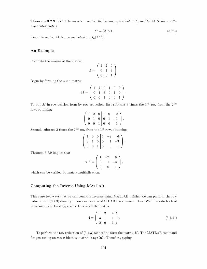
Theorem 3.7.9. Let A be an n " n matrix that is row equivalent to In and let M be the n " 2n

augmented matrixM = (A|In). (3.7.3)

Then the matrix M is row equivalent to (In|A#1).

An Example

Compute the inverse of the matrix

A =

!

"#1 2 00 1 30 0 1

$

%& .

Begin by forming the 3" 6 matrix

M =

!

"#1 2 0 1 0 00 1 3 0 1 00 0 1 0 0 1

$

%& .

To put M in row echelon form by row reduction, first subtract 3 times the 3rd row from the 2nd

row, obtaining !

"#1 2 0 1 0 00 1 0 0 1 !30 0 1 0 0 1

$

%& .

Second, subtract 2 times the 2nd row from the 1st row, obtaining!

"#1 0 0 1 !2 60 1 0 0 1 !30 0 1 0 0 1

$

%& .

Theorem 3.7.9 implies that

A#1 =

!

"#1 !2 60 1 !30 0 1

$

%& ,

which can be verified by matrix multiplication.

Computing the Inverse Using MATLAB

There are two ways that we can compute inverses using MATLAB . Either we can perform the rowreduction of (3.7.3) directly or we can use the MATLAB the command inv. We illustrate both ofthese methods. First type e3 7 4 to recall the matrix

A =

!

"#1 2 43 1 12 0 !1

$

%& . (3.7.4*)

To perform the row reduction of (3.7.3) we need to form the matrix M . The MATLAB commandfor generating an n" n identity matrix is eye(n). Therefore, typing

101

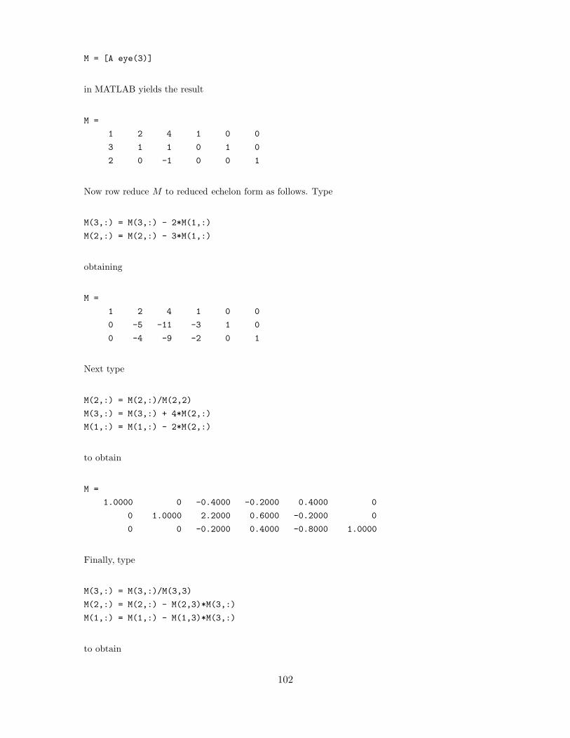
M = [A eye(3)]

in MATLAB yields the result

M =

1 2 4 1 0 0

3 1 1 0 1 0

2 0 -1 0 0 1

Now row reduce M to reduced echelon form as follows. Type

M(3,:) = M(3,:) - 2*M(1,:)

M(2,:) = M(2,:) - 3*M(1,:)

obtaining

M =

1 2 4 1 0 0

0 -5 -11 -3 1 0

0 -4 -9 -2 0 1

Next type

M(2,:) = M(2,:)/M(2,2)

M(3,:) = M(3,:) + 4*M(2,:)

M(1,:) = M(1,:) - 2*M(2,:)

to obtain

M =

1.0000 0 -0.4000 -0.2000 0.4000 0

0 1.0000 2.2000 0.6000 -0.2000 0

0 0 -0.2000 0.4000 -0.8000 1.0000

Finally, type

M(3,:) = M(3,:)/M(3,3)

M(2,:) = M(2,:) - M(2,3)*M(3,:)

M(1,:) = M(1,:) - M(1,3)*M(3,:)

to obtain

102

M =

1.0000 0 0 -1.0000 2.0000 -2.0000

0 1.0000 0 5.0000 -9.0000 11.0000

0 0 1.0000 -2.0000 4.0000 -5.0000

Thus C = A#1 is obtained by extracting the last three columns of M by typing

C = M(:,[4 5 6])

which yields

C =

-1.0000 2.0000 -2.0000

5.0000 -9.0000 11.0000

-2.0000 4.0000 -5.0000

You may check that C is the inverse of A by typing A*C and C*A.

In fact, this entire scheme for computing the inverse of a matrix has been preprogrammed intoMATLAB . Just type

inv(A)

to obtain

ans =

-1.0000 2.0000 -2.0000

5.0000 -9.0000 11.0000

-2.0000 4.0000 -5.0000

We illustrate again this simple method for computing the inverse of a matrix A. For example,reload the matrix in (3.1.4*) by typing e3_1_4 and obtaining:

A =

5 -4 3 -6 2

2 -4 -2 -1 1

1 2 1 -5 3

-2 -1 -2 1 -1

1 -6 1 1 4

The command B = inv(A) stores the inverse of the matrix A in the matrix B, and we obtain theresult

103

B =

-0.0712 0.2856 -0.0862 -0.4813 -0.0915

-0.1169 0.0585 0.0690 -0.2324 -0.0660

0.1462 -0.3231 -0.0862 0.0405 0.0825

-0.1289 0.0645 -0.1034 -0.2819 0.0555

-0.1619 0.0810 0.1724 -0.1679 0.1394

This computation also illustrates the fact that even when the matrix A has integer entries, theinverse of A usually has noninteger entries.

Let b = (2,!8, 18,!6,!1). Then we may use the inverse B = A#1 to compute the solution ofAx = b. Indeed if we type

b = [2;-8;18;-6;-1];

x = B*b

then we obtain

x =

-1.0000

2.0000

1.0000

-1.0000

3.0000

as desired (see (3.1.5*)). With this computation we have confirmed the analytical results of theprevious subsections.

Hand Exercises

1. Verify by matrix multiplication that the following matrices are inverses of each other:!

"#1 0 20 !1 21 0 1

$

%& and

!

"#!1 0 2

2 !1 !21 0 !1

$

%& .

2. Let $ #= 0 be a real number and let A be an invertible matrix. Show that the inverse of thematrix $A is given by 1

%A#1.

3. Let A =

'a 00 b

(be a 2" 2 diagonal matrix. For which values of a and b is A invertible?

4. Let A, B, C be general n" n matrices. Simplify the expression A#1(BA#1)#1(CB#1)#1.

In Exercises 5 – 6 use row reduction to find the inverse of the given matrix.

104

5.

!

"#1 4 50 1 !1!2 0 !8

$

%&.

6.

!

"#1 !1 !10 2 02 0 !1

$

%&.

7. Let A be an n " n matrix that satisfies

A3 + a2A2 + a1A + In = 0,

where A2 = AA and A3 = AA2. Show that A is invertible.Hint: Let B = !(A2 + a2A + a1In) and verify that AB = BA = In.

8. Let A be an n " n matrix that satisfies

Am + am#1Am#1 + · · ·+ a1A + In = 0.

Show that A is invertible.

9. For which values of a, b, c is the matrix

A =

!

"#1 a b

0 1 c

0 0 1

$

%&

invertible? Find A#1 when it exists.

Computer Exercises

In Exercises 10 – 11 use row reduction to find the inverse of the given matrix and confirm yourresults using the command inv.

10.

A =

!

"#2 1 31 2 35 1 0

$

%& . (3.7.5*)

11.

B =

!

"""#

0 5 1 31 5 3 !12 1 0 !41 7 2 3

$

%%%&. (3.7.6*)

12. Try to compute the inverse of the matrix

C =

!

"#1 0 3!1 2 !2

0 2 1

$

%& . (3.7.7*)

105

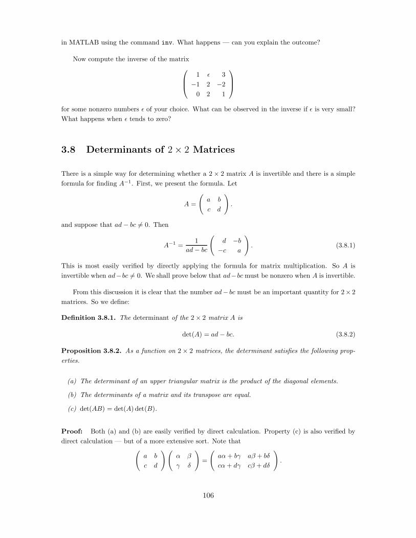
in MATLAB using the command inv. What happens — can you explain the outcome?

Now compute the inverse of the matrix!

"#1 + 3!1 2 !2

0 2 1

$

%&

for some nonzero numbers + of your choice. What can be observed in the inverse if + is very small?What happens when + tends to zero?

3.8 Determinants of 2 ! 2 Matrices

There is a simple way for determining whether a 2" 2 matrix A is invertible and there is a simpleformula for finding A#1. First, we present the formula. Let

A =

'a b

c d

(.

and suppose that ad! bc #= 0. Then

A#1 =1

ad! bc

'd !b

!c a

(. (3.8.1)

This is most easily verified by directly applying the formula for matrix multiplication. So A isinvertible when ad!bc #= 0. We shall prove below that ad!bc must be nonzero when A is invertible.

From this discussion it is clear that the number ad! bc must be an important quantity for 2" 2matrices. So we define:

Definition 3.8.1. The determinant of the 2" 2 matrix A is

det(A) = ad! bc. (3.8.2)

Proposition 3.8.2. As a function on 2" 2 matrices, the determinant satisfies the following prop-erties.

(a) The determinant of an upper triangular matrix is the product of the diagonal elements.

(b) The determinants of a matrix and its transpose are equal.

(c) det(AB) = det(A) det(B).

Proof: Both (a) and (b) are easily verified by direct calculation. Property (c) is also verified bydirect calculation — but of a more extensive sort. Note that

'a b

c d

( '$ %

& '

(=

'a$+ b& a% + b'

c$+ d& c% + d'

(.

106

Therefore,

det(AB) = (a$+ b&)(c% + d')! (a% + b')(c$+ d&)

= (ac$% + bc%& + ad$' + bd&') ! (ac$% + bc$' + ad%& + bd&')

= bc(%& ! $') + ad($' ! %&)

= (ad! bc)($' ! %&)

= det(A) det(B),

as asserted.

Corollary 3.8.3. A 2" 2 matrix A is invertible if and only if det(A) #= 0.

Proof: If A is invertible, then AA#1 = I2. Proposition 3.8.2 implies that

det(A) det(A#1) = det(I2) = 1.

Therefore, det(A) #= 0. Conversely, if det(A) #= 0, then (3.8.1) implies that A is invertible.

Determinants and Area

Suppose that v and w are two vectors in R2 that point in di"erent directions. Then, the set of points

z = $v + %w where 0 ( $, % ( 1

is a parallelogram, that we denote by P . We denote the area of P by |P |. For example, the unitsquare S, whose corners are (0, 0), (1, 0), (0, 1), and (1, 1), is the parallelogram generated by theunit vectors e1 and e2.

Next let A be a 2" 2 matrix and let

A(P ) = {Az : z % P}.

It follows from linearity (since Az = $Av + %Aw) that A(P ) is the parallelogram generated by Av

and Aw.

Proposition 3.8.4. Let A be a 2" 2 matrix and let S be the unit square. Then

|A(S)| = | det A|. (3.8.3)

Proof: Note that A(S) is the parallelogram generated by u1 = Ae1 and u2 = Ae2, and u1 and u2

are the columns of A. It follows that

(det A)2 = det(At) det(A) = det(AtA) = det

'ut

1u1 ut1u2

ut2u1 ut

2u2

(.

Hence

(det A)2 = det

'||u1||2 u1 · u2

u1 · u2 ||u2||2

(= ||u1||2||u2||2! (u1 · u2)2.

107

Recall that (1.4.5) of Chapter 1 states that

|P |2 = ||v||2||w||2! (v ·w)2.

where P is the parallelogram generated by v and w. Therefore, (det A)2 = |A(S)|2 and (3.8.3) isverified.

Theorem 3.8.5. Let P be a parallelogram in R2 and let A be a 2" 2 matrix. Then

|A(P )| = | det A||P |. (3.8.4)

Proof: First note that (3.8.3) a special case of (3.8.4), since |S| = 1. Next, let P be the parallel-ogram generated by the (column) vectors v and w, and let B = (v|w). Then P = B(S). It followsfrom (3.8.3) that |P | = | det B|. Moreover,

|A(P )| = |(AB)(S)|

= | det(AB)|

= | det A|| det B|

= | det A||P |,

as desired.

Hand Exercises

1. Find the inverse of the matrix '2 13 2

(.

2. Find the inverse of the shear matrix

'1 K

0 1

(.

3. Show that the 2 " 2 matrix A =

'a b

c d

(is row equivalent to I2 if and only if ad ! bc #= 0.

Hint: Prove this result separately in the two cases a #= 0 and a = 0.

4. Let A be a 2"2 matrix having integer entries. Find a condition on the entries of A that guaranteesthat A#1 has integer entries.

5. Let A be a 2" 2 matrix and assume that det(A) #= 0. Then use the explicit form for A#1 givenin (3.8.1) to verify that

det(A#1) =1

det(A).

6. Sketch the triangle whose vertices are 0, p = (3, 0)t, and q = (0, 2)t; and find the area of thistriangle. Let

M =

'!4 !3

5 !2

(.

Sketch the triangle whose vertices are 0, Mp, and Mq; and find the area of this triangle.

108

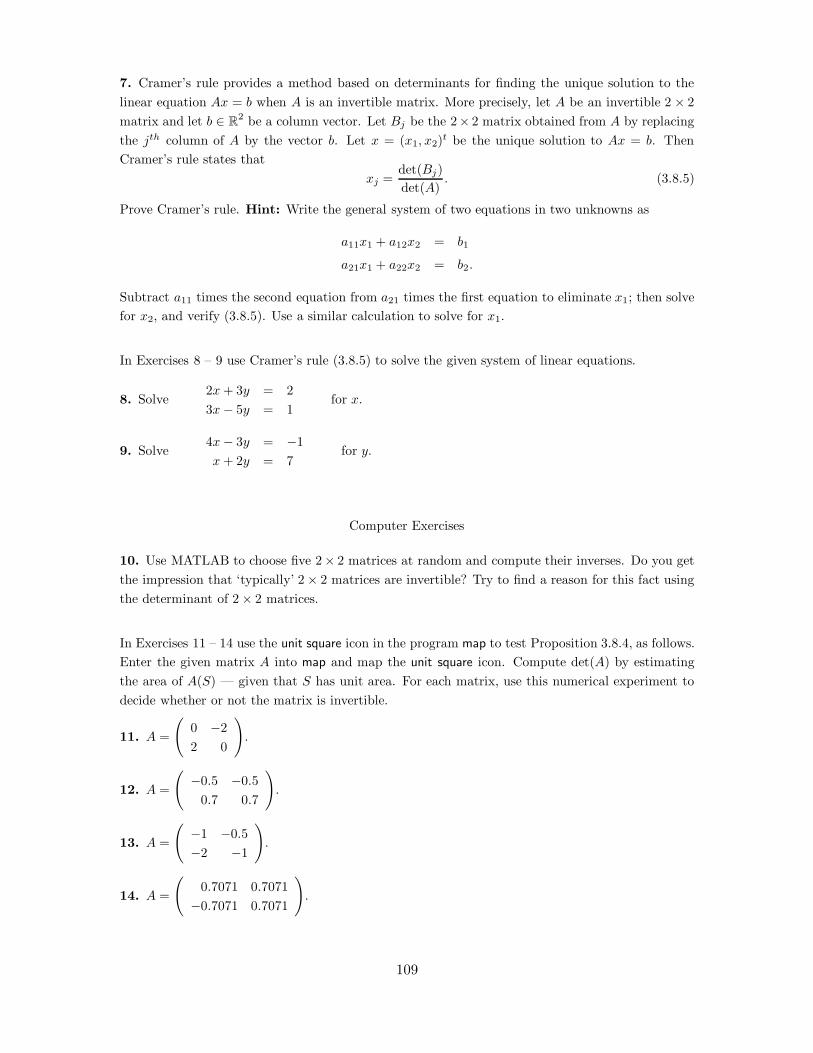
7. Cramer’s rule provides a method based on determinants for finding the unique solution to thelinear equation Ax = b when A is an invertible matrix. More precisely, let A be an invertible 2 " 2matrix and let b % R2 be a column vector. Let Bj be the 2" 2 matrix obtained from A by replacingthe jth column of A by the vector b. Let x = (x1, x2)t be the unique solution to Ax = b. ThenCramer’s rule states that

xj =det(Bj)det(A)

. (3.8.5)

Prove Cramer’s rule. Hint: Write the general system of two equations in two unknowns as

a11x1 + a12x2 = b1

a21x1 + a22x2 = b2.

Subtract a11 times the second equation from a21 times the first equation to eliminate x1; then solvefor x2, and verify (3.8.5). Use a similar calculation to solve for x1.

In Exercises 8 – 9 use Cramer’s rule (3.8.5) to solve the given system of linear equations.

8. Solve2x + 3y = 23x! 5y = 1

for x.

9. Solve4x! 3y = !1x + 2y = 7

for y.

Computer Exercises

10. Use MATLAB to choose five 2" 2 matrices at random and compute their inverses. Do you getthe impression that ‘typically’ 2" 2 matrices are invertible? Try to find a reason for this fact usingthe determinant of 2" 2 matrices.

In Exercises 11 – 14 use the unit square icon in the program map to test Proposition 3.8.4, as follows.Enter the given matrix A into map and map the unit square icon. Compute det(A) by estimatingthe area of A(S) — given that S has unit area. For each matrix, use this numerical experiment todecide whether or not the matrix is invertible.

11. A =

'0 !22 0

(.

12. A =

'!0.5 !0.5

0.7 0.7

(.

13. A =

'!1 !0.5!2 !1

(.

14. A =

'0.7071 0.7071!0.7071 0.7071

(.

109

Chapter 4

Determinants and Eigenvalues

In Section 3.8 we introduced determinants for 2 ! 2 matrices A. There we showed thatthe determinant of A is nonzero if and only if A is invertible. In Section 4.1 we generalizethe concept of determinants to n! n matrices. An alternative, more intuitive treatment ofdeterminants is given in Section 4.2.

If A is an n ! n matrix, then, as we noted in Section 3.2, A can be viewed as atransformation that maps an n-component vector to an n component vector; that is, A

can be thought of as a function from Rn into Rn. A number & is an eigenvalue of A

if there exists a nonzero vector v in Rn such that Av = &v. In Section 4.3 we usedeterminants to show that every n ! n matrix has exactly n eigenvalues. A treatment ofeigenvalues and eigenvectors is given in Section 4.4.

Certain details concerning determinants are deferred to Appendix 4.6.

4.1 Determinants

There are several equivalent ways to introduce determinants — none of which are easilymotivated. We prefer to define determinants through the properties they satisfy rather thanby formula. These properties actually enable us to compute determinants of n!n matriceswhere n > 3, which further justifies the approach. Later on, we will give an inductiveformula (4.1.9) for computing the determinant.

Definition 4.1.1. A determinant of a square n!n matrix A is a real number that satisfiesthe following three properties:

(a) If A = (aij) is lower triangular, then the determinant of A is the product of the

110

diagonal entries; that is,det(A) = a11 · · · · · ann.

(b) det(At) = det(A).

(c) Let B be an n ! n matrix. Then

det(AB) = det(A) det(B). (4.1.1)

Theorem 4.1.2. There exists a unique determinant function satisfying the three propertiesof Definition 4.1.1.

We will show that it is possible to compute the determinant of any n ! n matrix usingDefinition 4.1.1. Here we present a few examples:

Lemma 4.1.3. Let A be an n ! n matrix.

(a) Let c $ R be a scalar. Then det(cA) = cn det(A).

(b) If all of the entries in either a row or a column of A are zero, then det(A) = 0.

Proof: (a) Note that Definition 4.1.1(a) implies that det(cIn) = cn. It follows from (4.1.1)that

det(cA) = det(cInA) = det(cIn) det(A) = cn det(A).

(b) Definition 4.1.1(b) implies that it su!ces to prove this assertion when one row ofA is zero. Suppose that the ith row of A is zero. Let J be an n ! n diagonal matrix witha 1 in every diagonal entry except the ith diagonal entry which is 0. A matrix calculationshows that JA = A. It follows from Definition 4.1.1(a) that det(J) = 0 and from (4.1.1)that det(A) = 0.

Determinants of 2 " 2 Matrices

Before discussing how to compute determinants, we discuss the special case of 2!2 matrices.Recall from (3.8.2) of Section 3.8 that when

A =

'a b

c d

(

we defineddet(A) = ad " bc. (4.1.2)

111

We check that (4.1.2) satisfies the three properties in Definition 4.1.1. Observe that whenA is lower triangular, then b = 0 and det(A) = ad. So (a) is satisfied. It is straightforwardto verify (b). We already verified (c) in Chapter 3, Proposition 3.8.2.

It is less obvious perhaps — but true nonetheless — that the three properties of det(A)actually force the determinant of 2 ! 2 matrices to be given by formula (4.1.2). We beginby showing that Definition 4.1.1 implies that

det

'0 11 0

(

= "1. (4.1.3)

We verify this by observing that'

0 11 0

(=

'1 "10 1

('1 01 1

('1 00 "1

( '1 10 1

(. (4.1.4)

Hence property (c), (a) and (b) imply that

det

'0 11 0

(= 1 · 1 · ("1) · 1 = "1.

It is helpful to interpret the matrices in (4.1.4) as elementary row operations. Then (4.1.4)states that swapping two rows in a 2 ! 2 matrix is the same as performing the followingrow operations in order:

• add the 2nd row to the 1st row;

• multiply the 2nd row by "1;

• add the 1st row to the 2nd row; and

• subtract the 2nd row from the 1st row.

Suppose that d %= 0. Then

A =

'a b

c d

(

=

'1 b

d

0 1

( 'ad#bc

d 0c d

(

.

It follows from properties (c), (b) and (a) that

det(A) =ad " bc

dd = ad " bc,

as claimed.

Now suppose that d = 0 and note that

A =

'a b

c 0

(

=

'0 11 0

( 'c 0a b

(

.

112

Using (4.1.3) we see that

det(A) = " det

'c 0a b

(= "bc,

as desired.

We have verified that the only possible determinant function for 2 ! 2 matrices is thedeterminant function defined by (4.1.2).

Row Operations are Invertible Matrices

Proposition 4.1.4. Let A and B be m ! n matrices where B is obtained from A by asingle elementary row operation. Then there exists an invertible m!m matrix R such thatB = RA.

Proof: First consider multiplying the jth row of A by the nonzero constant c. Let R bethe diagonal matrix whose jth entry on the diagonal is c and whose other diagonal entriesare 1. Then the matrix RA is just the matrix obtained from A by multiplying the jth rowof A by c. Note that R is invertible when c %= 0 and that R#1 is the diagonal matrix whosejth entry is 1

c and whose other diagonal entries are 1. For example!

"#1 0 00 1 00 0 2

$

%&

!

"#a11 a12 a13

a21 a22 a23

a31 a32 a33

$

%& =

!

"#a11 a12 a13

a21 a22 a23

2a31 2a32 2a33

$

%& ,

multiplies the 3rd row by 2.

Next we show that the elementary row operation that swaps two rows may also bethought of as matrix multiplication. Let R = (rkl) be the matrix that deviates from theidentity matrix by changing in the four entries:

rii = 0

rjj = 0

rij = 1

rji = 1

A calculation shows that RA is the matrix obtained from A by swapping the ith and jth

rows. For example,!

"#0 0 10 1 01 0 0

$

%&

!

"#a11 a12 a13

a21 a22 a23

a31 a32 a33

$

%& =

!

"#a31 a32 a33

a21 a22 a23

a11 a12 a13

$

%& ,

113

which swaps the 1st and 3rd rows. Another calculation shows that R2 = In and hence thatR is invertible since R#1 = R.

Finally, we claim that adding c times the ith row of A to the jth row of A can be viewedas matrix multiplication. Let Ek! be the matrix all of whose entries are 0 except for theentry in the kth row and 'th column which is 1. Then R = In + cEij has the property thatRA is the matrix obtained by adding c times the jth row of A to the ith row. We can verifyby multiplication that R is invertible and that R#1 = In " cEij . More precisely,

(In + cEij)(In " cEij) = In + cEij " cEij " c2E2ij = In,

since E2ij = O for i %= j. For example,

(I3 + 5E12)A =

!

"#1 5 00 1 00 0 1

$

%&

!

"#a11 a12 a13

a21 a22 a23

a31 a32 a33

$

%&

=

!

"#a11 + 5a21 a12 + 5a22 a13 + 5a23

a21 a22 a23

a31 a32 a33

$

%& ,

adds 5 times the 2nd row to the 1st row.

Determinants of Elementary Row Matrices

Lemma 4.1.5. (a) The determinant of a swap matrix is "1.

(b) The determinant of the matrix that adds a multiple of one row to another is 1.

(c) The determinant of the matrix that multiplies one row by c is c.

Proof: The matrix that swaps the ith row with the jth row is the matrix whose nonzeroelements are akk = 1 where k %= i, j and aij = 1 = aji. Using a similar argument as in(4.1.3) we see that the determinants of these matrices are equal to "1.

The matrix that adds a multiple of one row to another is triangular (either upper orlower) and has 1’s on the diagonal. Thus property (a) in Definition 4.1.1 implies that thedeterminants of these matrices are equal to 1.

Finally, the matrix that multiplies the ith row by c %= 0 is a diagonal matrix all of whosediagonal entries are 1 except for aii = c. Again property (a) implies that the determinantof this matrix is c %= 0.

114

Computation of Determinants

We now show how to compute the determinant of any n!n matrix A using elementary rowoperations and Definition 4.1.1. It follows from Proposition 4.1.4 that every elementary rowoperation on A may be performed by premultiplying A by an elementary row matrix.

For each matrix A there is a unique reduced echelon form matrix E and a sequence ofelementary row matrices R1 . . .Rs such that

E = Rs · · ·R1A. (4.1.5)

It follows from Definition 4.1.1(c) that we can compute the determinant of A once we knowthe determinants of reduced echelon form matrices and the determinants of elementary rowmatrices. In particular

det(A) = det(E)/(det(R1) · · ·det(Rs)). (4.1.6)

It is easy to compute the determinant of any matrix in reduced echelon form usingDefinition 4.1.1(a) since all reduced echelon form n ! n matrices are upper triangular.Lemma 4.1.5 tells us how to compute the determinants of elementary row matrices. Thisdiscussion proves:

Proposition 4.1.6. If a determinant function exists for n ! n matrices, then it is unique.

We still need to show that determinant functions exist when n > 2. More precisely,we know that the reduced echelon form matrix E is uniquely defined from A (Chapter 2,Theorem 2.4.9), but there is more than one way to perform elementary row operations onA to get to E. Thus, we can write A in the form (4.1.6) in many di"erent ways, and thesedi"erent decompositions might lead to di"erent values for detA. (They don’t.)

An Example of Determinants by Row Reduction

As a practical matter we row reduce a square matrix A by premultiplying A by an elementaryrow matrix Rj . Thus

det(A) =1

det(Rj)det(RjA). (4.1.7)

We use this approach to compute the determinant of the 4 ! 4 matrix

A =

!

""""#

0 2 10 "21 2 4 01 6 1 "22 1 1 0

$

%%%%&.

115

The idea is to use (4.1.7) to keep track of the determinant while row reducing A to uppertriangular form. For instance, swapping rows changes the sign of the determinant; so

det(A) = " det

!

""""#

1 2 4 00 2 10 "21 6 1 "22 1 1 0

$

%%%%&.

Adding multiples of one row to another leaves the determinant unchanged; so

det(A) = " det

!

""""#

1 2 4 00 2 10 "20 4 "3 "20 "3 "7 0

$

%%%%&.

Multiplying a row by a scalar c corresponds to an elementary row matrix whose determinantis c. To make sure that we do not change the value of det(A), we have to divide thedeterminant by c as we multiply a row of A by c. So as we divide the second row of thematrix by 2, we multiply the whole result by 2, obtaining

det(A) = "2 det

!

""""#

1 2 4 00 1 5 "10 4 "3 "20 "3 "7 0

$

%%%%&.

We continue row reduction by zeroing out the last two entries in the 2nd column, obtaining

det(A) = "2 det

!

""""#

1 2 4 00 1 5 "10 0 "23 20 0 8 "3

$

%%%%&= 46 det

!

""""#

1 2 4 00 1 5 "10 0 1 " 2

23

0 0 8 "3

$

%%%%&.

Thus

det(A) = 46 det

!

""""#

1 2 4 00 1 5 "10 0 1 " 2

23

0 0 0 "5323

$

%%%%&= "106.

Determinants and Inverses

We end this subsection with an important observation about the determinant function.This observation generalizes to dimension n Corollary 3.8.3 of Chapter 3.

116

Theorem 4.1.7. An n ! n matrix A is invertible if and only if det(A) %= 0. Moreover, ifA#1 exists, then

det A#1 =1

detA. (4.1.8)

Proof: If A is invertible, then

det(A) det(A#1) = det(AA#1) = det(In) = 1.

Thus det(A) %= 0 and (4.1.8) is valid. In particular, the determinants of elementary row ma-trices are nonzero, since they are all invertible. (This point was proved by direct calculationin Lemma 4.1.5.)

If A is singular, then A is row equivalent to a non-identity reduced echelon form matrixE whose determinant is zero (since E is upper triangular and its last diagonal entry is zero).So it follows from (4.1.5) that

0 = det(E) = det(R1) · · ·det(Rs) det(A)

Since det(Rj) %= 0, it follows that det(A) = 0.

Corollary 4.1.8. If the rows of an n ! n matrix A are linearly dependent (for example, ifone row of A is a scalar multiple of another row of A), then det(A) = 0.

An Inductive Formula for Determinants

In this subsection we present an inductive formula for the determinant — that is, we assumethat the determinant is known for square (n " 1) ! (n " 1) matrices and use this formulato define the determinant for n! n matrices. This inductive formula is called expansion bycofactors .

Let A = (aij) be an n! n matrix. Let Aij be the (n" 1)! (n" 1) matrix formed fromA by deleting the ith row and the jth column. The matrices ("1)i+jAij are called cofactormatrices of A.

Inductively we define the determinant of an n ! n matrix A by:

det(A) =n)

j=1

("1)1+ja1j det(A1j)

= a11 det(A11) " a12 det(A12) + · · ·+ ("1)n+1a1n det(A1n). (4.1.9)

In Appendix 4.6 we show that the determinant function defined by (4.1.9) satisfies allproperties of a determinant function. Formula (4.1.9) is also called expansion by cofactorsalong the 1st row , since the a1j are taken from the 1st row of A. Since det(A) = det(At), it

117

follows that if (4.1.9) is valid as an inductive definition of determinant, then expansion bycofactors along the 1st column is also valid. That is,

det(A) = a11 det(A11) " a21 det(A21) + · · ·+ ("1)n+1an1 det(An1). (4.1.10)

We now explore some of the consequences of this definition, beginning with determinantsof small matrices. For example, Definition 4.1.1(a) implies that the determinant of a 1 ! 1matrix is just

det(a) = a.

Therefore, using (4.1.9), the determinant of a 2! 2 matrix is:

det

'a11 a12

a21 a22

(

= a11 det(a22) " a12 det(a21) = a11a22 " a12a21,

which is just the formula for determinants of 2 ! 2 matrices given in (4.1.2).

Similarly, we can now find a formula for the determinant of 3! 3 matrices A as follows.

det(A) = a11 det

'a22 a23

a32 a33

(" a12 det

'a21 a23

a31 a33

(+ a13 det

'a21 a22

a31 a32

(

(4.1.11)

= a11a22a33 + a12a23a31 + a13a21a32 " a11a23a32 " a12a21a33 " a13a22a31.

As an example, compute

det

!

"#2 1 41 "1 35 6 "2

$

%&

using formula (4.1.11) as

2("1)("2)+ 1 · 3 · 5 + 4 · 6 · 1" 4("1)5" 3 · 6 · 2" ("2)1 · 1 = 4+ 15+ 24+ 20" 36+ 2 = 29.

There is a visual mnemonic for remembering how to compute the six terms in formula(4.1.11) for the determinant of 3 ! 3 matrices. Write the matrix as a 3 ! 5 array byrepeating the first two columns, as shown in bold face in Figure 4.1: Then add the productof terms connected by solid lines sloping down and to the right and subtract the products ofterms connected by dashed lines sloping up and to the right. Warning: this nice crisscrossalgorithm for computing determinants of 3!3 matrices does not generalize to n!n matrices.

When computing determinants of n!n matrices when n > 3, it is usually more e!cientto compute the determinant using row reduction rather than by using formula (4.1.9). Inthe appendix to this chapter, Section 4.6, we verify that formula (4.1.9) actually satisfiesthe three properties of a determinant, thus completing the proof of Theorem 4.1.2.

118

a11 a12 a13

a21 a22 a23

a31 a32 a33 a31

a21

a11

a32

a22

a12

Figure 4.1: Mnemonic for computation of determinants of 3 ! 3 matrices.

An interesting and useful formula for reducing the e"ort in computing determinants isgiven by the following formula.

Lemma 4.1.9. Let A be an n ! n matrix of the form

A =

'B 0C D

(

,

where B is a k ! k matrix and D is an (n " k) ! (n " k) matrix. Then

det(A) = det(B) det(D).

Proof: We prove this result using (4.1.9) coupled with induction. Assume that this lemmais valid or all (n"1)!(n"1) matrices of the appropriate form. Now use (4.1.9) to compute

det(A) = a11 det(A11) " a12 det(A12) + · · · ± a1n det(A1n)

= b11 det(A11) " b12 det(A12) + · · · ± b1k det(A1k).

Note that the cofactor matrices A1j are obtained from A by deleting the 1st row and thejth column. These matrices all have the form

A1j =

'B1j 0Cj D

(,

where Cj is obtained from C by deleting the jth column. By induction on k

det(A1j) = det(B1j) det(D).

It follows that

det(A) = (b11 det(B11) " b12 det(B12) + · · · ± b1k det(B1k)) det(D)

= det(B) det(D),

as desired.

119

Determinants in MATLAB

The determinant function has been preprogrammed in MATLAB and is quite easy to use.For example, typing e8 1 11 will load the matrix

A =

!

""""#

1 2 3 02 1 4 1

"2 "1 0 1"1 0 "2 3

$

%%%%&.

To compute the determinant of A just type det(A) and obtain the answer

ans =

-46

Alternatively, we can use row reduction techniques in MATLAB to compute the deter-minant of A — just to test the theory that we have developed. Note that to compute thedeterminant we do not need to row reduce to reduced echelon form — we need only reduceto an upper triangular matrix. This can always be done by successively adding multiplesof one row to another — an operation that does not change the determinant. For example,to clear the entries in the 1st column below the 1st row, type

A(2,:) = A(2,:) - 2*A(1,:);

A(3,:) = A(3,:) + 2*A(1,:);

A(4,:) = A(4,:) + A(1,:)

obtaining

A =

1 2 3 0

0 -3 -2 1

0 3 6 1

0 2 1 3

To clear the 2nd column below the 2nd row type

A(3,:) = A(3,:) + A(2,:);A(4,:) = A(4,:) - A(4,2)*A(2,:)/A(2,2)

obtaining

120

A =

1.0000 2.0000 3.0000 0

0 -3.0000 -2.0000 1.0000

0 0 4.0000 2.0000

0 0 -0.3333 3.6667

Finally, to clear the entry (4, 3) type

A(4,:) = A(4,:) -A(4,3)*A(3,:)/A(3,3)

to obtain

A =

1.0000 2.0000 3.0000 0

0 -3.0000 -2.0000 1.0000

0 0 4.0000 2.0000

0 0 0 3.8333

To evaluate the determinant of A, which is now an upper triangular matrix, type

A(1,1)*A(2,2)*A(3,3)*A(4,4)

obtaining

ans =

-46

as expected.

Hand Exercises

In Exercises 1 – 3 compute the determinants of the given matrix.

1. A =

!

"#!2 1 0

4 5 01 0 2

$

%&.

2. B =

!

"""#

1 0 2 3!1 !2 3 2

4 !2 0 31 2 0 !3

$

%%%&.

121

3. C =

!

""""""#

2 1 !1 0 01 !2 3 0 0!3 2 !2 0 0

1 1 !1 2 40 2 3 !1 !3

$

%%%%%%&.

4. Find det(A#1) where A =

!

"#!2 !3 2

4 1 3!1 1 1

$

%&.

5. Two n " n matrices A and B are similar if there exists an n " n matrix P such thatB = P#1AP . Show that the determinants of similar n " n matrices are equal.

In Exercises 6 – 8 use row reduction to compute the determinant of the given matrix.

6. A =

!

"#!1 !2 1

3 1 3!1 1 1

$

%&.

7. B =

!

"""#

1 0 1 00 1 0 !11 0 !1 00 1 0 1

$

%%%&.

8. C =

!

"""#

1 2 0 10 2 1 0!2 !3 3 !1

1 0 5 2

$

%%%&.

9. Let

A =

!

"#2 !1 00 3 01 5 3

$

%& and B =

!

"#2 0 00 !1 00 0 3

$

%& .

(a) For what values of ( is det((A !B) = 0?

(b) Is there a vector x for which Ax = Bx?

In Exercises 10 – 11 verify that the given matrix has determinant !1.

10. A =

!

"#1 0 00 0 10 1 0

$

%&.

11. B =

!

"#0 0 10 1 01 0 0

$

%&.

12. Compute the cofactor matrices A13, A22, A21 when A =

!

"#3 2 !40 1 50 0 6

$

%&.

122

13. Compute the cofactor matrices B11, B23, B43 when B =

!

"""#

0 2 !4 5!1 7 !2 10

0 0 0 !13 4 2 !10

$

%%%&.

14. Find values of ( where the determinant of the matrix

A& =

!

"#( ! 1 0 !1

0 (! 1 1!1 1 (

$

%&

vanishes.

15. Suppose that two n" p matrices A and B are row equivalent. Show that there is an invertiblen" n matrix P such that B = PA.

16. Let A be an invertible n " n matrix and let b % Rn be a column vector. Let Bj be the n " n

matrix obtained from A by replacing the jth column of A by the vector b. Let x = (x1, . . . , xn)t bethe unique solution to Ax = b. Then Cramer’s rule states that

xj =det(Bj)det(A)

. (4.1.12)

Prove Cramer’s rule. Hint: Let Aj be the jth column of A so that Aj = Aej . Show that

Bj = A(e1| · · · |ej#1|x|ej+1| · · · |en).

Using this product, compute the determinant of Bj and verify (4.1.12).

123

4.2 Determinants, An Alternative Treatment

Associated with each n"n matrix A is a number called its determinant. We will give an inductivedevelopment of this concept, beginning with the determinant of a 2" 2 matrix. Then we’ll expressa 3 " 3 determinant as a sum of 2 " 2 determinants, a 4 " 4 determinant as a sum of 3 " 3determinants, and so on.

Consider the system of two linear equations in two unknowns

ax + by = $

cx + dy = %

We eliminate the y unknown by multiplying the first equation by d, the second equation by!b, and adding. This gives

(ad! bc)x = d$! b%.

This equation has the solution x =d$! b%

ad! bc, provided ad! bc #= 0.

Similarly, we can solve the system for the y unknown by multiplying the first equation by !c,the second equation by a, and adding. This gives

(ad! bc)y = a% ! c$

which has the solution y =a% ! c$

ad ! bc, again provided ad! bc #= 0.

The matrix of coe!cients of the system is A =

'a b

c d

(. The number ad! bc is called the

determinant of A. The determinant of A is denoted by det A and by00000

a b

c d

00000 .

The determinant has a geometric interpretation in this 2" 2 case.

The graph of the first equation ax+by = $ is a straight line with slope !a/b, provided b #= 0.The graph of the second equation is a straight line with slope !c/d, provided d #= 0. (If b = 0 ord = 0, then the corresponding line is vertical.) Assume that b, d #= 0. If

!a

b#= !c

d,

then the lines have di"erent slopes and the system of equations has a unique solution. However,

!a

b#= !c

dis equivalent to ad! bc #= 0.

Thus, det A #= 0 implies that the system has a unique solution.

On the other hand, if ad ! bc = 0, then!a

b=!c

d(assuming b, d #= 0), and the two lines

have the same slope. In this case, the lines are either parallel (the system has no solutions), or thelines coincide (the system has infinitely many solutions).

124

In general, an n" n matrix A is said to be nonsingular if det A #= 0; A is singular ifdet A = 0.

Look again at the solutions

x =d$! b%

ad! bc, y =

a% ! c$

ad ! bc, ad! bc #= 0.

The two numerators also have the form of a determinant of a 2 " 2 matrix. In particular, thesesolutions can be written as

x =

00000$ b

% d

0000000000

a b

c d

00000

, y =

00000a $

c %

0000000000

a b

c d

00000

This representation of the solutions of a system of two equations in two unknowns is the n = 2version of a general result known as Cramer’s rule.

Example 1. Given the system of equations

5x! 2y = 8

3x + 4y = 10

Verify that the determinant of the matrix of coe!cients is nonzero and solve the system usingCramer’s rule.

SOLUTION The matrix of coe!cients is A =

'5 !23 4

(and det A = 26. According to Cramer’s

rule,

x =

000008 !2

10 4

0000000000

5 !22 4

00000

=5226

= 2, y =

000005 83 10

0000000000

5 !22 4

00000

=2626

= 1

The solution set is x = 2, y = 1. !

Now we’ll go to 3" 3 matrices.

The determinant of a 3 ! 3 matrix

If

A =

!

"#a1 a2 a3

b1 b2 b3

c1 c2 c3

$

%&,

then

det A =

0000000

a1 a2 a3

b1 b2 b3

c1 c2 c3

0000000= a1b2c3 ! a1b3c2 + a2b3c1 ! a2b1c3 + a3b1c2 ! a3b2c1.

125

The problem with this definition is that it is hard to remember. Fortunately the expression onthe right can be written conveniently in terms of 2" 2 determinants as follows:

det A = a1b2c3 ! a1b3c2 + a2b3c1 ! a2b1c3 + a3b1c2 ! a3b2c1

= a1(b2c3 ! b3c2)! a2(b1c3 ! b3c1) + a3(b1c2 ! b2c1)

= a1

00000b2 b3

c2 c3

00000! a2

00000b1 b3

c1 c3

00000 + a3

00000b1 b2

c1 c2

00000

This representation of a 3 " 3 determinant is called the expansion of the determinant across thefirst row. Notice that the coe!cients are the entries a1, a2, a3 of the first row, that they occuralternately with + and ! signs, and that each is multiplied by a 2 " 2 determinant. You canremember the determinant that goes with each entry ai as follows: in the original matrix, mentallycross out the row and column containing ai and take the determinant of the 2 " 2 matrix thatremains.

Example 2. Let A =

!

"#3 !2 !42 5 !10 6 1

$

%& and B =

!

"#7 6 51 2 13 !2 1

$

%&. Calculate det A and det B.

SOLUTION

det A = 3

000005 !16 1

00000! (!2)

000002 !10 1

00000 + (!4)

000002 50 6

00000

= 3[(5)(1)! (!1)(6)] + 2[(2)(1)! (!1)(0)]! 4[(2)(6)! (5)(0)]

= 3(11) + 2(2)! 4(12) = !11

det B = 7

000002 1!2 1

00000! 6

000001 13 1

00000 + 5

000001 23 !2

00000

= 7[(2)(1)! (1)(!2)]! 6[(1)(1)! (1)(3)] + 5[(1)(!2)! (2)(3)]

= 7(4)! 6(!2) + 5(!8) = 0. !

There are other ways to group the terms in the definition. For example

det A = a1b2c3 ! a1b3c2 + a2b3c1 ! a2b1c3 + a3b1c2 ! a3b2c1

= !a2(b1c3 ! b3c1) + b2(a1c3 ! a3c1)! c2(a1c3 ! a3c1)

= !a2

00000b1 b3

c1 c3

00000 + b2

00000a1 a3

c1 c3

00000 + !c2

00000a1 a3

b1 b3

00000

This is called the expansion of the determinant down the second column.

In general, depending on how you group the terms in the definition, you can expand across anyrow or down any column. The signs of the coe!cients in the expansion across a row or down acolumn are alternately +, !, starting with a + in the (1,1)-position. The pattern of signs is:

!

"#+ ! +! + !+ ! +

$

%&

126

Example 3. Let A =

!

"#3 !2 !42 5 !10 6 1

$

%& and C =

!

"#7 0 51 0 13 !2 1

$

%&.

1. Calculate det A by expanding down the first column.

det A = 3

000005 !16 1

00000! 2

00000!2 !4

6 1

00000 + 0

00000!2 !4

5 !1

00000

= 3[(5)(1)! (!1)(6)]! 2[(!2)(1)! (!4)(6)] + 0

= 3(11)! 2(22) + 0 = !11

2. Calculate det A by expanding across the third row.

det A = 0

00000!2 !4

5 !1

00000! 6

000003 !42 !1

00000 + (1)

000003 !22 5

00000

= 0! 6[(3)(!1)! (!4)(2)] + [(3)(5)! (!2)(2)]

= !6(5) + (19) = !11

3. Calculate det C by expanding down the second column.

det C = !0

000001 13 1

00000 + 0

000007 53 1

00000! (!2)

000007 51 1

00000

= 0 + 0 + 2(2) = 14

Notice the advantage of expanding across a row or down a column that contains one or morezeros. !

Now consider the system of three equations in three unknowns

a11x + a12y + a13z = b1

a21x + a22y + a23z = b2

a31x + a32y + a33z = b2

Writing this system in vector-matrix form, we have!

""#

a11 a12 a13

a21 a22 a23

a31 a32 a33

$

%%&

!

"#x1

x2

x3

$

%& =

!

"#b1

b2

b3

$

%&

It can be shown that if det A #= 0, then the system has a unique solution which is given by

x1 =det A1

det A, x2 =

det A2

det A, x3 =

det A3

det A

where

A1 =

!

""#

b1 a12 a13

b2 a22 a23

b3 a32 a33

$

%%& , A2 =

!

""#

a11 b1 a13

a21 b2 a23

a31 b3 a33

$

%%& , and A3 =

!

""#

a11 a12 b1

a21 a22 b2

a31 a32 b3

$

%%&

127

This is Cramer’s rule in the 3" 3 case.

If det A = 0, then the system either has infinitely many solutions or no solutions.

Example 4. Given the system of equations

2x + y ! z = 3

x + y + z = 1

x! 2y ! 3z = 4

.

Verify that the determinant of the matrix of coe!cients is nonzero and find the value of y usingCramer’s rule.

SOLUTION The matrix of coe!cients is A =

!

"#2 1 !11 1 11 !2 !3

$

%& and det A = 5.

According to Cramer’s rule

y =

0000000

2 3 !11 1 11 4 !3

0000000

5=!55

= !1. !

The determinant of a 4 ! 4 matrix

Following the pattern suggested by the calculation of a 3 " 3 determinant, we’ll express a 4 " 4determinant as the sum of four 3" 3 determinants. For example, the expansion of

det A =

000000000

a1 a2 a3 a4

b1 b2 b3 b4

c1 c2 c3 c4

d1 d2 d3 d4

000000000

across the first row is

det A = a1

0000000

b2 b3 b4

c2 c3 c4

d2 d3 d4

0000000! a2

0000000

b1 b3 b4

c1 c3 c4

d1 d3 d4

0000000+ a3

0000000

b1 b2 b4

c1 c2 c4

d1 d2 d4

0000000+ a4

0000000

b1 b2 b3

c1 c2 c3

d1 d2 d3

0000000

As in the 3 " 3 case, you can calculate a 4" 4 determinant by expanding across any row ordown any column. The matrix of signs associated with a 4" 4 determinant is

!

"""#

+ ! + !! + ! ++ ! + !! + ! +

$

%%%&

128

Cramer’s Rule

Here is the general version of Cramer’s rule: Given the system of n equations in n unknowns

a11x1 + a12x2 + a13x3 + · · ·+ a1nxn = b1

a21x1 + a22x2 + a23x3 + · · ·+ a2nxn = b2

a31x1 + a32x2 + a33x3 + · · ·+ a3nxn = b3

.........................................................

an1x1 + an2x2 + an3x3 + · · ·+ annxn = bn

(1)

If det A #= 0, then the system has a unique solution x1, x2, . . . , xn given by

x1 =det A1

det A, x2 =

det A2

det A, . . . , xn =

det An

det A

where det Ai is the determinant obtained by replacing the ith column of det A by the column!

""""#

b1

b2

...bn

$

%%%%&

i = 1, 2, . . . , n.

If det A = 0, then the system either has no solution or infinitely many solutions. In the specialcase of a homogeneous system, det A = 0 implies that the system has infinitely many nontrivialsolutions.

Properties of Determinants

It should now be clear how to calculate an n" n determinant for any n. However, for n > 3 thecalculations, while simple in theory, tend to be long, tedious, and involved. Although the determinantis a complicated mathematical function (its domain is the set of square matrices, its range is the setof real numbers), it does have certain properties that can be used to simplify calculations.

Before listing the properties of determinants, we give the determinants of some special types ofmatrices.

1. If an n" n matrix A has a row of zeros, or a column of zeros, then det A = 0; an n " n

matrix with a row of zeros or a column of zeros is singular. (Simply expand across the row orcolumn of zeros.)

2. An n"n matrix is said to be upper triangular if all of its entries below the main diagonal arezero. (Recall that the entries a11, a22, a33, . . . , ann form the main diagonal of an n " n

matrix A.) A 4" 4 upper triangular matrix has the form

T =

!

"""#

a11 a12 a13 a14

0 a22 a23 a24

0 0 a33 a34

0 0 0 a44

$

%%%&

129

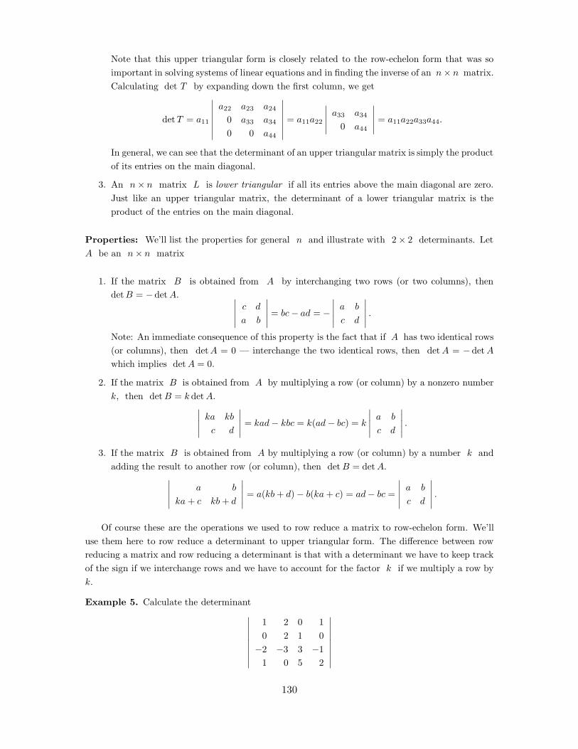
Note that this upper triangular form is closely related to the row-echelon form that was soimportant in solving systems of linear equations and in finding the inverse of an n" n matrix.Calculating det T by expanding down the first column, we get

det T = a11

0000000

a22 a23 a24

0 a33 a34

0 0 a44

0000000= a11a22

00000a33 a34

0 a44

00000 = a11a22a33a44.

In general, we can see that the determinant of an upper triangular matrix is simply the productof its entries on the main diagonal.

3. An n" n matrix L is lower triangular if all its entries above the main diagonal are zero.Just like an upper triangular matrix, the determinant of a lower triangular matrix is theproduct of the entries on the main diagonal.

Properties: We’ll list the properties for general n and illustrate with 2" 2 determinants. LetA be an n" n matrix

1. If the matrix B is obtained from A by interchanging two rows (or two columns), thendet B = ! det A. 00000

c d

a b

00000 = bc! ad = !

00000a b

c d

00000 .

Note: An immediate consequence of this property is the fact that if A has two identical rows(or columns), then det A = 0 — interchange the two identical rows, then det A = ! det A

which implies det A = 0.

2. If the matrix B is obtained from A by multiplying a row (or column) by a nonzero numberk, then det B = k det A.

00000ka kb

c d

00000 = kad! kbc = k(ad! bc) = k

00000a b

c d

00000 .

3. If the matrix B is obtained from A by multiplying a row (or column) by a number k andadding the result to another row (or column), then det B = det A.

00000a b

ka + c kb + d

00000 = a(kb + d)! b(ka + c) = ad! bc =

00000a b

c d

00000 .

Of course these are the operations we used to row reduce a matrix to row-echelon form. We’lluse them here to row reduce a determinant to upper triangular form. The di"erence between rowreducing a matrix and row reducing a determinant is that with a determinant we have to keep trackof the sign if we interchange rows and we have to account for the factor k if we multiply a row byk.

Example 5. Calculate the determinant000000000

1 2 0 10 2 1 0!2 !3 3 !1

1 0 5 2

000000000

130

SOLUTION

000000000

1 2 0 10 2 1 0!2 !3 3 !1

1 0 5 2

000000000

=2R1+R3, #R1+r4

000000000

1 2 0 10 2 1 00 1 3 10 !2 5 1

000000000

=R2%R3

!

000000000

1 2 0 10 1 3 10 2 1 00 !2 5 1

000000000

=#2R2+R3&R3, 2R2+R4&R4

!

000000000

1 2 0 10 1 3 10 0 !5 !20 0 11 3

000000000

=#(1/5)R3&R3

5

000000000

1 2 0 10 1 3 10 0 1 2/50 0 11 3

000000000

=#11R3+R4&R4

5

000000000

1 2 0 10 1 3 10 0 1 2/50 0 0 !7/5

000000000

= 5!75

= !7

Note, we could have stopped at

!

000000000

1 2 0 10 1 3 10 0 !5 !20 0 11 3

000000000

and calculated

!

000000000

1 2 0 10 1 3 10 0 !5 !20 0 11 3

000000000

= !(1)(1)

00000!5 !211 3

00000 = !(!15 + 22) = !7. !

Inverse, determinant and rank

We have seen that a system of equations Ax = b where A is an n" n matrix has a uniquesolution if and only if A has an inverse. We have also seen that the system has a unique solutionif and only if det A #= 0; that is, if and only if A is nonsingular. It now follows that A hasan inverse if and only if det A #= 0. Thus, the determinant provides a test as to whether an n " n

matrix has an inverse.

There is also the connection with rank: an n" n matrix has an inverse if and only if its rank isn.

Putting all this together we have the following equivalent statements:

1. The system of equations Ax = b, A an n " n matrix, has a unique solution.

131

2. A has an inverse.

3. det A #= 0.

4. A has rank n.

Exercises 4.2

Use the determinant to decide whether the matrix has an inverse. If it exists, find it and verifyyour answer by calculating AA#1.

1.

'2 03 1

(

2.

'0 1!2 4

(

3.

'1 23 4

(

4.

'1 2!2 !4

(

5.

!

"#1 0 22 !1 34 1 8

$

%&

6.

!

"#1 2 !4!1 !1 52 7 !3

$

%&

7.

!

"#1 3 !41 5 !13 13 !6

$

%&

8.

!

"#1 2 30 1 24 5 3

$

%&

9.

!

"""#

1 1 !1 20 2 0 !1!1 2 2 !20 !1 0 1

$

%%%&

10.

!

"""#

1 1 0 00 1 1 01 0 1 00 0 1 1

$

%%%&

132

11. Each of the matrices in Problems 1 - 10 has integer entries. In some cases the inverse matrixalso had integer entries, in other cases it didn’t. Suppose A is an n" n matrix with integerentries. Make a conjecture as to when A#1, if it exists, will also have integer entries.

Solve the system of equations by finding the inverse of the matrix of coe!cients.

12.x + 2y = 23x + 5y = 4

13.x + 3y = 52x + y = 10

14.2x + 4y = 23x + 8y = 1

15.2x + y = 44x + 3y = 3

16.x! 3y = 2y + z = !2

2x! y + 4z = 1

17.x + 2y ! z = 2x + y + 2z = 0x! y ! z = 1

18.!x + y = 5!x + z = !2

6x! 2y ! 3z = 1

Evaluate the determinant in two ways, using the indicated row and column expansions

19.

0000000

0 3 21 5 7!2 !6 !1

0000000; across the 2nd row, down the 1st column.

20.

0000000

1 2 !32 5 !83 8 !13

0000000; across the 3rd row, down the 2nd column.

21.

0000000

5 !1 23 0 6!4 3 1

0000000; across the 2nd row, down the 3rd column.

22.

0000000

2 !3 05 !2 02 0 !1

0000000; across the 3rd row, down the 3nd column.

23.

0000000

1 0 32 !2 14 0 !3

0000000; across the 1st row, down the 2nd column.

Evaluate the determinant using the row or column that minimizes the amount of computation.

133

24.

0000000

1 3 02 5 !23 4 0

0000000

25.

0000000

2 !5 10 3 03 4 !2

0000000

26.

0000000

1 3 02 5 !23 4 0

0000000

27.

0000000

1 3 !42 0 !20 0 3

0000000

28.

000000000

1 !2 3 04 0 5 07 !3 2 2!3 0 4 0

000000000

29.

000000000

2 !1 3 41 0 5 2!2 0 0 2!2 0 !1 4

000000000

30. Find the values of x such that

00000x + 1 x

3 x! 2

00000 = 3.

31. Find the values of x such that

0000000

x 0 22x x! 1 4!x x! 1 x + 1

0000000= 0.

Determine whether Cramer’s rule applies. If it does, solve for the indicated unknown

32.2x! y + 3z = 1

y + 2z = !3x + z = 0

; x =?

33.!4x + y = 3

2x + 2y + z = !23x + 4z = 2

; y =?

34.3x + z = !2

x + 2y ! z = 0x! 4y + 3z = 1

; z =?

35.!2x! y = 3

x + 3y ! z = 05y ! 2z = 3

; z =?

134

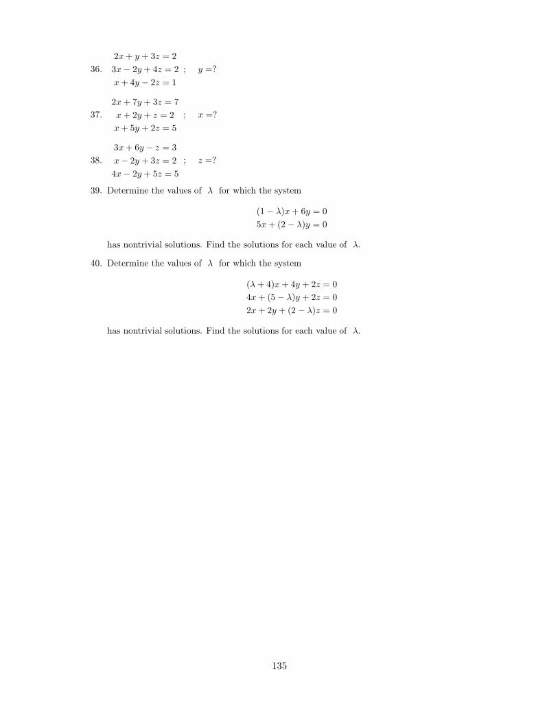
36.2x + y + 3z = 23x! 2y + 4z = 2x + 4y ! 2z = 1

; y =?

37.2x + 7y + 3z = 7x + 2y + z = 2x + 5y + 2z = 5

; x =?

38.3x + 6y ! z = 3x! 2y + 3z = 24x! 2y + 5z = 5

; z =?

39. Determine the values of ( for which the system

(1! ()x + 6y = 05x + (2 ! ()y = 0

has nontrivial solutions. Find the solutions for each value of (.

40. Determine the values of ( for which the system

(( + 4)x + 4y + 2z = 04x + (5! ()y + 2z = 02x + 2y + (2 ! ()z = 0

has nontrivial solutions. Find the solutions for each value of (.

135

4.3 Eigenvalues

In this section we discuss how to find eigenvalues for an n"n matrix A. A number ( is an eigenvalueof A if there exists a nonzero eigenvector v such that

Av = (v. (4.3.1)

The vector v is called an eigenvector corresponding to the eigenvalue (. It follows that the matrixA! (In is singular since

(A! (In)v = 0.

Theorem 4.1.7 implies thatdet(A ! (In) = 0.

With these observations in mind, we can make the following definition.

Definition 4.3.1. Let A be an n" n matrix. The characteristic polynomial of A is:

pA(() = det(A ! (In).

In Theorem 4.3.3 we show that pA(() is indeed a polynomial of degree n in (. Note here thatthe roots of pA are the eigenvalues of A. As we discussed, the real eigenvalues of A are rootsof the characteristic polynomial. Conversely, if ( is a real root of pA, then Theorem 4.1.7 statesthat the matrix A ! (In is singular and therefore that there exists a nonzero vector v such that(4.3.1) is satisfied. Similarly, by using this extended algebraic definition of eigenvalues we allowthe possibility of complex eigenvalues. The complex analog of Theorem 4.1.7 shows that if ( is acomplex eigenvalue, then there exists a nonzero complex n-vector v such that (4.3.1) is satisfied.

Example 4.3.2. Let A be an n " n lower triangular matrix. Then the diagonal entries are theeigenvalues of A. We verify this statement as follows.

A! (In =

!

""#

a11 ! ( 0.. .

(&) ann ! (

$

%%& .

Since the determinant of a triangular matrix is the product of the diagonal entries, it follows that

pA(() = (a11 ! () · · · (ann ! (), (4.3.2)

and hence that the diagonal entries of A are roots of the characteristic polynomial. A similarargument works if A is upper triangular.

It follows from (4.3.2) that the characteristic polynomial of a triangular matrix is a polynomialof degree n and that

pA(() = (!1)n(n + bn#1(n#1 + · · ·+ b0. (4.3.3)

for some real constants b0, . . . , bn#1. In fact, this statement is true in general.

Theorem 4.3.3. Let A be an n"n matrix. Then pA is a polynomial of degree n of the form (4.3.3).

136

Proof: Let C be an n " n matrix whose entries have the form cij + dij(. Then det(C) is apolynomial in ( of degree at most n. We verify this statement by induction. It is easily verifiedwhen n = 1, since then C = (c + d() for some real numbers c and d. Then det(C) = c + d( whichis a polynomial of degree at most one. (It may have degree zero, if d = 0.) So assume that thisstatement is true for (n! 1)" (n ! 1) matrices. Recall from (4.1.9) that

det(C) = (c11 + d11() det(C11) + · · ·+ (!1)n+1(c1n + d1n() det(C1n).

By induction each of the determinants C1j is a polynomial of degree at most n ! 1. It followsthat multiplication by c1j + d1j( yields a polynomial of degree at most n in (. Since the sum ofpolynomials of degree at most n is a polynomial of degree at most n, we have verified our assertion.

Since A!(In is a matrix whose entries have the desired form, it follows that pA(() is a polynomialof degree at most n in (. To complete the proof of this theorem we need to show that the coe!cientof (n is (!1)n. Again, we verify this statement by induction. This statement is easily verified for1 " 1 matrices — we assume that it is true for (n ! 1) " (n ! 1) matrices. Again use (4.1.9) tocompute

det(A! (In) = (a11 ! () det(B11) ! a12 det(B12) + · · ·+ (!1)n+1a1n det(B1n).

where B1j are the cofactor matrices of A ! (In. Using our previous observation all of the termsdet(B1j) are polynomials of degree at most n ! 1. Thus, in this expansion, the only term that cancontribute a term of degree n is:

!( det(B11).

Note that the cofactor matrix B11 is the (n! 1) " (n! 1) matrix

B11 = A11 ! (In#1,

where A11 is the first cofactor matrix of the matrix A. By induction, det(B11) is a polynomial ofdegree n!1 with leading term (!1)n#1(n#1. Multiplying this polynomial by !( yields a polynomialof degree n with the correct leading term.

General Properties of Eigenvalues

The fundamental theorem of algebra states that every polynomial of degree n has exactly n roots(counting multiplicity). For example, the quadratic formula shows that every quadratic polynomialhas exactly two roots. In general, the proof of the fundamental theorem is not easy and is certainlybeyond the limits of this course. Indeed, the di!culty in proving the fundamental theorem of algebrais in proving that a polynomial p(() of degree n > 0 has one (complex) root. Suppose that (0 is aroot of p((); that is, suppose that p((0) = 0. Then it is easy to show that

p(() = (( ! (0)q(() (4.3.4)

for some polynomial q of degree n ! 1. So once we know that p has a root, then we can argue byinduction to prove that p has n roots.

Recall that a polynomial need not have any real roots. For example, the polynomial p(() = (2+1has no real roots, since p(() > 0 for all real (. This polynomial does have two complex roots±i = ±

$!1.

137

However, a polynomial with real coe!cients has either real roots or complex roots that come incomplex conjugate pairs. To verify this statement, we need to show that if (0 is a complex root ofp((), then so is (0. We claim that

p(() = p(().

To verify this point, suppose that

p(() = cn(n + cn#1(

n#1 + · · ·+ c0,

where each cj % R. Then

p(() = cn(n + cn#1(n#1 + · · ·+ c0 = cn(n

+ cn#1(n#1

+ · · ·+ c0 = p(()

If (0 is a root of p((), thenp((0) = p((0) = 0 = 0.

Hence (0 is also a root of p.

It follows that

Theorem 4.3.4. Every (real) n"n matrix A has exactly n eigenvalues (1, . . . ,(n. These eigenvaluesare either real or complex conjugate pairs. Moreover,

(a) pA(() = ((1 ! () · · · ((n ! (),

(b) det(A) = (1 · · ·(n.

Proof: Since the characteristic polynomial pA is a polynomial of degree n with real coe!cients,the first part of the theorem follows from the preceding discussion. In particular, it follows from(4.3.4) that

pA(() = c((1 ! () · · · ((n ! (),

for some constant c. Formula (4.3.3) implies that c = 1 — which proves (a). Since pA(() =det(A! (In), it follows that pA(0) = det(A). Thus (a) implies that pA(0) = (1 · · ·(n, thus proving(b).

The eigenvalues of a matrix do not have to be di"erent. For example, consider the extreme caseof a strictly triangular matrix A. Example 4.3.2 shows that all of the eigenvalues of A are zero.

We now discuss certain properties of eigenvalues.

Corollary 4.3.5. Let A be an n " n matrix. Then A is invertible if and only if zero is not aneigenvalue of A.

Proof: The proof follows from Theorem 4.1.7 and Theorem 4.3.4(b).

Lemma 4.3.6. Let A be a singular n " n matrix. Then the null space of A is the span of alleigenvectors whose associated eigenvalue is zero.

Proof: An eigenvector v of A has eigenvalue zero if and only if

Av = 0.

This statement is valid if and only if v is in the null space of A.

138

Theorem 4.3.7. Let A be an invertible n" n matrix with eigenvalues (1, · · · ,(n. Then the eigen-values of A#1 are (#1

1 , · · · ,(#1n .

Proof: We claim thatpA(() = (!1)n det(A)(npA"1 (

1(

).

It then follows that 1& is an eigenvalue for A#1 for each eigenvalue ( of A. This makes sense, since

the eigenvalues of A are nonzero.

Compute:

(!1)n det(A)(npA"1 (1(

) = (!()n det(A) det(A#1 ! 1(

In)

= det(!(A) det(A#1 ! 1(

In)

= det(!(A(A#1 ! 1(

In))

= det(A ! (In)

= pA((),

which verifies the claim.

Theorem 4.3.8. Let A and B be similar n" n matrices. Then

pA = pB ,

and hence the eigenvalues of A and B are identical.

Proof: Since B and A are similar, there exists an invertible n"n matrix S such that B = S#1AS.It follows that

det(B ! (In) = det(S#1AS ! (In) = det(S#1(A ! (In)S) = det(A ! (In),

which verifies that pA = pB.

Recall that the trace of an n " n matrix A is the sum of the diagonal entries of A; that is

tr(A) = a11 + · · ·+ ann.

We state without proof the following theorem:

Theorem 4.3.9. Let A be an n" n matrix with eigenvalues (1, . . . ,(n. Then

tr(A) = (1 + · · ·+ (n.

It follows from Theorem 4.3.8 that the traces of similar matrices are equal.

MATLAB Calculations

The commands for computing characteristic polynomials and eigenvalues of square matrices arestraightforward in MATLAB . In particular, for an n"n matrix A, the MATLAB command poly(A)

returns the coe!cients of (!1)npA(().

139

For example, reload the 4"4 matrix A of (4.1) by typing e8 1 11. The characteristic polynomialof A is found by typing

poly(A)

to obtain

ans =

1.0000 -5.0000 15.0000 -10.0000 -46.0000

Thus the characteristic polynomial of A is:

pA(() = (4 ! 5(3 + 15(2 ! 10(! 46.

The eigenvalues of A are found by typing eig(A) and obtaining

ans =

-1.2224

1.6605 + 3.1958i

1.6605 - 3.1958i

2.9014

Thus A has two real eigenvalues and one complex conjugate pair of eigenvalues. Note that MAT-LAB has preprogrammed not only the algorithm for finding the characteristic polynomial, but alsonumerical routines for finding the roots of the characteristic polynomial.

The trace of A is found by typing trace(A) and obtaining

ans =

5

Using the MATLAB command sum we can verify the statement of Theorem 4.3.9. Indeed sum(v)

computes the sum of the components of the vector v and typing

sum(eig(A))

we obtain the answer 5.0000, as expected.

Hand Exercises

In Exercises 1 – 2 determine the characteristic polynomial and the eigenvalues of the given matrices.

140

1. A =

!

"#!9 !2 !10

3 2 38 2 9

$

%&.

2. B =

!

"""#

2 1 !5 21 2 13 20 0 3 !10 0 1 1

$

%%%&.

3. Find the eigenvectors of

A =

!

"#3 1 !1!1 1 1

2 2 0

$

%&

corresponding to the eigenvalue ( = 2.

4. Consider the matrix

A =

!

"#!1 1 1

1 !1 11 1 !1

$

%& .

(a) Verify that the characteristic polynomial of A is p&(A) = ((! 1)((+ 2)2.

(b) Show that (1, 1, 1) is an eigenvector of A corresponding to ( = 1.

(c) Show that (1, 1, 1) is orthogonal to every eigenvector of A corresponding to the eigenvalue( = !2.

5. Consider the matrix A =

'8 5

!10 !7

(.

(a) Find the eigenvalues and eigenvectors of A.

(b) Express the vector (a, b) as a linear combination of the vectors found in (a).

6. Find the characteristic polynomial and the eigenvalues of

A =

!

"#!1 2 2

2 2 2!3 !6 !6

$

%& .

Find eigenvectors corresponding to each of the three eigenvalues.

7. Let A be an n " n matrix. Suppose that

A2 + A + In = 0.

Prove that A is invertible.

In Exercises 8 – 9 decide whether the given statements are true or false. If the statements are false,give a counterexample; if the statements are true, give a proof.

141

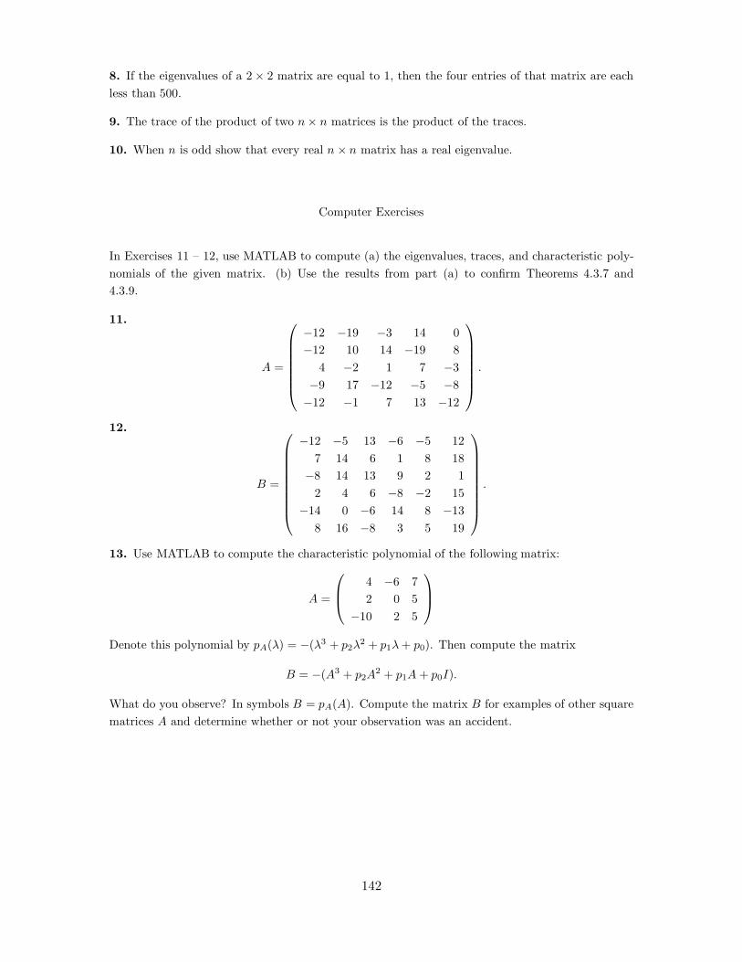
8. If the eigenvalues of a 2" 2 matrix are equal to 1, then the four entries of that matrix are eachless than 500.

9. The trace of the product of two n" n matrices is the product of the traces.

10. When n is odd show that every real n " n matrix has a real eigenvalue.

Computer Exercises

In Exercises 11 – 12, use MATLAB to compute (a) the eigenvalues, traces, and characteristic poly-nomials of the given matrix. (b) Use the results from part (a) to confirm Theorems 4.3.7 and4.3.9.

11.

A =

!

""""""#

!12 !19 !3 14 0!12 10 14 !19 8

4 !2 1 7 !3!9 17 !12 !5 !8!12 !1 7 13 !12

$

%%%%%%&.

12.

B =

!

""""""""#

!12 !5 13 !6 !5 127 14 6 1 8 18!8 14 13 9 2 1

2 4 6 !8 !2 15!14 0 !6 14 8 !13

8 16 !8 3 5 19

$

%%%%%%%%&

.

13. Use MATLAB to compute the characteristic polynomial of the following matrix:

A =

!

"#4 !6 72 0 5

!10 2 5

$

%&

Denote this polynomial by pA(() = !((3 + p2(2 + p1(+ p0). Then compute the matrix

B = !(A3 + p2A2 + p1A + p0I).

What do you observe? In symbols B = pA(A). Compute the matrix B for examples of other squarematrices A and determine whether or not your observation was an accident.

142

4.4 Eigenvalues and Eigenvectors

Here is an alternative discussion of eigenvalues and eigenvectors.

Let A be an n" n matrix. Then A can be viewed as a transformation that maps ann-component vector to an n component vector; that is, A can be thought of as a function fromRn into Rn. Here’s an example.

Example 1. Let A be the 3" 3 matrix!

"#2 2 31 2 12 !2 1

$

%&.

Then A maps the vector ( 2, !1, 3 ) to ( 11, 3, 9 ):!

"#2 2 31 2 12 !2 1

$

%&

!

"#2!1

3

$

%& =

!

"#1139

$

%& ;

A maps the vector (!1, 2, 3 ) to the vector ( 10, 7, !6 ):!

"#2 2 31 2 12 !2 1

$

%&

!

"#!1

23

$

%& =

!

"#107!6

$

%& ;

and, in general, !

"#2 2 31 2 12 !2 1

$

%&

!

"#a

b

c

$

%& =

!

"#2a + 2b + 3c

a + 2b + c

2a! 2b + c

$

%& .

Now consider the vector v = ( 8, 5, 2 ). It has a special property relative to A:!

"#2 2 31 2 12 !2 1

$

%&

!

"#852

$

%& =

!

"#32208

$

%& = 4

!

"#852

$

%& ;

A maps v = ( 8, 5, 2 ) to a multiple of itself; Av = 4v.

You can also verify that!

"#2 2 31 2 12 !2 1

$

%&

!

"#23!2

$

%& = 2

!

"#23!2

$

%& and

!

"#2 2 31 2 12 !2 1

$

%&

!

"#10!1

$

%& = (!1)

!

"#10!1

$

%& .

This is the property that we will study in this section.

Definition 4.4.1. Let A be an n" n matrix. A number ( is an eigenvalue of A if thereexists a nonzero vector v in Rn such that

Av = (v.

The vector v is called an eigenvector corresponding to (.

143

In Example 1, the numbers 4, 2, !1 are eigenvalues of A and v = ( 8, 5, 2 ), u =( 2, 3, !2 ), w = ( 1, 0, !1 ) are corresponding eigenvectors.

Eigenvalues (vectors) are also called characteristic values (vectors) or proper values (vectors).

Calculating the Eigenvalues of a Matrix

Let A be an n" n matrix and suppose that ( is an eigenvalue of A with correspondingeigenvector v. Then

Av = (v implies Av ! (v = 0.

The latter equation can be written(A ! (In)v = 0.

This equation says that the homogeneous system of linear equations

(A ! (In)x = 0

has the nontrivial solution v. As we saw in Section 5.6, a homogeneous system of n linear equationsin n unknowns has a nontrivial solution if and only if the determinant of the matrix of coe!cientsis zero. Thus, ( is an eigenvalue of A if and only if

det(A ! (In) = 0.

The equation det(A! (In) = 0 is called the characteristic equation of the matrix A. The roots ofthe characteristic equation are the eigenvalues of A.

We’ll start with a special case which we’ll illustrate with a 3" 3 matrix.

Example 2. Let A be an upper triangular matrix:

A =

!

"#a1 a2 a3

0 b2 b3

0 0 c3

$

%&.

Then the eigenvalues of A are the entries on the main diagonal.

det(A ! (I3) =

0000000

a1 ! ( a2 a3

0 b2 ! ( b3

0 0 c3 ! (

0000000= (a1 ! ()(b2 ! ()(c3 ! ().

Thus, the eigenvalues of A are: (1 = a1, (2 = b2, (3 = c3.

The general result is this: If A is either an upper triangular matrix or a lower triangular matrix,then the eigenvalues of A are the entries on the main diagonal of A.

Now we’ll look at arbitrary matrices; that is, no special form.

Example 3. Find the eigenvalues of

A =

'1 !3!2 2

(.

144

SOLUTION We need to find the numbers ( that satisfy the equation det(A ! (I2) = 0:

A! (I2 =

'1 !3!2 2

(! (

'1 00 1

(=

'1! ( !3!2 2! (

(

and 000001! ( !3!2 2! (

00000 = (1! ()(2! () ! 6 = (2 ! 3(! 4 = (( + 1)(( ! 4).

Therefore the eigenvalues of A are (1 = !1 and (2 = 4.

Example 4. Find the eigenvalues of

A =

!

"#1 !3 1!1 1 1

3 !3 !1

$

%&.

SOLUTION We need to find the numbers ( that satisfy the equation det(A ! (I3) = 0:

A! (I3 =

!

"#1 !3 1!1 1 1

3 !3 !1

$

%&! (

!

"#1 0 00 1 00 0 1

$

%& =

!

"#1! ( !3 1!1 1! ( 1

3 !3 !1 ! (

$

%&

and

det A =

0000000

1! ( !3 1!1 1! ( 1

3 !3 !1! (

0000000.

Expanding across the first row (remember, you can go across any row or down any column), we have0000000

1! ( !3 1!1 1! ( 1

3 !3 !1! (

0000000= (1! () [(1! ()(!1 ! () + 3] + 3 [1 + (! 3] + [3! 3(1! ()]

= !(3 + (2 + 4(! 4 = !(( + 2)(( ! 1)(( ! 2).

Therefore the eigenvalues of A are (1 = !2, (2 = 1, (3 = 2.

Note that the characteristic equation of our 2" 2 matrix is a polynomial equation of degree 2,a quadratic equation; the characteristic equation of our 3" 3 matrix is a polynomial equation ofdegree 3; a cubic equation. This is true in general. That is, the characteristic equation of an n " n

matrix A is 0000000000

a11 ! ( a12 · · · a1n

a21 a22 ! ( · · · a2n

...... · · ·

...an1 a2n · · · ann ! (

0000000000

= p(() = 0,

where p is a polynomial of degree n in (. The polynomial p is called the characteristic polynomialof A.

Recall the following facts about a polynomial p of degree n with real coe!cients.

145

1. p has exactly n roots, counting multiplicities.

2. p may have complex roots, but if a + bi is a root, then its conjugate a! bi is also a root;the complex roots of p occur in conjugate pairs, counting multiplicities.

3. p can be factored into a product of linear and quadratic factors — the linear factors cor-responding to the real roots of p and the quadratic factors corresponding to the complexroots.

Example 5. Calculate the eigenvalues of

A =

'1 !14 1

(.

SOLUTION 000001! ( !1

4 1! (

00000 = (1! ()2 + 4 = (2 ! 2(+ 5.

The roots of (2 ! 2(+ 5 = 0 are (1 = 1 + 2i, (2 = 1! 2i; A has complex eigenvalues.

Example 6. Calculate the eigenvalues of

A =

!

"#1 !3 33 !5 36 !6 4

$

%&.

SOLUTION 0000000

1! ( !3 33 !5! ( 36 !6 4! (

0000000= !(3 + 12(+ 16 = !(( + 2)2((! 4).

The eigenvalues of A are (1 = (2 = !2, (3 = 4; !2 is an eigenvalue of multiplicity 2.

Calculating the Eigenvectors of a Matrix

We note first that if ( is an eigenvalue of an n" n matrix A and v is a correspondingeigenvector, then any nonzero multiple of v is also an eigenvector of A corresponding to (: ifAv = (v and r is any nonzero number, then

A(rv) = rAv = r((v) = ((r v).

Thus, each eigenvalue has infinitely many corresponding eigenvectors.

Let A be an n" n matrix. If ( is an eigenvalue of A with corresponding eigenvector v,then v is a solution of the homogeneous system of equations

(A! ( In)x = 0. (1)

Therefore, to find an eigenvector of A corresponding to the eigenvalue (, we need to find anontrivial solution of (1). This takes us back to the solution methods of Sections 2.3 and 2.4.

146

Example 7. Find the eigenvalues and corresponding eigenvectors of'

2 41 !1

(.

SOLUTION The first step is to find the eigenvalues.

det(A! (I2) =

000002! ( 4

1 !1! (

00000 = (2 ! ( ! 6 = ((! 3)((+ 2).

The eigenvalues of A are (1 = 3, (2 = !2.

Next we find an eigenvector for each eigenvalue. Equation (1) for this problem is'

2! ( 41 !1! (

(x =

'2! ( 4

1 !1! (

('x1

x2

(= (0, 0) . (2)

We have to deal with each eigenvalue separately. We set ( = 3 in (2) to get'!1 4

1 !4

( 'x1

x2

(= 0.

The augmented matrix for this system of equations is'!1 4 0

1 !4 0

(

which row reduces to '1 !4 00 0 0

(.

The solution set is x1 = 4a, x2 = a, a any real number.

We get an eigenvector by choosing a value for a. Since an eigenvector is, by definition, a nonzerovector, we must choose an a #= 0. Any such a will do; we’ll let a = 1. Then, an eigenvectorcorresponding to the eigenvalue (1 = 3 is v1 = (4, 1). Here is a verification:

'2 41 !1

( '41

(=

'123

(= 3

'41

(.

Now we set ( = !2 in (2) to get'

4 41 1

( 'x1

x2

(= 0.

The augmented matrix for this system of equations is'

4 4 01 1 0

(

which row reduces to '1 1 00 0 0

(.

147

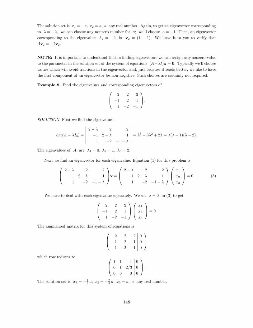
The solution set is x1 = !a, x2 = a, a any real number. Again, to get an eigenvector correspondingto ( = !2, we can choose any nonzero number for a; we’ll choose a = !1. Then, an eigenvectorcorresponding to the eigenvalue (2 = !2 is v2 = (1, !1). We leave it to you to verify thatAv2 = !2v2.

NOTE: It is important to understand that in finding eigenvectors we can assign any nonzero valueto the parameter in the solution set of the system of equations (A!(I)x = 0. Typically we’ll choosevalues which will avoid fractions in the eigenvector and, just because it reads better, we like to havethe first component of an eigenvector be non-negative. Such choices are certainly not required.

Example 8. Find the eigenvalues and corresponding eigenvectors of!

"#2 2 2!1 2 1

1 !2 !1

$

%&.

SOLUTION First we find the eigenvalues.

det(A ! (I3) =

0000000

2! ( 2 2!1 2! ( 1

1 !2 !1! (

0000000= (3 ! 3(2 + 2( = ((( ! 1)(( ! 2).

The eigenvalues of A are (1 = 0, (2 = 1, (3 = 2.

Next we find an eigenvector for each eigenvalue. Equation (1) for this problem is!

"#2! ( 2 2!1 2! ( 1

1 !2 !1! (

$

%&x =

!

"#2! ( 2 2!1 2! ( 1

1 !2 !1 ! (

$

%&

!

"#x1

x2

x3

$

%& = 0. (3)

We have to deal with each eigenvalue separately. We set ( = 0 in (3) to get!

"#2 2 2!1 2 1

1 !2 !1

$

%&

!

"#x1

x2

x3

$

%& = 0.

The augmented matrix for this system of equations is!

"#2 2 2 0!1 2 1 0

1 !2 !1 0

$

%&

which row reduces to !

"#1 1 1 00 1 2/3 00 0 0 0

$

%& .

The solution set is x1 = !13 a, x2 = !2

3 a, x3 = a, a any real number.

148

We get an eigenvector by choosing a value for a. We’ll choose a = !3 (this avoids havingfractions as components, a convenience). Thus, an eigenvector corresponding to the eigenvalue(1 = 0 is v1 = ( 1, 2, !3 ). Here is a verification:

!

"#2 2 2!1 2 1

1 !2 !1

$

%&

!

"#12!3

$

%& =

!

"#000

$

%& = 0

!

"#12!3

$

%& .

Next we set ( = 1 in (3) to get!

"#1 2 2!1 1 1

1 !2 !2

$

%&

!

"#x1

x2

x3

$

%& = 0.

The augmented matrix for this system of equations is!

"#1 2 2 0!1 1 1 0

1 !2 !2 0

$

%&

which row reduces to !

"#1 2 2 00 1 1 00 0 0 0

$

%& .

The solution set is x1 = 0, x2 = !a, x3 = a, a any real number. If we let a = !1, we get theeigenvector v2 = ( 0, 1, !1 ). You can verify that Av2 = v2.

Finally, we set ( = 2 in (3) to get!

"#1 2 2!1 1 1

1 !2 !2

$

%&

!

"#x1

x2

x3

$

%& = 0.

The augmented matrix for this system of equations is!

"#0 2 2 0!1 0 1 0

1 !2 !3 0

$

%&

which row reduces to !

"#1 0 !1 00 1 1 00 0 0 0

$

%& .

The solution set is x1 = a, x2 = !a, x3 = a, a any real number. If we let a = 1, we get theeigenvector v3 = ( 1, !1, 1 ). You can verify that Av3 = v3.

We have been working mainly with real numbers but the need to consider complex numbersarises here — the characteristic polynomial of an n" n matrix A may have complex roots. Ofcourse, since the characteristic polynomial has real coe!cients, complex roots occur in conjugatepairs. Also, we have to expect that an eigenvector corresponding to a complex eigenvalue will becomplex; that is, have complex number components. Here is the main theorem in this regard.

149

Theorem 4.4.2. Let A be a (real) n" n matrix. If the complex number ( = a + bi is aneigenvalue of A with corresponding (complex) eigenvector u+ iv, then ( = a! bi, the conjugateof a + bi, is also an eigenvalue of A and u! iv is a corresponding eigenvector.

The proof is a simple application of complex arithmetic:

A(u + iv) = (a + bi)(u + iv)

A(u + iv) = (a + bi)(u + iv) (the overline denotes complex conjugate)

A (u + iv) = (a + bi) (u + iv)

A(u! iv) = (a! bi)(u! iv)

Example 9. As we saw in Example 4, the matrix

A =

'1 !14 1

(.

has the complex eigenvalues (1 = 1 + 2i, (2 = 1 ! 2i. We’ll find the eigenvectors. The nice thingabout a pair of complex eigenvalues is that we only have to calculate one eigenvector. Equation (1)for this problem is

'1! ( !1

4 1! (

(x =

'1! ( !1

4 1! (

( 'x1

x2

(= 0.

Substituting (1 = 1 + 2i in this equation gives'!2i !1

4 !2i

(x =

'!2i !1

4 !2i

('x1

x2

(=

'00

(.

The augmented matrix for this system of equations is'!2i !1 0

4 !2i 0

(

which row reduces to '1 !1

2 i 00 0 0

(.

The solution set is x1 = 12 i a, x2 = a, a any number; in this case, either real or complex. If we

set x2 = !2i, we get the eigenvector v1 = (1, !2i) = (1, 0) + i (0, !2):'

1 !14 1

( '1

!2i

(=

'1 + 2i

4! 2i

(= (1 + 2i)

'1

!2i

(.

Now, by Theorem 2, an eigenvector corresponding to (2 = 1! 2i is v2 = (1, 0)! i (0, !2).

Eigenvalues of multiplicity greater than 1 can cause di!culties which we will investigate laterin the text. These di!culties carry over into other fields, such as di"erential equations. In the nexttwo examples we’ll illustrate what can happen when an eigenvalue has multiplicity 2.

150

Example 10. Find the eigenvalues and eigenvectors of

A =

!

"#1 !3 33 !5 36 !6 4

$

%&.

SOLUTION First we find the eigenvalues:

det(A! (I3) =

0000000

1! ( !3 33 !5( 36 !6 4! (

0000000= 16 + 12(! (3 = !(( ! 4)((+ 2)2.

The eigenvalues of A are (1 = 4, (2 = (3 = !2; !2 is an eigenvalue of multiplicity 2.

You can verify that v1 = ( 1, 1, 2 ) is an eigenvector corresponding to (1 = 4.

Now we investigate what happens with the eigenvalue !2:

(A! (!2)I3)x =

!

"#3 !3 33 !3 36 !6 6

$

%&

!

"#x1

x2

x3

$

%& =

!

"#000

$

%& . (a)

The augmented matrix for this system of equation is!

"#3 !3 3 03 !3 3 06 !6 6 0

$

%&

which row reduces to !

"#1 !1 1 00 0 0 00 0 0 0

$

%& .

The solution set of the corresponding system of equations is x1 = a ! b, a, b any real numbers.We can assign any values we want to a and b, except a = b = 0 (an eigenvector is a nonzerovector). Setting a = 1, b = 0 gives the eigenvector v2 = ( 1, 1, 0 ); setting a = 0, b = !1 givesthe eigenvector v3 = ( 1, 0, !1 ).

Note that our two choices of a and b produced two linearly independent eigenvectors (thevectors are not multiples of each other). The fact that the solution set of the system of equations(a) had two independent parameters guarantees that we can obtain two independent eigenvectors.

Example 11. Find the eigenvalues and eigenvectors of

A =

!

"#5 6 20 !1 !81 0 !2

$

%&.

SOLUTION First we find the eigenvalues:

det(A! (I3) =

0000000

5! ( 6 20 !1 ! ( !81 0 !2! (

0000000= !36 + 15(+ 2(2 ! (3 = !(( + 4)((! 3)2.

151

The eigenvalues of A are (1 = !4, (2 = (3 = 3; 3 is an eigenvalue of multiplicity 2.

You can verify that v1 = ( 6, !8, !3 ) is an eigenvector corresponding to (1 = !4.

We now find the eigenvectors for 3:

(A! 3I3)x =

!

"#2 6 20 !4 !81 0 !5

$

%&

!

"#x1

x2

x3

$

%& =

!

"#000

$

%& . (b)

The augmented matrix for this system of equation is!

"#2 6 2 00 !4 !8 01 0 !5 0

$

%&

which row reduces to !

"#1 3 1 00 1 2 00 0 0 0

$

%& .

The solution set of the corresponding system of equations is x1 = 5a, x2 = !2a, x3 = a, a anyreal number. Setting a = 1 gives the eigenvector v2 = ( 5, !2, 1 )

In this case, the eigenvalue of multiplicity two yielded only one (independent) eigenvector.

In general, if the matrix A has an eigenvalue ( of multiplicity k, then ( may have only one(independent) eigenvector, it may have two independent eigenvectors, it may have three independenteigenvectors, and so on, up to k independent eigenvectors. It can be shown using Theorem 2 that( cannot have more than k linearly independent eigenvectors.

Eigenvalues, Determinant, Inverse, Rank

There is a relationship between the eigenvalues of an n" n matrix A, the determinant of A, theexistence of A#1, and the rank of A.

Theorem 4.4.3. Let A be an n" n matrix with eigenvalues (1, (2, . . . , (n. (Note: the (’shere are not necessarily distinct, one or more of the eigenvalues may have multiplicity greater than1, and they are not necessarily real.) Then

det A = (1 · (2 · (3 · · · · (n.

That is, det A is the product of the eigenvalues of A.

Proof: The eigenvalues of A are the roots of the characteristic polynomial

det(A! (I) = p(().

Writing p(() in factored form, we have

det(A! (I) = p(() = ((1 ! ()((2 ! ()((3 ! () · · · ((n ! ().

Setting ( = 0, we getdet A = (1 · (2 · (3 · · · ·(n.

152

At the end of Section 5.6 we listed equivalences between the determinant, existence of an inverseand rank. With Theorem 3, we can add eigenvalues to the list of equivalences.

Let A be an n" n matrix. The following are equivalent:

1. The system of equations Ax = b has a unique solution.

2. A has an inverse.

3. det A #= 0.

4. A has rank n.

5. 0 is not an eigenvalue of A

Exercises 4.4

Determine the eigenvalues and the eigenvectors.

1. A =

'2 !10 3

(.

2. A =

'3 12 0

(.

3. A =

'1 23 2

(.

4. A =

'1 42 3

(.

5. A =

'6 5!5 !4

(.

6. A =

'!1 1

4 2

(.

7. A =

'3 !11 1

(.

8. A =

'1 !11 1

(.

9. A =

'2 !11 2

(.

10. A =

!

"#3 2 !2!3 !1 3

1 2 0

$

%&. Hint: 1 is an eigenvalue.

153

11. A =

!

"#15 7 !7!1 1 113 7 !5

$

%&. Hint: 2 is an eigenvalue.

12. A =

!

"#2 !2 11 !1 1!3 2 !2

$

%&. Hint: 1 is an eigenvalue.

13. A =

!

"#2 1 11 2 1!2 !2 !1

$

%&. Hint: 1 is an eigenvalue.

14. A =

!

"#1 !3 10 1 03 0 !1

$

%&. Hint: 1 is an eigenvalue.

15. A =

!

"#0 1 1!1 1 1!1 1 1

$

%&.

16. A =

!

"#1 !4 !13 2 31 1 3

$

%&. Hint: 2 is an eigenvalue.

17. A =

!

"#!1 1 2!1 1 1!2 1 3

$

%&.

18. A =

!

"#2 2 11 3 11 2 2

$

%&. Hint: 5 is an eigenvalue.

19. A =

!

"#1 !2 2!2 1 2!2 0 3

$

%&. Hint: 3 is an eigenvalue.

20. A =

!

"#4 1 !12 5 !21 1 2

$

%&. Hint: 3 is an eigenvalue.

21. A =

!

"""#

4 2 !2 21 3 1 !10 0 2 01 1 !3 5

$

%%%&. Hint: 2 is an eigenvalue of multiplicity 2.

22. A =

!

"""#

3 5 !5 53 1 3 !3!2 2 0 2

0 4 !6 8

$

%%%&. Hint: 2 and !2 are eigenvalues.

23. Prove that if ( is an eigenvalue of A, then for every positive integer k, (k is an eigenvalueof Ak.

154

24. Suppose that ( is a nonzero eigenvalue of A with corresponding eigenvector v. Prove thatif A has an inverse, then 1/( is an eigenvalue of A#1 with corresponding vector v.

155

4.5 *Markov Chains

MARKOV CHAINS

Markov chains provide an interesting and useful application of matrices and linear algebra. Inthis section we introduce Markov chains via some of the theory and two examples. The theory canbe understood and applied to examples using just the background in linear algebra that we havedeveloped in this chapter.

An Example of Cats

Consider the four room apartment pictured in Figure 4.2. One way passages between the rooms areindicated by arrows. For example, it is possible to go from room 1 directly to any other room, butwhen in room 3 it is possible to go only to room 4.

1 2

3 4Figure 4.2: Schematic design of apartment passages.

Suppose that there is a cat in the apartment and that at each hour the cat is asked to move fromthe room that it is in to another. True to form, however, the cat chooses with equal probability tostay in the room for another hour or to move through one of the allowed passages. Suppose thatwe let pij be the probability that the cat will move from room i to room j; in particular, pii is theprobability that the cat will stay in room i. For example, when the cat is in room 1, it has fourchoices — it can stay in room 1 or move to any of the other rooms. Assuming that each of thesechoices is made with equal probability, we see that

p11 =14

p12 =14

p13 =14

p14 =14.

156

It is now straightforward to verify that

p21 =12

p22 =12

p23 = 0 p24 = 0

p31 = 0 p32 = 0 p33 =12

p34 =12

p41 = 0 p42 =13

p43 =13

p44 =13.

Putting these probabilities together yields the transition matrix:

P =

!

"""#

14

14

14

14

12

12 0 0

0 0 12

12

0 13

13

13

$

%%%&

This transition matrix has the properties that all entries are nonnegative and that the entries ineach row sum to 1.

Three Basic Questions

Using the transition matrix P , we discuss the answers to three questions:

(A) What is the probability that a cat starting in room i will be in room j after exactly k steps?We call the movement that occurs after each hour a step.

(B) Suppose that we put 100 cats in the apartment with some initial distribution of cats in eachroom. What will the distribution of cats look like after a large number of steps?

(C) Suppose that a cat is initially in room i and takes a large number of steps. For how many ofthose steps will the cat be expected to be in room j?

A Discussion of Question (A)

We begin to answer Question (A) by determining the probability that the cat moves from room 1to room 4 in two steps. We denote this probability by p(2)

14 and compute

p(2)14 = p11p14 + p12p24 + p13p34 + p14p44; (4.5.1)

that is, the probability is the sum of the probabilities that the cat will move from room 1 to eachroom i and then from room i to room 4. In this case the answer is:

p(2)14 =

14" 1

4+

14" 0 +

14" 1

2+

14" 1

3=

1348. 0.27 .

It follows from (4.5.1) and the definition of matrix multiplication that p(2)14 is just the (1, 4)th entry in

the matrix P 2. An induction argument shows that the probability of the cat moving from room i toroom j in k steps is precisely the (i, j)th entry in the matrix P k — which answers Question (A). Inparticular, we can answer the question: What is the probability that the cat will move from room 4to room 3 in four steps? Using MATLAB the answer is given by typing e4 10 1 to recall the matrixP and then typing

157

P4 = P^4;

P4(4,3)

obtaining

ans =

0.2728

A Discussion of Question (B)

We answer Question (B) in two parts: first we compute a formula for determining the number ofcats that are expected to be in room i after k steps, and second we explore that formula numericallyfor large k. We begin by supposing that 100 cats are distributed in the rooms according to the initialvector V0 = (v1, v2, v3, v4)t; that is, the number of cats initially in room i is vi. Next, we denote thenumber of cats that are expected to be in room i after k steps by v(k)

i . For example, we determinehow many cats we expect to be in room 2 after one step. That number is:

v(1)2 = p12v1 + p22v2 + p32v3 + p42v4; (4.5.2)

that is, v(1)2 is the sum of the proportion of cats in each room i that are expected to migrate to

room 2 in one step. In this case, the answer is:

14v1 +

12v2 +

13v4.

It now follows from (4.5.2), the definition of the transpose of a matrix, and the definition of matrixmultiplication that v(1)

2 is the 2nd entry in the vector P tV0. Indeed, it follows by induction that v(k)i

is the ith entry in the vector (P t)kV0 which answers the first part of Question (B).

We may rephrase the second part of Question (B) as follows. Let

Vk = (vk1 , vk

2 , vk3 , vk

4 )t = (P t)kV0.

Question (B) actually asks: What will the vector Vk look like for large k. To answer that questionwe need some results about matrices like the matrix P in (4.5). But first we explore the answer tothis question numerically using MATLAB.

Suppose, for example, that the initial vector is

V0 =

!

"""#

2432134

$

%%%& .

Typing e4 10 1 and e4 10 4 enters the matrix P and the initial vector V0 into MATLAB. To computeV20, the distribution of cats after 20 steps, type

Q=P’

V20 = Q^(20)*V0

158

and obtain

V20 =

18.1818

27.2727

27.2727

27.2727

Thus, after rounding to the nearest integer, we expect 27 cats to be in each of rooms 2,3 and 4 and18 cats to be in room 1 after 20 steps. In fact, the vector V20 has a remarkable feature. ComputeQ*V20 in MATLAB and see that V20 = P tV20; that is, V20 is, to within four digit numerical precision,an eigenvector of P t with eigenvalue equal to 1. This computation was not a numerical accident,as we now describe. Indeed, compute V20 for several initial distributions V0 of cats and see that theanswer will always be the same — up to four digit accuracy.

A Discussion of Question (C)

Suppose there is just one cat in the apartment; and we ask how many times that cat is expected tovisit room 3 in 100 steps. Suppose the cat starts in room 1; then the initial distribution of cats isone cat in room 1 and zero cats in any of the other rooms. So V0 = e1. In our discussion of Question(B) we saw that the 3rd entry in (P t)kV0 gives the probability ck that the cat will be in room 3 afterk steps.

In the extreme, suppose that the probability that the cat will be in room 3 is 1 for each step k.Then the fraction of the time that the cat is in room 3 is

(1 + 1 + · · ·+ 1)/100 = 1.

In general, the fraction of the time f that the cat will be in room 3 during a span of 100 steps is

f =1

100(c1 + c2 + · · ·+ c100).

Since ck = (P t)kV0, we see that

f =1

100(P tV0 + (P t)2V0 + · · ·+ (P t)100V0). (4.5.3)

So, to answer Question (C), we need a way to sum the expression for f in (4.5.3), at leastapproximately. This is not an easy task — though the answer itself is easy to explain. Let V be theeigenvector of P t with eigenvalue 1 such that the sum of the entries in V is 1. The answer is: f isapproximately equal to V . See Theorem 4.5.4 for a more precise statement.

In our previous calculations the vector V20 was seen to be (approximately) an eigenvector of P t

with eigenvalue 1. Moreover the sum of the entries in V20 is precisely 100. Therefore, we normalizeV20 to get V by setting

V =1

100V20.

So, the fraction of time that the cat spends in room 3 is f . 0.2727. Indeed, we expect the cat tospend approximately 27% of its time in rooms 2,3,4 and about 18% of its time in room 1.

159

Markov Matrices

We now abstract the salient properties of our cat example. A Markov chain is a system with a finitenumber of states labeled 1,. . . ,n along with probabilities pij of moving from site i to site j in a singlestep. The Markov assumption is that these probabilities depend only on the site that you are in andnot on how you got there. In our example, we assumed that the probability of the cat moving fromsay room 2 to room 4 did not depend on how the cat got to room 2 in the first place.

We make a second assumption: there is a k such that it is possible to move from any site i toany site j in exactly k steps. This assumption is not valid for general Markov chains, though itis valid for the cat example, since it is possible to move from any room to any other room in thatexample in exactly three steps. (It takes a minimum of three steps to get from room 3 to room 1in the cat example.) To simplify our discussion we include this assumption in our definition of aMarkov chain.

Definition 4.5.1. Markov matrices are square matrices P such that

(a) all entries in P are nonnegative,

(b) the entries in each row of P sum to 1, and

(c) there is a positive integer k such that all of the entries in P k are positive.

It is straightforward to verify that parts (a) and (b) in the definition of Markov matrices aresatisfied by the transition matrix

P =

!

""#

p11 · · · p1n

......

...pn1 · · · pnn

$

%%&

of a Markov chain. To verify part (c) requires further discussion.

Proposition 4.5.2. Let P be a transition matrix for a Markov chain.

(a) The probability of moving from site i to site j in exactly k steps is the (i, j)th entry in thematrix P k.

(b) The expected number of individuals at site i after exactly k steps is the ith entry in the vectorVk , (P t)kV0.

(c) P is a Markov matrix.

Proof: Only minor changes in our discussion of the cat example proves parts (a) and (b) of theproposition.

(c) The assumption that it is possible to move from each site i to each site j in exactly k stepsmeans that the (i, j)th entry of P k is positive. For that k, all of the entries of P k are positive. Inthe cat example, all entries of P 3 are positive.

160

Proposition 4.5.2 gives the answer to Question (A) and the first part of Question (B) for generalMarkov chains.

Let v(0)i ' 0 be the number of individuals initially at site i, and let V0 = (v(0)

1 , . . . , v(0)n )t. The

total number of individuals in the initial population is:

#(V0) = v(0)1 + · · ·+ v(0)

n .

Theorem 4.5.3. Let P be a Markov matrix. Then

(a) #(Vk) = #(V0); that is, the number of individuals after k time steps is the same as the initialnumber.

(b) V = limk&'

Vk exists and #(V ) = #(V0).

(c) V is an eigenvector of P t with eigenvalue equal to 1.

Proof: (a) By induction it is su!cient to show that #(V1) = #(V0). We do this by calculatingfrom V1 = P tV0 that

#(V1) = v(1)1 + · · ·+ v(1)

n

= (p11v(0)1 + · · ·+ pn1v

(0)n ) + · · ·+ (p1nv(0)

1 + · · ·+ pnnv(0)n )

= (p11 + · · ·+ p1n)v(0)1 + · · ·+ (pn1 + · · ·+ pnn)v(0)

n

= v(0)1 + · · ·+ v(0)

n

since the entries in each row of P sum to 1. Thus #(V1) = #(V0), as claimed.

(b) The hard part of this theorem is proving that the limiting vector V exists; we give a proof ofthis fact in Chapter 8, Theorem 8.5.4. Once V exists it follows directly from (a) that #(V ) = #(V0).

(c) Just calculate that

P tV = P t( limk&'

Vk) = P t( limk&'

(P t)kV0) = limk&'

(P t)k+1V0 = limk&'

(P t)kV0 = V,

which proves (c).

Theorem 4.5.3(b) gives the answer to the second part of Question (B) for general Markov chains.Next we discuss Question (C).

Theorem 4.5.4. Let P be a Markov matrix. Let V be the eigenvector of P t with eigenvalue 1 and#(V ) = 1. Then after a large number of steps N the expected number of times an individual willvisit site i is Nvi where vi is the ith entry in V .

Sketch of proof: In our discussion of Question (C) for the cat example, we explained why thefraction fN of time that an individual will visit site j when starting initially at site i is the jth entryin the sum

fN =1N

(P t + (P t)2 + · · ·+ (P t)N )ei.

See (4.5.3). The proof of this theorem involves being able to calculate the limit of fN as N * /.There are two main ideas. First, the limit of the matrix (P t)N exists as N approaches infinity —

161

call that limit Q. Moreover, Q is a matrix all of whose columns equal V . Second, for large N , thesum

P t + (P t)2 + · · ·+ (P t)N . Q + Q + · · ·+ Q = NQ,

so that the limit of the fN is Qei = V .

The verification of these statements is beyond the scope of this text. For those interested, theidea of the proof of the second part is roughly the following. Fix k large enough so that (P t)k isclose to Q. Then when N is large, much larger than k, the sum of the first k terms in the series isnearly zero.

Theorem 4.5.4 gives the answer to Question (C) for a general Markov chain. It follows fromTheorem 4.5.4 that for Markov chains the amount of time that an individual spends in room i isindependent of the individual’s initial room — at least after a large number of steps.

A complete proof of this theorem relies on a result known as the ergodic theorem. Roughlyspeaking, the ergodic theorem relates space averages with time averages. To see how this point isrelevant, note that Question (B) deals with the issue of how a large number of individuals will bedistributed in space after a large number of steps, while Question (C) deals with the issue of howthe path of a single individual will be distributed in time after a large number of steps.

An Example of Umbrellas

This example focuses on the utility of answering Question (C) and reinforces the fact that results inTheorem 4.5.3 have the second interpretation given in Theorem 4.5.4.

Consider the problem of a man with four umbrellas. If it is raining in the morning when theman is about to leave for his o!ce, then the man takes an umbrella from home to o!ce, assumingthat he has an umbrella at home. If it is raining in the afternoon, then the man takes an umbrellafrom o!ce to home, assuming that he has an umbrella in his o!ce. Suppose that the probabilitythat it will rain in the morning is p = 0.2 and the probability that it will rain in the afternoon isq = 0.3, and these probabilities are independent. What percentage of days will the man get wetgoing from home to o!ce; that is, what percentage of the days will the man be at home on a rainymorning with all of his umbrellas at the o!ce?

There are five states in the system depending on the number of umbrellas that are at home. Letsi where 0 ( i ( 4 be the state with i umbrellas at home and 4! i umbrellas at work. For example,s2 is the state of having two umbrellas at home and two at the o!ce. Let P be the 5" 5 transitionmatrix of state changes from morning to afternoon and Q be the 5 " 5 transition matrix of statechanges from afternoon to morning. For example, the probability p23 of moving from site s2 to sites3 is 0, since it is not possible to have more umbrellas at home after going to work in the morning.The probability q23 = q, since the number of umbrellas at home will increase by one only if it israining in the afternoon. The transition probabilities between all states are given in the following

162

transition matrices:

P =

!

""""""#

1 0 0 0 0p 1! p 0 0 00 p 1! p 0 00 0 p 1! p 00 0 0 p 1! p

$

%%%%%%&; Q =

!

""""""#

1! q q 0 0 00 1! q q 0 00 0 1! q q 00 0 0 1! q q

0 0 0 0 1

$

%%%%%%&

Specifically,

P =

!

""""""#

1 0 0 0 00.2 0.8 0 0 00 0.2 0.8 0 00 0 0.2 0.8 00 0 0 0.2 0.8

$

%%%%%%&and Q =

!

""""""#

0.7 0.3 0 0 00 0.7 0.3 0 00 0 0.7 0.3 00 0 0 0.7 0.30 0 0 0 1

$

%%%%%%&

The transition matrix M from moving from state si on one morning to state sj the next morningis just M = PQ. We can compute this matrix using MATLAB by typing

e4_10_6

M = P*Q

obtaining

M =

0.7000 0.3000 0 0 0

0.1400 0.6200 0.2400 0 0

0 0.1400 0.6200 0.2400 0

0 0 0.1400 0.6200 0.2400

0 0 0 0.1400 0.8600

It is easy to check using MATLAB that all entries in the matrix M4 are nonzero. So M is a Markovmatrix and we can use Theorem 4.5.4 to find the limiting distribution of states. Start with someinitial condition like V0 = (0, 0, 1, 0,0)t corresponding to the state in which two umbrellas are athome and two at the o!ce. Then compute the vectors Vk = (M t)kV0 until arriving at an eigenvectorof M t with eigenvalue 1. For example, V70 is computed by typing V70 = M’^(70)*V0 and obtaining

V70 =

0.0419

0.0898

0.1537

0.2633

0.4512

We interpret V . V70 in the following way. Since v1 is approximately .042, it follows that forapproximately 4.2% of all steps the umbrellas are in state s0. That is, approximately 4.2% of all

163

days there are no umbrellas at home. The probability that it will rain in the morning on one of thosedays is 0.2. Therefore, the probability of being at home in the morning when it is raining withoutany umbrellas is approximately 0.008.

Hand Exercises

1. Let P be a Markov matrix and let w = (1, . . . , 1)t. Show that the vector w is an eigenvector ofP with eigenvalue 1.

In Exercises 2 – 4 which of the matrices are Markov matrices, and why?

2. P =

'0.8 0.20.2 0.8

(.

3. Q =

'0.8 0.2

0 1

(.

4. R =

'0.8 0.2!0.2 1.2

(.

5. The state diagram of a Markov chain is given in Figure 4.3. Assume that each arrow leaving astate has equal probability of being chosen. Find the transition matrix for this chain.

1

2

3

4

5

Figure 4.3: State diagram of a Markov chain.

6. Suppose that P and Q are each n" n matrices whose rows sum to 1. Show that PQ is also ann" n matrix whose rows sum to 1.

Computer Exercises

164

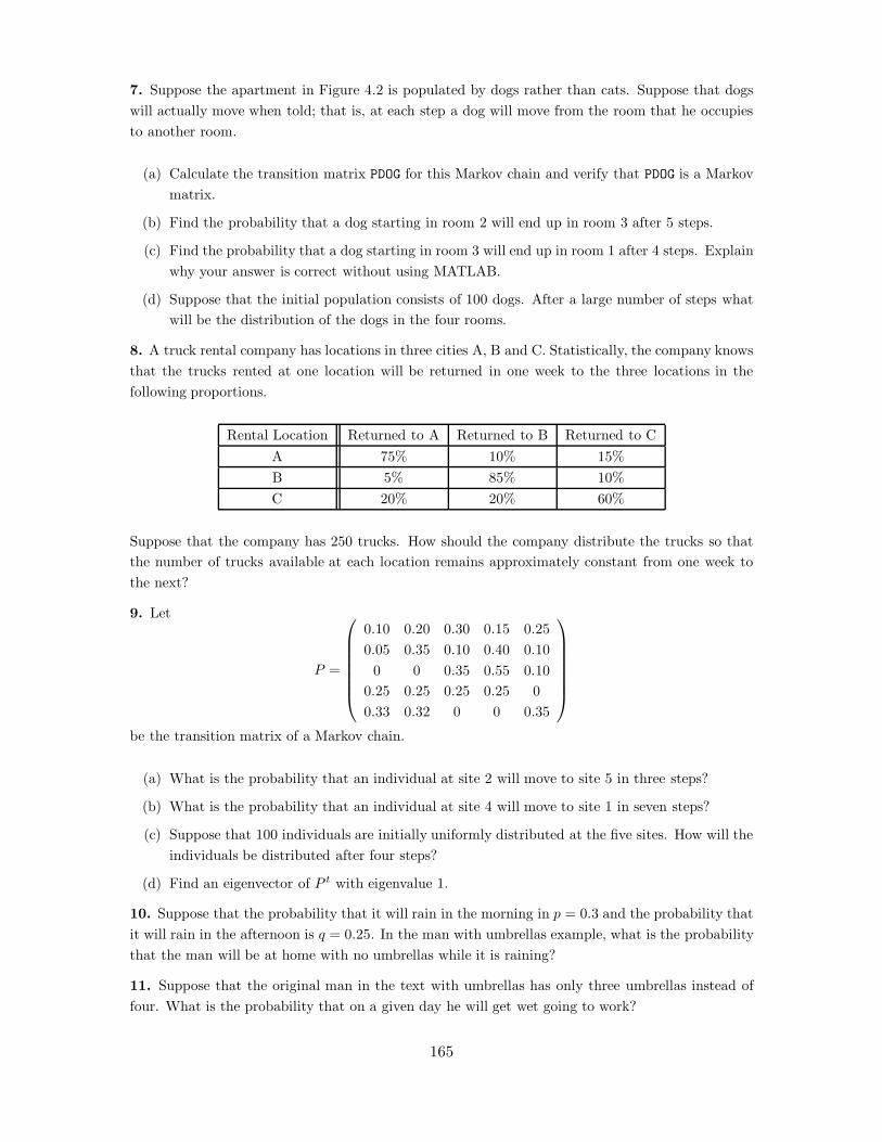
7. Suppose the apartment in Figure 4.2 is populated by dogs rather than cats. Suppose that dogswill actually move when told; that is, at each step a dog will move from the room that he occupiesto another room.

(a) Calculate the transition matrix PDOG for this Markov chain and verify that PDOG is a Markovmatrix.

(b) Find the probability that a dog starting in room 2 will end up in room 3 after 5 steps.

(c) Find the probability that a dog starting in room 3 will end up in room 1 after 4 steps. Explainwhy your answer is correct without using MATLAB.

(d) Suppose that the initial population consists of 100 dogs. After a large number of steps whatwill be the distribution of the dogs in the four rooms.

8. A truck rental company has locations in three cities A, B and C. Statistically, the company knowsthat the trucks rented at one location will be returned in one week to the three locations in thefollowing proportions.

Rental Location Returned to A Returned to B Returned to CA 75% 10% 15%B 5% 85% 10%C 20% 20% 60%

Suppose that the company has 250 trucks. How should the company distribute the trucks so thatthe number of trucks available at each location remains approximately constant from one week tothe next?

9. Let

P =

!

""""""#

0.10 0.20 0.30 0.15 0.250.05 0.35 0.10 0.40 0.100 0 0.35 0.55 0.10

0.25 0.25 0.25 0.25 00.33 0.32 0 0 0.35

$

%%%%%%&

be the transition matrix of a Markov chain.

(a) What is the probability that an individual at site 2 will move to site 5 in three steps?

(b) What is the probability that an individual at site 4 will move to site 1 in seven steps?

(c) Suppose that 100 individuals are initially uniformly distributed at the five sites. How will theindividuals be distributed after four steps?

(d) Find an eigenvector of P t with eigenvalue 1.

10. Suppose that the probability that it will rain in the morning in p = 0.3 and the probability thatit will rain in the afternoon is q = 0.25. In the man with umbrellas example, what is the probabilitythat the man will be at home with no umbrellas while it is raining?

11. Suppose that the original man in the text with umbrellas has only three umbrellas instead offour. What is the probability that on a given day he will get wet going to work?

165

4.6 Appendix: Existence of Determinants

The purpose of this appendix is to verify the inductive definition of determinant (4.1.9). We havealready shown that if a determinant function exists, then it is unique. We also know that thedeterminant function exists for 1 " 1 matrices. So we assume by induction that the determinantfunction exists for (n!1)"(n!1) matrices and prove that the inductive definition gives a determinantfunction for n" n matrices.

Recall that Aij is the cofactor matrix obtained from A by deleting the ith row and jth column— so Aij is an (n! 1)" (n ! 1) matrix. The inductive definition is:

D(A) = a11 det(A11)! a12 det(A12) + · · ·+ (!1)n+1a1n det(A1n).

We use the notation D(A) to remind us that we have not yet verified that this definition satisfiesproperties (a)-(c) of Definition 4.1.1. In this appendix we verify these properties after assuming thatthe inductive definition satisfies properties (a)-(c) for (n ! 1) " (n ! 1) matrices. For emphasis, weuse the notation det to indicate the determinant of square matrices of size less than n.

Property (a) is easily verified for D(A) since if A is lower triangular, then

D(A) = a11 det(A11) = a11a22 · · ·ann

by induction.

Before verifying that D satisfies properties (b) and (c) of a determinant, we prove:

Lemma 4.6.1. Let E be a elementary row matrix and let B be any n" n matrix. Then

D(EB) = D(E)D(B) (4.6.1)

Proof: We verify (4.6.1) for each of the three types of elementary row operations.

(I) Suppose that E multiplies the ith row by a nonzero scalar c. If i > 1, then the cofactor matrix(EA)1j is obtained from the cofactor matrix A1j by multiplying the (i!1)st row by c. By induction,det(EA)1j = c det(A1j) and D(EA) = cD(A). On the other hand, D(E) = det(E11) = c. So (4.6.1)is verified in this instance. If i = 1, then the 1st row of EA is (ca11, . . . , ca1n) from which it is easyto verify (4.6.1).

(II) Next suppose that E adds a multiple c of the ith row to the jth row. We note that D(E) = 1.When j > 1 then D(E) = det(E11) = 1 by induction. When j = 1 then D(E) = det(E11) ±c det(E1i) = det(In#1) ± c det(E1i). But E1i is strictly upper triangular and det(E1i) = 0. ThusD(E) = 1.

If i > 1 and j > 1, then the result D(EA) = D(A) = D(E)D(A) follows by induction.

If i = 1, then

D(EB) = b11 det((EB)11) + · · ·+ (!1)n+1b1n det((EB)1n)

= D(B) + cD(C)

166

where the 1st and ith row of C are equal.

If j = 1, then

D(EB) = (b11 + cbi1) det(B11) + · · ·+ (!1)n+1(b1n + cbin) det(B1n)

=1b11 det(B11) + · · ·+ (!1)n+1b1n det(B1n)

2+

c1bi1 det(B11) + · · ·+ (!1)n+1bi1 det(B1n)

2

= D(B) + cD(C)

where the 1st and ith row of C are equal.

The hardest part of this proof is a calculation that shows that if the 1st and ith rows of C areequal, then D(C) = 0. By induction, we can swap the ith row with the 2nd. Hence we need onlyverify this fact when i = 2.

(III) E is the matrix that swaps two rows.

As we saw earlier (4.1.4), E is the product of four matrices of types (I) and (II). It follows thatD(E) = !1 and D(EA) = !D(A) = D(E)D(A).

We now verify that when the 1st and 2nd rows of an n" n matrix C are equal, then D(C) = 0.This is a tedious calculation that requires some facility with indexes and summations. Rather thando this proof for general n, we present the proof for n = 4. This case contains all of the ideas of thegeneral proof.

We begin with the definition of D(C)

D(C) = c11 det

!

"#c22 c23 c24

c32 c33 c34

c42 c43 c44

$

%&! c12 det

!

"#c21 c23 c24

c31 c33 c34

c41 c43 c44

$

%& +

c13 det

!

"#c21 c22 c24

c31 c32 c34

c41 c42 c44

$

%&! c14 det

!

"#c21 c22 c23

c31 c32 c33

c41 c42 c43

$

%& .

Next we expand each of the four 3" 3 matrices along their 1st rows, obtaining

D(C) = c11

'c22 det

'c33 c34

c43 c44

(! c23 det

'c32 c34

c42 c44

(+ c24 det

'c32 c33

c42 c43

((

!c12

'c21 det

'c33 c34

c43 c44

(! c23 det

'c31 c34

c41 c44

(+ c24 det

'c31 c33

c41 c43

((

+c13

'c21 det

'c32 c34

c42 c44

(! c22 det

'c31 c34

c41 c44

(+ c24 det

'c31 c32

c41 c42

((

!c14

'c21 det

'c32 c33

c42 c43

(! c22 det

'c31 c33

c41 c43

(+ c23 det

'c31 c32

c41 c42

((

167

Combining the 2" 2 determinants leads to:

D(C) = (c11c22 ! c12c21) det

'c33 c34

c43 c44

(+ (c11c24 ! c14c21) det

'c32 c33

c42 c43

(

+(c12c23 ! c13c22) det

'c31 c34

c41 c44

(+ (c13c21 ! c11c23) det

'c32 c34

c42 c44

(

+(c13c24 ! c14c23) det

'c31 c32

c41 c42

(+ (c14c22 ! c12c24) det

'c31 c33

c41 c43

(

Supposing thatc21 = c11 c22 = c12 c23 = c13 c24 = c14

it is now easy to check that D(C) = 0.

We now return to verifying that D(A) satisfies properties (b) and (c) of being a determinant.We begin by showing that D(A) = 0 if A has a row that is identically zero. Suppose that the zerorow is the ith row and let E be the matrix that multiplies the ith row of A by c. Then EA = A.Using (4.6.1) we see that

D(A) = D(EA) = D(E)D(A) = cD(A),

which implies that D(A) = 0 since c is arbitrary.

Next we prove that D(A) = 0 when A is singular. Using row reduction we can write

A = Es · · ·E1R

where the Ej are elementary row matrices and R is in reduced echelon form. Since A is singular,the last row of R is identically zero. Hence D(R) = 0 and (4.6.1) implies that D(A) = 0.

We now verify property (b). Suppose that A is singular; we show that D(At) = D(A) = 0. Sincethe row rank of A equals the column rank of A, it follows that At is singular when A is singular.Next assume that A is nonsingular. Then A is row equivalent to In and we can write

A = Es · · ·E1, (4.6.2)

where the Ej are elementary row matrices. Since

At = Et1 · · ·Et

s

and D(E) = D(Et), property (b) follows.

We now verify property (c): D(AB) = D(A)D(B). Recall that A is singular if and only ifthere exists a nonzero vector v such that Av = 0. Now if A is singular, then so is At. Therefore(AB)t = BtAt is also singular. To verify this point, let w be the nonzero vector such that Atw = 0.Then BtAtw = 0. Thus AB is singular since (AB)t is singular. Thus D(AB) = 0 = D(A)D(B)when A is singular. Suppose now that A is nonsingular. It follows that

AB = Es · · ·E1B.

Using (4.6.1) we see that

D(AB) = D(Es) · · ·D(E1)D(B) = D(Es · · ·E1)D(B) = D(A)D(B),

as desired. We have now completed the proof that a determinant function exists.

168

Chapter 5

Vector Spaces

In Chapter 2 we discussed how to solve systems of m linear equations in n unknowns.We found that solutions of these equations are vectors (x1, . . . , xn) $ Rn. In Chapter 3we discussed how the notation of matrices and matrix multiplication drastically simplifiesthe presentation of linear systems and how matrix multiplication leads to linear mappings.We also discussed briefly how linear mappings lead to methods for solving linear systems— superposition, eigenvectors, inverses. These chapters have provided an introduction tomany of the ideas of linear algebra and now we begin the task of formalizing these ideas.

Sets having the two operations of vector addition and scalar multiplication are calledvector spaces . This concept is introduced in Section 5.1 along with the two primary exam-ples — the set Rn in which solutions to systems of linear equations sit and the set C1 ofdi"erentiable functions in which solutions to systems of ordinary di"erential equations sit.Solutions to systems of homogeneous linear equations form subspaces of Rn and solutionsof systems of linear di"erential equations form subspaces of C1. These issues are discussedin Sections 5.1 and 5.2.

When we solve a homogeneous system of equations, we write every solution as a su-perposition of a finite number of specific solutions. Abstracting this process is one of themain points of this chapter. Specifically, we show that every vector in many commonlyoccurring vector spaces (in particular, the subspaces of solutions) can be written as a linearcombination (superposition) of a few solutions. The minimum number of solutions neededis called the dimension of that vector space. Sets of vectors that generate all solutions bysuperposition and that consist of that minimum number of vectors are called bases . Theseideas are discussed in detail in Sections 5.3–5.5. The proof of the main theorem (Theo-rem 5.5.3), which gives a computable method for determining when a set is a basis, is givenin Section 5.6. This proof may be omitted on a first reading, but the statement of thetheorem is most important and must be understood.

169

5.1 Vector Spaces and Subspaces

Vector spaces abstract the arithmetic properties of addition and scalar multiplication ofvectors. In Rn we know how to add vectors and to multiply vectors by scalars. Indeed,it is straightforward to verify that each of the eight properties listed in Table 5.1 is validfor vectors in V = Rn. Remarkably, sets that satisfy these eight properties have much incommon with Rn. So we define:

Definition 5.1.1. Let V be a set having the two operations of addition and scalar multi-plication. Then V is a vector space if the eight properties listed in Table 5.1.1 hold. Theelements of a vector space are called vectors.

Table 5.1: Properties of Vector Spaces: suppose u, v, w $ V and r, s $ R.

(A1) Addition is commutative v + w = w + v

(A2) Addition is associative (u + v) + w = u + (v + w)(A3) Additive identity 0 exists v + 0 = v

(A4) Additive inverse "v exists v + ("v) = 0(M1) Multiplication is associative (rs)v = r(sv)(M2) Multiplicative identity exists 1v = v

(D1) Distributive law for scalars (r + s)v = rv + sv

(D2) Distributive law for vectors r(v + w) = rv + rw

The vector 0 mentioned in (A3) in Table 5.1 is called the zero vector.

When we say that a vector space V has the two operations of addition and scalarmultiplication we mean that the sum of two vectors in V is again a vector in V and thescalar product of a vector with a number is again a vector in V . These two properties arecalled closure under addition and closure under scalar multiplication.

In this discussion we focus on just two types of vector spaces: Rn and function spaces.The reason that we make this choice is that solutions to linear equations are vectors in Rn

while solutions to linear systems of di"erential equations are vectors of functions.

An Example of a Function Space

For example, let F denote the set of all functions f : R & R. Note that functions likef1(t) = t2 " 2t + 7 and f2(t) = sin t are in F since they are defined for all real numbers t,but that functions like g1(t) = 1

t and g2(t) = tan t are not in F since they are not definedfor all t.

170

We can add two functions f and g by defining the function f + g to be:

(f + g)(t) = f(t) + g(t).

We can also multiply a function f by a scalar c $ R by defining the function cf to be:

(cf)(t) = cf(t).

With these operations of addition and scalar multiplication, F is a vector space; that is, Fsatisfies the eight vector space properties in Table 5.1. More precisely:

(A3) Define the zero function O by

O(t) = 0 for all t $ R.

For every x in F the function O satisfies:

(x + O)(t) = x(t) + O(t) = x(t) + 0 = x(t).

Therefore, x + O = x and O is the additive identity in F .

(A4) Let x be a function in F and define y(t) = "x(t). Then y is also a function in F , and

(x + y)(t) = x(t) + y(t) = x(t) + ("x(t)) = 0 = O(t).

Thus, x has the additive inverse "x.

After these comments it is straightforward to verify that the remaining six properties inTable 5.1 are satisfied by functions in F .

Sets that are not Vector Spaces

It is worth considering how closure under vector addition and scalar multiplication can fail.Consider the following three examples.

(i) Let V1 be the set that consists of just the x and y axes in the plane. Since (1, 0) and(0, 1) are in V1 but

(1, 0) + (0, 1) = (1, 1)

is not in V1, we see that V1 is not closed under vector addition. On the other hand,V1 is closed under scalar multiplication.

(ii) Let V2 be the set of all vectors (k, ') $ R2 where k and ' are integers. The set V2 isclosed under addition but not under scalar multiplication since 1

2(1, 0) = (12 , 0) is not

in V2.

(iii) Let V3 = [1, 2] be the closed interval in R. The set V3 is neither closed under addition(1 + 1.5 = 2.5 %$ V3) nor under scalar multiplication (4 · 1.5 = 6 %$ V3). Hence the setV3 is not closed under vector addition and not closed under scalar multiplication.

171

Subspaces

Definition 5.1.2. Let V be a vector space. A nonempty subset W ' V is a subspace if W

is a vector space using the operations of addition and scalar multiplication defined on V .

Note that in order for a subset W of a vector space V to be a subspace it must be closedunder addition and closed under scalar multiplication. That is, suppose w1, w2 $ W andr $ R. Then

(i) w1 + w2 $ W , and

(ii) rw1 $ W .

The x-axis and the xz-plane are examples of subsets of R3 that are closed under additionand closed under scalar multiplication. Every vector on the x-axis has the form (a, 0, 0) $R3. The sum of two vectors (a, 0, 0) and (b, 0, 0) on the x-axis is (a + b, 0, 0) which is alsoon the x-axis. The x-axis is also closed under scalar multiplication as r(a, 0, 0) = (ra, 0, 0),and the x-axis is a subspace of R3. Similarly, every vector in the xz-plane in R3 has theform (a1, 0, a3). As in the case of the x-axis, it is easy to verify that this set of vectors isclosed under addition and scalar multiplication. Thus, the xz-plane is also a subspace ofR3.

In Theorem 5.1.4 we show that every subset of a vector space that is closed underaddition and scalar multiplication is a subspace. To verify this statement, we need thefollowing lemma in which some special notation is used. Typically, we use the same notation0 to denote the real number zero and the zero vector. In the following lemma it is convenientto distinguish the two di"erent uses of 0, and we write the zero vector in boldface.

Lemma 5.1.3. Let V be a vector space, and let 0 $ V be the zero vector. Then

0v = 0 and ("1)v = "v

for every vector in v $ V .

Proof: Let v be a vector in V and use (D1) to compute

0v + 0v = (0 + 0)v = 0v.

By (A4) the vector 0v has an additive inverse "0v. Adding "0v to both sides yields

(0v + 0v) + ("0v) = 0v + ("0v) = 0.

Associativity of addition (A2) now implies

0v + (0v + ("0v)) = 0.

172

A second application of (A4) implies that

0v + 0 = 0

and (A3) implies that 0v = 0.

Next, we show that the additive inverse "v of a vector v is unique. That is, if v +a = 0,then a = "v.

Before beginning the proof, note that commutativity of addition (A1) together with(A3) implies that 0 + v = v. Similarly, (A1) and (A4) imply that "v + v = 0.

To prove uniqueness of additive inverses, add "v to both sides of the equation v +a = 0yielding

"v + (v + a) = "v + 0.

Properties (A2) and (A3) imply

("v + v) + a = "v.

But("v + v) + a = 0 + a = a.

Therefore a = "v, as claimed.

To verify that ("1)v = "v, we show that ("1)v is the additive inverse of v. Using (M1),(D1), and the fact that 0v = 0, calculate

v + ("1)v = 1v + ("1)v = (1 " 1)v = 0v = 0.

Thus, ("1)v is the additive inverse of v and must equal "v, as claimed.

Theorem 5.1.4. Let W be a subset of the vector space V . If W is closed under additionand closed under scalar multiplication, then W is a subspace.

Proof: We have to show that W is a vector space using the operations of addition andscalar multiplication defined on V . That is, we need to verify that the eight propertieslisted in Table 5.1 are satisfied. Note that properties (A1), (A2), (M1), (M2), (D1), and(D2) are valid for vectors in W since they are valid for vectors in V .

It remains to verify (A3) and (A4). Let w $ W be any vector. Since W is closed underscalar multiplication, it follows that 0w and ("1)w are in W . Lemma 5.1.3 states that0w = 0 and ("1)w = "w; it follows that 0 and "w are in W . Hence, properties (A3) and(A4) are valid for vectors in W , since they are valid for vectors in V .

173

Examples of Subspaces of Rn

Example 5.1.5. (a) Let V be a vector space. Then the subsets V and {0} are alwayssubspaces of V . A subspace W ' V is proper if W %= 0 and W %= V .

(b) Lines through the origin are subspaces of Rn. Let w $ Rn be a nonzerovector and let W = {rw : r $ R}. The set W is closed under addition and scalarmultiplication and is a subspace of Rn by Theorem 5.1.4. The subspace W is just aline through the origin in Rn, since the vector rw points in the same direction as w

when r > 0 and the exact opposite direction when r < 0.

(c) Planes containing the origin are subspaces of R3. To verify this point, let P be aplane through the origin and let N be a vector perpendicular to P . Then P consists ofall vectors v $ R3 perpendicular to N ; using the dot-product (see Chapter 2, (2.2.3))we recall that such vectors satisfy the linear equation N ·v = 0. By superposition, theset of all solutions to this equation is closed under addition and scalar multiplicationand is therefore a subspace by Theorem 5.1.4.

In a sense that will be made precise all subspaces of Rn can be written as the span of afinite number of vectors generalizing Example 5.1.5(b) or as solutions to a system of linearequations generalizing Example 5.1.5(c).

Examples of Subspaces of the Function Space F

Let P be the set of all polynomials in F . The sum of two polynomials is a polynomial andthe scalar multiple of a polynomial is a polynomial. Thus, P is closed under addition andscalar multiplication, and P is a subspace of F .

As a second example of a subspace of F , let C1 be the set of all continuously di"erentiablefunctions u : R & R. A function u is in C1 if u and u! exist and are continuous for all t $ R.Examples of functions in C1 are:

(i) Every polynomial p(t) = amtm + am#1tm#1 + · · ·+ a1t + a0 is in C1.

(ii) The function u(t) = e"t is in C1 for each constant & $ R.

(iii) The trigonometric functions u(t) = sin(&t) and v(t) = cos(&t) are in C1 for eachconstant & $ R.

(iv) u(t) = t7/3 is twice di"erentiable everywhere and is in C1.

Equally there are many commonly used functions that are not in C1. Examples include:

174

(i) u(t) = 1t#5 is neither defined nor continuous at t = 5.

(ii) u(t) = |t| is not di"erentiable (at t = 0).

(iii) u(t) = csc(t) is neither defined nor continuous at t = k( for any integer k.

The subset C1 ' F is a subspace and hence a vector space. The reason is simple. If x(t)and y(t) are continuously di"erentiable, then

d

dt(x + y) =

dx

dt+

dy

dt.

Hence x + y is di"erentiable and is in C1 and C1 is closed under addition. Similarly, C1 isclosed under scalar multiplication. Let r $ R and let x $ C1. Then

d

dt(rx)(t) = r

dx

dt(t).

Hence rx is di"erentiable and is in C1.

The Vector Space (C1)n

Another example of a vector space that combines the features of both Rn and C1 is (C1)n.Vectors u $ (C1)n have the form

u(t) = (u1(t), . . . , un(t)),

where each coordinate function uj(t) $ C1. Addition and scalar multiplication in (C1)n aredefined coordinatewise — just like addition and scalar multiplication in Rn. That is, letu, v be in (C1)n and let r be in R, then

(u + v)(t) = (u1(t) + v1(t), . . . , un(t) + vn(t))

(ru)(t) = (ru1(t), . . . , run(t)).

The set (C1)n satisfies the eight properties of vector spaces and is a vector space. Solutionsto systems of n linear ordinary di"erential equations are vectors in (C1)n.

Hand Exercises

1. Verify that the set V1 consisting of all scalar multiples of (1,!1,!2) is a subspace of R3.

2. Let V2 be the set of all 2" 3 matrices. Verify that V2 is a vector space.

3. Let

A =

'1 1 01 !1 1

(.

Let V3 be the set of vectors x % R3 such that Ax = 0. Verify that V3 is a subspace of R3. CompareV1 with V3.

175

In Exercises 4 – 10 you are given a vector space V and a subset W . For each pair, decide whetheror not W is a subspace of V .

4. V = R3 and W consists of vectors in R3 that have a 0 in their first component.

5. V = R3 and W consists of vectors in R3 that have a 1 in their first component.

6. V = R2 and W consists of vectors in R2 for which the sum of the components is 1.

7. V = R2 and W consists of vectors in R2 for which the sum of the components is 0.

8. V = C1 and W consists of functions x(t) % C1 satisfying3 4#2 x(t)dt = 0.

9. V = C1 and W consists of functions x(t) % C1 satisfying x(1) = 0.

10. V = C1 and W consists of functions x(t) % C1 satisfying x(1) = 1.

In Exercises 11 – 15 which of the sets S are subspaces?

11. S = {(a, b, c) % R3 : a ' 0, b ' 0, c ' 0}.

12. S = {(x1, x2, x3) % R3 : a1x1 + a2x2 + a3x3 = 0 where a1, a2, a3 % R are fixed}.

13. S = {(x, y) % R2 : (x, y) is on the line through (1, 1) with slope 1}.

14. S = {x % R2 : Ax = 0} where A is a 3" 2 matrix.

15. S = {x % R2 : Ax = b} where A is a 3" 2 matrix and b % R3 is a fixed nonzero vector.

16. Let V be a vector space and let W1 and W2 be subspaces. Show that the intersection W1 0W2

is also a subspace of V .

17. For which scalars a, b, c do the solutions to the equation

ax + by = c

form a subspace of R2?

18. For which scalars a, b, c, d do the solutions to the equation

ax + by + cz = d

form a subspace of R3?

176

5.2 Construction of Subspaces

The principle of superposition shows that the set of all solutions to a homogeneous system of linearequations is closed under addition and scalar multiplication and is a subspace. Indeed, there aretwo ways to describe subspaces: first as solutions to linear systems, and second as the span of a setof vectors. We shall see that solving a homogeneous linear system of equations just means writingthe solution set as the span of a finite set of vectors.

Solutions to Homogeneous Systems Form Subspaces

Definition 5.2.1. Let A be an m " n matrix. The null space of A is the set of solutions to thehomogeneous system of linear equations

Ax = 0. (5.2.1)

Lemma 5.2.2. Let A be an m " n matrix. Then the null space of A is a subspace of Rn.

Proof: Suppose that x and y are solutions to (5.2.1). Then

A(x + y) = Ax + Ay = 0 + 0 = 0;

so x + y is a solution of (5.2.1). Similarly, for r % R

A(rx) = rAx = r0 = 0;

so rx is a solution of (5.2.1). Thus, x + y and rx are in the null space of A, and the null space isclosed under addition and scalar multiplication. So Theorem 5.1.4 implies that the null space is asubspace of the vector space Rn.

Writing Solution Subspaces as a Span

The way we solve homogeneous systems of equations gives a second method for defining subspaces.For example, consider the system

Ax = 0,

where

A =

'2 1 4 0!1 0 2 1

(.

The matrix A is row equivalent to the reduced echelon form matrix

E =

'1 0 !2 !10 1 8 2

(.

Therefore x = (x1, x2, x3, x4) is a solution of Ex = 0 if and only if x1 = 2x3+x4 and x2 = !8x3!2x4.It follows that every solution of Ex = 0 can be written as:

x = x3

!

"""#

2!8

10

$

%%%&+ x4

!

"""#

1!2

01

$

%%%&.

177

Since row operations do not change the set of solutions, it follows that every solution of Ax = 0has this form. We have also shown that every solution is generated by two vectors by use of vectoraddition and scalar multiplication. We say that this subspace is spanned by the two vectors

!

"""#

2!8

10

$

%%%&and

!

"""#

1!2

01

$

%%%&.

For example, a calculation verifies that the vector!

"""#

1!10

2!3

$

%%%&

is also a solution of Ax = 0 since!

"""#

1!10

2!3

$

%%%& = 2

!

"""#

2!8

10

$

%%%&! 3

!

"""#

1!2

01

$

%%%& . (5.2.2)

Spans

Let v1, . . . , vk be a set of vectors in a vector space V . A vector v % V is a linear combination ofv1, . . . , vk if

v = r1v1 + · · ·+ rkvk

for some scalars r1, . . . , rk.

Definition 5.2.3. The set of all linear combinations of the vectors v1, . . . , vk in a vector space V

is the span of v1, . . . , vk and is denoted by span{v1, . . . , vk}.

For example, the vector on the left hand side in (5.2.2) is a linear combination of the two vectorson the right hand side.

The simplest example of a span is Rn itself. Let vj = ej where ej % Rn is the vector with a 1 inthe jth coordinate and 0 in all other coordinates. Then every vector x = (x1, . . . , xn) % Rn can bewritten as

x = x1e1 + · · ·+ xnen.

It follows thatRn = span{e1, . . . , en}.

Similarly, the set span{e1, e3} 1 R3 is just the x1x3-plane, since vectors in this span are

x1e1 + x3e3 = x1(1, 0, 0) + x3(0, 0, 1) = (x1, 0, x3).

Proposition 5.2.4. Let V be a vector space and let w1, . . . , wk % V . Then W = span{w1, . . . , wk} 1V is a subspace.

178

Proof: Suppose x, y %W . Then

x = r1w1 + · · ·+ rkwk

y = s1w1 + · · ·+ skwk

for some scalars r1, . . . , rk and s1, . . . , sk. It follows that

x + y = (r1 + s1)w1 + · · ·+ (rk + sk)wk

andrx = (rr1)w1 + · · ·+ (rrk)wk

are both in span{w1, . . . , wk}. Hence W 1 V is closed under addition and scalar multiplication, andis a subspace by Theorem 5.1.4.

For example, letv = (2, 1, 0) and w = (1, 1, 1) (5.2.3)

be vectors in R3. Then linear combinations of the vectors v and w have the form

$v + %w = (2$+ %,$+ %, %)

for real numbers $ and %. Note that every one of these vectors is a solution to the linear equation

x1 ! 2x2 + x3 = 0, (5.2.4)

that is, the 1st coordinate minus twice the 2nd coordinate plus the 3rd coordinate equals zero.Moreover, you may verify that every solution of (5.2.4) is a linear combination of the vectors v andw in (5.2.3). Thus, the set of solutions to the homogeneous linear equation (5.2.4) is a subspace,and that subspace can be written as the span of all linear combinations of the vectors v and w.

In this language we see that the process of solving a homogeneous system of linear equations isjust the process of finding a set of vectors that span the subspace of all solutions. Indeed, we cannow restate Theorem 2.4.6 of Chapter 2. Recall that a matrix A has rank # if it is row equivalentto a matrix in echelon form with # nonzero rows.

Proposition 5.2.5. Let A be an m" n matrix with rank #. Then the null space of A is the span ofn! # vectors.

We have now seen that there are two ways to describe subspaces — as solutions of homogeneoussystems of linear equations and as a span of a set of vectors, the spanning set. Much of linear algebrais concerned with determining how one goes from one description of a subspace to the other.

Hand Exercises

In Exercises 1 – 4 a single equation in three variables is given. For each equation write the subspaceof solutions in R3 as the span of two vectors in R3.

179

1. 4x! 2y + z = 0.

2. x! y + 3z = 0.

3. x + y + z = 0.

4. y = z.

In Exercises 5 – 8 each of the given matrices is in reduced echelon form. Write solutions of thecorresponding homogeneous system of linear equations as a span of vectors.

5. A =

!

"#1 2 0 1 00 0 1 4 00 0 0 0 1

$

%&.

6. B =

'1 3 0 50 0 1 2

(.

7. A =

'1 0 20 1 1

(.

8. B =

!

"#1 !1 0 5 0 00 0 1 2 0 20 0 0 0 1 2

$

%&.

9. Write a system of two linear equations of the form Ax = 0 where A is a 2 " 4 matrix whosesubspace of solutions in R4 is the span of the two vectors

v1 =

!

"""#

1!1

00

$

%%%& and v2 =

!

"""#

001!1

$

%%%& .

10. Write the matrix A =

'2 2!3 0

(as a linear combination of the matrices

B =

'1 10 0

(and C =

'0 01 0

(.

11. Is (2, 20, 0) in the span of w1 = (1, 1, 3) and w2 = (1, 4, 2)? Answer this question by settingup a system of linear equations and solving that system by row reducing the associated augmentedmatrix.

In Exercises 12 – 15 let W 1 C1 be the subspace spanned by the two polynomials x1(t) = 1 andx2(t) = t2. For the given function y(t) decide whether or not y(t) is an element of W . Furthermore,if y(t) %W , determine whether the set {y(t), x2(t)} is a spanning set for W .

12. y(t) = 1! t2,

13. y(t) = t4,

180

14. y(t) = sin t,

15. y(t) = 0.5t2

16. Let W 1 R4 be the subspace that is spanned by the vectors

w1 = (!1, 2, 1, 5) and w2 = (2, 1, 3, 0).

Find a linear system of two equations such that W = span{w1, w2} is the set of solutions of thissystem.

17. Let V be a vector space and let v % V be a nonzero vector. Show that

span{v, v} = span{v}.

18. Let V be a vector space and let v, w % V be vectors. Show that

span{v, w} = span{v, w, v + 3w}.

19. Let W = span{w1, . . . , wk} be a subspace of the vector space V and let wk+1 % W be anothervector. Prove that W = span{w1, . . . , wk+1}.

20. Let Ax = b be a system of m linear equations in n unknowns, and let r = rank(A) ands = rank(A|b). Suppose that this system has a unique solution. What can you say about therelative magnitudes of m, n, r, s?

5.3 Spanning Sets and MATLAB

In this section we discuss:

• how to find a spanning set for the subspace of solutions to a homogeneous system of linearequations using the MATLAB command null, and

• how to determine when a vector is in the subspace spanned by a set of vectors using theMATLAB command rref.

Spanning Sets for Homogeneous Linear Equations

In Chapter 2 we saw how to use Gaussian elimination, back substitution, and MATLAB to computesolutions to a system of linear equations. For systems of homogeneous equations, MATLAB providesa command to find a spanning set for the subspace of solutions. That command is null. For example,if we type

A = [2 1 4 0; -1 0 2 1]

B = null(A)

then we obtain

181

B =

0.4830 0

-0.4140 0.8729

-0.1380 -0.2182

0.7591 0.4364

The two columns of the matrix B span the set of solutions of the equation Ax = 0. In particular,the vector (2,!8, 1, 0) is a solution to Ax = 0 and is therefore a linear combination of the columnvectors of B. Indeed, type

4.1404*B(:,1)-7.2012*B(:,2)

and observe that this linear combination is the desired one.

Next we describe how to find the coe!cients 4.1404 and -7.2012 by showing that these coe!-cients themselves are solutions to another system of linear equations.

When is a Vector in a Span?

Let w1, . . . , wk and v be vectors in Rn. We now describe a method that allows us to decide whetherv is in span{w1, . . . , wk}. To answer this question one has to solve a system of n linear equations ink unknowns. The unknowns correspond to the coe!cients in the linear combination of the vectorsw1, . . . , wk that gives v.

Let us be more precise. The vector v is in span{w1, . . . , wk} if and only if there are constantsr1, . . . , rk such that the equation

r1w1 + · · ·+ rkwk = v (5.3.1)

is valid. Define the n" k matrix A as the one having w1, . . . , wk as its columns; that is,

A = (w1| · · · |wk). (5.3.2)

Let r be the k-vector

r =

!

""#

r1

...rk

$

%%& .

Then we may rewrite equation (5.3.1) asAr = v. (5.3.3)

To summarize:

Lemma 5.3.1. Let w1, . . . , wk and v be vectors in Rn. Then v is in span{w1, . . . , wk} if and onlyif the system of linear equations (5.3.3) has a solution where A is the n " k defined in (5.3.2).

To solve (5.3.3) we row reduce the augmented matrix (A|v). For example, is v = (2, 1) in thespan of w1 = (1, 1) and w2 = (1,!1)? That is, do there exist scalars r1, r2 such that

r1 (1, 1) + r2 (1, !1) = (2, 1)?

182

As noted, we can rewrite this equation as'

1 11 !1

((r1, r2) = (2, 1) .

We can solve this equation by row reducing the augmented matrix'

1 1 21 !1 1

(

to obtain '1 0 3

2

0 1 12

(.

So v = 32w1 + 1

2w2.

Row reduction to reduced echelon form has been preprogrammed in the MATLAB commandrref. Consider the following example. Let

w1 = (2, 0,!1, 4) and w2 = (2,!1, 0, 2) (5.3.4)

and ask the question whether v = (!2, 4,!3, 4) is in span{w1, w2}.

In MATLAB load the matrix A having w1 and w2 as its columns and the vector v by typinge5 3 5

A =

!

"""#

2 20 !1!1 0

4 2

$

%%%& and v =

!

"""#

!24!3

4

$

%%%& .

We can solve the system of equations using MATLAB. First, form the augmented matrix by typing

aug = [A v]

Then solve the system by typing rref(aug) to obtain

ans =

1 0 3

0 1 -4

0 0 0

0 0 0

It follows that (r1, r2) = (3,!4) is a solution and v = 3w1 ! 4w2.

Now we change the 4th entry in v slightly by typing v(4) = 4.01. There is no solution to thesystem of equations

Ar =

!

"""#

!24!3

4.01

$

%%%&

as we now show. Type

183

aug = [A v]

rref(aug)

which yields

ans =

1 0 0

0 1 0

0 0 1

0 0 0

This matrix corresponds to an inconsistent system; thus v is no longer in the span of w1 and w2.

Computer Exercises

In Exercises 1 – 3 use the null command in MATLAB to find all the solutions of the linear systemof equations Ax = 0.

1.

A =

'!4 0 !4 3!4 1 !1 1

(

2.

A =

!

"#1 21 03 !2

$

%&

3.

A =

'1 1 2!1 2 !1

(.

4. Use the null command in MATLAB to verify your answers to Exercises 5 and 6.

5. Use row reduction to find the solutions to Ax = 0 where A is given in (1). Does your answeragree with the MATLAB answer using null? If not, explain why.

In Exercises 6 – 8 let W 1 R5 be the subspace spanned by the vectors

w1 = (2, 0,!1, 3, 4), w2 = (1, 0, 0,!1, 2), w3 = (0, 1, 0, 0,!1).

Use MATLAB to decide whether the given vectors are elements of W .

6. v1 = (2, 1,!2, 8, 3).

7. v2 = (!1, 12, 3,!14,!1).

8. v3 = (!1, 12, 3,!14,!14).

184

5.4 Linear Dependence and Linear Independence

An important question in linear algebra concerns finding spanning sets for subspaces having thesmallest number of vectors. Let w1, . . . , wk be vectors in a vector space V and let W = span{w1, . . . , wk}.Suppose that W is generated by a subset of these k vectors. Indeed, suppose that the kth vector isredundant in the sense that W = span{w1, . . . , wk#1}. Since wk % W , this is possible only if wk isa linear combination of the k ! 1 vectors w1, . . . , wk#1; that is, only if

wk = r1w1 + · · ·+ rk#1wk#1. (5.4.1)

Definition 5.4.1. Let w1, . . . , wk be vectors in the vector space V . The set {w1, . . . , wk} is linearlydependent if one of the vectors wj can be written as a linear combination of the remaining k ! 1vectors.

Note that when k = 1, the phrase ‘{w1} is linearly dependent’ means that w1 = 0.

If we set rk = !1, then we may rewrite (5.4.1) as

r1w1 + · · ·+ rk#1wk#1 + rkwk = 0.

It follows that:

Lemma 5.4.2. The set of vectors {w1, . . . , wk} is linearly dependent if and only if there exist scalarsr1, . . . , rk such that

(a) at least one of the rj is nonzero, and

(b) r1w1 + · · ·+ rkwk = 0.

For example, the vectors w1 = (2, 4, 7), w2 = (5, 1,!1), and w3 = (1,!7,!15) are linearlydependent since 2w1 !w2 + w3 = 0.

Definition 5.4.3. A set of k vectors {w1, . . . , wk} is linearly independent if none of the k vectorscan be written as a linear combination of the other k ! 1 vectors.

Since linear independence means not linearly dependent, Lemma 5.4.2 can be rewritten as:

Lemma 5.4.4. The set of vectors {w1, . . . , wk} is linearly independent if and only if whenever

r1w1 + · · ·+ rkwk = 0,

it follows thatr1 = r2 = · · · = rk = 0.

Let ej be the vector in Rn whose jth component is 1 and all of whose other components are 0.The set of vectors e1, . . . , en is the simplest example of a set of linearly independent vectors in Rn.We use Lemma 5.4.4 to verify independence by supposing that

r1e1 + · · ·+ rnen = 0.

A calculation shows that0 = r1e1 + · · ·+ rnen = (r1, . . . , rn).

It follows that each rj equals 0, and the vectors e1, . . . , en are linearly independent.

185

Deciding Linear Dependence and Linear Independence

Deciding whether a set of k vectors in Rn is linearly dependent or linearly independent is equivalentto solving a system of linear equations. Let w1, . . . , wk be vectors in Rn, and view these vectors ascolumn vectors. Let

A = (w1| · · · |wk) (5.4.2)

be the n" k matrix whose columns are the vectors wj . Then a vector

R =

!

""#

r1

...rk

$

%%&

is a solution to the system of equations AR = 0 precisely when

r1w1 + · · ·+ rkwk = 0. (5.4.3)

If there is a nonzero solution R to AR = 0, then the vectors {w1, . . . , wk} are linearly dependent; ifthe only solution to AR = 0 is R = 0, then the vectors are linearly independent.

The preceding discussion is summarized by:

Lemma 5.4.5. The vectors w1, . . . , wk in Rn are linearly dependent if the null space of the n " k

matrix A defined in (5.4.2) is nonzero and linearly independent if the null space of A is zero.

A Simple Example of Linear Independence with Two Vectors

The two vectors

w1 =

!

"""#

2!8

10

$

%%%&and w2 =

!

"""#

1!2

01

$

%%%&

are linearly independent. To see this suppose that r1w1 + r2w2 = 0. Using the components of w1

and w2 this equality is equivalent to the system of four equations

2r1 + r2 = 0, !8r1 ! 2r2 = 0, r1 = 0, and r2 = 0.

In particular, r1 = r2 = 0; hence w1 and w2 are linearly independent.

Using MATLAB to Decide Linear Dependence

Suppose that we want to determine whether or not the vectors

w1 =

!

""""""#

12!1

35

$

%%%%%%&w2 =

!

""""""#

!114!2

0

$

%%%%%%&w3 =

!

""""""#

11!1

312

$

%%%%%%&w4 =

!

""""""#

0431!2

$

%%%%%%&

are linearly dependent. After typing e5 4 4 in MATLAB, form the 5" 4 matrix A by typing

186

A = [w1 w2 w3 w4]

Determine whether there is a nonzero solution to AR = 0 by typing

null(A)

The response from MATLAB is

ans =

-0.7559

-0.3780

0.3780

0.3780

showing that there is a nonzero solution to AR = 0 and the vectors wj are linearly dependent.Indeed, this solution for R shows that we can solve for w1 in terms of w2, w3, w4. We can now askwhether or not w2, w3, w4 are linearly dependent. To answer this question form the matrix

B = [w2 w3 w4]

and type null(B) to obtain

ans =

Empty matrix: 3-by-0

showing that the only solution to BR = 0 is the zero solution R = 0. Thus, w2, w3, w4 are linearlyindependent. For these particular vectors, any three of the four are linearly independent.

Hand Exercises

1. Let w be a vector in the vector space V . Show that the sets of vectors {w, 0} and {w,!w} arelinearly dependent.

2. For which values of b are the vectors (1, b) and (3,!1) linearly independent?

3. Letu1 = (1,!1, 1) u2 = (2, 1,!2) u3 = (10, 2,!6).

Is the set {u1, u2, u3} linearly dependent or linearly independent?

4. For which values of b are the vectors (1, b, 2b) and (2, 1, 4) linearly independent?

5. Show that the polynomials p1(t) = 2+t, p2(t) = 1+t2, and p3(t) = t!t2 are linearly independentvectors in the vector space C1.

187

6. Show that the functions f1(t) = sin t, f2(t) = cos t, and f3(t) = cos4t + "

3

5are linearly dependent

vectors in C1.

7. Suppose that the three vectors u1, u2, u3 % Rn are linearly independent. Show that the set

{u1 + u2, u2 + u3, u3 + u1}

is also linearly independent.

Computer Exercises

In Exercises 8 – 8, determine whether the given sets of vectors are linearly independent or linearlydependent.

8.v1 = (2, 1, 3, 4) v2 = (!4, 2, 3, 1) v3 = (2, 9, 21, 22)

9.w1 = (1, 2, 3) w2 = (2, 1, 5) w3 = (!1, 2,!4) w4 = (0, 2,!1)

10.x1 = (3, 4, 1, 2, 5) x2 = (!1, 0, 3,!2, 1) x3 = (2, 4,!3, 0, 2)

11. Perform the following experiments.

(a) Use MATLAB to choose randomly three column vectors in R3. The MATLAB commands tochoose these vectors are:

y1 = rand(3,1)

y2 = rand(3,1)

y3 = rand(3,1)

Use the methods of this section to determine whether these vectors are linearly independentor linearly dependent.

(b) Now perform this exercise five times and record the number of times a linearly independentset of vectors is chosen and the number of times a linearly dependent set is chosen.

(c) Repeat the experiment in (b) — but this time randomly choose four vectors in R3 to be inyour set.

5.5 Dimension and Bases

The minimum number of vectors that span a vector space has special significance.

Definition 5.5.1. The vector space V has finite dimension if V is the span of a finite number ofvectors. If V has finite dimension, then the smallest number of vectors that span V is called thedimension of V and is denoted by dimV .

188

For example, recall that ej is the vector in Rn whose jth component is 1 and all of whose othercomponents are 0. Let x = (x1, . . . , xn) be in Rn. Then

x = x1e1 + · · ·+ xnen. (5.5.1)

Since every vector in Rn is a linear combination of the vectors e1, . . . , en, it follows that Rn =span{e1, . . . , en}. Thus, Rn is finite dimensional. Moreover, the dimension of Rn is at most n, sinceRn is spanned by n vectors. It seems unlikely that Rn could be spanned by fewer than n vectors—but this point needs to be proved.

An Example of a Vector Space that is Not Finite Dimensional

Next we discuss an example of a vector space that does not have finite dimension. Consider thesubspace P 1 C1 consisting of polynomials of all degrees. We show that P is not the span of a finitenumber of vectors and hence that P does not have finite dimension. Let p1(t), p2(t), . . . , pk(t) be a setof k polynomials and let d be the maximum degree of these k polynomials. Then every polynomialin the span of p1(t), . . . , pk(t) has degree less than or equal to d. In particular, p(t) = td+1 is apolynomial that is not in the span of p1(t), . . . , pk(t) and P is not spanned by finitely many vectors.

Bases and The Main Theorem

Definition 5.5.2. Let B = {w1, . . . , wk} be a set of vectors in a vector space W . The subset B isa basis for W if B is a spanning set for W with the smallest number of elements in a spanning setfor W .

It follows that if {w1, . . . , wk} is a basis for W , then k = dimW . The main theorem about basesis:

Theorem 5.5.3. A set of vectors B = {w1, . . . , wk} in a vector space W is a basis for W if andonly if the set B is linearly independent and spans W .

Remark: The importance of Theorem 5.5.3 is that we can show that a set of vectors is a basis byverifying spanning and linear independence. We never have to check directly that the spanning sethas the minimum number of vectors for a spanning set.

For example, we have shown previously that the set of vectors {e1, . . . , en} in Rn is linearlyindependent and spans Rn. It follows from Theorem 5.5.3 that this set is a basis, and that thedimension of Rn is n. In particular, Rn cannot be spanned by fewer than n vectors.

The proof of Theorem 5.5.3 is given in Section 5.6.

Consequences of Theorem 5.5.3

We discuss two applications of Theorem 5.5.3. First, we use this theorem to derive a way of deter-mining the dimension of the subspace spanned by a finite number of vectors. Second, we show that

189

the dimension of the subspace of solutions to a homogeneous system of linear equation Ax = 0 isn! rank(A) where A is an m " n matrix.

Computing the Dimension of a Span

We show that the dimension of a span of vectors can be found using elementary row operations onM .

Lemma 5.5.4. Let w1, . . . , wk be k row vectors in Rn and let W = span{w1, . . . , wk} 1 Rn. Define

M =

!

""#

w1

...wk

$

%%&

to be the matrix whose rows are the wjs. Then

dim(W ) = rank(M ). (5.5.2)

Proof: To verify (5.5.2), observe that the span of w1, . . . , wk is unchanged by

(a) swapping wi and wj,

(b) multiplying wi by a nonzero scalar, and

(c) adding a multiple of wi to wj.

That is, if we perform elementary row operations on M , the vector space spanned by the rows of M

does not change. So we may perform elementary row operations on M until we arrive at the matrixE in reduced echelon form. Suppose that # = rank(M ); that is, suppose that # is the number ofnonzero rows in E. Then

E =

!

""""""""""#

v1

...v!0...0

$

%%%%%%%%%%&

,

where the vj are the nonzero rows in the reduced echelon form matrix.

We claim that the vectors v1, . . . , v! are linearly independent. It then follows from Theorem 5.5.3that {v1, . . . , v!} is a basis for W and that the dimension of W is #. To verify the claim, suppose

a1v1 + · · ·+ a!v! = 0. (5.5.3)

We show that ai must equal 0 as follows. In the ith row, the pivot must occur in some column —say in the jth column. It follows that the jth entry in the vector of the left hand side of (5.5.3) is

0a1 + · · ·+ 0ai#1 + 1ai + 0ai+1 + · · ·+ 0a! = ai,

190

since all entries in the jth column of E other than the pivot must be zero, as E is in reduced echelonform.

For instance, let W = span{w1, w2, w3} in R4 where

w1 = (3,!2, 1,!1), w2 = (1, 5, 10, 12), w3 = (1,!12,!19,!25).

To compute dim W in MATLAB , type e5_5_4 to load the vectors and type

M = [w1; w2; w3]

Row reduction of the matrix M in MATLAB leads to the reduced echelon form matrix

ans =

1.0000 0 1.4706 1.1176

0 1.0000 1.7059 2.1765

0 0 0 0

indicating that the dimension of the subspace W is two, and therefore {w1, w2, w3} is not a basis ofW . Alternatively, we can use the MATLAB command rank(M) to compute the rank of M and thedimension of the span W .

However, if we change one of the entries in w3, for instance w3(3)=-18 then indeed the commandrank([w1;w2;w3]) gives the answer three indicating that for this choice of vectors {w1, w2, w3} isa basis for span{w1, w2, w3}.

Solutions to Homogeneous Systems Revisited

We return to our discussions in Chapter 2 on solving linear equations. Recall that we can write allsolutions to the system of homogeneous equations Ax = 0 in terms of a few parameters, and that thenull space of A is the subspace of solutions (See Definition 5.2.1). More precisely, Proposition 5.2.5states that the number of parameters needed is n ! rank(A) where n is the number of variables inthe homogeneous system. We claim that the dimension of the null space is exactly n ! rank(A).

For example, consider the reduced echelon form 3" 7 matrix

A =

!

"#1 !4 0 2 !3 0 80 0 1 3 2 0 40 0 0 0 0 1 2

$

%& (5.5.4)

that has rank three. Suppose that the unknowns for this system of equations are x1, . . . , x7. We cansolve the equations associated with A by solving the first equation for x1, the second equation forx3, and the third equation for x6, as follows:

x1 = 4x2 ! 2x4 + 3x5 ! 8x7

x3 = !3x4 ! 2x5 ! 4x7

x6 = !2x7

191

Thus, all solutions to this system of equations have the form!

""""""""""#

4x2 ! 2x4 + 3x5 ! 8x7

x2

!3x4 ! 2x5 ! 4x7

x4

x5

!2x7

x7

$

%%%%%%%%%%&

= x2

!

""""""""""#

4100000

$

%%%%%%%%%%&

+ x4

!

""""""""""#

!20!3

1000

$

%%%%%%%%%%&

+ x5

!

""""""""""#

30!2

0100

$

%%%%%%%%%%&

+ x7

!

""""""""""#

!80!4

00!2

1

$

%%%%%%%%%%&

(5.5.5)

We can rewrite the right hand side of (5.5.5) as a linear combination of four vectors w2, w4, w5, w7

x2w2 + x4w4 + x5w5 + x7w7. (5.5.6)

This calculation shows that the null space of A, which is W = {x % R7 : Ax = 0}, is spannedby the four vectors w2, w4, w5, w7. Moreover, this same calculation shows that the four vectors arelinearly independent. From the left hand side of (5.5.5) we see that if this linear combination sumsto zero, then x2 = x4 = x5 = x7 = 0. It follows from Theorem 5.5.3 that dimW = 4.

Definition 5.5.5. The nullity of A is the dimension of the null space of A.

Theorem 5.5.6. Let A be an m" n matrix. Then

nullity(A) + rank(A) = n.

Proof: Neither the rank nor the null space of A are changed by elementary row operations. So wecan assume that A is in reduced echelon form. The rank of A is the number of nonzero rows in thereduced echelon form matrix. Proposition 5.2.5 states that the null space is spanned by p vectorswhere p = n! rank(A). We must show that these vectors are linearly independent.

Let j1, . . . , jp be the columns of A that do not contain pivots. In example (5.5.4) p = 4 and

j1 = 2, j2 = 4, j3 = 5, j4 = 7.

After solving for the variables corresponding to pivots, we find that the spanning set of the nullspace consists of p vectors in Rn, which we label as {wj1 , . . . , wjp}. See (5.5.5). Note that the jm

th

entry of wjm is 1 while the jmth entry in all of the other p ! 1 vectors is 0. Again, see (5.5.5) as

an example that supports this statement. It follows that the set of spanning vectors is a linearlyindependent set. That is, suppose that

r1wj1 + · · ·+ rpwjp = 0.

From the jmth entry in this equation, it follows that rm = 0; and the vectors are linearly independent.

Theorem 5.5.6 has an interesting and useful interpretation. We have seen in the previous sub-section that the rank of a matrix A is just the number of linearly independent rows in A. In linearsystems each row of the coe!cient matrix corresponds to a linear equation. Thus, the rank of A

may be thought of as the number of independent equations in a system of linear equations. Thistheorem just states that the space of solutions loses a dimension for each independent equation.

192

Hand Exercises

1. Show that U = {u1, u2, u3} where

u1 = (1, 1, 0) u2 = (0, 1, 0) u3 = (!1, 0, 1)

is a basis for R3.

2. Let S = span{v1, v2, v3} where

v1 = (1, 0,!1, 0) v2 = (0, 1, 1, 1) v3 = (5, 4,!1, 4).

Find the dimension of S and find a basis for S.

3. Find a basis for the null space of

A =

!

"#1 0 !1 21 !1 0 04 !5 1 !2

$

%& .

What is the dimension of the null space of A?

4. Show that the set V of all 2" 2 matrices is a vector space. Show that the dimension of V is fourby finding a basis of V with four elements. Show that the space M (m, n) of all m " n matrices isalso a vector space. What is dimM (m, n)?

5. Show that the set Pn of all polynomials of degree less than or equal to n is a subspace of C1.What is dimP2? What is dimPn?

6. Let P3 be the vector space of polynomials of degree at most three in one variable t. Let p(t) =t3 + a2t2 + a1t + a0 where a0, a1, a2 % R are fixed constants. Show that

6p,

dp

dt,d2p

dt2,d3p

dt3

7

is a basis for P3.

7. Let u % Rn be a nonzero row vector.

(a) Show that the n " n matrix A = utu is symmetric and that rank(A) = 1. Hint: Begin byshowing that Avt = 0 for every vector v % Rn that is perpendicular to u and that Aut is anonzero multiple of ut.

(b) Show that the matrix P = In + utu is invertible. Hint: Show that rank(P ) = n.

5.6 The Proof of the Main Theorem

We begin the proof of Theorem 5.5.3 with two lemmas on linearly independent and spanning sets.

Lemma 5.6.1. Let {w1, . . . , wk} be a set of vectors in a vector space V and let W be the subspacespanned by these vectors. Then there is a linearly independent subset of {w1, . . . , wk} that also spansW .

193

Proof: If {w1, . . . , wk} is linearly independent, then the lemma is proved. If not, then the set{w1, . . . , wk} is linearly dependent. If this set is linearly dependent, then at least one of the vectorsis a linear combination of the others. By renumbering if necessary, we can assume that wk is a linearcombination of w1, . . . , wk#1; that is,

wk = a1w1 + · · ·+ ak#1wk#1.

Now suppose that w %W . Thenw = b1w1 + · · ·+ bkwk.

It follows thatw = (b1 + bka1)w1 + · · ·+ (bk#1 + bkak#1)wk#1,

and that W = span{w1, . . . , wk#1}. If the vectors w1, . . . , wk#1 are linearly independent, then theproof of the lemma is complete. If not, continue inductively until a linearly independent subset ofthe wj that also spans W is found.

The important point in proving that linear independence together with spanning imply that wehave a basis is discussed in the next lemma.

Lemma 5.6.2. Let W be an m-dimensional vector space and let k > m be an integer. Then anyset of k vectors in W is linearly dependent.

Proof: Since the dimension of W is m we know that this vector space can be written asW = span{v1, . . . , vm}. Moreover, Lemma 5.6.1 implies that the vectors v1, . . . , vm are linearlyindependent. Suppose that {w1, . . . , wk} is another set of vectors where k > m. We have to showthat the vectors w1, . . . , wk are linearly dependent; that is, we must show that there exist scalarsr1, . . . , rk not all of which are zero that satisfy

r1w1 + · · ·+ rkwk = 0. (5.6.1)

We find these scalars by solving a system of linear equations, as we now show.

The fact that W is spanned by the vectors vj implies that

w1 = a11v1 + · · ·+ am1vm

w2 = a12v1 + · · ·+ am2vm

...

wk = a1kv1 + · · ·+ amkvm.

It follows that r1w1 + · · ·+ rkwk equals

r1(a11v1 + · · ·+ am1vm) +r2(a12v1 + · · ·+ am2vm) + · · ·+rk(a1kv1 + · · ·+ amkvm)

Rearranging terms leads to the expression:

(a11r1 + · · ·+ a1krk)v1 +(a21r1 + · · ·+ a2krk)v2 + · · ·+(am1r1 + · · ·+ amkrk)vm.

(5.6.2)

194

Thus, (5.6.1) is valid if and only if (5.6.2) sums to zero. Since the set {v1, . . . , vm} is linearlyindependent, (5.6.2) can equal zero if and only if

a11r1 + · · ·+ a1krk = 0

a21r1 + · · ·+ a2krk = 0...

am1r1 + · · ·+ amkrk = 0.

Since m < k, Chapter 2, Theorem 2.4.6 implies that this system of homogeneous linear equationsalways has a nonzero solution r = (r1, . . . , rk) — from which it follows that the wi are linearlydependent.

Corollary 5.6.3. Let V be a vector space of dimension n and let {u1, . . . , uk} be a linearly inde-pendent set of vectors in V . Then k ( n.

Proof: If k > n then Lemma 5.6.2 implies that {u1, . . . , uk} is linearly dependent. Since we haveassumed that this set is linearly independent, it follows that k ( n.

Proof of Theorem 5.5.3: Suppose that B = {w1, . . . , wk} is a basis for W . By definition,B spans W and k = dimW . We must show that B is linearly independent. Suppose B is linearlydependent, then Lemma 5.6.1 implies that there is a proper subset of B that spans W (and is linearlyindependent). This contradicts the fact that as a basis B has the smallest number of elements ofany spanning set for W .

Suppose that B = {w1, . . . , wk} both spans W and is linearly independent. Linear independenceand Corollary 5.6.3 imply that k ( dimW . Since, by definition, any spanning set of W has at leastdimW vectors, it follows that k ' dim W . Thus, k = dim W and B is a basis.

Extending Linearly Independent Sets to Bases

Lemma 5.6.1 leads to one approach to finding bases. Suppose that the subspace W is spanned by afinite set of vectors {w1, . . . , wk}. Then, we can throw out vectors one by one until we arrive at alinearly independent subset of the wj. This subset is a basis for W .

We now discuss a second approach to finding a basis for a nonzero subspace W of a finitedimensional vector space V .

Lemma 5.6.4. Let {u1, . . . , uk} be a linearly independent set of vectors in a vector space V andassume that

uk+1 #% span{u1, . . . , uk}.

Then {u1, . . . , uk+1} is also a linearly independent set.

Proof: Let r1, . . . , rk+1 be scalars such that

r1u1 + · · ·+ rk+1uk+1 = 0. (5.6.3)

195

To prove independence, we need to show that all rj = 0. Suppose rk+1 #= 0. Then we can solve(5.6.3) for

uk+1 = ! 1rk+1

(r1u1 + · · ·+ rkuk),

which implies that uk+1 % span{u1, . . . , uk}. This contradicts the choice of uk+1. So rk+1 = 0 and

r1u1 + · · ·+ rkuk = 0.

Since {u1, . . . , uk} is linearly independent, it follows that r1 = · · · = rk = 0.

The second method for constructing a basis is:

• Choose a nonzero vector w1 in W .

• If W is not spanned by w1, then choose a vector w2 that is not on the line spanned by w1.

• If W #= span{w1, w2}, then choose a vector w3 #% span{w1, w2}.

• If W #= span{w1, w2, w3}, then choose a vector w4 #% span{w1, w2, w3}.

• Continue until a spanning set for W is found. This set is a basis for W .

We now justify this approach to finding bases for subspaces. Suppose that W is a subspace ofa finite dimensional vector space V . For example, suppose that W 1 Rn. Then our approach tofinding a basis of W is as follows. Choose a nonzero vector w1 % W . If W = span{w1}, then weare done. If not, choose a vector w2 % W – span{w1}. It follows from Lemma 5.6.4 that {w1, w2} islinearly independent. If W = span{w1, w2}, then Theorem 5.5.3 implies that {w1, w2} is a basis forW , dimW = 2, and we are done. If not, choose w3 % W – span{w1, w2} and {w1, w2, w3} is linearlyindependent. The finite dimension of V implies that continuing inductively must lead to a spanningset of linear independent vectors for W — which by Theorem 5.5.3 is a basis. This discussion proves:

Corollary 5.6.5. Every linearly independent subset of a finite dimensional vector space V can beextended to a basis of V .

Further consequences of Theorem 5.5.3

We summarize here several important facts about dimensions.

Corollary 5.6.6. Let W be a subspace of a finite dimensional vector space V .

(a) Suppose that W is a proper subspace. Then dimW < dimV .

(b) Suppose that dimW = dimV . Then W = V .

Proof: (a) Let dimW = k and let {w1, . . . , wk} be a basis for W . Since W is a proper subspaceof V , there is a vector w % V – W . It follows from Lemma 5.6.4 that {w1, . . . , wk, w} is a linearlyindependent set. Therefore, Corollary 5.6.3 implies that k + 1 ( n.

(b) Let {w1, . . . , wk} be a basis for W . Theorem 5.5.3 implies that this set is linearly independent.If {w1, . . . , wk} does not span V , then it can be extended to a basis as above. But then dim V >

dimW , which is a contradiction.

196

Corollary 5.6.7. Let B = {w1, . . . , wn} be a set of n vectors in an n-dimensional vector space V .Then the following are equivalent:

(a) B is a spanning set of V ,

(b) B is a basis for V , and

(c) B is a linearly independent set.

Proof: By definition, (a) implies (b) since a basis is a spanning set with the number of vectorsequal to the dimension of the space. Theorem 5.5.3 states that a basis is a linearly independent set;so (b) implies (c). If B is a linearly independent set of n vectors, then it spans a subspace W ofdimension n. It follows from Corollary 5.6.6(b) that W = V and that (c) implies (a).

Subspaces of R3

We can now classify all subspaces of R3. They are: the origin, lines through the origin, planesthrough the origin, and R3. All of these sets were shown to be subspaces in Example 5.1.5(a–c).

To verify that these sets are the only subspaces of R3, note that Theorem 5.5.3 implies thatproper subspaces of R3 have dimension equal either to one or two. (The zero dimensional subspaceis the origin and the only three dimensional subspace is R3 itself.) One dimensional subspaces of R3

are spanned by one nonzero vector and are just lines through the origin. See Example 5.1.5(b). Weclaim that all two dimensional subspaces are planes through the origin.

Suppose that W 1 R3 is a subspace spanned by two non-collinear vectors w1 and w2. We showthat W is a plane through the origin using results in Chapter 2. Observe that there is a vectorN = (N1, N2, N3) perpendicular to w1 = (a11, a12, a13) and w2 = (a21, a22, a23). Such a vector N

satisfies the two linear equations:

w1 ·N = a11N1 + a12N2 + a13N3 = 0

w2 ·N = a21N1 + a22N2 + a23N3 = 0.

Chapter 2, Theorem 2.4.6 implies that a system of two linear equations in three unknowns has anonzero solution. Let P be the plane perpendicular to N that contains the origin. We show thatW = P and hence that the claim is valid.

The choice of N shows that the vectors w1 and w2 are both in P . In fact, since P is a subspaceit contains every vector in span{w1, w2}. Thus W 1 P . If P contains just one additional vectorw3 % R3 that is not in W , then the span of w1, w2, w3 is three dimensional and P = W = R3.

Hand Exercises

In Exercises 1 – 3 you are given a pair of vectors v1, v2 spanning a subspace of R3. Decide whetherthat subspace is a line or a plane through the origin. If it is a plane, then compute a vector N thatis perpendicular to that plane.

197

1. v1 = (2, 1, 2) and v2 = (0,!1, 1).

2. v1 = (2, 1,!1) and v2 = (!4,!2, 2).

3. v1 = (0, 1, 0) and v2 = (4, 1, 0).

4. The pairs of vectorsv1 = (!1, 1, 0) and v2 = (1, 0, 1)

span a plane P in R3. The pairs of vectors

w1 = (0, 1, 0) and w2 = (1, 1, 0)

span a plane Q in R3. Show that P and Q are di"erent and compute the subspace of R3 that isgiven by the intersection P 0Q.

5. Let A be a 7" 5 matrix with rank(A) = r.

(a) What is the largest value that r can have?

(b) Give a condition equivalent to the system of equations Ax = b having a solution.

(c) What is the dimension of the null space of A?

(d) If there is a solution to Ax = b, then how many parameters are needed to describe the set ofall solutions?

6. Let

A =

!

"#1 3 !1 42 1 5 73 4 4 11

$

%& .

(a) Find a basis for the subspace C 1 R3 spanned by the columns of A.

(b) Find a basis for the subspace R 1 R4 spanned by the rows of A.

(c) What is the relationship between dimC and dimR?

7. Show that the vectorsv1 = (2, 3, 1) and v2 = (1, 1, 3)

are linearly independent. Show that the span of v1 and v2 forms a plane in R3 by showing that everylinear combination is the solution to a single linear equation. Use this equation to determine thenormal vector N to this plane. Verify Lemma 5.6.4 by verifying directly that v1, v2, N are linearlyindependent vectors.

8. Let W be an infinite dimensional subspace of the vector space V . Show that V is infinitedimensional.

Computer Exercises

198

9. Consider the following set of vectors

w1 = (2,!2, 1), w2 = (!1, 2, 0), w3 = (3,!2,(), w4 = (!5, 6,!2),

where ( is a real number.

(a) Find a value for ( such that the dimension of span{w1, w2, w3, w4} is three. Then decidewhether {w1, w2, w3} or {w1, w2, w4} is a basis for R3.

(b) Find a value for ( such that the dimension of span{w1, w2, w3, w4} is two.

10. Find a basis for R5 as follows. Randomly choose vectors x1, x2 % R5 by typing x1 = rand(5,1)

and x2 = rand(5,1). Check that these vectors are linearly independent. If not, choose another pairof vectors until you find a linearly independent set. Next choose a vector x3 at random and checkthat x1, x2, x3 are linearly independent. If not, randomly choose another vector for x3. Continueuntil you have five linearly independent vectors — which by a dimension count must be a basis andspan R5. Verify this comment by using MATLAB to write the vector

!

""""""#

213!2

4

$

%%%%%%&

as a linear combination of x1, . . . , x5.

11. Find a basis for the subspace of R5 spanned by

u1 = (1, 1, 0, 0, 1)u2 = (0, 2, 0, 1,!1)u3 = (0,!1, 1, 0, 2)u4 = (1, 4, 1, 2, 1)u5 = (0, 0, 2, 1, 3).

199

Chapter 6

Linear Maps and Changes of

Coordinates

The first section in this chapter, Section 6.1, defines linear mappings between abstractvector spaces, shows how such mappings are determined by their values on a basis, andderives basic properties of invertible linear mappings.

The notions of row rank and column rank of a matrix are discussed in Section 6.2 alongwith the theorem that states that these numbers are equal to the rank of that matrix.

Section 6.3 discusses the underlying meaning of similarity — the di"erent ways to viewthe same linear mapping on Rn in di"erent coordinates systems or bases. This discussionmakes sense only after the definitions of coordinates corresponding to bases and of changesin coordinates are given and justified. In Section 6.4, we discuss the matrix associated to alinearity transformation between two finite dimensional vector spaces in a given set of coor-dinates and show that changes in coordinates correspond to similarity of the correspondingmatrices.

6.1 Linear Mappings and Bases

The examples of linear mappings from Rn & Rm that we introduced in Section 3.3 werematrix mappings. More precisely, let A be an m ! n matrix. Then

LA(x) = Ax

defines the linear mapping LA : Rn & Rm. Recall that Aej is the jth column of A (see Chap-ter 3, Lemma 3.3.4); it follows that A can be reconstructed from the vectors Ae1, . . . , Aen.

200

This remark implies (Chapter 3, Lemma 3.3.3) that linear mappings of Rn to Rm are de-termined by their values on the standard basis e1, . . . , en. Next we show that this resultis valid in greater generality. We begin by defining what we mean for a mapping betweenvector spaces to be linear.

Definition 6.1.1. Let V and W be vector spaces and let L : V & W be a mapping. Themap L is linear if

L(u + v) = L(u) + L(v)

L(cv) = cL(v)

for all u, v $ V and c $ R.

Examples of Linear Mappings

(a) Let v $ Rn be a fixed vector. Use the dot product to define the mapping L : Rn & Rby

L(x) = x · v.

Then L is linear. Just check that

L(x + y) = (x + y) · v = x · v + y · v = L(x) + L(y)

for every vector x and y in Rn and

L(cx) = (cx) · v = c(x · v) = cL(x)

for every scalar c $ R.

(b) The map L : C1 & R defined by

L(f) = f !(2)

is linear. Indeed,

L(f + g) = (f + g)!(2) = f !(2) + g!(2) = L(f) + L(g).

Similarly, L(cf) = cL(f).

(c) The map L : C1 & C1 defined by

L(f)(t) = f(t " 1)

is linear. Indeed,

L(f + g)(t) = (f + g)(t" 1) = f(t " 1) + g(t " 1) = L(f)(t) + L(g)(t).

Similarly, L(cf) = cL(f). It may be helpful to compute L(f)(t) when f(t) = t2 " t + 1.That is,

L(f)(t) = (t " 1)2 " (t " 1) + 1 = t2 " 2t + 1 " t + 1 + 1 = t2 " 3t + 3.

201

Constructing Linear Mappings from Bases

Theorem 6.1.2. Let V and W be vector spaces. Let {v1, . . . , vn} be a basis for V and let{w1, . . . , wn} be n vectors in W . Then there exists a unique linear map L : V & W suchthat L(vi) = wi.

Proof: Let v $ V be a vector. Since span{v1, . . . , vn} = V , we may write v as

v = "1v1 + · · ·+ "nvn,

where "1, . . . ,"n in R. Moreover, v1, . . . , vn are linearly independent, these scalars areuniquely defined. More precisely, if

"1v1 + · · ·+ "nvn = #1v1 + · · ·+ #nvn,

then("1 " #1)v1 + · · ·+ ("n " #n)vn = 0.

Linear independence implies that "j " #j = 0; that is "j = #j . We can now define

L(v) = "1w1 + · · ·+ "nwn. (6.1.1)

We claim that L is linear. Let v $ V be another vector and let

v = #1v1 + · · ·+ #nvn.

It follows thatv + v = ("1 + #1)v1 + · · ·+ ("n + #n)vn,

and hence by (6.1.1) that

L(v + v) = ("1 + #1)w1 + · · ·+ ("n + #n)wn

= ("1w1 + · · ·+ "nwn) + (#1w1 + · · ·+ #nwn)

= L(v) + L(v).

Similarly

L(cv) = L((c"1)v1 + · · ·+ (c"n)vn)

= c("1w1 + · · ·+ "nwn)

= cL(v).

Thus L is linear.

202

Let M : V & W be another linear mapping such that M(vi) = wi. Then

L(v) = L("1v1 + . . . + "nvn)

= "1w1 + · · ·+ "nwn

= "1M(v1) + · · ·+ "nM(vn)

= M("1v1 + · · ·+ "nvn)

= M(v).

Thus L = M and the linear mapping is uniquely defined.

There are two assertions made in Theorem 6.1.2. The first is that a linear map existsmapping vi to wi. The second is that there is only one linear mapping that accomplishesthis task. If we drop the constraint that the map be linear, then many mappings may satisfythese conditions. For example, find a linear map from R & R that maps 1 to 4. There isonly one: y = 4x. However there are many nonlinear maps that send 1 to 4. Examples arey = x + 3 and y = 4x2.

Finding the Matrix of a Linear Map from Rn & Rm Given by Theorem 6.1.2

Suppose that V = Rn and W = Rm. We know that every linear map L : Rn & Rm can bedefined as multiplication by an m ! n matrix. The question that we next address is: Howcan we find the matrix whose existence is guaranteed by Theorem 6.1.2?

More precisely, let v1, . . . , vn be a basis for Rn and let w1, . . . , wn be vectors in Rm. Wesuppose that all of these vectors are row vectors. Then we need to find an m! n matrix A

such that Avti = wt

i for all i. We find A as follows. Let v $ Rn be a row vector. Since thevi form a basis, there exist scalars "i such that

v = "1v1 + · · ·+ "nvn.

In coordinates

vt = (vt1| · · · |vt

n)

!

""#

"1..."n

$

%%& , (6.1.2)

where (vt1| · · · |vt

n) is an n ! n invertible matrix. By definition (see (6.1.1))

L(v) = "1w1 + · · ·+ "nwn.

Thus the matrix A must satisfy

Avt = (wt1| · · · |wt

n)

!

""#

"1..."n

$

%%& ,

203

where (wt1| · · · |wt

n) is an m ! n matrix. Using (6.1.2) we see that

Avt = (wt1| · · · |wt

n)(vt1| · · · |vt

n)#1vt,

andA = (wt

1| · · · |wtn)(vt

1| · · · |vtn)#1 (6.1.3)

is the desired m ! n matrix.

An Example of a Linear Map from R3 to R2

As an example we illustrate Theorem 6.1.2 and (6.1.3) by defining a linear mapping fromR3 to R2 by its action on a basis. Let

v1 = (1, 4, 1) v2 = ("1, 1, 1) v3 = (0, 1, 0).

We claim that {v1, v2, v3} is a basis of R3 and that there is a unique linear map for whichL(vi) = wi where

w1 = (2, 0) w2 = (1, 1) w3 = (1,"1).

We can verify that {v1, v2, v3} is a basis of R3 by showing that the matrix

(vt1|vt

2|vt3) =

!

"#1 "1 04 1 11 1 0

$

%&

is invertible. This can either be done in MATLAB using the inv command or by hand byrow reducing the matrix

!

"#1 "1 0 1 0 04 1 1 0 1 01 1 0 0 0 1

$

%&

to obtain

(vt1|vt

2|vt3)

#1 =12

!

"#1 0 1

"1 0 1"3 2 "5

$

%& .

Now apply (6.1.3) to obtain

A =12

'2 1 10 1 "1

( !

"#1 0 1

"1 0 1"3 2 "5

$

%& =

'"1 1 "1

1 "1 3

(.

As a check, verify by matrix multiplication that Avi = wi, as claimed.

204

Properties of Linear Mappings

Lemma 6.1.3. Let U, V, W be vector spaces and L : V & W and M : U & V be linearmaps. Then L"M : U & W is linear.

Proof: The proof of Lemma 6.1.3 is identical to that of Chapter 3, Lemma 3.5.1.

A linear map L : V & W is invertible if there exists a linear map M : W & V such thatL"M : W & W is the identity map on W and M"L : V & V is the identity map on V .

Theorem 6.1.4. Let V and W be finite dimensional vector spaces and let v1, . . . , vn be abasis for V . Let L : V & W be a linear map. Then L is invertible if and only if w1, . . . , wn

is a basis for W where wj = L(vj).

Proof: If w1, . . . , wn is a basis for W , then use Theorem 6.1.2 to define a linear mapM : W & V by M(wj) = vj . Note that

L"M(wj) = L(vj) = wj .

It follows by linearity (using the uniqueness part of Theorem 6.1.2) that L"M is the identityof W . Similarly, M"L is the identity map on V , and L is invertible.

Conversely, suppose that L"M and M"L are identity maps and that wj = L(vj). Wemust show that w1, . . . , wn is a basis. We use Theorem 5.5.3 and verify separately thatw1, . . . , wn are linearly independent and span W .

If there exist scalars "1, . . . ,"n such that

"1w1 + · · ·+ "nwn = 0,

then apply M to both sides of this equation to obtain

0 = M("1w1 + · · ·+ "nwn) = "1v1 + · · ·+ "nvn.

But the vj are linearly independent. Therefore, "j = 0 and the wj are linearly independent.

To show that the wj span W , let w be a vector in W . Since the vj are a basis for V ,there exist scalars #1, . . . , #n such that

M(w) = #1v1 + · · ·+ #nvn.

Applying L to both sides of this equation yields

w = L"M(w) = #1w1 + · · ·+ #nwn.

Therefore, the wj span W .

205

Corollary 6.1.5. Let V and W be finite dimensional vector spaces. Then there exists aninvertible linear map L : V & W if and only if dim(V ) = dim(W ).

Proof: Suppose that L : V & W is an invertible linear map. Let v1, . . . , vn be a basis forV where n = dim(V ). Then Theorem 6.1.4 implies that L(v1), . . . , L(vn) is a basis for W

and dim(W ) = n = dim(V ).

Conversely, suppose that dim(V ) = dim(W ) = n. Let v1, . . . , vn be a basis for V andlet w1, . . . , wn be a basis for W . Using Theorem 6.1.2 define the linear map L : V & W byL(vj) = wj . Theorem 6.1.4 states that L is invertible.

Hand Exercises

1. Use the method described above to construct a linear mapping L from R3 to R2 with L(vi) = wi,i = 1, 2, 3, where

v1 = (1, 0, 2) v2 = (2,!1, 1) v3 = (!2, 1, 0)

andw1 = (!1, 0) w2 = (0, 1) w3 = (3, 1).

2. Let Pn be the vector space of polynomials p(t) of degree less than or equal to n. Show that{1, t, t2, . . . , tn} is a basis for Pn.

3. Show thatd

dt: P3 * P2

is a linear mapping.

4. Show that

L(p) =8 t

0p(s)ds

is a linear mapping of P2 * P3.

5. Use Exercises 3, 4 and Theorem 6.1.2 to show that

d

dt"L : P2 * P2

is the identity map.

6. Let C denote the set of complex numbers. Verify that C is a two-dimensional vector space. Showthat L : C* C defined by

L(z) = (z,

where ( = * + i, is a linear mapping.

7. Let M(n) denote the vector space of n " n matrices and let A be an n " n matrix. Let L :M(n) *M(n) be the mapping defined by L(X) = AX ! XA where X %M(n). Verify that L isa linear mapping. Show that the null space of L, {X %M : L(X) = 0}, is a subspace consisting ofall matrices that commute with A.

206

8. Let L : C1 * R be defined by L(f) =3 2"0 f(t) cos(t)dt for f % C1. Verify that L is a linear

mapping.

9. Let P be the vector space of polynomials in one variable x. Define L : P * P by L(p)(x) =3 x0 (t! 1)p(t)dt. Verify that L is a linear mapping.

6.2 Row Rank Equals Column Rank

Let A be an m"n matrix. The row space of A is the span of the row vectors of A and is a subspaceof Rn. The column space of A is the span of the columns of A and is a subspace of Rm.

Definition 6.2.1. The row rank of A is the dimension of the row space of A and the column rankof A is the dimension of the column space of A.

Lemma 5.5.4 of Chapter 5 states that

row rank(A) = rank(A).

We show below that row ranks and column ranks are equal. We begin by continuing the discussionof the previous section on linear maps between vector spaces.

Null Space and Range

Each linear map between vector spaces defines two subspaces. Let V and W be vector spaces andlet L : V *W be a linear map. Then

null space(L) = {v % V : L(v) = 0} 1 V

andrange(L) = {L(v) %W : v % V } 1W.

Lemma 6.2.2. Let L : V *W be a linear map between vector spaces. Then the null space of L isa subspace of V and the range of L is a subspace of W .

Proof: The proof that the null space of L is a subspace of V follows from linearity in preciselythe same way that the null space of an m " n matrix is a subspace of Rn. That is, if v1 and v2 arein the null space of L, then

L(v1 + v2) = L(v1) + L(v2) = 0 + 0 = 0,

and for c % RL(cv1) = cL(v1) = c0 = 0.

So the null space of L is closed under addition and scalar multiplication and is a subspace of V .

207

To prove that the range of L is a subspace of W , let w1 and w2 be in the range of L. Then, bydefinition, there exist v1 and v2 in V such that L(vj) = wj. It follows that

L(v1 + v2) = L(v1) + L(v2) = w1 + w2.

Therefore, w1 + w2 is in the range of L. Similarly,

L(cv1) = cL(v1) = cw1.

So the range of L is closed under addition and scalar multiplication and is a subspace of W .

Suppose that A is an m " n matrix and LA : Rn * Rm is the associated linear map. Thenthe null space of LA is precisely the null space of A, as defined in Definition 5.2.1 of Chapter 5.Moreover, the range of LA is the column space of A. To verify this, write A = (A1| · · · |An) whereAj is the jth column of A and let v = (v1, . . . vn)t. Then, LA(v) is the linear combination of columnsof A

LA(v) = Av = v1A1 + · · ·+ vnAn.

There is a theorem that relates the dimensions of the null space and range with the dimensionof V .

Theorem 6.2.3. Let V and W be vector spaces with V finite dimensional and let L : V *W be alinear map. Then

dim(V ) = dim(null space(L)) + dim(range(L)).

Proof: Since V is finite dimensional, the null space of L is finite dimensional (since the null spaceis a subspace of V ) and the range of L is finite dimensional (since it is spanned by the vectorsL(vj) where v1, . . . , vn is a basis for V ). Let u1, . . . , uk be a basis for the null space of L and letw1, . . . , w! be a basis for the range of L. Choose vectors yj % V such that L(yj) = wj. We claimthat u1, . . . , uk, y1, . . . , y! is a basis for V , which proves the theorem.

To verify that u1, . . . , uk, y1, . . . , y! are linear independent, suppose that

$1u1 + · · ·+ $kuk + %1y1 + · · ·+ %!y! = 0. (6.2.1)

Apply L to both sides of (6.2.1) to obtain

%1w1 + · · ·+ %!w! = 0.

Since the wj are linearly independent, it follows that %j = 0 for all j. Now (6.2.1) implies that

$1u1 + · · ·+ $kuk = 0.

Since the uj are linearly independent, it follows that $j = 0 for all j.

To verify that u1, . . . , uk, y1, . . . , y! span V , let v be in V . Since w1, . . . , w! span W , it followsthat there exist scalars %j such that

L(v) = %1w1 + · · ·+ %!w!.

208

Note that by choice of the yj

L(%1y1 + · · ·+ %!y!) = %1w1 + · · ·+ %!w!.

It follows by linearity thatu = v ! (%1y1 + · · ·+ %!y!)

is in the null space of L. Hence there exist scalars $j such that

u = $1u1 + · · ·+ $kuk.

Thus, v is in the span of u1, . . . , uk, y1, . . . , y!, as desired.

Row Rank and Column Rank

Recall Theorem 5.5.6 of Chapter 5 that states that the nullity plus the rank of an m " n matrixequals n. At first glance it might seem that this theorem and Theorem 6.2.3 contain the sameinformation, but they do not. Theorem 5.5.6 of Chapter 5 is proved using a detailed analysis ofsolutions of linear equations based on Gaussian elimination, back substitution, and reduced echelonform, while Theorem 6.2.3 is proved using abstract properties of linear maps.

Let A be an m " n matrix. Theorem 5.5.6 of Chapter 5 states that

nullity(A) + rank(A) = n.

Meanwhile, Theorem 6.2.3 states that

dim(null space(LA)) + dim(range(LA)) = n.

But the dimension of the null space of LA equals the nullity of A and the dimension of the range ofA equals the dimension of the column space of A. Therefore,

nullity(A) + dim(column space(A)) = n.

Hence, the rank of A equals the column rank of A. Since rank and row rank are identical, we haveproved:

Theorem 6.2.4. Let A be an m" n matrix. Then

row rank A = column rank A.

Since the row rank of A equals the column rank of At, we have:

Corollary 6.2.5. Let A be an m " n matrix. Then

rank(A) = rank(At).

Hand Exercises

209

1. The 3" 3 matrix

A =

!

"#1 2 52 !1 13 1 6

$

%&

has rank two. Let r1, r2, r3 be the rows of A and c1, c2, c3 be the columns of A. Find scalars $j and%j such that

$1r1 + $2r2 + $3r3 = 0

%1c1 + %2c2 + %3c3 = 0.

2. What is the largest row rank that a 5" 3 matrix can have?

3. Let

A =

!

"#1 1 0 10 !1 1 21 2 !1 3

$

%& .

(a) Find a basis for the row space of A and the row rank of A.

(b) Find a basis for the column space of A and the column rank of A.

(c) Find a basis for the null space of A and the nullity of A.

(d) Find a basis for the null space of At and the nullity of At.

4. Let A be a nonzero 3" 3 matrix such that A2 = 0. Show that rank(A) = 1.

5. Let B be an m" p matrix and let C be a p" n matrix. Prove that the rank of the m" n matrixA = BC satisfies

rank(A) ( min{rank(B), rank(C)}.

Computer Exercises

6. Let

A =

!

"""#

1 1 2 20 !1 3 12 !1 1 0!1 0 7 4

$

%%%& .

(a) Compute rank(A) and exhibit a basis for the row space of A.

(b) Find a basis for the column space of A.

(c) Find all solutions to the homogeneous equation Ax = 0.

(d) Does

Ax =

!

"""#

4221

$

%%%&

have a solution?

210

6.3 Vectors and Matrices in Coordinates

In the last half of this chapter we discuss how similarity of matrices should be thought of as changeof coordinates for linear mappings. There are three steps in this discussion.

1. Formalize the idea of coordinates for a vector in terms of basis.

2. Discuss how to write a linear map as a matrix in each coordinate system.

3. Determine how the matrices corresponding to the same linear map in two di"erent coordinatesystems are related.

The answer to the last question is simple: the matrices are related by a change of coordinates if andonly if they are similar. We discuss these steps in this section in Rn and in Section 6.4 for generalvector spaces.

Coordinates of Vectors using Bases

Throughout, we have written vectors v % Rn in coordinates as v = (v1, . . . , vn), and we have usedthis notation almost without comment. From the point of view of vector space operations, we arejust writing

v = v1e1 + · · ·+ vnen

as a linear combination of the standard basis E = {e1, . . . , en} of Rn.

More generally, each basis provides a set of coordinates for a vector space. This fact is describedby the following lemma (although its proof is identical to the first part of the proof of Theorem 6.1.2in Chapter 5).

Lemma 6.3.1. Let W = {w1, . . . , wn} be a basis for the vector space V . Then each vector v in V

can be written uniquely as a linear combination of vectors in W; that is,

v = $1w1 + · · ·+ $nwn,

for uniquely defined scalars $1, . . . ,$n.

Proof: Since W is a basis, Theorem 5.5.3 of Chapter 5 implies that the vectors w1, . . . , wn spanV and are linearly independent. Therefore, we can write v in V as a linear combination of vectorsin B. That is, there are scalars $1, . . . ,$n such that

v = $1w1 + · · ·+ $nwn.

Next we show that these scalars are uniquely defined. Suppose that we can write v as a linearcombination of the vectors in B in a second way; that is, suppose

v = %1w1 + · · ·+ %nwn

for scalars %1, . . . , %n. Then

($1 ! %1)w1 + · · ·+ ($n ! %n)wn = 0.

Since the vectors in W are linearly independent, it follows that $j = %j for all j.

211

Definition 6.3.2. Let W = {w1, . . . , wn} be a basis in a vector space V . Lemma 6.3.1 states thatwe can write v % V uniquely as

v = $1w1 + · · ·+ $nwn. (6.3.1)

The scalars $1, . . . ,$n are the coordinates of v relative to the basis W, and we denote the coordinatesof v in the basis W by

[v]W = ($1, . . . ,$n) % Rn. (6.3.2)

We call the coordinates of a vector v % Rn relative to the standard basis, the standard coordinatesof v.

Writing Linear Maps in Coordinates as Matrices

Let V be a finite dimensional vector space of dimension n and let L : V * V be a linear mapping.We now show how each basis of V allows us to associate an n " n matrix to L. Previously weconsidered this question with the standard basis on V = Rn. We showed in Chapter 3 that we canwrite the linear mapping L as a matrix mapping, as follows. Let E = {e1, . . . , en} be the standardbasis in Rn. Let A be the n " n matrix whose jth column is the n vector L(ej ). Then Chapter 3,Theorem 3.3.5 shows that the linear map is given by matrix multiplication as

L(v) = Av.

Thus every linear mapping on Rn can be written in this matrix form.

Remark 6.3.3. Another way to think of the jth column of the matrix A is as the coordinate vectorof L(ej) relative to the standard basis, that is, as [L(ej)]E . We denote the matrix A by [L]E ; thisnotation emphasizes the fact that A is the matrix of L relative to the standard basis.

We now discuss how to write a linear map L as a matrix using di"erent coordinates.

Definition 6.3.4. Let W = {w1, . . . , wn} be a basis for the vector space V . The n" n matrix [L]Wassociated to the linear map L : V * V and the basis W is defined as follows. The jth column of[L]W is [L(wj)]W — the coordinates of L(wj) relative to the basis W.

Note that when V = Rn and when W = E , the standard basis of Rn, then the definition of thematrix [L]E is exactly the same as the matrix associated with the linear map L in Remark 6.3.3.

Lemma 6.3.5. The coordinate vector of L(v) relative to the basis W is

[L(v)]W = [L]W [v]W . (6.3.3)

Proof: The process of choosing the coordinates of vectors relative to a given basis W = {w1, . . . , wn}of a vector space V is itself linear. Indeed,

[u + v]W = [u]W + [v]W

[cv]W = c[v]W .

212

Thus the coordinate mapping relative to a basis W of V defined by

v )* [v]W (6.3.4)

is a linear mapping of V into Rn. We denote this linear mapping by [·]W : V * Rn.

It now follows that both the left hand and right hand sides of (6.3.3) can be thought of as linearmappings of V * Rn. In verifying this comment, we recall Lemma 6.1.3 of Chapter 5 that statesthat the composition of linear maps is linear. On the left hand side we have the mapping

v )* L(v) )* [L(v)]W ,

which is the composition of the linear maps: [·]W with L. See (6.3.4). The right hand side is

v )* [v]W )* [L]W [v]W ,

which is the composition of the linear maps: multiplication by the matrix [L]W with [·]W.

Theorem 6.1.2 of Chapter 5 states that linear mappings are determined by their actions on abasis. Thus to verify (6.3.3), we need only verify this equality for v = wj for all j. Since [wj]W = ej,the right hand side of (6.3.3) is:

[L]W [wj]W = [L]Wej ,

which is just the jth column of [L]W . The left hand side of (6.3.3) is the vector [L(wj)]W , which bydefinition is also the jth column of [L]W (see Definition 6.3.4).

Computations of Vectors in Coordinates in Rn

We divide this subsection into three parts. We consider a simple example in R2 algebraically in thefirst part and geometrically in the second. In the third part we formalize and extend the algebraicdiscussion to Rn.

An Example of Coordinates in R2

How do we find the coordinates of a vector v in a basis? For example, choose a (nonstandard) basisin the plane — say

w1 = (1, 1) and w2 = (1,!2).

Since {w1, w2} is a basis, we may write the vector v as a linear combination of the vectors w1 andw2. Thus we can find scalars $1 and $2 so that

v = $1w1 + $2w2 = $1(1, 1) + $2(1,!2) = ($1 + $2,$1 ! 2$2).

In standard coordinates, set v = (v1, v2); this equation leads to the system of linear equations

v1 = $1 + $2

v2 = $1 ! 2$2

213

in the two variables $1 and $2. As we have seen, the fact that w1 and w2 form a basis of R2 impliesthat these equations do have a solution. Indeed, we can write this system in matrix form as

(v1, v2) =

'1 11 !2

(($1, $2) ,

which is solved by inverting the matrix to obtain:

($1, $2) =13

'2 11 !1

((v1, v2) . (6.3.5)

For example, suppose v = (2.0, 0.5). Using (6.3.5) we find that ($1,$2) = (1.5, 0.5); that is, we canwrite

v = 1.5w1 + 0.5w2,

and (1.5, 0.5) are the coordinates of v in the basis {w1, w2}.

Using the notation in (6.3.2), we may rewrite (6.3.5) as

[v]W =13

'2 11 !1

([v]E ,

where E = {e1, e2} is the standard basis.

Planar Coordinates Viewed Geometrically using MATLAB

Next we use MATLAB to view geometrically the notion of coordinates relative to a basis W ={w1, w2} in the plane. Type

w1 = [1 1];

w2 = [1 -2];

bcoord

MATLAB will create a graphics window showing the two basis vectors w1 and w2 in red. Using themouse click on a point near (2, 0.5) in that figure. MATLAB will respond by plotting the new vectorv in yellow and the parallelogram generated by $1w1 and $2w2 in cyan. The values of $1 and $2

are also plotted on this figure. See Figure 6.1.

Abstracting R2 to Rn

Suppose that we are given a basis W = {w1, . . . , wn} of Rn and a vector v % Rn. How do we findthe coordinates [v]W of v in the basis W?

For definiteness, assume that v and the wj are row vectors. Equation (6.3.1) may be rewrittenas

vt = (wt1| · · · |wt

n)

!

""#

$1

...$n

$

%%& .

214

−2.5 −2 −1.5 −1 −0.5 0 0.5 1 1.5 2 2.5

−2

−1.5

−1

−0.5

0

0.5

1

1.5

2

Coordinates in the {w1,w2} basis

w1

w2

v1.499

0.5075

Figure 6.1: The coordinates of v = (2.0, 0.5) in the basis w1 = (1, 1), w2 = (1,"2).

Thus,

[v]W =

!

""#

$1

...$n

$

%%& = P#1W vt, (6.3.6)

where PW = (wt1| · · · |wt

n). Since the wj are a basis for Rn, the columns of the matrix PW are linearlyindependent, and PW is invertible.

We may use (6.3.6) to compute [v]W using MATLAB. For example, let

v = (4, 1, 3)

andw1 = (1, 4, 7) w2 = (2, 1, 0) w3 = (!4, 2, 1).

Then [v]W is found by typing

w1 = [ 1 4 7];

w2 = [ 2 1 0];

w3 = [-4 2 1];

inv([w1’ w2’ w3’])*[4 1 3]’

The answer is:

ans =

0.5306

0.3061

-0.7143

215

Determining the Matrix of a Linear Mapping in Coordinates

Suppose that we are given the linear map LA : Rn * Rn associated to the matrix A in standardcoordinates and a basis w1, . . . , wn of Rn. How do we find the matrix [LA]W . As above, we assumethat the vectors wj and the vector v are row vectors Since LA(v) = Avt we can rewrite (6.3.3) as

[LA]W [v]W = [Avt]W

As above, let PW = (wt1| · · · |wt

n). Using (6.3.6) we see that

[LA]WP#1W vt = P#1

W Avt.

Settingu = P#1

W vt

we see that[LA]Wu = P#1

W APWu.

Therefore,[LA]W = P#1

W APW .

We have proved:

Theorem 6.3.6. Let A be an n"n matrix and let LA : Rn * Rn be the associated linear map. LetW = {w1, . . . , wn} be a basis for Rn. Then the matrix [LA]W associated to to LA in the basis W issimilar to A. Therefore the determinant, trace, and eigenvalues of [LA]W are identical to those ofA.

Matrix Normal Forms in R2

If we are careful about how we choose the basis W, then we can simplify the form of the matrix[L]W . Indeed, we have already seen examples of this process when we discussed how to find closedform solutions to linear planar systems of ODEs in the previous chapter. For example, suppose thatL : R2 * R2 has real eigenvalues (1 and (2 with two linearly independent eigenvectors w1 and w2.Then the matrix associated to L in the basis W = {w1, w2} is the diagonal matrix

[L]W =

'(1 00 (2

(, (6.3.7)

since[L(w1)]W = [(1w1]W = ((1, 0) and [L(w2)]W = [(2w2]W = (0, (2) .

In Chapter ?? we showed how to classify 2 " 2 matrices up to similarity (see Chapter ??,Theorem ??) and how to use this classification to find closed form solutions to planar systems oflinear ODEs (see Section ??). We now use the ideas of coordinates and matrices associated withbases to reinterpret the normal form result (Chapter ??, Theorem ??) in a more geometric fashion.

Theorem 6.3.7. Let L : R2 * R2 be a linear mapping. Then in an appropriate coordinate systemdefined by the basis W below, the matrix LW has one of the following forms.

216

(a) Suppose that L has two linearly independent real eigenvectors w1 and w2 with real eigenvalues(1 and (2. Then

[L]W =

'(1 00 (2

(.

(b) Suppose that L has no real eigenvectors and complex conjugate eigenvalues * ± i, where, #= 0. Let w1 + iw2 be a complex eigenvector of L associated with the eigenvalue *! i, . ThenW = {w1, w2} is a basis and

[L]W =

'* !,, *

(.

(c) Suppose that L has exactly one linearly independent real eigenvector w1 with real eigenvalue(. Choose the generalized eigenvector w2

(L! (I2)(w2) = w1. (6.3.8)

Then W = {w1, w2} is a basis and

[L]W =

'( 10 (

(.

Proof: The verification of (a) was discussed in (6.3.7). The verification of (b) follows fromChapter ??, (??) on equating w1 with v and w2 with w. The verification of (c) follows directly from(6.3.8) as

[L(w1)]W = (e1 and [L(w2)]W = e1 + (e2.

Hand Exercises

1. Letw1 = (1, 4) and w2 = (!2, 1).

Find the coordinates of v = (!1, 32) in the W basis.

2. Let w1 = (1, 2) and w2 = (0, 1) be a basis for R2. Let LA : R2 * R2 be the linear map given bythe matrix

A =

'2 1!1 0

(

in standard coordinates. Find the matrix [L]W.

3. Let Eij be the 2"3 matrix whose entry in the ith row and jth column is 1 and all of whose otherentries are 0.

(a) Show thatV = {E11, E12, E13, E21, E22, E23}

is a basis for the vector space of 2" 3 matrices.

217

(b) Compute [A]V where

A =

'!1 0 2

3 !2 4

(.

4. Verify that V = {p1, p2, p3} where

p1(t) = 1 + 2t, p2(t) = t + 2t2, and p3(t) = 2! t2,

is a basis for the vector space of polynomials P2. Let p(t) = t and find [p]V.

Computer Exercises

5. Letw1 = (1, 0, 2), w2 = (2, 1, 4), and w3 = (0, 1,!1)

be a basis for R3. Find [v]W where v = (2, 1, 5).

6. Letw1 = (0.2,!1.3, 0.34,!1.1)w2 = (0.5,!0.6, 0.7,0.8)w3 = (!1.0, 1.0, 2.0,4.5)w4 = (!5.1, 0.0, 1.6,!1.7)

be a basis W for R4. Find [v]W where v = (1.7, 2.3, 1.0,!5.0).

7. Find a basis W = {w1, w2} such that [LA]W is a diagonal matrix, where LA is the linear mapassociated with the matrix

A =

'!10 !6

18 11

(.

8. Let A be the 4" 4 matrix

A =

!

"""#

2 1 4 61 2 1 10 1 2 42 1 1 5

$

%%%&

and let W = {w1, w2, w3, w4} where

w1 = (1, 2, 3, 4)w2 = (0,!1, 1, 3)w3 = (2, 0, 0, 1)w4 = (!1, 1, 3, 0)

Verify that W is a basis of R4 and compute the matrix associated to A in the W basis.

218

6.4 Matrices of Linear Maps on a Vector Space

Returning to the general finite dimensional vector space V , suppose that

W = {w1, . . . , wn} and Z = {z1, . . . , zn}

are bases of V . Then we can write

v = $1w1 + · · ·+ $nwn and v = %1z1 + · · ·+ %nzn

to obtain the coordinates

[v]W = ($1, . . . ,$n) and [v]Z = (%1, . . . , %n) (6.4.1)

of v relative to the bases W and Z. The question that we address is: How are [v]W and [v]Z related?We answer this question by finding an n" n matrix CWZ such that

!

""#

$1

...$n

$

%%& = CWZ

!

""#

%1

...%n

$

%%& . (6.4.2)

We may rewrite (6.4.2) as[v]W = CWZ [v]Z . (6.4.3)

Definition 6.4.1. Let W and Z be bases for the n-dimensional vector space V . The n " n matrixCWZ is a transition matrix if CWZ satisfies (6.4.3).

Transition Mappings Defined

The next theorem presents a method for finding the transition matrix between coordinates associatedto bases in an n-dimensional vector space V .

Theorem 6.4.2. Let W = {w1, . . . , wn} and Z = {z1, . . . , zn} be bases for the n-dimensional vectorspace V . Then

CWZ =

!

""#

c11 · · · c1n

......

...cn1 · · · cnn

$

%%& (6.4.4)

is the transition matrix, where

z1 = c11w1 + · · ·+ cn1wn

...zn = c1nw1 + · · ·+ cnnwn

for scalars cij.

Proof: We can restate (6.4.5) as

[zj ]W =

!

""#

c1j

...cnj

$

%%& .

219

Note that[zj]Z = ej,

by definition. Since the transition matrix satisfies [v]W = CWZ [v]Z for all vectors v % V , it mustsatisfy this relation for v = zj . Therefore,

[zj ]W = CWZ [zj ]Z = CWZej .

It follows that [zj ]W is the jth column of CWZ , which proves the theorem.

A Formula for CWZ when V = Rn

For bases in Rn, there is a formula for finding transition matrices. Let W = {w1, . . . , wn} andZ = {z1, . . . , zn} be bases of Rn — written as row vectors. Also, let v % Rn be written as a rowvector. Then (6.3.6) implies that

[v]W = P#1W vt and [v]Z = P#1

Z vt,

wherePW = (wt

1| · · · |wtn) and PZ = (zt

1| · · · |ztn).

It follows that[v]W = P#1

W PZ [v]Z

and thatCWZ = P#1

W PZ . (6.4.5)

As an example, consider the following bases of R4. Let

w1 = [1, 4, 2, 3] z1 = [3, 2, 0, 1]w2 = [2, 1, 1, 4] z2 = [!1, 0, 2, 3]w3 = [0, 1, 5, 6] z3 = [3, 1, 1, 3]w4 = [2, 5,!1, 0] z4 = [2, 2, 3, 5]

Then the matrix CWZ is obtained by typing e9 4 7 to enter the bases and

inv([w1’ w2’ w3’ w4’])*[z1’ z2’ z3’ z4’]

to compute CWZ . The answer is:

ans =

-8.0000 5.5000 -7.0000 -3.2500

-0.5000 0.7500 0.0000 0.1250

4.5000 -2.7500 4.0000 2.3750

6.0000 -4.0000 5.0000 2.5000

220

Coordinates Relative to Two Di!erent Bases in R2

Recall the basis Ww1 = (1, 1) and w2 = (1,!2)

of R2 that was used in a previous example. Suppose that Z = {z1, z2} is a second basis of R2. Writev = (v1, v2) as a linear combination of the basis Z

v = %1z1 + %2z2,

obtaining the coordinates [v]Z = (%1, %2).

We use MATLAB to illustrate how the coordinates of a vector v relative to two bases may beviewed geometrically. Suppose that z1 = (1, 3) and z2 = (1,!2). Then enter the two bases W andZ by typing

w1 = [1 1];

w2 = [1 -2];

z1 = [1 3];

z2 = [-1 2];

ccoord

The MATLAB program ccoord opens two graphics windows representing the W and Z planeswith the basis vectors plotted in red. Clicking the left mouse button on a vector in the W planesimultaneously plots this vector v in both planes in yellow and the coordinates of v in the respectivebases in cyan. See Figure 6.2. From this display you can visualize the coordinates of a vector relativeto two di"erent bases.

−4 −3 −2 −1 0 1 2 3 4

−3

−2

−1

0

1

2

3

Coordinates in the {w1,w2} basis

w1

w2

v

1.319

0.6645

−4 −3 −2 −1 0 1 2 3 4

−3

−2

−1

0

1

2

3

Coordinates in the {z1,z2} basis

z1

z2

v

0.7916

−1.192

Figure 6.2: The coordinates of v = (1.9839,"0.0097) in the bases w1 = (1, 1), w2 = (1,"2)and z1 = (1, 3), z2 = ("1, 2).

Note that the program ccoord prints the transition matrix CWZ in the MATLAB control window.We can verify the calculations of the program ccoord on this example by hand. Recall that (6.4.5)

221

states that

CWZ =

'1 22 3

(#1 '1 24 1

(

=

'!3 2

2 !1

( '1 24 1

(

=

'5 !4!2 3

(.

Matrices of Linear Maps in Di"erent Bases

Theorem 6.4.3. Let L : V * V be a linear mapping and let W and Z be bases of V . Then

[L]Z and [L]W

are similar matrices. More precisely,

[L]W = C#1ZW [L]ZCZW . (6.4.6)

Proof: For every v % Rn we compute

CZW [L]W [v]W = CZW [L(v)]W= [L(v)]Z= [L]Z [v]Z= [L]ZCZW [v]W .

Since this computation holds for every [v]W , it follows that

CZW [L]W = [L]ZCZW .

Thus (6.4.6) is valid.

Hand Exercises

1. Letw1 = (1, 2) and w2 = (0, 1)

andz1 = (2, 3) and z2 = (3, 4)

be two bases of R2. Find CWZ .

2. Let f1(t) = cos t and f2(t) = sin t be functions in C1. Let V be the two dimensional subspacespanned by f1, f2; so F = {f1, f2} is a basis for V . Let L : V * V be the linear mapping definedby L(f) = df

dt . Find [L]F .

222

3. Let L : V * W and M : W * V be linear mappings, and assume dimV > dimW . Show thatM"L : V * V is not invertible.

Computer Exercises

4. Letw1 = (0.23, 0.56) and w2 = (0.17,!0.71)

andz1 = (!1.4, 0.3) and z2 = (0.1,!0.2)

be two bases of R2 and let v = (0.6, 0.1). Find [v]W , [v]Z , and CWZ .

5. Consider the matrix

A =13

!

"#1 1!

$3 1 +

$3

1 +$

3 1 1!$

31!$

3 1 +$

3 1

$

%& =

!

"#0.3333 !0.2440 0.91070.9107 0.3333 !0.2440!0.2440 0.9107 0.3333

$

%&

(a) Try to determine the way that the matrix A moves vectors in R3. For example, let

w1 = (1, 1, 1)t w2 =1$6(1,!2, 1)t w3 =

1$2(1, 0,!1)t

and compute Awj.

(b) Let W = {w1, w2, w3} be the basis of R3 given in (a). Compute [LA]W .

(c) Determine the way that the matrix [LA]W moves vectors in R3. For example, consider howthis matrix moves the standard basis vectors e1, e2, e3. Compare this answer with that in part(a).

223

Chapter 7

Orthogonality

In Section 7.1 we discuss orthonormal bases — bases in which each basis vector has unitlength and any two basis vectors are perpendicular. We will see that the computation ofcoordinates in an orthonormal basis is particularly straightforward. We use orthonormalityin Section 7.2 to study the geometric problem of least squares approximations (given a pointv and a subspace W , find the point in W closest to v) and in Section 7.4 to study the eigen-values and eigenvectors of symmetric matrices (the eigenvalues are real and the eigenvectorscan be chosen to be orthonormal). We present two applications of least squares approxima-tions: the Gram-Schmidt orthonormalization process for constructing orthonormal bases(Section 7.2) and regression or least squares fitting of data (Section 7.3). The chapter endswith a discussion of the QR decomposition for finding orthonormal bases in Section 7.5.This decomposition leads to an algorithm that is numerically superior to Gram-Schmidtand is the one used in MATLAB.

7.1 Orthonormal Bases

In Section 6.3 we discussed how to write the coordinates of a vector in a basis. We nowshow that finding coordinates of vectors in certain bases is a very simple task — these basesare called orthonormal bases.

Nonzero vectors v1, . . . , vk in Rn are orthogonal if the dot products

vi · vj = 0

when i %= j. These vectors are orthonormal if they are orthogonal and of unit length, thatis,

vi · vi = 1.

224

The standard example of a set of orthonormal vectors in Rn is the standard basis e1, . . . , en.

Lemma 7.1.1. Nonzero orthogonal vectors are linearly independent.

Proof: Let v1, . . . , vk be a set of nonzero orthogonal vectors in Rn and suppose that

"1v1 + · · ·+ "kvk = 0.

To prove the lemma we must show that each "j = 0. Since vi · vj = 0 for i %= j,

"jvj · vj = "1v1 · vj + · · ·+ "kvk · vj = ("1v1 + · · ·+ "kvk) · vj = 0 · vj = 0.

Since vj · vj = ||vj||2 > 0, it follows that "j = 0.

Corollary 7.1.2. A set of n nonzero orthogonal vectors in Rn is a basis.

Proof: Lemma 7.1.1 implies that the n vectors are linearly independent, and Chapter 5,Corollary 5.6.7 states that n linearly independent vectors in Rn form a basis.

Next we discuss how to find coordinates of a vector in an orthonormal basis, that is, abasis consisting of orthonormal vectors.

Theorem 7.1.3. Let V ' Rn be a subspace and let {v1, . . . , vk} be an orthonormal basis ofV . Let v $ V be a vector. Then

v = "1v1 + · · ·+ "kvk.

where"i = v · vi.

Proof: Since {v1, . . . , vk} is a basis of V , we can write

v = "1v1 + · · ·+ "kvk

for some scalars "j . It follows that

v · vj = ("1v1 + · · ·+ "kvk) · vj = "j ,

as claimed.

An Example in R3

Letv1 =

1(3(1, 1, 1), v2 =

1(6(1,"2, 1) and v3 =

1(2(1, 0,"1).

It is a straightforward calculation to verify that these vectors have unit length and arepairwise orthogonal. Let v = (1, 2, 3) be a vector and determine the coordinates of v in thebasis V = {v1, v2, v3}. Theorem 7.1.3 states that these coordinates are:

[v]V = (v · v1, v · v2, v · v3) = (2(

3,7(6,"

(2).

225

Matrices in Orthonormal Coordinates

Next we discuss how to find the matrix associated with a linear map in an orthonormalbasis. Let L : Rn & Rn be a linear map and let V = {v1, . . . , vn} be an orthonormal basisfor Rn. Then the matrix associated to L in the basis V is easy to calculate in terms of dotproduct. That matrix is:

[L]V = (L(vj) · vi). (7.1.1)

To verify this claim, recall from Definition 6.3.4 of Chapter ?? that the (i, j)th entry of [L]Vis the ith entry in the vector [L(vj)]V which is L(vj) · vi by Theorem 7.1.3.

An Example in R2

Let V = {v1, v2} ' R2 where

v1 =1(2

(1, 1) and v2 =1(2

(1, "1) .

The set V is an orthonormal basis of R2. Using (7.1.1) we can find the matrix associatedto the linear map

LA(x) =

'2 1

"1 3

(

x

in the basis V by straightforward calculation. That is, compute

[L]V =

'Av1 · v1 Av2 · v1

Av1 · v2 Av2 · v2

(

=12

'5 "31 5

(

.

Remarks Concerning MATLAB

In the next section we prove that every vector subspace of Rn has an orthonormal basis (seeTheorem 7.2.3), and we present a method for constructing such a basis (the Gram-Schmidtorthonormalization process). Here we note that certain commands in MATLAB producebases for vector spaces. For those commands MATLAB always produces an orthonormalbasis. For example, null(A) produces a basis for the null space of A. Take the 3!5 matrix

A =

!

"#1 2 3 4 50 1 2 3 42 3 4 0 0

$

%& .

Since rank(A) = 3, it follows that the null space of A is two-dimensional. Typing B =

null(A) in MATLAB produces

226

B =

-0.4666 0

0.6945 0.4313

-0.2876 -0.3235

0.3581 -0.6470

-0.2984 0.5392

The columns of B form an orthonormal basis for the null space of A. This assertion can bechecked by first typing

v1 = B(:,1);

v2 = B(:,2);

and then typing

norm(v1)

norm(v2)

dot(v1,v2)

A*v1

A*v2

yields answers 1, 1, 0, (0, 0, 0)t, (0, 0, 0)t (to within numerical accuracy). Recall that theMATLAB command norm(v) computes the norm of a vector v.

Hand Exercises

1. Find an orthonormal basis for the solutions to the linear equation

2x1 ! x2 + x3 = 0.

2. (a) Find the coordinates of the vector v = (1, 4) in the orthonormal basis V

v1 =1$5(1, 2) and v2 =

1$5(2,!1).

(b) Let A =

'1 12 !3

(. Find [A]V .

Computer Exercises

227

3. Load the matrix

A =

!

"#1 2 00 1 00 0 0

$

%&

into MATLAB. Then type the command orth(A). Verify that the result is an orthonormal basis forthe column space of A.

7.2 Least Squares Approximations

Let W 1 Rn be a subspace and x0 % Rn be a vector. In this section we solve a basic geometricproblem and investigate some of its consequences. The problem is:

Find a vector w0 % W that is the nearest vector in W to x0.

W

x

w

0

0

Figure 7.1: Approximation of x0 by w0 $ W by least squares.

The distance between two vectors v and w is ||v!w|| and the geometric problem can be rephrasedas follows: find a vector w0 %W such that

||x0! w0|| ( ||x0! w|| 2w %W. (7.2.1)

Condition (7.2.1) is called the least squares approximation. In order to see where this name comesfrom we write(7.2.1) in the equivalent form

||x0 !w0||2 ( ||x0! w||2 2w %W.

This form means that for w = w0 the sum of the squares of the components of the vector x0 ! w isminimal.

Before continuing, we state and prove the Law of Phythagorus. Let z1, z2 % Rn be orthogonalvectors. Then

||z1 + z2||2 = ||z1||2 + ||z2||2. (7.2.2)

To verify (7.2.2) calculate

||z1 + z2||2 = (z1 + z2) · (z1 + z2) = z1 · z1 + 2z1 · z2 + z2 · z2 = ||z1||2 + 2z1 · z2 + ||z2||2.

228

Since z1 and z2 are orthogonal, z1 · z2 = 0 and the Law of Phythagorus is valid.

Using (7.2.1) and (7.2.2), we can rephrase the minimum distance problem as follows.

Lemma 7.2.1. The vector w0 %W is the closest vector to x0 % Rn if the vector x0!w0 is orthogonalto every vector in W . (See Figure 7.1.)

Proof: Write x0 ! w = z1 + z2 where z1 = x0 ! w0 and z2 = w0 !w. By assumption, x0 ! w0 isorthogonal to every vector in W ; so z1 and z2 % W are orthogonal. It follows from (7.2.2) that

||x0 ! w||2 = ||x0 ! w0||2 + ||w0 ! w||2.

Since ||w0 ! w||2 ' 0, (7.2.1) is valid, and w0 is the vector nearest to x0 in W .

Least Squares Distance to a Line

Suppose W is as simple a subspace as possible; that is, suppose W is one dimensional with basisvector w. Since W is one dimensional, a vector w0 % W that is closest to x0 must be a multiple ofw; that is, w0 = aw. Suppose that we can find a scalar a so that x0 ! aw is orthogonal to everyvector in W . Then it follows from Lemma 7.2.1 that w0 is the closest vector in W to x0. To find a,calculate

0 = (x0 ! aw) · w = x0 · w ! aw ·w.

Thena =

x0 ·w||w||2

andw0 =

x0 ·w||w||2 w. (7.2.3)

Observe that ||w||2 #= 0 since w is a basis vector.

For example, if x0 = (1, 2,!1, 3) % R4 and w = (0, 1, 2, 3). The the vector w0 in the spacespanned by w that is nearest to x0 is

w0 =914

w

since x0 · w = 9 and ||w||2 = 14.

Least Squares Distance to a Subspace

Similarly, using Lemma 7.2.1 we can solve the general least squares problem by solving a system oflinear equations. Let w1, . . . , wk be a basis for W and suppose that

w0 = $1w1 + · · ·+ $kwk

for some scalars $i. We now show how to find these scalars.

229

Theorem 7.2.2. Let x0 % Rn be a vector, and let {w1, . . . , wk} be a basis for the subspace W 1 Rn.Then

w0 = $1w1 + · · ·+ $kwk

is the nearest vector in W to x0 when!

""#

$1

...$k

$

%%& = (AtA)#1Atx0, (7.2.4)

where A = (w1| · · · |wk) is the n" k matrix whose columns are the basis vectors of W .

Proof: Observe that the vector x0!w0 is orthogonal to every vector in W precisely when x0!w0

is orthogonal to each basis vector wj. It follows from Lemma 7.2.1 that w0 is the closest vector tox0 in W if

(x0 ! w0) · wj = 0

for every j. That is, ifw0 · wj = x0 · wj

for every j. These equations can be rewritten as a system of equations in terms of the $i, as follows:

w1 · w1$1 + · · ·+ w1 · wk$k = w1 · x0

...wk · w1$1 + · · ·+ wk · wk$k = wk · x0.

(7.2.5)

Note that if u, v % Rn are column vectors, then u · v = utv. Therefore, we can rewrite (7.2.5) as

AtA

!

""#

$1

...$k

$

%%& = Atx0,

where A is the matrix whose columns are the wj and x0 is viewed as a column vector. Note thatthe matrix AtA is a k " k matrix.

We claim that AtA is invertible. To verify this claim, it su!ces to show that the null space ofAtA is zero; that is, if AtAz = 0 for some z % Rk, then z = 0. First, calculate

||Az||2 = Az ·Az = (Az)tAz = ztAtAz = zt0 = 0.

It follows that Az = 0. Now if we let z = (z1, . . . , zk)t, then the equation Az = 0 may be rewrittenas

z1w1 + · · ·+ zkwk = 0.

Since the wj are linearly independent, it follows that the zj = 0. In particular, z = 0. Since AtA isinvertible, (7.2.4) is valid, and the theorem is proved.

230

Gram-Schmidt Orthonormalization Process

Suppose that W = {w1, . . . , wk} is a basis for the subspace V 1 Rn. There is a natural process bywhich the W basis can be transformed into an orthonormal basis V of V . This process proceedsinductively on the wj ; the orthonormal vectors v1, . . . , vk can be chosen so that

span{v1, . . . , vj} = span{w1, . . . , wj}

for each j ( k. Moreover, the vj are chosen using the theory of least squares that we have justdiscussed.

The Case j = 2

To gain a feeling for how the induction process works, we verify the case j = 2. Set

v1 =1

||w1||w1; (7.2.6)

so v1 points in the same direction as w1 and has unit length, that is, v1 · v1 = 1. The normalizationis shown in Figure 7.2.

2 1(w ,v )v1

w

w

1

2

2,

v1

2

v

v

w =0

Figure 7.2: Planar illustration of Gram-Schmidt orthonormalization.

Next, we find a unit length vector v!2 in the plane spanned by w1 and w2 that is perpendicularto v1. Let w0 be the vector on the line generated by v1 that is nearest to w2. It follows from (7.2.3)that

w0 =w2 · v1

||v1||2v1 = (w2 · v1)v1.

The vector w0 is shown on Figure 7.2 and, as Lemma 7.2.1 states, the vector v!2 = w2 ! w0 isperpendicular to v1. That is,

v!2 = w2 ! (w2 · v1)v1 (7.2.7)

is orthogonal to v1.

Finally, set

v2 =1

||v!2||v!2 (7.2.8)

231

so that v2 has unit length. Since v2 and v!2 point in the same direction, v1 and v2 are orthogonal.Note also that v1 and v2 are linear combinations of w1 and w2. Since v1 and v2 are orthogonal, theyare linearly independent. It follows that

span{v1, v2} = span{w1, w2}.

In summary: computing v1 and v2 using (7.2.6), (7.2.7) and (7.2.8) yields an orthonormal basisfor the plane spanned by w1 and w2.

The General Case

Theorem 7.2.3. (Gram-Schmidt Orthonormalization) Let w1, . . . , wk be a basis for the subspaceW 1 Rn. Define v1 as in (7.2.6) and then define inductively

v!j+1 = wj+1 ! (wj+1 · v1)v1 ! · · ·! (wj+1 · vj)vj (7.2.9)

vj+1 =1

||v!j+1||v!j+1. (7.2.10)

Then v1, . . . , vk is an orthonormal basis of W such that for each j

span{v1, . . . , vj} = span{w1, . . . , wj}

Proof: We assume that we have constructed orthonormal vectors v1, . . . , vj such that

span{v1, . . . , vj} = span{w1, . . . , wj}.

Our purpose is to find a unit vector vj+1 that is orthogonal to each vi and that satisfies

span{v1, . . . , vj+1} = span{w1, . . . , wj+1}.

We construct vj+1 in two steps. First we find a vector v!j+1 that is orthogonal to each of the vi usingleast squares. Let w0 be the vector in span{v1, . . . , vj} that is nearest to wj+1. Theorem 7.2.2 tellsus how to make this construction. Let A be the matrix whose columns are v1, . . . , vj. Then (7.2.4)states that the coordinates of w0 in the vi basis is given by (AtA)#1Atwj+1. But since the vi’s areorthonormal, the matrix AtA is just Ik. Hence

w0 = (wj+1 · v1)v1 + · · ·+ (wj+1 · vj)vj .

Note that v!j+1 = wj+1 ! w0 is the vector defined in (7.2.9). We claim that v!j+1 = wj+1 ! w0 isorthogonal to vk for k ( j and hence to every vector in span{v1, . . . , vj}. Just calculate

v!j+1 · vk = wj+1 · vk ! w0 · vk = wj+1 · vk ! wj+1 · vk = 0.

Define vj+1 as in (7.2.10). It follows that v1, . . . , vj+1 are orthonormal and that each vector is alinear combination of w1, . . . , wj+1.

232

An Example of Orthonormalization

Let W 1 R4 be the subspace spanned by the vectors

w1 = (1, 0,!1, 0), w2 = (2,!1, 0, 1), w3 = (0, 0,!2, 1). (7.2.11)

We find an orthonormal basis for W using Gram-Schmidt orthonormalization.

Step 1: Set

v1 =1

||w1||w1 =

1$2(1, 0,!1, 0).

Step 2: Following the Gram-Schmidt process, use (7.2.9) to define

v!2 = w2 ! (w2 · v1)v1 = (2,!1, 0, 1)!$

21$2(1, 0,!1, 0) = (1,!1, 1, 1).

Normalization using (7.2.10) yields

v2 =1

||v!2||v!2 =

12(1,!1, 1, 1).

Step 3: Using (7.2.9) set

v!3 = w3 ! (w3 · v1)v1 ! (w3 · v2)v2

= (0, 0,!2, 1)!$

21$2(1, 0,!1, 0)!

*!

12

+12(1,!1, 1, 1)

=14(!3,!1,!3, 5).

Normalization using (7.2.10) yields

v3 =1

||v!3||v!3 =

4$44

(!3,!1,!3, 5).

Hence we have constructed an orthonormal basis {v1, v2, v3} for W , namely

v1 = 1$2(1, 0,!1, 0) . (0.7071, 0,!0.7071, 0)

v2 = 12(1,!1, 1, 1) = (0.5,!0.5, 0.5,0.5)

v3 = 4$44

(!3,!1,!3, 5) . (!0.4523,!0.1508,!0.4523, 0.7538)(7.2.12)

Hand Exercises

1. Find an orthonormal basis of R2 by applying Gram-Schmidt orthonormalization to the vectorsw1 = (3, 4) and w2 = (1, 5).

2. Find an orthonormal basis of the plane W 1 R3 spanned by the vectors w1 = (1, 2, 3) andw2 = (2, 5,!1) by applying Gram-Schmidt orthonormalization.

233

3. Let W = {w1, . . . , wk} be an orthonormal basis of the subspace W 1 Rn. Prove that W can beextended to an orthonormal basis {w1, . . . , wn} of Rn.

Computer Exercises

4. Use Gram-Schmidt orthonormalization to find an orthonormal basis for the subspace of R5

spanned by the vectors

w1 = (2, 1, 3, 5, 7) w2 = (2,!1, 5, 2, 3) and w3 = (10, 1,!23, 2, 3).

Extend this basis to an orthonormal basis of R5.

7.3 Least Squares Fitting of Data

We begin this section by using the method of least squares to find the best straight line fit to a setof data. Later in the section we will discuss best fits to other curves.

An Example of Best Linear Fit to Data

Suppose that we are given n data points (xi, yi) for i = 1, . . . , 10. For example, consider the tenpoints

(2.0, 0.1) (3.0, 2.7) (1.5,!1.1) (!1.0,!5.5) (0.0,!3.4)(3.6, 3.0) (0.7,!2.8) (4.1, 4.0) (1.9,!1.9) (5.0, 5.5)

The ten points (xi, yi) are plotted in Figure 7.3 using the commands

e10_3_1

plot(X,Y,’o’)

axis([-3,7,-8,8])

xlabel(’x’)

ylabel(’y’)

Next, suppose that there is a linear relation between the xi and the yi; that is, we assume thatthere are constants b1 and b2 (that do not depend on i) for which yi = b1 + b2xi for each i. Butthese points are just data; errors may have been made in their measurement. So we ask: Find b0

1

and b02 so that the error made in fitting the data to the line y = b0

1 + b02x is minimal, that is, the

error that is made in that fit is less than or equal to the error made in fitting the data to the liney = b1 + b2x for any other choice of b1 and b2.

We begin by discussing what that error actually is. Given constants b1 and b2 and given a datapoint xi, the di"erence between the data value yi and the hypothesized value b1 + b2xi is the error

234

−3 −2 −1 0 1 2 3 4 5 6 7−8

−6

−4

−2

0

2

4

6

8

x

yFigure 7.3: Scatter plot of data in (7.3).

that is made at that data point. Next, we combine the errors made at all of the data points; astandard way to combine the errors is to use the Euclidean distance

E(b) =4(y1 ! (b1 + b2x1))2 + · · ·+ (y10 ! (b1 + b2x10))2

512 .

Rewriting E(b) in vector notation leads to an economy in notation and to a conceptual advantage.Let

X = (x1, . . . , x10)t Y = (y1, . . . , y10)t and F1 = (1, 1, . . . , 1)

be vectors in R10. Then in coordinates

Y ! (b1F1 + b2X) =

!

""#

y1 ! (b1 + b2x1)...

y10 ! (b1 + b2x10)

$

%%& .

It follows thatE(b) = ||Y ! (b1F1 + b2X)||.

The problem of making a least squares fit is to minimize E over all b1 and b2.

To solve the minimization problem, note that the vectors b1F1 + b2X form a two dimensionalsubspace W = span{F1, X} 1 R10 (at least when X is not a scalar multiple of F1, which is almostalways). Minimizing E is identical to finding a vector w0 = b0

1F1 + b02X % W that is nearest to the

vector Y % R10. This is the least squares question that we solved in the Section 7.2.

We can use MATLAB to compute the values of b01 and b0

2 that give the best linear approximationto Y . If we set the matrix A = (F1|X), then Theorem 7.2.2 implies that the values of b0

1 and b02 are

obtained using (7.2.4). In particular, type e10 3 1 to call the vectors X, Y, F1 into MATLAB, andthen type

A = [F1 X];

b0 = inv(A’*A)*A’*Y

to obtain

235

b0(1) = -3.8597

b0(2) = 1.8845

Superimposing the line y = !3.8597+1.8845x on the scatter plot in Figure 7.3 yields the plot in Fig-ure 7.4. The total error is E(b0) = 1.9634 (obtained in MATLAB by typing norm(Y-(b0(1)*F1+b0(2)*X)).Compare this with the error E(2,!4) = 2.0928.

−3 −2 −1 0 1 2 3 4 5 6 7−8

−6

−4

−2

0

2

4

6

8

x

y

Figure 7.4: Scatter plot of data in (7.3) with best linear approximation.

General Linear Regression

We can summarize the previous discussion, as follows. Given n data points

(x1, y1), . . . , (xn, yn);

form the vectors

X = (x1, . . . , xn)t Y = (y1, . . . , yn)t and F1 = (1, . . . , 1)t

in Rn. Find constants b01 and b0

2 so that b01F1 + b0

2X is a vector in W = span{F1, X} 1 Rn that isnearest to Y . Let

A = (F1|X)

be the n" 2 matrix. This problem is solved by least squares in (7.2.4) as

4b01, b0

2

5= (AtA)#1AtY. (7.3.1)

Least Squares Fit to a Quadratic Polynomial

Suppose that we want to fit the data (xi, yi) to a quadratic polynomial

y = b1 + b2x + b3x2

236

by least squares methods. We want to find constants b01, b

02, b

03 so that the error made is using

the quadratic polynomial y = b01 + b0

2x + b03x

2 is minimal among all possible choices of quadraticpolynomials. The least squares error is

E(b) = ||Y !,b1F1 + b2X + b3X

(2)-||

whereX(2) =

4x2

1, . . . , x2n

5t

and, as before, F1 is the n vector with all components equal to 1.

We solve the minimization problem as before. In this case, the space of possible approximationsto the data W is three dimensional; indeed, W = span{F1, X, X(2)}. As in the case of fits to lineswe try to find a point in W that is nearest to the vector Y % Rn. By (7.2.4), the answer is:

b = (AtA)#1AtY,

where A = (F1|X|X(2)) is an n" 3 matrix.

Suppose that we try to fit the data in (7.3) with a quadratic polynomial rather than a linearone. Use MATLAB as follows

e10_3_1

A = [F1 X X.*X];

b = inv(A’*A)*A’*Y;

to obtain

b0(1) = 0.0443

b0(2) = 1.7054

b0(3) = -3.8197

So the best parabolic fit to this data is y = !3.8197+ 1.7054x+ 0.0443x2. Note that the coe!cientof x2 is small suggesting that the data was well fit by a straight line. Note also that the error isE(b0) = 1.9098 which is only marginally smaller than the error for the best linear fit. For comparison,in Figure 7.5 we superimpose the equation for the quadratic fit onto Figure 7.4.

General Least Squares Fit

The approximation to a quadratic polynomial shows that least squares fits can be made to any finitedimensional function space. More precisely, Let C be a finite dimensional space of functions and let

f1(x), . . . , fm(x)

be a basis for C. We have just considered two such spaces: C = span{f1(x) = 1, f2(x) = x} forlinear regression and C = span{f1(x) = 1, f2(x) = x, f3(x) = x2} for least squares fit to a quadraticpolynomial.

237

−3 −2 −1 0 1 2 3 4 5 6 7−8

−6

−4

−2

0

2

4

6

8

x

yFigure 7.5: Scatter plot of data in (7.3) with best linear and quadratic approximations. Thebest linear fit is plotted with a dashed line.

The general least squares fit of a data set

(x1, y1), . . . , (xn, yn)

is the function g0(x) % C that is nearest to the data set in the following sense. Let

X = (x1, . . . , xn)t and Y = (y1, . . . , yn)t

be column vectors in Rn. For any function g(x) define the column vector

G = (g(x1), . . . , g(xn))t % Rn.

So G is the evaluation of g(x) on the data set. Then the error

E(g) = ||Y ! G||

is minimal for g = g0.

More precisely, we think of the data Y as representing the (approximate) evaluation of a functionon the xi. Then we try to find a function g0 % C whose values on the xi are as near as possible tothe vector Y . This is just a least squares problem. Let W 1 Rn be the vector subspace spanned bythe evaluations of function g % C on the data points xi, that is, the vectors G. The minimizationproblem is to find a vector in W that is nearest to Y . This can be solved in general using (7.2.4).That is, let A be the n"m matrix

A = (F1| · · · |Fm)

where Fj % Rn is the column vector associated to the jth basis element of C, that is,

Fj = (fj(x1), . . . , fj(xn))t % Rn.

The minimizing function g0(x) % C is a linear combination of the basis functions f1(x), . . . , fn(x),that is,

g0(x) = b1f1(x) + · · ·+ bmfm(x)

for scalars bi. If we setb = (b1, . . . , bm) % Rm,

238

then least squares minimization states that

b = (A!A)#1A!Y. (7.3.2)

This equation can be solved easily in MATLAB. Enter the data as column n-vectors X and Y.Compute the column vectors Fj = fj(X) and then form the matrix A = [F1 F2 · · · Fm]. Finallycompute

b = inv(A’*A)*A’*Y

Least Squares Fit to a Sinusoidal Function

We discuss a specific example of the general least squares formulation by considering the weather.It is reasonable to expect monthly data on the weather to vary periodically in time with a period ofone year. In Table 7.1 we give average daily high and low temperatures for each month of the yearfor Paris and Rio de Janeiro. We attempt to fit this data with curves of the form:

g(T ) = b1 + b2 cos*

2"12

T

++ b3 sin

*2"12

T

+,

where T is time measured in months and b1, b2, b3 are scalars. These functions are 12 periodic,which seems appropriate for weather data, and form a three dimensional function space C. Recallthe trigonometric identity

a cos(-t) + c sin(-t) = d sin(-(t ! )))

whered =

.a2 + c2.

Based on this identity we call C the space of sinusoidal functions. The number d is called theamplitude of the sinusoidal function g(T ).

Paris Rio de Janeiro Paris Rio de JaneiroMonth High Low High Low Month High Low High Low

1 55 39 84 73 7 81 64 75 632 55 41 85 73 8 81 64 76 643 59 45 83 72 9 77 61 75 654 64 46 80 69 10 70 54 77 665 68 55 77 66 11 63 46 79 686 75 61 76 64 12 55 41 82 71

Table 7.1: Monthly Average of Daily High and Low Temperatures in Paris and Rio deJaneiro.

Note that each data set consists of twelve entries — one for each month. Let T = (1, 2, . . . , 12)t

be the vector X % R12 in the general presentation. Next let Y be the data in one of the data sets— say the high temperatures in Paris.

239

Now we turn to the vectors representing basis functions in C. Let

F1=[1 1 1 1 1 1 1 1 1 1 1 1]’

be the vector associated with the basis function f1(T ) = 1. Let F2 and F3 be the column vectorsassociated to the basis functions

f2(T ) = cos*

2"12

T

+and f3(T ) = sin

*2"12

T

+.

These vectors are computed by typing

F2 = cos(2*pi/12*T);

F3 = sin(2*pi/12*T);

By typing temper, we enter the temperatures and the vectors T, F1, F2 and F3 into MATLAB.

To find the best fit to the data by a sinusoidal function g(T ), we use (7.2.4). Let A be the 12"3matrix

A = [F1 F2 F3];

The table data is entered in column vectors ParisH and ParisL for the high and low Paristemperatures and RioH and RioL for the high and low Rio de Janeiro temperatures. We can findthe best least squares fit of the Paris high temperatures by a sinusoidal function g0(T ) by typing

b = inv(A’*A)*A’*ParisH

obtaining

b(1) = 66.9167

b(2) = -9.4745

b(3) = -9.3688

The result is plotted in Figure 7.6 by typing

plot(T,ParisH,’o’)

axis([0,13,0,100])

xlabel(’time (months)’)

ylabel(’temperature (Fahrenheit)’)

hold on

xx = linspace(0,13);

yy = b(1) + b(2)*cos(2*pi*xx/12) + b(3)*sin(2*pi*xx/12);

plot(xx,yy)

240

0 2 4 6 8 10 120

10

20

30

40

50

60

70

80

90

100

time (months)

tem

pera

ture

(Far

enhe

it)

0 2 4 6 8 10 120

10

20

30

40

50

60

70

80

90

100

time (months)

tem

pera

ture

(Far

enhe

it)

Figure 7.6: Monthly averages of daily high temperatures in Paris (left) and Rio de Janeiro(right) with best sinusoidal approximation.

A similar exercise allows us to compute the best approximation to the Rio de Janeiro hightemperatures obtaining

b(1) = 79.0833

b(2) = 3.0877

b(3) = 3.6487

The value of b(1) is just the mean high temperature and not surprisingly that value is much higherin Rio than in Paris. There is yet more information contained in these approximations. For the hightemperatures in Paris and Rio

dP = 13.3244 and dR = 4.7798.

The amplitude d measures the variation of the high temperature about its mean. It is much greaterin Paris than in Rio, indicating that the di"erence in temperature between winter and summer ismuch greater in Paris than in Rio.

Least Squares Fit in MATLAB

The general formula for a least squares fit of data (7.3.2) has been preprogrammed in MATLAB.After setting up the matrix A whose columns are the vectors Fj just type

b = A\Y

This MATLAB command can be checked on the sinusoidal fit to the high temperature Rio de Janeirodata by typing

b = A\RioH

241

and obtaining

b =

79.0833

3.0877

3.6487

Computer Exercises

1. World population data for each decade of this century (except for 1910) is given in Table 7.2.Assume that population growth is linear P = mT + b where time T is measured in decades since theyear 1900 and P is measured in billions of people. This data can be recovered by typing e10 3 po.

(a) Find m and b to give the best linear fit to this data.

(b) Use this linear approximation to the data to make predictions of the world populations in theyear 1910 and 2000.

(c) Do you expect the prediction for the year 2000 to be high or low or on target? Explain why bygraphing the data with the best linear fit superimposed and by using the di!erential equationpopulation model discussed in Section ??.

Year Population (in millions) Year Population (in millions)1900 1625 1950 25161910 n.a. 1960 30201920 1813 1970 36981930 1987 1980 44481940 2213 1990 5292

Table 7.2: Twentieth Century World Population Data by Decades.

2. Find the best sinusoidal approximation to the monthly average low temperatures in Paris andRio de Janeiro. How does the variation of these temperatures about the mean compare to the hightemperature calculations? Was this the result you expected?

3. In Table 7.3 we present weather data from ten U.S. cities. The data is the average number of daysin the year with precipitation and the percentage of sunny hours to hours when it could be sunny.Find the best linear fit to this data.

7.4 Symmetric Matrices

Symmetric matrices have some remarkable properties that can be summarized by:

242

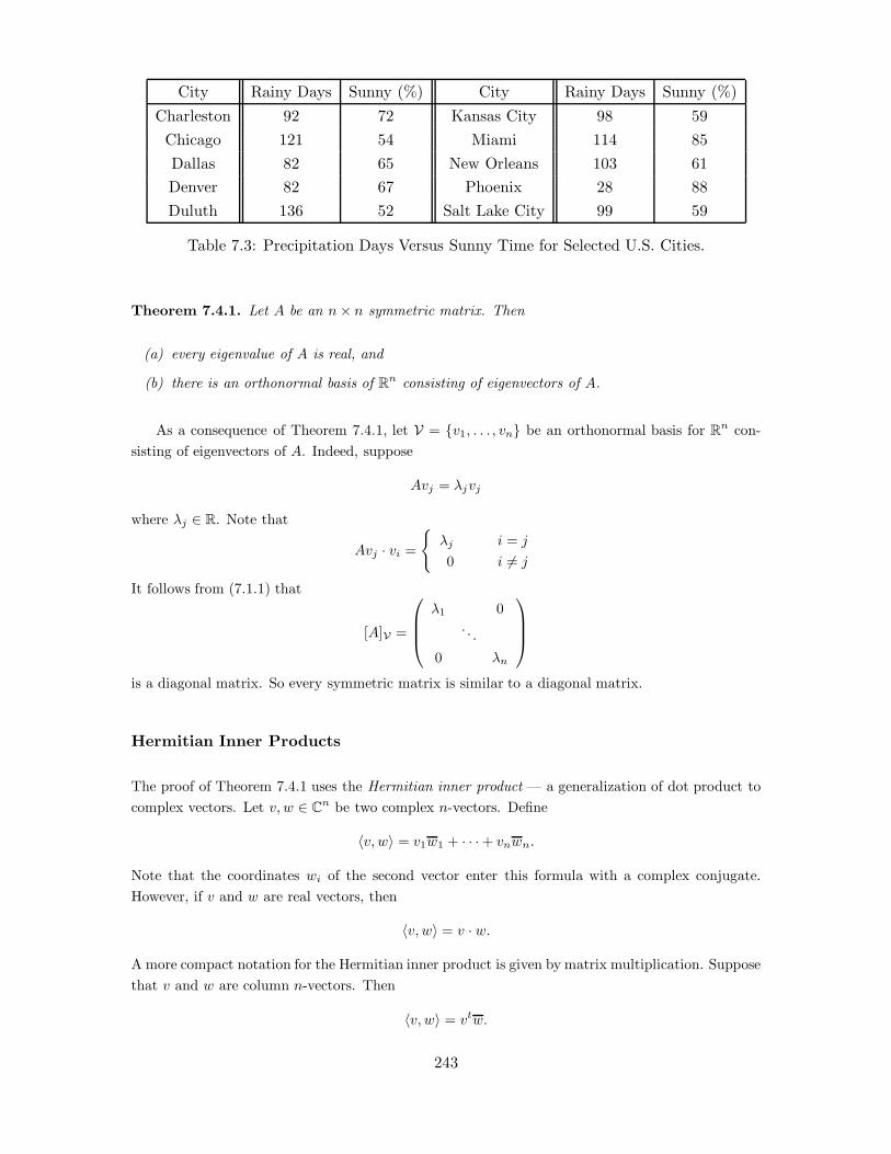
City Rainy Days Sunny (%) City Rainy Days Sunny (%)Charleston 92 72 Kansas City 98 59Chicago 121 54 Miami 114 85Dallas 82 65 New Orleans 103 61Denver 82 67 Phoenix 28 88Duluth 136 52 Salt Lake City 99 59

Table 7.3: Precipitation Days Versus Sunny Time for Selected U.S. Cities.

Theorem 7.4.1. Let A be an n" n symmetric matrix. Then

(a) every eigenvalue of A is real, and

(b) there is an orthonormal basis of Rn consisting of eigenvectors of A.

As a consequence of Theorem 7.4.1, let V = {v1, . . . , vn} be an orthonormal basis for Rn con-sisting of eigenvectors of A. Indeed, suppose

Avj = (jvj

where (j % R. Note that

Avj · vi =

9(j i = j

0 i #= j

It follows from (7.1.1) that

[A]V =

!

""#

(1 0.. .

0 (n

$

%%&

is a diagonal matrix. So every symmetric matrix is similar to a diagonal matrix.

Hermitian Inner Products

The proof of Theorem 7.4.1 uses the Hermitian inner product — a generalization of dot product tocomplex vectors. Let v, w % Cn be two complex n-vectors. Define

3v, w4 = v1w1 + · · ·+ vnwn.

Note that the coordinates wi of the second vector enter this formula with a complex conjugate.However, if v and w are real vectors, then

3v, w4 = v · w.

A more compact notation for the Hermitian inner product is given by matrix multiplication. Supposethat v and w are column n-vectors. Then

3v, w4 = vtw.

243

The properties of the Hermitian inner product are similar to those of dot product. We notethree. Let c % C be a complex scalar. Then

3v, v4 = ||v||2 ' 0

3cv, w4 = c3v, w4

3v, cw4 = c3v, w4

Note the complex conjugation of the complex scalar c in the previous formula.

Let C be a complex n " n matrix. Then the main observation concerning Hermitian innerproducts that we shall use is:

3Cv, w4 = 3v, Ctw4.

This fact is verified by calculating

3Cv, w4 = (Cv)tw = (vtCt)w = vt(Ctw) = vt(Ctw) = 3v, C

tw4.

So if A is a n" n real symmetric matrix, then

3Av, w4 = 3v, Aw4, (7.4.1)

since At = At = A.

Proof of Theorem 7.4.1(a): Let ( be an eigenvalue of A and let v be the associated eigenvector.Since Av = (v we can use (7.4.1) to compute

(3v, v4 = 3Av, v4 = 3v, Av4 = (3v, v4.

Since 3v, v4 = ||v||2 > 0, it follows that ( = ( and ( is real.

Proof of Theorem 7.4.1(b): Let A be a real symmetric n " n matrix. We want to show thatthere is an orthonormal basis of Rn consisting of eigenvectors of A. The proof proceeds inductivelyon n. The theorem is trivially valid for n = 1; so we assume that it is valid for n! 1.

Theorem 4.3.4 of Chapter 4 implies that A has an eigenvalue (1 and Theorem 7.4.1(a) statesthat this eigenvalue is real. Let v1 be a unit length eigenvector corresponding to the eigenvalue (1.Extend v1 to an orthonormal basis v1, w2, . . . , wn of Rn and let P = (v1|w2| · · · |wn) be the matrixwhose columns are the vectors in this orthonormal basis. Orthonormality and direct multiplicationimplies that

P tP = In. (7.4.2)

Therefore P is invertible; indeed P#1 = P t.

Next, letB = P#1AP.

By direct computation

Be1 = P#1APe1 = P#1Av1 = (1P#1v1 = (1e1.

It follows that that B has the form

B =

'(1 &0 C

(

244

where C is an (n ! 1) " (n ! 1) matrix. Since P#1 = P t, it follows that B is a symmetric matrix;to verify this point compute

Bt = (P tAP )t = P tAt(P t)t = P tAP = B.

It follows that

B =

'(1 00 C

(

where C is a symmetric matrix. By induction we can choose an orthonormal basis z2, . . . , zn in{0}"Rn#1 consisting of eigenvectors of C. It follows that e1, z2, . . . , zn is an orthonormal basis forRn consisting of eigenvectors of B.

Finally, let vj = P#1zj for j = 2, . . . , n. Since v1 = P#1e1, it follows that v1, v2, . . . , vn is a basisof Rn consisting of eigenvectors of A. We need only show that the vj form an orthonormal basis ofRn. This is done using (7.4.1). For notational convenience let z1 = e1 and compute

3vi, vj4 = 3P#1zi, P#1zj4 = 3P tzi, P

tzj4 = 3zi, PP tzj4 = 3zi, zj4,

since PP t = In. Thus the vectors vj form an orthonormal basis since the vectors zj form anorthonormal basis.

Hand Exercises

1. Let

A =

'a b

b d

(

be the general real 2" 2 symmetric matrix.

(a) Prove directly using the discriminant of the characteristic polynomial that A has real eigen-values.

(b) Show that A has equal eigenvalues only if A is a scalar multiple of I2.

2. Let

A =

'1 22 !2

(.

Find the eigenvalues and eigenvectors of A and verify that the eigenvectors are orthogonal.

Computer Exercises

In Exercises 3 – 5 compute the eigenvalues and the eigenvectors of the 2 " 2 matrix. Then loadthe matrix into the program map in MATLAB and iterate. That is, choose an initial vector v0 anduse map to compute v1 = Av0, v2 = Av1, . . . . How does the result of iteration compare with theeigenvectors and eigenvalues that you have found? Hint: You may find it convenient to use thefeature Rescale in the MAP Options. Then the norm of the vectors is rescaled to 1 after each use ofthe command Map and the vectors vj will not escape from the viewing screen.

245

3. A =

'1 33 1

(

4. B =

'11 99 11

(

5. C =

'0.005 !2.005!2.005 0.005

(

6. Perform the same computational experiment as described in Exercises 3 – 5 using the matrix

A =

'0 22 0

(and the program map. How do your results di!er from the results in those exercises

and why?

7.5 Orthogonal Matrices and QR Decompositions

In this section we describe an alternative approach to Gram-Schmidt orthonormalization for con-structing an orthonormal basis of a subspace W 1 Rn. This method is called the QR decompositionand is numerically superior to Gram-Schmidt. Indeed, the QR decomposition is the method usedby MATLAB to compute orthonormal bases. To discuss this decomposition we need to introduce anew type of matrices, the orthogonal matrices.

Orthogonal Matrices

Definition 7.5.1. An n " n matrix Q is orthogonal if its columns form an orthonormal basis ofRn.

The following lemma states elementary properties of orthogonal matrices:

Lemma 7.5.2. Let Q be an n" n matrix. Then

(a) Q is orthogonal if and only if QtQ = In;

(b) Q is orthogonal if and only if Q#1 = Qt;

(c) If Q1, Q2 are orthogonal matrices, then Q1Q2 is an orthogonal matrix.

Proof: (a) Let Q = (v1| · · · |vn). Since Q is orthogonal, the vj form an orthonormal basis. Bydirect computation note that QtQ = {(vi · vj)} = In, since the vj are orthonormal. Note that (b) issimply a restatement of (a).

(c) Now let Q1, Q2 be orthogonal. Then (a) implies

(Q1Q2)t(Q1Q2) = Qt2Q

t1Q1Q2 = Qt

2Q2 = In,

thus proving (c).

246

The previous lemma together with (7.4.2) in the proof of Theorem 7.4.1(b) lead to the followingresult:

Proposition 7.5.3. For each symmetric n" n matrix A, there exists an orthogonal matrix P suchthat P tAP is a diagonal matrix.

Reflections Across Hyperplanes: Householder Matrices

Useful examples of orthogonal matrices are reflections across hyperplanes. An n ! 1 dimensionalsubspace of Rn is called a hyperplane. Let V be a hyperplane and let u be a nonzero vector normalto V . Then a reflection across V is a linear map H : Rn * Rn such that

(a) Hv = v for all v % V .

(b) Hu = !u.

We claim that the matrix of a reflection across a hyperplane is orthogonal and there is a simpleformula for that matrix.

Definition 7.5.4. A Householder matrix is an n" n matrix of the form

H = In !2

utuuut (7.5.1)

where u % Rn is a nonzero vector. .

This definition makes sense since utu = ||u||2 is a number while the product uut is an n " n

matrix.

Lemma 7.5.5. Let u % Rn be a nonzero vector and let V be the hyperplane orthogonal to u. Thenthe Householder matrix H is a reflection across V and is orthogonal.

Proof: By definition every vector v % V satisfies utv = u · v = 0. Therefore,

Hv = v ! 2utu

uutv = v,

andHu = u! 2

utuuutu = u! 2u = !u.

Hence H is a reflection across the hyperplane V . It also follows that H2 = In since H2v = H(Hv) =Hv = v for all v % V and H2u = H(!u) = u. So H2 acts like the identity on a basis of Rn andH2 = In.

To show that H is orthogonal, we first calculate

Ht = Itn !

2utu

(uut)t = In !2

utuuut = H.

Therefore In = HH = HHt and Ht = H#1. Now apply Lemma 7.5.2(b).

247

QR Decompositions

The Gram-Schmidt process is not used in practice to find orthonormal bases as there are othertechniques available that are preferable for orthogonalization on a computer. One such procedurefor the construction of an orthonormal basis is based on QR decompositions using Householdertransformations. This method is the one implemented in MATLAB .

An n" k matrix R = {rij} is upper triangular if rij = 0 whenever i > j.

Definition 7.5.6. An n" k matrix A has a QR decomposition if

A = QR. (7.5.2)

where Q is an n" n orthogonal matrix and R is an n" k upper triangular matrix R.

QR decompositions can be used to find orthonormal bases as follows. Suppose that W ={w1, . . . , wk} is a basis for the subspace W 1 Rn. Then define the n" k matrix A which has the wj

as columns, that isA = (wt

1| · · · |wtk).

Suppose that A = QR is a QR decomposition. Since Q is orthogonal, the columns of Q areorthonormal. So write

Q = (vt1| · · · |vt

n).

On taking transposes we arrive at the equation At = RtQt:

!

""#

w1

...wk

$

%%& =

!

""""#

r11 0 · · · 0 · · · 0r12 r22 · · · 0 · · · 0...

... · · ·... · · ·

...r1k r2k · · · rkk · · · 0

$

%%%%&

!

""#

v1

...vn

$

%%& .

By equating rows in this matrix equation we arrive at the system

w1 = r11v1

w2 = r12v1 + r22v2

...wk = r1kv1 + r2kv2 + · · ·+ rkkvk.

(7.5.3)

It now follows that the W = span{v1, . . . , vk} and that {v1, . . . , vk} is an orthonormal basis for W .We have proved:

Proposition 7.5.7. Suppose that there exist an orthogonal n"n matrix Q and an upper triangularn" k matrix R such that the n" k matrix A has a QR decomposition

A = QR.

Then the first k columns v1, . . . , vk of the matrix Q form an orthonormal basis of the subspaceW = span{w1, . . . , wk}, where the wj are the columns of A. Moreover, rij = vi ·wj is the coordinateof wj in the orthonormal basis.

248

Conversely, we can also write down a QR decomposition for a matrix A, if we have computed anorthonormal basis for the columns of A. Indeed, using the Gram-Schmidt process, Theorem 7.2.3,we have shown that QR decompositions always exist. In the remainder of this section we discuss adi"erent way for finding QR decompositions using Householder matrices.

Construction of a QR Decomposition Using Householder Matrices

The QR decomposition by Householder transformations is based on the following observation :

Proposition 7.5.8. Let z = (z1, . . . , zn) % Rn be nonzero and let

r =)

z2j + · · ·+ z2

n.

Define u = (u1, . . . , un) % Rn by!

""""""""""""#

u1

...uj#1

uj

uj+1

...un

$

%%%%%%%%%%%%&

=

!

""""""""""""#

0...0

zj ! r

zj+1

...zn

$

%%%%%%%%%%%%&

.

Then2utz = utu

and

Hz =

!

""""""""""""#

z1

...zj#1

r

0...0

$

%%%%%%%%%%%%&

(7.5.4)

holds for the Householder matrix H = In ! 2utuuut.

Proof: Begin by computing

utz = ujzj + z2j+1 + · · ·+ z2

n

= z2j ! rzj + z2

j+1 + · · ·+ z2n

= !rzj + r2.

Next, compute

utu = (zj ! r)(zj ! r) + z2j+1 + · · ·+ z2

n

= z2j ! 2rzj + r2 + z2

j+1 + · · ·+ z2n

= 2(!rzj + r2).

249

Hence 2utz = utu, as claimed.

Note that z ! u is the vector on the right hand side of (7.5.4). So, compute

Hz =*

In !2

utuuut

+z = z ! 2utz

utuu = z ! u

to see that (7.5.4) is valid.

An inspection of the proof of Proposition 7.5.8 shows that we could have chosen

uj = zj + r

instead of uj = zj ! r. Therefore, the choice of H is not unique.

Proposition 7.5.8 allows us to determine inductively a QR decomposition of the matrix

A = (w01| · · · |w0

k),

where each w0j % Rn. So, A is an n" k matrix and k ( n.

First, set z = w01 and use Proposition 7.5.8 to construct the Householder matrix H1 such that

H1w01 =

!

""""#

r11

0...0

$

%%%%&, r1.

Then the matrix A1 = H1A can be written as

A1 = (r1|w12| · · · |w1

k),

where w1j = H1w0

j for j = 2, . . . , k.

Second, set z = w12 in Proposition 7.5.8 and construct the Householder matrix H2 such that

H2w12 =

!

""""""#

r12

r22

0...0

$

%%%%%%&, r2.

Then the matrix A2 = H2A1 = H2H1A can be written as

A2 = (r1|r2|w23| · · · |w2

k)

where w2j = H2w1

j for j = 3, . . . , k. Observe that the 1st column r1 is not a"ected by the matrixmultiplication, since H2 leaves the first component of a vector unchanged.

Proceeding inductively, in the ith step, set z = wi#1i and use Proposition 7.5.8 to construct the

250

Householder matrix Hi such that:

Hiwi#1i =

!

""""""""""#

r1i

...rii

0...0

$

%%%%%%%%%%&

, ri

and the matrix Ai = HiAi#1 = Hi · · ·H1A can be written as

Ai = (r1| · · · |ri|wii+1| · · · |wi

k),

where w2i = Hiw

i#1j for j = i + 1, . . . , k.

After k steps we arrive atHk · · ·H1A = R,

where R = (r1| · · · |rk) is an upper triangular n " k matrix. Since the Householder matricesH1, . . . , Hk are orthogonal, it follows from Lemma 7.5.2(c) that the Qt = Hk · · ·H1 is orthogonal.Thus, A = QR is a QR decomposition of A.

Orthonormalization with MATLAB

Given a set w1, . . . , wk of linearly independent vectors in Rn the MATLAB command qr allowsus to compute an orthonormal basis of the spanning set of these vectors. As mentioned earlier,the underlying technique MATLAB uses for the computation of the QR decomposition is based onHouseholder transformations.

The syntax of the QR decomposition in MATLAB is quite simple. For example, let w1 =(1, 0,!1, 0), w2 = (2,!1, 0, 1) and w3 = (0, 0,!2, 1) be the three vectors in (7.2.11). In Section 5.5we computed an orthonormal basis for the subspace of R4 spanned by w1, w2, w3. Here we use theMATLAB command qr to find an orthonormal basis for this subspace. Let A be the matrix havingthe vectors wt

1, wt2 and wt

3 as columns. So, A is:

A = [1 2 0; 0 -1 0; -1 0 -2; 0 1 1]

The command

[Q R] = qr(A,0)

leads to the answer

Q =

-0.7071 0.5000 -0.4523

251

0 -0.5000 -0.1508

0.7071 0.5000 -0.4523

0 0.5000 0.7538

R =

-1.4142 -1.4142 -1.4142

0 2.0000 -0.5000

0 0 1.6583

A comparison with (7.2.12) shows that the columns of the matrix Q are the elements in the or-thonormal basis. The only di"erence is that the sign of the first vector is opposite. However, this isnot surprising since we know that there is some freedom in the choice of Householder matrices, asremarked after Proposition 7.5.8.

In addition, the command qr produces the matrix R whose entries rij are the coordinates of thevectors wj in the new orthonormal basis as in (7.5.3). For instance, the second column of R tells usthat

w2 = r12v1 + r22v2 + r32v3 = !1.4142v1 + 2.0000v2.

Hand Exercises

In Exercises 1 – 5 decide whether or not the given matrix is orthogonal.

1.

'2 00 1

(.

2.

!

"#0 1 00 0 11 0 0

$

%&.

3.

!

"#0 !1 00 0 1!1 0 0

$

%&.

4.

'cos(1) ! sin(1)sin(1) cos(1)

(.

5.

'1 0 40 1 0

(.

6. Let Q be an orthogonal n" n matrix. Show that Q preserves the length of vectors, that is

5Qv5 = 5v5 for all v % Rn.

In Exercises 7 – 10, compute the Householder matrix H corresponding to the given vector u.

252

7. u =

'11

(.

8. u =

'0!2

(.

9. u =

!

"#!1

15

$

%&.

10. u =

!

"""#

104!2

$

%%%&.

11. Find the matrix that reflects the plane across the line generated by the vector (1, 2).

12. Prove that the rows of an n" n orthogonal matrix form an orthonormal basis for Rn.

Computer Exercises

In Exercises 13 – 16, use the MATLAB command qr to compute an orthonormal basis for eachof the subspaces spanned by the given set of vectors.

13. w1 = (1,!1), w2 = (1, 2).

14. w1 = (1,!2, 3), w2 = (0, 1, 1).

15. w1 = (1,!2, 3), w2 = (0, 1, 1), w3 = (2, 2, 0).

16. v1 = (1, 0,!2, 0,!1), v2 = (2,!1, 4, 2, 0), v3 = (0, 3, 5, 1,!1).

17. Find the 4" 4 Householder matrices H1 and H2 corresponding to the vectors

u1 = (1.04, 2, 0.76,!0.32)u2 = (1.4,!1.3, 0.6, 1.2).

Compute H = H1H2 and verify that H is an orthogonal matrix.

253

Chapter 8

Matrix Normal Forms

In this chapter we generalize to n!n matrices the theory of matrix normal forms presentedin Chapter ?? for 2 ! 2 matrices. In this theory we ask: What is the simplest form thata matrix can have up to similarity . After first presenting several preliminary results, thetheory culminates in the Jordan normal form theorem, Theorem 8.4.2.

The first of the matrix normal form results — every matrix with n distinct real eigen-values can be diagonalized — is presented in Section 8.1. The basic idea is that when amatrix has n distinct real eigenvalues, then it has n linearly independent eigenvectors. InSection 8.2 we discuss matrix normal forms when the matrix has n distinct eigenvaluessome of which are complex. When an n ! n matrix has fewer than n linearly independenteigenvectors, it must have multiple eigenvalues and generalized eigenvectors. This topic isdiscussed in Section 8.3. The Jordan normal form theorem is introduced in Section 8.4 anddescribes similarity of matrices when the matrix has fewer than n independent eigenvectors.The proof is given in Appendix 8.6.

We introduced Markov matrices in Section 4.5. One of the theorems discussed therehas a proof that relies on the Jordan normal form theorem, and we prove this theorem inAppendix 8.5.

8.1 Real Diagonalizable Matrices

An n ! n matrix is real diagonalizable if it is similar to a diagonal matrix. More precisely,an n ! n matrix A is real diagonalizable if there exists an invertible n ! n matrix S suchthat

D = S#1AS

254

is a diagonal matrix. In this section we investigate when a matrix is diagonalizable. In thisdiscussion we assume that all matrices have real entries.

We begin with the observation that not all matrices are real diagonalizable. We sawin Example 4.3.2 that the diagonal entries of the diagonal matrix D are the eigenvalues ofD. Theorem 4.3.8 states that similar matrices have the same eigenvalues. Thus if a matrixis real diagonalizable, then it must have real eigenvalues. It follows, for example, that the2 ! 2 matrix '

0 "11 0

(

is not real diagonalizable, since its eigenvalues are ±i.

However, even if a matrix A has real eigenvalues, it need not be diagonalizable. Forexample, the only matrix similar to the identity matrix In is the identity matrix itself. Toverify this point, calculate

S#1InS = S#1S = In.

Suppose that A is a matrix all of whose eigenvalues are equal to 1. If A is similar to adiagonal matrix D, then D must have all of its eigenvalues equal to 1. Since the identitymatrix is the only diagonal matrix with all eigenvalues equal to 1, D = In. So, if A issimilar to a diagonal matrix, it must itself be the identity matrix. Consider, however, the2 ! 2 matrix

A =

'1 10 1

(

.

Since A is triangular, it follows that both eigenvalues of A are equal to 1. Since A is notthe identity matrix, it cannot be diagonalizable. More generally, if N is a nonzero strictlyupper triangular n ! n matrix, then the matrix In + N is not diagonalizable.

These examples show that complex eigenvalues are always obstructions to real diag-onalization and multiple real eigenvalues are sometimes obstructions to diagonalization.Indeed,

Theorem 8.1.1. Let A be an n!n matrix with n distinct real eigenvalues. Then A is realdiagonalizable.

There are two ideas in the proof of Theorem 8.1.1, and they are summarized in thefollowing lemmas.

Lemma 8.1.2. Let &1, . . . ,&k be distinct real eigenvalues for an n!n matrix A. Let vj beeigenvectors associated with the eigenvalue &j. Then {v1, . . . , vk} is a linearly independentset.

255

Proof: We prove the lemma by using induction on k. When k = 1 the proof is simple,since v1 %= 0. So we can assume that {v1, . . . , vk#1} is a linearly independent set.

Let "1, . . . ,"k be scalars such that

"1v1 + · · ·+ "kvk = 0. (8.1.1)

We must show that all "j = 0.

Begin by multiplying both sides of (8.1.1) by A, to obtain:

0 = A("1v1 + · · ·+ "kvk)

= "1Av1 + · · ·+ "kAvk (8.1.2)

= "1&1v1 + · · ·+ "k&kvk .

Now subtract &k times (8.1.1) from (8.1.2), to obtain:

"1(&1 " &k)v1 + · · ·+ "k#1(&k#1 " &k)vk#1 = 0.

Since {v1, . . . , vk#1} is a linearly independent set, it follows that

"j(&j " &k) = 0,

for j = 1, . . . , k " 1. Since all of the eigenvalues are distinct, &j " &k %= 0 and "j = 0 forj = 1, . . . , k " 1. Substituting this information into (8.1.1) yields "kvk = 0. Since vk %= 0,"k is also equal to zero.

Lemma 8.1.3. Let A be an n ! n matrix. Then A is real diagonalizable if and only if A

has n real linearly independent eigenvectors.

Proof: Suppose that A has n linearly independent eigenvectors v1, . . . , vn. Let &1, . . . ,&n

be the corresponding eigenvalues of A; that is, Avj = &jvj . Let S = (v1| · · · |vn) be the n!n

matrix whose columns are the eigenvectors vj . We claim that D = S#1AS is a diagonalmatrix. Compute

D = S#1AS = S#1A(v1| · · · |vn) = S#1(Av1| · · · |Avn) = S#1(&1v1| · · · |&nvn).

It follows thatD = (&1S

#1v1| · · · |&nS#1vn).

Note thatS#1vj = ej ,

sinceSej = vj .

256

Therefore,D = (&1e1| · · · |&nen)

is a diagonal matrix.

Conversely, suppose that A is a real diagonalizable matrix. Then there exists an invert-ible matrix S such that D = S#1AS is diagonal. Let vj = Sej . We claim that {v1, . . . , vn}is a linearly independent set of eigenvectors of A.

Since D is diagonal, Dej = &jej for some real number &j . It follows that

Avj = SDS#1vj = SDS#1Sej = SDej = &jSej = &jvj .

So vj is an eigenvector of A. Since the matrix S is invertible, its columns are linearlyindependent. Since the columns of S are vj , the set {v1, . . . , vn} is a linearly independentset of eigenvectors of A, as claimed.

Proof of Theorem 8.1.1: Let &1, . . . ,&n be the distinct eigenvalues of A and let v1, . . . , vn

be the corresponding eigenvectors. Lemma 8.1.2 implies that {v1, . . . , vn} is a linearlyindependent set in Rn and therefore a basis. Lemma 8.1.3 implies that A is diagonalizable.

Diagonalization Using MATLAB

Let

A =

!

"#"6 12 4

8 "21 "8"29 72 27

$

%& .

We use MATLAB to answer the questions: Is A real diagonalizable and, if it is, can we findthe matrix S such that S#1AS is diagonal? We can find the eigenvalues of A by typingeig(A). MATLAB’s response is:

ans =

-2.0000

-1.0000

3.0000

Since the eigenvalues of A are real and distinct, Theorem 8.1.1 states that A can be diago-nalized. That is, there is a matrix S such that

S#1AS =

!

"#"1 0 0

0 "2 00 0 3

$

%&

257

The proof of Lemma 8.1.3 tells us how to find the matrix S. We need to find the eigenvectorsv1, v2, v3 associated with the eigenvalues "1,"2, 3, respectively. Then the matrix (v1|v2|v3)whose columns are the eigenvectors is the matrix S. To verify this construction we first findthe eigenvectors of A by typing

v1 = null(A+eye(3));

v2 = null(A+2*eye(3));

v3 = null(A-3*eye(3));

Now type S = [v1 v2 v3] to obtain

S =

0.8729 0.7071 0

0.4364 0.0000 0.3162

-0.2182 0.7071 -0.9487

Finally, check that S#1AS is the desired diagonal matrix by typing inv(S)*A*S to obtain

ans =

-1.0000 0.0000 0

0.0000 -2.0000 -0.0000

0.0000 0 3.0000

It is cumbersome to use the null command to find eigenvectors and MATLAB has beenpreprogrammed to do these computations automatically. We can use the eig command tofind the eigenvectors and eigenvalues of a matrix A, as follows. Type

[S,D] = eig(A)

and MATLAB responds with

S =

-0.7071 0.8729 -0.0000

-0.0000 0.4364 -0.3162

-0.7071 -0.2182 0.9487

D =

-2.0000 0 0

0 -1.0000 0

0 0 3.0000

258

The matrix S is the transition matrix whose columns are the eigenvectors of A and thematrix D is a diagonal matrix whose jth diagonal entry is the eigenvalue of A correspondingto the eigenvector in the jth column of S.

Hand Exercises

1. Let A =

'0 33 0

(.

(a) Find the eigenvalues and eigenvectors of A.

(b) Find an invertible matrix S such that S#1AS is a diagonal matrix D. What is D?

2. The eigenvalues of

A =

!

"#!1 2 !1

3 0 1!3 !2 !3

$

%&

are 2,!2,!4. Find the eigenvectors of A for each of these eigenvalues and find a 3 " 3 invertiblematrix S so that S#1AS is diagonal.

3. Let

A =

!

"#!1 4 !2

0 3 !20 4 !3

$

%& .

Find the eigenvalues and eigenvectors of A, and find an invertible matrix S so that S#1AS isdiagonal.

4. Let A and B be similar n" n matrices.

(a) Show that if A is invertible, then B is invertible.

(b) Show that A + A#1 is similar to B + B#1.

5. Let A and B be n " n matrices. Suppose that A is real diagonalizable and that B is similar toA. Show that B is real diagonalizable.

6. Let A be an n " n real diagonalizable matrix. Show that A + $In is also real diagonalizable.

7. Let A be an n"n matrix with a real eigenvalue ( and associated eigenvector v. Assume that allother eigenvalues of A are di"erent from (. Let B be an n" n matrix that commutes with A; thatis, AB = BA. Show that v is also an eigenvector for B.

8. Let A be an n " n matrix with distinct real eigenvalues and let B be an n " n matrix thatcommutes with A. Using the result of Exercise 7, show that there is a matrix S that simultaneouslydiagonalizes A and B; that is, S#1AS and S#1BS are both diagonal matrices.

9. Let A be an n " n matrix all of whose eigenvalues equal ±1. Show that if A is diagonalizable,the A2 = In.

259

10. Let A be an n"n matrix all of whose eigenvalues equal 0 and 1. Show that if A is diagonalizable,the A2 = A.

Computer Exercises

11. Consider the 4" 4 matrix

C =

!

"""#

12 48 68 88!19 !54 !57 !68

22 52 66 96!11 !26 !41 !64

$

%%%&.

Use MATLAB to show that the eigenvalues of C are real and distinct. Find a matrix S so thatS#1CS is diagonal.

In Exercises 12 – 13 use MATLAB to decide whether or not the given matrix is real diagonalizable.

12.

A =

!

"""#

!2.2 4.1 !1.5 !0.2!3.4 4.8 !1.0 0.2!1.0 0.4 1.9 0.2!14.5 17.8 !6.7 0.6

$

%%%&.

13.

B =

!

""""""#

1.9 2.2 1.5 !1.6 !2.80.8 2.6 1.5 !1.8 !2.02.6 2.8 1.6 !2.1 !3.84.8 3.6 1.5 !3.1 !5.2!2.1 1.2 1.7 !0.2 0.0

$

%%%%%%&.

8.2 Simple Complex Eigenvalues

Theorem 8.1.1 states that a matrix A with real unequal eigenvalues may be diagonalized. It followsthat in an appropriately chosen basis (the basis of eigenvectors), matrix multiplication by A actsas multiplication by these real eigenvalues. Moreover, geometrically, multiplication by A stretchesor contracts vectors in eigendirections (depending on whether the eigenvalue is greater than or lessthan 1 in absolute value).

The purpose of this section is to show that a similar kind of diagonalization is possible whenthe matrix has distinct complex eigenvalues. See Theorem 8.2.1 and Theorem 8.2.2. We showthat multiplication by a matrix with complex eigenvalues corresponds to multiplication by complexnumbers. We also show that multiplication by complex eigenvalues correspond geometrically torotations as well as expansions and contractions.

260

The Geometry of Complex Eigenvalues: Rotations and Dilatations

Real 2" 2 matrices are the smallest real matrices where complex eigenvalues can possibly occur. InChapter ??, Theorem ??(b) we discussed the classification of such matrices up to similarity. Recallthat if the eigenvalues of a 2" 2 matrix A are * ± i, , then A is similar to the matrix

'* !,, *

(. (8.2.1)

Moreover, the basis in which A has the form (8.2.1) is found as follows. Let v = w1 + iw2 be theeigenvector of A corresponding to the eigenvalue * ! i, . Then {w1, w2} is the desired basis.

Geometrically, multiplication of vectors in R2 by (8.2.1) is the same as a rotation followed bya dilatation. More specifically, let r =

$*2 + ,2. So the point (*, , ) lies on the circle of radius r

about the origin, and there is an angle ! such that (*, , ) = (r cos !, r sin !). Now we can rewrite(8.2.1) as '

* !,, *

(= r

'cos ! ! sin !sin ! cos !

(= rR#,

where R# is rotation counterclockwise through angle !. From this discussion we see that geometricallycomplex eigenvalues are associated with rotations followed either by stretching (r > 1) or contracting(r < 1).

As an example, consider the matrix

A =

'2 1!2 0

(. (8.2.2)

The characteristic polynomial of A is pA(() = (2 ! 2( + 2. Thus the eigenvalues of A are 1 ± i,and * = 1 and , = 1 for this example. An eigenvector associated to the eigenvalue 1 ! i isv = (1,!1! i)t = (1,!1)t + i(0,!1)t. Therefore,

B = S#1AS =

'1 !11 1

(where S =

'1 0!1 !1

(,

as can be checked by direct calculation. Moreover, we can rewrite

B =$

2

' $2

2 !$

22$

22

$2

2

(=$

2R!4.

So, in an appropriately chosen coordinate system, multiplication by A rotates vectors counterclock-wise by 45" and then expands the result by a factor of

$2. See Exercise 3.

The Algebra of Complex Eigenvalues: Complex Multiplication

We have shown that the normal form (8.2.1) can be interpreted geometrically as a rotation followedby a dilatation. There is a second algebraic interpretation of (8.2.1), and this interpretation is basedon multiplication by complex numbers.

261

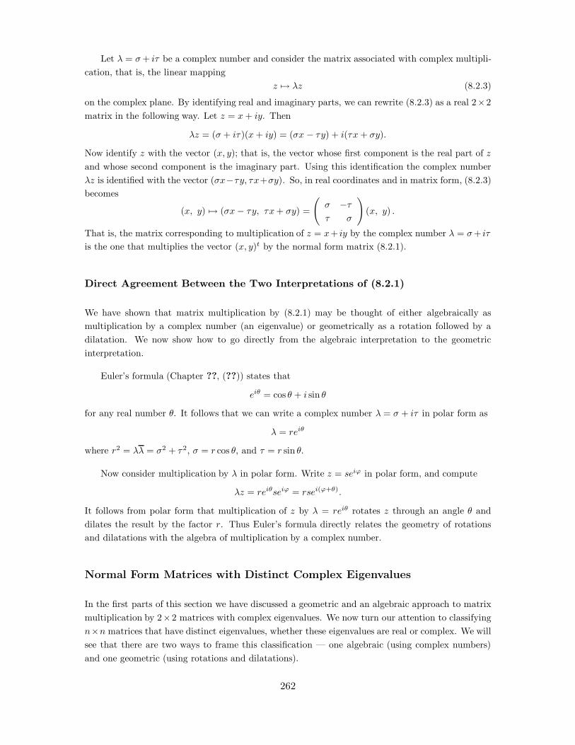
Let ( = *+ i, be a complex number and consider the matrix associated with complex multipli-cation, that is, the linear mapping

z )* (z (8.2.3)

on the complex plane. By identifying real and imaginary parts, we can rewrite (8.2.3) as a real 2"2matrix in the following way. Let z = x + iy. Then

(z = (* + i, )(x + iy) = (*x ! ,y) + i(,x + *y).

Now identify z with the vector (x, y); that is, the vector whose first component is the real part of z

and whose second component is the imaginary part. Using this identification the complex number(z is identified with the vector (*x!,y, ,x+*y). So, in real coordinates and in matrix form, (8.2.3)becomes

(x, y) )* (*x! ,y, ,x + *y) =

'* !,, *

((x, y) .

That is, the matrix corresponding to multiplication of z = x+ iy by the complex number ( = *+ i,

is the one that multiplies the vector (x, y)t by the normal form matrix (8.2.1).

Direct Agreement Between the Two Interpretations of (8.2.1)

We have shown that matrix multiplication by (8.2.1) may be thought of either algebraically asmultiplication by a complex number (an eigenvalue) or geometrically as a rotation followed by adilatation. We now show how to go directly from the algebraic interpretation to the geometricinterpretation.

Euler’s formula (Chapter ??, (??)) states that

ei# = cos ! + i sin !

for any real number !. It follows that we can write a complex number ( = * + i, in polar form as

( = rei#

where r2 = (( = *2 + ,2, * = r cos !, and , = r sin !.

Now consider multiplication by ( in polar form. Write z = sei$ in polar form, and compute

(z = rei#sei$ = rsei($+#).

It follows from polar form that multiplication of z by ( = rei# rotates z through an angle ! anddilates the result by the factor r. Thus Euler’s formula directly relates the geometry of rotationsand dilatations with the algebra of multiplication by a complex number.

Normal Form Matrices with Distinct Complex Eigenvalues

In the first parts of this section we have discussed a geometric and an algebraic approach to matrixmultiplication by 2"2 matrices with complex eigenvalues. We now turn our attention to classifyingn"n matrices that have distinct eigenvalues, whether these eigenvalues are real or complex. We willsee that there are two ways to frame this classification — one algebraic (using complex numbers)and one geometric (using rotations and dilatations).

262

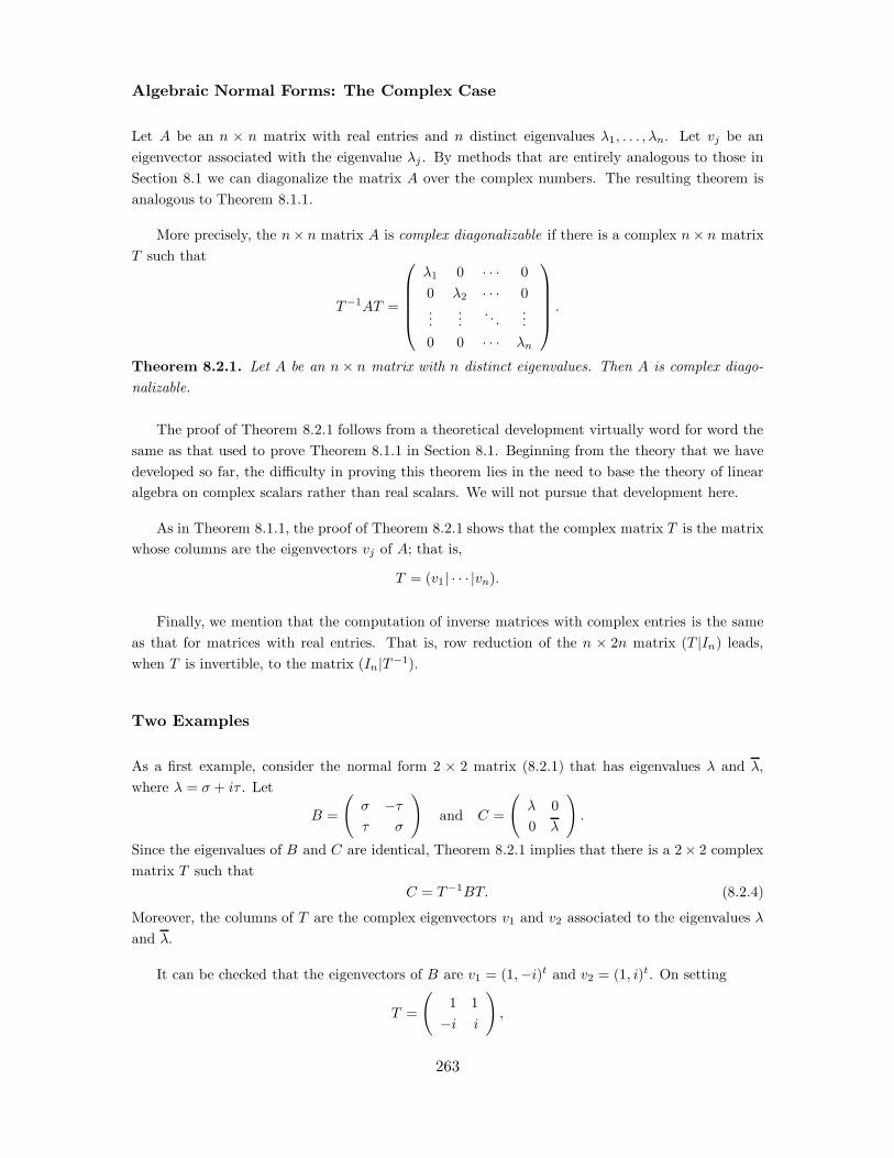
Algebraic Normal Forms: The Complex Case

Let A be an n " n matrix with real entries and n distinct eigenvalues (1, . . . ,(n. Let vj be aneigenvector associated with the eigenvalue (j . By methods that are entirely analogous to those inSection 8.1 we can diagonalize the matrix A over the complex numbers. The resulting theorem isanalogous to Theorem 8.1.1.

More precisely, the n" n matrix A is complex diagonalizable if there is a complex n" n matrixT such that

T#1AT =

!

""""#

(1 0 · · · 00 (2 · · · 0...

.... . .

...0 0 · · · (n

$

%%%%&.

Theorem 8.2.1. Let A be an n" n matrix with n distinct eigenvalues. Then A is complex diago-nalizable.

The proof of Theorem 8.2.1 follows from a theoretical development virtually word for word thesame as that used to prove Theorem 8.1.1 in Section 8.1. Beginning from the theory that we havedeveloped so far, the di!culty in proving this theorem lies in the need to base the theory of linearalgebra on complex scalars rather than real scalars. We will not pursue that development here.

As in Theorem 8.1.1, the proof of Theorem 8.2.1 shows that the complex matrix T is the matrixwhose columns are the eigenvectors vj of A; that is,

T = (v1| · · · |vn).

Finally, we mention that the computation of inverse matrices with complex entries is the sameas that for matrices with real entries. That is, row reduction of the n " 2n matrix (T |In) leads,when T is invertible, to the matrix (In|T#1).

Two Examples

As a first example, consider the normal form 2 " 2 matrix (8.2.1) that has eigenvalues ( and (,where ( = * + i, . Let

B =

'* !,, *

(and C =

'( 00 (

(.

Since the eigenvalues of B and C are identical, Theorem 8.2.1 implies that there is a 2" 2 complexmatrix T such that

C = T#1BT. (8.2.4)

Moreover, the columns of T are the complex eigenvectors v1 and v2 associated to the eigenvalues (and (.

It can be checked that the eigenvectors of B are v1 = (1,!i)t and v2 = (1, i)t. On setting

T =

'1 1!i i

(,

263

it is a straightforward calculation to verify that C = T#1BT .

As a second example, consider the matrix

A =

!

"#4 2 12 !3 11 !1 !3

$

%& .

Using MATLAB we find the eigenvalues of A by typing eig(A). They are:

ans =

4.6432

-3.3216 + 0.9014i

-3.3216 - 0.9014i

We can diagonalize (over the complex numbers) using MATLAB — indeed MATLAB is programmedto do these calculations over the complex numbers. Type [T,D] = eig(A) and obtain

T =

0.9604 -0.1299 + 0.1587i -0.1299 - 0.1587i

0.2632 0.0147 - 0.5809i 0.0147 + 0.5809i

0.0912 0.7788 - 0.1173i 0.7788 + 0.1173i

D =

4.6432 0 0

0 -3.3216 + 0.9014i 0

0 0 -3.3216 - 0.9014i

This calculation can be checked by typing inv(T)*A*T to see that the diagonal matrix D appears.One can also check that the columns of T are eigenvectors of A.

Note that the development here does not depend on the matrix A having real entries. Indeed,this diagonalization can be completed using n" n matrices with complex entries — and MATLABcan handle such calculations.

Geometric Normal Forms: Block Diagonalization

There is a second normal form theorem based on the geometry of rotations and dilatations for realn " n matrices A. In this normal form we determine all matrices A that have distinct eigenvalues— up to similarity by real n " n matrices S. The normal form results in matrices that are blockdiagonal with either 1" 1 blocks or 2" 2 blocks of the form (8.2.1) on the diagonal.

264

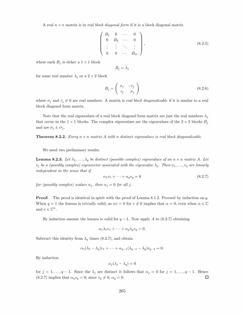
A real n " n matrix is in real block diagonal form if it is a block diagonal matrix!

""""#

B1 0 · · · 00 B2 · · · 0...

.... . .

...0 0 · · · Bm

$

%%%%&, (8.2.5)

where each Bj is either a 1" 1 blockBj = (j

for some real number (j or a 2" 2 block

Bj =

'*j !,j,j *j

((8.2.6)

where *j and ,j #= 0 are real numbers. A matrix is real block diagonalizable if it is similar to a realblock diagonal form matrix.

Note that the real eigenvalues of a real block diagonal form matrix are just the real numbers (j

that occur in the 1 " 1 blocks. The complex eigenvalues are the eigenvalues of the 2" 2 blocks Bj

and are *j ± i,j .

Theorem 8.2.2. Every n" n matrix A with n distinct eigenvalues is real block diagonalizable.

We need two preliminary results.

Lemma 8.2.3. Let (1, . . . ,(q be distinct (possible complex) eigenvalues of an n" n matrix A. Letvj be a (possibly complex) eigenvector associated with the eigenvalue (j. Then v1, . . . , vq are linearlyindependent in the sense that if

$1v1 + · · ·+ $qvq = 0 (8.2.7)

for (possibly complex) scalars $j, then $j = 0 for all j.

Proof: The proof is identical in spirit with the proof of Lemma 8.1.2. Proceed by induction on q.When q = 1 the lemma is trivially valid, as $v = 0 for v #= 0 implies that $ = 0, even when $ % Cand v % Cn.

By induction assume the lemma is valid for q ! 1. Now apply A to (8.2.7) obtaining

$1(1v1 + · · ·+ $q(qvq = 0.

Subtract this identity from (q times (8.2.7), and obtain

$1((1 ! (q)v1 + · · ·+ $q#1((q#1 ! (q)vq#1 = 0.

By induction$j((j ! (q) = 0

for j = 1, . . . , q ! 1. Since the (j are distinct it follows that $j = 0 for j = 1, . . . , q ! 1. Hence(8.2.7) implies that $qvq = 0; since vq #= 0, $q = 0.

265

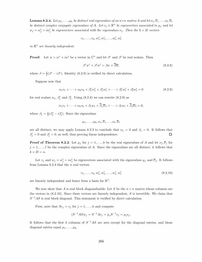
Lemma 8.2.4. Let µ1, . . . , µk be distinct real eigenvalues of an n"n matrix A and let .1, .1 . . . , .!, .!be distinct complex conjugate eigenvalues of A. Let vj % Rn be eigenvectors associated to µj and letwj = wr

j + iwij be eigenvectors associated with the eigenvalues .j. Then the k + 2# vectors

v1, . . . , vk, wr1, w

i1, . . . , w

r! , w

i!

in Rn are linearly independent.

Proof: Let w = wr + iwi be a vector in Cn and let %r and %i be real scalars. Then

%rwr + %iwi = %w + %w, (8.2.8)

where % = 12 (%r ! i%i). Identity (8.2.8) is verified by direct calculation.

Suppose now that

$1v1 + · · ·+ $kvk + %r1wr

1 + %i1w

i1 + · · ·+ %r

!wr! + %i

!wi! = 0 (8.2.9)

for real scalars $j, %rj and %i

j . Using (8.2.8) we can rewrite (8.2.9) as

$1v1 + · · ·+ $kvk + %1w1 + %1w1 + · · ·+ %!w! + %!w! = 0,

where %j = 12 (%r

j ! i%ij). Since the eigenvalues

µ1, . . . , µk, .1, .1 . . . , .!, .!

are all distinct, we may apply Lemma 8.2.3 to conclude that $j = 0 and %j = 0. It follows that%r

j = 0 and %ij = 0, as well, thus proving linear independence. .

Proof of Theorem 8.2.2: Let µj for j = 1, . . . , k be the real eigenvalues of A and let .j, .j forj = 1, . . . , # be the complex eigenvalues of A. Since the eigenvalues are all distinct, it follows thatk + 2# = n.

Let vj and wj = wrj + iwi

j be eigenvectors associated with the eigenvalues µj and .j. It followsfrom Lemma 8.2.4 that the n real vectors

v1, . . . , vk, wr1, w

i1, . . . , w

r! , w

i! (8.2.10)

are linearly independent and hence form a basis for Rn.

We now show that A is real block diagonalizable. Let S be the n" n matrix whose columns arethe vectors in (8.2.10). Since these vectors are linearly independent, S is invertible. We claim thatS#1AS is real block diagonal. This statement is verified by direct calculation.

First, note that Sej = vj for j = 1, . . . , k and compute

(S#1AS)ej = S#1Avj = µjS#1vj = µjej .

It follows that the first k columns of S#1AS are zero except for the diagonal entries, and thosediagonal entries equal µ1, . . . , µk.

266

Second, note that Sek+1 = wr1 and Sek+2 = wi

1. Write the complex eigenvalues as

.j = *j + i,j .

Since Aw1 = .1w1, it follows that

Awr1 + iAwi

1 = (*1 ! i,1)(wr1 + iwi

1)

= (*1wr1 + ,1wi

1) + i(!,1wr1 + *1w

i1).

Equating real and imaginary parts leads to

Awr1 = *1wr

1 + ,1wi1

Awi1 = !,1wr

1 + *1wi1.

(8.2.11)

Using (8.2.11), compute

(S#1AS)ek+1 = S#1Awr1 = S#1(*1w

r1 + ,1wi

1) = *1ek+1 + ,1ek+2.

Similarly,(S#1AS)ek+2 = S#1Awi

1 = S#1(!,1wr1 + *1w

i1) = !,1ek+1 + *1ek+2.

Thus, the kth and (k+1)st columns of S#1AS have the desired diagonal block in the kth and (k+1)st

rows, and have all other entries equal to zero.

The same calculation is valid for the complex eigenvalues .2, . . . , .!. Thus, S#1AS is real blockdiagonal, as claimed.

MATLAB Calculations of Real Block Diagonal Form

Let C be the 4" 4 matrix

C =

!

"""#

1 0 2 32 1 4 6!1 !5 1 3

1 4 7 10

$

%%%&.

Using MATLAB enter C by typing e13 2 14 and find the eigenvalues of C by typing eig(C) toobtain

ans =

0.5855 + 0.8861i

0.5855 - 0.8861i

-0.6399

12.4690

We see that C has two real and two complex conjugate eigenvalues. To find the complex eigenvectorsassociated with these eigenvalues, type

[T,D] = eig(C)

267

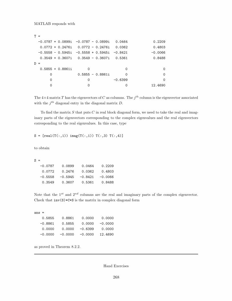
MATLAB responds with

T =

-0.0787 + 0.0899i -0.0787 - 0.0899i 0.0464 0.2209

0.0772 + 0.2476i 0.0772 - 0.2476i 0.0362 0.4803

-0.5558 - 0.5945i -0.5558 + 0.5945i -0.8421 -0.0066

0.3549 + 0.3607i 0.3549 - 0.3607i 0.5361 0.8488

D =

0.5855 + 0.8861i 0 0 0

0 0.5855 - 0.8861i 0 0

0 0 -0.6399 0

0 0 0 12.4690

The 4"4 matrix T has the eigenvectors of C as columns. The jth column is the eigenvector associatedwith the jth diagonal entry in the diagonal matrix D.

To find the matrix S that puts C in real block diagonal form, we need to take the real and imag-inary parts of the eigenvectors corresponding to the complex eigenvalues and the real eigenvectorscorresponding to the real eigenvalues. In this case, type

S = [real(T(:,1)) imag(T(:,1)) T(:,3) T(:,4)]

to obtain

S =

-0.0787 0.0899 0.0464 0.2209

0.0772 0.2476 0.0362 0.4803

-0.5558 -0.5945 -0.8421 -0.0066

0.3549 0.3607 0.5361 0.8488

Note that the 1st and 2nd columns are the real and imaginary parts of the complex eigenvector.Check that inv(S)*C*S is the matrix in complex diagonal form

ans =

0.5855 0.8861 0.0000 0.0000

-0.8861 0.5855 0.0000 -0.0000

0.0000 0.0000 -0.6399 0.0000

-0.0000 -0.0000 -0.0000 12.4690

as proved in Theorem 8.2.2.

Hand Exercises

268

1. Consider the 2" 2 matrix

A =

'3 1!2 1

(,

whose eigenvalues are 2 ± i and whose associated eigenvectors are:'

1! i

2i

(and

'1 + i

!2i

(

Find a complex 2" 2 matrix T such that C = T#1AT is complex diagonal and a real 2" 2 matrixS so that B = S#1AS is in real block diagonal form.

2. Let

A =

'2 5!2 0

(.

Find a complex 2" 2 matrix T such that T#1AT is complex diagonal and a real 2" 2 matrix S sothat S#1AS is in real block diagonal form.

Computer Exercises

3. Use map to verify that the normal form matrices (8.2.1) are just rotations followed by dilatations.In particular, use map to study the normal form matrix

A =

'1 !11 1

(.

Then compare your results with the similar matrix

B =

'2 1!2 0

(.

4. Consider the 2" 2 matrix

A =

'!0.8318 !1.9755

0.9878 1.1437

(.

(a) Use MATLAB to find the complex conjugate eigenvalues and eigenvectors of A.

(b) Find the real block diagonal normal form of A and describe geometrically the motion of thisnormal form on the plane.

(c) Using map describe geometrically how A maps vectors in the plane to vectors in the plane.

In Exercises 5 – 8 find a square real matrix S so that S#1AS is in real block diagonal form and acomplex square matrix T so that T#1AT is in complex diagonal form.

5.

A =

!

"#1 2 42 !4 !51 10 !15

$

%& .

269

6.

A =

!

"""#

!15.1220 12.2195 13.6098 14.9268!28.7805 21.8049 25.9024 28.7317

60.1951 !44.9512 !53.9756 !60.6829!44.5122 37.1220 43.5610 47.2927

$

%%%&.

7.

A =

!

""""""""#

2.2125 5.1750 8.4250 15.0000 19.2500 0.5125!1.9500 !3.9000 !6.5000 !7.4000 !12.0000 !2.9500

2.2250 3.9500 6.0500 0.9000 1.5000 1.0250!0.2000 !0.4000 0 0.1000 0 !0.2000!0.7875 !0.8250 !1.5750 1.0000 2.2500 0.5125

1.7875 2.8250 4.5750 0 4.7500 5.4875

$

%%%%%%%%&

.

8.

A =

!

"#!12 15 0

1 5 2!5 1 5

$

%& .

8.3 Multiplicity and Generalized Eigenvectors

The di!culty in generalizing the results in the previous two sections to matrices with multipleeigenvalues stems from the fact that these matrices may not have enough (linearly independent)eigenvectors. In this section we present the basic examples of matrices with a deficiency of eigen-vectors, as well as the definitions of algebraic and geometric multiplicity. These matrices will be thebuilding blocks of the Jordan normal form theorem — the theorem that classifies all matrices up tosimilarity.

Deficiency in Eigenvectors for Real Eigenvalues

An example of deficiency in eigenvectors is given by the following n" n matrix

Jn((0) =

!

"""""""""#

(0 1 0 · · · 0 00 (0 1 · · · 0 00 0 (0 · · · 0 0...

......

. . ....

...0 0 0 · · · (0 10 0 0 · · · 0 (0

$

%%%%%%%%%&

(8.3.1)

where (0 % R. Note that Jn((0) has all diagonal entries equal to (0, all superdiagonal entries equalto 1, and all other entries equal to 0. Since Jn((0) is upper triangular, all n eigenvalues of Jn((0) areequal to (0. However, Jn((0) has only one linearly independent eigenvector. To verify this assertionlet

N = Jn((0)! (0In.

Then v is an eigenvector of Jn((0) if and only if Nv = 0. Therefore, Jn((0) has a unique linearlyindependent eigenvector if

270

Lemma 8.3.1. nullity(N ) = 1.

Proof: In coordinates the equation Nv = 0 is:!

"""""""""#

0 1 0 · · · 0 00 0 1 · · · 0 00 0 0 · · · 0 0...

......

. . ....

...0 0 0 · · · 0 10 0 0 · · · 0 0

$

%%%%%%%%%&

!

"""""""""#

v1

v2

v3

...vn#1

vn

$

%%%%%%%%%&

=

!

"""""""""#

v2

v3

v4

...vn

0

$

%%%%%%%%%&

= 0.

Thus v2 = v3 = · · · vn = 0, and the solutions are all multiples of e1. Therefore, the nullity of N is1.

Note that we can express matrix multiplication by N as

Ne1 = 0Nej = ej#1 j = 2, . . . , n.

(8.3.2)

Note that (8.3.2) implies that Nn = 0.

The n" n matrix N motivates the following definitions.

Definition 8.3.2. Let (0 be an eigenvalue of A. The algebraic multiplicity of (0 is the number oftimes that (0 appears as a root of the characteristic polynomial pA((). The geometric multiplicityof (0 is the number of linearly independent eigenvectors of A having eigenvalue equal to (0.

Abstractly, the geometric multiplicity is:

nullity(A! (0In).

Our previous calculations show that the matrix Jn((0) has an eigenvalue (0 with algebraicmultiplicity equal to n and geometric multiplicity equal to 1.

Lemma 8.3.3. The algebraic multiplicity of an eigenvalue is greater than or equal to its geometricmultiplicity.

Proof: For ease of notation we prove this lemma only for real eigenvalues, though the proof forcomplex eigenvalues is similar. Let A be an n" n matrix and let (0 be a real eigenvalue of A. Letk be the geometric multiplicity of (0 and let v1, . . . , vk be k linearly independent eigenvectors of A

with eigenvalue (0. We can extend {v1, . . . , vk} to be a basis V = {v1, . . . , vn} of Rn. In this basis,the matrix of A is

[A]V =

'(0Ik (&)

0 B

(.

The matrices A and [A]V are similar matrices. Therefore, they have the same characteristic polyno-mials and the same eigenvalues with the same algebraic multiplicities. It follows from Lemma 4.1.9that the characteristic polynomial of A is:

pA(() = p[A]V (() = (( ! (0)kpB(().

271

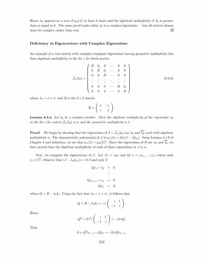
Hence (0 appears as a root of pA(() at least k times and the algebraic multiplicity of (0 is greaterthan or equal to k. The same proof works when (0 is a complex eigenvalue — but all vectors chosenmust be complex rather than real.

Deficiency in Eigenvectors with Complex Eigenvalues

An example of a real matrix with complex conjugate eigenvalues having geometric multiplicity lessthan algebraic multiplicity is the 2n" 2n block matrix

:Jn((0) =

!

"""""""""#

B I2 0 · · · 0 00 B I2 · · · 0 00 0 B · · · 0 0...

......

. . ....

...0 0 0 · · · B I2

0 0 0 · · · 0 B

$

%%%%%%%%%&

(8.3.3)

where (0 = * + i, and B is the 2" 2 matrix

B =

'* !,, *

(.

Lemma 8.3.4. Let (0 be a complex number. Then the algebraic multiplicity of the eigenvalue (0

in the 2n" 2n matrix :Jn((0) is n and the geometric multiplicity is 1.

Proof: We begin by showing that the eigenvalues of J = :Jn((0) are (0 and (0, each with algebraicmultiplicity n. The characteristic polynomial of J is pJ (() = det(J ! (I2n). From Lemma 4.1.9 ofChapter 4 and induction, we see that pJ (() = pB(()n. Since the eigenvalues of B are (0 and (0, wehave proved that the algebraic multiplicity of each of these eigenvalues in J is n.

Next, we compute the eigenvectors of J . Let Jv = (0v and let v = (v1, . . . , vn) where eachvj % C2. Observe that (J ! (0I2n)v = 0 if and only if

Qv1 + v2 = 0...

Qvn#1 + vn = 0

Qvn = 0,

where Q = B ! (0I2. Using the fact that (0 = * + i, , it follows that

Q = B ! (0I2 = !,'

i 1!1 i

(.

Hence

Q2 = 2,2i

'i 1!1 i

(= !2, iQ.

Thus0 = Q2vn#1 + Qvn = !2, iQvn#1,

272

from which it follows that Qvn#1 + vn = vn = 0. Similarly, v2 = · · · = vn#1 = 0. Since there is onlyone nonzero complex vector v1 (up to a complex scalar multiple) satisfying

Qv1 = 0,

it follows that the geometric multiplicity of (0 in the matrix :Jn((0) equals 1.

Definition 8.3.5. The real matrices Jn((0) when (0 % R and :Jn((0) when (0 % C are real Jordanblocks. The matrices Jn((0) when (0 % C are (complex) Jordan blocks.

Generalized Eigenvectors and Generalized Eigenspaces

What happens when n " n matrices have fewer that n linearly independent eigenvectors? Answer:The matrices gain generalized eigenvectors.

Definition 8.3.6. A vector v % Cn is a generalized eigenvector for the n"n matrix A with eigenvalue( if

(A ! (In)kv = 0 (8.3.4)

for some positive integer k. The smallest integer k for which (8.3.4) is satisfied is called the indexof the generalized eigenvector v.

Note: Eigenvectors are generalized eigenvectors with index equal to 1.

Let (0 be a real number and let N = Jn((0) ! (0In. Recall that (8.3.2) implies that Nn = 0.Hence every vector in Rn is a generalized eigenvector for the matrix Jn((0). So Jn((0) provides agood example of a matrix whose lack of eigenvectors (there is only one independent eigenvector) ismade up for by generalized eigenvectors (there are n independent generalized eigenvectors).

Let (0 be an eigenvalue of the n " n matrix A and let A0 = A ! (0In. For simplicity, assumethat (0 is real. Note that

null space(A0) 1 null space(A20) 1 · · · 1 null space(Ak

0) 1 · · · 1 Rn.

Therefore, the dimensions of the null spaces are bounded above by n and there must be a smallestk such that

dimnull space(Ak0) = dimnull space(Ak+1

0 ).

It follows thatnull space(Ak

0) = null space(Ak+10 ). (8.3.5)

Lemma 8.3.7. Let (0 be a real eigenvalue of the n " n matrix A and let A0 = A ! (0In. Let k bethe smallest integer for which (8.3.5) is valid. Then

null space(Ak0) = null space(Ak+j

0 )

for every interger j > 0.

273

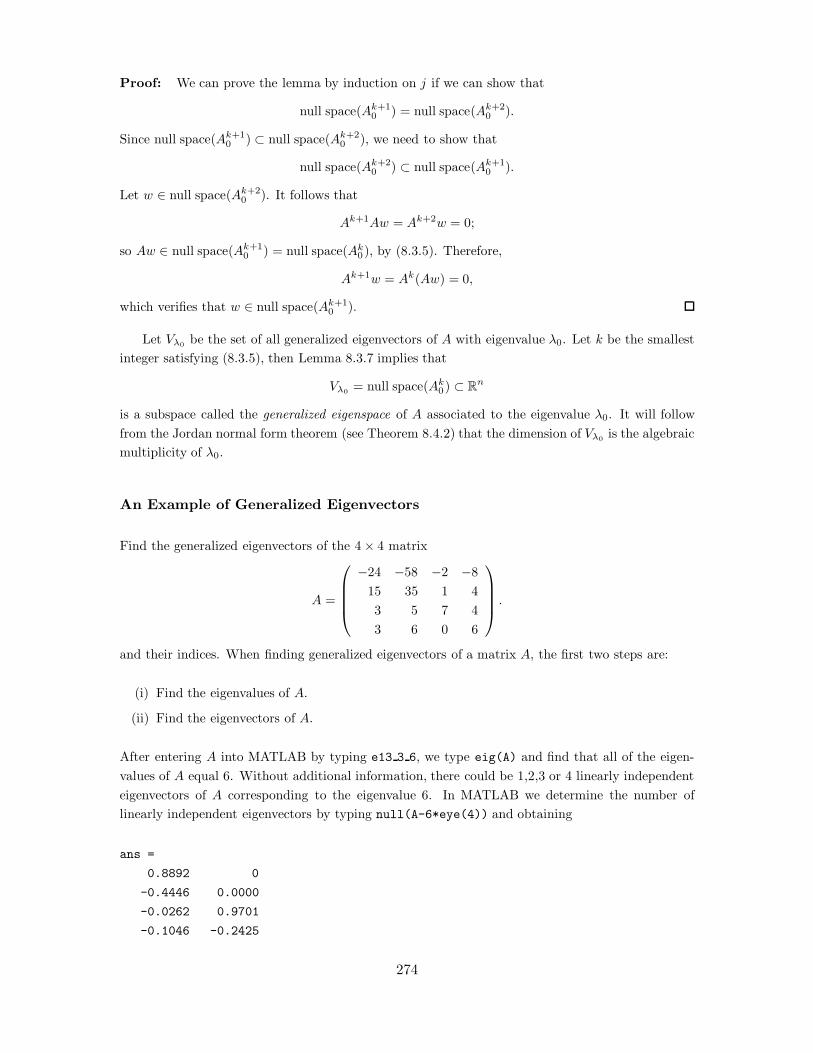
Proof: We can prove the lemma by induction on j if we can show that

null space(Ak+10 ) = null space(Ak+2

0 ).

Since null space(Ak+10 ) 1 null space(Ak+2

0 ), we need to show that

null space(Ak+20 ) 1 null space(Ak+1

0 ).

Let w % null space(Ak+20 ). It follows that

Ak+1Aw = Ak+2w = 0;

so Aw % null space(Ak+10 ) = null space(Ak

0), by (8.3.5). Therefore,

Ak+1w = Ak(Aw) = 0,

which verifies that w % null space(Ak+10 ).

Let V&0 be the set of all generalized eigenvectors of A with eigenvalue (0. Let k be the smallestinteger satisfying (8.3.5), then Lemma 8.3.7 implies that

V&0 = null space(Ak0) 1 Rn

is a subspace called the generalized eigenspace of A associated to the eigenvalue (0. It will followfrom the Jordan normal form theorem (see Theorem 8.4.2) that the dimension of V&0 is the algebraicmultiplicity of (0.

An Example of Generalized Eigenvectors

Find the generalized eigenvectors of the 4" 4 matrix

A =

!

"""#

!24 !58 !2 !815 35 1 43 5 7 43 6 0 6

$

%%%&.

and their indices. When finding generalized eigenvectors of a matrix A, the first two steps are:

(i) Find the eigenvalues of A.

(ii) Find the eigenvectors of A.

After entering A into MATLAB by typing e13 3 6, we type eig(A) and find that all of the eigen-values of A equal 6. Without additional information, there could be 1,2,3 or 4 linearly independenteigenvectors of A corresponding to the eigenvalue 6. In MATLAB we determine the number oflinearly independent eigenvectors by typing null(A-6*eye(4)) and obtaining

ans =

0.8892 0

-0.4446 0.0000

-0.0262 0.9701

-0.1046 -0.2425

274

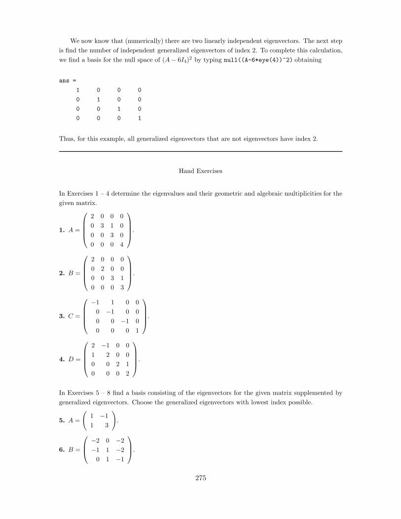
We now know that (numerically) there are two linearly independent eigenvectors. The next stepis find the number of independent generalized eigenvectors of index 2. To complete this calculation,we find a basis for the null space of (A! 6I4)2 by typing null((A-6*eye(4))^2) obtaining

ans =

1 0 0 0

0 1 0 0

0 0 1 0

0 0 0 1

Thus, for this example, all generalized eigenvectors that are not eigenvectors have index 2.

Hand Exercises

In Exercises 1 – 4 determine the eigenvalues and their geometric and algebraic multiplicities for thegiven matrix.

1. A =

!

"""#

2 0 0 00 3 1 00 0 3 00 0 0 4

$

%%%&.

2. B =

!

"""#

2 0 0 00 2 0 00 0 3 10 0 0 3

$

%%%&.

3. C =

!

"""#

!1 1 0 00 !1 0 00 0 !1 00 0 0 1

$

%%%&.

4. D =

!

"""#

2 !1 0 01 2 0 00 0 2 10 0 0 2

$

%%%&.

In Exercises 5 – 8 find a basis consisting of the eigenvectors for the given matrix supplemented bygeneralized eigenvectors. Choose the generalized eigenvectors with lowest index possible.

5. A =

'1 !11 3

(.

6. B =

!

"#!2 0 !2!1 1 !2

0 1 !1

$

%&.

275

7. C =

!

"#!6 31 !14!1 6 !2

0 2 1

$

%&.

8. D =

!

"#5 1 0!3 1 1!12 !4 0

$

%&.

Computer Exercises

In Exercises 9 – 10, use MATLAB to find the eigenvalues and their algebraic and geometric multi-plicities for the given matrix.

9.

A =

!

"""#

2 3 !21 !32 7 !41 !50 1 !5 !10 0 4 4

$

%%%&.

10.

B =

!

""""""#

179 !230 0 10 !30144 !185 0 8 !2430 !39 !1 3 !9

192 !245 0 9 !3040 !51 0 2 !7

$

%%%%%%&.

8.4 The Jordan Normal Form Theorem

The question that we discussed in Sections 8.1 and 8.2 is: Up to similarity, what is the simplestform that a matrix can have? We have seen that if A has real distinct eigenvalues, then A isreal diagonalizable. That is, A is similar to a diagonal matrix whose diagonal entries are the realeigenvalues of A. Similarly, if A has distinct real and complex eigenvalues, then A is complexdiagonalizable; that is, A is similar either to a diagonal matrix whose diagonal entries are the realand complex eigenvalues of A or to a real block diagonal matrix.

In this section we address the question of simplest form when a matrix has multiple eigenval-ues. In much of this discussion we assume that A is an n " n matrix with only real eigenvalues.Lemma 8.1.3 shows that if the eigenvectors of A form a basis, then A is diagonalizable. Indeed,for A to be diagonalizable, there must be a basis of eigenvectors of A. It follows that if A is notdiagonalizable, then A must have fewer than n linearly independent eigenvectors.

The prototypical examples of matrices having fewer eigenvectors than eigenvalues are the ma-trices Jn(() for ( real (see (8.3.1)) and :Jn(() for ( complex (see (8.3.3)).

276

Definition 8.4.1. A matrix is in Jordan normal form if it is block diagonal and the matrix in eachblock on the diagonal is a Jordan block, that is, J!(() for some integer # and some real or complexnumber (.

A matrix is in real Jordan normal form if it is block diagonal and the matrix in each block onthe diagonal is a real Jordan block, that is, either J!(() for some integer # and some real number (or :J!(() for some integer # and some complex number (.

The main theorem about Jordan normal form is:

Theorem 8.4.2 (Jordan normal form). Let A be an n"n matrix. Then A is similar to a Jordannormal form matrix and to a real Jordan normal form matrix.

This theorem is proved by constructing a basis V for Rn so that the matrix S#1AS is in Jordannormal form, where S is the matrix whose columns consists of vectors in V. The algorithm forfinding the basis V is complicated and is found in Appendix 8.6. In this section we construct V onlyin the special and simpler case where each eigenvalue of A is real and is associated with exactly oneJordan block.

More precisely, let (1, . . . ,(s be the distinct eigenvalues of A and let

Aj = A! (jIn.

The eigenvectors corresponding to (j are the vectors in the null space of Aj and the generalizedeigenvectors are the vectors in the null space of Ak

j for some k. The dimension of the null space ofAj is precisely the number of Jordan blocks of A associated to the eigenvalue (j . So the assumptionthat we make here is

nullity(Aj) = 1

for j = 1, . . . , s.

Let kj be the integer whose existence is specified by Lemma 8.3.7. Since, by assumption, there isonly one Jordan block associated with the eigenvalue (j , it follows that kj is the algebraic multiplicityof the eigenvalue (j .

To find a basis in which the matrix A is in Jordan normal form, we proceed as follows. First,let wjkj be a vector in

null space(Akj

j ) – null space(Akj#1j ).

Define the vectors wji by

wj,kj#1 = Ajwj,kj

...

wj,1 = Ajwj,2.

Second, when (j is real, let the kj vectors vji = wji, and when (j is complex, let the 2kj vectors vji

be defined by

vj,2i#1 = Re(wji)

vj,2i = Im(wji).

277

Let V be the set of vectors vji % Rn. We will show in Appendix 8.6 that the set V consists of n

vectors and is a basis of Rn. Let S be the matrix whose columns are the vectors in V. Then S#1AS

is in Jordan normal form.

The Cayley Hamilton Theorem

As a corollary of the Jordan normal form theorem, we prove the Cayley Hamilton theorem whichstates that a square matrix satisfies its characteristic polynomial . More precisely:

Theorem 8.4.3 (Cayley Hamilton). Let A be a square matrix and let pA(() be its characteristicpolynomial. Then

pA(A) = 0.

Proof: Let A be an n" n matrix. The characteristic polynomial of A is

pA(() = det(A ! (In).

Suppose that B = P#1AP is a matrix similar to A. Theorem 4.3.8 states that pB = pA. Therefore

pB(B) = pA(P#1AP ) = P#1pA(A)P.

So if the Cayley Hamilton theorem holds for a matrix similar to A, then it is valid for the matrix A.Moreover, using the Jordan normal form theorem, we may assume that A is in Jordan normal form.

Suppose that A is block diagonal, that is

A =

'A1 0

0 A2

(,

where A1 and A2 are square matrices. Then

pA(() = pA1 (()pA2(().

This observation follows directly from Lemma 4.1.9. Since

Ak =

'Ak

1 00 Ak

2

(,

it follows that

pA(A) =

'pA(A1) 0

0 pA(A2)

(=

'pA1(A1)pA2(A1) 0

0 pA1(A2)pA2(A2)

(.

It now follows from this calculation that if the Cayley Hamilton theorem is valid for Jordan blocks,then pA1(A1) = 0 = pA2(A2). So pA(A) = 0 and the Cayley Hamilton theorem is valid for allmatrices.

A direct calculation shows that Jordan blocks satisfy the Cayley Hamilton theorem. To begin,suppose that the eigenvalue of the Jordan block is real. Note that the characteristic polynomial ofthe Jordan block Jn((0) in (8.3.1) is (( ! (0)n. Indeed, Jn((0) ! (0In is strictly upper triangularand (Jn((0) ! (0In)n = 0. If (0 is complex, then either repeat this calculation using the complexJordan form or show by direct calculation that (A ! (0In)(A ! (0In) is strictly upper triangularwhen A = :Jn((0) is the real Jordan form of the Jordan block in (8.3.3).

278

An Example

Consider the 4" 4 matrix

A =

!

"""#

!147 !106 !66 !488604 432 271 1992621 448 279 2063!169 !122 !76 !562

$

%%%&.

Using MATLAB we can compute the characteristic polynomial of A by typing

poly(A)

The output is

ans =

1.0000 -2.0000 -15.0000 -0.0000 -0.0000

Note that since A is a matrix of integers we know that the coe!cients of the characteristic polynomialof A must be integers. Thus the characteristic polynomial is exactly:

pA(() = (4 ! 2(3 ! 15(2 = (2(( ! 5)(( + 3).

So (1 = 0 is an eigenvalue of A with algebraic multiplicity two and (2 = 5 and (3 = !3 are simpleeigenvalues of multiplicity one.

We can find eigenvectors of A corresponding to the simple eigenvalues by typing

v2 = null(A-5*eye(4));

v3 = null(A+3*eye(4));

At this stage we do not know how many linearly independent eigenvectors have eigenvalue 0. Thereare either one or two linearly independent eigenvectors and we determine which by typing null(A)

and obtaining

ans =

-0.1818

0.6365

0.7273

-0.1818

So MATLAB tells us that there is just one linearly independent eigenvector having 0 as an eigenvalue.There must be a generalized eigenvector in V0. Indeed, the null space of A2 is two dimensional andthis fact can be checked by typing

279

null2 = null(A^2)

obtaining

null2 =

0.2193 -0.2236

-0.5149 -0.8216

-0.8139 0.4935

0.1561 0.1774

Choose one of these vectors, say the first vector, to be v12 by typing

v12 = null2(:,1);

Since the algebraic multiplicity of the eigenvalue 0 is two, we choose the fourth basis vector bev11 = Av12. In MATLAB we type

v11 = A*v12

obtaining

v11 =

-0.1263

0.4420

0.5051

-0.1263

Since v11 is nonzero, we have found a basis for V0. We can now put the matrix A in Jordan normalform by setting

S = [v11 v12 v2 v3];

J = inv(S)*A*S

to obtain

J =

-0.0000 1.0000 0.0000 -0.0000

0.0000 0.0000 0.0000 -0.0000

-0.0000 -0.0000 5.0000 0.0000

0.0000 -0.0000 -0.0000 -3.0000

280

We have only discussed a Jordan normal form example when the eigenvalues are real and mul-tiple. The case when the eigenvalues are complex and multiple first occurs when n = 4. A samplecomplex Jordan block when the matrix has algebraic multiplicity two eigenvalues *±i, of geometricmultiplicity one is !

"""#

* !, 1 0, * 0 10 0 * !,0 0 , *

$

%%%& .

Numerical Di!culties

When a matrix has multiple eigenvalues, then numerical di!culties can arise when using the MAT-LAB command eig(A), as we now explain.

Let p(() = (2. Solving p(() = 0 is very easy — in theory — as ( = 0 is a double root of p.Suppose, however, that we want to solve p(() = 0 numerically. Then, numerical errors will lead tosolving the equation

(2 = +

where + is a small number. Note that if + > 0, the solutions are ±$+; while if + < 0, the solutions

are ±i.

|+|. Since numerical errors are machine dependent, + can be of either sign. The numericalprocess of finding double roots of a characteristic polynomial (that is, double eigenvalues of a matrix)is similar to numerically solving the equation (2 = 0, as we shall see.

For example, on a Sun SPARCstation 10 using MATLAB version 4.2c, the eigenvalues of the4" 4 matrix A in (8.4) (in format long) obtained using eig(A) are:

ans =

5.00000000001021

-0.00000000000007 + 0.00000023858927i

-0.00000000000007 - 0.00000023858927i

-3.00000000000993

That is, MATLAB computes two complex conjugate eigenvalues

±0.00000023858927i

which corresponds to an + of -5.692483975913288e-14. On a IBM compatible 486 computer usingMATLAB version 4.2 the same computation yields eigenvalues

ans=

4.99999999999164

0.00000057761008

-0.00000057760735

-2.99999999999434

281

That is, on this computer MATLAB computes two real, near zero, eigenvalues

±0.00000057761

that corresponds to an + of 3.336333121e-13. These errors are within round o" error in doubleprecision computation.

A consequence of these kinds of error, however, is that when a matrix has multiple eigenvalues,we cannot use the command [V,D] = eig(A) with confidence. On the Sun SPARCstation, thiscommand yields a matrix

V =

-0.1652 0.0000 - 0.1818i 0.0000 + 0.1818i -0.1642

0.6726 -0.0001 + 0.6364i -0.0001 - 0.6364i 0.6704

0.6962 -0.0001 + 0.7273i -0.0001 - 0.7273i 0.6978

-0.1888 0.0000 - 0.1818i 0.0000 + 0.1818i -0.1915

that suggests that A has two complex eigenvectors corresponding to the ‘complex’ pair of near zeroeigenvalues. The IBM compatible yields the matrix

V =

-0.1652 0.1818 -0.1818 -0.1642

0.6726 -0.6364 0.6364 0.6704

0.6962 -0.7273 0.7273 0.6978

-0.1888 0.1818 -0.1818 -0.1915

indicating that MATLAB has found two real eigenvectors corresponding to the near zero real eigen-values. Note that the two eigenvectors corresponding to the eigenvalues 5 and !3 are correct onboth computers.

Hand Exercises

1. Write two di"erent 4" 4 Jordan normal form matrices all of whose eigenvalues equal 2 for whichthe geometric multiplicity is two.

2. How many di"erent 6"6 Jordan form matrices have all eigenvalues equal to 3? (We say that twoJordan form matrices are the same if they have the same number and type of Jordan block, thoughnot necessarily in the same order along the diagonal.)

3. A 5 " 5 matrix A has three eigenvalues equal to 4 and two eigenvalues equal to !3. List thepossible Jordan normal forms for A (up to similarity). Suppose that you can ask your computer tocompute the nullity of precisely two matrices. Can you devise a strategy for determining the Jordannormal form of A? Explain your answer.

282

4. An 8" 8 real matrix A has three eigenvalues equal to 2, two eigenvalues equal to 1 + i, and onezero eigenvalue. List the possible Jordan normal forms for A (up to similarity). Suppose that youcan ask your computer to compute the nullity of precisely two matrices. Can you devise a strategyfor determining the Jordan normal form of A? Explain your answer.

In Exercises 5 – 10 find the Jordan normal forms for the given matrix.

5. A =

'2 41 1

(.

6. B =

'9 25!4 !11

(.

7. C =

!

"#!5 !8 !9

5 9 9!1 !2 !1

$

%&.

8. D =

!

"#0 1 00 0 11 1 !1

$

%&.

9. E =

!

"#2 0 !12 1 !11 0 0

$

%&.

10. F =

!

"#3 !1 2!1 2 !1!1 1 0

$

%&.

11. Compute etJ where J =

!

"#2 0 00 !1 10 0 !1

$

%&.

12. Compute etJ where J =

!

""""""#

2 1 0 0 00 2 0 0 00 0 3 1 00 0 0 3 10 0 0 0 3

$

%%%%%%&.

13. An n" n matrix N is nilpotent if Nk = 0 for some positive integer k.

(a) Show that the matrix N defined in (8.3.2) is nilpotent.

(b) Show that all eigenvalues of a nilpotent matrix equal zero.

(c) Show that any matrix similar to a nilpotent matrix is also nilpotent.

(d) Let N be a matrix all of whose eigenvalues are zero. Use the Jordan normal form theorem toshow that N is nilpotent.

283

14. Let A be a 3 " 3 matrix. Use the Cayley-Hamilton theorem to show that A#1 is a linearcombination of I3, A, A2. That is, there exist real scalars a, b, c such that

A#1 = aI3 + bA + cA2.

Computer Exercises

In Exercises 15 – 19, (a) determine the real Jordan normal form for the given matrix A, and (b) findthe matrix S so that S#1AS is in real Jordan normal form.

15.

A =

!

"""#

!3 !4 !2 0!9 !39 !16 !718 64 27 1015 86 34 18

$

%%%&.

16.

A =

!

"""#

9 45 18 80 !4 !1 !1

!16 !69 !29 !1225 123 49 23

$

%%%& .

17.

A =

!

"""#

!5 !13 17 42!10 !57 66 187!4 !23 26 77!1 !9 9 32

$

%%%&.

18.

A =

!

"""#

1 0 !9 1812 !7 !26 775 !2 !13 322 !1 !4 11

$

%%%& .

19.

A =

!

"""#

!1 !1 1 0!3 1 1 0!3 2 !1 1!3 2 0 0

$

%%%&.

20.

A =

!

""""""#

0 0 !1 2 21 !2 0 2 21 !1 !1 2 20 0 0 1 20 0 0 !1 3

$

%%%%%%&.

284

8.5 *Appendix: Markov Matrix Theory

In this appendix we use the Jordan normal form theorem to study the asymptotic dynamics oftransition matrices such as those of Markov chains introduced in Section 4.5.

The basic result is the following theorem.

Theorem 8.5.1. Let A be an n" n matrix and assume that all eigenvalues ( of A satisfy |(| < 1.Then for every vector v0 % Rn

limk&'

Akv0 = 0. (8.5.1)

Proof: Suppose that A and B are similar matrices; that is, B = SAS#1 for some invertible matrixS. Then Bk = SAkS#1 and for any vector v0 % Rn (8.5.1) is valid if and only if

limk&'

Bkv0 = 0.

Thus, when proving this theorem, we may assume that A is in Jordan normal form.

Suppose that A is in block diagonal form; that is, suppose

A =

'C 00 D

(,

where C is an #" # matrix and D is a (n! #) " (n ! #) matrix. Then

Ak =

'Ck 0

0 Dk

(.

So for every vector v0 = (w0, u0) % R! "Rn#! (8.5.1) is valid if and only if

limk&'

Ckv0 = 0 and limk&'

Dkv0 = 0.

So, when proving this theorem, we may assume that A is a Jordan block.

Consider the case of a simple Jordan block. Suppose that n = 1 and that A = (() where ( iseither real or complex. Then

Akv0 = (kv0.

It follows that (8.5.1) is valid precisely when |(| < 1. Next, suppose that A is a nontrivial Jordanblock. For example, let

A =

'( 10 (

(= (I2 + N

where N2 = 0. It follows by induction that

Akv0 = (kv0 + k(k#1Nv0 = (kv0 + k(k 1(

Nv0.

Thus (8.5.1) is valid precisely when |(| < 1. The reason for this convergence is as follows. The firstterm converges to 0 as before but the second term is the product of three terms k, (k, and 1

&Nv0.

285

The first increases to infinity, the second decreases to zero, and the third is constant independent ofk. In fact, geometric decay ((k, when |(| < 1) always beats polynomial growth. Indeed,

limm&'

mj(m = 0 (8.5.2)

for any integer j. This fact can be proved using l’Hospital’s rule and induction.

So we see that when A has a nontrivial Jordan block, convergence is subtler than when A hasonly simple Jordan blocks, as initially the vectors Av0 grow in magnitude. For example, supposethat ( = 0.75 and v0 = (1, 0)t. Then A8v0 = (0.901, 0.075)t is the first vector in the sequence Akv0

whose norm is less than 1; that is, A8v0 is the first vector in the sequence closer to the origin thanv0.

It is also true that (8.5.1) is valid for any Jordan block A and for all v0 precisely when |(| < 1.To verify this fact we use the binomial theorem. We can write a nontrivial Jordan block as (In + N

where Nk+1 = 0 for some integer k. We just discussed the case k = 1. In this case

((In + N )m = (mIn + m(m#1N +

'm

2

((m#2N2 + · · ·+

'm

k

((m#kNk,

where 'm

j

(=

m!j!(m ! j)!

=m(m ! 1) · · · (m! j + 1)

j!.

To verify thatlim

m&'((In + N )m = 0

we need only verify that each term

limm&'

'm

j

((m#jN j = 0

Such terms are the product of three terms

m(m ! 1) · · · (m ! j + 1) and (m and1

j!(jN j .

The first term has polynomial growth to infinity dominated by mj , the second term decreases tozero geometrically, and the third term is constant independent of m. The desired convergence tozero follows from (8.5.2).

Definition 8.5.2. The n"n matrix A has a dominant eigenvalue (0 > 0 if (0 is a simple eigenvalueand all other eigenvalues ( of A satisfy |(| < (0.

Theorem 8.5.3. Let P be a Markov matrix. Then 1 is a dominant eigenvalue of P .

Proof: Recall from Chapter 3, Definition 4.5.1 that a Markov matrix is a square matrix P whoseentries are nonnegative, whose rows sum to 1, and for which a power P k that has all positive entries.To prove this theorem we must show that all eigenvalues ( of P satisfy |(| ( 1 and that 1 is a simpleeigenvalue of P .

286

Let ( be an eigenvalue of P and let v = (v1, . . . , vn)t be an eigenvector corresponding to theeigenvalue (. We prove that |(| ( 1. Choose j so that |vj | ' |vi| for all i. Since Pv = (v, we canequate the jth coordinates of both sides of this equality, obtaining

pj1v1 + · · ·+ pjnvn = (vj.

Therefore,|(||vj| = |pj1v1 + · · ·+ pjnvn| ( pj1|v1| + · · ·+ pjn|vn|,

since the pij are nonnegative. It follows that

|(||vj| ( (pj1 + · · ·+ pjn)|vj | = |vj|,

since |vi| ( |vj| and rows of P sum to 1. Since |vj| > 0, it follows that ( ( 1.

Next we show that 1 is a simple eigenvalue of P . Recall, or just calculate directly, that the vector(1, . . . , 1)t is an eigenvector of P with eigenvalue 1. Now let v = (v1, . . . , vn)t be an eigenvector of P

with eigenvalue 1. Let Q = P k so that all entries of Q are positive. Observe that v is an eigenvectorof Q with eigenvalue 1, and hence that all rows of Q also sum to 1.

To show that 1 is a simple eigenvalue of Q, and therefore of P , we must show that all coordinatesof v are equal. Using the previous estimates (with ( = 1), we obtain

|vj | = |qj1v1 + · · ·+ qjnvn| ( qj1|v1| + · · ·+ qjn|vn| ( |vj|. (8.5.3)

Hence|qj1v1 + · · ·+ qjnvn| = qj1|v1| + · · ·+ qjn|vn|.

This equality is valid only if all of the vi are nonnegative or all are nonpositive. Without loss ofgenerality, we assume that all vi ' 0. It follows from (8.5.3) that

vj = qj1v1 + · · ·+ qjnvn.

Since qji > 0, this inequality can hold only if all of the vi are equal.

Theorem 8.5.4. (a) Let Q be an n " n matrix with dominant eigenvalue ( > 0 and associatedeigenvector v. Let v0 be any vector in Rn. Then

limk&'

1(k

Qkv0 = cv,

for some scalar c.

(b) Let P be a Markov matrix and v0 a nonzero vector in Rn with all entries nonnegative. Then

limk&'

(P t)kv0 = V

where V is the eigenvector of P t with eigenvalue 1 such that the sum of the entries in V is equal tothe sum of the entries in v0.

Proof: (a) After a similarity transformation, if needed, we can assume that Q is in Jordan normalform. More precisely, we can assume that

1(

Q =

'1 00 A

(

287

where A is an (n ! 1) " (n ! 1) matrix with all eigenvalues µ satisfying |µ| < 1. Suppose v0 =(c0, w0) % R "Rn#1. It follows from Theorem 8.5.1 that

limk&'

1(k

Qkv0 = limk&'

(1(

Q)kv0 = limk&'

'c0 00 Akw0

(= c0e1.

Since e1 is the eigenvector of Q with eigenvalue ( Part (a) is proved.

(b) Theorem 8.5.3 states that a Markov matrix has a dominant eigenvalue equal to 1. TheJordan normal form theorem implies that the eigenvalues of P t are equal to the eigenvalues of P

with the same algebraic and geometric multiplicities. It follows that 1 is also a dominant eigenvalueof P t. It follows from Part (a) that

limk&'

(P t)kv0 = cV

for some scalar c. But Theorem 4.5.3 in Chapter 3 implies that the sum of the entries in v0 equals thesum of the entries in cV which, by assumption equals the sum of the entries in V . Thus, c = 1.

Hand Exercises

1. Let A be an n " n matrix. Suppose that

limk&'

Akv0 = 0.

for every vector v0 % Rn. Then the eigenvalues ( of A all satisfy |(| < 1.

8.6 *Appendix: Proof of Jordan Normal Form

We prove the Jordan normal form theorem under the assumption that the eigenvalues of A are allreal. The proof for matrices having both real and complex eigenvalues proceeds along similar lines.

Let A be an n"n matrix, let (1, . . . ,(s be the distinct eigenvalues of A, and let Aj = A!(jIn.

Lemma 8.6.1. The linear mappings Ai and Aj commute.

Proof: Just compute

AiAj = (A! (iIn)(A! (jIn) = A2 ! (iA ! (jA + (i(jIn,

andAjAi = (A! (jIn)(A ! (iIn) = A2 ! (jA ! (iA + (j(iIn.

So AiAj = AjAi, as claimed.

Let Vj be the generalized eigenspace corresponding to eigenvalue (j .

Lemma 8.6.2. Ai : Vj * Vj is invertible when i #= j.

288

Proof: Recall from Lemma 8.3.7 that Vj = null space(Akj ) for some k ' 1. Suppose that v % Vj.

We first verify that Aiv is also in Vj . Using Lemma 8.6.1, just compute

Akj Aiv = AiA

kj v = Ai0 = 0.

Therefore, Aiv % null space(Akj ) = Vj .

Let B be the linear mapping Ai|Vj . It follows from Chapter 6, Theorem 6.2.3 that

nullity(B) + dimrange(B) = dim(Vj).

Now w % null space(B) if w % Vj and Aiw = 0. Since Aiw = (A ! (iIn)w = 0, it follows thatAw = (iw. Hence

Ajw = (A ! (jIn)w = ((i ! (j)w

andAk

j w = ((i ! (j)kw.

Since (i #= (j , it follows that Akj w = 0 only when w = 0. Hence the nullity of B is zero. We conclude

thatdimrange(B) = dim(Vj).

Thus, B is invertible, since the domain and range of B are the same space.

Lemma 8.6.3. Nonzero vectors taken from di!erent generalized eigenspaces Vj are linearly inde-pendent. More precisely, if wj % Vj and

w = w1 + · · ·+ ws = 0,

then wj = 0.

Proof: Let Vj = null space(Akj

j ) for some integer kj. Let C = Ak22 " · · · "Aks

s . Then

0 = Cw = Cw1,

since Akj

j wj = 0 for j = 2, . . . , s. But Lemma 8.6.2 implies that C|V1 is invertible. Therefore,w1 = 0. Similarly, all of the remaining wj have to vanish.

Lemma 8.6.4. Every vector in Rn is a linear combination of vectors in the generalized eigenspacesVj .

Proof: Let W be the subspace of Rn consisting of all vectors of the form z1 + · · · + zs wherezj % Vj. We need to verify that W = Rn. Suppose that W is a proper subspace. Then choose abasis w1, . . . , wt of W and extend this set to a basis W of Rn. In this basis the matrix [A]W hasblock form, that is,

[A]W =

'A11 A12

0 A22

(,

where A22 is an (n ! t) " (n! t) matrix. The eigenvalues of A22 are eigenvalues of A. Since all ofthe distinct eigenvalues and eigenvectors of A are accounted for in W (that is, in A11), we have acontradiction. So W = Rn, as claimed.

289

Lemma 8.6.5. Let Vj be a basis for the generalized eigenspaces Vj and let V be the union of thesets Vj . Then V is a basis for Rn.

Proof: We first show that the vectors in V span Rn. It follows from Lemma 8.6.4 that everyvector in Rn is a linear combination of vectors in Vj . But each vector in Vj is a linear combinationof vectors in Vj . Hence, the vectors in V span Rn.

Second, we show that the vectors in V are linearly independent. Suppose that a linear combi-nation of vectors in V sums to zero. We can write this sum as

w1 + · · ·+ ws = 0,

where wj is the linear combination of vectors in Vj . Lemma 8.6.3 implies that each wj = 0. SinceVj is a basis for Vj , it follows that the coe!cients in the linear combinations wj must all be zero.Hence, the vectors in V are linearly independent.

Finally, it follows from Theorem 5.5.3 of Chapter 5 that V is a basis.

Lemma 8.6.6. In the basis V of Rn guaranteed by Lemma 8.6.5, the matrix [A]V is block diagonal,that is,

[A]V =

!

""#

A11 0 0

0. . . 0

0 0 Ass

$

%%& ,

where all of the eigenvalues of Ajj equal (j.

Proof: It follows from Lemma 8.6.1 that A : Vj * Vj. Suppose that vj % Vj . Then Avj is in Vj

and Avj is a linear combination of vectors in Vj . The block diagonalization of [A]V follows. SinceVj = null space(Akj

j ), it follows that all eigenvalues of Ajj equal (j.

Lemma 8.6.6 implies that to prove the Jordan normal form theorem, we must find a basis inwhich the matrix Ajj is in Jordan normal form. So, without loss of generality, we may assume thatall eigenvalues of A equal (0, and then find a basis in which A is in Jordan normal form. Moreover,we can replace A by the matrix A ! (0In, a matrix all of whose eigenvalues are zero. So, withoutloss of generality, we assume that A is an n " n matrix all of whose eigenvalues are zero. We nowsketch the remainder of the proof of Theorem 8.4.2.

Let k be the smallest integer such that Rn = null space(Ak) and let

s = dimnull space(Ak)! dimnull space(Ak#1) > 0.

Let z1, . . . , zn#s be a basis for null space(Ak#1) and extend this set to a basis for null space(Ak) byadjoining the linearly independent vectors w1, . . . , ws. Let

Wk = span{w1, . . . , ws}.

It follows that Wk 0 null space(Ak#1) = {0}.

We claim that the ks vectors W = {wj! = A!(wj)} where 0 ( # ( k ! 1 and 1 ( j ( s arelinearly independent. We can write any linear combination of the vectors in W as yk + · · · + y1,

290

where yj % Ak#j(Wk). Suppose that

yk + · · ·+ y1 = 0.

Then Ak#1(yk + · · · + y1) = Ak#1yk = 0. Therefore, yk is in Wk and in null space(Ak#1). Hence,yk = 0. Similarly, Ak#2(yk#1 + · · · + y1) = Ak#2yk#1 = 0. But yk#1 = Ayk where yk % Wk andyk % null space(Ak#1). Hence, yk = 0 and yk#1 = 0. Similarly, all of the yj = 0. It follows fromyj = 0 that a linear combination of the vectors Ak#j(w1), . . . , Ak#j(ws) is zero; that is

0 = %1Ak#j(w1) + · · ·+ %sA

k#j(ws) = Ak#j(%1w1 + · · ·+ %sws).

Applying Aj#1 to this expression, we see that

%1w1 + · · ·+ %sws

is in Wk and in the null space(Ak#1). Hence,

%1w1 + · · ·+ %sws = 0.

Since the wj are linearly independent, each %j = 0, thus verifying the claim.

Next, we find the largest integer m so that

t = dimnull space(Am)! dim null space(Am#1) > 0.

Proceed as above. Choose a basis for null space(Am#1) and extend to a basis for null space(Am)by adjoining the vectors x1, . . . , xt. Adjoin the mt vectors A!xj to the set V and verify that thesevectors are all linearly independent. And repeat the process. Eventually, we arrive at a basis forRn = null space(Ak).

In this basis the matrix [A]V is block diagonal; indeed, each of the blocks is a Jordan block, since

A(wj!) =

9wj(!#1) 0 < # ( k ! 1

0 # = 1.

Note the resemblance with (8.3.2).

291

MATLAB Commands

† indicates an laode toolbox command not found in MATLAB

Chapter 1: Preliminaries

Editing and Number Commands

quit Ends MATLAB session; (a) At end of line the semicolon suppresses echo printing

(b) When entering an array the semicolon indicates a new row6 Displays previous MATLAB command[] Brackets indicating the beginning and the end of a vector or a matrixx=y Assigns x the value of yx(j) Recalls jth entry of vector x

A(i,j) Recalls ith row, jth column of matrix A

A(i,:) Recalls ith row of matrix A

A(:,j) Recalls jth column of matrix A

Vector Commands

norm(x) The norm or length of a vector x

dot(x,y) Computes the dot product of vectors x and y

†addvec(x,y) Graphics display of vector addition in the plane†addvec3(x,y) Graphics display of vector addition in three dimensions

Matrix Commands

A! (Conjugate) transpose of matrixzeros(m,n) Creates an m" n matrix all of whose entries equal 0zeros(n) Creates an n" n matrix all of whose entries equal 0diag(x) Creates an n" n diagonal matrix whose diagonal entries

are the components of the vector x % Rn

eye(n) Creates an n" n identity matrix

292

Special Numbers in MATLAB

pi The number " = 3.1415 . . .

acos(a) The inverse cosine of the number a

Chapter 2: Solving Linear Equations

Editing and Number Commands

format Changes the numbers display format to standard five digit formatformat long Changes display format to 15 digitsformat rational Changes display format to rational numbersformat short e Changes display to five digit floating point numbers

Vector Commands

x.*y Componentwise multiplication of the vectors x and y

x./y Componentwise division of the vectors x and y

x.^y Componentwise exponentiation of the vectors x and y

Matrix Commands

A([i j],:) = A([j i],:)

Swaps ith and jth rows of matrix A

A\b Solves the system of linear equations associated withthe augmented matrix (A|b)

x = linspace(xmin,xmax,N)

Generates a vector x whose entries are N equally spaced pointsfrom xmin to xmax

x = xmin:xstep:xmax

Generates a vector whose entries are equally spaced points from xmin to xmax

with stepsize xstep

[x,y] = meshgrid(XMIN:XSTEP:XMAX,YMIN:YSTEP:YMAX);

Generates two vectors x and y. The entries of x are values from XMIN to XMAX

in steps of XSTEP. Similarly for y.rand(m,n) Generates an m " n matrix whose entries are randomly and uniformly chosen

from the interval [0, 1]rref(A) Returns the reduced row echelon form of the m" n matrix A

the matrix after each step in the row reduction processrank(A) Returns the rank of the m" n matrix A

Graphics Commands

293

plot(x,y) Plots a graph connecting the points (x(i), y(i)) in sequencexlabel(’labelx’) Prints labelx along the x axisylabel(’labely’) Prints labely along the y axissurf(x,y,z) Plots a three dimensional graph of z(j) as a function of x(j) and y(j)hold on Instructs MATLAB to add new graphics to the previous figurehold off Instructs MATLAB to clear figure when new graphics are generatedgrid Toggles grid lines on a figureaxis(’equal’) Forces MATLAB to use equal x and y dimensionsview([a b c]) Sets viewpoint from which an observer sees the current 3-D plotzoom Zoom in and out on 2-D plot. On each mouse click, axes change by a factor of 2

Special Numbers and Functions in MATLAB

exp(x) The number ex where e = exp(1) = 2.7182 . . .

sqrt(x) The number$

x

i The number$!1

Chapter 3: Matrices and Linearity

Matrix Commands

A*x Performs the matrix vector product of the matrix A with the vector x

A*B Performs the matrix product of the matrices A and B

size(A) Determines the numbers of rows and columns of a matrix A

inv(A) Computes the inverse of a matrix A

Program for Matrix Mappings

†map Allows the graphic exploration of planar matrix mappings

Special Functions in MATLAB

sin(x) The number sin(x)cos(x) The number cos(x)

Matrix Commands

eig(A) Computes the eigenvalues of the matrix A

null(A) Computes the solutions to the homogeneous equation Ax = 0

294

Chapter 4: Determinants and Eigenvalues

Matrix Commands

det(A) Computes the determinant of the matrix A

poly(A) Returns the characteristic polynomial of the matrix A

sum(v) Computes the sum of the components of the vector v

trace(A) Computes the trace of the matrix A

[V,D] = eig(A) Computes eigenvectors and eigenvalues of the matrix A

Chapter 6: Linear Maps and Changes of Coordinates

Vector Commands

†bcoord Geometric illustration of planar coordinates by vector addition†ccoord Geometric illustration of coordinates relative to two bases

Chapter 7: Orthogonality

Matrix Commands

orth(A) Computes an orthonormal basis for the column space of the matrix A

[Q,R] = qr(A,0) Computes the QR decomposition of the matrix A

Graphics Commands

axis([xmin,xmax,ymin,ymax])

Forces MATLAB to use in a twodimensional plot the intervals[xmin,xmax] resp. [ymin,ymax] labeling the x- resp. y-axis

plot(x,y,’o’) Same as plot but now the points (x(i), y(i)) are marked bycircles and no longer connected in sequence

Matrix Commands

[V,D] = eig(A) Computes eigenvectors and eigenvalues of the matrix A

Chapter 8: Matrix Normal Forms

Vector Commands

real(v) Returns the vector of the real parts of the componentsof the vector v

imag(v) Returns the vector of the imaginary parts of the componentsof the vector v

295

Answers to Selected

Odd-Numbered Problems

Chapter 1: Preliminaries

Section 1.1: Vectors and Matrices

1 (3, 2, 2) 3 (1,!1, 9) 5 (5, 0) 7 not possible 9 not possible 11

'4 !4

!11 11

(

Section 1.2: MATLAB

1 (a) 11; (b)

!

"#153

24

$

%&; (c) (!6,!2,!6,!4); (d)

!

"#150

18

$

%&

3 (23.1640,!3.5620,!12.8215) 5

'!14.0300 !5.8470 7.0600!9.7600 11.0570 !9.6600

(

Section 1.3: Special Kinds of Matrices

1 symmetric 3 symmetric 5 symmetric 7 strictly upper triangular 9 not upper triangular 11 3 13mn 15 n(n+1)

2 17 true 19 false 21 At = (3)

Section 1.4: The Geometry of Vector Operations

1 ||x|| = 3 3 ||x|| =$

3 5 perpendicular 7 not perpendicular 9 a = 103 11 x · y = 4; cos ! = 2$

513

x · y = 13; cos ! = 136$

515 x · y = 31; cos ! = 31$

1410. 0.8256

Chapter 2: Solving Linear Equations

Section 2.1: Systems of Linear Equations and Matrices

1 (x, y) = (2, 4) 3 (x, y) = (!4, 1) 5 (a) has an infinite number of solutions; (b) has no solutions. 7(a) p(x) = !x2 + 5x + 1 11

296

ans =

-12.0495

-0.8889

7.8384

Section 2.2 The Geometry of Low-Dimensional Solutions

1 2x + 3y + z = !5 3 z = x 5 (a) u = (2, 2, 1) (b) v = (1, 1, 2) (c) cos ! = 2$6; ! = 35.2644". 7

(x, y) . (2.15,!1.54) 9 (x, y, z) = (1, 3,!1) 11 The function has three relative maxima.

Section 2.3: Gaussian Elimination

1 not in reduced echelon form 3 not in reduced echelon form 5 The 1st, 3rd, and 5th columns containpivots. The system is inconsistent; no solutions. 9 inconsistent; no solutions 11 (a) Infinitely manysolutions; (b) one variable can be assigned arbitrary values. 13 unique solution 15 linear 17 notlinear 19 not linear 21 consistent

23 The row echelon form is:

A =

0 1.0000 2.0000 1.0000 14.0000 21.0000 0 -1.0000

0 0 0 1.0000 3.0000 5.0000 0 9.0000

0 0 0 0 1.0000 -0.5000 0 -4.7143

0 0 0 0 0 1.0000 0 0.3457

0 0 0 0 0 0 0 1.0000

0 0 0 0 0 0 0 0

Section 2.4 Reduction to Echelon Form

1 The reduced echelon form of the matrix A is

!

"#1 2 0 40 0 1 20 0 0 0

$

%&; rank(A) = 2.

3 four 5 consistent; three parameters 7 inconsistent 9 1 11 2

Section 2.5 Linear Equations with Special Coe!cients

1

'x1

x2

(=

'32 !

12i

!12 !

12i

(3

'x1

x2

(=

'12

!12

(5

A\b =

0.3006+ 0.2462i

-0.6116+ 0.0751i

Chapter 3: Matrices and Linearity

297

Section 3.1: Matrix Multiplication of Vectors

1 (4, !11) 3 (6, !10) 5 (13) 9

'2 3 !26 0 !5

( !

"#x1

x2

x3

$

%& =

'41

(11 A =

'3 1!5 4

(13 No

upper triangular matrix satisfies (3.1.6), but any symmetric matrix of the form

'1 22 a22

(satisfies

(3.1.6). 15

b =

103.5000

175.8000

-296.9000

-450.1000

197.4000

656.6000

412.4000

17

A\b =

-2.3828

-1.0682

0.1794

Section 3.2: Matrix Mappings

1 (x1, 0)t 3 (x1, 3x1)t 5 R(#45!) =

'1$2

1$2

! 1$2

1$2

(7

'1 00 !1

(9

'0 11 0

(11 R90! =

'0 !11 0

(

15 A maps x = (1, 1)t to twice its length and x = s(0, 1)t to half its length. 17 C maps x = (1, 0) totwice its length and x = (1, 2) to !1

2 times its length. 19 Matrix B rotates the plane by ! =. 3.0585counterclockwise and dilatates it by a factor of c =

$5.8 . 2.4083. 21 A rotates the plane 30" clock-

wise. 23 C reflects the plane across the line y = x. 25 E maps (x, y) to a point on the line y = x;that point is (x+y

2 , x+y2 ).

Section 3.3: Linearity

1 (a) (!5, 11); (b) (6, 8,!16); (c) (21, 7,!10,!2) 3 $ = !75 ; % = !3

5 5 $ = 513& + 7

13 and

% = !1413& !

413 7 not linear 9 not linear 11 A =

!

"#0 !1 !11 0 21 !2 0

$

%& 13 A =

!

"#0 1 00 0 11 0 0

$

%& 17

The mapping rotates a 2-vector 90" clockwise and then it halves its length.

Section 3.4: The Principle of Superposition

298

1 (a) v1 =

!

"#!1

10

$

%& ; v2 =

!

"#!1

01

$

%& (b) w1 =

!

"#10!1

$

%& ; w2 =

!

"#01!1

$

%&

3 (a) s

!

"#!11

71

$

%&; (b)

!

"#111

$

%&; (c)

!

"#111

$

%& + s

!

"#!11

71

$

%&

Section 3.5: Composition and Multiplication of Matrices

1 AB =

'!2 0

7 !1

(; BA =

'!2 0

5 !1

(3 Neither AB nor BA is defined. 5

'!11 8!3 2

(

7

!

"#!4 13 3!12 11 !11

3 !1 4

$

%& 9 B =

'b11 0

0 b22

(11

!

"#10 !5 15!5 6 !415 !4 26

$

%& 13 Neither AB nor BA is

defined.

Section 3.6: Properties of Matrix Multiplication

3 B =

!

"#1 1 1

2

0 1 10 0 1

$

%&; C =

!

"#1 t t2

2

0 1 t

0 0 1

$

%&

Section 3.7: Solving Linear Systems and Inverses

3 a #= 0 and b #= 0 5 A#1 =110

!

"#!8 32 !9

2 2 12 !8 1

$

%& 9 A is invertible for any a, b, and c, and

A#1 =

!

"#1 !a !b + ac

0 1 !c

0 0 1

$

%&.

11 Type N = [B eye(4)] in MATLAB and then row reduce N to obtain

ans =

1.0000 0 0 0 -1.5714 -0.4286 0 1.4286

0 1.0000 0 0 0.7429 0.0571 0.2000 -0.4571

0 0 1.0000 0 -0.9143 0.3143 -0.4000 0.4857

0 0 0 1.0000 -0.6000 -0.2000 -0.2000 0.6000

Section 3.8: Determinants of 2" 2 Matrices

1

'2 !1!3 2

(9 y = 29

11 11 A is invertible; det(A) = 4. 13 A is not invertible; det(A) = 0

Chapter 5: Vector Spaces

299

Section 5.1: Vector Spaces and Subspaces

3 V1 and V3 are identical. 5 not a subspace 7 subspace 9 subspace 11 not a subspace 13 subspace15 not a subspace 17 subspace when c = 0; not a subspace when c #= 0

Section 5.2: Construction of Subspaces

1 span{(1, 0,!4)t, (0, 1, 2)t} 3 span{(1, 0,!1)t, (0, 1,!1)t}

5 span{(!2, 1, 0, 0, 0)t, (!1, 0,!4, 1, 0)t} 7 span{(!2,!1, 1)t} 9

'1 1 0 00 0 1 1

(11 (2, 20, 0)t =

!4w1 + 6w2 13 t4 #%W 15 y(t) = 0.5t2 %W , but {y(t), x2(t)} does not span W .

Section 5.3: Spanning Sets and MATLAB

1 span{(0.3225, 0.8931,!0.0992,0.2977)t, (0,!0.1961, 0.5883,0.7845)t}

3 span{(!0.8452,!0.1690, 0.5071)t}. 5 span{(!1,!3, 1, 0)t, (3/4, 2, 0, 1)t} 7 v2 #%W

Section 5.4: Linear Dependence and Linear Independence

3 linearly dependent. 9 linearly dependent

Section 5.5: Dimension and Bases

3 {(1, 1, 1, 0), (!2,!2, 0, 1)} is a basis; the dimension is two. 5 dimP2 = 3; dimPn = n + 1

Section 5.6: The Proof of the Main Theorem

1 A plane with N = n3(!32 , 1, 1). 3 A plane with N = n3(0, 0, 1). 5 (a) 5; (c) 5! r; (d) 5! r 9 (a)

( #= 2; (b) ( = 2 11 {(1, 0, 0,!12 , 3

2 ), (0, 1, 0, 12 ,!1

2 ), (0, 0, 1, 12 , 3

2 )}

Chapter 4: Determinants and Eigenvalues

Section 4.1: Determinants

1 !28 3 14 7 !4 9 (a) 1 and !1/3; (b) yes

13 B11 =

!

"#7 !2 100 0 !14 2 !10

$

%&; B23 =

!

"#0 2 50 0 !13 4 !10

$

%&; B43 =

!

"#0 2 5!1 7 10

0 0 !1

$

%&

Section 4.3: Eigenvalues

1 pA(() = !(3 + 2(2 + ( ! 2; the eigenvalues are 1, !1, and 2. 3 {(!1, 1, 0)t, (1, 0, 1)t} 5 (a) Theeigenvalues are 3 and !2 with corresponding eigenvectors (1,!1)t and (1,!2)t. (c) (2x1+x2,!x1!x2). 9 false 11 (a) The eigenvalues are !0.5861 ± 20.2517, !12.9416, !9.1033, and 5.2171. Thetrace is !18. The characteristic polynomial is (5 + 18(4 + 433(3 + 6296(2 + 429(! 252292. 13 B

300

is the zero matrix.

Chapter 6: Linear Maps and Changes of Coordinates

Section 6.1: Linear Mappings and Bases

1 A =

'!7 !11 3!4 !7 2

(

Section 6.2: Row Rank Equals Column Rank

1 The possible choices are $3(!1,!1, 1) and %3(!75 ,!9

5 , 1).

3 (a) {(1, 0, 1, 0), (0, 1,!1, 0), (0,0,0, 1)} is a basis for the row space of A; the row rank of A is 3.(b) The column rank of A is 3; {(1, 0, 0), (0, 1, 0), (0, 0, 1)} is a basis for the column space of A. (c){(!1, 1, 1, 0)} is a basis for the null space; the nullity of A is 1. (d) The null space is trivial and thenullity of At is 0.

Section 6.3: Vectors and Matrices in Coordinates

1 [v]W = (7, 4) 5 [v]W = (!2, 2,!1) 7 [L]W is diagonal in the basis W = {(1, 2) , (2, 3)}

Section 6.4: Matrices of Linear Maps on a Vector Space

1 CWZ =

'2 3!1 !2

(5 (a) A fixes w1, moves w2 to w3, and moves w3 to !w2. (b) [LA]W =

!

"#1 0 00 0 !10 1 0

$

%& (c) [LA]W fixes e1, moves e2 to e3, and moves e3 to !e2.

Chapter 7: Orthogonality

Section 7.1: Orthonormal Bases

1 1$3(1, 1,!1) and 1$

2(0, 1, 1)

Section 7.2: Least Squares Approximations

1 15(3, 4) and 1

5 (!4, 3)

Section 7.3: Least Squares Fitting of Data

1 (a) m . 0.4084 and b . 0.9603, where m and b are in billions. (b) In 1910 P . 1369 millionpeople. (c) The prediction for 2000 is likely to be low. 3 Let R be the number of days in the yearwith precipitation and let s be the percentage of sunny hours to daylight hours. Then the best linearestimate of the relationship between the two is R . 199.2! 156.6s.

301

Section 7.4: Symmetric Matrices

3 The eigenvectors are (1, 1) and (1,!1); the eigenvalues are 4 and !2;

5 The eigenvectors are (1, 1) and (1,!1); the eigenvalues of C are !2 and 2.01.

Section 7.5: Orthogonal Matrices and QR Decompositions

1 not orthogonal 3 orthogonal 5 not orthogonal 7 H =

'0 !1!1 0

(

9 H = 127

!

"#25 2 102 25 !10

10 !10 !50

$

%& 11

'!3

545

45

35

(13 The orthonormal basis generated by the com-

mand [Q R] = qr(A,0) is:

v1 = v2 =

-0.7071 0.7071

0.7071 0.7071

15 The orthonormal basis generated by the command [Q R] = qr(A,0) is:

v1 = v2 = v3 =

-0.2673 0.0514 -0.9623

0.5345 -0.8230 -0.1925

-0.8018 -0.5658 0.1925

17

H1 = H2 =

0.6245 -0.7220 -0.2744 0.1155 0.2807 0.6679 -0.3083 -0.6165

-0.7220 -0.3885 -0.5276 0.2222 0.6679 0.3798 0.2862 0.5725

-0.2744 -0.5276 0.7995 0.0844 -0.3083 0.2862 0.8679 -0.2642

0.1155 0.2222 0.0844 0.9645 -0.6165 0.5725 -0.2642 0.4716

H =

-0.2935 0.1305 -0.6678 -0.6714

-0.4365 -0.6536 -0.4053 0.4669

-0.7279 -0.1065 0.6051 -0.3043

-0.4398 0.7378 -0.1536 0.4885

Chapter 8: Matrix Normal Forms

Section 8.1: Real Diagonalizable Matrices

302

1 (a) The eigenvalues are 3 and !3 with eigenvectors (1, 1)t and (1,!1)t. (b) S = (v1|v2) 3 Theeigenvalues are (1 = 1 and (2 = !1. The eigenvector associated with (1 is v1 = (1, 1, 1)t. Thereare two eigenvectors associated with (2: v2 = (1, 0, 0)t and v3 = (0, 1, 2)t. S = (v1|v2|v3). 11 Theeigenvalues of C are

ans =

-4.0000

-12.0000

-8.0000

-16.0000

and

S =

0.5314 -0.5547 0.0000 0.4082

-0.4871 0.5547 -0.4082 -0.8165

0.6199 -0.5547 0.8165 0.4082

-0.3100 0.2774 -0.4082 0.0000

13 not real diagonalizable

Section 8.2: Simple Complex Eigenvalues

1 T =

'1! i 1 + i

2i !2i

(; S =

'1 !10 2

(5 The matrices are:

T =

0.9690 0.0197 + 0.3253i 0.0197 - 0.3253i

0.1840 0.0506 - 0.5592i 0.0506 + 0.5592i

0.1647 -0.4757 - 0.5935i -0.4757 + 0.5935i

S =

0.9690 0.0197 0.3253

0.1840 0.0506 -0.5592

0.1647 -0.4757 -0.5935

7 The matrices are:

T =

Columns 1 through 4

-0.1933-0.2068i -0.1933+0.2068i -0.6791+0.5708i -0.6791-0.5708i

-0.0362+0.4192i -0.0362-0.4192i 0.2735-0.3037i 0.2735+0.3037i

0.4084+0.1620i 0.4084-0.1620i 0.0881+0.0243i 0.0881-0.0243i

-0.0000-0.0000i -0.0000+0.0000i -0.0000+0.0000i -0.0000-0.0000i

-0.1933-0.2068i -0.1933+0.2068i -0.1321-0.0365i -0.1321+0.0365i

303

0.2657-0.6317i 0.2657+0.6317i 0.1321+0.0365i 0.1321-0.0365i

Columns 5 through 6

0.4205-0.1238i 0.4205+0.1238i

0.0855+0.2601i 0.0855-0.2601i

-0.1639-0.1479i -0.1639+0.1479i

-0.5203+0.1710i -0.5203-0.1710i

0.4205-0.1238i 0.4205+0.1238i

-0.4205+0.1238i -0.4205-0.1238i

S =

-0.1933 -0.2068 -0.6791 0.5708 0.4205 -0.1238

-0.0362 0.4192 0.2735 -0.3037 0.0855 0.2601

0.4084 0.1620 0.0881 0.0243 -0.1639 -0.1479

-0.0000 -0.0000 -0.0000 0.0000 -0.5203 0.1710

-0.1933 -0.2068 -0.1321 -0.0365 0.4205 -0.1238

0.2657 -0.6317 0.1321 0.0365 -0.4205 0.1238

Section 8.3: Multiplicity and Generalized Eigenvectors

1 The eigenvalues of matrix A are:

Eigenvalue Algebraic Multiplicity Geometric Multiplicity2 1 13 2 14 1 1

3 The eigenvalues of matrix C are:

Eigenvalue Algebraic Multiplicity Geometric Multiplicity!1 3 21 1 1

5 v1 = (!1, 1) and v2 = (0, 1). 7 v1 = (9, 1,!1), v2 = (!2, 0, 1), and v3 = (9, 1,!2) 9 The eigenvalue2 has algebraic multiplicity 4 and geometric multiplicity 1.

Section 8.4: The Jordan Normal Form Theorem

1 Two such matrices are

!

"""#

2 1 0 00 2 0 00 0 2 10 0 0 2

$

%%%&and

!

"""#

2 1 0 00 2 1 00 0 2 00 0 0 2

$

%%%&. 3 There are six di"erent Jordan

normal form matrices. 5

'3+

$17

2 00 3#

$17

2

(7

!

"#!1 0 0

0 2 10 0 2

$

%& 9

!

"#1 1 00 1 10 0 1

$

%& 11

!

"#et 0 00 e#t te#t

0 0 e#t

$

%&

304

15 (a)

!

"""#

3 0 0 00 1 0 00 0 0 00 0 0 !1

$

%%%&; (b)

S =

-0.1387 -0.1543 -0.0000 -0.5774

0.1387 -0.3086 -0.4082 0.0000

0.1387 0.9258 0.8165 0.5774

-0.9707 -0.1543 0.4082 -0.5774

17 (a)

!

"""#

2i 0 0 00 !2i 0 00 0 !2 + i 00 0 0 !2! i

$

%%%&; (b)

S =

-0.2118- 0.0456i -0.2118+ 0.0456i 0.2211+ 0.0060i 0.2211- 0.0060i

-0.8548- 0.2507i -0.8548+ 0.2507i 0.8762+ 0.1803i 0.8762- 0.1803i

-0.3555- 0.0988i -0.3555+ 0.0988i 0.3529+ 0.0669i 0.3529- 0.0669i

-0.1437- 0.0531i -0.1437+ 0.0531i 0.1440+ 0.0344i 0.1440- 0.0344i

19 (a)

!

"""#

!1 1 0 00 !1 1 00 0 !1 00 0 0 1

$

%%%&; (b)

S =

-1 1 0 0

-1 1 0 1

-1 0 1 1

-1 0 0 1

305

Section 1.4 — ADD SOLUTIONS TO PROBLEMS 19, 21, 23, 25

19 (0.1244, 0.8397,!0.4167,0.3253)

21 15.5570"

23 124.7286"

25$

147 . 12.1244

Section 4.1 — ADD SOLUTION TO PROBLEM 15

?? 11:23 am

Section 13.2 ADD SOLUTION TO Problem 3

3 A rotates plane 45" counterclockwise and expands by$

2.

Section 13.4 NEW ANSWER TO Problem 17

17 (a) J =

!

"""#

0 2 0 0!2 0 0 0

0 0 !2 10 0 !1 !2

$

%%%&;

(b)

T =

-0.2118 -0.0456 0.2211 0.0060

-0.8548 -0.2507 0.8762 0.1803

-0.3555 -0.0988 0.3529 0.0669

-0.1437 -0.0531 0.1440 0.0344

306