linear algebraic groups and their lie algebras
DESCRIPTION
Notes from a course at CornellTRANSCRIPT
7/18/2019 Linear algebraic groups and their Lie algebras
http://slidepdf.com/reader/full/linear-algebraic-groups-and-their-lie-algebras 1/81
Linear algebraic groups and their Lie algebras
Daniel Miller
Fall 2014
Contents
1 Introduction 2
1.1 Disclaimer . . . . . . . . . . . . . . . . . . . . . . . . . . . . . . . . . 21.2 Notational conventions . . . . . . . . . . . . . . . . . . . . . . . . . . 21.3 Main references . . . . . . . . . . . . . . . . . . . . . . . . . . . . . . 31.4 A bestiary of examples . . . . . . . . . . . . . . . . . . . . . . . . . . 31.5 Coordinate rings . . . . . . . . . . . . . . . . . . . . . . . . . . . . . 41.6 Structure theory for linear algebraic groups . . . . . . . . . . . . . . 6
2 Lie algebras 7
2.1 Definition and first properties . . . . . . . . . . . . . . . . . . . . . . 7
2.2 The main examples . . . . . . . . . . . . . . . . . . . . . . . . . . . . 82.3 Homomorphisms and the adjoint representation . . . . . . . . . . . . 82.4 Tangent spaces . . . . . . . . . . . . . . . . . . . . . . . . . . . . . . 102.5 Functors of points . . . . . . . . . . . . . . . . . . . . . . . . . . . . 112.6 Affine group schemes and Hopf algebras . . . . . . . . . . . . . . . . 122.7 Examples of group schemes . . . . . . . . . . . . . . . . . . . . . . . 132.8 Lie algebra of an algebraic group . . . . . . . . . . . . . . . . . . . . 14
3 Solvable groups, unipotent groups, and tori 19
3.1 One-dimensional groups . . . . . . . . . . . . . . . . . . . . . . . . . 203.2 Solvable groups . . . . . . . . . . . . . . . . . . . . . . . . . . . . . . 213.3 Quotients . . . . . . . . . . . . . . . . . . . . . . . . . . . . . . . . . 253.4 Unipotent groups . . . . . . . . . . . . . . . . . . . . . . . . . . . . . 253.5 Review of canonical filtration . . . . . . . . . . . . . . . . . . . . . . 273.6 Jordan decomposition . . . . . . . . . . . . . . . . . . . . . . . . . . 283.7 Diagonalizable groups . . . . . . . . . . . . . . . . . . . . . . . . . . 303.8 Tori . . . . . . . . . . . . . . . . . . . . . . . . . . . . . . . . . . . . 32
4 Semisimple groups 374.1 Quotients revisited . . . . . . . . . . . . . . . . . . . . . . . . . . . 374.2 Centralizers, normalizers, and transporter schemes . . . . . . . . . . 394.3 Borel subgroups . . . . . . . . . . . . . . . . . . . . . . . . . . . . . . 40
1
7/18/2019 Linear algebraic groups and their Lie algebras
http://slidepdf.com/reader/full/linear-algebraic-groups-and-their-lie-algebras 2/81
Linear algebraic groups 2
4.4 Maximal tori . . . . . . . . . . . . . . . . . . . . . . . . . . . . . . . 424.5 Root systems . . . . . . . . . . . . . . . . . . . . . . . . . . . . . . . 434.6 Classification of root systems . . . . . . . . . . . . . . . . . . . . . . 474.7 Orthogonal and symplectic groups . . . . . . . . . . . . . . . . . . . 514.8 Classification of split semisimple groups . . . . . . . . . . . . . . . . 53
5 Reductive groups 55
5.1 Root data . . . . . . . . . . . . . . . . . . . . . . . . . . . . . . . . . 565.2 Classification of reductive groups . . . . . . . . . . . . . . . . . . . . 575.3 Chevalley-Demazure group schemes . . . . . . . . . . . . . . . . . . . 59
6 Special topics 60
6.1 Borel-Weil theorem . . . . . . . . . . . . . . . . . . . . . . . . . . . . 606.2 Tannakian categories . . . . . . . . . . . . . . . . . . . . . . . . . . . 62
6.3 Automorphisms of semisimple Lie algebras . . . . . . . . . . . . . . . 666.4 Exceptional isomorphisms . . . . . . . . . . . . . . . . . . . . . . . . 676.5 Constructing some exceptional groups . . . . . . . . . . . . . . . . . 676.6 Spin groups . . . . . . . . . . . . . . . . . . . . . . . . . . . . . . . . 696.7 Differential Galois theory . . . . . . . . . . . . . . . . . . . . . . . . 706.8 Universal enveloping algebras and the Poincare-Birkhoff-Witt theorem 716.9 Forms of algebraic groups . . . . . . . . . . . . . . . . . . . . . . . . 726.10 Arithmetic subgroups . . . . . . . . . . . . . . . . . . . . . . . . . . 746.11 Finite simple groups of Lie type . . . . . . . . . . . . . . . . . . . . . 76
References 79
1 Introduction
The latest version of these notes can be found online at http://www.math.cornell.edu/~dkmiller/bin/6490.pdf. Comments and corrections are appreciated.
1.1 Disclaimer
These notes originated in the course MATH 6490: Linear algebraic groups and theirLie algebras, taught by David Zywina at Cornell University. However, the noteshave been substantially modified since then, and are not an exact reflection of thecontent and style of the original lectures. In particular, the notes often switch froma somewhat elementary approach to a more sheaf-theoretic approach. Any errorsare solely the fault of the author.
1.2 Notational conventions
We follow Bourbaki in writing N, Z, Q. . . for the natural numbers, integers, rationals,. . . . The natural numbers are N = {1, 2, . . .}.
7/18/2019 Linear algebraic groups and their Lie algebras
http://slidepdf.com/reader/full/linear-algebraic-groups-and-their-lie-algebras 3/81
Linear algebraic groups 3
If A is a commutative ring, M is an A-module, and a ∈ A, we write M/a forM/(aM ). In particular, A/a is the quotient of A by the ideal generated by a. Allabelian groups will be treated as Z-modules. So A is an abelian group and n ∈ Z,the quotient A/n means A/n · A even if A is written multiplicatively.
The notation X /S will mean “X is a scheme over S .” If S = Spec(A), we will
write X /A to mean that X is a scheme over Spec(A).We write tx for the transpose of a matrix x.Examples are closed with a triangle .Content that can be skipped will be delimited by a star . Usually this material
will be much more advanced.
1.3 Main references
The standard texts are [Bor91; Hum75; Spr09]. In these, the requisite algebraic
geometry is done from scratch in an archaic language. A good reference for modern(scheme-theoretic) algebraic geometry is [Har77], and a (very abstract) modernreference for algebraic groups is the three volumes on group schemes [SGA 3I; SGA3II; SGA 3III ] from the Seminaire de Geometrie Algebrique . A source lying somewhatin the middle is Jantzen’s book [Jan03].
1.4 A bestiary of examples
Let k be an algebraically closed field whose characteristic is not 2. For example,
k could be C or F p(t). For now, we define a linear algebraic group over k to be asubgroup G ⊂ GLn(k) defined by polynomial equations.
Example 1.4.1 (General linear). The archetypal example of an algebraic group isGLn(k) = {g ∈ Mn(k) : g is invertible}. As a subset of GLn(k), this is defined bythe empty set of polynomial equations.
Example 1.4.2 (Special linear). Let SLn(k) = {g ∈ GLn(k) : det(g) = 1}. This isdefined by the equation det(g) = 1.
Example 1.4.3 (Orthogonal). Let On(k) = {
g ∈
GLn(k) : g tg = 1}
. This is cutout by the equations
nj=1
gijgkj = δ ik
for 1 i, k n.
Example 1.4.4 (Special orthogonal). This is SOn(k) = On(k) ∩ SLn(k).
Example 1.4.5. This group doesn’t have a special name, but for the moment wewill write U n(k) for the group of strictly upper triangular matrices:
U n(k) =
1 · · · ∗. . .
...1
⊂ GLn(k).
7/18/2019 Linear algebraic groups and their Lie algebras
http://slidepdf.com/reader/full/linear-algebraic-groups-and-their-lie-algebras 4/81
Linear algebraic groups 4
Recall that a matrix g ∈ GLn(k) is unipotent if (g − 1)m = 0 for some m 1. Allelements of U n(k) are unipotent. The group U n(k) is defined by the equations
{gij = 0 for j < i, gii = 1}.
Example 1.4.6 (Multiplicative). We write Gm(k) = k× for the multiplicativegroup of k with its obvious group structure. Note that Gm = GL(1).
Example 1.4.7 (Additive). Write Ga(k) = k, with its additive group structure.
There is a natural isomorphism ϕ : Ga∼−→ U 2 given by ϕ(x) =
1 x
1
. Since
1 x
11 y
1 = 1 x + y
1 ,
this is a group homomorphism, and it is easy to see that ϕ is an isomorphism of theunderlying varieties.
Example 1.4.8. For any n 0, Gna (k) = kn with the usual addition is a linear
algebraic group. We could embed it into GL2n(k) via 2×2 blocks and the isomorphismGa
∼−→ U 2 in Example 1.4.7.
Example 1.4.9 (Tori). For any n 0, we have a torus of rank n, namely
T (k) =
∗. . .
∗
⊂ GLn(k).
This is clearly isomorphic to Gnm(k). We call any linear algebraic group isomorphic
to some Gnm a torus.
This list almost exhausts the class of simple algebraic groups over an algebraically
closed field. All of these groups make sense over an arbitrary field. But over non-algebraically closed fields (or even base rings that are not fields) thinking of algebraicgroups in terms of their sets of points doesn’t work very well.
1.5 Coordinate rings
The standard references [Bor91; Hum75; Spr09] all treat algebraic groups in termsof their sets of points in an algebraically closed field. This leads to convolutedarguments, and (sometimes) theorems that are actually wrong. It is better to use
schemes. Since we will (almost) never use non-affine schemes, we can study algebraicgroups via their coordinate rings.
Example 1.5.1. Consider G = GLn(k). For g = (gij) ∈ Mn(k), we have g ∈ G if and only if det(g) = 0. But this isn’t an honest algebraic equation. We can remedy
7/18/2019 Linear algebraic groups and their Lie algebras
http://slidepdf.com/reader/full/linear-algebraic-groups-and-their-lie-algebras 5/81
Linear algebraic groups 5
this by noting that det(g) = 0 if and only if there exists y ∈ k such that det(g) ·y = 1.Thus we can define the coordinate ring k[G] of G, as
k[G] = k[xij , y]/(det(xij)y − 1).
For k-algebras A, B, write homk(A, B) for the set of k-algebra homomorphismsA → B. There is a natural identification
homk(k[G], k) = GLn(k).
For ϕ : k[G] → k, put gij = ϕ(xij) and b = ϕ(y). Then ϕ is well-defined exactly if det(g) · b = 1. So ϕ is uniquely determined by the choice of an invertible matrixg ∈ GLn(k). Since b is determined by g and g can be chosen arbitrarily in GLn(k),this correspondence is a bijection. So in some sense, k[G] recovers GLn(k).
Now let k be an arbitrary field. For concreteness, you could think of one of Q,R, C, or F p. Put A = k[xij , y]/(det(xij)y − 1), and define GLn(R) = homk(A, R)for any k-algebra R. We will think of “GL(n)/k” as Spec(A), which is a topologicalspace with structure sheaf (essentially) A. The punchline is that the coordinate ringk[G] of an algebraic group G determines everything we need to know about G.
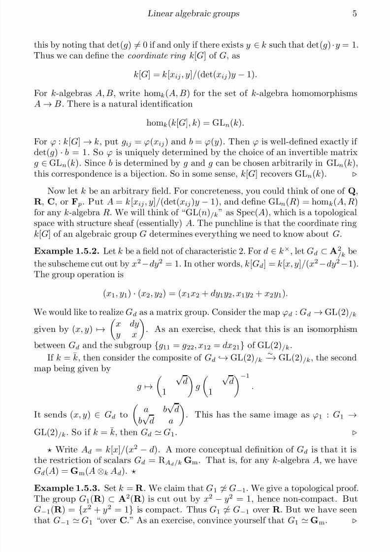
Example 1.5.2. Let k be a field not of characteristic 2. For d ∈ k×, let Gd ⊂ A2/k be
the subscheme cut out by x2−dy2 = 1. In other words, k[Gd] = k[x, y]/(x2−dy2 −1).The group operation is
(x1, y1) · (x2, y2) = (x1x2 + dy1y2, x1y2 + x2y1).
We would like to realize Gd as a matrix group. Consider the map ϕd : Gd → GL(2)/k
given by (x, y) →
x dyy x
. As an exercise, check that this is an isomorphism
between Gd and the subgroup {g11 = g22, x12 = dx21} of GL(2)/k.
If k = k, then consider the composite of Gd → GL(2)/k∼−→ GL(2)/k, the second
map being given by
g → √
d1 g
√ d
1 −1
.
It sends (x, y) ∈ Gd to
a b
√ d
b√
d a
. This has the same image as ϕ1 : G1 →
GL(2)/k. So if k = k, then Gd G1.
Write Ad = k[x]/(x2 − d). A more conceptual definition of Gd is that it isthe restriction of scalars Gd = RAd/k Gm. That is, for any k-algebra A, we haveGd(A) = Gm(A ⊗k Ad).
Example 1.5.3. Set k = R. We claim that G1 G−1. We give a topological proof.The group G1(R) ⊂ A2(R) is cut out by x2 − y2 = 1, hence non-compact. ButG−1(R) = {x2 + y2 = 1} is compact. Thus G1 G−1 over R. But we have seenthat G−1 G1 “over C.” As an exercise, convince yourself that G1 Gm.
7/18/2019 Linear algebraic groups and their Lie algebras
http://slidepdf.com/reader/full/linear-algebraic-groups-and-their-lie-algebras 6/81
Linear algebraic groups 6
It turns out that “twists of Gm over k up to isomorphism” are in bijectivecorrespondence with k×/2, via the correspondence d → Gd.
This is easy to see. The k-forms of Gm is in natural bijection with H1(k, Aut Gm) =H1(k, Z/2). Kummer theory tells us that H1(k, Z/2) = k×/2.
1.6 Structure theory for linear algebraic groups
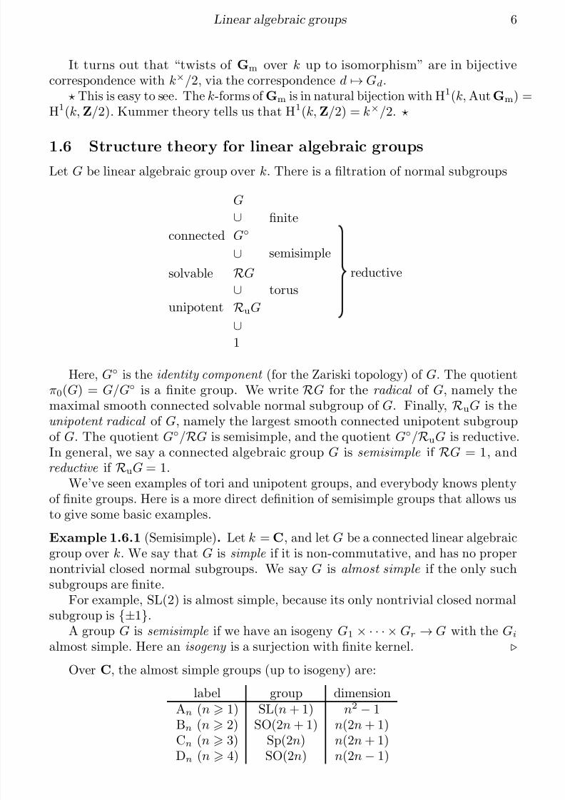
Let G be linear algebraic group over k. There is a filtration of normal subgroups
G
∪ finite
connected G◦
∪ semisimple
solvable RG∪ torus
unipotent RuG
∪1
reductive
Here, G◦ is the identity component (for the Zariski topology) of G. The quotientπ0(G) = G/G◦ is a finite group. We write RG for the radical of G, namely themaximal smooth connected solvable normal subgroup of G. Finally,
RuG is the
unipotent radical of G, namely the largest smooth connected unipotent subgroupof G. The quotient G◦/RG is semisimple, and the quotient G◦/RuG is reductive.In general, we say a connected algebraic group G is semisimple if RG = 1, andreductive if RuG = 1.
We’ve seen examples of tori and unipotent groups, and everybody knows plentyof finite groups. Here is a more direct definition of semisimple groups that allows usto give some basic examples.
Example 1.6.1 (Semisimple). Let k = C, and let G be a connected linear algebraicgroup over k. We say that G is simple if it is non-commutative, and has no propernontrivial closed normal subgroups. We say G is almost simple if the only suchsubgroups are finite.
For example, SL(2) is almost simple, because its only nontrivial closed normalsubgroup is {±1}.
A group G is semisimple if we have an isogeny G1 × · · · × Gr → G with the Gi
almost simple. Here an isogeny is a surjection with finite kernel.
Over C, the almost simple groups (up to isogeny) are:
label group dimensionAn (n 1) SL(n + 1) n2 − 1Bn (n 2) SO(2n + 1) n(2n + 1)Cn (n 3) Sp(2n) n(2n + 1)Dn (n 4) SO(2n) n(2n − 1)
7/18/2019 Linear algebraic groups and their Lie algebras
http://slidepdf.com/reader/full/linear-algebraic-groups-and-their-lie-algebras 7/81
Linear algebraic groups 7
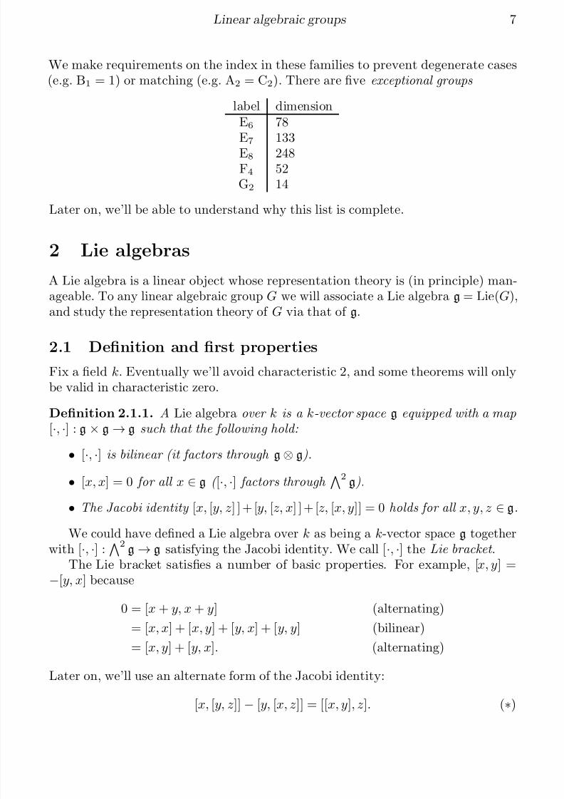
We make requirements on the index in these families to prevent degenerate cases(e.g. B1 = 1) or matching (e.g. A2 = C2). There are five exceptional groups
label dimensionE6 78
E7 133E8 248F4 52G2 14
Later on, we’ll be able to understand why this list is complete.
2 Lie algebras
A Lie algebra is a linear object whose representation theory is (in principle) man-ageable. To any linear algebraic group G we will associate a Lie algebra g = Lie(G),and study the representation theory of G via that of g.
2.1 Definition and first properties
Fix a field k. Eventually we’ll avoid characteristic 2, and some theorems will onlybe valid in characteristic zero.
Definition 2.1.1. A Lie algebra over k is a k-vector space g equipped with a map[·, ·] : g × g → g such that the following hold:
• [·, ·] is bilinear (it factors through g ⊗ g).
• [x, x] = 0 for all x ∈ g ( [·, ·] factors through 2
g).
• The Jacobi identity [x, [y, z] ] + [y, [z, x] ] + [z, [x, y]] = 0 holds for all x, y, z ∈ g.
We could have defined a Lie algebra over k as being a k-vector space g togetherwith [
·,
·] : 2
g
→ g satisfying the Jacobi identity. We call [
·,
·] the Lie bracket .
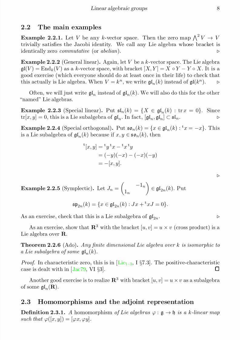
The Lie bracket satisfies a number of basic properties. For example, [x, y] =−[y, x] because
0 = [x + y, x + y] (alternating)
= [x, x] + [x, y] + [y, x] + [y, y] (bilinear)
= [x, y] + [y, x]. (alternating)
Later on, we’ll use an alternate form of the Jacobi identity:
[x, [y, z]] − [y, [x, z]] = [[x, y], z]. (∗)
7/18/2019 Linear algebraic groups and their Lie algebras
http://slidepdf.com/reader/full/linear-algebraic-groups-and-their-lie-algebras 8/81
Linear algebraic groups 8
2.2 The main examples
Example 2.2.1. Let V be any k-vector space. Then the zero map 2 V → V
trivially satisfies the Jacobi identity. We call any Lie algebra whose bracket isidentically zero commutative (or abelian ).
Example 2.2.2 (General linear). Again, let V be a k-vector space. The Lie algebragl(V ) = Endk(V ) as a k-vector space, with bracket [X, Y ] = X ◦ Y − Y ◦ X . It is agood exercise (which everyone should do at least once in their life) to check thatthis actually is Lie algebra. When V = kn, we write gln(k) instead of gl(kn).
Often, we will just write gln instead of gln(k). We will also do this for the other“named” Lie algebras.
Example 2.2.3 (Special linear). Put sln(k) = {X ∈ gln(k) : tr x = 0}. Since
tr[x, y] = 0, this is a Lie subalgebra of gln. In fact, [gln, gln] ⊂ sln. Example 2.2.4 (Special orthogonal). Put son(k) = {x ∈ gln(k) : tx = −x}. Thisis a Lie subalgebra of gln(k) because if x, y ∈ son(k), then
t[x, y] = ty tx − tx ty
= (−y)(−x) − (−x)(−y)
= −[x, y].
Example 2.2.5 (Symplectic). Let J n =
−1n1n
∈ gl2n(k). Put
sp2n(k) = {x ∈ gl2n(k) : J x + txJ = 0}.
As an exercise, check that this is a Lie subalgebra of gl2n.
As an exercise, show that R3 with the bracket [u, v] = u × v (cross product) is aLie algebra over R.
Theorem 2.2.6 (Ado). Any finite dimensional Lie algebra over k is isomorphic toa Lie subalgebra of some gln(k).
Proof. In characteristic zero, this is in [Lie1–3, I §7.3]. The positive-characteristiccase is dealt with in [Jac79, VI §3].
Another good exercise is to realize R3 with bracket [u, v] = u × v as a subalgebraof some gln(R).
2.3 Homomorphisms and the adjoint representation
Definition 2.3.1. A homomorphism of Lie algebras ϕ : g → h is a k-linear mapsuch that ϕ([x, y]) = [ϕx, ϕy].
7/18/2019 Linear algebraic groups and their Lie algebras
http://slidepdf.com/reader/full/linear-algebraic-groups-and-their-lie-algebras 9/81
Linear algebraic groups 9
If ϕ : g → h is a homomorphism of Lie algebras, then a = ker(ϕ) is a Liesubalgebra of g. This is easy:
ϕ[x, y] = [ϕ(x), ϕ(y)]
= [0, 0]
= 0.
Definition 2.3.2. A Lie subalgebra a of g is an ideal if [a, g] ⊂ a, i.e. [a, x] ∈ a for all a ∈ a, x ∈ g.
Equivalently, a ⊂ g is an ideal if [g, a] ⊂ a. If a ⊂ g is an ideal, we define thequotient algebra g/a to be g/a as a vector space, with bracket induced by that of g.So
[x + a, y + a] = [x, y] + a.
Let’s check that this makes sense. If a1, a2 ∈ a, then
[x + a1, x + a2] = [x, y] + [x, a2] + [a1, y] + [a1, a2]
≡ [x, y] (mod a).
If ϕ : g → h is a Lie homomorphism, then we get an induced isomorphismg/ ker(ϕ)
∼−→ im(ϕ) ⊂ h.
Example 2.3.3. Give k the trivial Lie bracket. Then tr : gln(k) → k is a ahomomorphism. Indeed,
tr[x, y] = tr(xy) − tr(yx) = 0.
We could have defined sln(k) = ker(tr); this is an ideal in gln, and gln(k)/ sln(k) ∼−→
k.
Definition 2.3.4. Let g be a Lie algebra over k. The adjoint representation of g is the map ad : g → gl(g) defined by ad(x)(y) = [x, y] for x, y ∈ g.
It is easy to check that ad : g → gl(g) is k-linear, that is ad(cx) = c ad(x) andad(x + y) = ad(x) + ad(y). It is bit less obvious how the adjoint action behaves withrespect to the Lie bracket. We compute
ad([x, y])(z) = [[x, y], z]
=(∗) [x, [y, z]] − [y, [x, z]]
= (ad(x)ad(y))(z) − (ad(y)ad(x))(z).
Thus ad[x, y] = [ad(x), ad(y)] and we have shown that ad : g → gl(g) is a homo-morphism of Lie algebras. If n = dimk(g) < ∞, then ad : g → gl(g) gln(k) isan interesting finite-dimensional representation of g. If dim(g) > 1, it cannot be
surjective, and there are easy ways for it to fail to be injective.
Definition 2.3.5. Let g be a Lie algebra over k. The center of g is
Z(g) = {x ∈ g : [x, y] = 0 for all y ∈ g}.
7/18/2019 Linear algebraic groups and their Lie algebras
http://slidepdf.com/reader/full/linear-algebraic-groups-and-their-lie-algebras 10/81
Linear algebraic groups 10
Note that Z(g) = ker(ad). There is a natural injection g/ Z(g) → gl(g).
Definition 2.3.6. A Lie algebra g is simple if it is non-commutative, and has noideals except 0 and g.
Just as with simple algebraic groups, there is a classification theorem for simpleLie algebras. Even better, since Lie algebras are more “rigid” than algebraic groups,we don’t have to worry about isogeny.
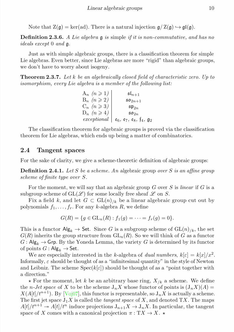
Theorem 2.3.7. Let k be an algebraically closed field of characteristic zero. Up toisomorphism, every Lie algebra is a member of the following list:
An ( n 1) sln+1
Bn ( n 2) so2n+1
Cn ( n 3) sp2n
Dn ( n 4) so2n
exceptional e6, e7, e8, f4, g2
The classification theorem for algebraic groups is proved via the classificationtheorem for Lie algebras, which ends up being a matter of combinatorics.
2.4 Tangent spaces
For the sake of clarity, we give a scheme-theoretic definition of algebraic groups:
Definition 2.4.1. Let S be a scheme. An algebraic group over S is an affine groupscheme of finite type over S .
For the moment, we will say that an algebraic group G over S is linear if G is asubgroup scheme of GL(L ) for some locally free sheaf L on S .
Fix a field k, and let G ⊂ GL(n)/k be a linear algebraic group cut out bypolynomials f 1, . . . , f r. For any k-algebra R, we define
G(R) = {g ∈ GLn(R) : f 1(g) = · · · = f r(g) = 0}.
This is a functor Algk →
Set. Since G is a subgroup scheme of GL(n)/k, the setG(R) inherits the group structure from GLn(R). So we will think of G as a functorG : Algk → Grp. By the Yoneda Lemma, the variety G is determined by its functorof points G : Algk → Set.
We are especially interested in the k-algebra of dual numbers , k[ε] = k[x]/x2.Informally, ε should be thought of as a “infinitesimal quantity” in the style of Newtonand Leibniz. The scheme Spec(k[ε]) should be thought of as a “point together witha direction.”
For the moment, let k be an arbitrary base ring, X /k a scheme. We definethe n-Jet space of X to be the scheme JnX whose functor of points is (JnX )(A) =X (A[t]/tn+1). By [Voj07], this functor is representable, so JnX is actually a scheme.The first jet space J1X is called the tangent space of X , and denoted TX . The mapsA[t]/tn+1 A[t]/tn induce projections Jn+1X → JnX . In particular, the tangentspace of X comes with a canonical projection π : TX → X .
7/18/2019 Linear algebraic groups and their Lie algebras
http://slidepdf.com/reader/full/linear-algebraic-groups-and-their-lie-algebras 11/81
Linear algebraic groups 11
Consider G(k[ε]). As a set, this consists of invertible n × n matrices with entriesin k[ε] on which the f i vanish. The map ε → 0 from k[ε] → k induces a grouphomomorphism π : G(k[ε]) → G(k). We will consider this map as the “tangentspace” of G(k). For each g ∈ G(k), the fiber π−1(g) is the “tangent space of G atg.”
Note that
π−1(g) = {g + εv : v ∈ Mn(k) : f i(g + εv) = 0 for all i}.
For each s, the polynomial f s has a Taylor series expansion
f s(xij) = f s(g) +i,j
∂f s∂xi,j
(g)(xi,j − gi,j).
Since f s(g) = 0, we get f s(g + εv) = εi,j∂f s∂xi,j (g)vi,j . It follows that
π−1(g) =
g + εv : v ∈ Mn(k) :i,j
∂f s∂xij
(g)vij = 0 for all 1 s r
.
We will be especially interested in g = π−1(1). We will turn this into a Lie algebrausing the group structure on G.
From the scheme-theoretic perspective, the identity element 1 ∈ G(k) comes
from a section e : Spec(k) → G of the structure G → Spec(k). The scheme-theoretic Lie algebra of G is the fiber product
g = e∗1 = T(G) ×G Spec(k).
By definition, g(A) = ker(G(A[ε]) → G(A)) for any k-algebra A. Just as withalgebraic groups, we will write g/k for g thought of as a group scheme over k, and
just g for g(k).
2.5 Functors of pointsRecall that schemes can be thought of as functors Algk → Set. For example, affinen-space is the functor An(A) = An. In fact, this is an algebraic group, the operationcoming from addition on A. Moreover, An is representable in the sense that
An(A) = homk(k[x1, . . . , xn], A),
via (a1, . . . , an) → (xi → ai). Similarly, SL(n)/k sends a k-algebra A to SLn(A). Itis represented by the ring k[xij ]/(det(x)
−1). In general, we take some polynomials
f 1, . . . , f r ∈ k[x1, . . . , xn], and consider the subscheme X = V (f 1, . . . , f r) ⊂ An
which represents the functor
X (A) = {a ∈ An : f 1(a) = · · · = f r(a) = 0}.
7/18/2019 Linear algebraic groups and their Lie algebras
http://slidepdf.com/reader/full/linear-algebraic-groups-and-their-lie-algebras 12/81
Linear algebraic groups 12
This has coordinate ring k[x1, . . . , xn]/(f 1, . . . , f r). Note that any finitely generatedk-algebras is of this form. In other words, all affine schemes of finite type over k aresubschemes of some affine space.
Clasically, one gives X (k) the Zariski topology . If f ∈ k[X ] = A1(X ), we get (bydefinition) a function f : X (k)
→ k. We define open subsets of X (k) to be those of
the form {x ∈ X (k) : f (x) = 0}. More scheme-theoretically, we say that an open subscheme of X is the complement of any V (f ) for f ∈ k[X ].
We can think of the Zariski topology as giving a Grothendieck topology on thecategory of affine schemes over k. It is subcanonical, i.e. all representable functorsare sheaves. So if we formally put Aff k = (Algk)◦, then the category of schemes overk embeds into Shzar(Aff k). When working with algebraic groups, often it is betterwith the etale or fppf topologies. In particular, we will think of quotients as livingin Shfppf (Aff k).
Definition 2.5.1. Let k be a feld. A variety over k is a reduced separated scheme of finite type over k.
In particular, an affine variety is determined by a reduced k-algebra. We candirectly associate a “geometric object” to a k-algebra A, namely its spectrum Spec(A) = {p ⊂ A prime ideal}. Finally, we note that if X = Spec(A) is of finitetype over k and if k = k, then X (k) = homk(A, k) is the set of maximal ideas in A.
2.6 Affine group schemes and Hopf algebras
An affine group G/k will give us a functor G : Algk → Grp. As such, it should havemorphisms
m : G × G → G “multiplication”
e : 1 = Spec(k) → G “identity”
i : G → G “inverse”
These correspond to ring homomorphisms
∆ : A → A ⊗k A “comultiplication”ε : A → k “counit”
σ : A → A “coinverse”
Obviously the maps on groups satisfy some axioms like associativity etc. These canbe phrased by the commutativity of diagrams like
G × G × G G × G
G × G G.
id×m
m×id m
m
Most sources do not give all these diagrams explicitly. One that does is the book[Wat79].
7/18/2019 Linear algebraic groups and their Lie algebras
http://slidepdf.com/reader/full/linear-algebraic-groups-and-their-lie-algebras 13/81
Linear algebraic groups 13
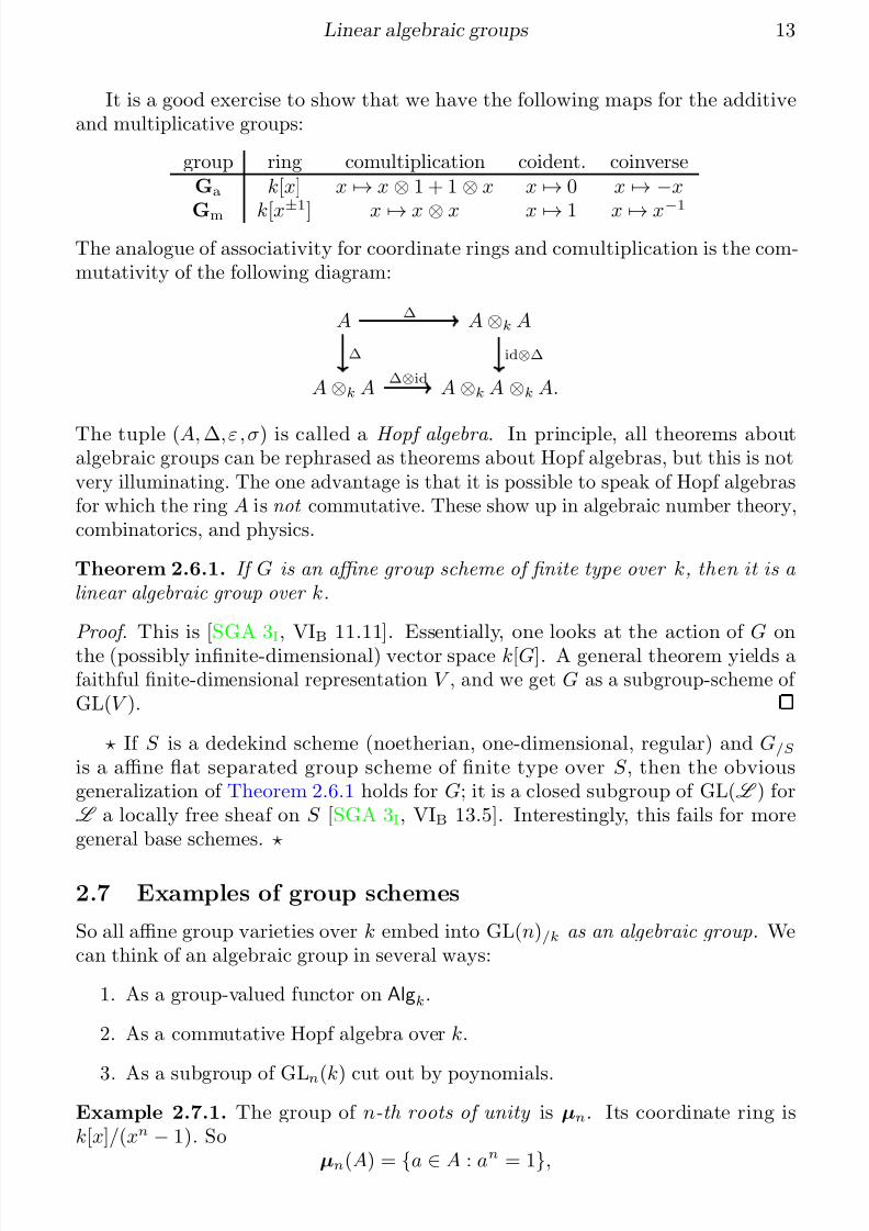
It is a good exercise to show that we have the following maps for the additiveand multiplicative groups:
group ring comultiplication coident. coinverseGa k[x] x → x ⊗ 1 + 1 ⊗ x x → 0 x → −x
Gm k[x±1
] x → x ⊗ x x → 1 x → x−1
The analogue of associativity for coordinate rings and comultiplication is the com-mutativity of the following diagram:
A A ⊗k A
A ⊗k A A ⊗k A ⊗k A.
∆
∆ id⊗∆
∆⊗id
The tuple (A, ∆, ε , σ) is called a Hopf algebra . In principle, all theorems aboutalgebraic groups can be rephrased as theorems about Hopf algebras, but this is notvery illuminating. The one advantage is that it is possible to speak of Hopf algebrasfor which the ring A is not commutative. These show up in algebraic number theory,combinatorics, and physics.
Theorem 2.6.1. If G is an affine group scheme of finite type over k, then it is a linear algebraic group over k.
Proof. This is [SGA 3I, VIB 11.11]. Essentially, one looks at the action of G onthe (possibly infinite-dimensional) vector space k[G]. A general theorem yields afaithful finite-dimensional representation V , and we get G as a subgroup-scheme of GL(V ).
If S is a dedekind scheme (noetherian, one-dimensional, regular) and G/S
is a affine flat separated group scheme of finite type over S , then the obviousgeneralization of Theorem 2.6.1 holds for G; it is a closed subgroup of GL(L ) forL a locally free sheaf on S [SGA 3I, VIB 13.5]. Interestingly, this fails for moregeneral base schemes.
2.7 Examples of group schemes
So all affine group varieties over k embed into GL(n)/k as an algebraic group. Wecan think of an algebraic group in several ways:
1. As a group-valued functor on Algk.
2. As a commutative Hopf algebra over k.
3. As a subgroup of GLn(k) cut out by poynomials.Example 2.7.1. The group of n-th roots of unity is µn. Its coordinate ring isk[x]/(xn − 1). So
µn(A) = {a ∈ A : an = 1},
7/18/2019 Linear algebraic groups and their Lie algebras
http://slidepdf.com/reader/full/linear-algebraic-groups-and-their-lie-algebras 14/81
Linear algebraic groups 14
with the group operation coming from multiplication in A. Note that µn ⊂ Gm.If the base field k has characteristic p n, then µn(k) is a cyclic group of order n.However, if n = p, then x p − 1 = (x − 1) p. So the coordinate ring k[x]/((x − 1) p)is non-reduced. This is our first example of a group scheme that is not a groupvariety. One realization of this is that µ p(F p) = 1. These problems can only occur
in characteristic p > 0. If G is a group scheme over a characteristic zero field, thenG is automatically reduced.
Let φ : Gm → Gm be the homomorphism x → x p. Note that ker(φ) = µ p. OnF p-points, this map is an isomorphism, but φ is not an isomorphism of algebraicgroups.
Let G/k be a linear algebraic group. Recall that we defined the Lie algebra g = Lie(G) of G to be the functor on k-algebras given by
g(A) = ker G(A[ε]/ε2)
→ G(A) .
In subsection 2.4, we saw that if G ⊂ GL(n)/k is cut out by f 1, . . . , f r, then thek-valued points could be computed as
g =
X ∈ Mn(k) :i,j
∂f α∂xij
(1n) · X ij = 0
.
Example 2.7.2 (Special linear). Consider SL(n)/k ⊂ GL(n)/k, cut out by det = 1.Its Lie algebra sln = Lie( sln) is
sln = {1 + xε : x ∈ Mn(k) and det(1 + xε) = 1} .
The expansion of determinant is det(1 + xε) = 1 + tr(x)ε + O(ε2). Thus
sln = {x ∈ Mn : tr(x) = 0} .
As a functor on k-algebras, sln(A) = {x ∈ Mn(A) : tr x = 0}.
Example 2.7.3 (Orthogonal). Recall that O(n) ⊂ GL(n) is cut out by g tg = 1. So
Lie(On) = {
1 + xε : (1 + xε) t(1 + xε) = 1}
= {1 + Xε : x + tX = 0} {X ∈ Mn : tx = −x}= son.
If the characteristic of the base field is not 2, then dim( son) = n(n − 1)/2.
2.8 Lie algebra of an algebraic group
Fix a field k. Let G/k be a linear algebraic group. For any k-algebra A, writeA[ε] = k[t]/t2. Then A → G(A[ε]) is a new group functor, and we can define theLie algebra of G to be
Lie(G)(A) = ker(G(A[ε]) → G(A)) .
7/18/2019 Linear algebraic groups and their Lie algebras
http://slidepdf.com/reader/full/linear-algebraic-groups-and-their-lie-algebras 15/81
Linear algebraic groups 15
A priori, this is a group functor. Often, we will write g = Lie(G) to mean Lie(G)(k).If G ⊂ GL(n) is cut out by f 1, . . . , f r, then
g = {1 + εx : x ∈ Mn(k) and f α(1 + εx) = 0 for all α} .
The group operation is addition on x, i.e. (1 + εx)(1 + εy) = 1 + ε(x + y). Thus g isa k-vector space.
This section will contain many “high-level” interludes on the functorial definitionof Lie(G). They are all strongly influenced by the exposition in [SGA 3I, II §3–4].Let O : Algk → Algk be the functor A → A. Note that O is represented by k[t].Thus A1
/k has the structure not only of a group scheme, but of a k-ring scheme,
or (k, k)-biring in the sense of [BW05]. We define an O -module to be a functorV : Algk → Set such that for each A, the set V (A) is given an O (A) = A-modulestructure in a functorial way.
If S : Algk →
Set is a functor, we will write SchS
for the category of representablefunctors X : Algk → Set together with a morphism X → S . A morphism (X →S ) → (Y → S ) in SchS is a morphism of functors X → Y making the followingdiagram commute:
X Y
S.
There is an easy generalization of O to a ring object O ∈ SchS . It sends a scheme
X to the ring H
0
(X,O X) of regular functions on X .For a scheme X , the first jet space J1X is naturally an O -module in SchX . We
could be fancy and say that for any ring A, A[ε] is naturally an abelian group object
in AlgA/A, or we could define the O -module structure on J1X π−→ X directly. For
ϕ : Spec(A) → X , we need to give
(J1X )/X(A) = {f ∈ (J1X )(A) : π ◦ f = ϕ}the structure of an A-module. Given a ∈ A, define σa : A[ε] → A[ε] by ε → aε. Thisis a ring homomorphism, so it induces σa : J1X (A) → J1X (A). The restriction of
this map to (J1X )/X(A) is the desired action of A. See [SGA 3I, II 3.4.1] for a morecareful proof that this gives (J1X )/X the structure of an O -module in SchX .
The point of all this is that if M is an O -module in SchY and f : X → Y is amorphism of schemes, then f ∗M , defined by
(f ∗M )(Spec(A) p−→ X ) = M (Spec(A)
p−→ X f −→ Y )
is naturally an O -module in SchX . So if G is an algebraic group, J1X is naturallyan O -module in SchG, and the morphism e : 1 → G gives g = e∗J1G the structureof an O -module in Schk.
Example 2.8.1 (Symplectic). Let J = −1n
1n
. Recall that
Sp2n(A) =
g ∈ GL2n(A) : tgJ g = J
.
7/18/2019 Linear algebraic groups and their Lie algebras
http://slidepdf.com/reader/full/linear-algebraic-groups-and-their-lie-algebras 16/81
Linear algebraic groups 16
Let’s compute the Lie algebra of Sp2n. For X ∈ M2n(A), we have
t(1 + εx)J (1 + εx) = (1 + ε tx)J (1 + εx)
= J + ε(txJ + Jx).
So sp2n(A) {x ∈ M2n(A) : txJ + Jx = 0}.
Algebraic groups can be highly non-abelian, and so far all we’ve done is giveg = Lie(G) the structure of a vector space. We’d like to give g the structure of a Liealgebra.
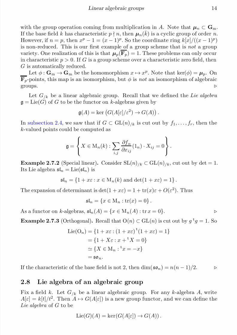
Let f : G → H be a homomorphism of algebraic groups. Then f : G(A) → H (A)is a homomorphism for all k-algebras A. A morphism f : G → H correspondsby the Yoneda Lemma to a unique element ϕ ∈ homk(k[H ], k[G]). For all A,the induced map G(A) → H (A) is defined by ψ → ψ ◦ ϕ via the identificationsG(A) = hom(k[G], A) and H (A) = hom(k[H ], A).
Example 2.8.2. Recall that Gm(A) = A× = hom(k[x±1], A). All homomorphismsf : Gm → Gm come from x → xn for some n ∈ Z. On functors of points, this isa → an for a ∈ A×.
As before, let f : G → H be a morphism of algebraic groups. Let g = Lie(G),h = Lie(G). There is an induced map Lie(f ) : g → h. On functors of points, it isinduced by the inclusions g ⊂ J1G, h ⊂ J1H and the fact that f : J1G → J1H is agroup homomorphism. That is, for each k-algebra A, f ∗ : g(A) → h(A) is induced
by the commutative diagram
G(A[ε]) H (A[ε])
g(A) h(A).
f
f ∗
In particular, a representation ρ : G → GL(n) induces a map on Lie algebrasg → gln.
The natural way of stating the above is that Lie is a functor from groupschemes over k to O -modules in Schk. What’s more, if G is a group scheme andg = Lie(G), then by [SGA 3I, II 3.3], there is a natural isomorphism of A-modulesg(k) ⊗k A
∼−→ g(A). So the functor g is actually determined by the vector space g(k).This justifies our passing between g and g(k).
Let’s construct the Lie bracket on the Lie algebra of an algebraic group. Recallthat for a Lie algebra g, we defined a map ad : g → gl(g) = Endk(g) by ad(x)(y) =[x, y]. The bracket on g is clearly determined by the adjoint map.
For g = Lie(G), we’ll define the adjoint map directly, then use this to give g thestructure of a Lie algebra. For any g
∈ G(A), we have an action ad(g) : GA
→ GA
given by x → gxg−1 for any B ∈ AlgA. So we have a homomorphism of groupfunctors ad : G → Aut(G). In particular, G(k) acts on G by k-automorphisms.
The general philosophy, due to Grothendieck and worked out carefully in SGA,is that “everything is a functor.” That is, we think of every object as living in the
7/18/2019 Linear algebraic groups and their Lie algebras
http://slidepdf.com/reader/full/linear-algebraic-groups-and-their-lie-algebras 17/81
Linear algebraic groups 17
category of functors Algk → Set. For example, if X and Y are schemes over k, thenhom(X, Y ) is the functor whose
hom(X, Y )(A) = homSchA(X A, Y A).
We recover the usual hom-set as hom(X, Y )(k). Similarly, we define Aut(G)(A) =AutGrpA(GA). These functors are not usually representable, but they are sheaves forall the reasonable Grothendieck topologies on Schk. See [SGA 3I, I §1–3, II §1] for acareful exposition along these lines.
By functoriality, there is a natural homomorphism Aut(G) → Aut(g). Composingthis with the map ad : G → Aut(G) gives a map ad : G → Aut(g). Explicitly, themap ad : G(A) → Aut(g)(A) = Aut(gA) sends g to the automorphism x → gxg−1
for any x ∈ G(B[ε]), B ∈ AlgA. It is easy to see that this action respects O -module structure on g, so we in fact have a representation ad : G → GL(g). Since
g(A) = g(k)⊗k A, we can think of g as an honest k-vector space and define GL(g) asthe functor A → AutA(g⊗k A). In either case, we have a morphism ad : G → GL(g)of linear algebraic groups.
Apply Lie(−) to the adjoint representation ad : G → GL(g). We get a mapad : g → Lie(GL(g)) = gl(g). We claim that g together with [x, y] = ad(x)(y) is aLie algebra.
Example 2.8.3. Let G = GL(n). We wish to verify that our functorial definition of ad : gln → gl(gln) agrees with the elementary definition ad(x)(y) = [x, y]. Start withthe action of GL(n) on gl
n. For any k-algebra A, this is the action by conjugation
of GLn(A) ⊂ GLn(A[ε]) on gln(A) = ker(GLn(A[ε]) → GLn(A)). This is because
g · (1 + εx)(g−1) = 1 + ε ad(g)(x).
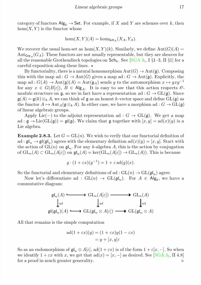
So the functorial and elementary definitions of ad : GL(n) → GL(gln) agree.Now let’s differentiate ad : GL(n) → GL(gln). For A ∈ Algk, we have a
commutative diagram:
gln(A) GLn(A[ε]) GLn(A)
gl(gln)(A) GL(gln ⊗ A[ε]) GL(gln ⊗ A)
ad ad ad
All that remains is the simple computation
ad(1 + εx)(y) = (1 + εx)y(1 − εx)
= y + [x, y]ε
So as an endomorphism of gln ⊗ A[ε], ad(1 + εx) is of the form 1 + ε[x, −]. So whenwe identify 1 + εx with x, we get that ad(x) = [x, −] as desired. See [SGA 3I, II 4.8]for a proof in much greater generality.
7/18/2019 Linear algebraic groups and their Lie algebras
http://slidepdf.com/reader/full/linear-algebraic-groups-and-their-lie-algebras 18/81
Linear algebraic groups 18
This example yields the general fact that Lie(G) is a Lie algebra. Choose anembedding G → GL(n). By construction, the Lie functor is limit-preserving, sog → gln. The bracket on g (as a subspace of gln is induced by the bracket ongln. We have seen that the functorial definition of the bracket on gln matches theelementary definition, so gln is a Lie algebra and g is a Lie subalgebras of gln.
Does Lie(G) determine G? The answer is an easy no! For example, SO(n) andO(n) both have Lie algebra son. Also SL(n) and PSL(n) both have Lie algebra sln.There is are the easy example Lie(Ga) = Lie(Gm) = gl1. Finally, Lie(G) = Lie(G◦),so Lie(G) does not depend on the group π0(G) = G/G◦ of connected componentsof G. However, given a semisimple Lie algebra g, there is a unique split connected,simply-connected semisimple algebraic group G with Lie(G) = g.
Example 2.8.4. Let’s go over the Lie bracket on GL(n) in a more elementarymanner. We have
gln = ker (GLn(k[ε]) → GLn(k)) = {1 + εx : x ∈ Mn(k)} ∼−→ Mn(k).
We’ll write elements of Mn(k[ε]) as x + yε; these should be thought of as a “point” xtogether with an “infinitesimal direction” y. The adjoint map is the homomorphismad : GL(n) → GL(gln), defined on A-points as the map GLn(A) → GL(gln(A))given by ad(g)(x) = gxg−1. So for A = k[ε], the group GLn(k[ε]) acts on Mn(k[ε])by conjugation. Take any 1 + εb ∈ GLn(k[ε]), and any x + εy ∈ Mn(k[ε]). Wecompute:
(1 + εb)(x + εy)(1−
εb)−1 = (x + εy + εbx)(1−
εb)
= x + εy + ε(bx − xb)
= x + εy + ε[b, x]
= (1 + ε[b, −])(x + εy).
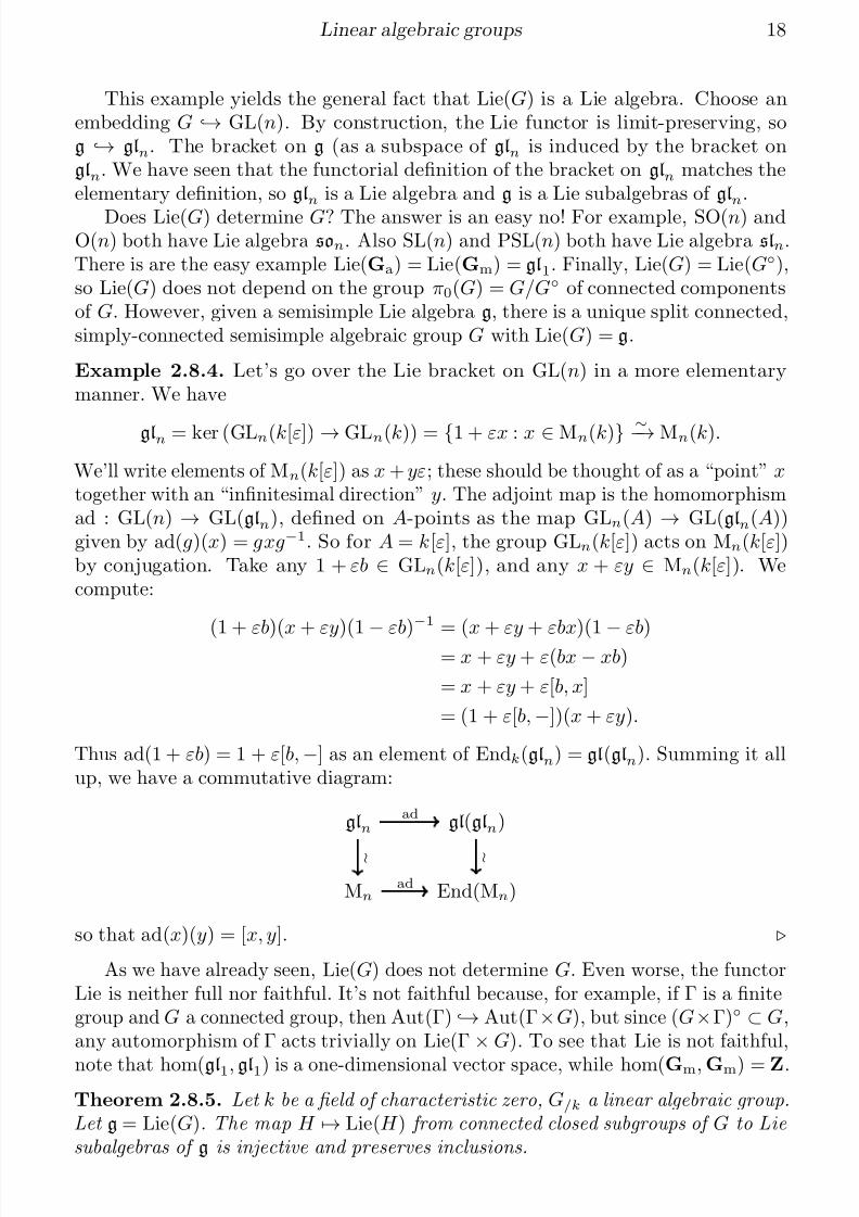
Thus ad(1 + εb) = 1 + ε[b, −] as an element of Endk(gln) = gl(gln). Summing it allup, we have a commutative diagram:
gln gl(gln)
Mn End(Mn)
ad
ad
so that ad(x)(y) = [x, y].
As we have already seen, Lie(G) does not determine G. Even worse, the functorLie is neither full nor faithful. It’s not faithful because, for example, if Γ is a finitegroup and G a connected group, then Aut(Γ) → Aut(Γ×G), but since (G×Γ)◦ ⊂ G,any automorphism of Γ acts trivially on Lie(Γ × G). To see that Lie is not faithful,
note that hom(gl1, gl1) is a one-dimensional vector space, while hom(Gm, Gm) = Z.Theorem 2.8.5. Let k be a field of characteristic zero, G/k a linear algebraic group.Let g = Lie(G). The map H → Lie(H ) from connected closed subgroups of G to Lie subalgebras of g is injective and preserves inclusions.
7/18/2019 Linear algebraic groups and their Lie algebras
http://slidepdf.com/reader/full/linear-algebraic-groups-and-their-lie-algebras 19/81
Linear algebraic groups 19
Proof. If H 1 ⊂ H 2, use the functoriality of forming Lie algebras to see that Lie(H 1) ⊂Lie(H 2) as subalgebras of g. The nontrivial part is to show that Lie(H ), as asubalgebra of g, determines H . Let H 1, H 2 be be two closed connected subgroups of G such that h = Lie(H 1) = Lie(H 2). Then H 3 = (H 1 ∩ H 2)◦ is a closed connectedsubgroup of G. Since fiber products are computed pointwise and the Lie functor
is exact, we have Lie(H 3) = h. By Theorem 2.8.7, the H i are all smooth, sodim(H i) = dim h. But the only way H 3 ⊂ H 1 can both be smooth and irreduciblewith the same dimension is for H 1 = H 3. Similarly H 2 = H 3, so H 1 = H 2.
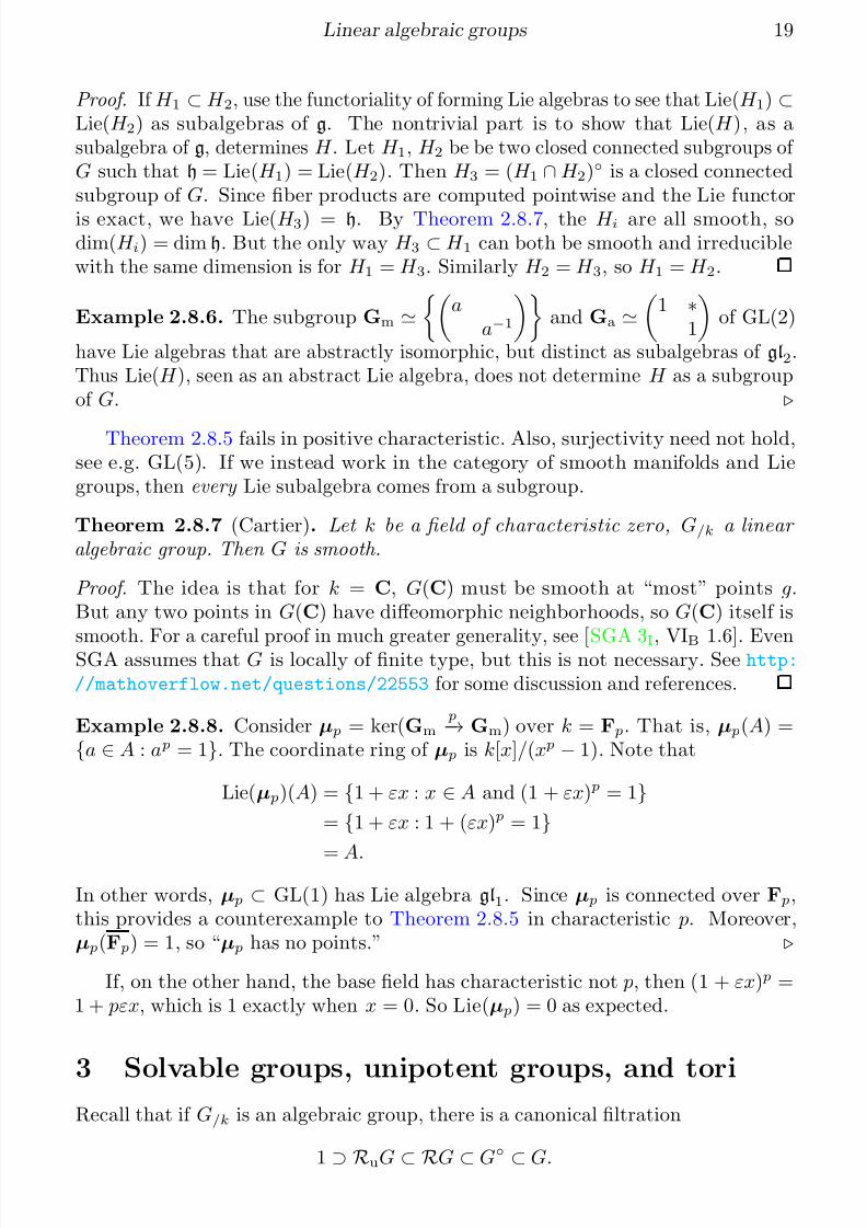
Example 2.8.6. The subgroup Gm
aa−1
and Ga
1 ∗
1
of GL(2)
have Lie algebras that are abstractly isomorphic, but distinct as subalgebras of gl2.Thus Lie(H ), seen as an abstract Lie algebra, does not determine H as a subgroupof G.
Theorem 2.8.5 fails in positive characteristic. Also, surjectivity need not hold,see e.g. GL(5). If we instead work in the category of smooth manifolds and Liegroups, then every Lie subalgebra comes from a subgroup.
Theorem 2.8.7 (Cartier). Let k be a field of characteristic zero, G/k a linear algebraic group. Then G is smooth.
Proof. The idea is that for k = C, G(C) must be smooth at “most” points g.But any two points in G(C) have diffeomorphic neighborhoods, so G(C) itself is
smooth. For a careful proof in much greater generality, see [SGA 3I, VIB 1.6]. EvenSGA assumes that G is locally of finite type, but this is not necessary. See http://mathoverflow.net/questions/22553 for some discussion and references.
Example 2.8.8. Consider µ p = ker(Gm p−→ Gm) over k = F p. That is, µ p(A) =
{a ∈ A : a p = 1}. The coordinate ring of µ p is k[x]/(x p − 1). Note that
Lie(µ p)(A) = {1 + εx : x ∈ A and (1 + εx) p = 1}= {1 + εx : 1 + (εx) p = 1}
= A.
In other words, µ p ⊂ GL(1) has Lie algebra gl1. Since µ p is connected over F p,this provides a counterexample to Theorem 2.8.5 in characteristic p. Moreover,µ p(F p) = 1, so “µ p has no points.”
If, on the other hand, the base field has characteristic not p, then (1 + εx) p =1 + pεx, which is 1 exactly when x = 0. So Lie(µ p) = 0 as expected.
3 Solvable groups, unipotent groups, and toriRecall that if G/k is an algebraic group, there is a canonical filtration
1 ⊃ RuG ⊂ RG ⊂ G◦ ⊂ G.
7/18/2019 Linear algebraic groups and their Lie algebras
http://slidepdf.com/reader/full/linear-algebraic-groups-and-their-lie-algebras 20/81
Linear algebraic groups 20
Each subgroup in the filtration is normal in G. The neutral component G◦ of G, isdefined as a functor on k-schemes by
G◦(S ) = {g : S → G : g(|S |) ⊂ |G|◦},
where |G|◦
is the connected component of 1 in the topological space underlying G. By[SGA 3I, VIA 2.3.1, 2.4], the functor G◦ represents an open, geometrically irreducible,subgroup scheme of G.By [SGA 3I, VIA 5.5.1], the quotient π0(G) = G/G◦ is etaleover k.
One calls RG the radical of G, an RuG the unipotent radical . All possiblequotients in the filtration have names:
• G◦/G is finite
• G◦/
RG is semisimple
• G◦/RuG is reductive
• RG/RuG is a torus
• RuG is unipotent .
3.1 One-dimensional groups
For simplicity, assume k is algebraically closed. Let G/k be a one-dimensional
smooth connected linear algebraic group. Currently, we have two candidates for G,the additive group Ga and the multiplicative group Gm, given by
Ga(A) = (A, +)
Gm(A) = A×
for all k-algebras A.
Theorem 3.1.1. Any one-dimensional connected smooth linear algebraic group over an algebraically closed field is isomorphic to a unique member of
{G
a, G
m}.
Proof. As a variety over k, G is smooth and one-dimensional. Thus there is a uniquesmooth proper curve C /k with an open embedding G → C . The set S = C (k)G(k)
is finite. Take g ∈ G(k). Then φg : G ∼−→ G given by x → g · x is an automorphism
of curves. We can think of φg as a rational map C → C ; by Zariski’s main theorem,
this extends uniquely to an automorphism φg : C ∼−→ C . We obtain a group
homomorphism φ : G(k) → Aut(C ).Let g be the genus of C (if k = C, this is just the number of “holes” in the closed
surface C (C)). By [Har77, IV ex 5.2], if g 2, then Aut(C ) is finite. It follows thatg 1. Since S is finite, there is an infinite subgroup H ⊂ G(k) that acts triviallyon S . Write Aut(C, S ) for the group of automorphisms of C that are trivial on S ;there is an injection H → Aut(C, S ). If g = 1, then Aut(C, S ) is finite [Har77, IVcor 4.7].
7/18/2019 Linear algebraic groups and their Lie algebras
http://slidepdf.com/reader/full/linear-algebraic-groups-and-their-lie-algebras 21/81
Linear algebraic groups 21
We’ve reduced to the case g = 0. We can assume G ⊂ C = P1/k = A1
/k ∪{∞}. It
is known that Aut(P1) = PGL(2) as schemes, so in particular Aut(P1/k) = PGL2(k)
[Har77, p. IV 7.1.1]. The action of PGL2(k) is via fractional linear transformations:
a b
c dx =
ax + b
cx + d .
For any distinct α, β,γ ∈ P1(k), there is a unique g ∈ PGL2(k) such that g(α) = 0,g(β ) = 1, and g(γ ) = ∞ [this is equivalent to M 0,3 = ∗, it can be verified by a directcomputation]. If #S 3, then this shows that Aut(P1
/k, S ) = 1, which doesn’t work.
We now get two cases, #S ∈ {1, 2}. So without loss of generality, G = P1/k {∞}
or G = P1/k {0, ∞}. So as a variety, G = Ga or Gm.
We’ll treat the case G = P1/k {0, ∞}. We can assume 1 ∈ P1 is the identity of
G. Pick g ∈ G(k) ⊂ k×; then φg : x → gx must be of the form x → ax+bcx+d . Moreover,
φg{0, ∞} = {0, ∞}. Either φg(x) = ax for a ∈ k×, or φg(x) = a/x. In the lattercase, φg has a fixed point, namely
√ a. But translation has no fixed points, so
φg(x) = ax. Since g = φg(1) = a, it follows that G = Gm.
The group Gm is reductive (better, a torus), and Ga is unipotent. For a general(i.e., not necessarily linnear) connected one-dimensional algebraic group, there aremany possibilities, namely elliptic curves. Even over C, the collection of ellipticcurves is one-dimensional when interpreted as a variety in the appropriate sense.
3.2 Solvable groups
Let G/k be an algebraic group, and let g = Lie(G). It turns out that Lie(G◦) = g.There is a canonical sub-Lie algebra rad(g) ⊂ g; in characteristic zero, this willdetermine a connected linear algebraic subgroup RG ⊂ G.
For the moment, let g be an arbitrary k-Lie algebra. Let Dg = [g, g] be thesubspace of g generated by {[x, y] : x, y ∈ g}. The subspace Dg is actually an ideal,and the quotient g/Dg is commutative. Moreover, Dg is the smallest ideal in g withthis property.
Every Lie algebra comes with a canonical descending filtration D•g, called thederived series . It is defined by
D1g = Dg
Dn+1g = D(Dng).
Definition 3.2.1. A Lie algebra g is solvable if the filtration D•g is separated, that is if Dng = 0 for some n.
Lemma 3.2.2. A Lie algebra g is solvable if and only if there exists a decreasing filtration g = g0 ⊃ · · · ⊃ gn = 0 with each gi+1 an ideal in gi, and with gi/gi+1
commutative.
7/18/2019 Linear algebraic groups and their Lie algebras
http://slidepdf.com/reader/full/linear-algebraic-groups-and-their-lie-algebras 22/81
Linear algebraic groups 22
Proof. ⇒. This follows from the fact that Dig/Di+1g is abelian for each i.⇐. Since g0/g1 is commutative, we get Dg ⊃ g1. More generally, we get Dig ⊃ gi
by induction, so gi = 0 for i 0 implies Dig = 0 for i 0.
Lemma 3.2.3. Let g be a finite-dimensional Lie algebra. Then g has a unique
maximal solvable ideal; it is called the radical of g, and denoted rad(g).
Proof. Let a be an ideal of g that is solvable, and has dim(a) maximal. Let b be anysolvable ideal. Then a+ b is an ideal and (a+ b)/a is solvable. From the general factthat solvable Lie algebras are closed under extensions, we get that a + b is solvable,so a + b = a, whence b ⊂ a.
Definition 3.2.4. A Lie algebra k is semisimple if rad(g) = 0.
Example 3.2.5. Consider the Lie algebra
bn = {x ∈ gln : xi,j = 0 for all i > j}.
We claim that bn is solvable. This follows from the fact that
Drbn = {x ∈ gln : xi,j=0 for all i > j − r}.
To see that this is true, note that it is trivially true for r = 0, so assume it is truefor some r, and let x, y ∈ Drbn. Note that
[x, y]i,j =k
(xi,kyk,j − yi,kxk,j)
=
i−rkj+r
(xi,kyk,j − yi,kxk,j) (∗)
Moreover, when i > j + r + 1, then all of the terms in (∗) are zero, whence theresult. In some sense, bn is the “only” example of a solvable Lie algebra over analgebraically closed field.
Theorem 3.2.6 (Lie-Kolchin). Let k be an algebraically closed field, g a finite-dimensional solvable k-Lie algebra. Then there is an injective Lie homomorphism g → bn for some n.
Proof. In characteristic zero, this follows directly from Corollary 2 of [Lie1–3, I §5.3]applied to the adjoint representation.
Example 3.2.7. One can check that:
rad(gl2) = 1
1Dn(gl2) = sl2 for all n 1
This is because sl2 is simple (has no non-trivial ideals).
7/18/2019 Linear algebraic groups and their Lie algebras
http://slidepdf.com/reader/full/linear-algebraic-groups-and-their-lie-algebras 23/81
Linear algebraic groups 23
Definition 3.2.8. Let G/k be a linear algebraic group. We say G is solvable if there is a sequence of algebraic subgroups G = G0 ⊃ G1 ⊃ · · · ⊃ Gn = 1 such that
1. each Gi+1 is normal in Gi,
2. each Gi/Gi+1
is commutative.
Example 3.2.9. Let G = B(n) ⊂ GL(n) be the subgroup of upper-triangularmatrices (the letter B represents “Borel”). This is solvable, as is witnessed by thefiltration
G1 = {g ∈ GL(n) : gii = 1 for all i}Gr = {g ∈ B(n)2 : gij = 0 for all i < j + r} r 1.
The map G0
→ Gn
m defined by (aij)
→ (a11, . . . , ann) induces an isomorphism
G0/G1 ∼−→ Gnm. Similarly G1 → Gn−1a defined by (aij) → (a1,2, . . . , an−1,n) inducesan isomorphism G1/G2
∼−→ Gn−1a . In general, for i 0, we have Gi/Gi+1
∼−→ Gn−ia .
We could have chosen our filtration in such a way that Gi/Gi+1 ∈ {Ga, Gm}.
Definition 3.2.10. Let G/k be a linear algebraic group. The derived group DG
(or G, or Gder) is the smallest normal subgroup DG of G such that G/DG is commutative.
The basic idea is that DG is the algebraic group generated by {xyx−1y−1 : x, y ∈
G}.Theorem 3.2.11. Let G/k be a smooth linear algebraic group. Then DG exists and is smooth, and if G is connected then so is DG.
Proof. This essentially follows from [SGA 3I, VIB 7.1].
Just as for Lie algebras, we can define a filtration
D1G = DG
Dn+1
G = D(Dn
G).
Theorem 3.2.12. A linear algebraic group G is solvable if and only if DnG = 1 for some n.
Example 3.2.13. If G ⊂ B(n) ⊂ GL(n), then G is solvable. Indeed, this followsfrom D•G ⊂ D•B(n).
Theorem 3.2.14 (Lie-Kolchin). Suppose k is algebraically closed. Let G ⊂ GL(n)/kbe a connected solvable algebraic group. Then there exists x ∈ GLn(k) such that
xGx−1
⊂ B(n).Proof. Let V = k⊕n, and consider V as a representation of G via the inclusion G →GL(V ). It is sufficient to prove that V contains a one-dimensional subrepresentation,for then we could induct on dim(V ). For simplicity, we assume G is smooth. If G is
7/18/2019 Linear algebraic groups and their Lie algebras
http://slidepdf.com/reader/full/linear-algebraic-groups-and-their-lie-algebras 24/81
Linear algebraic groups 24
commutative, then the set G(k) is a family of mutually commuting endomorphismsof V . It is known that such sets are mutually triangularisable, i.e. can be conjugatedto lie within B(n). (This follows from the Jordan decomposition.)
In the general case, we may assume the claim is true for DG. Recall thatX∗(
DG) = hom(
DG, Gm) is the group of characters of
DG. The group G acts on
X∗(DG) by conjugation:(g · χ)(h) = χ(ghg−1).
Even better, we can define X∗(DG) as a group functor:
X∗(DG)(A) = homGrp/A((DG)/A, (Gm)/A).
By [SGA 3II, 11.4.2], this is represented by a smooth separated scheme over k. Wedefine a subscheme
∆(A) =
{χ
∈ X∗(
DG)(A) : χ factors through G/A
→ GL(V )/A
}.
Note that ∆ is finite and nonempty, and G is connected. Thus the induced action of G on ∆ is trivial, so G fixes some χ ∈ ∆(k). Let V χ be the suprepresentation of V generated by all χ-typical vectors, i.e.
V χ(A) = v ∈ V /A : g · v = χ(g)v for all g ∈ G(A)}.
After replacing V by V χ, we may assume DG acts on V by a character χ. That is,as a subgroup of GL(n), DG ⊂ Gm. Since the determinant map kills commutators,DG ⊂ Gm ∩ SL(n) = µn, so DG is finite. Since G connected, Theorem 3.2.11 tells
us that DG = 1, so G is abelian, and we’re done.Example 3.2.15. If k is algebraically closed and G/k ⊂ GL(n)/k is solvable, thenthere exists a filtration G = G0 ⊃ · · · ⊃ Gn = 1 such that G0/G1 Gr
m, and allhigher Gi/Gi+1 Ga. We will see that this property determines G1. We knowthere is v ∈ k⊕n which is a common eigenvector of all g ∈ DG(k). This gives us acharacter χ : DG → Gm.
Example 3.2.16. This shows that Theorem 3.2.14 does not hold over non-algebraicallyclosed fields. Let
G/R = a −bb a ⊂ GL(2)/R.
Note that G(R) C× (in fact, G = RC/RGm) viaa −bb a
↔ a + bi.
The group G is commutative (hence solvable), but it is not conjugate to B(2) by an
element of GL2(R). Indeed, note that
−1
1 is not diagonalizable in GL2(R)
because it has eigenvalues ±i. For a general group, we’ll have a subgroup RG, the radical of G. It will
be the largest connected normal solvable subgroup of G. It will turn out thatrad(g) = Lie(RG).
7/18/2019 Linear algebraic groups and their Lie algebras
http://slidepdf.com/reader/full/linear-algebraic-groups-and-their-lie-algebras 25/81
Linear algebraic groups 25
3.3 Quotients
Let G/k be an algebraic group, N ⊂ G a sub-algebraic group. As functors of points,N (A) is a normal subgroup of G(A) for all k-algebras A.
Example 3.3.1. Let k = R, and consider µ2 = ker(Gm
(−)2
−−−→ Gm) over k. Shouldwe consider the sequence
1 → µ2 → Gm2−→ Gm → 1
to be exact? On C-points, this is the sequence
1 → {±1} → C× 2−→ C× → 1
which is certainly exact. So we will write Gm = Gm/µ2. Note however that the
sequence for R-points is 1 → {±1} → R× 2−→ R×, which is not exact on the right.
In general, if 1 → N → G → H → 1 is an “exact sequence” of algebraic groups,we will not necessarily have surjections from the A-points of G to the A-points of H .
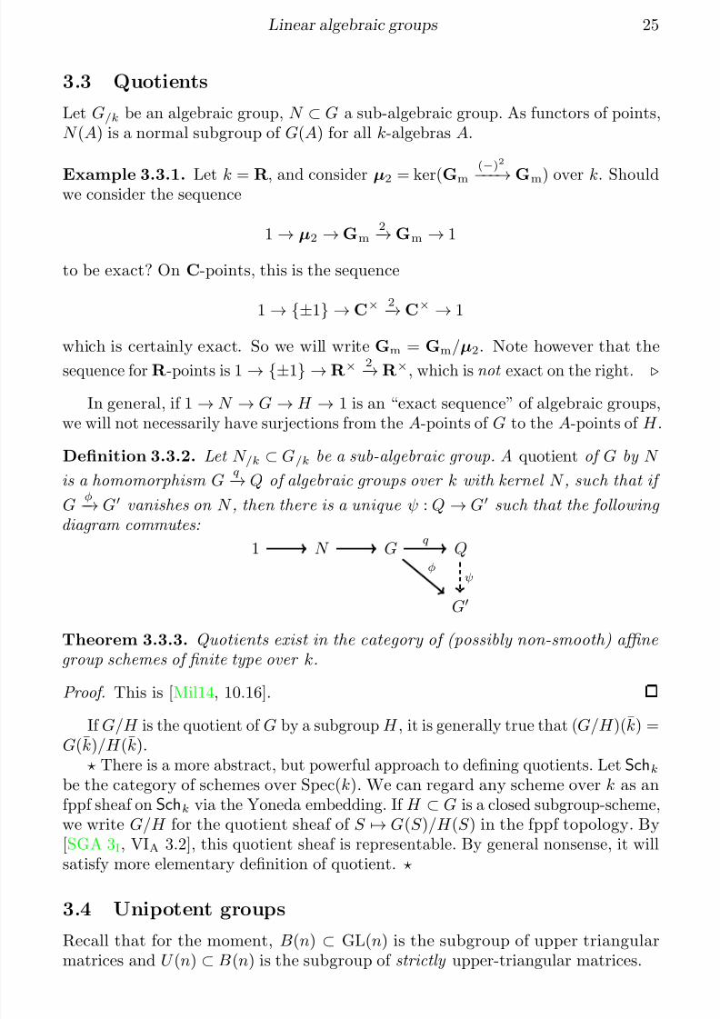
Definition 3.3.2. Let N /k ⊂ G/k be a sub-algebraic group. A quotient of G by N
is a homomorphism G q−→ Q of algebraic groups over k with kernel N , such that if
G φ−→ G vanishes on N , then there is a unique ψ : Q → G such that the following
diagram commutes:
1 N G Q
G
q
φψ
Theorem 3.3.3. Quotients exist in the category of (possibly non-smooth) affine group schemes of finite type over k.
Proof. This is [Mil14, 10.16].
If G/H is the quotient of G by a subgroup H , it is generally true that (G/H )(k) =G(k)/H (k).
There is a more abstract, but powerful approach to defining quotients. Let Schkbe the category of schemes over Spec(k). We can regard any scheme over k as anfppf sheaf on Schk via the Yoneda embedding. If H ⊂ G is a closed subgroup-scheme,we write G/H for the quotient sheaf of S → G(S )/H (S ) in the fppf topology. By[SGA 3I, VIA 3.2], this quotient sheaf is representable. By general nonsense, it willsatisfy more elementary definition of quotient.
3.4 Unipotent groups
Recall that for the moment, B(n) ⊂ GL(n) is the subgroup of upper triangularmatrices and U (n) ⊂ B(n) is the subgroup of strictly upper-triangular matrices.
7/18/2019 Linear algebraic groups and their Lie algebras
http://slidepdf.com/reader/full/linear-algebraic-groups-and-their-lie-algebras 26/81
Linear algebraic groups 26
Recall that in our filtration of B(n) ⊂ GL(n), we had B(n)/U (n) Gnm, and all
further quotients were Gra for varying r. We’d like to generalize this to an arbitrary
connected solvable groups over algebraically closed fields. For the moment though,k need not be algebraically closed.
Definition 3.4.1. Let G/k be an algebraic group. We say G is unipotent if it admits a filtration G = G0 ⊃ · · · ⊃ Gn = 1 of closed subgroups defined over k such that
1. each Gi+1 is normal in Gi,
2. each Gi/Gi+1 is isomorphic to a closed subgroup of Ga.
Clearly, unipotent groups are solvable. If k has characteristic zero, we can assumeGi/Gi+1 Ga. If k has characteristic p > 0, then we have to worry about things
like α p = ker(Ga p
−→ Ga). Fortunately, by [SGA 3II, XVII 1.5], the only possible
closed subgroups of Ga over a field of characteristic p are 0, Ga and extensions of (Z/p)r by α pe .
Theorem 3.4.2. Let G/k be a connected linear algebraic group. Then G is unipotent if and only if it is isomorphic to a closed subgroup of some U (n)/k.
Proof. This follows directly from [SGA 3II, XVII 3.5].
If G/k is unipotent and ρ : G → GL(V ) is a representation, then for all g ∈ G(k),the matrix ρ(g) is unipotent, i.e. (ρ(g)
−1)n = 0 for some n 1. Indeed, by [SGA
3II, XVII 3.4], for any such representation, there is a G-stable filtration fil• V forwhich the action of G on gr•(V ) is trivial. In other words, ρ is conjugate to arepresentation which factors through some U (n), and elements of U (n)(k) are allunipotent. Conversely, by [SGA 3II, XVII 3.8], if k is algebraically closed and everyelement of G(k) ⊂ GLn(k) is unipotent, then G is unipotent when considered as analgebraic group.
Theorem 3.4.3. Let G/k be a connected solvable smooth group over a perfect field k. Then there exists a unique connected normal Gu ⊂ G such that
1. Gu is unipotent,
2. G/Gu is of multiplicative type .
Proof. This is [Mil14, XVII 17.23].
Recall that an algebraic group G/k is of multiplicative type if it is locally (in thefpqc topology) the form A → hom(M, A×), for M an (abstract) abelian group [SGA3II, IX 1.1]. Over a perfect field, any group of multiplicative type is locally of thisform after an etale base change. In particular, if k has characteristic zero, G/Gu
will be a torus. If moreover k = k, then G/Gu Grm. In general, G/Gu will be a
closed subgroup of a torus.
Example 3.4.4. If G = B(n) ⊂ GL(n), then Gu = U (n), the subgroup of strictlyupper-triangular matrices.
7/18/2019 Linear algebraic groups and their Lie algebras
http://slidepdf.com/reader/full/linear-algebraic-groups-and-their-lie-algebras 27/81
Linear algebraic groups 27
3.5 Review of canonical filtration
For this section, assume k is a perfect field.Let G/k be a smooth connected linear algebraic group. In [cite], we defined RG,
the radical of G, to be the largest normal subgroup of G that is connected and
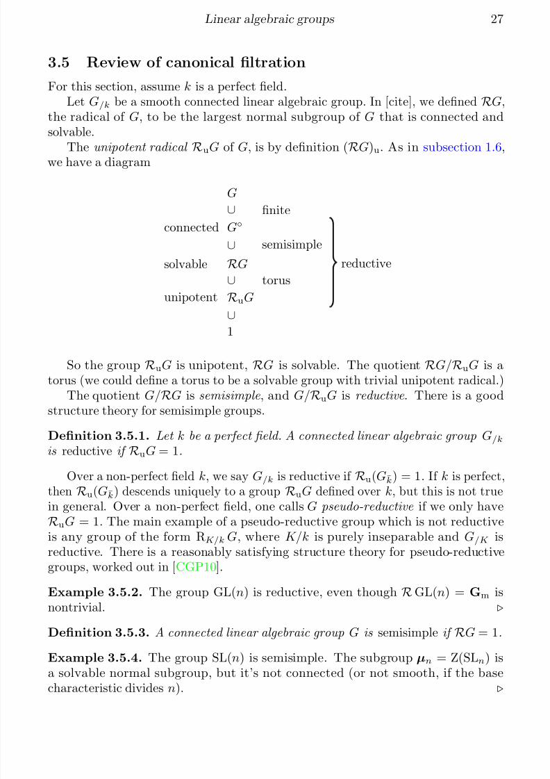
solvable.The unipotent radical RuG of G, is by definition (RG)u. As in subsection 1.6,we have a diagram
G
∪ finite
connected G◦
∪ semisimple
solvable R
G∪ torus
unipotent RuG
∪1
reductive
So the group RuG is unipotent, RG is solvable. The quotient RG/RuG is atorus (we could define a torus to be a solvable group with trivial unipotent radical.)
The quotient G/
RG is semisimple , and G/
RuG is reductive . There is a good
structure theory for semisimple groups.
Definition 3.5.1. Let k be a perfect field. A connected linear algebraic group G/k
is reductive if RuG = 1.
Over a non-perfect field k, we say G/k is reductive if Ru(Gk) = 1. If k is perfect,then Ru(Gk) descends uniquely to a group RuG defined over k, but this is not truein general. Over a non-perfect field, one calls G pseudo-reductive if we only haveRuG = 1. The main example of a pseudo-reductive group which is not reductiveis any group of the form RK/k G, where K/k is purely inseparable and G/K isreductive. There is a reasonably satisfying structure theory for pseudo-reductivegroups, worked out in [CGP10].
Example 3.5.2. The group GL(n) is reductive, even though R GL(n) = Gm isnontrivial.
Definition 3.5.3. A connected linear algebraic group G is semisimple if RG = 1.
Example 3.5.4. The group SL(n) is semisimple. The subgroup µn = Z(SLn) isa solvable normal subgroup, but it’s not connected (or not smooth, if the basecharacteristic divides n).
7/18/2019 Linear algebraic groups and their Lie algebras
http://slidepdf.com/reader/full/linear-algebraic-groups-and-their-lie-algebras 28/81
Linear algebraic groups 28
3.6 Jordan decomposition
To begin with, let k be an algebraically closed field, V a finite-dimensional k-vectorspace. Let x ∈ gl(V ). Then we can consider the action of a polynomial ring k[x] onV via x. By the fundamental theorem of finitely generated modules over a principal
ideal domain [Alg4–7, VII §2.2 thm.1], we have V = λ V λ, where for λ ∈ k, wedefineV λ = {v ∈ V : (x − λ)nv = 0 for some n 1}.
The λ for which V λ = 0 are called eigenvalues of x, and dim(V λ) is the multiplicity of λ. By a further application of the fundamental theorem for modules over a PID,we get that each V λ
i k[x]/(x − λ)ni .
The k-vector space k[x]/(t − λ)n has basis {vi = (t − λ)n−i}ni=1. Moreover,
tv1 = λv1
tv2 = λv2 + v2 · · ·When we write x with respect to this basis, we get the n × n matrix J n(λ) which isλ along the diagonal, 1 just above the diagonal, and zeros everywhere else.
For a general endomorphism x ∈ gl(V ), we end up with a direct sum decomposi-tion (with respect to some basis) g =
J ni(λi).
In all of this, we used k = k. Over a general field k, we’ll be able to write amatrix x as the sum of a diagonal matrix and a strictly upper triangular (hencenilpotent) matrix. Suppose we have written x = xss + xn, where xss is diagonal and
xn is nilpotent. It turns out that xss is uniquely determined, and is a polynomial inx. That is, there exists a polynomial f ∈ k[x], possibly depending on x, such thatxss = f (x), and similarly for xn.
For the remainder of this section, let k be an arbitrary perfect field, V a finite-dimensional k-vector space.
Definition 3.6.1. An element x ∈ gl(V ) is semisimple if it is diagonalizable after base-change to an extension of k.
Definition 3.6.2. An element x ∈
gl(V ) is nilpotent if xn = 0 for some n 1.
Definition 3.6.3. An element x ∈ GL(V ) is unipotent if x − 1 is nilpotent.
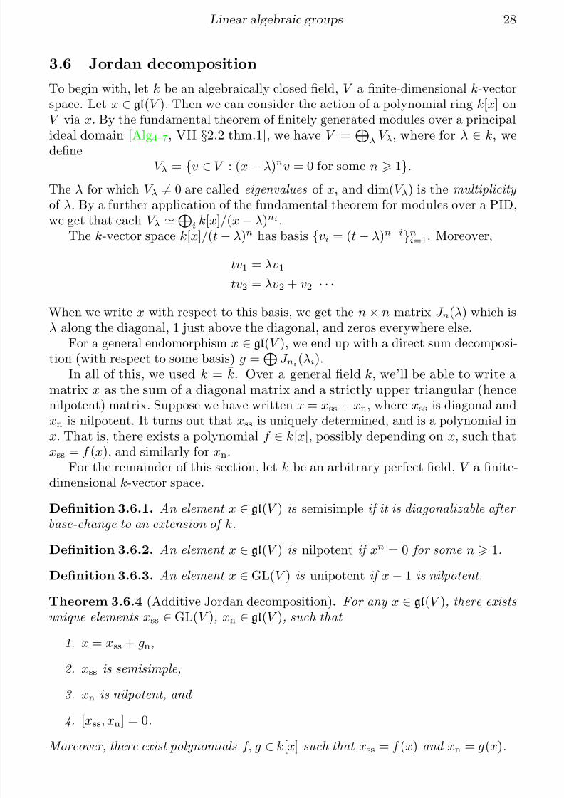
Theorem 3.6.4 (Additive Jordan decomposition). For any x ∈ gl(V ), there exists unique elements xss ∈ GL(V ), xn ∈ gl(V ), such that
1. x = xss + gn,
2. xss is semisimple,
3. xn is nilpotent, and 4. [xss, xn] = 0.
Moreover, there exist polynomials f, g ∈ k[x] such that xss = f (x) and xn = g(x).
7/18/2019 Linear algebraic groups and their Lie algebras
http://slidepdf.com/reader/full/linear-algebraic-groups-and-their-lie-algebras 29/81
Linear algebraic groups 29
Proof. Case 1: the eigenvalues of x lie in k. Then by the theory of Jordan normalform, we get existence of a decomposition. Suppose x = xss + xn = yss + yn are twodistinct decompositions. Then yss − yss = −yn + hn, and xss, xn commute with tss,tn. This is because xss and xn are polynomials in x. It follows that −xn + yn isnilpotent. The matrices xss, yss commute, so they are simultaneously diagonalizable.
So xss − yss is still semisimple. But xss − yss is also nilpotent, so xss = yss.Case 2: the eigenvalues of x may not lie in k. Take a Galois extension K/k
containing all the eigenvalues of x. (For example, we could let K be the extensionof k generated by the eigenvalues of x.) We can write x = xss + xn, where xss, xn ∈gl(V ) ⊗ K . For any σ ∈ Gal(K/k), we have σ(x) = x, because x ∈ gl(V ). But thenx = σ(xss) + σ(xn), and this is another additive Jordan decomposition of x. Byuniqueness in the first case, we see that xss and xn are fixed by σ. Since σ wasarbitrary, xss and xn lie in gl(V ).
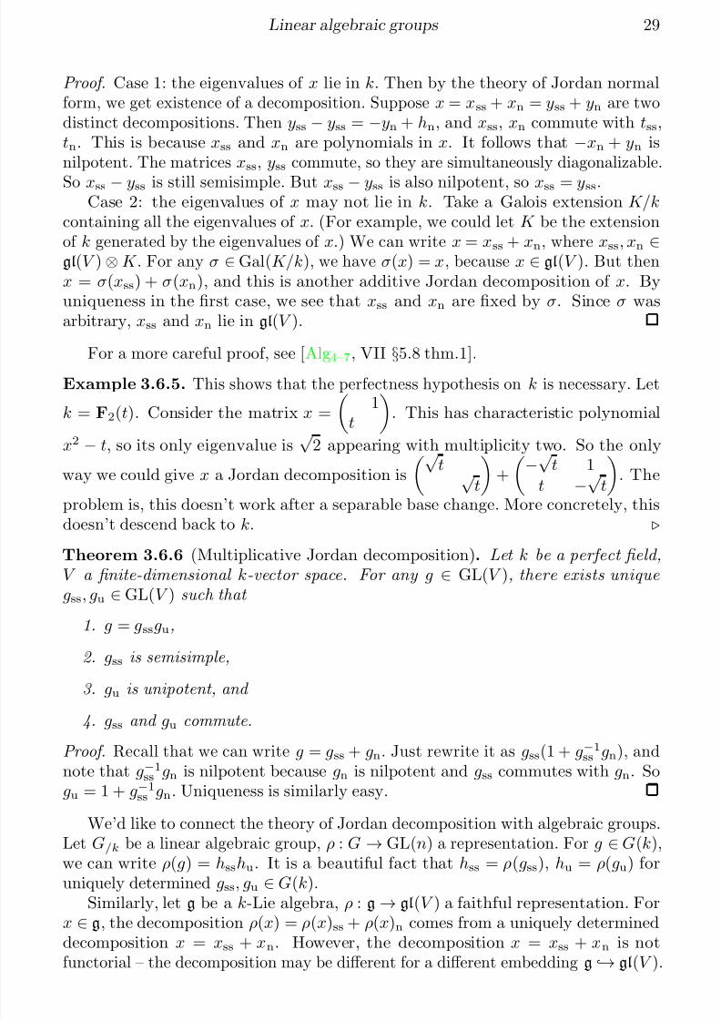
For a more careful proof, see [Alg4–7, VII §5.8 thm.1].Example 3.6.5. This shows that the perfectness hypothesis on k is necessary. Let
k = F2(t). Consider the matrix x =
1
t
. This has characteristic polynomial
x2 − t, so its only eigenvalue is√
2 appearing with multiplicity two. So the only
way we could give x a Jordan decomposition is
√ t √
t
+
−√ t 1
t −√ t
. The
problem is, this doesn’t work after a separable base change. More concretely, thisdoesn’t descend back to k.
Theorem 3.6.6 (Multiplicative Jordan decomposition). Let k be a perfect field,V a finite-dimensional k-vector space. For any g ∈ GL(V ), there exists unique gss, gu ∈ GL(V ) such that
1. g = gssgu,
2. gss is semisimple,
3. gu is unipotent, and
4. gss and gu commute.
Proof. Recall that we can write g = gss + gn. Just rewrite it as gss(1 + g−1ss gn), and
note that g−1ss gn is nilpotent because gn is nilpotent and gss commutes with gn. So
gu = 1 + g−1ss gn. Uniqueness is similarly easy.
We’d like to connect the theory of Jordan decomposition with algebraic groups.Let G/k be a linear algebraic group, ρ : G → GL(n) a representation. For g ∈ G(k),we can write ρ(g) = hsshu. It is a beautiful fact that hss = ρ(gss), hu = ρ(gu) foruniquely determined gss, gu
∈ G(k).
Similarly, let g be a k-Lie algebra, ρ : g → gl(V ) a faithful representation. Forx ∈ g, the decomposition ρ(x) = ρ(x)ss + ρ(x)n comes from a uniquely determineddecomposition x = xss + xn. However, the decomposition x = xss + xn is notfunctorial – the decomposition may be different for a different embedding g → gl(V ).
7/18/2019 Linear algebraic groups and their Lie algebras
http://slidepdf.com/reader/full/linear-algebraic-groups-and-their-lie-algebras 30/81
Linear algebraic groups 30
Let f : G → H be a homomorphism of linear algebraic groups defined overa perfect field k. Let g ∈ G(k). Then f (g)ss = f (gss) and f (g)u = f (gu). Inother words, the Jordan decomposition is functorial. It follows that if G/k is anaffine algebraic group (without a choice of embedding G → GL(n)), then themultiplicative Jordan decomposition within G is well-defined, independent of any
choice of embedding.
3.7 Diagonalizable groups
Let k be a field; recall that we are working in the category of fppf sheaves on Schk.The affine line A1(S ) = Γ(S,O S ) is such a sheaf. We have already written Ga
for the affine line considered as an algebraic group. Since Γ(S,O S ) is naturally acommutative ring, we can consider A1 as a ring scheme , i.e. a commutative ringobject in the category of schemes. We will write O for A1 so considered.
Thus if G/k is an affine algebraic group, the coordinate ring of G is
O (G) = hom(G, A1).
We will be interested in
X∗(G) = homGrp/k(G, Gm) ⊂ O (G),
the set of characters of G.
Lemma 3.7.1. The set X∗(G) is linearly independent in O (G).
Proof. We may assume k is algebraically closed. Let χ1, . . . , χn be distinct charactersof G, and suppose there is some relation
ciχi = 0 in O (G) with the ci ∈ k. If
n = 1, there is nothing to prove. In the general case, we may assume c1 = 0. Thereexists a k-algebra A and h ∈ G(A) such that χ1(h) = χn(h). Note that
ciχn(h)χi(g) =
ciχi(h)χi(g) = 0,
for all g ∈ G. This implies
n−1i=1
ci(χn(h) − χi(h))χi(g) = 0
for all g ∈ G(B) for A-algebras B. Thus χ1, . . . , χn−1 are linearly dependent inO (G)⊗kA. The only way this can happen is for χ1, . . . , χn−1 to be linearly dependentin O (G). Induction yields a contradiction.
The set X∗(G) naturally has the structure of a group, coming from the grouplaw on Gm. If χ1, χ2
∈ X(G), then
(χ1 + χ2)(g) = χ1(g)χ2(g).
Warning : this notation is confusing, because the group law in Gm is writtenmultiplicatively. But the group law on X∗(G) will always be written additively.
7/18/2019 Linear algebraic groups and their Lie algebras
http://slidepdf.com/reader/full/linear-algebraic-groups-and-their-lie-algebras 31/81
Linear algebraic groups 31
Example 3.7.2. As an exercise, check that X∗(Ga) = 0.
Example 3.7.3. One has X∗(SL2) = 0. More generally, X∗(SLn) = 0 for all n.
Example 3.7.4. Let’s compute X∗(Gm) = homGrp(Gm, Gm). We claim thatX∗(Gm)
Z as a group, with n
∈ Z corresponding to the character t
→ tn.
Indeed, O (Gm) = k[t±1], so we have to classify elements f ∈ k[t±1] such that∆(f ) = f ⊗ f . It is easy to check that these are precisely the powers of t. Alterna-tively, use the fact that O (G) has a basis consisting of the obvious characters; bylinear independence of characters, these are the only ones.
It is easy to check that X∗(G1 × G2) = X∗(G1) ⊕ X∗(G2). Thus X∗(Gnm) = Zn.
A tuple a = (a1, . . . , an) ∈ Zn corresponds to the character (t1, . . . , tn) → taii .
Example 3.7.5. There is a canonical isomorphism X∗(µn) = Z/n, even if n is notinvertible in k. There is an obvious inclusion Z/n
→ X(µn) sending a
∈ Z/n to the
character t → ta. This inclusion is an isomorphism.
In classical texts, if the base field has characteristic p > 0, then X(µ p) = 0because they only treat k-points. In fact, in such texts, they have “µ p = 1.”
From Example 3.7.4 and Example 3.7.5, we see that all finitely generated abeliangroups arise as X(G) for some G.
Theorem 3.7.6. Let G/k be a linear algebraic group. Then the following are equivalent:
1. G is isomorphic to a closed subgroup of some Gnm.
2. X∗(G) is a finitely generated abelian group, and forms a k-basis for O (G).
3. Any representation ρ : G → GL(n) is a direct sum of one-dimensional repre-sentations.
Proof. 1 ⇒ 2. An embedding G → Gnm induces a surjection O (Gn
m) O (G). Theimage in O (G) of a character χ ∈ O (Gn
m) is a character, and O (Gnm) has a basis
consisting of characters. The image of a basis is a generating set, so we’re done.
Alternatively, see [Mil14, 14.8].2 ⇒ 3. This is [Mil14, 14.11].3 ⇒ 1. By Theorem 2.6.1, there exists an embedding G → GL(n), and by 3,
we can assume the image of G lies in the subgroup of diagonal matrices, which isisomorphic to Gn
m.
Definition 3.7.7. Let G be a linear algebraic group. If G satisfies any of the equivalent conditions of Theorem 3.7.6 , we say that G is diagonalizable.
It is possible to classify diagonalizable groups. Let M be a finitely generated
abelian group, whose group law is written multiplicatively. The basic idea isto construct an algebraic group D(M ) such that there is a natural isomorphismX∗(D(M )) = M . We first define D(M ) as a functor Algk → Grp by
D(M )(A) = homGrp(M, A×).
7/18/2019 Linear algebraic groups and their Lie algebras
http://slidepdf.com/reader/full/linear-algebraic-groups-and-their-lie-algebras 32/81
Linear algebraic groups 32
This is representable, with coordinate ring the group ring
k[M ] =
m∈M
cm · m : cm = 0 for only finitely many m
.
In other words, k[M ] is the free k-vector space on M . Addition is formal, andmultiplication is defined by (c1m1)(c2m2) = c1c2(m1m2), the multiplication m1m2
taking place in M . It is easy to check that D(M )(A) = hom(k[M ], A).There is a canonical isomorphism X∗(D(M )) = M . Given m ∈ X∗(D(M )), we
get a character χm : D(M ) → Gm defined on A-points by
χm(φ) = φ(m) (φ : M → A×).
We will see that this is an isomorphism.The operation “take D(
−)” is naturally a contravariant functor from the category
of finitely generated abelian groups to the category of diagonalizable groups over k.By [SGA 3II, VIII 1.6], it induces an (anti-) equivalence of categories
D : {f.g. ab. groups} {diagonalizable gps. over k} : X∗ .
So diagonalizable groups are exactly those of the form D(M ) for a finitely generatedabelian group M . More concretely, every diagonalizable group will be of the form
Gnm × µn1 × · · · × µnr .
3.8 Tori
Let k be a field. Recall that we have an equivalence of categories:
X∗ : {diagonalizable groups /k} {f.g. ab. groups} : D .
Here X∗(G) =∗ hom(G, Gm) and D(M )(A) = hom(M, A×).
Definition 3.8.1. An algebraic group G/k has multiplicative type if Gk is diago-nalizable.
The general definition is in [SGA 3III , IX 1.1]. An affine group scheme G/S
is said to be of multiplicative type if there is an fpqc cover S → S such that GS
is diagonalizable. One says G is isotrivial if S → S may be taken to be a finiteetale cover. By [SGA 3II, X 5.16], all groups of multiplicative type over a field areisotrivial. So if G/k is of multiplicative type, there exists a finite separable extensionK/k such that GK is diagonalizable.
Definition 3.8.2. An algebraic group G/k is a split torus if G Gnm for some n.
The group G is a torus if Gk is a split torus over k.
As above, the general definition in [SGA 3II, IX 1.3] is that G/S is a torus if thereis an fpqc cover S → S such that GS Gn
m/S . As with groups of multiplicative
type, if T /k is a torus, then there is a finite separable extension K/k such thatT K Gn
m/K .
7/18/2019 Linear algebraic groups and their Lie algebras
http://slidepdf.com/reader/full/linear-algebraic-groups-and-their-lie-algebras 33/81
Linear algebraic groups 33
Example 3.8.3 (Nonsplit tori). Recall that if K/k is a field extension and G/K is analgebraic group, then the Weil restriction RK/k G is the algebraic group representingthe functor A → G(A ⊗k K ) on k-algebras A. Consider G = RK/k Gm. For anyk-algebra A, we have (by definition) G(A) = (A ⊗k K )×. Note that G(A) acts onK A via multiplication, so there is an embedding RK/k Gm
→ GL(K )/k. If K/k is
Galois, there is a canonical isomorphism of k-algebras K ⊗k K ∼−→ Γ K , whereΓ = Gal(K/k). It sends x ⊗ y to the tuple (xγ (y))γ . Now for A ∈ AlgK , we compute
G(A ⊗k K ) = G(A ⊗K (K ⊗k K ))
= G
A ⊗K
Γ
K
=
ΓG(A).
Thus (RK/k Gm)K =
Γ Gm/K , hence RK/k Gm is a torus. But RK/k Gm isnot diagonalizable. If it were, by Theorem 3.7.6 the representation RK/k Gm →GL(K )/k would factor through the diagonal, whence all coordinates of the image of (RK/k Gm)(k) = K × would be in k, which is clearly false.
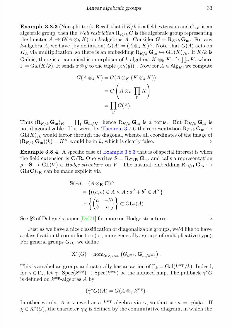
Example 3.8.4. A specific case of Example 3.8.3 that is of special interest is whenthe field extension is C/R. One writes S = RC/RGm, and calls a representationρ : S → GL(V ) a Hodge structure on V . The natural embedding RC/RGm →GL(C)/R can be made explicit via
S(A) = (A ⊗R C)×
= {((a, b) ∈ A × A : a2 + b2 ∈ A×}
a −bb a
⊂ GL2(A).
See §2 of Deligne’s paper [Del71] for more on Hodge structures.
Just as we have a nice classification of diagonalizable groups, we’d like to havea classification theorem for tori (or, more generally, groups of multiplicative type).For general groups G/k, we define
X∗(G) = homGrp/ksep
Gksep, Gm/ksep
.
This is an abelian group, and naturally has an action of Γk = Gal(ksep/k). Indeed,for γ ∈ Γk, let γ : Spec(ksep) → Spec(ksep) be the induced map. The pullback γ ∗Gis defined on ksep-algebras A by
(γ ∗G)(A) = G(A ⊗γ ksep).
In other words, A is viewed as a ksep-algebra via γ , so that x · a = γ (x)a. If χ ∈ X∗(G), the character γχ is defined by the commutative diagram, in which the
7/18/2019 Linear algebraic groups and their Lie algebras
http://slidepdf.com/reader/full/linear-algebraic-groups-and-their-lie-algebras 34/81
Linear algebraic groups 34
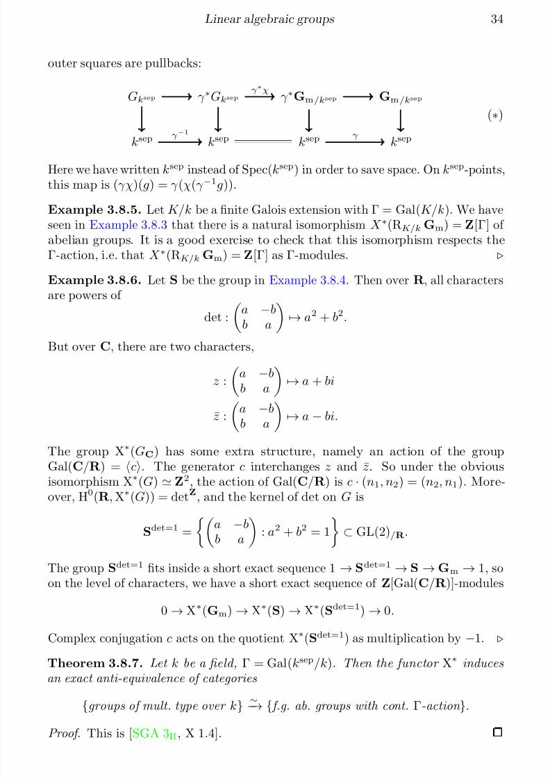
outer squares are pullbacks:
Gksep γ ∗Gksep γ ∗Gm/ksep Gm/ksep
ksep ksep ksep ksep
γ ∗χ
γ −1
γ
(∗)
Here we have written ksep instead of Spec(ksep) in order to save space. On ksep-points,this map is (γχ)(g) = γ (χ(γ −1g)).
Example 3.8.5. Let K/k be a finite Galois extension with Γ = Gal(K/k). We haveseen in Example 3.8.3 that there is a natural isomorphism X ∗(RK/k Gm) = Z[Γ] of abelian groups. It is a good exercise to check that this isomorphism respects theΓ-action, i.e. that X ∗(RK/k Gm) = Z[Γ] as Γ-modules.
Example 3.8.6. Let S be the group in Example 3.8.4. Then over R, all charactersare powers of
det :
a −bb a
→ a2 + b2.
But over C, there are two characters,
z :
a −bb a
→ a + bi
z : a −bb a
→ a − bi.
The group X∗(GC) has some extra structure, namely an action of the groupGal(C/R) = c. The generator c interchanges z and z. So under the obviousisomorphism X∗(G) Z2, the action of Gal(C/R) is c · (n1, n2) = (n2, n1). More-over, H0(R, X∗(G)) = detZ, and the kernel of det on G is
Sdet=1 = a −b
b a : a2 + b2 = 1 ⊂ GL(2)/R.
The group Sdet=1 fits inside a short exact sequence 1 → Sdet=1 → S → Gm → 1, soon the level of characters, we have a short exact sequence of Z[Gal(C/R)]-modules
0 → X∗(Gm) → X∗(S) → X∗(Sdet=1) → 0.
Complex conjugation c acts on the quotient X∗(Sdet=1) as multiplication by −1.
Theorem 3.8.7. Let k be a field, Γ = Gal(ksep/k). Then the functor X∗ induces
an exact anti-equivalence of categories
{groups of mult. type over k} ∼−→ { f.g. ab. groups with cont. Γ-action }.
Proof. This is [SGA 3II, X 1.4].
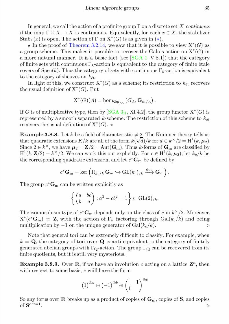
7/18/2019 Linear algebraic groups and their Lie algebras
http://slidepdf.com/reader/full/linear-algebraic-groups-and-their-lie-algebras 35/81
Linear algebraic groups 35
In general, we call the action of a profinite group Γ on a discrete set X continuous if the map Γ × X → X is continuous. Equivalently, for each x ∈ X , the stabilizerStabΓ(x) is open. The action of Γ on X∗(G) is as given in (∗).
In the proof of Theorem 3.2.14, we saw that it is possible to view X∗(G) asa group scheme. This makes it possible to recover the Galois action on X∗(G) in
a more natural manner. It is a basic fact (see [SGA 1, V 8.1]) that the categoryof finite sets with continuous Γk-action is equivalent to the category of finite etalecovers of Spec(k). Thus the category of sets with continuous Γk-action is equivalentto the category of sheaves on ket.
In light of this, we construct X∗(G) as a scheme; its restriction to ket recoversthe usual definition of X∗(G). Put
X∗(G)(A) = homGrp/A
GA, Gm/A
.
If G is of multiplicative type, then by [SGA 3II, XI 4.2], the group functor X∗
(G) isrepresented by a smooth separated k-scheme. The restriction of this scheme to ket
recovers the usual definition of X∗(G).
Example 3.8.8. Let k be a field of characteristic = 2. The Kummer theory tells usthat quadratic extensions K/k are all of the form k(
√ d)/k for d ∈ k×/2 = H1(k, µ2).
Since 2 ∈ k×, we have µ2 = Z/2 = Aut(Gm). Thus k-forms of Gm are classified byH1(k, Z/2) = k×/2. We can work this out explicitly. For c ∈ H1(k, µ2), let kc/k bethe corresponding quadratic extension, and let c∗Gm be defined by
c∗Gm = kerRkc/k Gm → GL(kc)/k det−−→ Gm .
The group c∗Gm can be written explicitly asa bcb a
: a2 − cb2 = 1
⊂ GL(2)/k.
The isomorphism type of c∗Gm depends only on the class of c in k×/2. Moreover,X∗(c∗Gm) Z, with the action of Γk factoring through Gal(kc/k) and being
multiplication by −1 on the unique generator of Gal(kc/k). Note that general tori can be extremely difficult to classify. For example, when
k = Q, the category of tori over Q is anti-equivalent to the category of finitelygenerated abelian groups with ΓQ-action. The group ΓQ can be recovered from itsfinite quotients, but it is still very mysterious.
Example 3.8.9. Over R, if we have an involution c acting on a lattice Zn, thenwith respect to some basis, c wiill have the form
1⊕a ⊕ −1⊕b ⊕ 11 ⊕cSo any torus over R breaks up as a product of copies of Gm, copies of S, and copiesof Sdet=1.
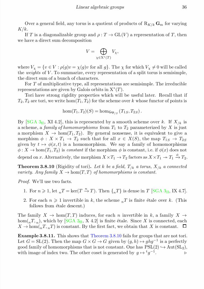
7/18/2019 Linear algebraic groups and their Lie algebras
http://slidepdf.com/reader/full/linear-algebraic-groups-and-their-lie-algebras 36/81
Linear algebraic groups 36
Over a general field, any torus is a quotient of products of RK/k Gm for varyingK/k.
If T is a diagonalizable group and ρ : T → GL(V ) a representation of T , thenwe have a direct sum decomposition
V = χ∈X∗(T )
V χ,
where V χ = {v ∈ V : ρ(g)v = χ(g)v for all g}. The χ for which V χ = 0 will be calledthe weights of V . To summarize, every representation of a split torus is semisimple,the direct sum of a bunch of characters.
For T of multiplicative type, all representations are semisimple. The irreduciblerepresentations are given by Galois orbits in X∗(T ).
Tori have strong rigidity properties which will be useful later. Recall that if
T 2, T 2 are tori, we write hom(T 1, T 2) for the scheme over k whose functor of points is
hom(T 1, T 2)(S ) = homGrp/S (T 1S , T 2S ) .
By [SGA 3II, XI 4.2], this is represented by a smooth scheme over k. If X /k isa scheme, a family of homomorphisms from T 1 to T 2 parameterized by X is justa morphism X → hom(T 1, T 2). By general nonsense, it is equivalent to give amorphism φ : X × T 1 → T 2 such that for all x ∈ X (S ), the map T 1S → T 2S given by t → φ(x, t) is a homomorphism. We say a family of homomorphisms
φ : X → hom(T 1, T 2) is constant if the morphism φ is constant, i.e. if φ(x) does notdepend on x. Alternatively, the morphism X ×T 1 → T 2 factors as X ×T 1 T 1
φ−→ T 2.
Theorem 3.8.10 (Rigidity of tori). Let k be a field, T /k a torus, X /k a connected variety. Any family X → hom(T, T ) of homomorphisms is constant.
Proof. We’ll use two facts.
1. For n 1, let nT = ker(T n−→ T ). Then {nT } is dense in T [SGA 3II, IX 4.7].
2. For each n
1 invertible in k, the scheme nT is finite etale over k. (Thisfollows from etale descent.)
The family X → hom(T, T ) induces, for each n invertible in k, a family X →hom(nT, n), which by [SGA 3II, X 4.2] is finite etale. Since X is connected, eachX → hom(nT, nT ) is constant. By the first fact, we obtain that X is constant.
Example 3.8.11. This shows that Theorem 3.8.10 fails for groups that are not tori.Let G = SL(2). Then the map G × G → G given by (g, h) → ghg−1 is a perfectlygood family of homomorphisms that is not constant. One has PSL(2) → Aut(SL2),
with image of index two. The other coset is generated by g → t
g−1
.
7/18/2019 Linear algebraic groups and their Lie algebras
http://slidepdf.com/reader/full/linear-algebraic-groups-and-their-lie-algebras 37/81
Linear algebraic groups 37
4 Semisimple groups
Let k be an algebraically closed field of characteristic zero. Let G/k be a reductivealgebraic group. That is, G is connected and RuG = 1. We will associate to G somecombinatorial data, called the root datum . The root datum of G will characterize G
up to isomorphism, will not depend on the field k, and will completely determinethe representation theory of G. Much of the theory will depend on the notions of maximal torus and Borel subgroup. To prove basic properties of these, we need to beable to take quotients, and it is to this that we now turn. The theory of quotientsrequires quite a bit of, sophistication, and may safely be skipped at first reading.
4.1 Quotients revisited
The “morally correct” place to take quotients is in the category of fppf sheaves.
Definition 4.1.1. A finite family {f i : X i → X } of morphisms of schemes is an fppf cover if it is jointly surjective (on points), and each X i → X is flat, of finite presentation, and quasi-finite.
We write fppf for the topology generated by fppf covers. Recall that a topologyis called subcanonical if each representable functor is a sheaf. Also, a sieve on X isa subfunctor of hX = hom(−, X ). We reproduce the following theorem from SGA.
Theorem 4.1.2.
1. A sieve S on X is a cover for the fppf topology if and only if there is an open affine cover {X i} of X together with affine fppf covers {X ij → X i} such that each X ij → X is in S .
2. A presheaf F on Sch is an fppf sheaf if and only if:
(a) F is a Zariski sheaf.
(b) For each fppf cover X → Y , where X and Y are affine, the following diagram is an equalizer:
F (X ) F (Y ) F (Y ×X Y ).
3. The fppf topology is subcanonical.
4. If {X i → X } is jointly surjective and each X i → X is faithfully flat and of finite presehtation, then {X i → X } is an fppf cover.
Proof. This is [SGA 3I, IV 6.3.1].
A good general source for topologies and sheaves is the book [MLM94]. Fromit, we get that the category Shfppf (SchS ) is a topos . That is, limits, colimits andmore exist in the category of sheaves on SchS . However, it can be quite tricky tocheck whether a given colimit of schemes (taken in the fppf topology) is actuallyrepresented by a scheme.
7/18/2019 Linear algebraic groups and their Lie algebras
http://slidepdf.com/reader/full/linear-algebraic-groups-and-their-lie-algebras 38/81
Linear algebraic groups 38
Let k be a field. For the remainder, we’ll work in the category of fppf sheaves onSchk. We’ll call such sheaves spaces .
Definition 4.1.3. Let G be a k-group space. A k-space X is called a G-space if it is equipped with a morphism G × X → X , such that for each S ∈ Schk, the map
G(S ) × X (S ) → X (S ) gives an action of the group G(S ) on the set X (S ).
If G/k is an algebraic group and X /k is a variety, we call X a G-variety , or variety with G-action . (Recall that for us, a variety over k is a separated scheme of finitetype over k.) The representability of quotients G\X is a subtle one, but fortunatelywe only need to take quotients G/H , where H ⊂ G is an algebraic subgroup.
Theorem 4.1.4. Let G/k be an algebraic group, H ⊂ G an algebraic subgroup.Then the fppf quotient G/H is a variety over k. If G is smooth, so is G/H , and if H is normal, then G/H has a unique structure of a group scheme for which G
→ G/H
is a homomorphism.
Proof. This is [SGA 3I, VIA 3.2].
A major theorem whose proof uses quotients is the Borel fixed point theorem. Tostate it, we need some terminology. Following [EGA 2, II 5.4.1], we say a morphismf : X → Y of schemes is proper if it is separated, of finite type, and if for all Y → Y ,the induced morphism X Y → Y is closed. We call a variety X /k proper if thestructure map X → Spec(k) is proper. There is a valuative criterion for properness[EGA 2, II 7.3.8]. One considers pairs (A, K ), where A is a valuation ring withmorphism Spec(A) → Y , and K is the field of fractions of Y . A morphism X → Y is proper if and only if for all such pairs, the map X /Y (A) → X /Y (K ) is a bijection.If f : X → Y is a morphism of varieties over C, then by [SGA 1, XII 3.2], f is properif and f : X (C) → Y (C) is proper in the topological sense. (Following [Top1–4, I§10.2 th.1], a map f : X → Y between Hausdorff spaces is proper if it is closed, andthe preimage of any compact set is compact.)
Theorem 4.1.5. Let k be an algebraically closed field, G/k a connected solvable group, and X /k a proper non-empty G-variety. Then X G
= ∅.
Proof. We induct on the dimension of G. If G is one-dimensional, then G is one of {Ga, Gm}, so neither G nor any of its nontrivial quotients are proper. For x ∈ X (k),let Gx = StabG(x). Either Gx = G, in which case x ∈ X G(k), or Gx is finite, inwhich case we have an embedding G/Gx → X given by g → gx. By passing to theclosure of the image of this map, we may assume the image of G/Gx in X is dense.Thus X G/Gx is a G-stable finite nonempty (because G isn’t proper) variety onwhich G acts, hence X G ⊃ X G/Gx.
In the general case, choose a one-dimensional normal subgroup H ⊂ G. By
induction, X H
= ∅, and by the first part of the proof, X G
= (X H
)G/H
= ∅.For a more careful proof, see [Mil14, 18.1].
Checking the valuative (or topological) criteria for properness can be prettydifficult. There is a special class of morphisms, called projective morphisms , that
7/18/2019 Linear algebraic groups and their Lie algebras
http://slidepdf.com/reader/full/linear-algebraic-groups-and-their-lie-algebras 39/81
Linear algebraic groups 39
are automatically proper. Let S be a base scheme, and E a quasi-coherent sheaf onS . Define a functor P(E ) on SchS by
P(E )(X ) = {(L , ϕ) : L is invertible and ϕ : E X L }/ .
That is, P(E )(X ) is the set of isomorphism classes of pairs (L , ϕ), where L is a linebundle on X and ϕ : E X L is a surjection. By [EGA 2, II 4.2.3], this functor isrepresentable. Following [EGA 2, II 5.5.2], a morphism f : X → Y is called projective if it factors as X → P(E ) Y , where E is a coherent O Y -module, X → P(E ) isa closed immersion and P(E ) Y is the canonical morphism. Equivalently, X isisomorphic to Proj(A ) for some sheaf A = A • of graded O Y -algebras, which isgenerated as an O Y -algebra by A 1, and for which A 1 is coherent. By [EGA 2, II5.5.3], projective morphisms are proper. In particular, if we work over a base field k,all closed subschemes of P(V ) for a finite-dimensional k-vector space V are proper.
You need to be careful when taking quotients. As motivation, suppose G/k is analgebraic group and Z ⊂ Z(G) is a central subgroup. For any k-algebra A, we havea long exact sequence
1 → Z (A) → G(A) → (G/Z )(A) → H1fppf (A, Z ) → · · ·
So (G/Z )(A) is “easy” to understand when Z is “cohomologically trivial” in somesense. Conversely, when Z has nontrivial cohomology, G/Z tends to be trickier tostudy directly.
Example 4.1.6. Consider the algebraic group PGL(n) = GL(n)/Gm. See [Con,1.6.3] for a careful construction. It is well-known that H1(A, Gm) = Pic(A), thegroup of isomorphism classes of invertible A-modules. Thus if A is a Dedekinddomain with non-trivial class group, the map GLn(A)/A× → PGLn(A) is not surjective. But since Pic(k) = 0 for all fields K , one has PGLn(k) = GLn(k)/k×.
Example 4.1.7. This problem presents itself even earlier with PSL(n) =“SL(n)/µn.”The problem is, by Kummer theory, H1(k, µn) = k×/n whenever n is invertible ink. So, for example, SL2(R) → PSL2(R) should not be surjective, because it has
cokernel H1
(R,µ2) = Z/2. It turns out that the quotient sheaf SL(n)/µn is actuallyPGL(n). For this reason, we will only use notation PSL(n) when taking its k-valuedpoints. See http://mathoverflow.net/questions/16145/ for more discussion of this.
4.2 Centralizers, normalizers, and transporter schemes
Here we define some constructions scheme-theoretically that will be used extensivelyin the structure theory of reductive groups. Fix a base scheme S , and let G/S be a
group scheme. If X, Y ⊂ G are subschemes, the transporter scheme TranspG(X, Y )and the strict transporter scheme stTranspG(X, Y ) are given by their functors of
7/18/2019 Linear algebraic groups and their Lie algebras
http://slidepdf.com/reader/full/linear-algebraic-groups-and-their-lie-algebras 40/81
Linear algebraic groups 40
points:
TranspG(X, Y )(T ) = {g ∈ G(T ) : ad(g)(X T ) ⊂ Y T }= {g ∈ G(T ) : gX (T )g−1 ⊂ Y (T ) for all T → T }
stTranspG(X, Y )(T ) = {g ∈ G(T ) : ad(g)(X T ) = Y T }.
Similarly, if u, v : X → G are morphisms, one defines
TranspG(u, v)(T ) = {g ∈ G(T ) : ad(g) ◦ uT = vV }.
This enables us to define, for a subgroup-scheme H ⊂ G,
CG(H ) = TranspG(H → G, H → G) (the centralizer )
NG(H ) = stTranspG(H, H ) (the normalizer ).
We reproduce the following theorem from SGA.
Theorem 4.2.1. Let k be a field, G/k a group scheme of finite type.
1. If X, Y ⊂ G are closed subschemes, then TranspG(X, Y ) and stTranspG(X, Y )are represented by closed subschemes of G.
2. If u, v : X → G are two morphisms of schemes over k, then TranspG(u, v) is represented by a closed subscheme of G.
Proof. This is essentially [SGA 3I, VIB 6.2.5].
Corollary 4.2.2. Let k be a field, G/k a group scheme of finite type, and H ⊂ G a closed subgroup scheme. Then CG(H ) and NG(H ) are represented by closed subgroupschemes of G
Clearly CG(H ) ⊂ NG(H ).
4.3 Borel subgroups
For this section, k is an algebraically closed field of characteristic zero.
Definition 4.3.1. Let G/k be a linear algebraic group. A Borel subgroup of G is a connected solvable subgroup B ⊂ G that is maximal with respect to those properties.
Theorem 4.3.2. Let G/k be a linear algebraic group. Then all Borel subgroups of G are conjugate.
Proof. Let B1, B2 be two Borel subgroups. By [Mil14, 18.11.a], the variety G/B1 is
proper. By Theorem 4.1.5, the left-action of B2 on G/B1 admits a fixed point gB1.One has B2 ⊂ ad(g)(B1); by maximality B2 = ad(g)(B1).
In general, one calls the quotient G/B of G by a Borel subgroup B the flag variety of G.
7/18/2019 Linear algebraic groups and their Lie algebras
http://slidepdf.com/reader/full/linear-algebraic-groups-and-their-lie-algebras 41/81
Linear algebraic groups 41
Example 4.3.3. If G = GL(n), then by Theorem 3.2.14, the subgroup B of upper-triangular matrices is a Borel subgroup. We will see that G/B is proper. Indeed,we will work in much greater generality. Let S be a base scheme and E a locallyfree O S -module. If X /S is a scheme, write E X for the pullback of E to X . WriteGL(E ) for the functor X
→ AutO X (E X). This is an open subscheme of V(E ∨
⊗E ),
so it is representable.Let n = rk(E ); for r < n, let Gr(E , r) be the functor given by
Gr(E , r)(X ) = {E X F : F is a locally free O X -module of rank r}/ .
By [Nit05, ex.2], this is representable. note that Gr(E , 1) = P(E ), so Gr(E , 1) isprojective. More generally, for each r the operation “take r-th wedge power” givesa closed embedding Gr(E , r) → P(
rE ), so all the Gr(E , r) are projective. Put
Gr(E ) =
r<n Gr(E , r); this is projective via the Segre embedding [EGA 2, II 4.3.3]
P(E ) × · · · × P(n−1 E ) → P(E ⊗ · · · ⊗n−1 E ).
Suppose E admits a descending filtration fil• E such that each quotient E r =E / filr has rank r. Define a closed subgroup of GL(E ) by
B(X ) = {g ∈ GL(E )(X ) : g preserves fil•}.
This is a Borel subgroup of GL(E ). We will realize the relative flag variety G/B asa closed subscheme of Gr(E ). If X /S is a scheme, a flag (relative to E ) on X is adiagram E X = V n
· · · V 0 = 0 of locally free quotients of E X , where each V r
has rank r. Write V • for such a flag. Define a functor Fl(E ) by
Fl(E )(X ) = {flags relative to E on X }/ .
The rule V • → (V r)r gives a closed embedding Fl(E ) → Gr(E ). See [DG80, I §2 6.3]for a proof when S = Spec(Z) and E = Zn.
Our filtration fil• E induces an element of Fl(E )(S ), namely {E E / filr}r. Theaction of GL(E ) on E induces a right action of GL(E ) on Fl(E ), in which an element
g ∈ GL(E )(X ) acts on a flag E V • by E g−→ E V •. Moreover, B ⊂ GL(E ) acts
trivially. Assume S is locally noetherian. Then by [SGA 3I, V 10.1.1], the quotientGL(E )/B exists and comes with an embedding GL(E )/B → Fl(E ). We claim thatthis map is surjective, hence an isomorphism. Indeed, Zariski-locally, it comes downto checking that GL(An)/B(A) → Fl(An) is surjective, which is a basic fact fromlinear algebra. Thus GL(E )/B
∼−→ Fl(E ).
We will be mainly interested in when S = Spec(k) and V = kn. In this case, wewrite Gr(n, r) = Gr(kn, r) and Fl(n) = Fl(kn). Thus GL(n)/B
∼−→ Fl(n) → Gr(n).More generally, we have the following fact.
Theorem 4.3.4. Let G be a linear algebraic group, B ⊂ G a Borel subgroup. Then G/B is a projective variety.
Definition 4.3.5. Let G be a linear algebraic group. A closed subgroup P ⊂ G is parabolic if G/P is proper.
7/18/2019 Linear algebraic groups and their Lie algebras
http://slidepdf.com/reader/full/linear-algebraic-groups-and-their-lie-algebras 42/81
Linear algebraic groups 42
Theorem 4.3.6. A subgroup P ⊂ G is parabolic if and only if P contains a Borel subgroup of G.
Proof. ⇐. Suppose P contains a Borel subgroup B. Then the inclusion B ⊂ P induces a map G/B G/P . Since G/B is proper, by [EGA 2, II 5.4.3], so is G/P .
Alternatively, see [SGA 3II, XVI 2.5] for a proof over a general base.⇒. Consider the action of B on the proper variety G/P . By Theorem 4.1.5,there is a fixed point gP . One obtains ad(g−1)(B) ⊂ P , so P contains a Borelsubgroup.
In light of this result, we could have defined a Borel subgroup to be a minimalparabolic subgroup.
4.4 Maximal tori
For this section, k is an algebraically closed field of characteristic zero. Let G/k bea linear algebraic group. A maximal torus in G is a subgroup scheme T ⊂ G that isa torus, and is maximal with respect to this property. In our setting, any torus in Gis contained in a maximal torus.
Example 4.4.1. Let G = GL(n). Then we can choose T to be the subgroupconsisting of diagonal matrices. This is a maximal torus because all tori arediagonalizable, so any torus in GL(n) is conjugate to a subgroup of T . A Borelsubgroup consists of upper-triangular matrices.
Theorem 4.4.2. Let G/k be a linear algebraic group. Then all maximal tori are conjugate.
Proof. If G is solvable, this is [Mil14, 17.40]. Essentially, one uses the fact thatG = T RuG for any maximal torus T .
If G is a general group, then different maximal tori T 1, T 2 will live in Borelsubgroups B1, B2. By Theorem 4.3.2, the subgroups B1 and B2 are conjugate, sowe may as well assume T 1 and T 2 are maximal tori in the same Borel subgroup B.But then we can use the fact that the theorem holds for solvable groups.
Example 4.4.3. Let ρ : G → GL(V ) be a representation, where G is a connectedsolvable group. Then G acts on P(V ) via GL(V ), so Theorem 4.1.5 tells us that Gfixes a vector, i.e. that V contains a G-invariant line.
Lemma 4.4.4. Let T ⊂ G be a torus. Then the quotient WG(T ) = CG(T )◦ =NG(T )◦, hence the quotient NG(T )/ CG(T ) is finite etale.
Proof. There is an obvious family NG(T )◦ × T → T given by (y, t) → yty−1. ByTheorem 3.8.10, this is constant, hence NG(T )◦
⊂ CG(T ).
One calls WG(T ) the Weyl group of the pair (G, T ). It is finite etale over k.
Lemma 4.4.5. Let G/k be a connected reductive group. Then RG = Z(G)◦.
7/18/2019 Linear algebraic groups and their Lie algebras
http://slidepdf.com/reader/full/linear-algebraic-groups-and-their-lie-algebras 43/81
Linear algebraic groups 43
Proof. Note that RG is a torus. Since RG is normal in G, there is a familyG × RG → RG given by (y, t) → yty−1. Again by Theorem 3.8.10, this is trivial,hence RG ⊂ Z(G). The result follows.
Lemma 4.4.6. Let G be a connected linear algebraic group that admits a faithful
irreducible representation ρ : G → GL(V ). Then G is reductive.
Proof. We may assume that G ⊂ GL(V ). Let H = RuG; the space V H is nonzerosince H is unipotent. In fact, since H is normal in G, V H is a subrepresentation of V . Since V is simple, V H = V . But G ⊂ GL(V ), so H = 1.
Corollary 4.4.7. The groups GL(n), SL(n), SO(2n) and Sp(2n) are reductive.
Proof. Apply Lemma 4.4.6 to the standard representations. For SO and Sp, use thefact that the group preserves a nondegenerate bilinear form.
Theorem 4.4.8. Let k be a field, G/k a reductive group. If T ⊂ G is a torus, then CG(T ) is reductive. If T is maximal, then CG(T ) = T .
Proof. This is [SGA 3III , XIX 1.6].
4.5 Root systems
Let k be a field, G/k a reductive group, g = Lie(G). In subsection 2.8, we defineda canonical representation ad : G
→ GL(g). Let T
⊂ G be a maximal torus. We
are interested in the representation ad |T : T → GL(g). For simplicity, assume T isdiagonalizable (i.e. , a split torus). By Theorem 3.7.6, there is a decomposition
g =
α∈X∗(T )
gα,
where for α ∈ X∗(T ), the space gα = {x ∈ g : tg = α(t)g for all t ∈ T }. LetR(G, T ) = {α ∈ X∗(T ) 0 : gα = 0}. Then we have a decomposition
g = g0 ⊕ α∈R(G,T )
gα.
We call R(G, T ) ⊂ X∗(G) the set of roots of G. This is a finite set.Let V be the span of R(G, T ) in X∗(T )R = X∗(T ) ⊗ R. The finite set R(G, T )
sitting inside the real vector space V is an example of a “root system.” Generalroot systems break up into irreducibles, and there is a combinatorial classificationof irreducible root systems into types An, Bn, Cn, Dn, G2, F4, E6, E7, E8. The rootsystem R(G, T ) ⊂ V will recover G/ Z(G).
7/18/2019 Linear algebraic groups and their Lie algebras
http://slidepdf.com/reader/full/linear-algebraic-groups-and-their-lie-algebras 44/81
Linear algebraic groups 44
Example 4.5.1. We will work out the root datum of SL(n + 1) for n 1. Wechoose the maximal torus
T =
diag(a1, . . . , an+1) : ai ∈ Gm and
ai = 1
=∗ . . .
∗ ⊂ SL(n + 1).
Define χi : T → Gm by χi(diag(a1, . . . , an+1)) = ai. Then (χ1, . . . , χn) induces anisomorphism between T and the subgroup of Gn+1
m consisting of (a1, . . . , an+1) witha1 · · · an+1) = 1. Thus X∗(T ) = { aiχi :
ai = 0}.
The Lie algebra sl(n + 1) is spanned by t = Lie(T ) and the set
{E i,j = (δ i,aδ j,b)a,b} ⊂ sl(n + 1).Moreover, one can check that
ad (diag(a1, . . . , an+1)) (E i,j) = aiaj
E i,j.
Thus, the root decomposition of sl(n + 1) is
sl(n + 1) = t ⊕i=j
E i,j.
So R(SLn+1, T ) = {χi − χj : i = j}. We think of R(SLn+1) as a subset of the realvector space { aiχi : ai ∈ R and
ai = 0}.
With this example in mind, we move towards the general definition of a rootsystem. Fix a finite-dimensional R-vector space V . For α ∈ V 0, a reflection onV with vector α is a linear map s : V → V such s(α) = −α, and for which thereexists a decomposition V = Rα ⊕ U such that α|U = 1. Note that if s is a reflectionwith vector α, then s(v) − v ∈ Rα for all v ∈ V .
Lemma 4.5.2. Let V be a finite-dimensional R-vector space, R ⊂ V a finite set which spans V , and α ∈ V 0. There exists at most one reflection s of V with vector α such that s(R) = R.
Proof. This is [Lie4–6, VI §1.1 lem.1]. Suppose s, s are two such reflections. Defineu = s(s)−1. Note that u(α) = α. Moreover, u induces the identity on V /α. Thisimplies u is unipotent. But u(R) = R, so un = 1 for some n 1. This means that uis semisimple. The only way an operator can be both unipotent and semisimple isfor u = 1.
Definition 4.5.3. Let V be a finite-dimensional R-vector space. A subset R ⊂ V 0is a root system in V if the following hold:
1. R is finite and spans V .
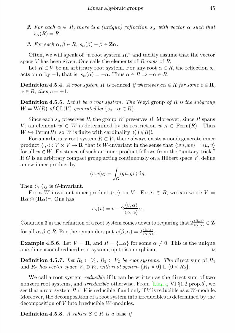
7/18/2019 Linear algebraic groups and their Lie algebras
http://slidepdf.com/reader/full/linear-algebraic-groups-and-their-lie-algebras 45/81
Linear algebraic groups 45
2. For each α ∈ R, there is a (unique) reflection sα with vector α such that sα(R) = R.
3. For each α, β ∈ R, sα(β ) − β ∈ Zα.
Often, we will speak of “a root system R,” and tacitly assume that the vectorspace V has been given. One calls the elements of R roots of R.
Let R ⊂ V be an arbitrary root system. For any root α ∈ R, the reflection sαacts on α by −1, that is, sα(α) = −α. Thus α ∈ R ⇒ −α ∈ R.
Definition 4.5.4. A root system R is reduced if whenever cα ∈ R for some c ∈ R,α ∈ R, then c = ±1.
Definition 4.5.5. Let R be a root system. The Weyl group of R is the subgroupW = W(R) of GL(V ) generated by {sα : α ∈ R}.
Since each sα preserves R, the group W preserves R. Moreover, since R spansV , an element w ∈ W is determined by its restriction w|R ∈ Perm(R). ThusW → Perm(R), so W is finite with cardinality (#R)!.
For an arbitrary root system R ⊂ V , there always exists a nondegenerate innerproduct ·, · : V × V → R that is W -invariant in the sense that wu,wv = u, vfor all w ∈ W . Existence of such an inner product follows from the “unitary trick.”If G is an arbitrary compact group acting continuously on a Hilbert space V , definea new inner product by
u, vG = Ggu,gv dg.
Then ·, ·G is G-invariant.Fix a W -invariant inner product ·, · on V . For α ∈ R, we can write V =
Rα ⊕ (Rα)⊥. One has
sα(v) = v − 2v, αα, αα.
Condition 3 in the definition of a root system comes down to requiring that 2 β,αα,α ∈ Z
for all α, β ∈ R. For the remainder, put n(β, α) = 2
β,α
α,α .
Example 4.5.6. Let V = R, and R = {±α} for some α = 0. This is the uniqueone-dimensional reduced root system, up to isomorphism.
Definition 4.5.7. Let R1 ⊂ V 1, R2 ⊂ V 2 be root systems. The direct sum of R1
and R2 has vector space V 1 ⊕ V 2, with root system {R1 × 0} {0 × R2}.
We call a root system reducible if it can be written as the direct sum of twononzero root systems, and irreducible otherwise. From [Lie4–6, VI §1.2 prop.5], we
see that a root system R ⊂ V is reducible if and only if V is reducible as a W -module.Moreover, the decomposition of a root system into irreducibles is determined by thedecomposition of V into irreducible W -modules.
Definition 4.5.8. A subset S ⊂ R is a base if
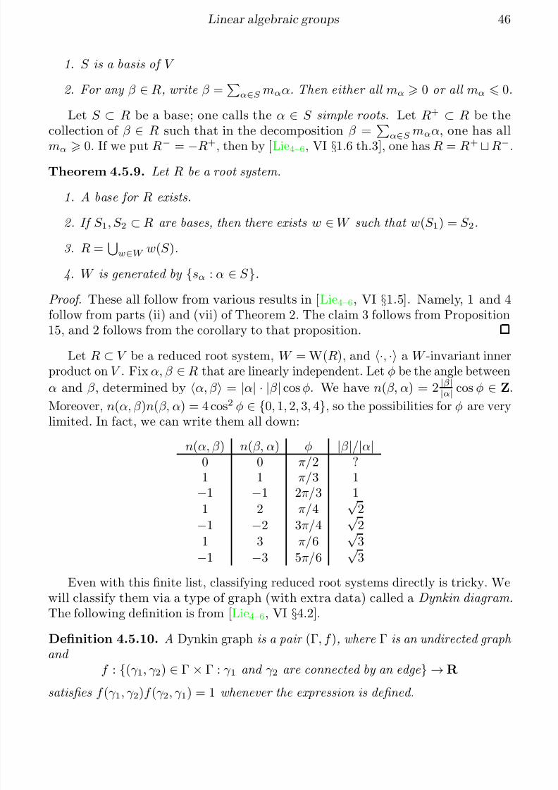
7/18/2019 Linear algebraic groups and their Lie algebras
http://slidepdf.com/reader/full/linear-algebraic-groups-and-their-lie-algebras 46/81
Linear algebraic groups 46
1. S is a basis of V
2. For any β ∈ R, write β =
α∈S mαα. Then either all mα 0 or all mα 0.
Let S ⊂ R be a base; one calls the α ∈ S simple roots . Let R+ ⊂ R be thecollection of β
∈ R such that in the decomposition β = α∈S
mα
α, one has allmα 0. If we put R− = −R+, then by [Lie4–6, VI §1.6 th.3], one has R = R+ R−.
Theorem 4.5.9. Let R be a root system.
1. A base for R exists.
2. If S 1, S 2 ⊂ R are bases, then there exists w ∈ W such that w(S 1) = S 2.
3. R =
w∈W w(S ).
4. W is generated by {sα : α ∈ S }.
Proof. These all follow from various results in [Lie4–6, VI §1.5]. Namely, 1 and 4follow from parts (ii) and (vii) of Theorem 2. The claim 3 follows from Proposition15, and 2 follows from the corollary to that proposition.
Let R ⊂ V be a reduced root system, W = W(R), and ·, · a W -invariant innerproduct on V . Fix α, β ∈ R that are linearly independent. Let φ be the angle between
α and β , determined by α, β = |α| · |β | cos φ. We have n(β, α) = 2 |β||α| cos φ ∈ Z.
Moreover, n(α, β )n(β, α) = 4 cos2 φ ∈ {
0, 1, 2, 3, 4}
, so the possibilities for φ are verylimited. In fact, we can write them all down:
n(α, β ) n(β, α) φ |β |/|α|0 0 π/2 ?1 1 π/3 1
−1 −1 2π/3 1
1 2 π/4√
2−1 −2 3π/4
√ 2
1 3 π/6√
3
−1 −3 5π/6 √ 3Even with this finite list, classifying reduced root systems directly is tricky. We
will classify them via a type of graph (with extra data) called a Dynkin diagram .The following definition is from [Lie4–6, VI §4.2].
Definition 4.5.10. A Dynkin graph is a pair (Γ, f ), where Γ is an undirected graph and
f : {(γ 1, γ 2) ∈ Γ × Γ : γ 1 and γ 2 are connected by an edge } → R
satisfies f (γ 1, γ 2)f (γ 2, γ 1) = 1 whenever the expression is defined.
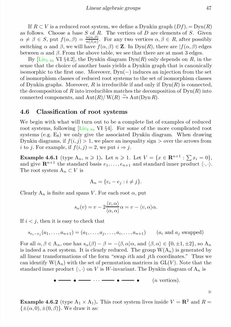
7/18/2019 Linear algebraic groups and their Lie algebras
http://slidepdf.com/reader/full/linear-algebraic-groups-and-their-lie-algebras 47/81
Linear algebraic groups 47
If R ⊂ V is a reduced root system, we define a Dynkin graph (Df ), = Dyn(R)as follows. Choose a base S of R. The vertices of D are elements of S . Givenα = β ∈ S , put f (α, β ) = n(α,β)
n(β,α) . For any two vertices α, β ∈ R, after possibly
switching α and β , we will have f (α, β ) ∈ Z. In Dyn(R), there are |f (α, β ) edgesbetween α and β . From the above table, we see that there are at most 3 edges.
By [Lie4–6, VI §4.2], the Dynkin diagram Dyn(R) only depends on R, in thesense that the choice of another basis yields a Dynkin graph that is canonicallyisomorphic to the first one. Moreover, Dyn(−) induces an injection from the setof isomorphism classes of reduced root systems to the set of isomorphism classesof Dynkin graphs. Moreover, R is irreducible if and only if Dyn(R) is connected,the decomposition of R into irreducibles matches the decomposition of Dyn(R) intoconnected components, and Aut(R)/ W(R)
∼−→ Aut(Dyn R).
4.6 Classification of root systemsWe begin with what will turn out to be a complete list of examples of reducedroot systems, following [Lie4–6, VI §4]. For some of the more complicated rootsystems (e.g. E8) we only give the associated Dynkin diagram. When drawingDynkin diagrams, if f (i, j) > 1, we place an inequality sign > over the arrows fromi to j. For example, if f (i, j) = 2, we put i ⇒ j .
Example 4.6.1 (type An, n 1). Let n 1. Let V = {x ∈ Rn+1 :
xi = 0},and give Rn+1 the standard basis e1, . . . , en+1 and standard inner product ·, ·.
The root system An ⊂ V is
An = {ei − ej : i = j}.
Clearly An is finite and spans V . For each root α, put
sα(v) = v − 2v, αα, αα = v − v, αα.
If i < j, then it is easy to check that
sei−ej (a1, . . . , an+1) = (a1, . . . , aj , . . . , ai, . . . , an+1) (ai and aj swapped)
For all α, β ∈ An, one has sα(β ) − β = −β, αα, and β, α ∈ {0, ±1, ±2}, so An
is indeed a root system. It is clearly reduced. The group W(An) is generated byall linear transformations of the form “swap ith and jth coordinates.” Thus wecan identify W(An) with the set of permutation matrices in GL(V ). Note that thestandard inner product ·, · on V is W -invariant. The Dynkin diagram of An is
• • · · · • • (n vertices).
Example 4.6.2 (type A1 × A1). This root system lives inside V = R2 and R ={±(α, 0), ±(0, β )}. We draw it as:
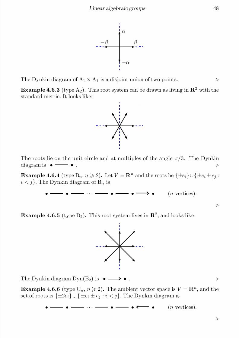
7/18/2019 Linear algebraic groups and their Lie algebras
http://slidepdf.com/reader/full/linear-algebraic-groups-and-their-lie-algebras 48/81
Linear algebraic groups 48
α
−α
β −β
The Dynkin diagram of A1 × A1 is a disjoint union of two points.
Example 4.6.3 (type A2). This root system can be drawn as living in R2 with thestandard metric. It looks like:
The roots lie on the unit circle and at multiples of the angle π/3. The Dynkindiagram is • • .
Example 4.6.4 (type Bn, n 2). Let V = R
n
and the roots be {±ei}∪{±ei± ej :i < j}. The Dynkin diagram of Bn is
• • · · · • • • (n vertices).
Example 4.6.5 (type B2). This root system lives in R2, and looks like
The Dynkin diagram Dyn(B2) is • • .
Example 4.6.6 (type Cn, n 2). The ambient vector space is V = Rn, and the
set of roots is {±2ei}∪{±ei ± ej : i < j}. The Dynkin diagram is
• • · · · • • • (n vertices).
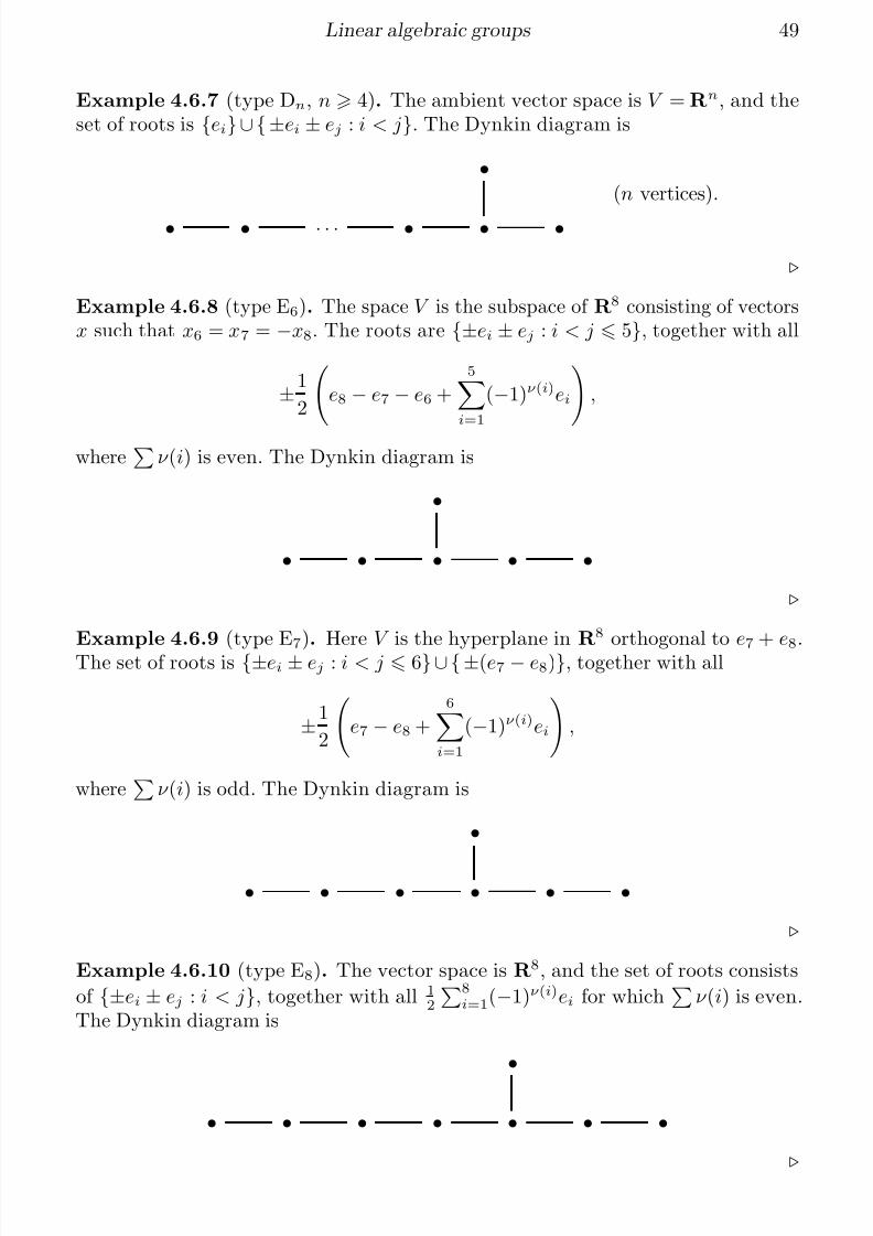
7/18/2019 Linear algebraic groups and their Lie algebras
http://slidepdf.com/reader/full/linear-algebraic-groups-and-their-lie-algebras 49/81
Linear algebraic groups 49
Example 4.6.7 (type Dn, n 4). The ambient vector space is V = Rn, and theset of roots is {ei}∪{±ei ± ej : i < j}. The Dynkin diagram is
•
• • · · · • • •(n vertices).
Example 4.6.8 (type E6). The space V is the subspace of R8 consisting of vectorsx such that x6 = x7 = −x8. The roots are {±ei ± ej : i < j 5}, together with all
±1
2
e8 − e7 − e6 +
5
i=1
(−1)ν (i)ei
,
where
ν (i) is even. The Dynkin diagram is
•
• • • • •
Example 4.6.9 (type E7
). Here V is the hyperplane in R8 orthogonal to e7
+ e8
.The set of roots is {±ei ± ej : i < j 6}∪{±(e7 − e8)}, together with all
±1
2
e7 − e8 +
6i=1
(−1)ν (i)ei
,
where
ν (i) is odd. The Dynkin diagram is
•
• • • • • •
Example 4.6.10 (type E8). The vector space is R8, and the set of roots consists
of {±ei ± ej : i < j}, together with all 12
8i=1(−1)ν (i)ei for which
ν (i) is even.
The Dynkin diagram is
•• • • • • • •
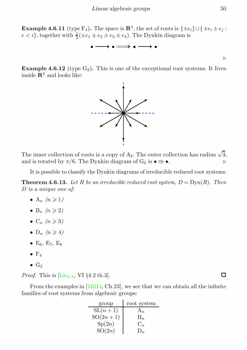
7/18/2019 Linear algebraic groups and their Lie algebras
http://slidepdf.com/reader/full/linear-algebraic-groups-and-their-lie-algebras 50/81
Linear algebraic groups 50
Example 4.6.11 (type F4). The space is R4, the set of roots is {±ei}∪{±ei ± ej :e < i}, together with 1
2 (±e1 ± e2 ± e3 ± e4). The Dynkin diagram is
• • • •
Example 4.6.12 (type G2). This is one of the exceptional root systems. It livesinside R2 and looks like:
The inner collection of roots is a copy of A2. The outer collection has radius√
3,and is rotated by π/6. The Dynkin diagram of G2 is • •.
It is possible to classify the Dynkin diagrams of irreducible reduced root systems.
Theorem 4.6.13. Let R be an irreducible reduced root system, D = Dyn(R). Then D is a unique one of:
• An ( n 1)
• Bn ( n 2)
• Cn ( n 3)
• Dn ( n 4)
• E6, E7, E8
• F4
• G2
Proof. This is [Lie4–6, VI §4.2 th.3].
From the examples in [Mil14, Ch.23], we see that we can obtain all the infinitefamilies of root systems from algebraic groups:
group root systemSL(n + 1) An
SO(2n + 1) Bn
Sp(2n) Cn
SO(2n) Dn
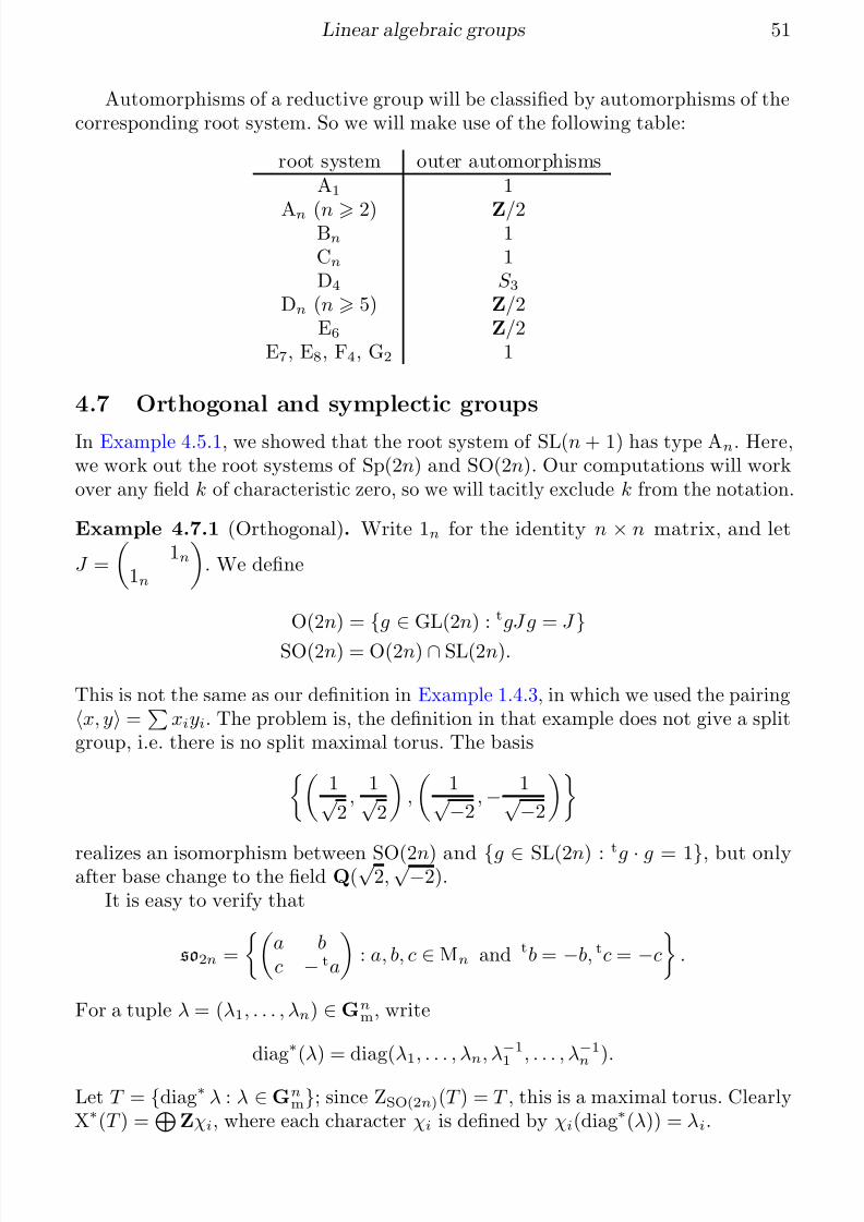
7/18/2019 Linear algebraic groups and their Lie algebras
http://slidepdf.com/reader/full/linear-algebraic-groups-and-their-lie-algebras 51/81
Linear algebraic groups 51
Automorphisms of a reductive group will be classified by automorphisms of thecorresponding root system. So we will make use of the following table:
root system outer automorphismsA1 1
An (n 2) Z/2Bn 1Cn 1D4 S 3
Dn (n 5) Z/2E6 Z/2
E7, E8, F4, G2 1
4.7 Orthogonal and symplectic groups
In Example 4.5.1, we showed that the root system of SL(n + 1) has type An. Here,we work out the root systems of Sp(2n) and SO(2n). Our computations will workover any field k of characteristic zero, so we will tacitly exclude k from the notation.
Example 4.7.1 (Orthogonal). Write 1n for the identity n × n matrix, and let
J =
1n
1n
. We define
O(2n) =
{g
∈ GL(2n) : tgJ g = J
}SO(2n) = O(2n) ∩ SL(2n).
This is not the same as our definition in Example 1.4.3, in which we used the pairingx, y =
xiyi. The problem is, the definition in that example does not give a split
group, i.e. there is no split maximal torus. The basis 1√
2,
1√ 2
,
1√ −2
, − 1√ −2
realizes an isomorphism between SO(2n) and {g ∈ SL(2n) : t
g · g = 1}, but onlyafter base change to the field Q(
√ 2,
√ −2).It is easy to verify that
so2n =
a bc − ta
: a, b, c ∈ Mn and tb = −b, tc = −c
.
For a tuple λ = (λ1, . . . , λn) ∈ Gnm, write
diag∗(λ) = diag(λ1, . . . , λn, λ−11 , . . . , λ−1
n ).
Let T = {diag∗ λ : λ ∈ Gnm}; since ZSO(2n)(T ) = T , this is a maximal torus. Clearly
X∗(T ) =
Zχi, where each character χi is defined by χi(diag∗(λ)) = λi.
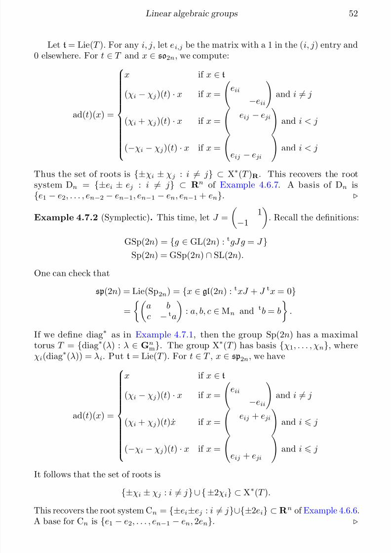
7/18/2019 Linear algebraic groups and their Lie algebras
http://slidepdf.com/reader/full/linear-algebraic-groups-and-their-lie-algebras 52/81
Linear algebraic groups 52
Let t = Lie(T ). For any i, j, let ei,j be the matrix with a 1 in the (i, j) entry and0 elsewhere. For t ∈ T and x ∈ so2n, we compute:
ad(t)(x) =
x if x ∈ t
(χi − χj)(t) · x if x = eii
−eii and i = j
(χi + χj)(t) · x if x =
eij − eji
and i < j
(−χi − χj)(t) · x if x =
eij − eji
and i < j
Thus the set of roots is {±χi ± χj : i = j} ⊂ X∗(T )R. This recovers the rootsystem Dn =
{±ei
± ej : i
= j
} ⊂ Rn of Example 4.6.7. A basis of Dn is
{e1 − e2, . . . , en−2 − en−1, en−1 − en, en−1 + en}.
Example 4.7.2 (Symplectic). This time, let J =
1
−1
. Recall the definitions:
GSp(2n) = {g ∈ GL(2n) : tgJ g = J }Sp(2n) = GSp(2n) ∩ SL(2n).
One can check that
sp(2n) = Lie(Sp2n) = {x ∈ gl(2n) : txJ + J tx = 0}=
a bc − ta
: a, b, c ∈ Mn and tb = b
.
If we define diag∗ as in Example 4.7.1, then the group Sp(2n) has a maximaltorus T = {diag∗(λ) : λ ∈ Gn
m}. The group X∗(T ) has basis {χ1, . . . , χn}, whereχi(diag∗(λ)) = λi. Put t = Lie(T ). For t ∈ T , x ∈ sp2n, we have
ad(t)(x) =
x if x ∈ t
(χi − χj)(t) · x if x = eii
−eii
and i = j
(χi + χj)(t)x if x =
eij + eji
and i j
(−χi − χj)(t) · x if x =
eij + eji
and i j
It follows that the set of roots is
{±χi ± χj : i = j}∪{±2χi} ⊂ X∗(T ).
This recovers the root system Cn = {±ei±ej : i = j}∪{±2ei} ⊂ Rn of Example 4.6.6.A base for Cn is {e1 − e2, . . . , en−1 − en, 2en}.
7/18/2019 Linear algebraic groups and their Lie algebras
http://slidepdf.com/reader/full/linear-algebraic-groups-and-their-lie-algebras 53/81
Linear algebraic groups 53
Both SO(2n) and Sp(2n) are special cases of a more general construction thatstarts with an arbitrary algebra with involution. We follow [Ber10, VIII.21]. Let kbe an arbitrary field of characteristic not 2. An algebra with involution over k is a(possibly non-commutative) k-algebra R together with an anti-involution σ : R → R.The main examples are R = M2n(k) and σ(x) = θ txθ−1 for some invertible matrix
θ, especially θ either 1n1n
or 1n−1n
.
Let (R, σ) be an algebra with involution. The group of similitudes of R is thefunctor Sim(R) from k-algebras to groups, defined by
Sim(R, σ)(A) = {r ∈ (R ⊗k A)× : rσ(r) ∈ A×}.
Similarly, the group of isometries of R is the functor
Iso(R, σ)(A) = {
r ∈
(R⊗k A)× : rσ(r) = 1
}.
Substituting in Mn(k) with an orthogonal or symplectic involution recovers thespecial orthogonal and symplectic groups.
4.8 Classification of split semisimple groups
Let k be a field of characteristic zero. Recall that an algebraic group G/k is said to besplit if there is a maximal torus T ⊂ G which is split. We will use our classificationof root systems to classify split semisimple groups over k.
Definition 4.8.1. A homomorphism f : G → H of algebraic groups is an isogeny if
1. f is surjective, and
2. ker(f ) is finite.
In characteristic p, one has to be very careful, as a lot of nice properties of isogenies fail to hold. For example, in characteristic zero ker(f ) is a finite normalsubgroup of G, hence G acts on ker(f ) by conjugation. If G is connected, this actionmust be trivial, so ker(f )
⊂ Z(G). Thus, in characteristic zero, all isogenies are
central.
Definition 4.8.2. Two semisimple groups G/k, H /k are isogenous if there is a semisimple group J /k with isogenies J G, J H .
It is not obvious, but “being isogenous” is an equivalence relation.
Theorem 4.8.3. Let k be an algebraically closed field of characteristic zero. Then G → R(G, T ) induces a bijection between the set of isogeny classes of connected semisimple groups and isomorphism classes of reduced root systems.
Proof. This follows from [Mil14, 23.14-15].
Unfortunately, we cannot substitute “isomorphism” for “isogeny” in the statementof this theorem.
7/18/2019 Linear algebraic groups and their Lie algebras
http://slidepdf.com/reader/full/linear-algebraic-groups-and-their-lie-algebras 54/81
Linear algebraic groups 54
Example 4.8.4. Work in characteristic zero, and let PGL(n) = GL(n)/ Z(GL(n)).Then PGL(n) and SL(n) have the same root systems. Moreover, the sequence1 → µn → SL(n) → PGL(n) → 1 is exact. So SL(n) and PGL(n) are isogenous butone can check that they are not isomorphic.
The way we have defined “isogenous” as a relation on semisimple groups, it isnot obvious that the relation is transitive. It turns out that the isogeny class of Gcontains two distinguished groups denoted Gad and Gsc. The first, Gad = G/ Z(G)is obviously isogenous to G via the quotient map G Gad. By [Mil14, 21.38],there is also an initial isogeny Gsc → G. One calls Gad the adjoint form of G,and Gsc the simply connected form of G. They (tautologically) fit into a sequenceGsc G Gad of isogenies. So we could have said that two semisimple groups Gand H are isogenous if and only if Gsc H sc.
If we want to classify connected semisimple groups up to isomorphism, we need
a finer invariant than the root system, namely the root datum . We’ll cover root datain more detail in subsection 5.1. For now, all we need is that a root datum can begiven by a reduced root system R ⊂ V together with a group Q(R) ⊂ X ⊂ P (R).Recall that if R ⊂ V , we define
Q(R) = Z · R ⊂ V (root lattice)
P (R) =
x ∈ V :
2x, αα, α ∈ Z for all α ∈ R
(weight lattice).
The letter P for “weight lattice” is possibly inspired by the French word poid for
“weight.”Let G be a semisimple group, T ⊂ G a maximal torus. Let R = R(G, T ) ⊂ X∗(T ).
The inclusion R ⊂ X∗(T )R is a root system. Put X = X∗(T ); then Q(R) ⊂ X ⊂P (R). The quotient group P (R)/Q(R) is finite, so there are only finitely manypossibilities for X .
The group G is simply connected if and only if X = P (R), and adjoint if and onlyif X = Q(R). We already know that each isogeny class has a unique simply connectedsimply connected (resp. adjoint) group. Intermediate quotients Gsc G Gad willcorrespond to quotients of the group πal
1 (Gad) = P (R)/Q(R).
Example 4.8.5. Start with Sp(2n). Let T be as in Example 4.7.2. Recall thatX∗(T ) has basis {χ1, . . . , χn}, where χi(diag∗(λ)) = λi. We showed that the set of roots is
{±χi ± χj : i = j}∪{±2χi} ⊂ X∗(T ).
Now let G = Sp(2n)/{±1}; this contains a maximal torus T /{±1}. Note thatX∗(T / ± 1) → X∗(T ); the image consists of those α ∈ X∗(T ) : α(−1) = 1}. This isZ · R, so Sp(2n)/{±1} = Sp(2n)ad, as we already knew from Z(Sp2n) = µ2. It turnsout that Sp(2n) is simply connected.
The following table is a complete list of the possible isomorphism classes of almost simple algebraic groups over an algebraically closed field of characteristic zero.Recall that an algebraic group is almost simple if its only normal proper subgroupsare finite.
7/18/2019 Linear algebraic groups and their Lie algebras
http://slidepdf.com/reader/full/linear-algebraic-groups-and-their-lie-algebras 55/81
Linear algebraic groups 55
R P/Q Gsc Gad groups in betweenAn (n 1) Z/(n + 1) SLn+1 SLn+1 /µn+1 SLn+1 /µd, d | n + 1Bn (n 2) Z/2 Spin2n+1 SO2n+1
Cn (n 3) Z/2 Sp2n Sp2n /µ2
Dn (n odd) Z/4 Spin2n SO2n /µ2 SO2n
Dn (n even) Z/2 × Z/2 Spin2n SO2n /µ2 SO2n, HSpin2n
G2 1 G2 G2
F4 1 F4 F4
E6 Z/3 (E6)sc (E6)ad
E7 Z/2 (E7)sc (E7)ad
E8 1 E8 E8
Let G be a simply connected semisimple group over k. Then G
Gi, where
each Gi is simply connected and almost simple. Each of the Gi will be one of:
SL(n + 1), Spin(n), Sp(2n), G2, F4, (E6)sc, (E7)sc, E8.
Here, we call an algebraic group G almost simple if all closed normal subgroups N are either trivial (in the sense that N = 1 or N = G) or finite. Similarly, if G is anadjoint group, then G Gi in which each Gi is a simple adjoint group.
Example 4.8.6. The group G = SL(2) × SL(2) has an (obvious) decompositioninto almost simple factors. We have Z(G) = µ2 × µ2. So the quotients of G are:
G,G/(µ2 × 1), G/(1 × µ2), G/∆(µ2), G/(µ2 × µ2).
The group SL(2)×(SL(2)/µ2) is neither adjoint nor simply connected. Here ∆(µ2) ={(x, x) : x ∈ µ2}. The group G/∆(µ2) does not have a product factorization. Itis (obviously) a quotient of SL(2) × SL(2), but is not directly isomorphic to anyH 1 × H 2 for positive-dimensional H i.
Example 4.8.7. Let A be a finite abelian group. We can write A = Z/d1⊕···⊕Z/dn.Then GA = SL(d1) × · · · × SL(dn) has Z(GA) A. So all finite abelian groups ariseas centers of semisimple algebraic groups.
5 Reductive groups
Let k be an algebraically closed field of characteristic zero. Let G/k be a reductivegroup, i.e. RuG = 1. A good example is GL(n). We could like to determine Gup to isomorphism via some combinatorial data. Let T ⊂ G be a maximal torus.Better, let G/k be a split reductive group and k arbitrary of characteristic zero. LetX = X∗(T ). We have the adjoint representation ad : G
→ GL(g). Just as before,
we can writeg = g0 ⊕
α∈R
gα,
where gα = {x ∈ g : tx = α(t)x for all t} and R = {α ∈ X 0 : gα = 0}.
7/18/2019 Linear algebraic groups and their Lie algebras
http://slidepdf.com/reader/full/linear-algebraic-groups-and-their-lie-algebras 56/81
Linear algebraic groups 56
Note that R ⊂ X R need not be a root system, since R may only span a propersubspace of X R. For example, if G is itself a torus, then R = ∅. However,R ⊂ V ⊂ X R, where V = R · R, is a root system, and it determines the semisimplegroup G/RG up to isogeny. The datum “R ⊂ X ” is not in general enough todetermine G.
Let X∗(T ) = hom(Gm, T ). There is a perfect pairing (composition) X∗(T ) ×X∗(T ) → Z = hom(Gm, Gm). Here α, β is the integer n such that α ◦ β is(−)n. From G we’ll construct a root datum, which will be an ordered quadruple(X∗(T ), R(G, T ), X∗(T ), R(G, T )). Before doing this, we’ll define root data in general.
5.1 Root data
The following definitions are from [SGA 3III , XXI]. A dual pair is an ordered pair(X, X ), where X and X are finitely generated free abelian groups, together with a
pairing ·, · : X × X → Z that induces an isomorphism X X ∨ = hom(X, Z). Let(X, X ) be a dual pair, and suppose we have two elements α ∈ X , α ∈ X . Define thereflections sα and sα by
sα(x) = x − x, αα
sα(x) = x − α, xα.
Definition 5.1.1. A root datum consists of an ordered quadruple (X,R, X, R),such that
• (X, X ) is a dual pair.
• R ⊂ X and R ⊂ X are finite sets,
• There is a specified mapping α → α from R to R.
These data are required to satisfy the following conditions:
1. For each α ∈ R, α, α = 2.
2. For each α ∈
R, sα(R) ⊂
R and sα( R) ⊂
R.
It turns out that α → α is a bijection, and that R and R are closed undernegation. If R = (X,R, X, R) is a root datum, the Weyl group of R is the groupW( R ) ⊂ GL(X ) generated by {sα : α ∈ R}. By [SGA 3III , XXI 1.2.8], the Weylgroup of a root datum is finite.
Definition 5.1.2. Let R 1 = (X 1, R1, X 1, R1) and R 2 = (X 2, R2, X 2, R2) be root data. A morphism f : R 1 → R 2 consists of a linear map f : X 1 → X 2 such that
1. f induces a bijection R1∼
−→ R2,
2. The dual map f ∨ : X 2 → X 1 induces a bijection R2∼−→ R1.
Definition 5.1.3. Let R = (X,R, X, R) be a root datum. We say R is reduced if for any α ∈ R, the only multiples of α in R are ±α.
7/18/2019 Linear algebraic groups and their Lie algebras
http://slidepdf.com/reader/full/linear-algebraic-groups-and-their-lie-algebras 57/81
Linear algebraic groups 57
Just as with root systems, there is a notion of a base for root data. If N ⊂ Q
and S ⊂ X , we write N · S for the subset of X Q generated as a monoid by{ns : (n, s) ∈ N × S }. We call a root α ∈ R indivisible if there does not exist anyβ ∈ R for which α = nβ for some n > 1, i.e. Q+ · α ∩ R = {α}.
Definition 5.1.4. Let R = (X,R, X, R) be a root system. A subset ∆ ⊂ R is a base if it satisfies any of the following conditions (reproduced from [ SGA 3 III , XXI 3.1.5]):
1. All α ∈ ∆ are indivisible, and R ⊂ Q+ · ∆ ∪ Q− · ∆.
2. The set ∆ is linearly independent, and R ⊂ N · ∆ ∪ Z− · ∆.
3. Each α ∈ R can be written uniquely as
β∈R mββ , where all mβ ∈ Z and have the same sign.
If ∆ ⊂ R is a base, write R+ = N ·∆ for the set of positive roots and R− = Z− ·∆for the set of negative roots . One has R = R+ R−, and R− = −R+.
Write RtDt for the category of root data. There is a contravariant functor· : RtDt → RtDt which sends a root datum R = (X,R, X, R) to ˇ R = ( X, R,X,R).This is clearly an anti-equivalence of categories. We will use this later to define thedual of a split reductive group. If G/k is a split reductive group, then G will be asplit reductive group scheme over Z, whose root datum is R (G, T )∨.
We’ll write RtDtred for the category of reduced root data.
Example 5.1.5. Let R ⊂ V be a root system. As in subsection 4.8, we havelattices Q(R) ⊂ V (R) ⊂ V . Choose a W -invariant inner product ·, · on V . GivenQ ⊂ X ⊂ P , we can define a root datum as follows:
X = X
R = R
X = {v ∈ V : α, v ∈ Z for all α ∈ R}
R = 2α
α, α
: α
∈ R .
It is easy to check that this satisfies the required properties.
For a classification of “reduced simply connected root systems,” see [SGA 3III ,XXI 7.4.6].
5.2 Classification of reductive groups
Let k be a field of characteristic zero, G/k a (connected) split reductive group. Let
T ⊂ G be a split maximal torus. The rank of G is the integer r = rk(G) = dim(T ).Let g = Lie(G). As we have seen many times before, we can decompose g as arepresentation of T :
g = t ⊕α∈R
gα,
7/18/2019 Linear algebraic groups and their Lie algebras
http://slidepdf.com/reader/full/linear-algebraic-groups-and-their-lie-algebras 58/81
Linear algebraic groups 58
where t = Lie(T ), R = R(G, T ) is the set of roots of G, and gα is the α-typicalcomponent of g. Recall that the Weyl group of G is W(G, T ) = NG(T )/ CG(T ). By[SGA 3II, XII 2.1], the Weyl group is finite.
A good source for what follows is [Jan03, II.1]. Let α : T → Gm be a root,and put T α = (ker α)◦; this is a closed (r
− 1)-dimensional subgroup of T . Let
Gα = CG(T α); by Theorem 4.4.8, this is reductive. One has Z(Gα)◦ = T α. Fromthe embedding Gα → G, we get an embedding of Lie algebras Lie(Gα) → g. By[SGA 3III , IX 3.5], one has
Lie(Gα) = t ⊕ gα ⊕ g−α
and gα, g−α are both one-dimensional. In classical Lie theory, we could defineU α = exp(gα). Since the exponential map does not make sense in full generality, weneed the following result. Recall that we interpret the Lie algebra of an algebraic
group as a new algebraic group.Theorem 5.2.1. Let T act on G via conjugation. Then there is a unique T -equivariant closed immersion uα : gα → G which is also a group homomorphism.
Proof. This is [SGA 3III , XXII 1.1.i].
We let U α be the image of uα. Since gα is one-dimensional, it is isomorphic toGa as a group scheme. So we will generally write uα : Ga
∼−→ U α ⊂ G. The factthat uα is T -equivariant comes down to:
tuα(x)t−1 = uα(α(t)x) t ∈ T , x ∈ Ga.
The group Gα is generated by T , U ±α by Lie algebra considerations. So the groupG is generated by T and {U α : α ∈ R}.
Example 5.2.2 (type An). Inside SL(n + 1), the maximal torus T consists of diagonal matrices diag(t) = diag(t1, . . . , tn+1) for which t1 · · · tn+1 = 1. The groupX∗(T ) is generated by the characters χi(diag(t)) = ti. The roots are {χi−χj : i = j}.For such a root, one can verify that Gα = CG(T α) consists of matrices of the form(gab) for which gab = δ ab unless a = b = i, a = b = j, or (a, b) = (i, j). So
Gα SL(2). It follows that U α = 1 + Gaeij . Note that indeed, SL(n + 1) isgenerated by {U α : α ∈ R} and T .
Back to our general setup T ⊂ Gα ⊂ G. We can consider the “small Weylgroup” W(Gα, T ) ⊂ W(G, T ). Since rk(Gα/ Z(Gα)◦) = 1, we have W(Gα, T ) = Z/2.Let sα be the unique generator of W(Gα, T ). It is known that W = W(G, T ) isgenerated by {sα : α ∈ R}. The group W acts on X∗(T ). Indeed, if w ∈ W , we havew = n for some n ∈ NG(T ). Define (w · χ)(t) = χ(n−1tn).
Recall that X∗(T ) = hom(Gm, T ). There is a natural pairing X∗(T )×X∗(T ) → Z,
for which α, β is the unique n such that αβ is t → tn
. That is, α(β (t)) = tα,β
.This pairing induces an isomorphism X∗(T ) X∗(T )∨.
Theorem 5.2.3. Let α ∈ R. Then there exists a unique α ∈ X∗(T ) such that sα(x) = x − x, αα for all x ∈ X∗(T ). Moreover, α, α = 2.
7/18/2019 Linear algebraic groups and their Lie algebras
http://slidepdf.com/reader/full/linear-algebraic-groups-and-their-lie-algebras 59/81
Linear algebraic groups 59
Proof. This is [SGA 3III , XXII 1.1.ii].
Equivalently, sα(α) = −α. We put R(G, T ) = {α : α ∈ R}. The quadruple
R (G, T ) = (X∗(T ), R(G, T ), X∗(T ), R(G, T ))
is the root datum of G; it will determine G up to isomorphism (not just isogeny).In defining coroots, we could also have used the fact that Z(Gα)◦ = T α, which
implies T /T α → Gα/T α is a maximal torus of dimension 1. So the group Gα/T α issemisimple, and has one-dimensional maximal torus. Its Dynkin diagram has typeA1, so Gα/T α is either SL(2) or PGL(2).
Definition 5.2.4. Let k be a field, G/k a split reductive group. A pinning of Gconsists of the following data:
1. A maximal torus T ⊂ G.2. An isomorphism T
∼−→ D(M ) for some free abelian group M .
3. A base ∆ ⊂ R(G, T ).
4. For each α ∈ ∆, a non-zero element X α ∈ gα.
If G1, G2 are pinned reductive groups, a morphism f : G1 → G2 is said to becompatible with the pinnings if f (T 1) = f (T 2), f induces a bijection (written f ∗)R1
∼
−→ R2, and such that
f (uα(X 1,α)) = uf ∗α(X 2,f ∗α).
Let RdGppinn/k be the category of split reductive groups over k with pinnings. We
can define a pinning of a root system R = (X,R, X, R) to be the choice of a base∆ ⊂ R. Let RtDtred,pinn be the category of pinned reduced root data. The followingcombines the “existence and uniqueness theorems” in the classification of reductivegroups.
Theorem 5.2.5. The operation G → R (G, T ) induces an equivalence of categories
RdGppinn/k
∼−→ RtDtred,pinn.
Proof. See [SGA 3III , XXIII 4.1] for a proof that R is fully faithful, [SGA 3III , XXV2] for a proof of essential surjectivity.
5.3 Chevalley-Demazure group schemes
In Theorem 5.2.5, we classified split reductive groups over an arbitrary field. It turnsout that the classification works over an arbitrary (non-empty) base scheme. Moreprecisely, let S be a scheme, G/S a smooth affine group scheme of finite type. Wesay G is reductive if each geometric fiber Gs is reductive. A maximal torus in G is asubgroup scheme T ⊂ G of multiplicative type such that for all s ∈ S , the geometric
7/18/2019 Linear algebraic groups and their Lie algebras
http://slidepdf.com/reader/full/linear-algebraic-groups-and-their-lie-algebras 60/81
Linear algebraic groups 60
fiber T s ⊂ Gs is a maximal torus. Suppose there exists an abelian group M with anembedding D(M )/S → G whose image is a maximal torus. Just as before, there isa decomposition g = t ⊕ gα, except now g (and the gα) is a locally free sheaf onS . We say that G is split if the following conditions hold:
1. Each gα is a free O S -module.
2. Each root α (resp. each coroot α) is constant, i.e. induced by an element of M (resp. M ∨).
Given the obvious notion of “pinned reductive group over S ,” the classification resultin Theorem 5.2.5 actually gives an equivalence of categories
RdGppinn/S
∼−→ RtDtred,pinn.
In particular, for each reduced root datum R , there is a reductive group scheme GR/Z
with root datum R , such that for any scheme S , the unique (up to isomorphism)reductive group scheme with root datum R is the base-change GR/S = (GR/Z)S .In particular, if k is a field, the unique split reductive k-group with root datum R isGR/k. One calls GR/Z the Chevalley-Demazure group scheme of type R .
6 Special topics
6.1 Borel-Weil theorem
1
Let k be a field of characteristic zero, G/k an algebraic group. We write Mod(G)for the category whose objects are (not necessarily finite-dimensional) vector spacesV together with ρ : G → GL(V ). Here, GL(V ) is the fppf sheaf (not representableunless V is finite-dimensional) S → GL(V O (S )). The action action of G on itself bymultiplication induces an action of G on the (k-vector spaces) O (G), which is notfinite-dimensional unless G is finite. By [Jan03, I 3.9], the category Mod(G) hasenough injectives; this enables us to define derived functors in the usual way.
Let H
⊂ G be an algebraic subgroup. There is an obvious functor resGH :
Mod(G) → Mod(H ) which sends (V, ρ : G → GL(V )) to (V, ρ|H ). It has a rightadjoint, the induction functor , determined by
homG(V, indGH U ) = homH (resGH V, U ).
We are especially interested in this when U is finite-dimensional, in which case wehave
indGH U = {f : G → V(U ) : f (gh) = h−1f (g) for all g ∈ G}.
Since the induction functor is a right adjoint, it is left-exact, so it makes sense to
talk about its derived functors R• indGH . It turns out that these can be computedas the sheaf cohomology of certain locally free sheaves on the quotient G/H . Let
1Balazs Elek
7/18/2019 Linear algebraic groups and their Lie algebras
http://slidepdf.com/reader/full/linear-algebraic-groups-and-their-lie-algebras 61/81
Linear algebraic groups 61
π : G G/H be the quotient map; for a representation V of H , define an O G/H -module L (V ) by
L (V )(U ) = (V ⊗ O (π−1U ))G.
By [Jan03, I 5.9], the functor L (−) is exact, and sends finite-dimensional repre-
sentations of H to coherent O
G/H -modules. Moreover, by [Jan03, I 5.12] there is acanonical isomorphism
R• indGH V = H•(G/H,L (V )). (∗)
In general, both the vector spaces in (∗) will not be finite-dimensional. However,if G/H is proper, then finiteness theorems for proper pushforward [EGA 3I, 3.2.1]tell us that H•(G/H,F ) is finite-dimensional whenever F is coherent. So we can useRi indGH to produce finite-dimensional representations of G from finite-dimensionalrepresentations of H .
Note : for the remainder of this section, “representation” means finite-dimensional representation, while “module” means possibly infinite-dimensional representation.
Let G/k be a split reductive group, B ⊂ G a Borel subgroup and T ⊂ B amaximal torus. Let N = RuB; one has B T N . In particular, we can extendχ ∈ X∗(T ) to a one-dimensional representation of B by putting χ(tn) = χ(t) fort ∈ T , n ∈ N .
Theorem 6.1.1. Every irreducible representation of G is a quotient of indGB χ for a unique χ
∈ X∗(T ).
Proof. Let V be an irreducible representation of G. The group B acts on theprojective variety P(V ); by 4.1.5 there is a fixed point v, i.e. resGB V containsa one-dimensional subrepresentation. This corresponds to a B-equivariant mapχ → resGB V for some χ ∈ X∗(T ). By the definition of induction functors, we get a
nonzero map indGB χ → V . Since V is simple, it must be surjective. Uniqueness of χis a bit trickier.
One calls χ the highest weight of V . A natural question is: for which χ isindGB χ irreducible? By [Jan03, II 2.3], indGB χ (if nonzero) contains a unique simplesubrepresentation, which we denote by L(χ).
Recall that our choice of Borel B ⊂ T induces a base S ⊂ R(G, T ) ⊂ X∗(T ).We put an ordering on X∗(T ) by saying that λ µ if µ − λ ∈ N · S . It is knownthat there exists w0 ∈ W = W(G, T ) such that w0(R+) = R−. Finally, the set of dominant weights is:
X∗(T )+ = {χ ∈ X∗(T ) : χ, α 0 for all α ∈ R+}.
We can now classify irreducible representations of G.
Theorem 6.1.2. Any irreducible representation of G is of the form L(χ) for a unique χ ∈ X∗(T )+.
Proof. This is [Jan03, II 2.7].
7/18/2019 Linear algebraic groups and their Lie algebras
http://slidepdf.com/reader/full/linear-algebraic-groups-and-their-lie-algebras 62/81
Linear algebraic groups 62
The Borel-Weil theorem completely describes R• indGB(χ) for dominant χ. Firstwe need some definitions. If w ∈ W , the length of w, denoted l(w), is the minimal nsuch that w can be written as a product s1 · · · sn of simple reflections. Let S be aset of simple roots, ρ = 1
2
α∈R+ α. The “dot action” of W on character is:
w • χ = w(χ + ρ) − ρ.
DefineC = {χ ∈ X∗(T ) : χ + ρ, α for all α ∈ R+}.
It turns out that all χ ∈ X∗(T ) are of the form w • χ1 for some χ1 ∈ C . Thus thefollowing theorem describes R• indGB χ for all χ.
Theorem 6.1.3 (Borel-Weil). Let χ ∈ C . If c /∈ X∗(T )+, then R• indGB(w • χ) = 0 for all w ∈ W . If χ ∈ X∗(T )+, then for all w ∈ W ,
Ri indGB(w • χ) =L(χ) i = l(w)
0 otherwise
Proof. This is [Jan03, II 5.5].
Putting w = 1, we see that indGB(χ) = L(χ).
6.2 Tannakian categories
Throughout, k is an arbitrary field of characteristic zero. We will work over k, soall maps are tacitly assumed to be k-linear and all tensor product will be over k.Consider the following categories.
For G/k an algebraic group, the category Rep(G) has as objects pairs (V, ρ), whereV is a finite-dimensional k-vector space and ρ : G → GL(V ) is a homomorphism of k-groups. A morphism (V 1, ρ1) → (V 2, ρ2) in Rep(G) is a k-linear map f : V 1 → V 2such that for all k-algebras A and g ∈ G(A), one has f ρ1(g) = ρ2(g)f , i.e. thefollowing diagram commutes:
V 1 ⊗ A V 2 ⊗ A
V 1 ⊗ A V 2 ⊗ A.
f
ρ1(g) ρ2(g)
f
Example 6.2.1 (Representations of a Hopf algebra). Let H be a co-commutativeHopf algebra. The category Rep(H ) has as objects H -modules that are finite-dimensional over k, and morphisms are k-linear maps. The algebra H acts on atensor product U ⊗ V via its comultiplication ∆ : H → H ⊗ H .
Example 6.2.2 (Representations of a Lie algebra). Let g be a Lie algebra over k.The category Rep(g) has as objects g-representations that are finite-dimensional asa k-vector space. There is a canonical isomorphism Rep(g) = Rep( U g), where U g isthe universal enveloping algebra of g.
7/18/2019 Linear algebraic groups and their Lie algebras
http://slidepdf.com/reader/full/linear-algebraic-groups-and-their-lie-algebras 63/81
Linear algebraic groups 63
Example 6.2.3 (Continuous representations of a compact Lie group). Let K be acompact Lie group. The category RepC(K ) has as objects pairs (V, ρ), where V is afinite-dimensional complex vector space and ρ : K → GL(V ) is a continuous (hencesmooth, by Cartan’s theorem) homomorphism. Morphisms (V 1, ρ1) → (V 2, ρ2) areK -equivariant C-linear maps V 1
→ V 2.
Example 6.2.4 (Graded vector spaces). Consider the category whose objects arefinite-dimensional k-vector spaces V together with a direct sum decompositionV =
n∈Z V n. Morphisms U → V are k-linear maps f : U → V such that
f (U n) ⊂ V n.
Example 6.2.5 (Hodge structures). Let V be a finite-dimensional R-vector space.A Hodge structure on V is a direct sum decomposition V C =
V p,q such that
V p,q = V q,p. If U, V are vector spaces with Hodge structures, a morphism U → V isa R-linear map f : U
→ V such that f (U
p,q) ⊂
V p,q
. Write Hdg for the category of vector spaces with Hodge structure.
Let Vect(k) be the category of finite-dimensional k-vector spaces. For C any of the categories above, there is a faithful functor ω : C → Vect(k). In our examples,it is just the forgetful functor. The main theorem will be that for π = Aut(ω), thefunctor ω induces an equivalence of categories C ∼−→ Rep(π). We proceed to makesense of the undefined terms in this theorem.
Our definitions follow [DM82]. As before, k is an arbitrary field of characteristiczero.
Definition 6.2.6. A k-linear category is an abelian category C such that each V 1, V 2,the group hom(V 1, V 2) has the structure of a k-vector space in such a way that the composition map hom(V 2, V 3) ⊗ hom(V 1, V 2) → hom(V 1, V 3) is k-linear. For us, a rigid k-linear tensor category is a k-linear category C together with the following data:
1. An exact faithful functor ω : C → Vect(k).
2. A bi-additive functor
⊗ :
C × C → C.
3. Natural isomorphisms ω(V 1 ⊗ V 2) ∼−→ ω(V 1) ⊗ ω(V 2).
4. Isomorphisms V 1 ⊗ V 2∼−→ V 2 ⊗ V 1 for all V i ∈ C.
5. Isomorphisms (V 1 ⊗ V 2) ⊗ V 3∼−→ V 1 ⊗ (V 2 ⊗ V 3)
These data are required to satisfy the following conditions:
1. There exists an object 1 ∈ C such that ω(1) is one-dimensional and such that the natural map k
→ hom(1, 1) is an isomorphism.
2. If ω(V ) is one-dimensional, there exists V −1 ∈ C such that V ⊗ V −1 1.
3. Under ω, the isomorphisms 3 and 4 are the obvious ones.
7/18/2019 Linear algebraic groups and their Lie algebras
http://slidepdf.com/reader/full/linear-algebraic-groups-and-their-lie-algebras 64/81
Linear algebraic groups 64
By [DM82, Pr. 1.20], this is equivalent to the standard (more abstract) definition.Note that all our examples are rigid k-linear tensor categories. One calls the functorω a fiber functor .
Let (C, ⊗) be a rigid k-linear tensor category. In this setting, define a functorAut(ω) from k-algebras to groups by setting:
Aut⊗(ω)(A) = Aut⊗ (ω : C ⊗ A → Rep(A))
=
(gV ) ∈
V ∈C
GL(ω(V ) ⊗ A) : gV 1⊗V 2 = gV 1 ⊗ gV 2 , andf gV 1 = gV 1f for all f, V 1, V 2
.
In other words, an element of Aut(ω)(A) consists of a collection (gV ) of A-linearautomorphisms gV : ω(V ) ⊗ A
∼−→ ω(V ) ⊗ A, where V ranges over objects in C. Thiscollection must satisfy:
1. g1 = 1ω(1)
2. gV 1⊗V 2 = gV 1 ⊗ gV 2 for all V 1, V 2 ∈ C, and
3. whenever f : V 1 → V 2 is a morphism in C, the following diagram commutes:
ω(V 1)A ω(V 2)A
ω(V 1)A ω(V 2)A.
f
gV 1 gV 2
f
Typically one only considers affine group schemes G/k that are algebraic , i.e. whosecoordinate ring O (G) is a finitely generated k-algebra, or equivalently that admita finite-dimensional faithful representation. Let G/k be an arbitrary affine groupscheme, V an arbitrary representation of G over k. By [DM82, Cor. 2.4], onehas V = lim−→ V i, where V i ranges over the finite-dimensional subrepresentationsof V . Applying this to the regular representation G → GL(O (G)), we see thatO (G) = lim−→O (Gi), where Gi ranges over the algebraic quotients of G. That is,an arbitrary affine group scheme G/k can be written as a filtered projective limit
G = lim←− Gi, where each Gi is an affine algebraic group over k. So we will speak of pro-algebraic groups instead of arbitrary affine group schemes.
If V is a finite-dimensional k-vector space and G = lim←− Gi is a pro-algebraick-group, representations G → GL(V ) factor through some algebraic quotient Gi.That is, hom(G, GL(V )) = lim−→ hom(Gi, GL(V )). As a basic example of this, let Γbe a profinite group, i.e. a projective limit of finite groups. If we think of Γ as apro-algebraic group, then algebraic representations Γ → GL(V ) are exactly thoserepresentations that are continuous when V is given the discrete topology.
First, suppose C = Rep(G) for a pro-algebraic group G, and that ω : Rep(G) →Vect(k) is the forgetful functor. Then the Tannakian fundamental group Aut
⊗
(ω)carries no new information [DM82, Pr. 2.8]:
Theorem 6.2.7. Let G/k be a pro-algebraic group, ω : Rep(G) → Vect(k) the
forgetful functor. Then G ∼−→ Aut⊗(G).
7/18/2019 Linear algebraic groups and their Lie algebras
http://slidepdf.com/reader/full/linear-algebraic-groups-and-their-lie-algebras 65/81
Linear algebraic groups 65
The main theorem is the following, taken essentially verbatum from [DM82,Th. 2.11].
Theorem 6.2.8. Let (C, ⊗, ω) be a rigid k-linear tensor category. Then π = Aut⊗(ω)is represented by a pro-algebraic group, and ω : C → Rep(π) is an equivalence of
categories.Often, the group π1(C) is “too large” to handle directly. For example, if C
contains infinitely many simple objects, probably π1(C) will be infinite-dimensional.For V ∈ C, let C(V ) be the Tannakian subcategory of C generated by V . Oneputs π1(C/V ) = π1(C(V )). It turns out that π1(C/V ) ⊂ GL(ωV ), so π1(C/V ) isfinite-dimensional. One has π1(C) = lim←− π1(C/V ).
Example 6.2.9 (Pro-algebraic groups). If G/k is a pro-algebraic group, thenTheorem 6.2.7 tells us that if ω : Rep(G) → Vect(k) is the forgetful functor, thenG = Aut⊗(G). That is, G = π1(RepG).
Example 6.2.10 (Hopf algebras). Suppose H is a co-commutative Hopf algebraover k. Then π1(RepH ) = Spec(H ◦), where H ◦ is the reduced dual defined in [Car07].Namely, for any k-algebra A, A◦ is the set of k-linear maps λ : A → k such thatλ(a) = 0 for some two-sided ideal a ⊂ A of finite codimension. The key fact here isthat (A ⊗ B)◦ = A◦ ⊗ B◦, so that we can use multiplication m : H ⊗ H → H todefine comultiplication m∗ : H ◦ → (H ⊗ H )◦ = H ◦ ⊗ H ◦. From [DG80, II §6 1.1], if G is a linear algebraic group over an algebraically closed field k of characteristic zero,we get an isomorphism O (G)◦ = k[G(k)] ⊗ U (g). Here k[G(k)] is the usual group
algebra of the abstract group G(k), and U (g) is the universal enveloping algebra of g = Lie(G), both with their standard Hopf structures.
[Note: one often calls O (G)◦ the “space of distributions on G.” If instead G is areal Lie group, then one often writes H (G) for the space of distributions on G. LetK ⊂ G be a maximal compact subgroup, M (K ) the space of finite measures on K .Then convolution D ⊗ µ → D ∗ µ induces an isomorphism U (g) ⊗ M (K )
∼−→ H (G).In the algebraic setting, k[G(k)] is the appropriate replacement for M (K ).]
Example 6.2.11 (Lie algebras). Let g be a semisimple Lie algebra over k. Thenby [Mil07], G = π1(Repg) is the unique connected, simply connected algebraic groupwith Lie(G) = g. If g is not semisimple, e.g. g = k, then things get a lot nastier. Seethe above example.
Example 6.2.12 (Compact Lie groups). By definition, the complexification of areal Lie group K is a complex Lie group K C such that all morphisms K → GL(V )factor uniquely through K C → GL(V ). It turns out that K C is a complex algebraicgroup, and so π1(RepK ) = K C.
Example 6.2.13 (Graded vector spaces). To give a grading V =
n∈Z V n on a
vector space is equivalent to giving an action of the split rank-one torus Gm. On each
V n, Gm acts via the character g → gn. Thus π1(graded vector spaces) = Gm. Example 6.2.14 (Hodge structures). Let S = RC/R Gm; this is defined by S(A) =(A⊗C)× for R-algebras A. One can check that the category Hdg of Hodge structuresis equivalent to RepR(S). Thus π1(Hdg) = S.
7/18/2019 Linear algebraic groups and their Lie algebras
http://slidepdf.com/reader/full/linear-algebraic-groups-and-their-lie-algebras 66/81
Linear algebraic groups 66
6.3 Automorphisms of semisimple Lie algebras2
Let k be a field of characteristic zero, g a split semisimple Lie algebra over k. Wewant to describe the group Aut(g). It turns out Aut(g) = Aut(Gsc), where Gsc isthe unique simply connected semisimple group with Lie algebra g. We can give
Aut(g) the structure of a linear algebraic group by puttingAut(g)(A) = Aut(gA).
Clearly Aut(g) ⊂ GL(g). Let t ⊂ g be a maximal abelian subalgebra. Let R ⊂ t ∨
be the set of roots, S ⊂ R a base of ∆. We can define some subgroups of Aut(g):
Aut(g, t ) = {θ ∈ Aut(g) : θ(t ) = t }Aut(g, t , S ) = {θ ∈ Aut(g, t ) : tθ(S ) = S }.
Lemma 6.3.1. If θ
∈ Aut(g, t ), then tθ(R) = R.
Proof. The definition of R is invariant under automorphisms of t .
Let Aut(R) be the set of automorphisms of the Dynkin diagram associated to R.
Lemma 6.3.2. The natural map ε : Aut(g, t , S ) → Aut(R) is surjective.
Proof. Choose, for each α ∈ R, a non-zero element xα ∈ gα. The existence theorem[Lie7–9, VIII §4.4 th.2] tells us that to each automorphism ϕ of the Dynkin diagramof R, there exists a unique ϕ ∈ Aut(g, t , S, {xα}) inducing ϕ. Thus ε : Aut(t , t , S ) →Aut(R) splits.
We want to describe the kernel of ε. Since g is semisimple, the adjoint mapg → Der(g) = Lie(Aut g) is an embedding, and thus t
∼−→ ad(t ). Let T ⊂ Inn(g) bethe subgroup with Lie algebra ad(t ).
Lemma 6.3.3. ker(ε) = T .
Proof. Clearly T ⊂ ker(ε). Let θ ∈ ker(ε). For any α ∈ R, we have θxα ∈ gβ forsome β . For t ∈ t , we compute:
[t,θxα] = [θt,θxα]
= θ[t, xα]= α(t)θxα,
so α = β . Moreover, θ acts on g exactly like an element of t , so θ ∈ T .
Lemma 6.3.4. Aut(g) = Aut(g, t , S ) · Inn(g).
Proof. Use the well-known facts that all Cartan subalgebras of g are conjugate, andthat moreover the Weyl group acts transitively on sets of simple roots.
We have arrived at the main result.
Theorem 6.3.5. Aut(g) = Inn(g) Aut(R). In particular, Out(g) = Aut(R).
This allows us to recover the table of automorphisms in subsection 4.6.
2Sasha Patotski
7/18/2019 Linear algebraic groups and their Lie algebras
http://slidepdf.com/reader/full/linear-algebraic-groups-and-their-lie-algebras 67/81
Linear algebraic groups 67
6.4 Exceptional isomorphisms3
Terence Tao’s blog post at http://terrytao.wordpress.com/2011/03/11/ is anexcellent reference for this section. From Theorem 4.8.3, we know that the setof isogeny classes of split semisimple algebraic groups is the same as the set of
isomorphism classes of Dynkin diagrams. In Theorem 4.6.13, we classified theDynkin diagrams. In this classification, we just included, e.g. Dn for n 4. If weinclude all the Dn etc., the classification is no longer unique – we have to accountfor the “exceptional isomorphisms”
A1 B1 C1 D2 E1
B2 C2
D3 A3
D2
A1
×A1.
The Dynkin diagram for D2 and A1 × A1 is disconnected – it is a disjoint unionof two points. We’ll explicitly construct the induced isogenies between algebraicgroups of different types.
Example 6.4.1 (A1 C1). Since Sp(2) = SL(2), there is nothing to prove.
Example 6.4.2 (A1 B1). Define a pairing on sl2 by x, y = tr(xy) (the Killing form ). One easily verifies that the adjoint action of SL(2) on sl2 preserves thisform. Moreover, a general theorem of linear algebra tells us that any non-degeneratebilinear symmetric pairing on a three-dimensional vector space is isomorphic tothe orthogonal pairing. It follows that Aut( sl2, ·, ·) O(3), at least over analgebraically closed field. Since SL(2) is connected, ad(SL(2)) ⊃ SO(3). A dimensioncount tells us that SL(2)/µ2 SO(3). Again, this only works over an algebraicallyclosed field.
Example 6.4.3 (D2 A1 × A1). We need to show that SO(4) and SL(2) × SL(2)are isogenous. Let std : SL(2) → GL(2) be the standard representation, and considerthe representation std std of SL(2) × SL(2). There is an obvious bilinear formform:
u1 ⊗ u2, v1 ⊗ v2 = ω(u1, v1)ω(u2, v2),where ω is the determinant pairing k2 × k2 → 2 k2 k given by (x, y) → x ∧ y.The group SL(2) × SL(2) acts on std std by (g, h)(v ⊗ w) = (gv) ⊗ (gw). Thus wehave a representation SL(2) × SL(2) → GL(4). The image preserves ·, ·, hence (bylinear algebra) lies inside O(4), By connectedness and a dimension count, we seethat this is an isogeny SL(2) × SL(2) SO(4).
6.5 Constructing some exceptional groups4
We roughly follow [SV00]. Let k be a field of characteristic not 2 or 3. Recall that if V is a k-vector space and ·, · : V × V → k is a symmetric bilinear form, we can
3Theodore Hui4Gautam Gopal
7/18/2019 Linear algebraic groups and their Lie algebras
http://slidepdf.com/reader/full/linear-algebraic-groups-and-their-lie-algebras 68/81
Linear algebraic groups 68
define a quadratic form q : V → k by q (v) = v, v. This correspondence is bijective;we can go backwards via the familiar identity
u, v = 1
2(q (u + v) − q (u) − q (v)).
Definition 6.5.1. A composition algebra is a pair (C, q ), where C is a unital, not-necessarily associative k-algebra and q is a multiplicative non-degenerate quadratic on C .
In other words, we require q (xy) = q (x)q (y) for all x, y ∈ C . Since by [SV00,1.2.4], q is determined by the multiplicative strucure of C , we will just refer to “acomposition algebra C .” Write e for the unit of C . Every composition algebra comeswith a natural involution x → x, defined by x = x, e − x.
Theorem 6.5.2. Let C be a composition algebra. Then dim(C ) ∈ {1, 2, 4, 8}.Proof. This is [SV00, 1.6.2].
We call an 8-dimensional composition algebra an octobian algebra . If C is anoctonian k-algebra, we define an algebraic group Aut(C ) by putting
Aut(C )(A) = {g ∈ GL(C ⊗ A) : g is a morphism of normed A-algebras},
for all (commutative, unital) k-algebras A. There is an obvious embedding Aut(C ) →O(C, q ).Theorem 6.5.3. Let C be an octonian k-algebra. Then Aut(C ) is a connected algebraic group of type G2.
Proof. We mean that after base-change to an algebraic closure of k, Aut(C ) becomesisomorphic to G2. This is [SV00, 2.3.5].
If C is a composition algebra and γ = (γ 1, γ 2, γ 3) ∈ (k×)3, we define a newalgebra H C,γ to be as a set the collection of matrices
z1 c3 γ −11 γ 3c2
γ −12 γ 1c3 z2 c1
c2 γ −13 γ 2c1 z3
ci ∈ k× and zi ∈ k.
Give H C,γ the product xy = 12 (x · y + y · x) and quadratic form q (x) = 1
2 tr(x2).
Definition 6.5.4. An Albert algebra is a commutative, non-unital, associative k-algebra A such that A ⊗ k is isomorphic to a k-algebra of the form H C,γ for some octobian algebra C and γ
∈ k×.
If A is an Albert algebra, we can define an algebraic group Aut(A) just as above.
Theorem 6.5.5. If A is an Albert algebra, then Aut(A) is a connected simple algebraic group of type F4.
7/18/2019 Linear algebraic groups and their Lie algebras
http://slidepdf.com/reader/full/linear-algebraic-groups-and-their-lie-algebras 69/81
Linear algebraic groups 69
Proof. Put G = Aut(A). Call an element u ∈ A idempotent if u2 = u. It turnsout that if u is idempotent, then either u ∈ {0, e}, or q (u) ∈ {1/2, 1}. Callthe idempotents with q (u) = 1/2 primitive . Let V ⊂ A be the set of primitiveidempotents; this is naturally a variety over k. It turns out that V is 16-dimensionalclosed and irreducible and has a transitive G-action. For some v
∈ V , the group
Gv = StabG(v) is the spin group of a nine-dimensional quadratic form, so dim(Gv) =36. It follows that dim(G) = 16 + 36 = 52. Since Gv and V are irreducible, G isconnected. From the action of G on e⊥ ⊂ A, we see that G is semisimple algebraic.The only 52-dimensional semisimple algebraic group over an algebraically closedfield is F4. For a more careful proof, see [SV00, 7.2.1].
It turns out that any group of type F4 can be obtained as Aut(A) for someAlbert algebra A. Consider the cubic form
det(x) = z1z2z3 − γ
−1
3 γ 2z1q (c1) − γ
−1
2 γ 3z2q (c2) − γ
−1
2 γ 1z3q (c3) + c1c2, c3.
Let GL(A, det) be the subgroup of GL(A) consisting of those linear maps whichpreserve det.
Theorem 6.5.6. Let A be an Albert algebra. Then GL(A, det) is a connected simple algebraic group of type E6.
Proof. This is [SV00, 7.3.2].
Unlike the case with groups of type F4, not all groups of type E6 can be obtainedthis way.
6.6 Spin groups5
The motivation for spin groups is as follows. Recall that up to isogeny, the simplealgebraic groups are SL(n), Sp(2n), SO(n), or one of the exceptional groups. Recallthat each isogeny class has two distinguished elements, the simply connected andadjoint. For SO(n), we should expect there to be a simply connected group Spin(n) =(Dn)sc, which is a double cover of SO(n).
Work over a field k of characteristic not 2. Let V be a k-vector space, q aquadratic form on V . The Clifford algebra Cl(V, q ) is the quotient of the tensoralgebra T (V ) by the ideal generated by {v ⊗ v − q (v) : v ∈ V }. There is an obviousinjection V → Cl(V, q ), and k-linear maps f : V → A into associative k-algebraslift to f : Cl(V, q ) → A if and only if f (v)f (v) = q (v) for all v ∈ V . This univeralproperty clearly characterizes Cl(V, q ). For brevity, write Cl(V ) = Cl(V, q ).
Example 6.6.1. Let V = R4, q be the indefinite form of signature (3, 1), i.e. q (v) =
−v2
1 + v22 + v32 + v2
4 . We write Cl(1,3)(R) for the Clifford algebra Cl(V, q ); it has
presentation
Cl(1,3)(R) = Re1, e2, e3, e4/(e21 = −1, e2
2 = e23 = e2
4 = 1).
5Benjamin ?
7/18/2019 Linear algebraic groups and their Lie algebras
http://slidepdf.com/reader/full/linear-algebraic-groups-and-their-lie-algebras 70/81
Linear algebraic groups 70
This is used in the Dirac equation, which unifies special relativity and quantummechanics.
There is a clear action O(V, q ) → Aut Cl(V ). In particular, the involutionα(v) = −v induces an involution (also denoted α) of Cl(V ). This induces a grading
Cl(V ) = Cl0
(V ) ⊕ Cl1
(V ), where
Cl0(V ) = {x ∈ Cl(V ) : α(x) = x}Cl1(V ) = {x ∈ Cl(V ) : α(x) = −x}.
We define some algebraic groups via their functors of points:
Pin(V, q )(A) = {g ∈ Cl(V, q )A : q (g) ∈ µ2(A)}Spin(V, q ) = Pin(V, q )
∩Cl0(V ).
There is a “twisted adjoint map” ad : Pin(V, q ) → O(V, q ), given by ad(g)(v) =α(g)vg−1.
Theorem 6.6.2. There is a natural exact sequence
1 → µ2 → Spin(V, q ) → SO(V, q ) → 1.
Proof. This is [Ber10, IV.10.21].
6.7 Differential Galois theory6
A good source for differential Galois theory is [PS03]. Recall that if A is a ring,a derivation on A is an additive map ∂ : A → A satisfying the Liebniz rule :∂ (ab) = a∂ (b) + ∂ (a)b. We write Der(A) for the group of derivations A → A.
Definition 6.7.1. A differential ring is a pair (R, ∆), where ∆ ⊂ Der(R) is such that ∂ 1∂ 2 = ∂ 2∂ 1 for all ∂ 1, ∂ 2 ∈ ∆.
If ∆ = {∂ }, we write r
= ∂r for r ∈ R. The ring C = {c ∈ R : ∂c = 0 for all ∂ ∈∆} is called the ring of constants . If R is a field, we call (R, ∆) a differential field .
Example 6.7.2. Let R = C ∞(Rn) and ∆ = { ∂ ∂xi: 1 i n}. Then (R, ∆) is a
differential ring with R as ring of constants.
Example 6.7.3. Let k be a field, R = k(x1, . . . , xn), and ∆ = { ∂ ∂xi: 1 i n}.
Then (R, ∆) is a differential field with field of constants k.
We are interested in solving matrix differential equations , that is, equations of
the form y
= Ay for A ∈ Mn(k). A solution would be a tuple y = (y1, . . . , yn) ∈ k
n
such that (y1, . . . , yn) = Ay. To a matrix differential equation we will associate twoobjects: a Picard-Vessiot ring R, and a linear algebraic group DGal(R/k).
6Ian Pendleton
7/18/2019 Linear algebraic groups and their Lie algebras
http://slidepdf.com/reader/full/linear-algebraic-groups-and-their-lie-algebras 71/81
Linear algebraic groups 71
Definition 6.7.4. Let (k, ∂ ) be a differential field, (R, ∂ ) a differential k-algebra (so ∂ R|k = ∂ k). Let A ∈ Mn(k). A fundamental solution matrix to the equation y = Ay is an element Z ∈ GLn(R) such that Z = AZ .
It is easy to construct a (universal) fundamental solution matrix for the equation
y
= Ay. Let S = O (GLn) = k[yij , det(yij)−1
], and define a differential ∂ : S → S by ∂ (yij) = (Ay)ij . It is easy to see that S represents the functor that sends adifferential k-algebra R to the set of fundamental solution matrices in R.
If (R, ∆) is a differential ring, a differential ideal is an ideal a ⊂ R such that∂ (a) ⊂ a for all ∂ ∈ ∆. If a is a differential ideal, then R/a naturally has thestructure of a differential ring. Call a differential ring simple if it has no nontrivialdifferential ideals. Note that simple differential rings need not be fields, e.g. (k[t], ∂ ∂t ).
Definition 6.7.5. Let A ∈ Mn(k). A Picard-Vessiot ring for the equation y = Ayis pair (R, Z ), where R is a simple differential k-algebra which has a fundamental solution matrix Z for y = Ay, such that R is generated as a k-algebra by the entries of Z and 1
detZ .
It is easy to prove that Picard-Vessiot rings exist. Let S be the differential ringconstructed above. For any maximal differential ideal m ⊂ S , the quotient R = S/mis a Picard-Vessiot ring. By [PS03, 1.20], Picard-Vessiot rings (for a given equationy = Ay) are unique.
Definition 6.7.6. Let (k, ∂ ) be a differential field, A ∈ Mn(k). The differential
Galois group of the equation y
= Ay is DGal(R/k) = Aut(k,∂ )(R) for any Picard-Vessiot ring R (for the equation y = Ay).
Lemma 6.7.7. The group DGal(R/k) is linear algebraic.
Proof. See [PS03, 1.26].
Example 6.7.8. If k = C(x) and we consider the equation y = αx y for α = n
m ∈ Q,
then the Picard-Vessiot ring is R = C(xn/m) and DGal(R/k) = Z/m.
It is shown in [TT79] that over C
, all linear algebraic groups arise as differentialGalois groups. The “modern” approach to differential Galois theory uses D -modulesand Tannakian categories.
6.8 Universal enveloping algebras and the Poincare-Birkhoff-
Witt theorem7
Let k be a field, Lie be the category of Lie algebras over k, and Ass be the categoryof unital associative k-algebras. There is an easy functor L : Ass → Lie, that sends a
k-algebra A to the Lie algebra LA whose underlying vector space is A, with bracket[a, b] = a · b − b · a.
7Daoji Huang
7/18/2019 Linear algebraic groups and their Lie algebras
http://slidepdf.com/reader/full/linear-algebraic-groups-and-their-lie-algebras 72/81
Linear algebraic groups 72
This has a left adjoint, denoted U . That is, for each Lie algebra g, there is anassociative algebra U g with a k-linear map i : g → U g satisfying i[x, y] = [i(x), i(y)],such that for any algebra A and linear map f : g → A satisfying f [x, y] = [f (x), f (y)],there is a unique extension f : U g → A such that f = f ◦ i.
We can construct the universal enveloping algebra
U g directly. Let
T g =n0 g⊗n be the tensor algebra of g. It is easy to see that U g is the quotient of T g
by the relations {x ⊗ y − y ⊗ x − [x, y] : x, y ∈ g}.There is an obvious filtration on T g, for which T mg =
mn g
⊗m. It induces afiltration on U g. The Poincare-Birkhoff-Witt theorem is an explicit description of the graded ring gr U (g).
Define a map ϕ : T g → gr( U g) by the obvious surjections
T mg = g⊗m → U mg grm U (g).
This is a homomorphism of graded k-algebras. Moreover, since, for x ∈ U 2g, we have
U 2 x ⊗ y − y ⊗ x = [x, y] ∈ U 1,
it follows that the map ϕ factors through the symmetric algebra S g.
Theorem 6.8.1 (Poincare-Birkhoff-Witt). Let g be a Lie algebra over k. The mapϕ : S (g) → gr U (g) is an isomorphism of graded k-agebras.
Proof. This is [Lie1–3, I §2.7 th.1].
More concretely, suppose g has a basis x1, . . . , xn of g. The PBW theorem tellsus that every element of U g can be written uniquely as a sum
i
λixei ,
where i ranges over all tuples (i1, . . . , ir) for which 1 i1 < · · · < ir n. Here wewrite
xei = xe1i1· · ·
xerir .
The PBW theorem is used in many places – one application is a simpler (thoughless transparent) construction of free Lie algebras than the one in [Lie1–3, II §2].
6.9 Forms of algebraic groups8
We start by defining non-abelian cohomology, following [Ber10, II.3]. Let Γ be aprofinite group, G a (possibly nonabelian) discrete group on which G acts continu-ously by automorphisms. The pointed set of 1-cocycles , denoted Z 1(Γ, G), consistsof functions c : Γ
→ G, written σ
→ cσ, such that
cστ = cσσ(cτ )
8Tao Ran Chen
7/18/2019 Linear algebraic groups and their Lie algebras
http://slidepdf.com/reader/full/linear-algebraic-groups-and-their-lie-algebras 73/81
Linear algebraic groups 73
for all σ, τ ∈ Γ. The distinguished 1-cocycle is σ → 1. We put an equivalencerelation on Z 1(Γ, G), namely c ∼ c if there exists g ∈ G such that
cσ = gcσσ(g−1)
for all σ ∈ Γ. Write H1
(Γ, G) = Z 1
(Γ, G)/ ∼ be the set of equivalence classes of 1-cocycles.
Let X be a Γ-set with (equivariant) G-action, such that the map G ×X → X ×X given by (g, x) → (gx,x) is a bijection. (Such X are called G-torsors in the categoryof Γ-sets.) Choose x0 ∈ X and define c : Γ → G by σ(x0) = c−1
σ · x0. One cancheck that cσ is a 1-cocycle that only depends on the isomorphism class of X asa Γ-equivariant G-set. The “right perspective” here is that G is a group object inthe category of Γ-sets, and that H1(Γ, G) classifies G-torsors in that category. Moregenerally, let G be a group object in an arbitrary topos T . A G-torsor is a G-object
X ∈ T such that X → 1 is an isomorphism, and such that the obvious morphismG × X → X × X is an isomorphism. As in [Joh77, §8.3], one can define H1(T , G) tobe the (pointed) set of isomorphism classes of G-torsors in T . If N ⊂ G is a normalsubgroup in T , there is a “short long exact sequence” of pointed sets:
1 H0(T , N ) H0(T , G) H0(T , G/N )
H1(
T , N ) H1(
T , G) H1(
T , G/N ).
Our main example is: Γ = Gal(k/k) for k a field, in which case the categoryof Γ-sets is equivalent to Sh(ket). We will write H1(k, G) instead of H1(ket, G)for G ∈ Sh(ket). Suppose X is an “object we want to classify.” Let G = Aut X (internal automorphisms object in the category Sh(ket)). If X is another object andϕ : X ksep → X ksep is an isomorphism, we can define a cocycle c : Γ = Gal(ksep/k) →G(ksep) by cσ = σ(ϕ) ◦ ϕ−1. This gives a map {k-forms of X } → H1(k, G), whichwill generally be injective. We are interested in the case where X is an algebraicgroup over k.
Let k be a field, G/k an algebraic group. A k-form of G is an algebraic groupG/k such that G
ksep Gksep . Two k-forms G, G are equivalent if G G over k.
Example 6.9.1. Let K/k be a finite Galois extension, G/k an algebraic group. Wedefined in Example 3.8.3 the Weil restriction of an algebraic group; here we apply itto GK . That is, we write RK/k G for the algebraic group over k defined by
(RK/k G)(A) = G(A ⊗k K ),
for any k-algebra A. By [BLR90, §
7.6], RK/k
G is actually an algebraic group. SinceK ⊗k K Γ K , where Γ = Gal(K/k), we have (RK/k G)K Γ GK , i.e. RK/k Gis a k-form of
K Γ. Interesting k-forms of G can often be obtained by taking
appropriate subgroups of RK/k G.
7/18/2019 Linear algebraic groups and their Lie algebras
http://slidepdf.com/reader/full/linear-algebraic-groups-and-their-lie-algebras 74/81
Linear algebraic groups 74
Example 6.9.2. Apply the previous general construction to the extension C/R.The group S = RC/R Gm comes with a norm map N : S → Gm, coming from the
“usual norm” N : C → R. Then SN=1 is a R-form of Gm.
Example 6.9.3. Let k be a field. A central simple algebra over k is a (possibly
non-commutative) k-algebra R that is simple and has Z(R) = k. The obviousexamples are Mn(k), but there are others, for example any division algebra D withZ(D) = k. If R is any central simple algebra, then Rksep Mn(ksep) for some n.There is a norm map N : R → k, which we can use to define a group SL(R) by
SL(R)(A) = ker
(R ⊗k A)× N−→ A×
,
for all k-algebras A. Since R splits over ksep, we have SL(R)ksep SL(n)ksep .
When k = R, it is well-known that there is only one division algebra, the
quaternions H. So the only obvious forms of SL(2)R are SL(2) and SL(H). It turnsout that these are the only ones, but this is far from obvious.
It turns out that the set of k-forms of an algebraic group G can be describedusing Galois cohomology. Write Aut(G) for the functor on k-schemes defined by
Aut(G)(S ) = AutS (GS ).
This is a sheaf for the canonical topology. In particular, we can take H1(k, Aut G) =H1(Gal(k/k), Autksep(G)). Let G be a k-form of G. Choose an isomorphism
φ : Gksep
∼
−→ Gksep, and define c : Gal(ksep
/k) → Autksep(G) by cσ = σ(φ) ◦ φ−1
. Itturns out that the class of c in H1(k, Aut G) does not depend on the choice of φ. Infact, we have the following result.
Theorem 6.9.4. Let k be a field, G/k an algebraic group. Then the correspondence defined above induces a natural bijection between the set of equivalence classes of k-forms of G and the pointed set H1(k, Aut G).
Proof. This is Lemma 7.1.1 in [Con].
Example 6.9.5. As above, let k =
R, G = SL(2). Then Aut G = PSL2 andGal(C/R) = Z/2. So the set of R-forms of SL(2) is in bijection with H1(R, PSL2)
H2(R,µ2)[2], which classifies quaternion algebras over R. It is well-known that thereare only two such algebras, namely M2(R) and H. So our list above is complete.
6.10 Arithmetic subgroups9
In what follows, we focus on arithmetic subgroups of real Lie groups. Margulisproved his arithmeticity and hyperrigidity theorems in much greater generality,e.g. for groups like GLn(Z[ 1
p
]) ⊂
GLn(R)×
GLn(Q p).
Definition 6.10.1. Let G be an abstract group, H 1, H 2 subgroups of G. We say H 1 and H 2 are commensurable if H 1 ∩ H 2 has finite index in both H 1 and H 2.
9Ryan McDermott
7/18/2019 Linear algebraic groups and their Lie algebras
http://slidepdf.com/reader/full/linear-algebraic-groups-and-their-lie-algebras 75/81
Linear algebraic groups 75
As an exercise, check that commensurability is an equivalence relation on the setof subgroups of G.
Definition 6.10.2. Let G/Q be an algebraic group. A subgroup Γ ⊂ G(R) is arithmetic if for some (hence any) embedding G → GL(n)Q, the group G(Q) ∩GLn(Z) is commensurable with Γ.
Clearly SLn(Z) is an arithmetic subgroup of SLn(R).
Lemma 6.10.3. Let G/Q be an algebraic group. If Γ ⊂ G(R) is arithmetic, then Γis discrete in the induced (analytic) topology.
Proof. The group Γ is a finite union of cosets of a subgroup of G(Q) ∩ GLn(Z), soit suffices to prove that GLn(Z) is a discrete subgroup of GLn(R). But GLn(Z) ⊂Mn(Z) ⊂ Mn(R), and clearly Mn(Z) is a discrete subgroup of Mn(R).
It is well-known (see for example [Int II7–9, VII §1.2 th.1]) that any locallycompact group G admits a unique (up to scalar) left-invariant Borel measure,called the Haar measure on G. We say G is unimodular if this measure is alsoright-invariant. Left-invariant and right-invariant Haar measures are related via acontinuous homomorphism ∆ : G → R+, known as the modulus [Int II7–9, VII §1.3].If G is a Lie group, one has ∆(g) = (det ad g)−1 by [Lie1–3, III §3.16], so in particularG is unimodular. If G is a general unimodular group and Γ ⊂ G is discrete, then by[Int II7–9, VII §2.6 cor.2], there is a unique (up to scalar) G-invariant measure onthe quotient space Γ
\G.
Definition 6.10.4. Let G be a unimodular locally compact group, Γ ⊂ G a discrete subgroup. Then Γ is a lattice if vol(Γ\G) < ∞.
Definition 6.10.5. If G = V is a real vector space and Γ = Λ ⊂ V is a discrete abelian subgroup with rk(Λ) = dim(V ), then V /Λ (S 1)n for some n. This is compact, hence it has finite volume.
We can give a more general version of the definition of arithmetic subgroups.
Definition 6.10.6. Let H /R be an almost-simple algebraic group. A subgroup Γ ⊂H (R) is arithmetic if there exists an algebraic group G/Q, a surjection φ : GR H with compact kernel, and an arithmetic subgroup (in the old sense) Γ ⊂ G(R) such that φ(Γ) is commensurable with Γ.
As before, arithmetic subgroups are discrete. Moreover, Γ is discrete in G(R), soΓ∩ker φ(R) is finite. In other words, all arithmetic subgroups (in the new sense) arefinite quotients of arithmetic subgroups (in the old sense). Even this new definitionis a special case of the much more general one in [Mar91, IX §1].
Define two quadratic forms, one on Rn+1
and the other on Cn+1
:
q 1(x) = x21 + · · · + x2
n − x2n+1
q 2(z) = |z1|2 + · · · + |zn|2 − |zn+1|2.
7/18/2019 Linear algebraic groups and their Lie algebras
http://slidepdf.com/reader/full/linear-algebraic-groups-and-their-lie-algebras 76/81
Linear algebraic groups 76
From this, we define the associated “orthogonal groups:”
SO(1, n) = {g ∈ SLn+1(R) : q 1(gx) = q 1(x) for all x ∈ Rn+1}SU(1, n) = {g ∈ SLn+1(C) : q 2(gz) = q 2(z) for all x ∈ Cn+1}.
Note that SO(1, n) and SU(1, n) can be interpreted as the real points of simplealgebraic groups over R, but we will not do this.
Theorem 6.10.7 (Margulis). Let H /R be a simple algebraic group such that H (R)is not compact, Γ ⊂ H (R) a lattice. Then Γ is arithmetic unless H is isogenous toSO(1, n) or SU(1, n).
Proof. This is a special case of the “Theorem A” from [Mar91, IX §1].
Since SL2(R) is isogenous to SO(1, 2), the theorem doesn’t apply to SL2(R). Infact, it doesn’t hold in this setting. For, there are only countably many arithmetic
subgroups of SL2(R). However, every compact Riemann surface of genus g 2 isthe quotient of the upper half-plane H = {z ∈ C : z > 0} by a discrete subgroupof SL2(R). Since the “space of genus-g compact Riemann surfaces,” denoted M g, isitself (3g − 3)-dimensional variety over C, there are uncountably many isomorphism-classes of lattices in SL2(R). By cardinality considerations, there are non-arithmeticlattices in SL2(R).
6.11 Finite simple groups of Lie type
Consider for a moment how we might try to use algebraic geometry to constructsimple abstract groups. Clearly, if G/S is a group scheme, then G(X ) is an abstractgroup for any X /S . If x ∈ X is a point, then there is a natural homomorphismG(X ) → G(k(x)), probably with nontrivial kernel, so it makes sense to only studyG(k) for k a field and G/k an algebraic group. The unipotent radical RG is normalin G, so we may as well require that RG = 1, i.e. that G be semisimple. Simplefactors of G yield big normal subgroups, so we finally arrive at the case where G isa simple algebraic group. One would think that we should look at Gad(k), whereGad = G/ Z(G), but from the long exact sequence
1 → Z (k) → Gsc(k) → Gad(k) → H1(k, Z ) → · · · ,
we see that Gad(k) will have an abelian quotient, namely (a subgroup of) H1(k, Z ).Thus, it makes sense to consider
im(Gsc(k) → Gad(k)).
If R is a root system, write GscR/Z (resp. Gad
R/Z) for the unique simply connected
(resp. adjoint) Chevalley-Demazure group scheme over Z with root system of typeR. If q is a prime power, we define
R(q ) = imGscR/Z(Fq) → Gad
R/Z(Fq) .
Note that R(q ) is not the Fq-points of an algebraic group. We will use this construc-tion to give a complete (up to finitely many) list of all finite simple groups.
7/18/2019 Linear algebraic groups and their Lie algebras
http://slidepdf.com/reader/full/linear-algebraic-groups-and-their-lie-algebras 77/81
Linear algebraic groups 77
Theorem 6.11.1 (Classification theorem). Every finite simple group is one of the following:
• cyclic: Z/p
• alternating: A
n ( n 5)
• Chevalley groups:
– An(q ), n 1
– Bn(q ), n 2
– Cn(q ), n 2
– Dn(q ), n 3
– E6(q ), E7(q ), E8(q ), F4(q ), and G2(q )
• Steinberg groups:
– 2An(q 2), n 2
– 2Dn(q 2), n 2
– 2E6(q 2), 3D4(q 3)
• Suzuki groups: 2B2(22n+1), n 1
• Ree groups: 2F4(22n+1), n 1 and 2G2(32n+1), n 1.
• Tits group: 2F4(2)1.
• The 26 sporadic groups.
Here, q ranges over all primes powers.
See the table in Chapter 1 of [GLS94] for a complete list that includes all thesporadics. The “groups of Lie type” which are not simple are All of these groupsare simple, except A1(2), A1(3), B2(2), G2(2), and 3A2(22).
Example 6.11.2 (type An). One has An(q ) = im(SLn+1(Fq) → PGLn+1(Fq)).This group is often written PSLn(q ), but as we have discussed elsewhere, thisnotation is misleading. For example, An(2f ) = SLn+1(F2f ).
Example 6.11.3 (type Dn). Recall that the simply-connected form of Dn isSpin(2n), and the adjoint form is SO(2n)/µ2. Thus Dn(q ) is an index-two subgroupof SO2n(Fq)/{±1}.
Example 6.11.4 (type 2An). These are constructed via “unitary groups.” Recall
that SL(n + 1) has Dynkin diagram
• • · · · • • (n vertices).
7/18/2019 Linear algebraic groups and their Lie algebras
http://slidepdf.com/reader/full/linear-algebraic-groups-and-their-lie-algebras 78/81
Linear algebraic groups 78
This has an automorphism (flip accross vertical axis). The induced outer automor-phism of SL(n + 1) is g → tg−1. One puts
SU(n) = {g ∈ SLn(C) : g = tg−1}.
For a finite field Fq, the appropriate analogue of complex conjugation is the uniquenontrivial element σ ∈ Gal(Fq2/Fq). Put
2An(q 2) = {g ∈ SLn+1(Fq2) : σ(g) = tg−1}/(center).
One obtains the other Steinberg groups similarly: they are of the form
{g
∈ R(q 2) : σ(g) = φ(g)
},
where φ is an automorphism of Dyn(R) of order 2. For 3D4(q ), one chooses a gener-ator σ ∈ Gal(Fq3/Fq) and an outer automorphism φ of D4 of order 3. Essentiallythe same construction can be done with σ and φ.
The Suzuki and Ree groups come from the so-called “special isogenies” incharacteristics 2 and 3. Roughly, these come from the fact that in characteristic p,a directed multi-arrow in a Dynkin diagram should be replaced with p undirectededges. Thus in characteristic 2, the Dynkin diagram for B2 is • = •, which hasa nontrivial automorphism. Similarly, in characteristic 2, The Dynkin diagram of
type F4 should be • − • = • − •, which also has an automorphism. Finally, incharacteristic 3, Dyn(G2) should be • ≡ •.
Finite simple groups of exceptional Lie type can be quite large. For example,#E8(2) ≈ 3.3 · 1074. In contrast, the Monster group has cardinality ≈ 8.1 · 1053.
7/18/2019 Linear algebraic groups and their Lie algebras
http://slidepdf.com/reader/full/linear-algebraic-groups-and-their-lie-algebras 79/81
REFERENCES 79
References
[Ber10] Gregory Berhuy. An introduction to Galois cohomology and its appli-cations . Vol. 377. London Mathematical Society Lecture Note Series.With a foreword by Jean-Pierre Tignol. Cambridge University Press,
2010.[Bor91] Armand Borel. Linear algebraic groups . Vol. 126. Graduate Texts in
Mathematics. Springer-Verlag, 1991.
[BW05] James Borger and Ben Wieland. “Plethystic algebra”. In: Adv. Math.194.2 (2005), p. 246.
[BLR90] Siegfried Bosch, Werner Lutkebohmert, and Michel Raynaud. Neron models . Vol. 21. Ergebnisse der Mathematik und ihrer Grenzgebiete.Springer-Verlag, 1990.
[Alg4–7] Nicolas Bourbaki. Algebra. II. Chapters 4–7 . Elements of Mathematics.Translated from the French by P. M. Cohn and J. Howie. Springer-Verlag,1990.
[Top1–4] Nicolas Bourbaki. General topology. Chapters 1–4. Elements of mathe-matics. Translated from the French, Reprint of the 1989 English trans-lation. Springer-Verlag, 1998.
[Lie1–3] Nicolas Bourbaki. Lie groups and Lie algebras. Chapters 1–3 . Elementsof Mathematics. Translated from the French, Reprint of the 1989 English
translation. Berlin: Springer-Verlag, 1998.[Lie4–6] Nicolas Bourbaki. Lie groups and Lie algebras. Chapters 4–6 . Elements
of Mathematics. Translated from the 1968 French original by AndrewPressley. Berlin: Springer-Verlag, 2002.
[Int II7–9] Nicolas Bourbaki. Integration. II. Chapters 7–9 . Elements of Mathemat-ics. Translated from the 1963 and 1969 French originals by Sterling K.Berberian. Springer-Verlag, 2004.
[Lie7–9] Nicolas Bourbaki. Lie groups and Lie algebras. Chapters 7–9 . Elements
of Mathematics. Translated from the 1975 and 1982 French originals byAndrew Pressley. Berlin: Springer-Verlag, 2005.
[Car07] Pierre Cartier. “A primer of Hopf algebras”. In: Frontiers in number theory, physics, and geometry. II . Springer, 2007, pp. 537–615.
[Con] Brian Conrad. “Reductive group schemes”. Available at http://math.stanford.edu/~conrad/papers/luminysga3.pdf. Notes from a sum-mer school on SGA 3 in 2011.
[CGP10] Brian Conrad, Ofer Gabber, and Gopal Prasad. Pseudo-reductive groups .
Vol. 17. New Mathematical Monographs. Cambridge University Press,2010.
7/18/2019 Linear algebraic groups and their Lie algebras
http://slidepdf.com/reader/full/linear-algebraic-groups-and-their-lie-algebras 80/81
REFERENCES 80
[DM82] P. Deligne and J.S. Milne. “Tannakian categories”. In: Hodge cycles,motives and Shimura varieties . Vol. 900. Lecture Notes in Mathematics.Corrected and revised version available at http://www.jmilne.org/ math/xnotes/tc.pdf. Springer, 1982, pp. 101–228.
[Del71] Pierre Deligne. “Theorie de Hodge. II”. In: Inst. Hautes ´ Etudes Sci.Publ. Math. 40 (1971), pp. 5–57.
[DG80] Michel Demazure and Peter Gabriel. Introduction to algebraic geometry and algebraic groups . Vol. 39. North-Holland Mathematical Studies.Translated from the French by J. Bell. North-Holland Publishing Co.,1980.
[EGA 2] Jean Dieudonne and Alexandre Grothendieck. ´ Elements de geometrie algebrique. II. ´ Etude globale elementaire de quelques classes de mor-phismes . 8. 1961.
[EGA 3I] Jean Dieudonne and Alexandre Grothendieck. ´ Elements de geometrie algebrique. III. ´ Etude cohomologique des faisceaux coherents, Premiere partie . 11. 1961.
[GLS94] Daniel Gorenstein, Richard Lyons, and Ronald Solomon. The classifi-cation of the finite simple groups . Vol. 40. Mathematical Surveys andMonographs. American Mathematical Society, 1994.
[SGA 1] Alexandre Grothendieck, ed. Revetements etales et groupe fondamentale (SGA 1). Vol. 224. Lecture Notes in Mathematics. Augmente de deux
exposes de M. Raynaud. Springer-Verlag, 1971.
[SGA 3I] Alexandre Grothendieck and Michel Demazure, eds. Schemas en groupes (SGA 3). Tome I. Proprietes generales des schemas en groupes . Vol. 151.Lecture Notes in Mathematics. Springer-Verlag, 1970.
[SGA 3II] Alexandre Grothendieck and Michel Demazure, eds. Schemas en groupes (SGA 3). Tome II. Groupes de type multiplicatif, et structure des schemas en groupes generaux . Vol. 152. Lecture Notes in Mathematics.Springer-Verlag, 1970.
[SGA 3III ] Alexandre Grothendieck and Michel Demazure, eds. Schemas en groupes (SGA 3). Tome III. Structure des schemas en groupes reductifs . Vol. 153.Lecture Notes in Mathematics. Springer-Verlag, 1970.
[Har77] Robin Hartshorne. Algebraic geometry . Springer-Verlag, 1977.
[Hum75] James Humphreys. Linear algebraic groups . Graduate Texts in Mathe-matics 21. Springer-Verlag, 1975.
[Jac79] Nathan Jacobson. Lie algebras . Republication of the 1962 original. NewYork: Dover Publ. Inc., 1979.
[Jan03] Jens Carsten Jantzen. Representations of algebraic groups . Second.Vol. 107. Mathematical Surveys and Monographs. American Mathemat-ical Society, 2003.
7/18/2019 Linear algebraic groups and their Lie algebras
http://slidepdf.com/reader/full/linear-algebraic-groups-and-their-lie-algebras 81/81
REFERENCES 81
[Joh77] P. T. Johnstone. Topos theory . Vol. 10. London Mathematical SocietyMonographs. Academic Press, 1977.
[MLM94] Saunders Mac Lane and Ieke Moerdijk. Sheaves in geometry and logic .Universitext. Corrected reprint of the 1992 edition. Springer-Verlag,1994.
[Mar91] Gregory Margulis. Discrete subgroups of semisimple Lie groups . Vol. 17.Ergebnisse der Mathematik und ihrer Grenzgebiete (3). Springer-Verlag,1991.
[Mil07] J. S. Milne. Semisimple algebraic groups in characteristic zero. May 9,2007. arXiv: 0705.1348.
[Mil14] James Milne. Algebraic groups . Online. 2014. url: http://www.jmilne.org/math/CourseNotes/iAG.pdf (visited on 10/02/2014).
[Nit05] Nitin Nitsure. “Construction of Hilbert and Quot schemes”. In: Fun-damental algebraic geometry . Vol. 123. Math. Surveys Monogr. Amer.Math. Soc., 2005, pp. 105–137.
[PS03] Marius van der Put and Michael Singer. Galois theory of linear dif- ferential equations . Vol. 328. Grundlehren der Mathematischen Wis-senschaften. Springer-Verlag, 2003.
[Spr09] T. Springer. Linear algebraic groups . Second. Modern Mirkhauser Clas-sics. Birkhauser Boston, 2009.
[SV00] Tonny Springer and Ferdinand Veldkamp. Octonions, Jordan algebras and exceptional groups . Springer Monographs in Mathematics. Springer-Verlag, 2000.
[TT79] Carol Tretkoff and Marvin Tretkoff. “Solution of the inverse problemof differential Galois theory in the classical case”. In: Amer. J. Math.101.6 (1979), pp. 1327–1332.
[Voj07] Paul Vojta. “Jets via Hasse-Schmidt derivations”. In: Diophantine geometry . Vol. 4. CRM Series. Pisa: Ed. Norm., 2007, pp. 335–361.
[Wat79] William Waterhouse. Introduction to affine group schemes . Vol. 66.Graduate Texts in Mathematics. New York-Berlin: Springer-Verlag,1979.