LINEAR ANALYSIS OF LAMINATED COMPOSITE PLATES

USING A HIGHER-ORDER SHEAR DEFORMATION THEORY

by

Nam Dinh Phan

Thesis submitted to the Faculty of the

Virginia Polytechnic Institute and State University

in partial fulfillment of the requirements for the degree of

MASTER OF SCIENCE

APPROVED:

E. Rljohnson

in

Engineering Mechanics

J. N. Reddy::;:JChairman

February, 1984

Blacksburg, Virginia

R. H. Plaut

LINEAR ANALYSIS OF LAMINATED COMPOSITE PLATES USING A HIGHER-ORDER SHEAR DEFORMATION THEORY

by

Nam Dinh Phan

(ABSTRACT)

A higher-order shear defonnation theory is used to analyze lami-

nated anisotropic composite plates for deflections, stresses, natural

frequencies, and buckling loads. The theory accounts for parabolic dis-

tribution of the transverse shear stresses, satisfies the stress-free

boundary conditions on the top and bottom planes of the plate, and, as

a result, no shear correction coefficients are required. Even though

the displacements vary cubically through the thickness, the theory has

the same number of dependent unknowns as that of the first-order shear

defonnation theory of Whitney and Pagano.

Exact solutions for cross-ply and anti-symmetric angle-ply lami-

nated plates with all edges simply-supported are presented. A finite

element model is also developed to solve the partial differential equa-

tions of the theory. The finite element model is validated by comparing

the finite element results with the exact solutions. When compared to

the classical plate theory and the first-order shear defonnation theory,

the present theory, in general, predicts deflections, stresses, natural

frequencies, and buckling loads closer to those predicted by the three-

dimensional elasticity theory.

ACKNOWLEDGEMENTS

The author would like to express his gratitude and appreciation to

Dr. J. N. Reddy for his guidance and his expert advice.

He also wishes to thank Dr. R. H. Plaut and Dr. E. R. Johnson for

their helpful comments and for serving on the thesis committee.

The author is forever indebted to his parents, Mr. and Mrs. Tung D.

Phan, for their love, support, and encouragement.

The research reported in this thesis was funded by a research

grant (AFOSR-81-0142) from the Air Force Office of Scientific Research.

The support is gratefully acknowledged.

iii

TABLE OF CONTENTS

ABSTRACT . . ..

ACKNOWLEDGEMENTS

NOMENCLATURE .

LIST OF TABLES

LIST OF FIGURES

CHAPTER

I. INTRODUCTION

Motivation Background . . . . Thesis Objective

II. THEORY FORMULATION

Displacement Field ..... Strain-Displacement Relations Constitutive Equations ... . Equations of Motion .......... . Closed-Form Solutions for Simply Supported

Laminated Plates ..... Finite-Element Formulation ..

III. NUMERICAL RESULTS AND DISCUSSION

Bending Analysis ...... . Free Vibration Analysis Stability (Buckling) Analysis

IV. SUMMARY AND CONCLUSION

REFERENCES

Summary . . Conclusions

iv

ii

iii

vi

viii

x

1 2 4

5

5 10 11 12

19 22

27

28 52 62

77

77 77

79

APPENDICES

A.

B.

c.

D.

VITA •

A Brief Derivation of the Assumed Displacement Field .............. · .

Coefficients of the Matrices for Closed-Fann Solutions . . . . . . . . . . . . . . . Coefficients of the Matrices for Finite-Element Fonnulation . . . . . . . . . . . . . . . Interpolation Functions for the Displacements

v

. . . 82

84

89

95

97

a, b

h

u' v' w

p

(Ji ' e. 1

q

Nxo' Nyo' Nxyo

Ni' Mi' p. ' 1 Q.' 1

I . 1

Ai j' B .. ' lJ Di j'

F ij' H .. lJ

<Pi ' lji £' t: . 1

umn' vmn' wmn'

Ymn

ui' vi ' wi, Xi '

R. 1

E .. ' lJ

Xmn'

v. 1

NOMENCLATURE

In-plane plate dimensions

Plate thickness

Displacements in the x-, y- and z-directions, respectively

Mid-plane displacements in the x-, y- and z-directions, respectively

Rotations of normals to mid-plane about y- and x-axes, respectively

Plane-stress reduced elastic constants

In-plane Young's moduli

Poisson's ratio

Shear moduli

Lamina density

Components of stresses and strains, respectively

Transverse applied load

In-plane applied loads (for buckling analysis)

Stress resultants

Mass inertias

Material stiffness constants

Interpolation functions

Amplitudes of the displacements

Nodal displacements

vi

"b [K] [M] [G]

Square of the natura 1 frequency, w

Buckling load parameter

Stiffness matrix

Mass matrix

Stiffness matrix due to in-plane loading (for buckling case)

vii

Table

l

2

3

4

5

6

7

8

9

10

11

12

LIST OF TABLES

Non-dimensionalized stresses of a square [0/90/90/0] simply supported laminate under sinusoidal loading (Material I) .................. .

Effect of shear correction coefficients on the maximum deflections of a [0/90/90/0] square simply supported plate subjected to sinusoidal loading (Material I) . . . . . . . . . . . . . . . . . . .

Maximum deflections of square [0/90/ ... ] anti-symmetric cross-ply simply supported plates subjected to sinusoidal loading (Material I) ......... .

Maximum deflections of square [8/-8/ ... ] anti-symmetric angle-ply simply supported plates subjected to sinusoidal loading (Material II) ....... .

Effects of reduced integration and refined mesh on the maximum deflections and stresses of [0/90/90/0] square simply supported plate subjected to sinusoidal loading (Material I) ......... .

Maximum deflections of a [0/±45/90Js square plate subjected to different loadings (Material II, 4E-R)

Maximum deflections of a [45/-45Js square plate sub-jected to different loadings (Material II, 4E-R) ..

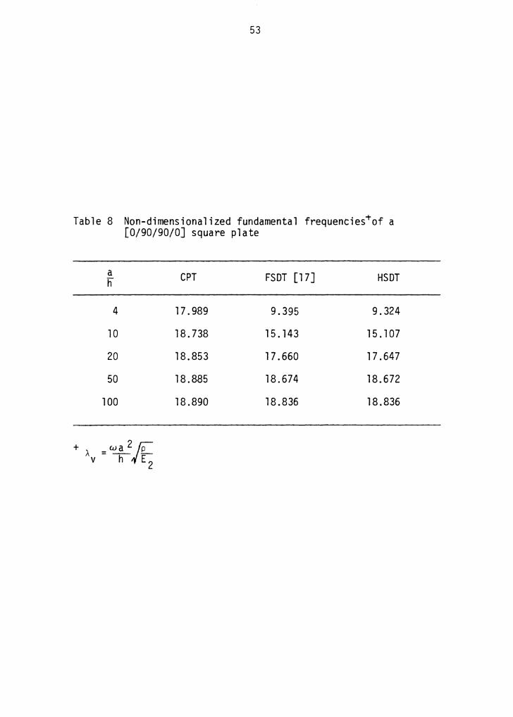
Non-dimensionalized fundamental frequencies of a [0/90/90/0] square plate ........... .

Non-dimensionalized fundamental frequencies of [8/-8/ ... ] anti-symmetric angle-ply square plates

Non-dimensionalized fundamental frequencies of a square [0/90/90/0] cross-ply as a function of modulus ratios (Material II, a/h = 5) .....

Effect of reduced integration on frequencies of a [0/90/90/0] square plate (Material II, 4x4 mesh) .

Nondimensionalized frequencies of a [45/-45Js square plate with different boundary conditions (Material II, 4E-R) ........... .

viii

31

34

37

38

44

48

49

53

55

57

61

63

Table

13

14

15

16

17

18

19

Nondimensionalized frequencies of a [0/±45/90Js square plate with different boundary conditions (Material II, 4E-R) ........... .

Nondimensionalized buckling of a [0/90/90/0] ·cross-ply square plate . . . . . . . . . ...... .

Effect of material anisotropy on the buckling loads of a [0/90/90/0] square plate (a/h = 10) ... .

Nondimensionalized buckling loads of [e/-e/ ... ] anti-symmetric angle-ply plates ....... .

Effect of reduced integration on the buckling loads of a [0/90/90/0] square plate (Material II, 4x4 mesh) . . . . . . . . . . . . . . . . . . .

Nondimensionalized buckling loads of a [45/-45Js square plate with different boundary conditions (Material II, 4E-R) ............. .

Nondimensionalized buckling loads of a [0/±45/90Js square plate with different boundary conditions (Material II, 4E-R) .............. .

ix

64

65

66

69

72

75

76

Figure

l

2

3

4

5

6

7

8

9

10

11

12

13

14

-LIST OF FIGURES

Coordinate system of a rectangular laminated plate

Coordinate system of a lamina

Deformation of a typical cross-section of the plate

Sign convention for the stress resultants

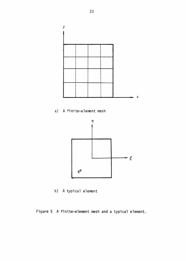
A finite-element mesh and a typical element

A four-node rectangular element and its nodal unknowns .................. .

Maximum deflections of a [0/90/90/0] square simply supported plate under sinusoidal loading (Material I).

Distribution of transverse shear stresses of a square [0/90/90/0] cross-ply plate subject to sinusoidal loading (Material I, a/h = 10) ........ .

Effect of material anisotropy on the deflections of a [0/90/90/0] square plate subjected to sinusoidal loading (Material I, a/h = 10) ........ .

Effect of material anisotropy on the deflections of [0/90/ ... ] anti-symmetric cross-ply square plates subjected to sinusoidal loading (Material I, a/h = 10) . . . . . . . . . . . . . . . . . . . .

Effect of material anisotropy on the deflections of [45/-45/ ... ] anti-symmetric angle-ply square plate subjected to sinusoidal loading (Material II, a/h = l O) . . . . . . . . . . . . . . . . . . .

Boundary conditions for a quarter of the simply supported (S-1) plate ............ .

A comparison of maximum deflections of square [45/-45/ ... ] anti-symmetric angle-ply plates sub-jected to sinusoidal loading (Material II)

Boundary conditions for a simply supported (S-2) quarter plate . . . . . ....... .

x

6

7

9

17

23

26

29

33

36

40

41

43

47

50

Figure

15

16

17

18

19

20

21

22

23

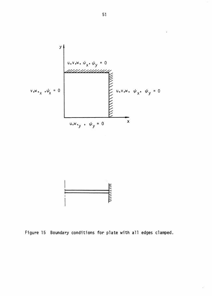
Boundary conditions for plate with all edges clamped ................ .

Nondimensionalized fundamental frequencies of [0/90/ ... ] anti-syrrmetric cross-ply square plates

Effect of material anisotropy on the frequencies of [0/90/ ... ] anti-symmetric cross-ply square plates (a/h = 5) ................ .

Effect of material anisotropy on the frequencies of [45/-45/ ... ] anti-symmetric angle-ply square plates (a/h = 10) ................... .

A comparison of frequencies of [45/-45/ ... ] anti-symmetric angle-ply square plates (Material II, 4E- R) • • • • • • • • . • • • . • . • . . . . .

Nondimensionalized buckling loads of [0/90/ ... ] anti-symmetric cross-ply plates ....... .

Effect of material anisotropy on the buckling loads of [0/90/ ... ] anti-symmetric cross-ply square plates (a/h = 10) ................ .

Effect of material anisotropy on the buckling loads of [45/-45/ ... ] anti-symmetric angle-ply square plates (a/h = 10) ................ .

A comparison of buckling loads of [45/-45/ ... ] anti-symmetric angle-ply square plates (Material II, 4E-R) •..•.••.••...•••...••••

xi

51

54

58

59

60

68

70

71

73

1.1 Motivation

CHAPTER I

INTRODUCTION

In recent years, advanced composite materials are being used in-

creasingly in many engineering and civilian applications, ranging from

the fuselage of an airplane to the frame of a tennis racket. The high

stiffness-to-weight ratio, coupled with the flexibility in the selection

of lamination scheme that can be tailored to match the design require-

ments, make the laminated plates attractive structural components for

automotive and aerospace vehicles. The increased use of laminated plates

in structures has created considerable interest in the analysis of such

structures.

Due to the high ratio of in-plane modulus to transverse shear

modulus, the shear deformation effects are more pronounced in the com-

posite laminates subjected to transverse loads than in the isotropic

plates under similar loading. The classical plate theory (CPT), in

which the Kirchhoff-love assumption that normals to the mid-surface be-

fore deformation remain straight and normal to the mid-surface after

deformation is used, is not adequate for the flexural analysis of

moderately thick laminates.

Many refined theories have been introduced to account for the

transverse shear strains. Yang, Norris and Stavskey [l] proposed a

shear deformation theory that is essentially an extension of the Mindlin

plate theory for isotropic plates to laminated anisotropic plates (also,

2

see Whitney and Pagano [2]). In this theory the transverse shear strains

are constant through the thickness, and hence shear correction coef-

ficients are used to estimate the transverse shear stiffnesses. Since it

it known that the true distribution of transverse shear stresses is

approximately parabolic through the thickness of the plate, other higher-

order theories have been proposed (see [3]). These higher-order theories

are cumbersome because with each term in the thickness coordinate an

additional dependent variable is introduced.

Recently, Reddy [4] suggested a higher-order theory in which the

inplane displacements are assumed to vary cubically through the thick-

ness, and the transverse displacement is assumed to be constant through

the thickness. The additional dependent unknowns introduced in the

higher-order theory are eliminated by imposing the boundary conditions

of vanishing transverse shear stresses on the bounding planes of the

plate. The present study is based on this theory. Exact and finite

element solutions are developed for laminated plates. A more complete

background literature for the present study is given in the next section.

1 .2 Background

Numerous shear deformation theories have been proposed to date in

the literature. Reissner [5] is the first one to investigate the effect

of transverse shear deformation on the bending of isotropic plates.

Reissner 1 s theory is based on the stress field that is derived from the

stress-equilibrium equations. Hencky [6] presented a shear deformation

theory that is based on a kinematic field. Mindlin [7] exploited

Hencky's displacement field to study the influence of shear deformation

3

on the flexural vibrations of isotropic plates.

The first shear deformation theory for laminated plates was in-

troduced by Stavsky [8]. Yang, Norris and Stavsky [l] are credited with

generalizing the Reissner-Mindlin theory to arbitrary laminated plates.

With the appropriate shear correction coefficients, the YNS theory has

been shown to be adequate in predicting the deflections, natural fre-

quencies and buckling loads for laminated anisotropic plates. Apparent-

ly, Whitney and Pagano [2] were the first ones to present closed-form

solutions for static bending and free vibration of anti-symmetric cross-

ply and angle-ply plates using the YNS theory.

Other refined theories, that account for the transverse shear de-

formation, are also available in the literature. These theories are

based on displacement fields that are expanded in powers of the thick-

ness coordinate. Whitney and Sun [9], and Lo, Christensen and Wu [3] in-

troduced such higher-order theories. However, these theories do not

satisfy the stress-free boundary conditions and require the use of shear

correction factors. Levinson [10] and Murthy [11] used cubic displace-

ment fields to develop shear deformation theories that give parabolic

distribution of the transverse shear stresses. These theories do not

require shear correction coefficients, and satisfy the stress-free con-

ditions on the bounding surfaces of the plate. Unfrotunately, these

authors did not use a variational approach to derive the associated equa-

tions of equilibrium, but used the equilibrium equations of the classical

plate theory; hence, the full contributions of the higher-order terms are

not included. Recently, Reddy [4] corrected this inconsistency and

presented a nonlinear theory.for elastic plates. The present study is

4

undertaken to fully investigate the accuracy of the new theory in pre-

dicting deflections, stresses, natural vibrations, and buckling loads.

The first finite-element analysis of laminated composite plates

that accounts for the transverse shear stresses is due to Pryor and

Barker [12]. Mau, Tong, and Pian [13], and Mau and Witmer [14] analyzed

the behavior of thick composite laminates by employing hybrid-stress

elements. Using a "mixed" formulation, Noor and Mathers [15,16] investi-

gated the effects of material anisotropy and transverse shear deformation

on the response of laminate plates. Based on the YNS theory, Reddy and

Chao [17], and Reddy [13,19] formulated a simple finite element model

to calculate the deflections and natural frequencies for cross-ply and

angle-ply laminates.

1.3 Thesis Objective

The objective of this thesis is to fully investigate the accuracy

of the higher-order shear deformation theory (HSDT) in predicting

the deflections, natural frequencies and buckling loads for laminated

composite plates. More specifically, three major objectives are identi-

fied:

l. Obtain closed-form solutions for certain laminated plates with

simply suppor.ted boundary conditions.

2. Develop a finite element model based on the displacement formu-

lation (i.e., total potential energy functional) to solve a more general

type of laminated plates with arbitrary boundary conditions.

3. Compare the present solutions with the previously reported

results to assess the accuracy of the theory and finite element developed.

-CHAPTER II

THEORY FORMULATION

2.1 Displacement Field

In developing the theory, the following assumptions are made:

1. The transverse deflection, w, is small relative to the plate

thickness so that products of the derivatives of all deflections can be

neglected in the strain-displacement equations.

2. The rotations of normals to the mid-plane, wx and wy' are

assumed to be small so that their products (i.e.,~~' wxwy' and w;) can

be neglected.

3. The transverse normal stress, crz, is negligible compared to

the in-plane and transverse shear stresses.

4. For buckling analysis, the prebuckling deformation is assumed

to be negligible.

Consider a rectangular laminated plate with dimensions a and b and

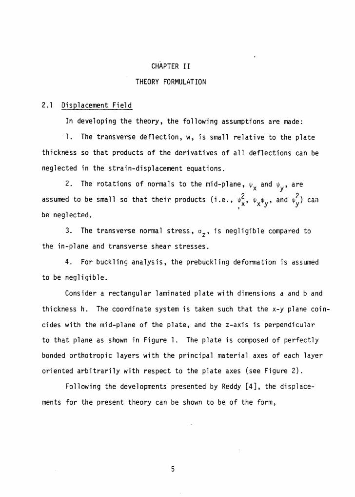
thickness h. The coordinate system is taken such that the x-y plane coin-

cides with the mid-plane of the plate, and the z-axis is perpendicular

to that plane as shown in Figure 1. The plate is composed of perfectly

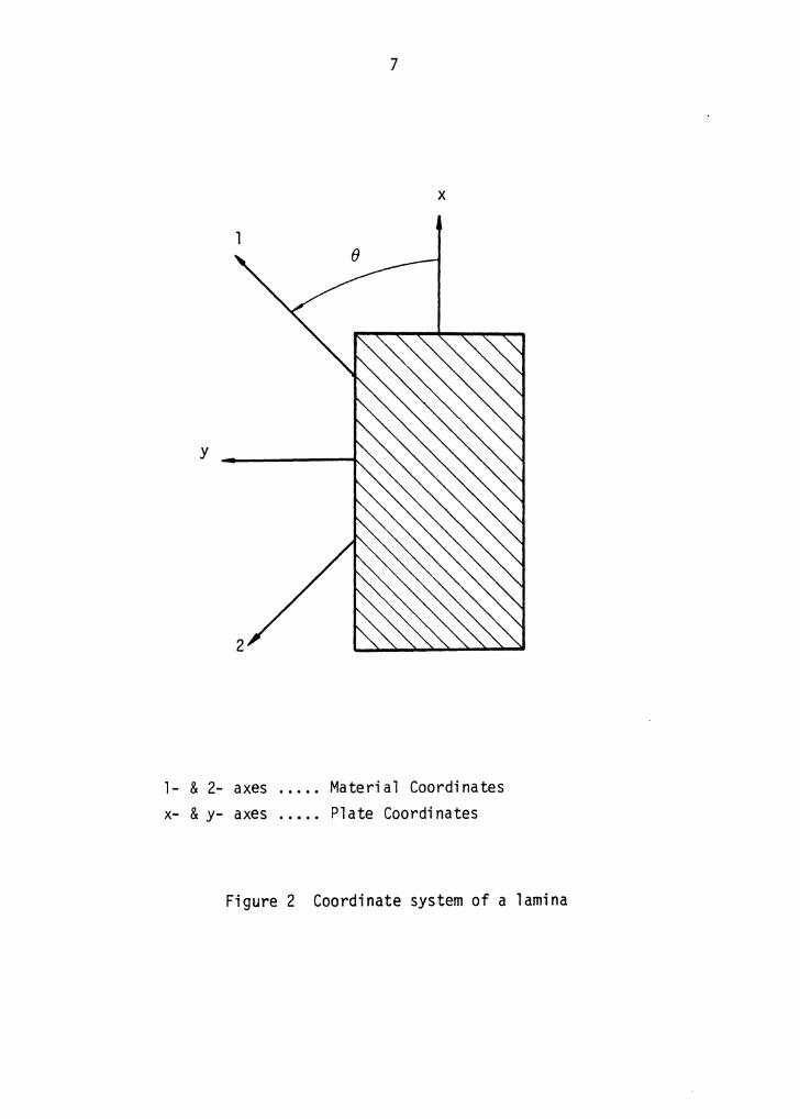
bonded orthotropic layers with the principal material axes of each layer

oriented arbitrarily with respect to the plate axes (see Figure 2).

Following the developments presented by Reddy [4], the displace-

ments for the present theory can be shown to be of the form,

5

6

R

y .[

Figure 1 Coordinate system of a rectangular laminated plate.

l

y

1- & 2- axes x- & y- axes

.7

x

Material Coordinates Plate Coordinates

Figure 2 Coordinate system of a lamina

8

4 (z) 2 u1(x,y,z,t) = u(x,y,t) + z[$x(x,y,t) - 3 hJ ($x(x,y,t)

+ ~~ ( x ,y 't) ) ]

4 (z) 2 u2(x,y,z,t) = v(x,y,t) + z[$Y(x,y,t) - 3 h ($Y(x,y,t)

+ ~~ ( x ,y ' t ) ) ]

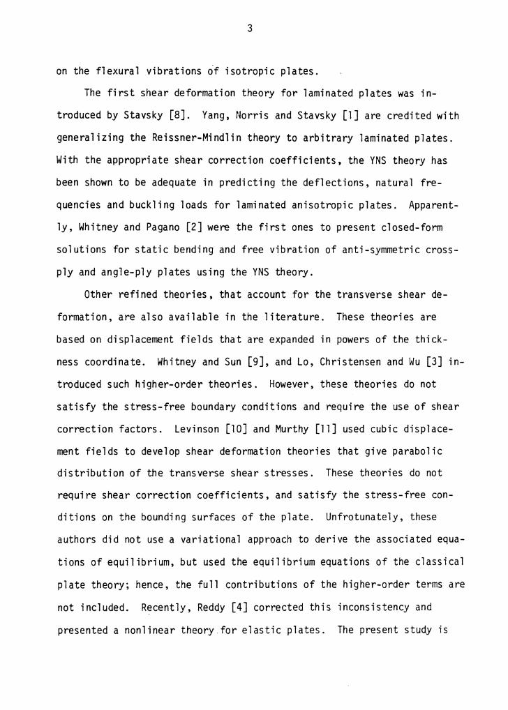
u3(x,y,z,t) = w(x,y,t) (2.1.l)

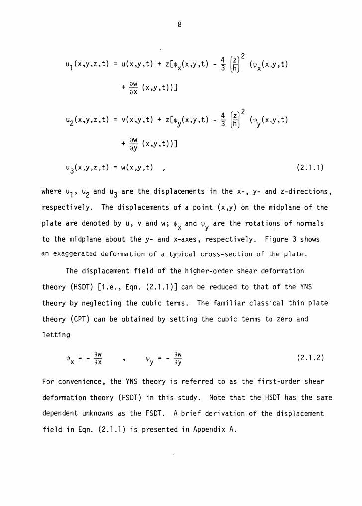
where u1 , u2 and u3 are the displacements in the x-, y- and z-directions,

respectively. The displacements of a point (x,y) on the midplane of the

plate are denoted by u, v and w; $x and $ are the rotations of normals y -to the midplane about they- and x-axes, respectively. Figure 3 shows

an exaggerated deformation of a typical cross-section of the plate.

The displacement field of the higher-order shear deformation

theory (HSDT) [i.e., Eqn. (2.1.1)] can be reduced to that of the YNS

theory by neglecting the cubic terms. The familiar classical thin plate

theory (CPT) can be obtained by setting the cubic terms to zero and

letting

ljJ = x aw ax

aw ljJ = Y - ay (2.1.2)

For convenience, the YNS theory is referred to as the first-order shear

deformation theory (FSDT) in this study. Note that the HSDT has the same

dependent unknowns as the FSDT. A brief derivation of the displacement

field in Eqn. (2.1 .1) is presented in Appendix A.

9

u

w z

----------

Figure 3 Deformation of a typical cross-section of the plate.

10

2.2 Strain-Displacement Relations

In the linear theory of elasticity, the strains are related to the

displacement gradients by

(2.2.l)

where i,j = 1,2,3,

and the comma denotes differentiation (i.e., u. J. = au./ax.). l ' l J

Substituting the displacements from Eqn. (2.1 .1) into Eq. (2.2.1),

the following strain-displacement equations are obtained:

~ = ~ ~o + z (Ko + z2 2) c2 c22 = c2 2 K2

(2.2.2)

where

o _ au e1 - ax ,

eo _ ,,, + aw 5 - "'x ax

2.3 Constitutive Equations

11

(2.2.3)

Assuming that each layer possesses a plane of material symmetry

parallel to the x-y plane, the constitutive equations for the k-th layer

can be written as

- (k) - (k) - (k) al Qll Ql2 0 el

-a2 = Ql2 Q22 0 -€2 -- -

a6 0 0 Q66 €6

{::r) . [Q~4 _or) {~4r (2.3.1) Q55 €5

where cri and ei (i = 1,2,4,5,6) are the stress and strain components

referred to lamina coordinates and Qij's are the plane-stress reduced

elastic constants in the material axes of the k-th lamina,

E2 022 = -, ---v-1 2_v_2_1

(2.3.2)

12

Transformed to the plate (i.e., laminate) coordinates, the lamina

stress-strain relations in Eqn. (2.3.l) become:

cr l (k)

= SyJTVTI.

[Q Q l(k) {e }(k) 44 45 4 Sym. 055 e5

(2.3.3)

where Qij's are the transformed material stiffness coefficients Qij of

the k-th layer.

2.4 Equations of Motion

The equations of motion can be obtained using the Hamilton's

principle. In analytical form, the principle can be stated as follows:

t J J (oU + oW - oT) dV dt = o 0 vol.

where U is the total strain energy due to deformation,

W is the work done by external loads, and

T is the kinetic energy of the plate,

and o denotes the variational symbol.

(2.4.l)

Substituting appropriate energy expressions into the above equa-

tion (see Reddy and Rasmussen [20]), Eqn. (2.4.l) becomes:

13

- J q ow dx dy + J { (N aw + N awJ ow, + (N aw R R xo ax xyo ay x xyo ax

(2.4.2)

where p denotes the density, q the applied transverse loading, and

Nxo' Nyo and Nxyo denote the in-plane applied loads (in the case of

buckling analysis).

Substituting the strain-displacement relations in Eqn. (2.2.2) into

the above equation, and integrating through the thickness of the laminate,

Eqn. (2.4.2) can be expressed as:

0 = J: {JR Nl ou,x + Ml O>x,x + Pl [- 3~2 (O>x,x + ow,xx)]

+ N2 ov,Y + M2 o$y,y + P2 [- 3~2 (o$y,y + ow,YY)}

+ N6(ou,Y + ov,x) + M6(owx,y + owy,x)

+ P6 [- 3~2 (owx,y + o$y,x + 2ow,xy)] + Q2(owy + ow,Y)

+ R2 [- ~· (o$Y + ow,Y)J + Q1(o$x + ow,x)

+ R1 [- h~ (o$x + ow,x)] - q ow+ ·(Nxo w,x + Nxyo w,Y) ow,x

+ (Nxyo w,x + Nyo w,Y) ow,Y}dxdydt

14

t - J J {[r, u + (I2 - 42 I4) ~x - ~ I4 w, ] OU

0 R 3h 3h x

( 8 16 ) .. 4 ( 4 ) .. J + I3 - -2 I5 + 4 I7 tiix - -2 I5 - -2 I7 w,x oljix 3h 9h 3h 3h

[( 4 ) .. ( 8 16 ) .. + 12 - -2 14 v + 13 - -2 I5 + 4 17 ljiy

3h 3h 9h

4 ( 4 , .. J }d d - - 2 I 5 - - 2 I 7 w 'y oljiy x dy t 3h 3h

where the stress resultants N1., M., P., Q. and R. are defined by 1 1 1 1

rh

(N1 ,N2 ,N6) = J =!!. (a1 ,a2 ,a6) dz 2

h (M1,M2,M6) = J2h (a1 ,a2,cr6) z dz

2

h

(P1 ,P2,P6) = I=!!. (a1 ,cr2,a6) z3 dz 2

(2.4.3)

15

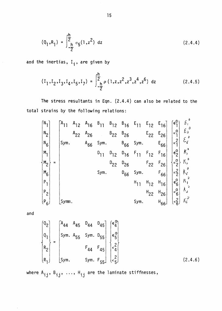
h Jz 2 (2.4.4) (Q1,R1)= hcr5{1,z)dz -2

and the inertias, Ii' are given by

h Jz 2 3 4 s dz (2.4.5) (!1 ,I2,r3,r4,r5,r7) = hp (l,z,z ,z ,z ,z ) -2

The stress resultants in Eqn. (2.4.4) can also be related to the

total strains by the following relations:

Nl All A12 Al6 811 812 816 Ell E12 El6 eo &,o l

£::/ N2 A22 A26 822 826 E22 E26 KO 1

[ 0

N6 Sym. A66 Sym. 866 Sym. E66 2 Kl (

Ml 011 o,2 o,6 Fll Fl2 Fl6 eo 2 K,()

M2 022 026 F22 F26 0 K;,o = K2

M6 Sym. 066 Sym. F66 K2 2 ~: €0

;)

pl Hll Hl2 Hl6 /\I 6 :i

p2 H22 H26 0 Aa K6

K2 d p6 Symm. Sym. H66 f(G 6

and

021 A44 A45 044 045 €4

Ql Sym. A55 Sym. 055 eo 5

R2r F44 F45 2 K4

Rl Sym. Sym. F55 2 (2.4.6) K5

where A .. , lJ Bij' ... , H .. lJ are the laminate stiffnesses,

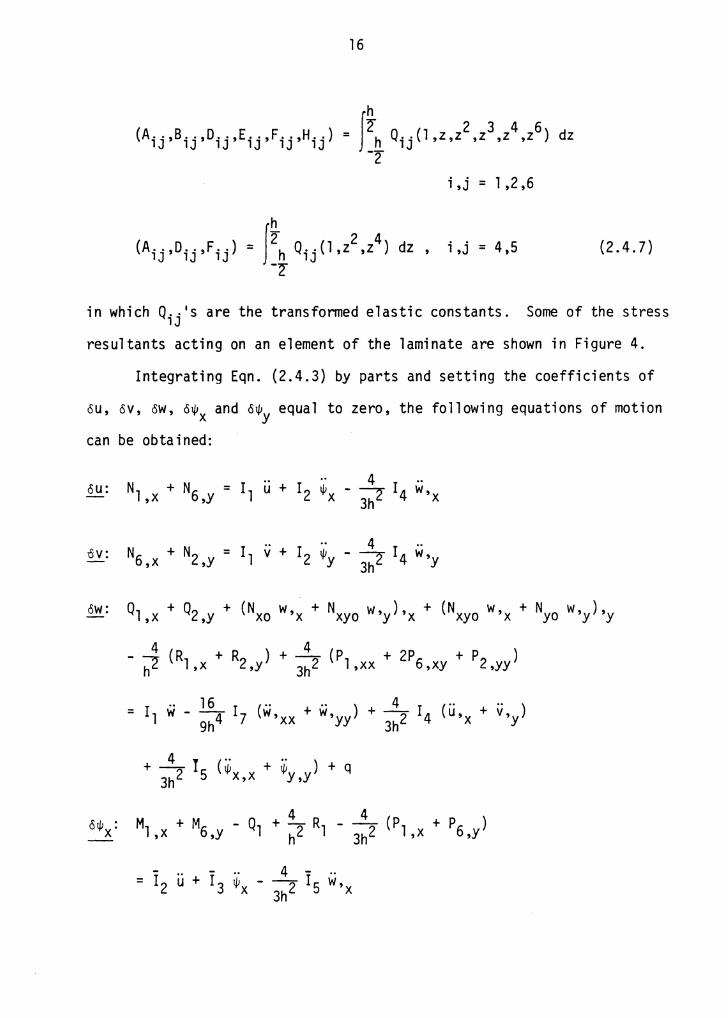
16

h

f 2 2 3 4 6 (A .. ,B .. ,o .. ,E..,F .. ,H .. ) = _!!_Q1.J.(l,z,z ,z ,z ,z) dz lJ lJ lJ lJ lJ lJ 2

i ,j = 1 ,2 ,6

h

f2 2 4 (A .. ,o .. ,F .. ) = h Q .. (l,z ,z) dz , lJ lJ lJ lJ -2 i ,j = 4 ,5 (2.4.7)

in which Qij•s are the transfonned elastic constants. Some of the stress

resultants acting on an element of the laminate are shown in Figure 4.

Integrating Eqn. (2.4.3) by parts and setting the coefficients of

au, av, ow, ol/Jx and ol/JY equal to zero, the following equations of motion

can be obtained:

N + N = I1 u + 12 l/JX 4 .. au: - -:2" 14 w,x l,x 6,y 3h

N + N = I1 ii + .. 4 .. -CV: 6,x 2,y 12 l/Jy - 3h2 14 w,y

ow: Q1 +Q2 +(N w, +N w,), +(N w, +N w,), ,x ,y xo x xyo y x xyo x yo y y

- 4 (R + R ) + _!__ (P + 2P + P ) ~ 1 ,x 2,y 3h2 1 ,xx 6,xy 2,yy

4 4 olj!x: Ml + M6 - Ql + -2 Rl - -2 (Pl + p6 y) ,x ,y h 3h ,x '

17

a) Forces

b) Moments

Figure 4 Sign convention for the stress resultants.

18

o~ : M + M - Q + 4 R - ~ (P + P ) ~ 6,x 2,y 2 t;2 2 3h2 6,x 2,y

(2.4.8)

where

I = r3 - ~ I + 16 I 3 3h2 5 9h4 7

(2.4.9)

The integrations also yield the following boundary conditions:

Natural:

on r, where r is the boundary of the midplane of the plate, and

u = u n + v n n x y

A 4 M. = M. - - P

1 l 3h2 i

u = - u n + v nx ns y

2 - n ) y

(i = 1,2,6)

(i = 1,2,6)

(2.4.10)

19

-Nn = (N1 w,x + N6 w,Y) nx + (N6 w,x + N2 w,Y) ny

a a a -=n -+n an x ax y ay a a a - = n - - n as x ay y ax (2.4.11)

where nx and ny denote the components of the normal vector along the

boundary of the midplane.

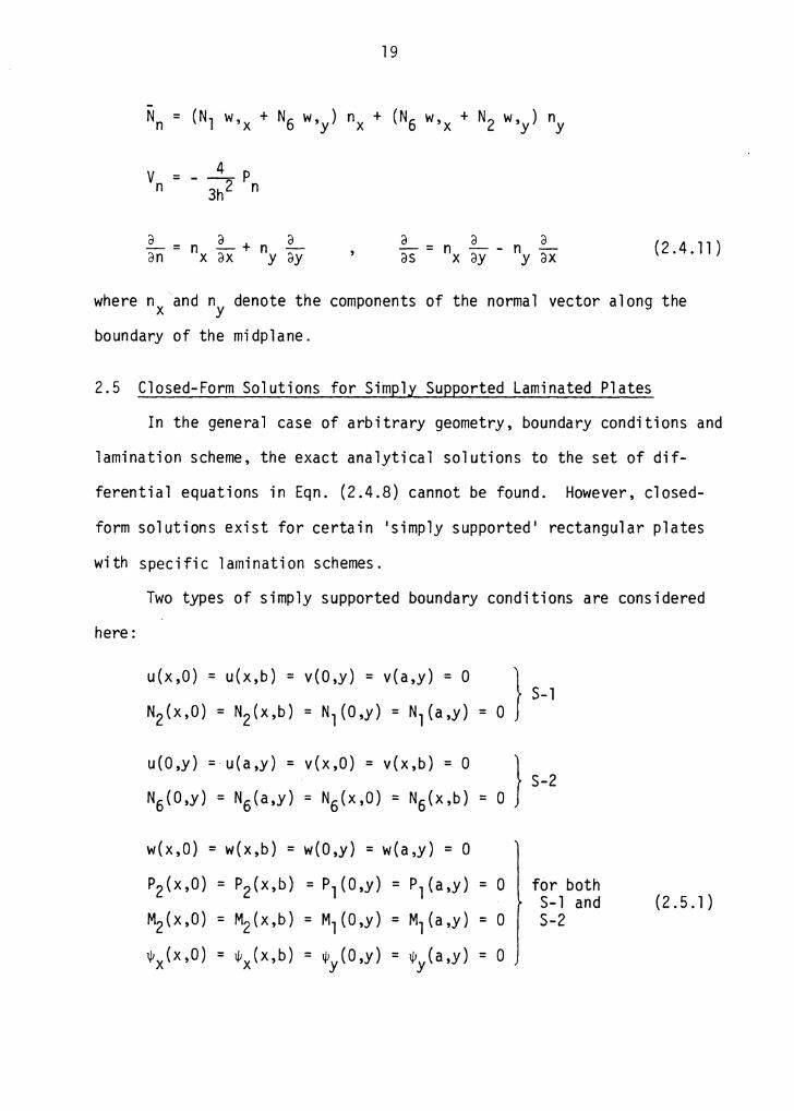
2.5 Closed-Form Solutions for Simply Supported Laminated Plates

In the general case of arbitrary geometry, boundary conditions and

lamination scheme, the exact analytical solutions to the set of dif-

ferential equations in Eqn. (2.4.8) cannot be found. However, closed-

form solutions exist for certain 'simply supported' rectangular plates

with specific lamination schemes.

Two types of simply supported boundary conditions are considered

here:

u(x,O) = u(x,b) = v(O,y) = v(a,y) = 0 } 0 S-1

N2(x,0) = N2(x,b) = N1(0,y) = N1(a,y) =

u(O,y) = u(a,y) = v(x,0) = v(x,b) = 0 } 0 S-2

N6(0,y) = N6(a,y) = N6(x,0) = N6(x,b) =

w(x,0) = w(x,b) = w(O,y) = w(a,y) = 0

P2(x,O) = P 2 ( x, b) = P 1 ( 0 ,y) = P 1 (a ,y) = 0 for both S-1 and

M2(x,O) = M2(x,b) = M1 ( 0 ,y) = M1 (a ,y) = 0 S-2

iJix(x,O) = ijJX(X,b) = iJiy(O,y) = iJiy(a,y) = 0

(2.5.l)

20

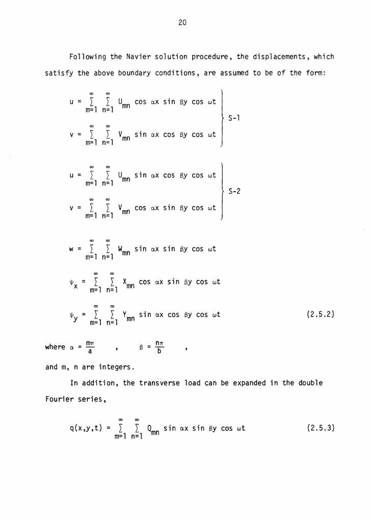
Following the Navier solution procedure, the displacements, which

satisfy the above

00

u = l m=l

00

v = I m=l

00

u = I m=l

00

v = l m=l

00

w = l m=l

00

I/Ix = l m=l

00

l/ly = I m=l

ffi1T where o. = -a

00

l n=l

00

I n=l

00

l n=l

00

l n=l

00

I n=l

00

I n=l

00

I n=l

boundary conditions, are assumed

Umn COS o.X sin BY cos wt

S-1

vmn sin ax cos BY cos wt

umn sin ax cos BY cos wt

S-2

Vmn COS o.X sin By cos wt

wmn sin o.X sin BY cos wt

xmn cos ax sin BY cos wt

Ymn sin o.x cos BY cos wt

n1T B = b

and m, n are integers.

to be of the form:

(2.5.2)

In addition, the transverse load can be expanded in the double

Fourier series,

00 00

q{x,y,t) = I I Qmn sin ax sin By cos wt m=l n=l

(2.5.3)

21

With the above displacements, closed-form solutions can be obtained

for plates with lamination schemes such that

S-l: Al6 = A26 = 816 = 826 = Dl6 = D26 = O

El6 = E26 = Fl6 = F26 = Hl6 = H26 = O

A45 = D45 = F45 = O

S-2: Al6 = A26 = 811 = 812 = 016 = 026 = 0

Ell = El2 = Fl6 = F26 = Hl6 = H26 = O

A45 = D45 = F45 = O (2.5.4)

These two sets of conditions are satisfied by general cross-ply and anti-

syrrmetric angle-ply laminates, respectively.

Substitutions of Equations (2.5.2) and (2.5.3) into Eqn. (2.4.8),

give

[K]{6} = {F} + Av [M]{6} + Ab [G]{6} (2.5.5)

for any fixed values of m and n. Here

and Av denotes the square of the natural frequency, and Ab is the buckling

load parameter. The elements of stiffness matrix [K], mass matrix [M]

and matrix [G] are given in Appendix 8.

For static bending, Eqn. (2.5.5) is simplified to a set of simul-

taneous equations. Once the amplitudes are solved for, the generalized

displacements can be calculated for any point on the plate. The stresses

22

can be obtained using constitutive equations.

For free vibration and stability analysis, the equation in

(2.5.5) is reduced to a standard eigenvalue problem. Note that the

buckling loads for plates subjected to pure shear loading cannot be

determined exactly.

2.6 Finite-Element Formulation

Based on the HSDT, a finite element model is formulated to analyze

general laminated plates with arbitrary edge conditions.

Consider the midplane, R, that is subdivided into a mesh of finite

elements as shown in Figure 5. Over a typical element, a variational

form of the equations of motion in Eqn. (2.4.8) is given by

4 [I 1

.. .. 4 .. + [M2 - -2 P2] t'lljly ,y + u + 12 l/! - -2 I4 w, J 8U

3h, x 3h x

ii + i2 ~y 4 .. J n2

.. .. + [Il - -2 I4 w, 8V + u + I3 wx 3h y

23

y

x

a) A finite-element mesh

b) A typical element

Figure 5 A finite-element mesh and a typical element.

24

- --; 15 w, J 61/l + n2 v + 1 ~: - -4- r w, J Ot;,' 3h x x 3 y 3h2 5 y y

4 .. 4 - .. 16 .. J + r1 w ow + [- - 2 r4 u - - 2 r5 tJi + - 4 I7 w, 3h 3h x 9h x

+ [Nxo w,x + Nxyo w,Y] ow,x + [Nxyo w,x + Nyo w,Y] ow,Y} dxdy

+ I (Nn OU + N OU ) ds + I (Qn ow + vn ow,n) ds C n ns ns C N q

+ J (Mn otJin + Mns otJins) ds (2.6.1) CM

The displacements can be interpolated over an element by the fol-

lowing expressions (see Reddy [21]):

n u(x,y,t) = I u. <t>i(x,y) cos wt

i =l l

n v(x,y,t) = I v. <t>i(x,y) cos wt

i = 1 l

m w(x,y,t) = I w Q, 1Ji Q, ( x ,y ) COS wt

£=1

s tJix(x,y,t) = I x. ~i(x,y) cos wt

i =l l

s lJ!y(x,y, t) = I Yi ~i ( X ,y) COS wt

i =l (2.6.2)

where Ui' Vi, W£, Xi, Yi are the displacements at nodal points,

25

-and ;i, ~ 1 , ~i are the interpolation functions.

For simplicity, the same shape functions will be employed for the

in-plane displacements and the two rotations. From Eqn. (2.4.10), the

variational formulation requires that the transverse deflection and its

derivatives ·be continuous across the interelement boundary; hence, the

interpolation functions for w must be at least of cubic order.

Combining Equations (2.6.1) and (2.6.2) and collecting like terms,

the element equations can be obtained:

(2.6.3)

where {~} denotes a vector of generalized nodal displacements, and {F}

is the force vector that contains the applied transverse load as well as

the contributions from the b9undary of a domain. The coefficients of

matrices in the above equation are listed in Appendix C.

In the present study, four-node rectangular elements are used. The

in-plane displacements and the two rotations, wx and wy' are interpolated

over an element by linear isoparametric functions. On the other hand,

a set of non-conforming cubic shape functions (see Zienkiewicz [22]) are

employed for the transverse deflection. In Figure 6, the seven degrees

of freedom (three displacements, two shapes and two rotations) at each

node are shown. All of the shape functions are given in Appendix D for

convenience.

The governing equations in (2.6.3) are computed for each dis-

cretized element. After assembling the elements and imposing the speci-

fied boundary conditions, the solutions then can be obtained. For

additional details consult the finite element book by Reddy [21].

(-1,1) 4

(-1,-1)

ul vl wl

W5= (w,x)l w9= (w,y)l

x, yl

26

'

( 1 '1) 3

2 ( 1 ,-1)

Figure 6 A four-node rectangular element and its nodal unknowns.

CHAPTER III

NUMERICAL RESULTS AND DISCUSSION

In this chapter, closed-form solutions of simply supported lami-

nated plates predicted by the higher-order shear deformation theory

(HSDT) are presented and compared with the results of other theories.

The effects of transverse shear deformation, material anisotropy and

coupling between stretching and bending on the deflections, frequencies,

and buckling loads of plates are also investigated. The finite element

model developed herein is validated by comparing the results with the

exact solutions. Once the accuracy of the finite element model has been

verified, analyses of general laminates with arbitrary edge conditions

are conducted.

In most of the problems considered, two sets of material proper~

ties are used:

Material I:

= 0.25

Mate ri a 1 I I :

It is assumed further that G12 = G13 , v 12 = v 13 and o = 1. And for the

analysis based on the FSDT, shear correction coefficients of k~ = k~ = ~

are used.

27

28

3.1 Bending Analysis

Consider a four-layer [0/90/90/0] square cross-ply laminated plate

(Material I) subjected to sinusoidal loading. The plate is simply sup-

ported (S-1) on all four edges with the in-plane displacements free

to move in the normal direction and constrained in the tangential direc-

tion. The deflections and stresses are non-dimensionalized as

follows:

w(~ a 0) E h3 - 2 '2 ' 2 x 102 w =

qo a4

- h2 ol = ol

qo a2

(3.l.l) h2

= 06 06 qo a2

- h 05 = 05 qo a

In Figure 7, the maximum deflections for various side-to-thickness ratios

are compared. The deflections predicted by the HSDT are in excellent

agreement with the 3-D elasticity solutions of Pagano and Hatfield [23].

In the range of medium to thick plates (* .::_ 20), the HSDT

2.0

\ / 3-0ES

1.8

1.6

\\ ·~ .I /- llSDT 1.4

1.2 I I\\

w ... FSOT

1.0

0.8

0.6

~----------------__;.::_:_-==:=;~--··-~--~ 0.4 J___-------;;;:;;--~~~===-----0.0 10.0 20.0 30.0 40.0 50.0

a ii

Figure 7 Maximum deflections of a [0/90/90/0] square simply supported plate under sinusoidal loading (Material I).

N l.O

30

yields more accurate results than the FSDT. The effect of shear deforma-

tion on the deflections can be seen clearly from the results. As Whitney

[24] has shown previously, the shear deformation causes the reduction in

stiffness of composite plates and is more pronounced with the decreasing

side-to-thickness ratios. However, the CPT is adequate in predicting

the deflections of thin laminated plates (a/h .:::_ 50) in comparison with

the other theories.

Table 1 contains stresses o1, o2 , and 0 6 computed by the HSDT,

which are greatly improved over the results obtained using the CPT and

the FSDT. The shear stresses obtained using constitutive equations are

on the low side of the 3-D elasticity solutions. This error might be

due to the fact that the stress continuity across each layer interface

is not imposed in the present formulation. As in the case of the CPT,

the transverse shear stresses can also be determined by integrating the

stress equilibrium equations through each lamina:

(3.1.2)

where the body forces are neglected.

The above approach not only gives single-valued shear stresses at the

interfaces but yields excellent results in comparison with the 3-D solu-

tions. Despite its apparent advantage, the use of stress equilibrium

conditions is mathematically inconsistent with two-dimensional plate

Table l Non-dimensionalized stresses of a square [0/90/90/0] simply supported laminate under sinusoidal loading (Material I)

- - - ; 4 (~,o,o) o5 (O,~,O) a Source o l 02 06

h (a a h) (a a h) h 2'2'2 2'2'4 (0,0,2) Const. Equil . Const. Equi l .

3-DES [23] 0. 720 0.663 0.0467 -- 0.292 -- 0.219 4 HSDT 0.6651 0.6322 0.0440 0.2389 0.2985 0.2064 0.2306

FSDT [17] 0.4059 0.5764 0.0308 0. 1962 0.2799 0. 1398 0.2686

3-DES 0.559 0.401 0.0275 -- 0. 196 -- 0. 301 10 HSDT 0.5456 0.3888 0.0268 0. 1531 0. 1924 0.2640 0.3069

FSDT 0.4989 0.3614 0.0241 0. 1292 0 .1807 0. 1666 0. 3181 w

3-DES 0.543 0.308 0.0230 -- 0 .156 -- 0.328 20 HSDT 0.5393 0.3043 0.0228 0. 1234 0. 1541 0.2825 0.3299

FSDT 0.5273 0.2957 0.0221 0.1087 0. 1503 0. 1748 0.3332

3-DES 0.539 0.276 0.0216 -- 0. 141 -- 0.337 50 HSDT 0.5387 0.2752 0.0215 0. 1132 0. 1409 0.2888 0. 3377

FSDT 0.5368 0.2737 0.0214 0.1019 0. 1402 0. 1775 0.3383

3-DES 0.539 0.271 0.0214 -- 0 .139 -- 0.339 100 HSDT 0.5387 0.2708 0.0213 0.1117 0. 1389 0.2897 0.3389

FSDT 0.5382 0.2705 0.0213 0 .1008 0. 1387 0. 1779 0.3390

CPT 0.5387 0.2694 0.0213 0.0 0 .1382 0.0 0.3393

32

theories. In addition, the integrations in Eqn. (3. 1.2) could become a

cumbersome task for laminated plates with many layers. Typical stress

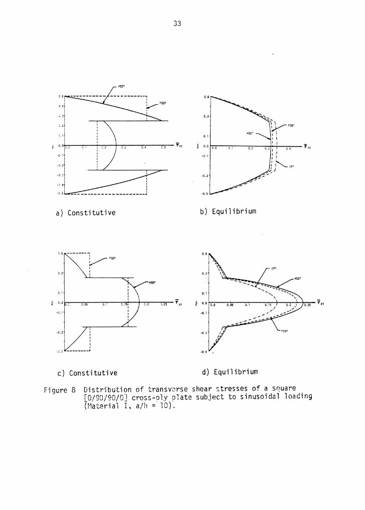
distributions of cr5 = Txz and cr4 = Tyz through the thickness (a/h = 10)

are shown in Figure 8. The parabolic stress variation can be modeled,

and the stress-free boundary conditions on top and bottom surfaces of

the plate are obviously satisfied by the HSOT. Note that the stress

discontinuity at the laminae interfaces is due to the mismatch of the

transformed material properties.

By considering the cylindrical bending of an orthotropic laminate,

Whitney [25] determined analytically the shear coefficients. For the

[0/90/90/0] cross-ply (Material I), the suggested shear correction fac-

tors are given by

2 kl = 0.5952 2 k2 = 0.7205 (3.1.3)

Table 2 contains a comparison of results obtained using the FSOT with two

sets of shear correction factors with those obtained using the HSOT and

the 3-0 elasticity theory for various side-to-thickness ratios. Clearly,

the deflections with the shear factors in Eqn. (3.1 .3) are in

closer agreement with the results of HSOT and 3-0 elasticity theory.

As Chow [26], and Noor and Mathers [27] have also shown, the shear co-

efficients are strongly influenced by the lamina properties and the

stacking sequence. Hence, no single value of these coefficients is

valid for all laminations and stacking sequence. In addition, the

approach taken by Whitney does not work for general laminates where the

cylindrical bending solutions cannot be obtained. As a result, the

shear correction factors of~ (~erived for the isotropic case) are used

33

,.s -----------., I

'·' ~~SOT

' I '·Ji :.z

I

~. i

o. --- ..... .o+.-..---...,.---.,,,-..z-+-""'.: . ..-J ----,,,.._..----• ..,.,- T.z .,::.:

-J.I

-u

' I I ' .. :.s

----------------------~

a) Constitutive

1.S --------: ~FSDT

I I I J.J

' ·0.J I I I I I ' .. ::.~ ________ J

c) Constitutive

t •

0.5

O.J

0.1

o.o f":,Oii.o~--,, . ..,., --~o.z::----:"'"'· J.+-<J.....;.........,,-_.-- ;: •: -0.1

-0.J

-o.s

b) Equilibrium

-o.s

d) Equilibrium

I I I!

: i"-rp• J) . ::.":.·''

o.2s ;: ,,

Figure 8 Distribution of transv2rse shear stresses of a square [0/90/90/0] cross-ply plate subject to sinusoidal loading (Material i, a/h = 10).

34

Table 2 Effect of shear correction coefficients on the maximum de-flections of a [0/90/90/0] square simply supported plate sub-jected to sinusoidal loading (Material I)

FSDT

a 3-DES [23] k2 = k2 = .§.. kt = 0.5952 h HSDT l 2 6 k~ = 0.7205

4 1.9367 l . 8937 1.7096 l . 9603

10 0.7370 0.7147 0.6627 0.7022

20 0.5128 0.5060 0.4912 0.5013

50 0.4446 0.4434 0.4410 0.4426

100 0.4347 0.4343 0.4337 0.4341

CPT 0.4313

35

in this study.

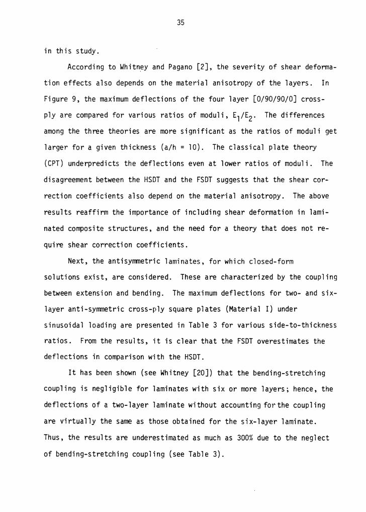
According to Whitn~y and Pagano [2], the severity of shear deforma-

tion effects also depends on the material anisotropy of the layers. In

Figure 9, the maximum deflections of the four layer [0/90/90/0] cross-

ply are compared for various ratios of moduli, E1/E2. The differences

among the three theories are more significant as the ratios of moduli get

larger for a given thickness (a/h = 10). The classical plate theory

(CPT) underpredicts the deflections even at lower ratios of moduli. The

disagreement between the HSDT and the FSDT suggests that the shear cor-

rection coefficients also depend on the material anisotropy. The above

results reaffirm the importance of including shear deformation in lami-

nated composite structures, and the need for a theory that does not re-

quire shear correction coefficients.

Next, the antisymmetric laminates, for which closed-form

solutions exist, are considered. These are characterized by the coupling

between extension and bending. The maximum deflections for two- and six-

layer anti-symmetric cross-ply square plates (Material I) under

sinusoidal loading are presented in Table 3 for various side-to-thickness

ratios. From the results, it is clear that the FSDT overestimates the

deflections in comparison with the HSDT.

It has been shown (see Whitney [20]) that the bending-stretching

coupling is negligible for laminates with six or more layers; hence, the

deflections of a two-layer laminate without accounting for the coupling

are virtually the same as those obtained for the six-layer laminate.

Thus, the results are underestimated as much as 300% due to the neglect

of bending-stretching coupling (see Table 3).

-w

2.0

l. 5

1.0

J.3

\ \

' ' \ \ \

\ ' \ ~

\ \ \ \ \ \

\\ \ \ \

\ \ \ \ \ \ \ \,

\ \ \ \

\ \\ \ \ \ \

36

\ \,,,

- HSO";"

--·- FSDT

-·· - CPT

\ ' \ ' \ ' ...................

' ' "..... ....... .....

""---- .. _ -

------ ------J.O J~~~~~~~l0.,..._~~~~~-20--~~~~~-~--~~~~~-4-0~~

Figure 9. Effect of material anisotropy on the deflections of a [0/90/90/0] square plate subjected to sinusoidal loading (Material I, a/h = 10).

37

Table 3 Maximum deflections of square [0/90/ ... ] anti-syrrmetric cross-ply simply supported plates subjects to sinusoidal loading (Material I)

a n = 2 n = 6 h FSDT HSDT FSDT HSDT

4 2. 1492 l .9985 l . 5473 l . 5411

10 l. 2373 1.2161 0.6354 0.6382

20 l. 1070 l . l 018 0.5052 0.5052

50 l . 0705 l . 0697 0.4687 0.4687

100 l . 0653 l .0651 0.4635 0.4635

CPT l . 0636 0.4618

Table 4 Maximum deflections of square [e/-e/ ... ] anti-symmetric angle-ply simply supported plates subjected to sinusoidal loading (Material II)

e = 5° e = 30° e = 45° a Source h n = 2 n = 6 n = 2 n = 6 n = 2 n = 6

4 HSDT 1.2625 1.2282 1.0838 0.8851 1 .0203 0.8375 FSDT [17] 1 . 3165 1.2647 1 . 2155 0.8994 l . 1576 0.8531

10 HSDT 0.4848 0.4485 0.5916 0.3007 0.5581 0.2745 w FSDT 0.4883 0.4491 0.6099 0.2989 0. 5773 0. 2728 00

20 HSDT 0.3579 0.3209 0.5180 0.2127 0.4897 0.1905 FSDT 0.3586 0.3208 0.5224 0.2121 0.4944 0. 1899

50 HSDT 0.3215 0.2842 0.4972 0 .1878 0.4704 0 .1668 FSDT 0.3216 0.2841 0.4979 0 .1877 0.4712 0. 1667

100 HSDT 0. 3162 0.2789 0.4942 0 .1842 0.4676 0. 1634 FSDT 0.3162 0.2789 0.4944 0 .1842 0.4678 0. 1633

CPT 0.3145 0. 2771 0.4932 0. 1831 0.4667 0. 1622

39

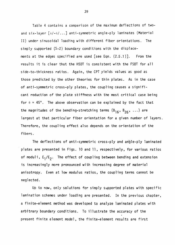
Table 4 contains a comparison of the maximum deflections of two-

and six-layer [b/-6/ ... ] anti-symmetric angle-ply laminates (Materia~

II) under sinusoidal loading with different fiber orientations. The

simply supported (S-2) boundary conditions with the displace-

ments at the edges specified are used [see Eqn. (2.5.l )]. From the

results it is clear that the HSDT is consistent with the FSDT for all

side-to-thickness ratios. Again, the CPT yields values as good as

those predicted by the other theories for thin plates. As in the case

of anti-symmetric cross-ply plates, the coupling causes a signifi-

cant reduction of the plate stiffness with the most critical case being

fore= 45°. The above observation can be explained by the fact that

the magnitudes of the bending-stretching terms (B 16 , B26 , ... )are

largest at that particular fiber orientation for a given number of layers.

Therefore, the coupling effect also depends on the orientation of the

fibers.

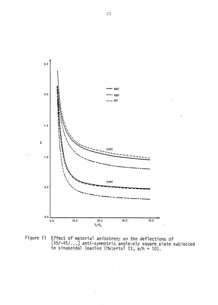
The deflections of anti-symmetric cross-ply and an~le-ply laminated

plates are presented in Figs. 10 and 11, respectively, for various ratios

of moduli, E1;E2. The effect of coupling between bending and extension

is increasingly more pronounced with increasing degree of material

anisotropy. Even at low modulus ratios, the coupling terms cannot be

neglected.

Up to now, only solutions for simply supported plates with specific

lamination schemes under loading are presented. In the previous chapter,

a finite-element method was developed to analyze laminated plates with

arbitrary boundary conditions. To illustrate the accuracy of the

present finite element model, the finite-element results are first

40

2.0

- HSDT

----- FSDT

1.5 --·- CPT

w

1.0

0.5 -...... .... -...... ..... ..

------........ ---.... -- --...... -----0.0

o.o 10.0 20.0 30.0 40.0

E1/E2

. Figure 10 Effect of material anisotropy on the deflections of [0/90/ ... ] anti-symmetric cross-ply square plates subjected to sinusoidal loading (Material I, a/h = 10).

2.5

2.0

1.5

1.0

0.5

I l ' l \\

I ~ I ~

\ '\

- HSOT

---- FSDT

-- CPT

-------------------------

\ "'-<l \ ~ (~6)

~ ~~-~.--..=-==--~------' .. ......._ __ _

------ -------

Figure 11 Effect of material anisotrory on the deflections of [45/-45/ ... ] anti-symmetric anq1e-ply square plate subjected to sinusoidal loading (Material II, a/h = 10).

42

compared with the previously known closed-form solutions. Then a finite-

element analysis is performed for some commonly used laminated plates

subjected to various loadings. The purpose of the above task is to

demonstrate the versatility of the finite-element method, and to serve

as references for future investigators.

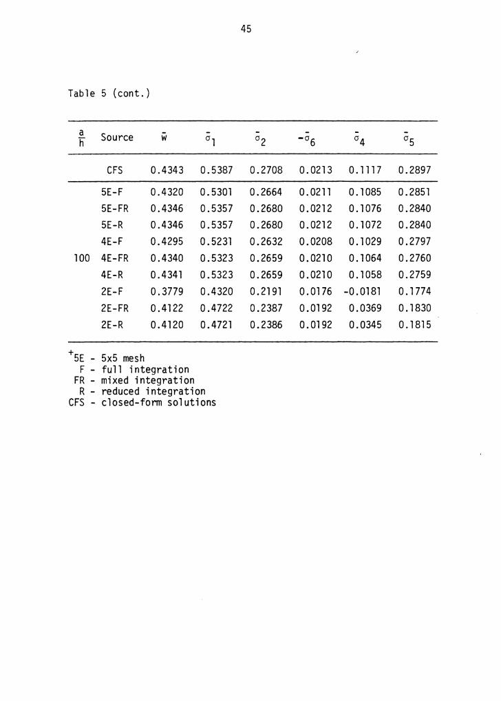
Due to the existing biaxial syrrmetry, only a quarter of the plate

is modeled. For a four-layer [0/90/90/0] simply supported square plate

(Material I) under sinusoidal loading, the essential boundary conditions

are prescribed as in Figure 12. Numerical results are presented in

Table 5. The effects of refined mesh and reduced integrations on the

deflections and stresses of the plate for different side-to-thickness

ratios are apparent from the results. For a given thickness, the finite-

element results converge quite rapidly to the closed-form solutions with

increasing number of discretized elements in the mesh. Hence, the

accuracy and convergence of the finite-element model are verified. Note

that since the stresses are evaluated at the Gauss points, a small dif-

ference is expected between the two solutions.

Zienkiewicz [22] and other investigators have shown that the so-

cal led reduced integration must be used when a shear deformation theory

is used to analyze thin plates. The use of reduced integration amounts

to satisfying the slope-deflection relations of the thin-plate theory.

In the case of the FSDT, Reddy [18] shows that by numerically under-

integrating the shear energy terms, the response of thin plates subjected

to transverse loading can be determined more accurately. Since the HSDT

is essentially an extension of the FSDT, the reduced integration on the

shear terms is also required. However, the results of Table 5 indicate

43

y

u ,w' "' = 0 x

u, w , x , l/Jx = 0 v ,w' "'y = 0

--------'------x

Figure 12. Boundary conditions for a quarter of the simply supported (S-1) plate.

44

Table 5 Effects of reduced integration and refined mesh on the maximum deflections and stresses of [0/90/90/0] square simply supported plate subjected to sinusoidal loading (Material I)

- - - - -w 01 02 -06 04 05 a Source h (%,%,o) (a a h) (a a h) h (%,O,O) (O,%,O) 2"°'2'2 2'2'if (0,0,2)

CFS 0.7147 0.5456 0.3888 0.0268 0. 1531 0.2640

5E-F+ 0.7161 0.5427 0.3855 0.0266 0. 1531 0.2631 SE-FR 0.7165 0. 5431 0.3861 0.0266 O;l 529 0.2632 5E-R 0.7165 0. 5431 0.3862 0.0266 0.1528 0.2632 4E-F 0.7169 0.5408 0.3833 0.0265 0. 1532 0.2627

10 4E-FR 0. 7177 0.5416 0.3845 0.0265 0 .1526 0.2628 4E-R 0.7179 0.5417 0.3847 0.0265 0 .1525 0.2629 2E-F 0. 7239 0.5178 0.3634 0.0252 0.1550 0.2571 2E-FR 0. 7294 0.5226 0.3667 0.0251 0. 1534 0.2574 2E-R 0.7316 0.5248 0.3682 0.0251 0 .1513 0.2578

CFS 0.5060 0.5393 0.3043 0.0228 0 .1234 0.2825

5E-F 0.5066 0.5363 0.3013 0.0226 0 .1235 0.2817 SE-FR 0.5072 0.5372 0.3021 0.0226 0.1228 0.2820 5E-R 0.5072 0.5373 0.3022 0.0226 0.1227 0.2821 4E-F 0.5068 0.5341 0.2994 0.0225 0 .1236 0.2811

20 4E-FR 0.5079 0.5359 0.3006 0.0225 0 .1223 0.2817 4E-R 0.5080 0.5361 0.3008 0.0225 0.1220 0.2819 2E-F 0.5040 0.5023 0.2807 0.0213 0.1237 0.2707 2E-FR 0.5119 0.5150 0.2850 0.0215 0.1251 0.2704 2E-R 0.5128 0.5166 0.2855 0.0215 0 .1226 0.2703

45

Table 5 (cont.)

a Source - - - - -h w cr l 0"2 -cr6 cr4 cr5

CFS 0 .4343 0.5387 0.2708 0.0213 0.1117 0.2897

5E-F 0.4320 0.5301 0.2664 0.0211 0.1085 0.2851 SE-FR 0.4346 0.5357 0.2680 0.0212 0.1076 0.2840 5E-R 0.4346 0.5357 0.2680 0.0212 0.1072 0.2840 4E-F 0.4295 0. 5231 0.2632 0.0208 0 .1029 0.2797

100 4E-FR 0.4340 0.5323 0.2659 0.0210 0.1064 0.2760 4E-R 0.4341 0.5323 0.2659 0.0210 0.1058 0.2759 2E-F 0.3779 0.4320 0 .2191 0.0176 -0.0181 0.1774 2E-FR 0.4122 0.4722 0.2387 0.0192 0.0369 0.1830 2E-R 0.4120 0.4721 0.2386 0.0192 0.0345 0. 1815

+ 5E - 5x5 mesh F - full integration

FR - mixed integration R - reduced integration

CFS - closed-form solutions

46

that they do not depend significantly on the type of integration--full

(3x3 Gauss points integrations on bending and shear terms), reduced

(2x2 on bending and shear terms), and mixed (3x3 on bending terms and

2x2 on shear terms). A closer examination of the shape functions reveals

a possible explanation for the above observation. Since the transverse

deflection and its derivatives are interpolated over an element by

higher-order (cubic) polynomials, the plate with small thickness is

still 11 flexible 11 enough so that the reduced integration is not required

for this particular finite-element model.

For the entirety of this study, a mesh of sixteen equal size

square elements modeling the quarter plate will be used. And to save

some computation time, the reduced integration (R) will be employed to

compute the stiffness matrix.

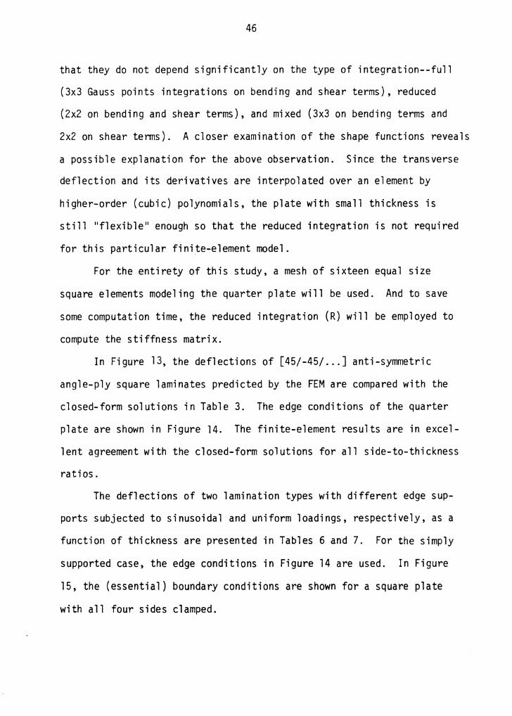
In Figure 13, the deflections of [45/-45/ ... ] anti-symmetric

angle-ply square laminates predicted by the FEM are compared with the

closed-form solutions in Table 3. The edge conditions of the quarter

plate are shown in Figure 14. The finite-element results are in excel-

lent agreement with the closed-form solutions for all side-to-thickness

ratios.

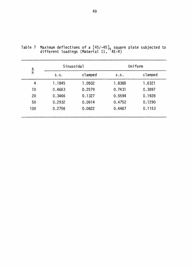
The deflections of two lamination types with different edge sup-

ports subjected to sinusoidal and uniform loadings, respectively, as a

function of thickness are presented in Tables 6 and 7. For the simply

supported case, the edge conditions in Figure 14 are used. In Figure

15, the (essential) boundary conditions are shown for a square plate

with all four sides clamped.

-w

l. 3

l.O

0.5 \

\""'-- . -- -

e FEM (4E-2x2)

CFS (n=2)

CFS (n=6)

- - ------+----

0 '--~~~~~~t--~~~~~~---~~~~~~+--~~~~~~~~~~~~~--~~~-0 10 20 :J) 40 50

a/h

Figure 13. A comparison of maximum deflections of square [45/-45/ ... ] anti-symmetric angle-ply plates subjected to sinusoidal loading (Material II).

~

"

48

Table 6 Maximum deflections of a [0/±45/90Js square plate subjected to different loadings (Material II, 4E-R)

a Sinusoidal Uniform h clamped clamped s .s. S.S.

4 l . 0837 0. 9772 l .6340 l .4648 10 0.3818 0.2615 0.5904 0.3890 20 0.2758 0 .1292 0.4336 0.1864 50 0.2435 0.0798 0.3859 0. 1108

100 0.2375 0.0699 0.3769 0.0960

49

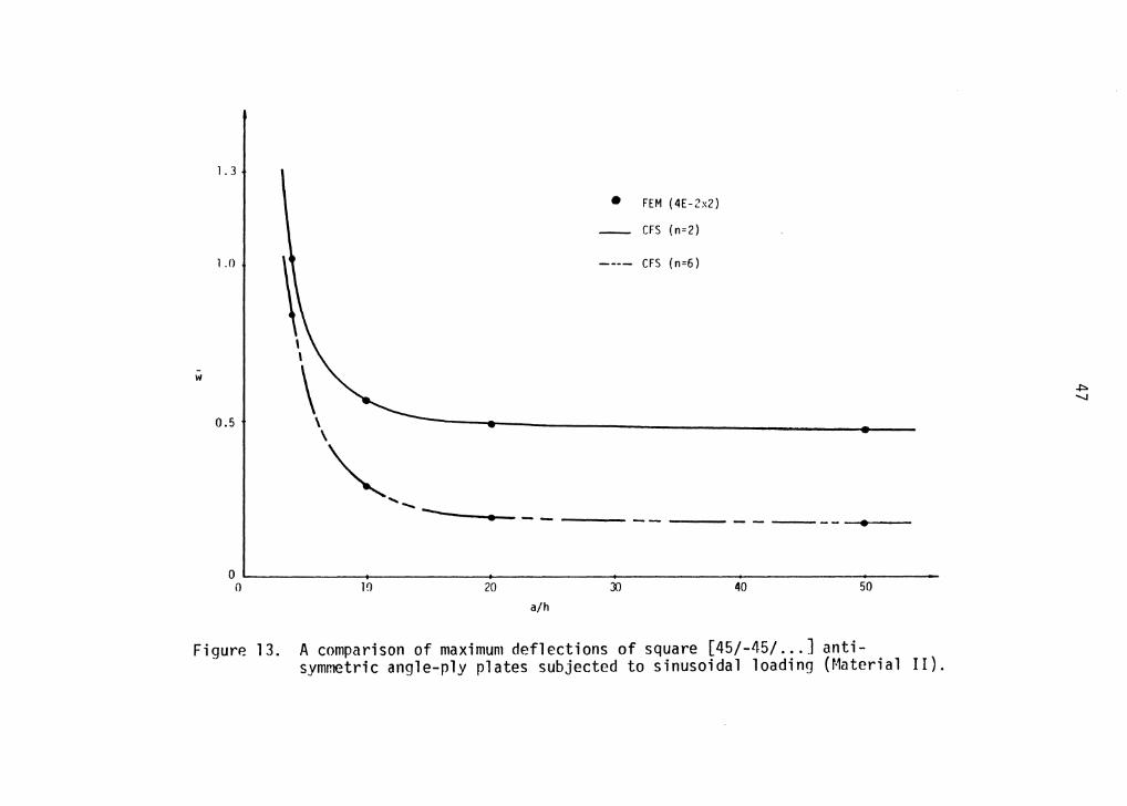
Table 7 Maximum deflections of a [45/-45Js square plate subjected to different loadings (Material II, 4E-R)

a Sinusoidal Uniform h s .s. clamped s .s. clamped

4 1 .1845 l .0502 1.8385 1 . 6321 10 0.4663 0.2579 0.7431 0.3897 20 0.3466 0 .1327 0.5594 0 .1928 50 0.2932 0.0914 0.4752 0 .1290

100 0.2756 0.0822 0.4467 0.1153

50

y

v ,w' r./J = 0 x -, I I

u ,w' r./J y = 0

I I I

Figure 14 Boundary conditions for a simply supported (S-2) quarter plate.

51

y

u,v,w, r/;x' t/Jy = 0

v w ·'· = 0 ' 'x ''fix u 'v ,w' rj; x' rj; y = 0

x

I Figure 15 Boundary conditions for plate with all edges clamped.

52

3.2 Free Vibration Analysis

For all problems discussed in this section, material II is used.

Closed-form solutions for the fundamental frequencies as a function of

side-to-thickness ratios are presented fa~ the following laminates:

l. Four-layer [0/90/90/0] symmetric cross-ply square plate.

2. Two- and six-layer [0/90/ ... ] anti-symmetric cross-ply square

plates.

3. Two- and six-layer [8/-8/ ... ] anti-symmetric angle-ply square

plates with e = 5°, 30° and 45°.

The (S-1) type of simply supported edge conditions is employed for the

cross-ply plates, and the (S-2) type is specified for the angle-ply

laminates. Note that the rotary inertias are included in all three

theories. Table 8 contains the non-dimensionalized fundamental fre-

quencies of the cross-ply [0/90/90/0] laminated plate. From

the above results, the CPT overestimates the frequencies for all side-

to-thickness ratios. The error is as much as 100% for thick plate in

·comparison with the other two theories. On the other hand, the HSDT is

in excellent agreement with the FSDT (see Reddy and Chao [17]).

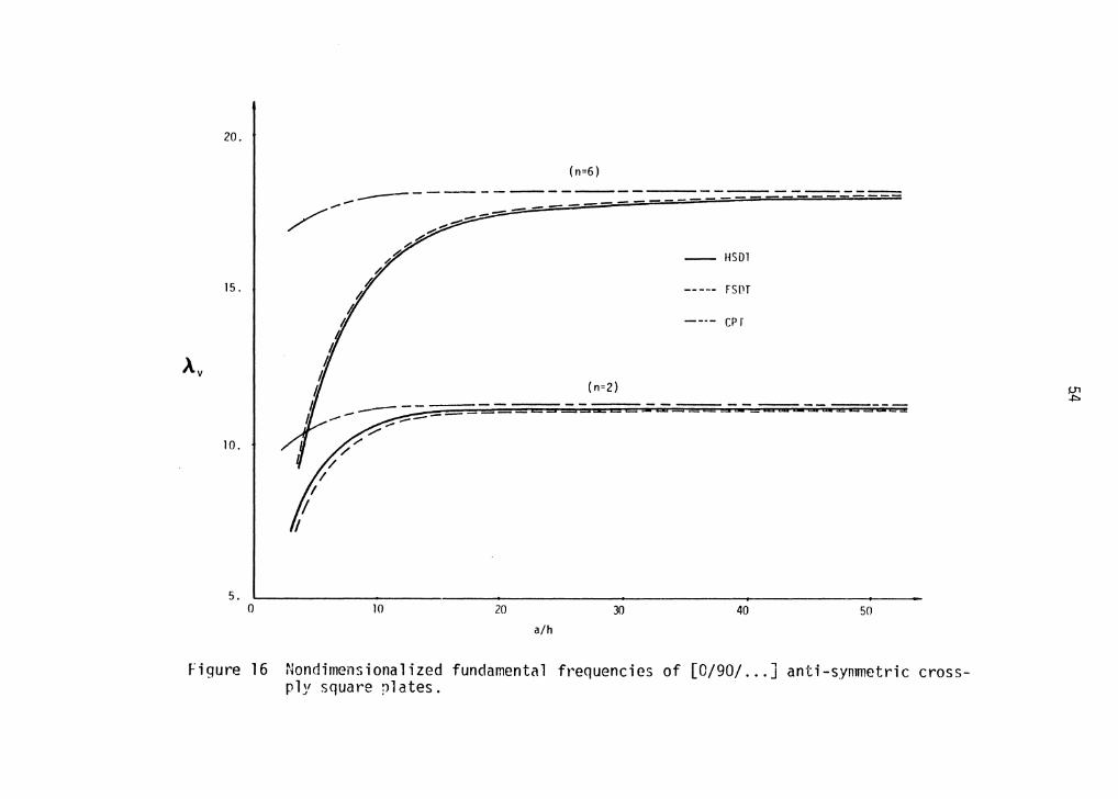
The fundamental natural frequencies of the anti-syrrnnetric cross-ply

[0/90/ ... ] case are shown in Figure 16. The plots show that the shear

deformation effect is more dominant on the behavior of plates with the

decrease in bending-stretching coupling. The above phenomenon is also

observed in the case of anti-symmetric angle-ply laminates (see Table 9).

As a result, the effects of shear deformation and coupling must be con-

sidered simultaneously.

53

Table 8 Non-dimensionalized fundamental frequencies+of a [0/90/90/0] square plate

a CPT FSDT [17] HSDT h

4 17.989 9.395 9.324

10 18.738 15. 143 15. 107

20 18. 853 17.660 17. 647

50 18.885 18.674 18.672

100 18.890 18. 836 18. 836

20.

/----------------(n=6) ----~=-=--:...=-===-=-'=-==-= -~~~

-- HSDl

15. FSOT

CP f

Av (n=2)

----- ....... =----

10.

5. 0 10 20 30 40 50

a/h

Figure 16 Nondimensionalized fundament~l frequencies of [0/90/ ... ] anti-syn~etric cross-ply square plates.

~

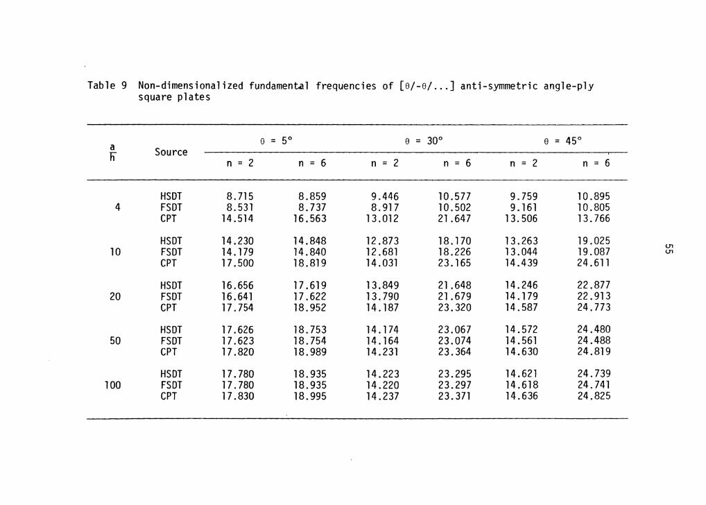
Table 9 Non-dimensionalized fundamental frequencies of [e/-e/ ... ] anti-symmetric angle-ply square plates

0 = 5° e = 30° e = 45° a Source h n = 2 n = 6 n = 2 n = 6 n = 2 n = 6

HSDT 8.715 8.859 9.446 10.577 9.759 10.895 4 FSDT 8.531 8. 737 8.917 10. 502 9. 161 10.805

CPT 14.514 16.563 13. 012 21 .647 13.506 13.766

HSDT 14.230 14.848 12.873 18. 170 13.263 19.025 10 FSDT 14. 179 14.840 12. 681 18. 226 13.044 19.087

CPT 17 .500 18.819 14. 031 23.165 14.439 24.611

HSDT 16.656 17.619 13.849 21 .648 14.246 22 .877 20 FSDT 16. 641 17.622 13. 790 21.679 14. 179 22.913

CPT 17.754 18.952 14 .187 23.320 14.587 24. 773

HSDT 17.626 18.753 14. 174 23.067 14.572 24.480 50 FSDT 17.623 18.754 14. 164 23.074 14.561 24.488

CPT 17.820 18.989 14. 231 23.364 14.630 24.819

HSDT 17. 780 18. 935 14.223 23.295 14.621 24.739 100 FSDT 17.780 18.935 14.220 23.297 14.618 24.741

CPT 17.830 18.995 14.237 23.371 14.636 24.825

tn tn

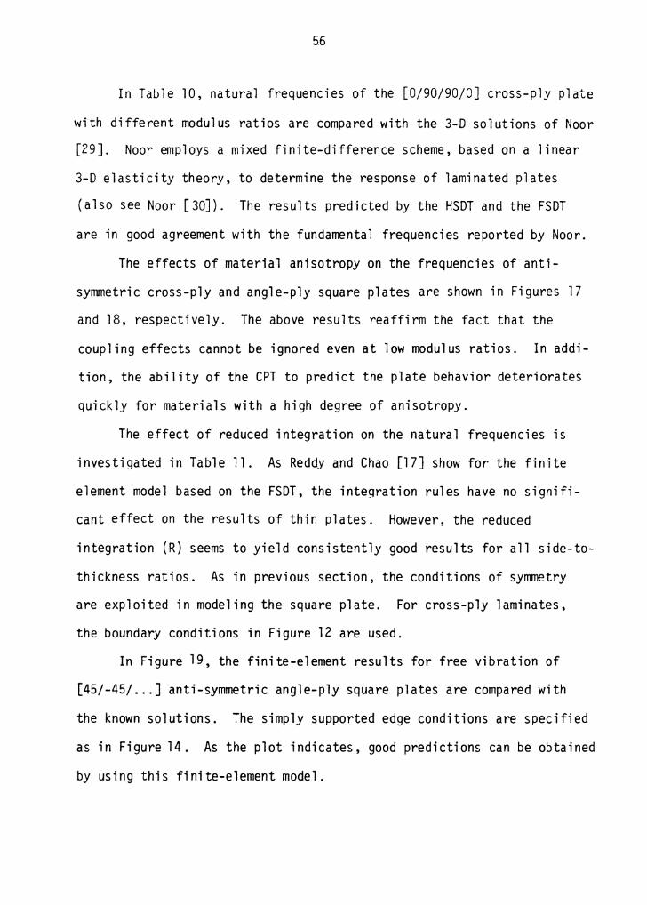
In Table 10, natural frequencies of the [0/90/90/0] cross-ply plate

with different modulus ratios are compared with the 3-D solutions of Noor

[29]. Noor employs a mixed finite-difference scheme, based on a linear

3-0 elasticity theory, to determine the response of laminated plates

(also see Noor [30]). The results predicted by the HSDT and the FSDT

are in good agreement with the fundamental frequencies reported by Noor.

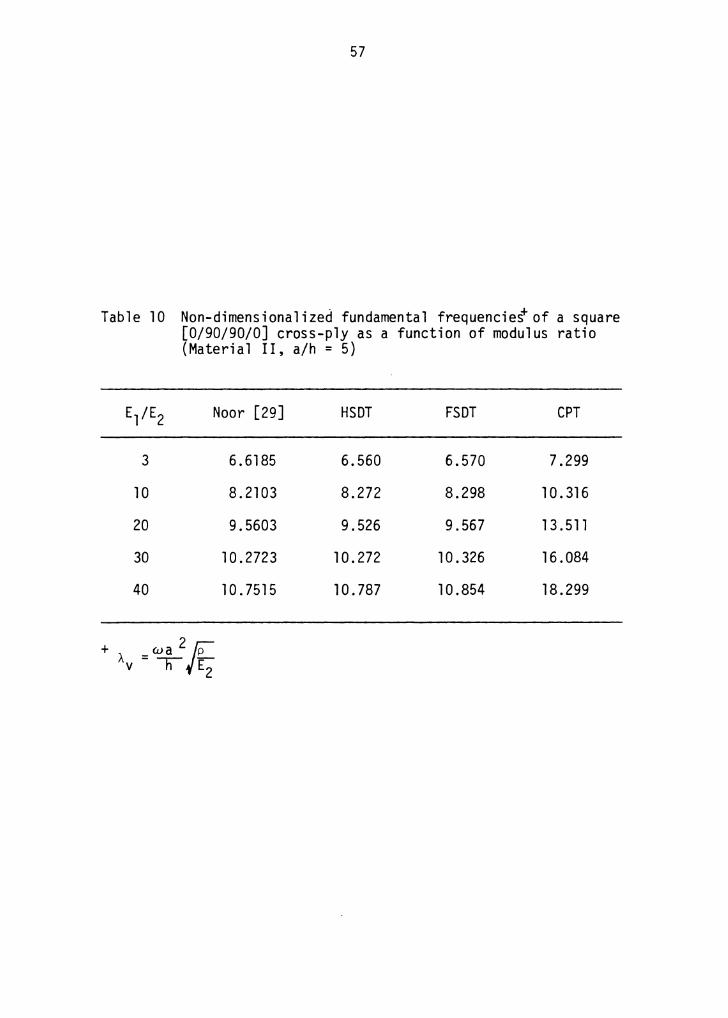
The effects of material anisotropy on the frequencies of anti-

symmetric cross-ply and angle-ply square plates are shown in Figures 17

and 18, respectively. The above results reaffirm the fact that the

coupling effects cannot be ignored even at low modulus ratios. In addi-

tion, the ability of the CPT to predict the plate behavior deteriorates

quickly for materials with a high degree of anisotropy.

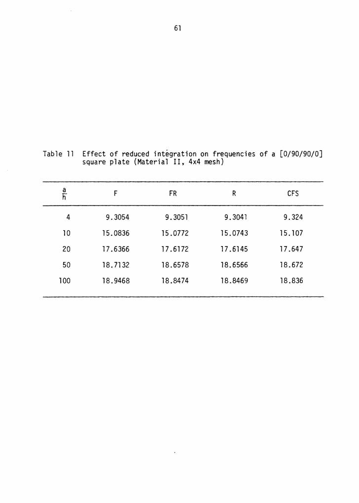
The effect of reduced integration on the natural frequencies is

investigated in Table 11. As Reddy and Chao [17] show for the finite

element model based on the FSDT, the inte~ration rules have no signifi-

cant effect on the results of thin plates. However, the reduced

integration (R) seems to yield consistently good results for all side-to-

thickness ratios. As in previous section, the conditions of symmetry

are exploited in modeling the square plate. For cross-ply laminates,

the boundary conditions in Figure 12 are used.

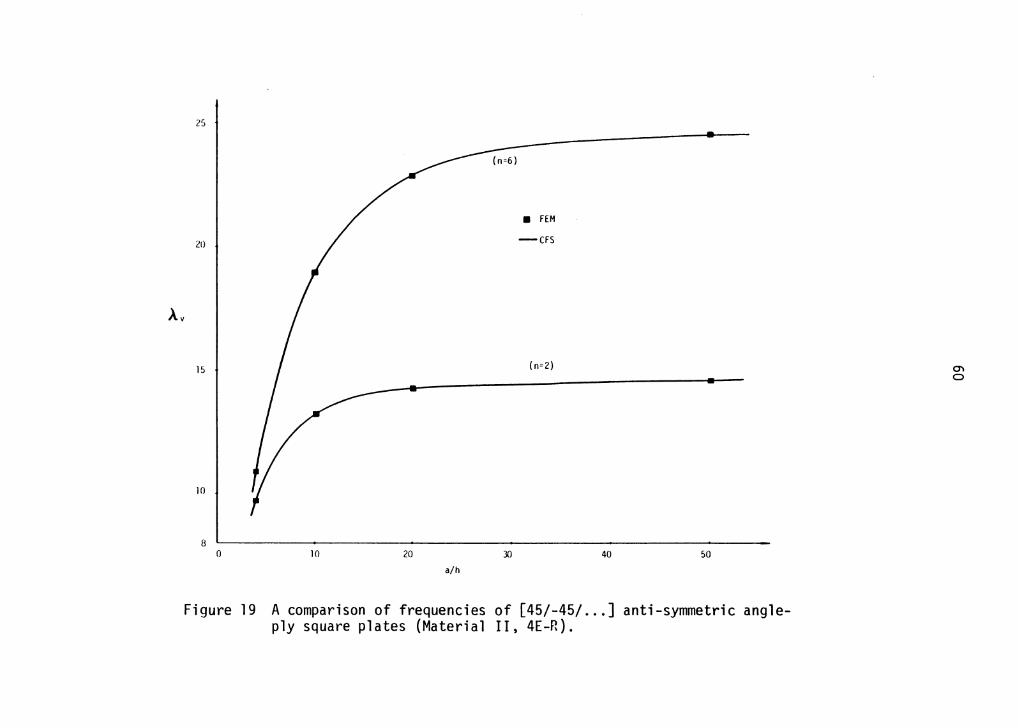
In Figure 19, the finite-element results for free vibration of

[45/-45/ ... ] anti-symmetric angle-ply square plates are compared with

the known solutions. The simply supported edge conditions are specified

as in Figure 14. As the plot indicates, good predictions can be obtained

by using this finite-element model.

57

Table 10 Non-dimensionalized fundamental frequencies+ of a square [0/90/90/0] cross-ply as a function of modulus ratio (Material II, a/h = 5)

E1/E2 Noor [29] HSDT FSDT CPT

3 6.6185 6.560 6.570 7.299

10 8. 2103 8.272 8.298 10.316

20 9.5603 9.526 9.567 13.511

30 10. 2723 10.272 10. 326 16.084

40 10.7515 10.787 10.854 18.299

58

20. • Noor

-- HSDT

----- FSDT

--- CPT / ./ ,,

15. / / ,,,.

/ A. v

/ / (n:z6) / • /

/

1 a. /

Figure 17 Effect of material anisotropic on the frequencies of [0/90/ ••. ] anti-symmetric cross-ply square plates (a/h = 5).

59

25 / , , HSDT /

"' "' FSDT /

/ /

CPT / /

/

20 / / (n=6)

/

/ /

/

I 15

A.v -----------(n=2)

10

5 0 10 20 30

Figure 18 Effect of material anisotropy on the frequencies of [45/-45/ ... J anti-syrmnetric angle-ply square plates (a/h = 10).

40

A.v

25

• FEM

20 -CFS

15 (n=2)

JO

8 0 JO 20 30 40 50

a/h

Figure 19 A comparison of frequencies of [45/-45/ ... ] anti-symmetric angle-ply square plates (Material II, 4E-R).

O'I 0

61

Table 11 Effect of reduced integration on frequencies of a [0/90/90/0] square plate (Material II, 4x4 mesh)

a F FR R CFS h

4 9.3054 9. 3051 9. 3041 9.324

10 15.0836 15 .0772 15.0743 15. 107

20 17.6366 17.6172 17.6145 17.647

50 18. 7132 18.6578 18.6566 18. 672

100 18.9468 18.8474 18.8469 18.836

62

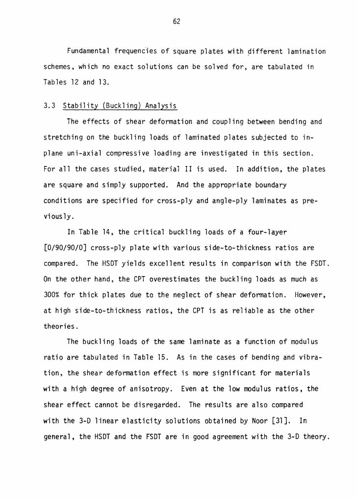
Fundamental frequencies of square plates with pifferent lamination

schemes, which no exact solutions can be solved for, are tabulated in

Tables 12 and 13.

3.3 Stability (Buckling) Analysis

The effects of shear deformation and coupling between bending and

stretching on the buckling loads of laminated plates subjected to in-

plane uni-axial compressive loading are investigated in this section.

For all the cases studied, material II is used. In addition, the plates

are square and simply supported. And the appropriate boundary

conditions are specified for cross-ply and angle-ply laminates as pre-

viously.

In Table 14, the critical buckling loads of a four-layer

[0/90/90/0] cross-ply plate with various side-to-thickness ratios are

compared. The HSDT yields excellent results in comparison with the FSDT.

On the other hand, the CPT overestimates the buckling loads as much as

300% for thick plates due to the neglect of shear defonnation. However,

at high side-to-thickness ratios, the CPT is as reliable as the other

theories.

The buckling loads of the same laminate as a function of modulus

ratio are tabulated in Table 15. As in the cases of bending and vibra-

tion, the shear deformation effect is more significant for materials

with a high degree of anisotropy. Even at the low modulus ratios, the

shear effect cannot be disregarded. The results are also compared

with the 3-D linear elasticity solutions obtained by Noor [31]. In

general, the HSDT and the FSDT are in good agreement with the 3-D theory.

63

Table 12 Nondimensionalized frequencies of a [45/-45Js square plate with different boundary conditions (Material II, 4E-R)

a Simply supported Clamped h

4 9. 1455 9.7457

10 14.6261 20.3486

20 17. 1094 29.5478

50 J8.6081 36.3767

100 19. 1435 38.3979

64

Table 13 Nondimensionalized frequencies of a [0/±45/90Js square plate with different boundary conditions (Material II, 4E-R)

a Simply supported Clamped h

4 9.5661 10.1593

10 16. 1928 20.0915

20 19.0997 29.4976

50 20.3226 38.5533

100 20. 5591 41 .4066

65

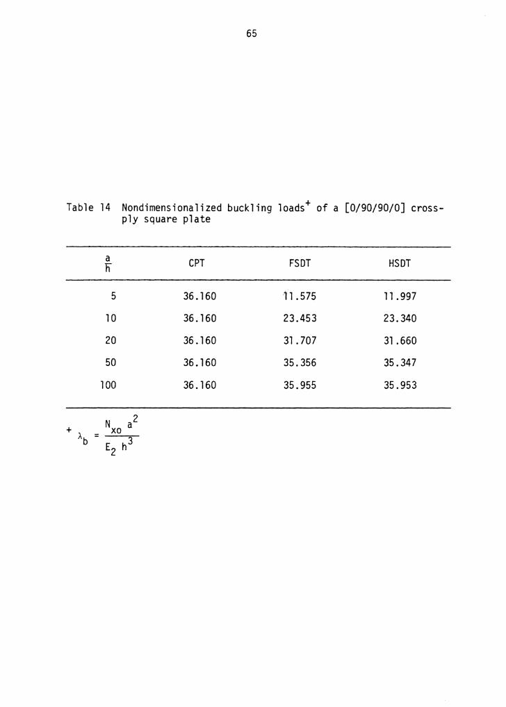
Table 14 Nondimensionalized buckling loads+ of a [0/90/90/0] cross-ply square plate

a CPT FSDT HSDT h

5 36. 160 '11.575 11. 997

10 36. 160 23.453 23.340

20 36. 160 31 .707 31 .660

50 36. 160 35.356 35.347

100 36. 160 35.955 35.953

+ N a2 A = XO b E h3

2

66

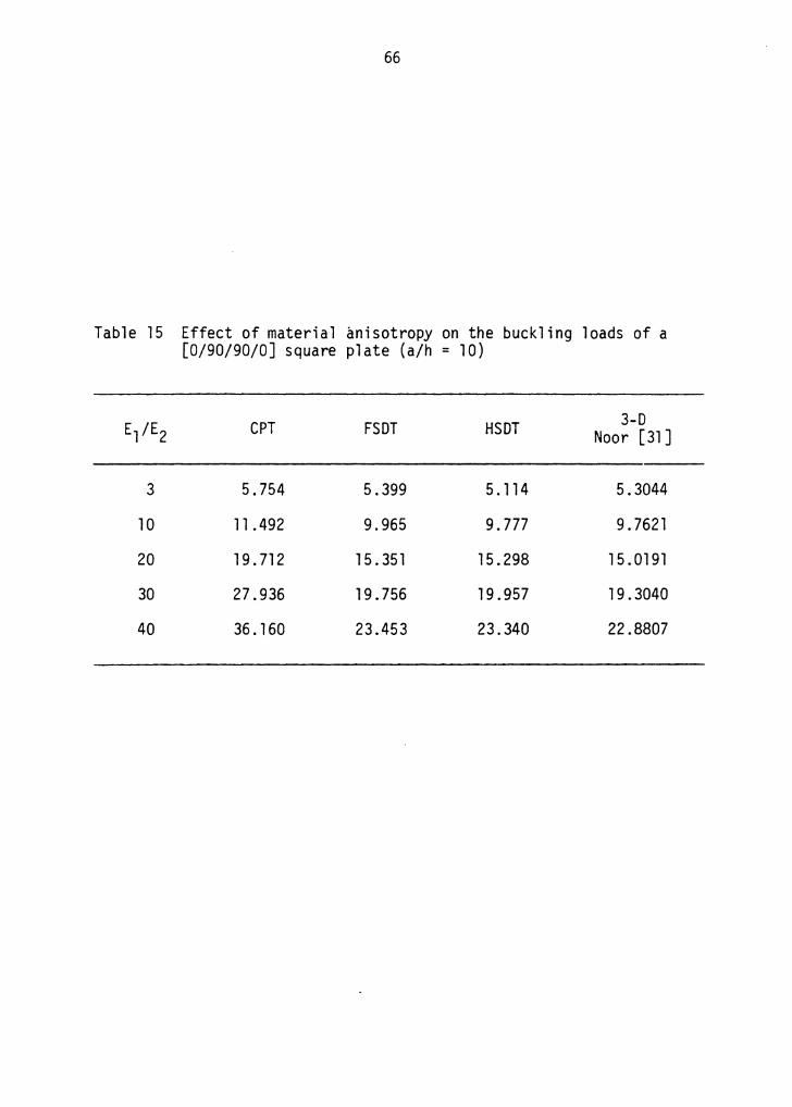
Table 15 Effect of material anisotropy on the buckling loads of a [0/90/90/0] square plate (a/h = 10)

E1/E2 CPT FSDT HSDT 3-D Noor [31]

3 5.754 5.399 5.114 5.3044

10 11 . 492 9.965 9. 777 9.7621

20 19.712 15. 351 15.298 15.0191

30 27.936 19.756 19.957 19.3040

40 36. 160 23.453 23.340 22.8807

67

Note that.Noor employs a finite-difference scheme to solve for solutions

of the governing equations, hence his results are not exact.

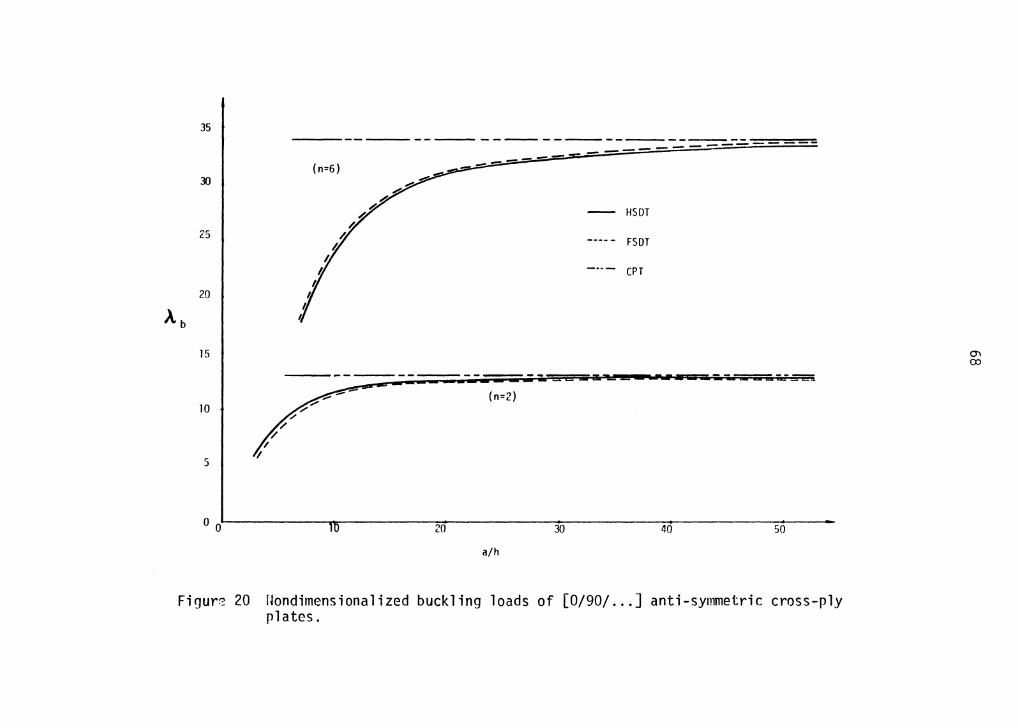
In Figure 20, the buckling loads of two- and six-layer [0/90/ ... ]

anti-sy1T111etric cross-ply laminates are shown. Consistent with the

earlier observations, the shear effect is less pronounced for the two-

layer cross-ply plates than for the six-layer plates. As a result, the

coupling between bending and stretching must be taken into account in

considering the effect of shear deformation on the gross response

(buckling loads in this case) of the plate. As in the case of cross-ply,

Table 16 shows that the shear effect is most severe for the six-layer

anti-symmetric angle-ply laminate with e = 5° at a given thickness.

The buckling loads as a function of modulus ratio of anti-symmetric

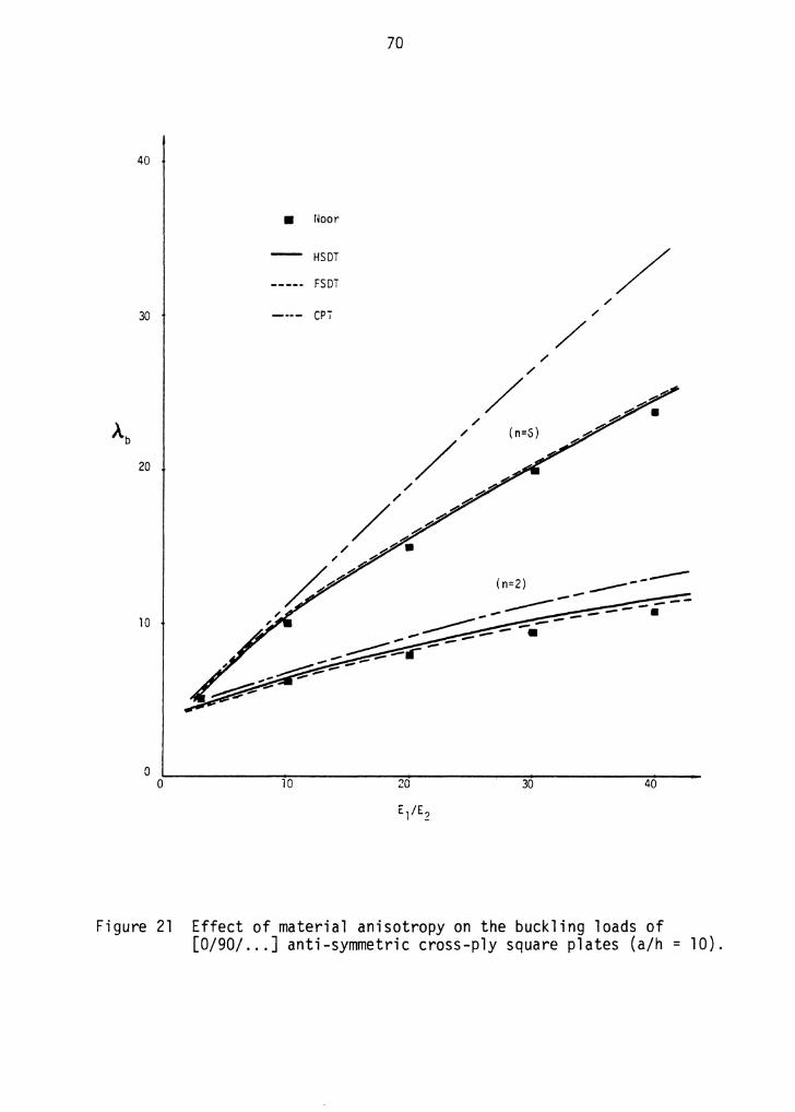
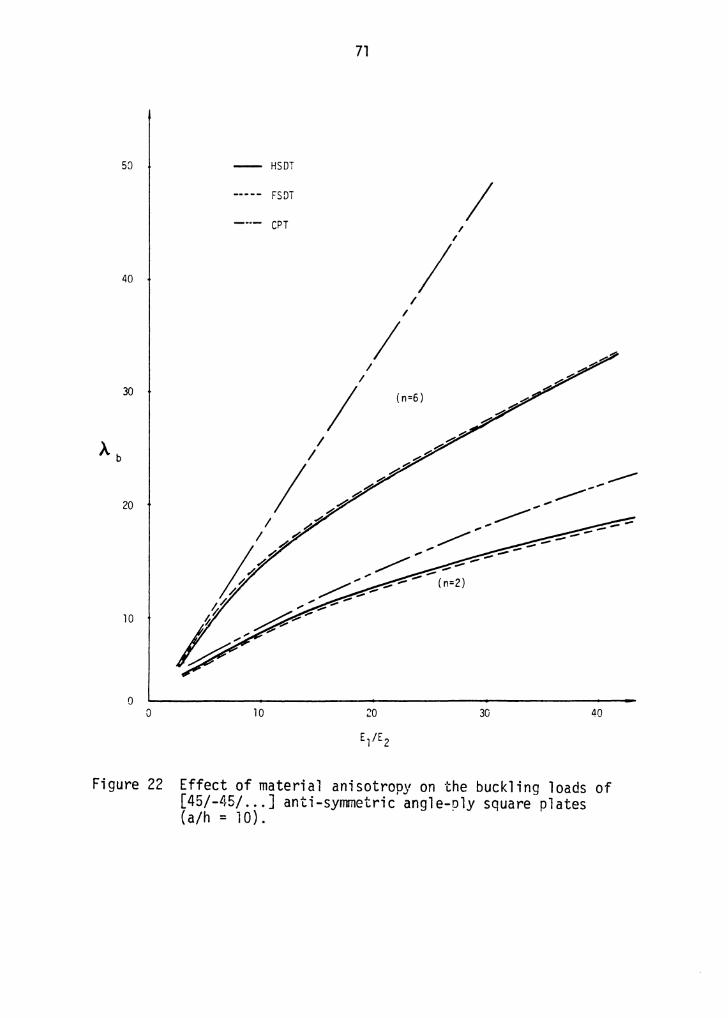
cross-ply and angle-ply are plotted in Figures 21-22, respectively. As

confirmed by other investigators, the coupling effect on the buckling

loads is more pronounced with the increasing degree of anisotropy.

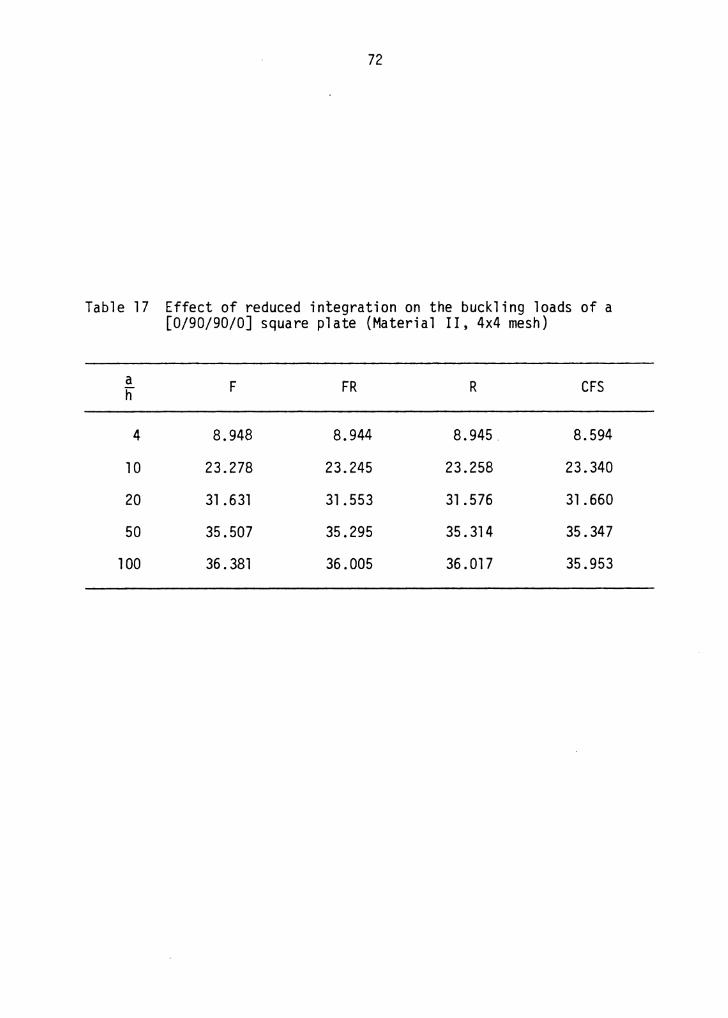
Using the finite-element model introduced in previous chapter,

the effects of reduced integration on the buckling loads of the

[0/90/90/0] cross-ply laminate is investigated. As shown in Table 17,

the type of integration rule again has no significant effect on the

buckling loads.

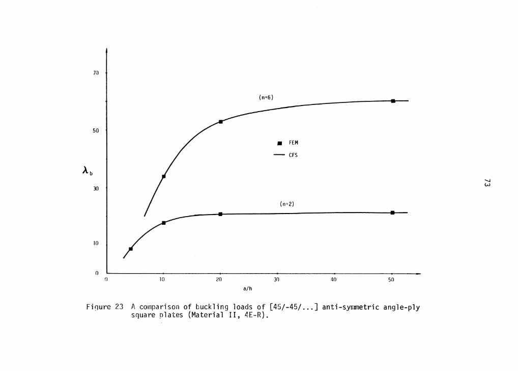
In Figure 23, the buckling loads of [45/-45/ ... ] anti-symmetric

angle-ply plates obtained from the finite-element model are compared

with the closed-form solutions from Table 16. The accuracy of the

finite-element model can be seen from the above figure.

68

>. ...... c...

I I Vl

I V

l I

0 0

~

I L

() u

I u

..... •I

~

.;....> '1

QJ

I~ § >, V

l I

I .....

0 ..µ

I ""

c::: re I

,_ ,_

0 0

,_ r-i

I V

l V

l 0..

::i:: u..

u

I .........

I 0 O'> ......... 0 1

--l

I 4

-I

0

I V

l "'O

\

~

re C

'J II

..r::: 0

\ c:

...... ......

\ "'

Ol

1 c:::

..... ...... 0

~

~ C

J u :::I

~ ..0

~ "'O

~

ClJ N

~

.,... ~

...... 'II

re c::: 'il

0 ...;:

..... "'

-.;:: (/)

" ...

c::: c:

-.;: <lJ E

V

l .....

CJ "'O

..µ c:::

re 0

...... =

0..

0 N

0 ('.' ~

I.fl '"

0 "'

0 L

'") 0

:::I M

'"

N

I::"> .....

.D

L.l...

--<

69

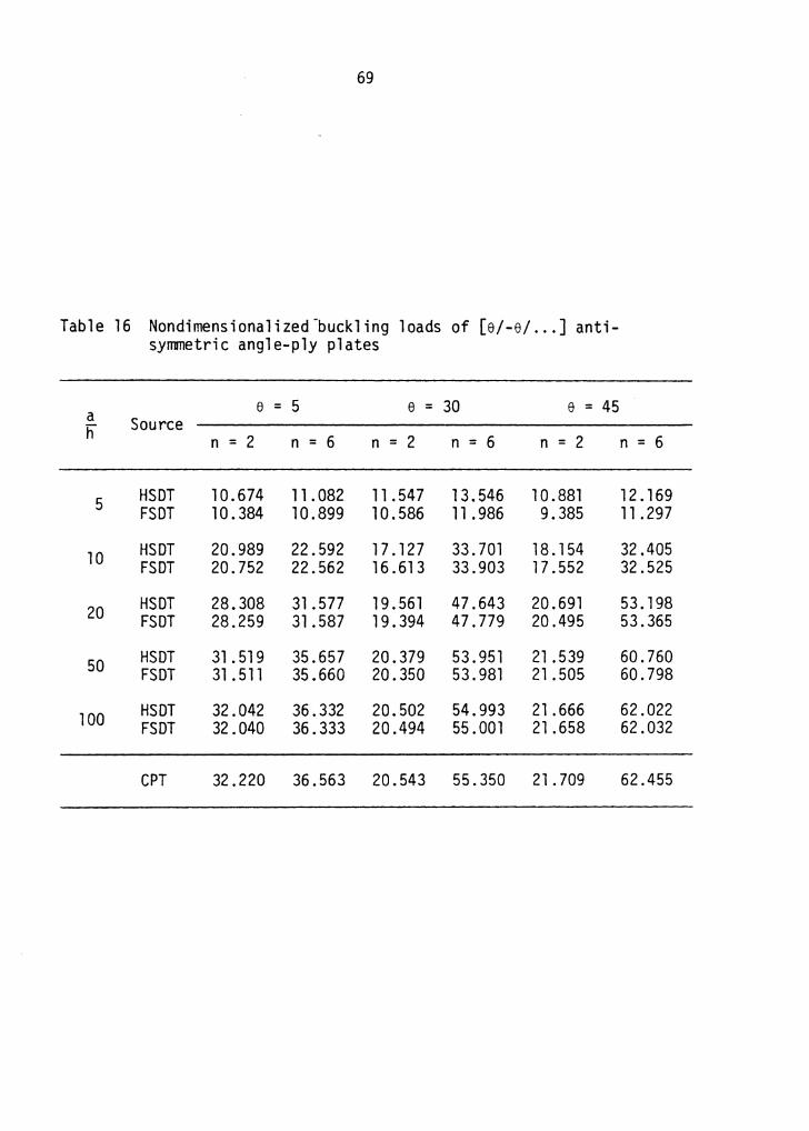
Table 16 Nondimensionalized-buckling loads of [e/-e/ ... ] anti-symmetric angle-ply plates

a e = 5 e = 30 e = 45 h Source

n = 2 n = 6 n = 2 n = 6 n = 2

5 HSDT 10.674 11. 082 11. 547 13.546 10 .881 FSDT 10. 384 10.899 10.586 11. 986 9.385

10 HSDT 20.989 22.592 17. 127 33.701 18. 154 FSDT 20.752 22.562 16.613 33.903 17.552

20 HSDT 28.308 31 .577 19. 561 47.643 20.691 FSDT 28.259 31.587 19.394 47. 779 20.495

50 HSDT 31 . 519 35.657 20.379 53.951 21 .539 FSDT 31. 511 35.660 20.350 53. 981 21.505

100 HSDT 32.042 36.332 20.502 54.993 21.666 FSDT 32 .040 36.333 20.494 55.001 21.658

CPT 32.220 36.563 20.543 55.350 21.709

n = 6

12 .169 11 . 297

32.405 32.525

53.198 53.365

60.760 60.798

62.022 62.032

62.455

70

40

• Noor

HSDT / FSDT /

30 CPi /

/ /

/

/ ,<[; • / ..id

Ab / (n=S)

/ 20 /

/

/ A. .6

/ ..i;'°' •

(n=2)

10

0 0 10 20 30 40

Figure 21 Effect of material anisotropy on the buckling loads of [0/90/ ... ] anti-symmetric cross-ply square plates (a/h = 10).

50

40

30

20

10

0

-- HSDT

FSDi

CPT

I

10

I I

71

I I

I

I I

I I

20

{n=6)

, , I

30 40

Figure 22 Effect of material anisotropy on the buckling loads of (45/-45/ ... ] anti-symmetric angle-ply square plates {a/h = 10).

72

Table 17 Effect of reduced integration on the buckling loads of a [0/90/90/0] square plate (Material II, 4x4 mesh)

a F FR R CFS h

4 8.948 8.944 8. 945. 8.594

10 23.278 23.245 23.258 23.340

20 31 .631 31.553 31 .576 31.660

50 35.507 35.295 35.314 35.347

l 00 36. 381 36.005 36.017 35.953

70

(n=6)

50 I / • FEM

- CFS t /

A.b I •

30

t I (n=2)

10

0 !) 10 20 30 40 50

a/h

Fi~ure 23 A comparison of buckling loads of [45/-45/ ... ] anti-syl'ilTletric angle-ply square plates (Material II, 4E-R).

--.J w

74

The buckling loads of a [45/-45]s symmetric angle-ply laminate

and a [0/±45/90]s quasi-isotropic laminate with different edge conditions

are shown in Tables 18-19, respectively.

75

Table 18 Nondimensionalized buckling loads of a [45/-45]~ square plate with different boundary conditions (Material II, 4E-R)

a Simply-supported Clamped-clamped h

4 7.2587 7.4099

10 21 .1248 31 .0778

20 29.1504 67.7942

50 34.5962 l 02 .1070

100 36.6451 113.4310

76

Table 19 Nondimensionalized buckling loads of a [0/±45/90]5 square plate with different boundary conditions (Material II, 4E-R)

a Simply-supported Clamped-clamped h

4 9.3323 10 .1459

10 26.7994 39.7451

20 37.1151 83.7968

50 41.8769 123.5550

100 42.8192 135. 7250

4.1 Summary

CHAPTER IV

SUMMARY AND CONCLUSION

A higher-order shear deformation theory (HSDT) suggested by Reddy

[4] is used to analyze laminated composite plates for bending, free

vibrations, and buckling. For plates with special lamination

schemes and specific boundary conditions, closed-form results are ob-

tained and compared with other displacement theories and 3-D elasticity

solutions. A finite element model is also developed to analyze plates

with arbitrary boundary conditions.

The effects of shear deformation, coupling between bending and ex-

tension, and material anisotropy on the response of laminate

composite plates are investigated. The results for some commonly used

laminates are presented to serve as references for future investigators.

4.2 Conclusion

Overall, the higher-order shear deformation theory (HSDT) gives, in

general, more accurate solutions than the classical plate theory and the

first-order shear deformation theory. Even though the displacements vary

cubically through the thickness of the plate, the HSDT contains the same

number of dependent unknowns as the FSDT. The theory yields a parabolic

distribution of the transverse shear stresses through the thickness, and

free-stress boundary conditions on top and bottom surfaces of the plate

are satisfied.

77

78

In the present study, the effects of coupling and material

anisotropy on the response of plates are confirmed with other in-

vestigators' findings. It is also found that the FSDT overpredicts the

deflections, and underestimates the natural frequencies and buckling

loads for medium to thick anti-symmetric cross-ply and angle-ply plates

as a result of the imprecise determination of the shear correction co-

efficients. Therefore, the HSDT provides a better theory for the

analysis of laminated composite plates.

REFERENCES

[l] Yang, P. C., Norris, C.H. and Stavsky, Y., 11 Elastic Wave Propagation in Heterogeneous Plates, 11 Int. J. of Solids and Structures, Vol. 2, pp. 665-684, October 1966.

[2] Whitney, J.M., Pagano, N. J., 11 Shear Defonnation in Heterogeneous Anisotropic Plates, 11 J. Applied Mechanics, Vol. 37, pp. 1031-1036, December 1970.

[3] Lo, K. H., Christensen, R. M. and Wu, E. M., 11A Higher-Order Theory of Plate Defonnation, Part 2: Laminated Plates, 11 J. Applied Mechanics, Vol. 44, No. 4, pp. 669-676, December 1977.

[4] Reddy, J. N., 11 A Simple Higher-Order Theory for Laminated Composite Plates, 11 Report VPI-E-83.28, ESM Department, Virginia Polytechnic Institute, Blacksburg, VA, June 1983.

[5] Reissner, E., "The Effect of Transverse Shear Deformation on the Bending of Elastic Plates, 11 J. Appl. Mech., Vol. 12, No. 2, pp. 69-77, June 1945 .

[6] Hencky, H., 11 Uber die Berucksichtigung der Schubverzerrungen in Eben Platten, 11 Ing.-Arch., Vol. 16, 1947.

[7] Mindlin, R. D., 11 Influence of Rotary Inertia and Shear on Flexural Motions of Isotropic Elastic Plates, 11 J. Appl. Mech., Vol. 18, No. 1, pp. 31-38, March 1951.

[8] Stavsky, Y. , 110n the Theory of Symmetrical Heterogeneous Pl ates Having the Same Thickness Variation of the Elastic Moduli , 11 Topics in Applied Mechanics, Ed. by Abir, D., Ollendorff, F. and Reiner, M., American Elsevier, New York, 1965.

[9] Whitney, J.M. and Sun, C. T., 11A Higher Order Theory for Exten-sional Motion of Laminated Composites, 11 J. Sound and Vibration, Vol. 30, pp. 85-97, September 1973.

[10] Levinson, M., 11 An Accurate, Simple Theory of the Statics and Dynamics of Elastic Plates, 11 Mechanics Research Communications, Vol. 7, No. 6, pp. 343-350, 1980.

[11] Murthy, M. V. V., "An Improved Transverse Shear Deformation Theory for Laminated Anisotropic Plates, 11 NASA Technical Paper 1903, November 1981 .

79

80

[12] Pryor, Jr., C. W. and Barker, R. M., "A Finite Element Analysis Including Transverse Shear Effects for Applications to Laminated Plates," AIAA Journal, Vol. 9, pp. 912-917, 1971.

[13] Mau, S. T., Tong, P. and Pian, T. H. H., "Finite Element Solutions for Laminated Thick Plates, 11 J. Composite Materials, Vol. 6, pp. 304-311 ' 1972.

[14] Mau, S. T. and Witmer, E. A., "Static, Vibration and Thennal Stress Analyses of Laminated Plates and Shells by the Hybrid-Stress Finite Element Method with Transverse Shear Deformation Effects Included, 11 Aeroelastic and Structures Research Laboratory, Report ASRL TR 169-2, Department of Aeronautics and Astronautics, MIT, Cambridge, MA, 1972.

[15] Noor, A. K. and Mathers, M. D., "Anisotropy and Shear Deformation in Laminated Composite Plates," AIAA Journal, Vol. 14, pp. 282-285, 1976.

[16] Noor, A. K. and Mathers, M. D., "Finite Element Analysis of Anisotropic Plates," Int. J. Num. Meth. Engng., Vol. 11, pp. 289-307, 1977.

[17] Reddy, J. N. and Chao, W. C., "A Comparison of Closed-Form and Finite Element Solutions of Thick Laminated Anisotropic Rectangular Plates," Nuclear Engineering and Design, Vol. 64, pp. 153-167, 1981.

[18] Reddy, J. N., 11A Penalty Plate-Bending Element for the Analysis of Laminated Anisotropic Composite Plates," Int. J. Num. Meth. Engng., Vol . 15, pp. 1187-1206, 1980.

[19] Reddy, J. N., "Free Vibration of Antisymmetric, Angle-ply Laminated Plates, Including Transverse Shear Deformation by the Finite Element Method, 11 J. Sound and Vibration, Vol. 66, No. 4, pp. 565-576, 1979.

[20] Reddy, J. N. and Rasmussen, M. L., Advanced Engineering Analysis, Wiley & Son, 1982.

[21] Reddy, J. N., An Introduction to the Finite Element Method, McGraw-Hill, 1984.

[22] Zienkiewicz, 0. C., The Finite Element Method, McGraw-Hill, 1977.

[23] Pagano, N. J. and Hatfield, S. J., "Elastic Behavior of Multi-layered Bidirectional Composites," AIAA Journal, Vol. 10, pp. 931-933, July 1972.

[24] Whitney, J. M., "The Effect of Transverse Shear Deformation on the Bending of Laminated Plates, 11 J. of Composite Materials, Vol. 3, No. 3, July 1969, pp. 534-547.

81

[25] Whitney, J. M. , "Shear Correction Factors for Orthotropi c Laminates Under Static Load, 11 J. Appl. Mech., Vol. 40, pp. 302-304, March 1973.

[26] Chow, T. S., "On the Propagation of Flexural Waves in an Ortho-tropic Laminated Plate and Its Response to an Impulsive Load, 11

J. Composite Materials, Vol. 5, No. 3, pp. 306-319, July 1971.

[27] Noor, A. K. and Mathers, M. D., 11 Anisotropy and Shear Deformation in Laminated Composite Plates," AIAA Journal, Vol. 14, No. 2, pp. 282-285, February 1976.

[28] Whitney, J. M. , 11 Bend i ng-Extens i ona l Coup 1 i ng in Laminated P 1 ates Under Transverse Loading, 11 J. Composite Materials, Vol. 3, pp. 20-28, January 1969.

[29] Noor, A. K., 11 Free Vibrations of Multi layered Composite Plates, 11

AIAA Journa 1 , Vo 1 . 11 , No. 7, pp. l 038-1039, November 1972.

[30] Noor, A. K., "Mixed Finite-Difference Scheme for Analysis of Simply Supported Thick Plates," Computers & Structures, Vol. 3, pp. 967-982, 1973.

[31] Noor, A. K., 11 Stability of Multilayered Composite Plates, 11 Fibre Science and Technology, Vol. 8, pp. 81-88, 1975.

APPENDIX A A BRIEF DERIVATION OF THE ASSUMED DISPLACEMENT FIELD

The displacements are assumed to have the following form,

u, ( x ,y ,z) = u(x,y) + z ~x(x,y) + z2 ~x(x,y) + z3 ~x(x,y)

u2(x,y,z) = v(x,y) + z ~y(x ,y) + z2 ~y(x,y) + z3 ~Y(x,y)

u3(x,y,z) = w(x,y) (A. 1)

where u, v, w denote the displacements of a point on the midplane, and

~x' ~Y are the rotations of the normals to the midplane about they-

and x-axis, respectively. The remaining unknowns (~x'~x'~y'~y) can be

determined by imposing the stress-free boundary conditions on the top

and bottom surfaces of the plate, which can be expressed analytically by

ayz(x,y,± ~) = 0 , axz(x,y,± ~) = 0 (A. 2)

The above conditions also imply, for orthotropic plates and plates lami-

nated of orthotropic layers, that the corresponding transverse shear

strains vanish on these surfaces,

(A. 3)

From the theory of elasticity, the strains can be related to the

displacements by

au1 au3 ~ + 2z ~ + 3z2 + aw e ·- 2e13 = az + ax-= ~x 5 - x x ax

au2 au3 ~ + 2z ~ + 3z2 + aw (A.4) e = 2e23 = az + ay = ~y 4 y y ay

82

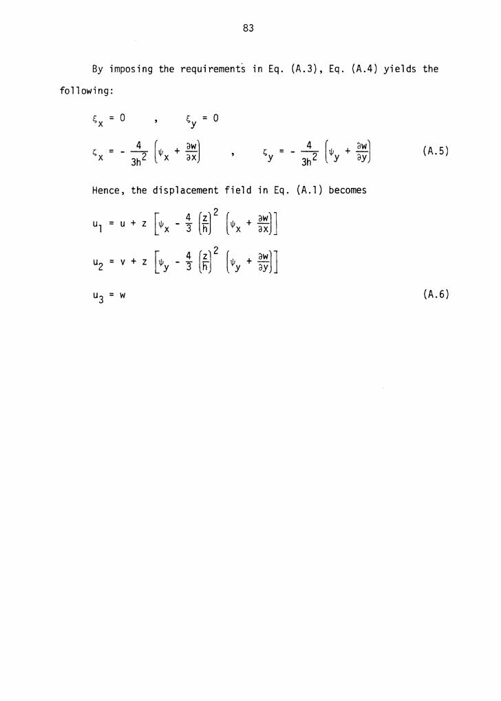
83

By imposing the requirements in Eq. (A.3), Eq. (A.4) yields the

following:

s = 0 x s = 0 y

l;; = _ ~ (ljl + aw) x 3h2 x ax l;; = _ ~ (ljl + aw~ Y 3h2 Y ayJ

Hence, the displacement field in Eq. (A.l) becomes

u 1 = u + z [ ljJ x - 4 ( ~) 2 ( ljJ x + ~~)]

u2 = v + z [ljly - t (~) 2 (ljly + ~;J]

(A. 5)

u3 = w (A.6)

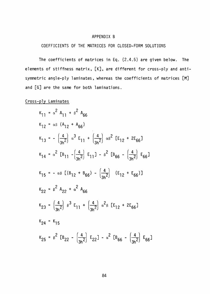
APPENDIX 8

COEFFICIENTS OF THE MATRICES FOR CLOSED-FORM SOLUTIONS

The coefficients of matrices in Eq. (2.4.5) are given below. The

elements of stiffness matrix, [K], are different for cross-ply and anti-

symmetric angle-ply laminates, whereas the coefficients of matrices [M]

and [G] are the same for both laminations.

Cross-ply Laminates

2 2 Kll = a All + S A66

Kl2 = aS (Al2 + A66)

(4) 3 (4) 2 Kl3 = - 3h2 a Ell + 3h2 aS [El2 + 2E66]

Kl 4 = a2 [81 l -(3~d Ell] - S2 [866 - (3~2] E66]

Kl5 = - aS [( 812 + 866) - (3~2] (El2 + E66)]

2 2 K22 = 8 A22 + a A66

84

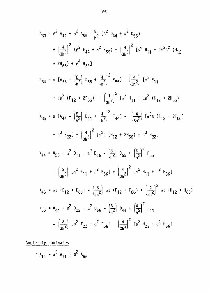
85

2 2 8 2 2 K33 = B A44 + a A55 - ~ (B D44 + a D55) h

( 4) 2 2 2 (4) 2 4 22 + 3h2 (B F44 +a F55) + 3h2 [a Hll + 2a B (Hl2

4 + 2H66) + B H22]

K34 = " [ASS - l:2J 0ss + l:l Fssl - (3:2J [a3 Fll

+ •E2 (Fl2 + 2F66)] + l3:2J2 [a3 Hll + •E2 (Hl2 + 2H66)]

3 ( 4 ) 2 2 3 + B F22J + Jh2'"J [a B (H 12 + 2H66 ) + B H22J

K44 = Ass + • 2 011 + 82 066 - (~] 0ss + l:2J2

Fss

( 8 ) 2 2 ( 4 ] 2 2 2 - 3h2J [a Fll + B F66] + 3h2 [a Hll + B H66]

K4S = •S (012 + 066) - (3:2J •S (F12 + F66) + [3:2] 2 •S (H12 + H66)

Angle-ply Laminates

vK 2 A 2 A 11 = a 11 + B 66

86

2 2 ( 4 ) 2 2 K15 = a B16 + B B26 - 3h2 [a E16 + B E26]

2 2 K22 = B A22 + a A66

2 + aB (F12

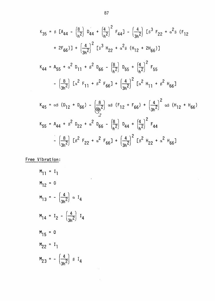
Free Vibration:

M11 = 11

M12 = 0

Ml 3 = - [3~d a 14

M15 = 0

M22 = 11

M23 = - (3~d 8 I4

87

88

M24 = 0

M2 5 = 12 - L~ d 14

2 M33 = 11 + (3~d (a2 + S2) 17

M34 = - ( 3~2) a [15 - ( 3~2) l7J

M35 = - L~2] s [15 - L;2) l7J

M45 = 0

Mss = I3 - [3~d rs + [3~2]2 I7 For angle-ply,

1 = 1 = 0 2 4

Buckling: (Nxyo = 0)

G33 = "2 + [~::] B2

G .. = 0 lJ fori,j=l,2, ... ,5 (i'!j'!3)

where Nxo and Nyo are the in-plane applied loads in the x- and y-direction,

respectively.

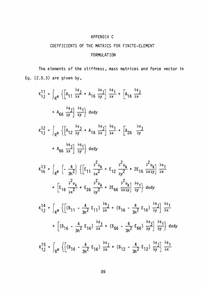
APPENDIX C

COEFFICIENTS OF THE MATRICS FOR FINITE-ELEMENT

FORMULATION

The elements of the stiffness, mass matrices and force vector in

Eq. (2.5.3) are given by,

Kl2 = I {rA acpj + A acpj] acp; + rA acpj i j Re L 12 ay 16 ax ax .L 26 ay

89

90

22 r {[ a<1>. aip .] a<1>. [ a<1>. K =j A _J+A _J_1 +A J ij Re 66 ax 26 ay ax 26 ax-

a<1> .1 a<1> .} + A22 ayJ ay, dxdy

91

[ 4 aQ>j (F66 - -2 H66) ax

3h

92

. 2 4 a<D .J a •1• } - . J o/t

+ (F26 - Jh2 H26) ay- axay dxdy

+-H --+ D --F +-H _.:....:1_ 16 J a<1>; a<1>j ~ 8 16 J a<1>; a<1> • 9h4 12 ax ay 16 3h2 16 9h4 16 ax ax

+ D - - F + H - 1 _:..J_ + D B F ~ 8 16 J a<j>. a<j> • ~ 26 2 26 --;;i- 26 66 - -2 66 3h 9h~ ay ay 3h

+ - H - 1 _J dxdy 16 ] a<j>. a<j> "}

9h4 66 ay ax .

16 ] a<1>; a<1>j ~ 8 16 ] [a<P; a<1>j + H --+ D --F +-H --9t;4 66 ax ax 26 3h2 26 9h4 26 ax ay

93

M~~ = 0 lJ

M~ 3k = - (~J J I4 <P,· ~xtJ!k dxdy l 3h.::: Re a

M~~ = 0 lJ

M~~ = 0 lJ

(3~d f Re

(3~2) f Re 4 ()tj!JI,

(I 5 - - 2 I 7) -" - cp • dxdy 3h aY J

M44 = J 03 - 82 15 + 164 I7) cp. cpJ. dxdy ij Re 3h 9h 1

M~~ = 0 1J

94

55 I a 16 M;J· = e (13 - -2 15 + -4 17) <I>·¢. dxdy R 3h 9h 1 J

G~~ = 0 lJ

where i,j = 1 ,2,3,4

£,k = 1,2,3, ... ,12

Force Vector

1 2 4 5 e F. = F. = F. = F. = p. l l l l l

r,s = 1,2,4,5 (r ~ s ~ 3)

£ = 1,2, ... ,12

i = 1,2, ... ,4

where Qe and P~ are the internal nodal forces of the e-th element. £ l

APPENDIX D

INTERPOLATION FUNCTIONS FOR THE DISPLACEMENTS

Two sets of shape functions are used to interpolate the displace-

ments over a given element.

a) Linear functions

For the in-plane displacements and the two rotations (u,v,$x,$y),

the interpolation functions have the following form,

~· = -41 (1 + ~~.)(l + nn.) , l l l

where ~' n are the natural coordinates of a point in the domain,

~.,n. are the natural coordinates of the nodal point, i, l l .

and i = l ,2, ... ,NE where NE denotes the number of nodal points in the

element.

b) Cubic functions ( aw aw) For the transverse displacement and its slopes w, ax' ay , a set

of non-conformal cubic functions, which are taken from Zienkiewicz [22],

are employed.

w: (i = 1,2,3,4)

$i = ~ (~o + l)(no + 1)(2 + ~o +no - ~2 - n2)

~~: {i = 5,6,7,8)

95

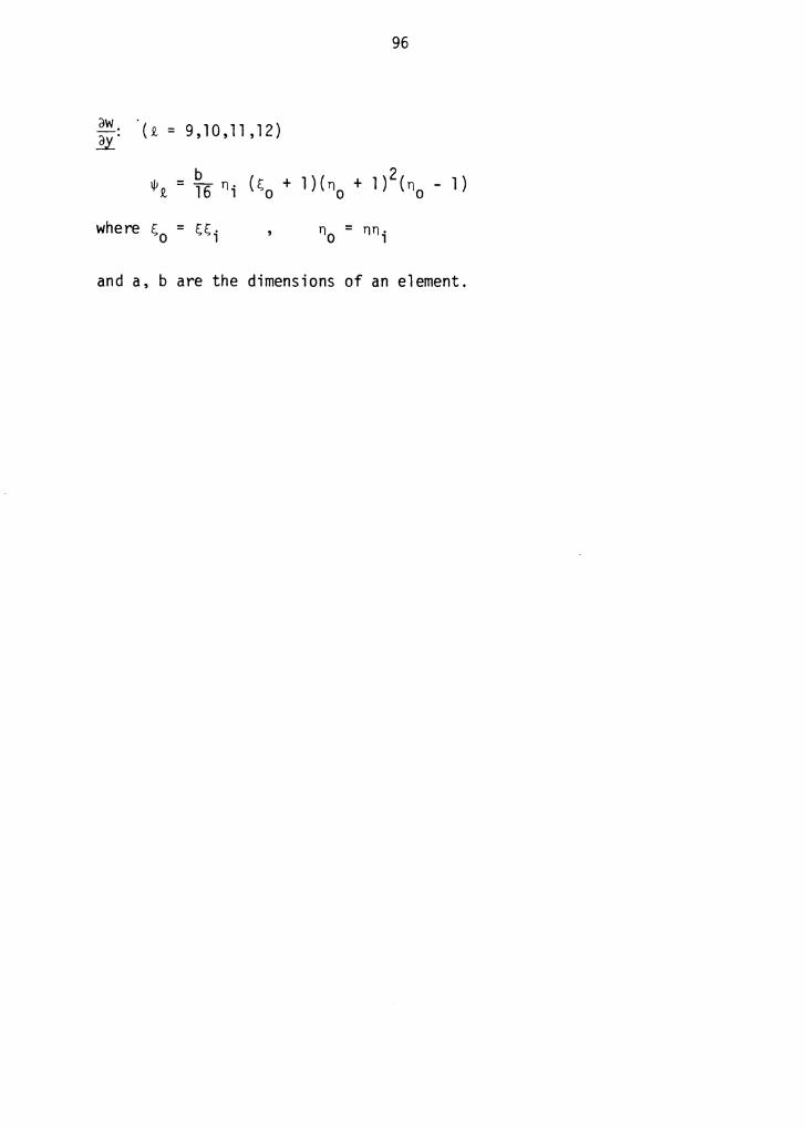
96

~: (t = 9,10,11,12)

"'i = ~6 n; (E;o + l)(no + 1)2(no - 1)

where E,;0 = E;E;i

and a, b are the dimensions of an element.

The vita has been removed from the scanned document