Nuclear Instruments and Methods in Physics Research A335 (1993) 276-287North-Holland

Linear and non-linear approaches to solve the inverse problem:applications to positron annihilation experiments

L. Hoffmann, A. Shukla, M . Peter, B . Barbiellini and A.A. ManuelUniversité de Genèse, Département de Physique de la Matière Condensée, 24, guai E. Ansermet, CH-1211 Genèse 4, Switzerland

Received 7 June 1993

We present linear and non-linear filters to solve the ill-posed inverse problem and we use them to extract relevant informationfrom positron lifetime and 2D-angular correlation of the annihilation radiation of positrons m solids . A general optimal linear filteris first derived Then a second linear approach, based on Bayes' theorem, is described. We show that these two linear approachesare indeed equivalent . Two non-linear methods are then discussed The first is a Bayesian approach which makes use of themaximum entropy principle . The second is an iterative method derived from the general optimal linear filter . Applications of thesefiltering techniques to positron lifetime decay curves illustrate how lifetimes shorter than the instrumental resolution can beextracted . Finally, we apply the iterative non-linear filter to the problem of the ridge-like Fermi surface on the high temperaturesuperconducting compound YBa 2Cu 307,. For the first time a direct measurement of the ridge width through a Brillouin zone isobtained . It is compared with results of band structure calculations .

1 . Introduction

1.1 . The inoerse problem

In this paper we are concerned with different ap-proaches for the resolution of the inverse problem,often encountered, in particular in experimentalphysics . The inverse problem occurs whenever dataavailable experimentally are to be used to determinedproperties of a physical phenomenon which are notdirectly accessible . The data are the known conse-quences of some unknown causes which we need todetermine. We write

fbK(x, y) 0(x) dx+N(y)=D(y) .a

This equation is an example of the Fredholm equationof the first kind . The problem is to determine theunknown function O(x) for a known kernel K(x, y)and known function D(y ), N(y) being a random func-tion with known standard deviation oy representingthe statistical noise. Let us illustrate this with someexamples which will be taken up later in the text . Eq .(1) could represent the convolution with an experimen-tal resolution function and addition of random noiseduring an experiment . In this case the kernel takes thesimple form K(x -y). The second example is that of apositron annihilation lifetime experiment in whichpositrons emitted by radioactive decay in a sourceannihilate in a crystalline sample . The time that elapsesbetween the emission of the positron and its annihila-tion by an electron can be measured and gives rise to a

decay curve when a large number of events arerecorded . This decay follows an exponential law with acharacteristic lifetime . In a given sample the positronmay annihilate with more than one lifetime and theinverse problem consists in determining these lifetimesfrom the measured decay curve. D(y) is the measureddecay curve; here y is the variable representing time .K(x, y) is the kernel of the equation which in the caseof the lifetime problem is given by x- i exp(-yx - 1 ), xbeing the variable which represents lifetime . O(x) isthe unknown intensity function which determines theintensity as a function of lifetime for a given experi-ment . For the third example we take the case of lineardata corresponding to a square function of unknownwidth buried in random noise. The kernel generates asquare feature of varying width and the unknown func-tion (P(x) picks out one (or more) widths with certainintensities to create the measured data .

1.2 . Solutions for the inverse problem

As we are concerned with discrete numerical solu-tions for eq . (1) we shall write it as a system of linearalgebraic equations where f represents the values ofF(x) at certain reference points,

Y_ k,w(bi<+n,=d,,il=ior matricially,

0168-9002/93/$06 .00 © 1993 - Elsevier Science Publishers B.V . All rights reserved

NUCLEARINSTRUMENTS& METHODSIN PHYSICSRESEARCH

Section A

K(P+N=D .

(2)

iP = K- 1D.

2. Theory

nd.,

L . Hoffmann et al. / Approaches

This is an "ill-posed problem" according to Tikhonov[1], one of the pioneers in the resolution of suchinverse problems . In the case of a physical experimentas opposed to the general case, the existence of asolution is usually guaranteed and in some cases eventhe uniqueness may be assured. K is usually not asquare matrix, because 0 and D need not have thesame dimension. However if we assume n mod = ndat wecan then, in principle, solve eq . (1) by inverting thematrix K,

This procedure leads in general to a meaningless resultbecause small errors in the process of inversion or inthe measurement of D lead to very large errors in (P .D(y) is not very sensitive to local variations in O(x)because the integration with the kernel smooths themout. However, small changes in D(y) can induce largevariations in O(x) as determined by the inversion of K[2,3] . The particular form of the kernel is also impor-tant for the stability of the system which is connectedto the eigenvalues of KK-1 [4]. The stability decreaseswith increase of the ratio between the largest andsmallest of the eigenvalues and this can be increasedsimply by augmenting the dimensions of the system,making any ill-posed problem potentially poorly deter-minate . This is the case for the earlier example of thepositron lifetime experiment .

Different methods have been used for the resolu-tion of the inverse problem and some have been re-viewed [3,5] . In the following paragraphs we will exam-ine linear and non-linear approaches to the problem.Two linear, one-step methods are used, based on theone hand, on the construction of a generalized optimalfilter inspired by the Wiener filter in image processing,and on the other hand on Bayes' theorem with aprobabilistic approach [3] and statistical regularization .These approaches are shown to be equivalent . Twonon-linear, iterative approaches are used, one usingthe principle of maximum entropy as the regularizingfactor [6,7], and the other based on the iterative applia-tion of the linear filter . These methods will then beapplied to extract information from measured and sim-ulated positron lifetime and 2D-angular correlation ofannihilation radiation (2D-ACAR) data, to show theirpossibilities and limits .

2.1 . Linear filters

The action of a linear filter can be written as

to solve the inverse problem

277

or matricially

where F is defined as the linear filter matrix of sizenmod - ndat . The problem is to find a suitable set ofcoefficients fW, to satisfy a certain criterion, generallyrealized by the extremization of a particular function .The linear filters described below act on the data D inthis manner . In non-linear approaches, the calculated4) depends non-linearly on the input D, (and 0,, if theapproach is iterative) .

2.2. General optimal linear filter

We design a linear filter F solving the inverseproblem (2) using the following procedure: we con-struct a filter matrix F given a criterion according towhich it should be optimal and using the knowledgeabout 0 and N. In the present case, F is designed tosatisfy a minimization criterion where the mean squareerror between the "real" 0 and the one extracted bythe filter from the data is minimized. One may alsominimize the mean square error between data andreconstruction directly but clearly one does not thensolve the inverse problem [8] . We write the minimiza-tion criterion as follows

Y_p�(I F(KO� +N) - (p � I Z )N minimum

The sum is over all linear combinations (each corre-sponding to a (P� and with an associated probability p� )of the nmod admissible models, averaged over all noiseconfigurations N contained in the data D . The expres-sion of the filter F is obtained after taking the deriva-tive of eq . (5) with respect to F, and setting it to zeroto satisfy the minimization criterion . The terms con-taining the first power of N are neglected since themean of the distribution of N is assumed to be zero .Solving eq. (5) leads to the expression of the generalfilter F, and the inverse problem is solved by theexpression of the regularized solution (PR:

,PR =FD,

where

F=C,pKT

KC,pKT +CN '

C,, and CN are the square autocorrelation matrices ofthe models and of the noise respectively . In the specialcases where the noise is uncorrelated, the mean overall possible noise configurations leads to a diagonalmatrix CN with o-,2 on the diagonal (or, is the standard

278

error in d) . It is interesting to note that C,1, is anidentity matrix when we are completely ignorant, thatis all possible combinations of the nmod different mod-els are admissible and equiprobable. In this case C~ isidentity for the same reasons as CN . Even if we restrictthe {0�} set to those 0, having a limited number ofnonzero elements (limiting the number of models M�present in D), C. is an identity matrix. We remarkthat using a {0�} set where v = 1 . . . n mod and each 0�corresponds to the presence of one of the nmod modelsforming the columns of the matrix K also leads to anidentity matrix for Cp, .

This filter (6) has a general character, in the sensethat other linear filters can be derived from it and isoptimal in the sense that it satisfies eq . (5) .

One of the special cases of the general filter is theclassical Wiener filter [1] . Its matrix elements are ofthe form f,, =f(i -j), where F - D is a convolutionproduct. For a square F matrix of size nddt ' nddt, eq .(5) can be simplified after a unitary transformation [8]in the Fourier space where F becomes diagonal andthe matrix operation F - D transforms to scalar filter-ing. The only information required for the constructionof the Wiener filter is the power spectra of 0� and N.The Wiener filter considers models which arc transla-tion invariant, and is therefore less selective than thegeneral filter .

Another special case is a scalar product, to whichthe general filter is reduced when K is an identitymatrix and for large constant noise with standard devi-ation Q . In this case the denominator of F is reducedto o- z and the filtered result is a projection of the dataD on the models.

The data transformation induced by the finite ex-perimental resolution function with which the experi-ment measures the models M can also be expressed asa special case of the general filter . In this case K - T isa simple convolution product. The rows of the kernelK contain the experimental resolution function, cen-tered on the diagonal of K.

2.3. Bayer' theorem

In analyzing data from physical experiments, proba-bilistic concepts come into play quite naturally, be-cause statistical error is random in nature and can becharacterized only in a probabilistic manner . Further-more, experimental data never have infinite resolutionand in particular in the case of ill-posed problems oneis forced to make inferences about various possibleresults or forms for the vector 0 given a certaindata-set D and an experiment described by the kernelK and the noise N. These inferences are best ex-pressed as conditional probabilities, p(O I D) . Lastly,as we have said before, the "ill-posed" nature of theproblem can be tackled by the process of regulariza-

L . Hoffmann et al. / Approaches to solve the inverse problem

tion . This regularization can be brought about by intro-ducing a priori information about the unknown quan-tity (P in the form of a "prior" probability distribution .These probability distributions will be linked togetherby Bayes' theorem to obtain meaningful informationabout P [3,7] .

The strategy is to make certain inferences about Pand calculate the associated probabilities. In otherwords, we wish to calculate the conditional probabilityp(0 I D) as a function of (P . This is not directly accessi-ble from the data which gives us the conditional proba-bility p(D I (P) often known as the "likelihood" . Thelikelihood depends on the characteristics of the mea-suring system and in the case where the probabilitydensity of the experimental noise is given by p�(N) wehave,

p(D I e) =p,,( D - KoP) .

(8)

For normally distributed noise this gives the distribu-tion

Il d,t

~~`p(D 1 oP) = II (217o-jZ)

=t

1

n-d

z

x cxp

-d J - Y_ kjw~wl

.2_ w-J

To jump from p(D I (P) to p(oP I D) we need the apriori probability density p(,P). This term also knownas the "prior" reflects the fact that we know only Dand helps us to decide on an estimate for (P, the "real"0 being unknown. We can now use Bayes' theorem toextract the a posteriori probability density p(oP I D) .Indeed we have

p( IP)p(D (P)p(oP I D) =

.

(10)

p(D)

p(D) is a constant normalizing factor . The a posterioriprobability depends on the experimental data as wellas the on the prior probability but of course maydepend much more on the one (which is generally thecase, when the data are "good") or on the other. Theusual strategy of smoothing data or minimizing theleast square error between data and reconstruction is aBayesian strategy with a constant, trivial prior. Theprior exerts a regularizing influence which makes itschoice an important step . The two methods discussedbelow use different approaches for the determinationof the prior probability .

2.4 . Linear Bayesian approach

The first approach (ref. [3] and references therein),is used in the event where one presumes known thecorrelation matrix C,,, (7) of the a priori ensemble . Thisis the identity matrix m the event when one knows

nothing. Out of the different sets of prior probabilities{p �} possible for the set of admissible vectors {(�]forming the a priori ensemble and leading to the givenC., we choose the set that minimizes the informationcontained in it about 0. This is the set {p �Πwhichmaximizes the expression :

and leads to a distribution density of the form [3]

p(p) a exp(-z(OTC-1,p ». (12)

For the purposes of this method only, the data and thekernel are transformed according to eq . (13) to takeinto account the fact that the standard deviations oferrors may be different for each component of thedata :

dJ = 0-Gm il,

and

k,', = GM kjb,,

(13)al

01

where o,,M is the geometric mean of the set {Q1} .However for reasons of simplicity we will continue touse the earlier notation (K and D instead of K' andD').

Using the expressions for p(D 14P) (10), p((P) (12)and Bayes' theorem we get p(0 I D), which is a Gauss-ian distribution . The regularized solution is given by

(PR = f0-p(OI D) d if) ,(14)

which amounts to maximizing p(~P I D) with respect togiving

COKT(PR C,pKTK+CND,

(15)

where for uncorrelated noise, CN= o'GM I, I being theidentity matrix of dimension nmod . With C, =I, eq .(15) simplifies to

2.5.2.5. Equivalence of the linear approaches

L. Hoffmann et al. / Approaches to solve the inverseproblem

(16)

The two linear approaches described in sections 2.2and 2.4 respectively, though motivated by differentconsiderations, give similar recipes (6) and (15) . In factthe filters found by the two methods are identical,which can be proved easily . For that we have to includethe transformation of D and K according to eq . (13),which may be written matricially as K'=XK andD'=_YD where 1 is a diagonal matrix with elementsa,MIo1 (we assume uncorrelated noise) . Let us assume

that both filtered data according to eqs. (6) and (15)are identical, which is expressed by

C,pKT(KC,,K T +CN) - 1 D

- (C pKTy2K+oGM I)-I C,KT_Y(_YD) . (17)

After cross-multiplication one obtains

C,KT_ 2 CN =o-c,C,,KT .

( 18)

Eq . (18) is satisfied, since CN may be written asaGM_y-2 . The optimal filter then, is equivalent to theone given by a Bayesian approach when the correlationmatrix C, for the given problem is known. Hencefor-ward we will not distinguish between the two andsimply refer to the linear filter .

It is worth noting that an identical expression to thelinear Bayesian filter described in eq. (16) (where C,, isidentity) is obtained [5] by minimizing the mean squaredeviation of the regularized solution KO R and thedata D in the measuring space under an a prioriconstraint as follows

ID-KORI2 +AIO R I2 minimum.

(19)

The constraint is the A-weighted term, regularizing thesolution in minimizing the square norm of vector 'PR.The parameter A quantifies the "smoothness" of thesolution . Considering K and D normalized accordingto eq . (13), we obtain easily the form of eq . (15), wherethe value of A is equal to o-GM .

2.6. Non-linear Bayesian approach : MaxEnt

In this approach [6,7] we seek solutions to theinverse problem in the form of positive additive densi-ties (PAD). It can be shown [71 that the prior probabil-ity distribution for a PAD is given by

Pr(O) a exp(aS(O, R)),

(20)

where S is the generalized Shannon-Jaynes entropy, Ran initial reference vector with respect to which theentropy is calculated (taken to be a constant [9]), and aa Lagrange multiplier (which is an inverse measure ofthe spread of the values of 1P about R) . S is given by

nm�d

S

ri

0', -ri,- 0~ log~

ru

.

279

(21)

Using Bayes' theorem once more, the a posterioriprobability distribution p(0 I D) becomes

Pr(e I D) a exp(aS - zX 2 ),

(22)

where we have used the definition

n-,,d 2

n d .,

( dj

kjAOwl

X 2 = Y

w=2

(23)j =1

0l

28 0

The solutions are found by maximizing the a posterioriprobability with respect to 0, which amounts to maxi-mizing the argument of the exponential term in eq .(22) . One may look for the most probable solution, orone corresponding to an adequate value for the X', ora set of solutions with the associated probabilities (theposterior "bubble") [7] . Various algorithms may beemployed, adapted to the specific nature of the prob-lem [10,11] .

We remark that in the formulation of the optimallinear filter, the regularized solution is found by ex-tremization (of the mean square error between the"real" solution and the regularized solution) with re-spect to the filter . In the Bayesian approaches theextremization (of the a posteriori probability) is withrespect to the regularized solution . This is similar tomechanisms where one can consider variations withrespect to the velocity (in the Lagrangian description)or to the momentum (in the Hamiltonian description) .

2.7. Non-!near iterative filter derived from the linearone- .step filter

The two Bayesian approaches differ in their expres-sions for prior probabilities . In the linear Bayesianapproach the information content of the prior proba-bility ensemble {p �] is minimized (or its "entropy"maximized) to arrive at the expression for p(O) . Max-Ent too maximizes an entropy as defined by eq . (21),where it is expressed using the components of T .However we must remember that the prior ensemblehere is restricted to PAD's so that the component (hwOf OR may be interpreted as the probability for thecorresponding model to be present, whereas in thelinear approach the regularized solution is not neces-sarily a PAD. This means that for problems where thesolution is effectively a PAD, some way will have to befound of eliminating any negative components in theregularized solution 'PR . Also, on the application ofthe linear, one-step filter on data where the solution isnot necessarily a PAD, we find that the regularizedsolution contains wide features and parasite oscilla-tions, for small signal to noise ratios . Here again onewould like to reinforce significant features in the solu-tion . We use iterative techniques where the solution isprogressively modified .We suppose that the prior ensemble {0w) is com-

posed of the nm~d solutions which each correspond tothe presence of one of the models included in thekernel matrix K with the associated prior probabilityensemble {p,) . On applying the filter to data, we canmodify the prior probability ensemble by diminishingthe probabilities p. of those models which are suppos-edly present with negative intensities, so as to intro-duce the PAD constraint . At each iteration we de-crease these p,, by a factor depending on the ratio of

L. Hoffmann et al. / Approaches to solve the incerse problem

negative intensities to positive intensities . The matrixC. remains diagonal but is no more equal to identity .This process can be iterated till the negative (~, com-ponents are eliminated . We remark that the PADconstraint may also be introduced solving eq . (19)iteratively [5] .

Another method of progressive modification of priorprobabilities was tried, and is also valid for the casewhere the PAD constraints does not exist . Here wesuppose that the amplitude 6. represents the ampli-tude of probability (AP) for the presence of the pthmodel such that the prior probabilities (pN ) for eachiteration are given by {d,2] where 0 is the outcome ofthe previous step . The process is continued till thesolution is stable, leading to the regularized solutionOR. This tends to reinforce the stronger features in thedata and suppress the features induced by noise.

We remark in both cases that the progressive modi-fication of prior probabilities has a sharpening effecton the significant features m (PR . The AP constraintcan separate closely spaced features more efficientlythan the PAD constraint but may on the other handsuppress significant features if they are present withsmall amplitudes . For small signal to noise ratios (ap-proaching unity), the iterative procedure does not im-prove the solution, as illustrated in a simulation de-scribed in section 3.3 .

3. Results and applications

3.1 Introduction

The following applications of the methods describedabove illustrate the resolution of the inverse problem,using simulated and measured data . The first applica-tion is the extraction of lifetimes and intensities frompositron lifetime spectra. This problem has alreadybeen investigated using the MaxEnt algorithm [12] .The second application is new. It is the characteriza-tion of a feature (a square function) within a 2D-ACARdistribution . Before starting with applications, it isworth remarking that experimental data often containa "background" or constant term which is not of inter-est and requires to be filtered out. This can be accom-plished in various ways . In the above formulations themodels M� forming the kernel K may be transformedso that their expectation value is zero . Alternatively, ifthe background can be measured independently, it maysimply be subtracted from the data D.

3.2 Positron lifetime

We present results obtained on applying the meth-ods discussed above for the resolution of the inverseproblem as encountered in analysis of positron lifetime

COUC

0.9

0.8

0.7

0.6

0.5

0.4

0.3

0.2

-0.10 50 100 150 200 250 300 350 400 450

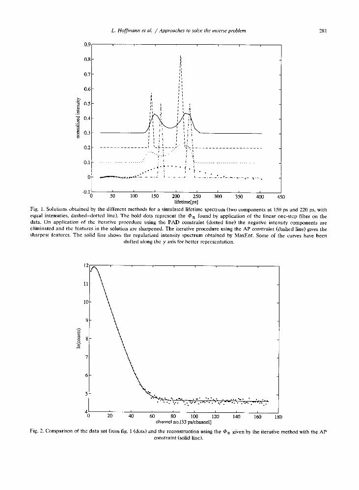
lifetime[ps]Fig. 1. Solutions obtained by the different methods for a simulated lifetime spectrum (two components at 150 ps and 220 ps, withequal intensities, dashed-dotted line). The bold dots represent the OR found by application of the linear one-step filter on thedata . On application of the iterative procedure using the PAD constraint (dotted line) the negative intensity components areeliminated and the features in the solution are sharpened. The iterative procedure using the AP constraint (dashed line) gives thesharpest features . The solid line shows the regularized intensity spectrum obtained by MaxEnt . Some of the curves have been

shifted along the y axis for better representation .

0

L. Hoffmann et al. / Approaches to solve the inverse problem

281

channel no.[33 ps/channel]

Fig. 2. Comparison of the data-set from fig. 1 (dots) and the reconstruction using the OR given by the iterative method with the APconstraint (solid line).

28 2

spectra. For all methods, we will use the same kernelmatrix K. The column vectors of this matrix are life-time decay curves corresponding to nmod = 115 differ-ent lifetimes sampled at ndat = 160 points (where thesampling interval is the same as for our experimentalsetup, that is 33 ps/channel) and convolved with theexperimental resolution function which is presumed tobe a Gaussian function of FWHM = 270 ps . The life-times increase exponentially from 20 ps to 6000 pswhich is sufficient to cover the range that we measure.Simulated data are convolved with the experimentalresolution function, contain Poisson noise and a con-stant background . Each simulated data-set is a lifetimespectrum with two components, at 150 and 220 ps andwith equal intensities . Ten data-sets were generatedwith the same characteristics and statistics (2 x 106counts), differing only due to the random noise con-tent .

Fig. 1 shows the solutions obtained by the differentmethods for one of the data-sets of the simulation . Thebold dots represent the OR found by application of thelinear one-step filter on the data . It can be seen thatthe solution is unsatisfactory in two respects . Firstlysome negative intensity components appear which weknow cannot exist as they do not correspond to aphysical process. Secondly, whereas the simulated data(dashed-dotted line) are generated by sharp peaks in

L. Hoffmann et al. / Approaches to solve the inverse problem

the intensity spectrum, the regularized solution con-tains smooth wide peaks centered on the sharp peaks.On application of the iterative procedure using thePAD constraint (dotted line) the negative intensitycomponents are eliminated and the features in thesolution are sharpened. The iterative procedure usingthe AP constraint (dashed line) gives the sharpestfeatures . Lastly we show the regularized intensity spec-trum (solid line) obtained by MaxEnt which is similarto that obtained with the PAD constraint iteration(details of application of the MaxEnt method to life-time spectra can be found in ref. [12]). Fig. 2 comparesthe data with the reconstruction using the OR given bythe iterative method with the AP constraint . Finallythe weighted residuals for the four methods are shown(fig . 3) . This illustrates the complexity introduced bythe inverse problem, as the reconstructions in themeasurement space are all very similar but the solu-tions in the intensity space are appreciably different . Intable 1 we summarize the results of the analysis on allthe ten data-sets by the MaxEnt method and the non-linear iterative method using the AP constraint. Bothapproaches give satisfactory results . The standard devi-ations of the lifetimes and intensities averaged over allthe data-sets are lower for the MaxEnt method. Thetwo components being equally intense though closelyspaced, the iterative method using the AP constraint

60 80 100 120channel no.[33 ps/channel]

140 160 180

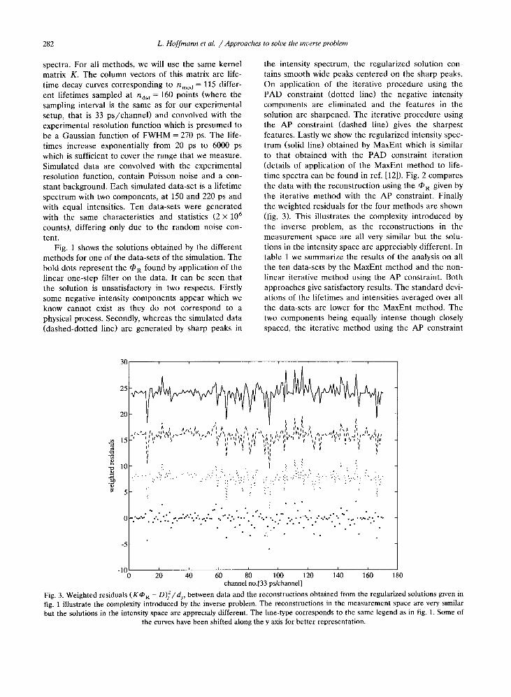
Fig. 3. Weighted residuals (KOR - D)'Idj

, between data and the reconstructions obtained from the regularized solutions given infig . 1 illustrate the complexity introduced by the inverse problem. The reconstructions in the measurement space are very similarbut the solutions in the intensity space are apprectaly different. The line-type corresponds to the same legend as in fig. 1 . Some of

the curves have been shifted along the y axis for better representation.

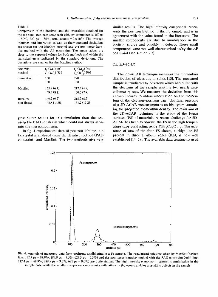
Table 1Comparison of the lifetimes and the intensities obtained forthe ten simulated data-sets (each with two components, 150 ps- 50%, 220 ps - 50%, total counts= 2 x 10 6 ). The averagelifetimes and intensities as well as their standard deviationsare shown for the MaxEnt method and the non-linear itera-tive method with the AP constraint . The mean values areclose to the expected values for both methods and within thestatistical error indicated by the standard deviations . Thedeviations are smaller for the MaxEnt method

gave better results for this simulation than the oneusing the PAD constraint which could not always sepa-rate the two components .

In fig . 4 experimental data of positron lifetime in aFe crystal is analyzed using the iterative method (PADconstraint) and MaxEnt . The two methods give very

0.25

0.2

0.15

0.05

L . Hoffmann et al. / Approaches to solve the inverse problem

100 200

Fe component

similar results . The high intensity component repre-sents the positron lifetime in the Fe sample and is inagreement with the value found in the literature . Thesmaller components are due to annihilation in thepositron source and possibly in defects. These smallcomponents were not well characterized using the APconstraint (see section 2.7) .

3.3. 2D-ACAR

The 2D-ACAR technique measures the momentumdistribution of electrons in solids [13] . The measuredsample is irradiated by positrons which annihilate withthe electrons of the sample emitting two nearly anti-collinear -y rays . We measure the deviation from thisanti-collinearity to obtain information on the momen-tum of the electron-positron pair . The final outcomeof a 2D-ACAR measurement is an histogram contain-ing the projected momentum density. The main aim ofthe 2D-ACAR technique is the study of the Fermisurfaces (FS) of materials. A recent challenge for 2D-ACAR has been to observe the FS in the high temper-ature superconducting oxide YBa2Cu 307 s . The exis-tence of one of the four FS sheets, a ridge-like FSpresent in three Brillouin zones (BZ), is now wellestablished [14-18]. The available data treatments used

source components

300 \ 400

Soolifetime[ps]

600 700 800

28 3

Fig. 4. Analysis of measured data from positrons annihilating in a Fe sample . The regularized solutions given by MaxEnt (dashedline : 112.7 ps - 89.8%, 284.8 ps - 9.5%, 629.5 ps - 0.5%) and the non-linear iterative method with the PAD constraint (solid line :112.4 ps - 89.9%, 288.5 ps - 9.5%, 681 ps - 0.6%) are quite similar. The high intensity component represents annihilation in the

sample bulk, while the smaller components represent annihilations in the source and/or crystalline defects in the sample .

Analysismethod

t, (At,) [Ps]11 (A1,) [%]

t2 (Ot 2 ) [Ps]12 (012 ) [%]

Simulation 150 22050 50

MaxEnt 153.9 (6 .1) 217.2 (4 .9)49 .4 (8 .1) 50 .6 (7 .9)

Iterative 149.7 (9 .7) 218.9 (8 .7)non-linear 48 .8 (13.0) 51 .2 (13.2)

284

in the positron annihilation community for observingthe FS are somewhat standard . However, in this com-pound, the FS induced structures are weak and thestatistical noise of the histogram becomes competitivein intensity. More sophisticated techniques are neededfor better characterization of this ridge-like FS inducedstructure.

We will assume that the shape and the center of theridge are known from theory, whereas we are inter-ested in measuring its width and intensity. The analysisof the intensity as a function of the ridge width is atypical application of the general linear filter describedin section 2.2, but is not well suitable to be solved bythe MaxEnt technique, since the result is not necessar-ily a PAD. First, different sections centered on theridge are extracted from the 2D-ACAR. Then a back-ground has to be subtracted from each section. Thisbackground is mainly induced by wavefunction modula-tions. For each section, the subtracted background is apolynomial of order 3 fitting the section in a least-squares sense, which conserves the ridge-like feature (athird order polynomial has only one inflection point) .These sections form a set of data D as described by eq .

côV

200

100

0

-100

L. Hoffmann et al. / Approaches to solve the muerse problem

(2). The n mod models M,, are defined as centeredsquare functions of equal intensity but of differentwidth characterized by ,tt . The kernel matrix K trans-forms the measuring space of the 2D-ACAR sectionsto the square function intensity space. Thus the lethcolumn of K contains the model M,, . The experimen-tal resolution function is taken into account by convolv-ing the models with this function . We also subtract thethird order polynomial fit from the models so that theyundergo the same treatment as the data D and lastlythe models are treated so that themean of the columnsof K is zero, rendering further filtering procedureindependent of constant background in the data D.For unknown correlations between the models, matrixC, is identity .

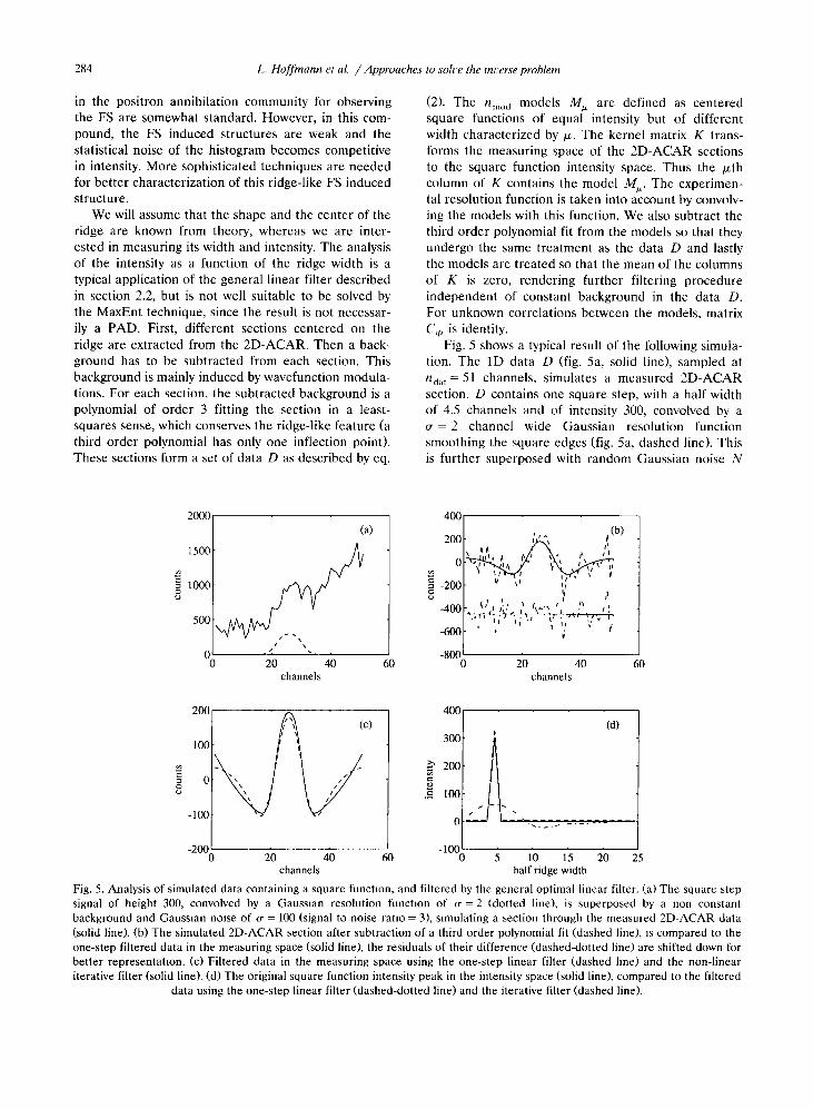
Fig. 5 shows a typical result of the following simula-tion . The 1D data D (fig . 5a, solid line), sampled at

ndac = 51 channels, simulates a measured 2D-ACARsection. D contains one square step, with a half widthof 4.5 channels and of intensity 300, convolved by ao, = 2 channel wide Gaussian resolution functionsmoothing the square edges (fig . 5a, dashed line). Thisis further superposed with random Gaussian noise N

400

200

0

0 -200U

-400

-600

-800

400

300

200c.S 100

0

0 20 40 60channels

-200

-1000 20 40 60

0 5 10 15 20 25channels

half ridge width

Fig. 5 . Analysis of simulated data containing a square function, and filtered by the general optimal linear filter . (a) The square stepsignal of height 300, convolved by a Gaussian resolution function of o, = 2 (dotted line), is superposed by a non constantbackground and Gaussian noise of Q = 100 (signal to noise ratio = 3), simulating a section through the measured 2D-ACAR data(solid line). (b) The simulated 2D-ACAR section after subtraction of a third order polynomial fit (dashed line), is compared to theone-step filtered data in the measuring space (solid line), the residuals of their difference (dashed-dotted line) are shifted down forbetter representation . (c) Filtered data in the measuring space using the one-step linear filter (dashed line) and the non-lineariterative filter (solid line). (d) The original square function intensity peak in the intensity space (solid line), compared to the filtered

data using the one-step linear filter (dashed-dotted line) and the iterative filter (dashed line).

of o, = 100 and a non-constant background . The squarefunction appears now to be drowned in the noise andthe background . The data D' (fig. 56, dashed line),obtained after having subtracted a polynomial fit ofdata D, is filtered by the one-step filter F described byeq . (6) with nmod = 25 square function models of vary-ing width. The reconstruction of the filtered data in themeasuring space is obtained by the operation KOR(fig . 5b, solid line). One observes that the noise isfiltered, leaving behind a smooth symmetric modula-tion (the symmetry is imposed by the symmetry of thesquare step models). The residuals KOR -D' (fig. 5b,dashed-dotted line, shifted for better presentation) arestructureless and thus reflect the noise. We applied theiterative procedure with the AP constraint, and thereconstruction thus obtained (fig . 5c, solid line) pre-sents a slightly different picture than the one-stepreconstruction (fig. 5c, dashed line). However the dif-ference in the intensity space is remarkable (fig. 5d),illustrating once again the precarious nature of theinverse problem. In fig . 5d, the abscissa represents thehalf width of the square functions . Both filtered datashow one correctly centered maximum. The one-step

20

L. Hoffmann et al. / Approaches to solue the inuerse problem

0 20 40x channels

L1\\\\\\\\\\\\M\\M

0 20 40x channels

filter (dashed-dotted line) produces a broad andsmooth distribution with some small negative compo-nents. The iterative procedure (dashed line) sharpensthe structure and makes the small components disap-pear, and OR now closely resembles the original inten-sity distribution (solid line).

In a general manner, for distributions made ofsharp peaks, the filtered data sharpened through thisiterative procedure are closer to the original distribu-tion than the one-step filtered data . However this istrue only above a given signal to noise ratio . To illus-trate this we analyzed a large number of data-sets for a51 channel distribution containing a 9.5 channel widesquare function convolved by a Gaussian resolutionfunction of o- = 1 channel. We found that the iterativemethod worked better with respect to the one-steplinear filter (in terms of mean square deviation be-tween O R and the "real" 0) for signal to noise ratiosgreater than 3. For smaller signal to noise ratios, noiseinduced structures amplified by the iterations becomeincreasingly dominant .

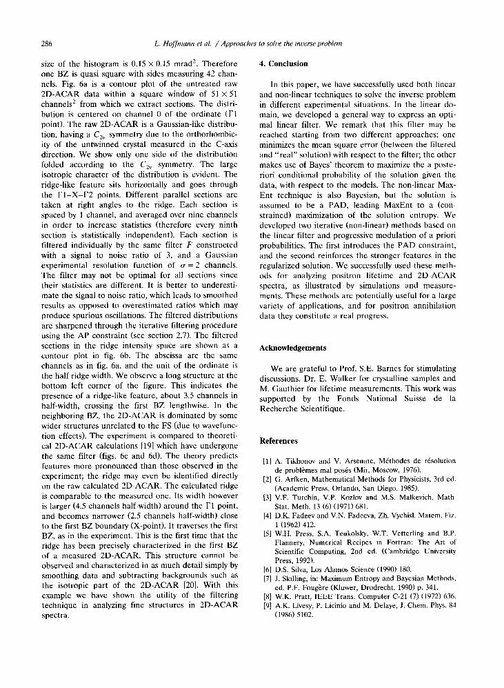
Fig. 6 shows the result obtained with a real 2D-ACAR measurement of YBa,Cu 3 0, s . The channel

0C-0o

a

0 20 40x channels

0 20 40x channels

285

Fig . 6 . Analysis of real 2D-ACAR results of YBa2Cu307 s using the iterative filter. (a) and (b) : Experiment ; (c) and (d) : FLÀPWcalculations . (a) and (c): Contour plot of the untreated raw 2D-ACAR data within a square window of 51 x 51 channels 2 . (b) and(d) : Contour plot of the iteratively filtered sections in the ridge intensity space. Signal to noise ratio = 3, Gaussian resolution

function width Q = 2 channels . Channel size = 0.15 mrad .

2010 b

0 3 150s

U01

010v10T

-105

-20U1006ORMMON,q1111j

20 (a)20

10ç 3 15

0 r

T -10 NEI ,r10

5-20

ii. MOM, �,��,

28 6

size of the histogram is 0.15 X 0.15 mrad2. Thereforeone BZ is quasi square with sides measuring 42 chan-nels. Fig. 6a is a contour plot of the untreated raw2D-ACAR data within a square window of 51 X 51channels 2 from which we extract sections . The distri-bution is centered on channel 0 of the ordinate (I'1point) . The raw 2D-ACAR is a Gaussian-like distribu-tion, having a C2,, symmetry due to the orthorhombic-ity of the untwinned crystal measured in the C-axisdirection. We show only one side of the distributionfolded according to the C2v symmetry . The largeisotropic character of the distribution is evident. Theridge-like feature sits horizontally and goes throughthe I1-X-I2 points . Different parallel sections aretaken at right angles to the ridge. Each section isspaced by 1 channel, and averaged over nine channelsin order to increase statistics (therefore every ninthsection is statistically independent). Each section isfiltered individually by the same filter F constructedwith a signal to noise ratio of 3, and a Gaussianexperimental resolution function of o, = 2 channels .The filter may not be optimal for all sections sincetheir statistics are different. It is better to underesti-mate the signal to noise ratio, which leads to smoothedresults as opposed to overestimated ratios which mayproduce spurious oscillations . The filtered distributionsare sharpened through the iterative filtering procedureusing the AP constraint (see section 2.7) . The filteredsections in the ridge intensity space are shown as acontour plot in fig . 6b . The abscissa are the samechannels as in fig. 6a, and the unit of the ordinate isthe half ridge width. We observe a long structure at thebottom left corner of the figure . This indicates thepresence of a ridge-like feature, about 3.5 channels inhalf-width, crossing the first BZ lengthwise . In theneighboring BZ, the 2D-ACAR is dominated by somewider structures unrelated to the FS (due to wavefunc-tion effects). The experiment is compared to theoreti-cal 2D-ACAR calculations [19] which have undergonethe same filter (figs . 6c and 6d). The theory predictsfeatures more pronounced than those observed in theexperiment ; the ridge may even be identified directlyon the raw calculated 2D-ACAR. The calculated ridgeis comparable to the measured one. Its width howeveris larger (4 .5 channels half-width) around the 171 point,and becomes narrower (2 .5 channels half-width) closeto the first BZ boundary (X-point). It traverses the firstBZ, as in the experiment . This is the first time that theridge has been precisely characterized in the first BZof a measured 2D-ACAR. This structure cannot beobserved and characterized in as much detail simply bysmoothing data and subtracting backgrounds such asthe isotropic part of the 2D-ACAR [20] . With thisexample we have shown the utility of the filteringtechnique in analyzing fine structures in 2D-ACARspectra.

L. Hoffmann et al. / Approaches to solve the inverse problem

4. Conclusion

In this paper, we have successfully used both linearand non-linear techniques to solve the inverse problemin different experimental situations. In the linear do-main, we developed a general way to express an opti-mal linear filter . We remark that this filter may bereached starting from two different approaches ; oneminimizes the mean square error (between the filteredand "real" solution) with respect to the filter ; the othermakes use of Bayes' theorem to maximize the a poste-riori conditional probability of the solution given thedata, with respect to the models . The non-linear Max-Ent technique is also Bayesian, but the solution isassumed to be a PAD, leading MaxEnt to a (con-strained) maximization of the solution entropy. Wedeveloped two iterative (non-linear) methods based onthe linear filter and progressive modulation of a prioriprobabilities. The first introduces the PAD constraint,and the second reinforces the stronger features in theregularized solution . We successfully used these meth-ods for analyzing positron lifetime and 2D-ACARspectra, as illustrated by simulations and measure-ments. These methods are potentially useful for a largevariety of applications, and for positron annihilationdata they constitute a real progress .

Acknowledgements

We are grateful to Prof. S.E . Barnes for stimulatingdiscussions, Dr. E. Walker for crystalline samples andM. Gauthier for lifetime measurements . This work wassupported by the Fonds National Suisse de laRecherche Scientifique .

References

[1] A. Tikhonov and V. Arsenure, Méthodes de résolutionde problèmes mal posés (Mir, Moscow, 1976).

[2] G. Artken, Mathematical Methods for Physicists, 3rd ed .(Academic Press, Orlando, San Diego, 1985).

[3] V.F . Turchin, V.P . Kozlov and M.S . Malkevich, MathStat. Meth . 13 (6) (1971) 681.

[4] D.K. Fadeev andV.N . Fadeeva, Zh . Vychisl . Matem. Fiz .1 (1962) 412.W.H . Press, S.A . Teukolsky, W.T . Vetterling and B.P .Flannery, Numerical Recipes in Fortran : The Art ofScientific Computing, 2nd ed . (Cambridge UniversityPress, 1992).

[6] D.S . Silva, Los Alamos Science (1990) 180.[7] J . Skilling, in : Maximum Entropy and Bayesian Methods,

ed . P.F . Fougère (Kluwer, Drodrecht, 1990) p. 341.W.K . Pratt, IEEE Trans. Computer C-21 (7) (1972) 636.A.K. Livesy, P. Licinio and M. Delaye, J. Chem . Phys. 84(1986) 5102 .

[81[91

[10] R.K. Bryan, in : Maximum Entropy and Bayesian Meth-ods, ed . P.F . Fougère (Kluwer, Dordrecht, 1990) p. 221.

[11] J. Skilling and R.K . Bryan, Mon. Not. R. Astr . Soc. 21 1(1984) 111 .

[12] A. Shukla, M. Peter and L. Hoffmann, this issue, Nucl .Instr . and Meth . A335 (1993) 310.

[13] S. Berko, in: Momentum Distributions, eds. R.N . Silverand P.E . Sokol (Plenum, 1989).

[14] L.C. Smedskjaer, A. Bansil, U. Welp, Y. Fang and K.G.Bailay, J. Phys . Chem . Solids 52 (1991) 1541 .

[15] H. Haghighi, J.H . Kaiser, S. Rayner, R.N . West, J.Z. Liu,R. Shelton, R.H . Howell, F. Solal, P.A. Sterne and M.J .Fluss, J. Phys. Chem . Solids 52 (1991) 1535 and Phys .Rev. Lett . 67 (1991) 38 .

L. Hoffmann et al. / Approaches to solve the inverse problem 287

[16] M. Peter, A.A . Manuel, L. Hoffmann and W. Sadowski,Europhys . Lett . 18 (1992) 313.

[17] A.A . Manuel, B. Barbiellini, M. Gauthier, L. Hoffmann,T. Jarlborg, S. Massidda, M. Peter, W. Sadowski, A.Shukla and E. Walker, J. Phys . Chem . Solids, to bepublished .

[18] B. Barbiellini, M. Gauthier, L. Hoffmann, T. Jarlborg,A.A . Manuel, S. Massidda, M. Peter, W. Sadowski, A.Shukla and E. Walker, Physica C 209 (1993) 75 .

[19] S. Massidda, Physica C 169 (1990) 137.[20] M. Peter, T. Jarlborg, A.A . Manuel, B. Barbiellini and

S.E . Barnes, Z. Naturforsch . A48 (1993) 390.