linear and radial flow modelling of a waterflooded

Journal Pre-proof

Linear and radial flow modelling of a waterflooded, stratified, non-communicatingreservoir developed with downhole, flow control completions

Bona Prakasa, Khafiz Muradov, David Davies

PII: S0920-4105(19)30761-2

DOI: https://doi.org/10.1016/j.petrol.2019.106340

Reference: PETROL 106340

To appear in: Journal of Petroleum Science and Engineering

Received Date: 26 May 2019

Revised Date: 1 August 2019

Accepted Date: 3 August 2019

Please cite this article as: Prakasa, B., Muradov, K., Davies, D., Linear and radial flow modellingof a waterflooded, stratified, non-communicating reservoir developed with downhole, flow controlcompletions, Journal of Petroleum Science and Engineering (2019), doi: https://doi.org/10.1016/j.petrol.2019.106340.

This is a PDF file of an article that has undergone enhancements after acceptance, such as the additionof a cover page and metadata, and formatting for readability, but it is not yet the definitive version ofrecord. This version will undergo additional copyediting, typesetting and review before it is publishedin its final form, but we are providing this version to give early visibility of the article. Please note that,during the production process, errors may be discovered which could affect the content, and all legaldisclaimers that apply to the journal pertain.

© 2019 Published by Elsevier B.V.

https://doi.org/10.1016/j.petrol.2019.106340



Linear and radial flow modelling of a waterflooded, stratified, non-communicating

reservoir developed with downhole, flow control completions

Summary

Forecasts of the performance of waterflooded oil-field have been prepared for many years

using fractional flow models, such as those by (Buckley-Leverett, 1942) (BL), (Welge, 1952)

and (Dykstra-Parsons, 1950) (DP), to estimate the vertical sweep efficiency between wells.

These methods, and their later modifications, formed the theoretical basis for designing a

water-flooded oil-field. Advanced Well Completions (AWC) incorporating downhole flow

control device (FCD) technology have become a proven method for modifying a production

well’s inflow profile, delaying water breakthrough, improving sweep efficiency and enhancing

recovery.

This manuscript extends the fractional flow model describing the performance of a

waterflooded, stratified-reservoir with an AWC installed in the production well. The piston-like

behaviour of the water-front described by previous, semi-analytical models is extended here

to the linear and radial flow modelling of more realistic displacement profiles.

This paper describes the theoretical basis and application workflow along with several

case studies illustrating their performance and value. The accuracy of the new, semi-analytical

models are verified by comparison against the results from a numerical reservoir simulator.

Model limitations and possible future extension are also discussed.

The workflow can be implemented as either a production forecast or a diagnostic tool for

an AWC well in a waterflooded oil-field. It provides one missing link between today’s AWC

design workflows and the long-term value evaluation of a specific AWC design when a

commercial numerical simulation software is either not available or too time consuming.

1. Introduction

Researchers have developed simplified performance and analysis methods based on

(semi-) analytical solutions and type curves for a range of well control situations, well patterns

and geological environments in a waterflooded oil-field. These simplified analysis methods are

still routinely used today, despite the wide availability of numerical reservoir simulators.

The oil recovery factor is the product of the oil efficiency displacement at the pore

level and the volumetric sweep efficiency. The latter, a product of the areal and vertical sweep

efficiencies, is a function of the flood pattern, geological discontinuities, mobility ratio, etc. The

vertical sweep efficiency between an injection and production well pair depends on the

reservoir heterogeneity with more permeable layers being flooded faster.

(Buckley and Leverett, 1942) provided the first description of two-phase, immiscible

displacement of oil by water in a linear (1D) pore system. Their BL model described the velocity

water propagation through the linear system. (Welge, 1952)’s W model calculates the average

saturation behind the water front, establishing a relationship between the average water

saturation as a function of either the cumulative volume of water injected or the total injection

time. They are recognised as proven methods for forecasting oil recovery with conventional

wells, but are not applicable to production wells completed with DFC, a technology designed

to mitigate unevenly propagating waterflood fronts in heterogeneous reservoirs.

The areal sweep and oil displacement efficiencies has been widely studied, e.g. the

(Dyes et al., 1954) mathematical model or core flooding experiments. This paper presents a

new method to predict and analyse the vertical sweep efficiency of an oil field developed with

AWC production wells. Analytical solutions for the vertical sweep efficiency of a

heterogeneous reservoir refer to either non-communicating or to perfectly communicating

layers with instantaneous pressure equilibrium.

The (Dykstra and Parsons, 1950) (DP) model analysed the case of non-communicating

layers case with arbitrary properties. Their analytical solutions estimate the recovery efficiency

and the fractional flow curve of each layer as a function of the volume of injected water. They

also derived general formulae and type curves for a reservoir with a vertical, log-normal,

permeability distribution. (Muscat, 1950) derived expressions for other permeability

distributions while (Johnson, 1956) extended the solutions to cases where the water-oil

viscosity ratio is no longer one. (Synder and Ramey, 1967) used elements of BL theory to add

non-piston-like displacement, note that non-piston like displacement occurs when the mobility

ratio is significantly higher or lower than one. (Osman and Tiab, 1981) extended the model to

composite layers with lateral permeability variation while (Reznik et al., 1984) and (El-Khatib,

1985) translated the results into the time domain.

(Warren, 1964) and (Goddin et al., 1966) considered the effect of crossflow between

layers. Solutions for waterflood analysis in reservoirs with communicating layers were

presented by (Hiatt, 1958) and extended to reservoirs with layers of variable properties (El-

Khatib, 1985), log-normally distributed vertical permeability (El-Khatib, 1999), gravity driven

cross-flow (El-Khatib, 2003) and even inclined reservoirs (El-Khatib, 2010). Finally, (Muradov, et

al., 2018) extended the DP model to AWC wells for stratified-reservoir waterfloods with piston-

like oil-water displacement behaviour typical of fluids with a mobility ratio close to unity. Their

solution included the non-linear, pressure versus flow rate performance of FCDs.

Waterflood performance with radial flow was analysed by (Muscat, 1950) while (Deppe,

1961) predicted the changing injection rates in radial flow for cases with unequal fluid mobility

and irregular well patterns. (Rossen, et al., 2008) extend fractional-flow methods for two-

phase flow to non-Newtonian fluids in one-dimensional cylindrical flow, where rheology

changes with radial position, r, thus allow the fractional-flow curve as a function of radial

position. Wu, et al., 2010, presented analytical solutions for non-Darcy flow linear and radial

composite reservoir based on Forchheimer and Barree-Conway solution. Mijic, A., and T. C.

LaForce (2012) presented the extension of the Buckley-Leverett analytical solution in radial

flow when the injected gas phase flow is governed by the two-phase extension to the

Forchheimer equation and the fractional flow function depends both on the saturation and

radial distance from the well. Evaluation of a peripheral waterflood was presented by (Ling,

2016) using a fractional flow approach to solve for radial flow. This paper shows how fractional

flow analysis can be applied to predicting the performance of an AWC well.

The (Halliburton, 2017), steady-state wellbore simulator is the most frequently used tool

to predict the performance of an AWC well. This workflow provides a good estimate of the

AWC well’s performance for the well and near-wellbore reservoir parameters at a specific

time. However, (Livescu et al., 2010) recognised that the preferred AWC design for early-time

production parameters may no longer be optimum once the long-term well’s performance

(cumulative oil and water, sweep efficiency, etc.) are considered.

This paper develops a simple, practical workflow to evaluate the long-term performance of

an AWC well without the need for numerical, reservoir simulation software. The novel aspects

of this work are the extension of the:

1. Welge method with a more accurate relative permeability value of the formation

behind a displacement he front at a given average water saturation.

2. Analytical, Buckley-Leverett fractional-flow analysis workflow of non-piston like

displacement of reservoir fluids flowing towards an AWC well. Solutions for both linear

and radial flow are provided.

3. Model to quantify the change in the FCD’s restriction as a function of the water cut.

2. Review of fractional flow analysis and the extended P method to include AWCs

AWC wells are employed when producing from zones of differing reservoir quality,

such as heterogeneous reservoirs, differentially depleted layers, compartmentalized

reservoirs, multiple-reservoir developments, unfavourably saturated (e.g. oil-rim) reservoirs,

etc. Passive FCD also reduce a long completion’s “heel-to-toe effect”(Birchenko et al.,

2010a,b). AWC can be installed in a horizontal, deviated or multi-lateral well. An AWC well has

between one and hundreds of FCDs installed in the production tubing opposite the production

interval.

Figure 1: Schematic view of a well with an AWC.

Figure 1 is a schematic view of an open-hole AWC installed with three packers

providing annular flow isolation. Optimum AWC design is a complex mathematical problem

requiring specification of the FCD type, restriction level and the number of devices. The

performance of these FCDs can be represented with the help of a simple empirical constant,

called the segment’s FCD strength (a), and the segment flow rate (Q). ∆�� = �� (1)

where a, the ‘strength’ parameter relates the extra pressure drop, ∆�, added by the

fluid flow rate, Q. (Al-Khelaiwi, 2013) provides formulae to quantify the ‘strength’ parameter.

The pressure drop across the FCD’s restriction is a non-linear function of the fluid flow

rate (equation 1), unlike the linear dependence of the reservoir pressure drop. A greater

pressure drop occurs across those FCDs with a higher inflow rate. The result is a more uniform

inflow profile along the length of the completion compared with that expected from a

conventional (open-hole or perforated) completion. FCDs may be Passive (a fixed restriction),

Active (a surface controlled restriction) or autonomous (the restriction increases when

producing an unwanted fluid). (Eltaher et al. 2014, Al- Khelaiwi et al. 2008) a good overview of

the various types of FCD technology, their evolution and their applications.

i. Passive FCD designs are all essentially a fixed restriction that obeys equation 1.

ii. Active FCDs typically have between 2 and 10 positions, each of which has a different

‘strength’ value described by equation 1 { see (Haghighat Sefat et al. 2016}.

iii. Autonomous FCDs restrict the flow (Eltaher et al. 2014) in the presence of an unwanted

fluid phase (free gas and/or water). The ‘strength’ parameter is now a function of the type

of (single-phase) fluid and the phase-cut (Eltaher et al., 2018; Muradov et al., 2018).

The industry’s standard, FCD snapshot design uses a stand-alone wellbore simulator

coupled to near-wellbore reservoir simulation {e.g. (Halliburton, 2017)}. The wellbore model

optimises the “added-value” by altering the AWC performance specifications to reduce the

flow imbalance between zones while avoiding too great a restriction to the inflow

performance. This fast, simplified approach improves the initial (oil) production and is

assumed to increase the oil long recovery. This assumption is normally not rigorously tested by

reservoir simulation.

Alternative, snapshot models exist. (Birchenko et al., 2010) developed analytical and

semi-analytical methods to reduce the “heel-toe effect” in homogeneous and heterogeneous

(Birchenko et al., 2011) reservoirs. (Al-Khelaiwi 2013) proposed numerical workflow based on a

wellbore model as well as an inflow-outflow balance method. (Prakasa et al, 2015, Prakasa et

al, 2019) employed a type-curve method for FCD completion design.

Snapshot methods lack the ability to predict the AWC’s long-term impact on the oil

recovery efficiency of the waterflood. Traditionally, prediction of the long-term, reservoir

performance requires use of a complex, time intensive, coupled wellbore-reservoir simulator.

This paper offers an alternative to this problem.

2.1. Fractional flow analysis (linear immiscible displacement)

The BL model describes two-phase, immiscible displacement in a linear system. Equation

2, the fractional flow equation, leads to equation 3 which calculates the location � � of a given

water saturation (��, with following assumptions: capillary pressure effects can be neglected,

no dip, thus gravity forces can be neglected, homogeneous and isotropic porous medium.

�� = �� !��"��"�� (2)

� �#� = $%�&' ()"(*"+#" (3)

�� is fractional flow or the ratio of the flow of water at any point, A is cross-section area, , is

permeability, ,-. and ,-� is relative permeability of oil and water respectively, /$ is total rate, 0. and 0� is viscosity of oil and water respectively, �1 is capillary pressure, t is time, Φ is

porosity, �� is water saturation.

(Welge, 1952) evaluated the average saturation behind the water front by drawing a

tangent to the ��curve originating at the initial water saturation ��3� (Figure 2). Point A, the

intersection, is �� at the flood front and the reciprocal of the slope is the water front’s

velocity. The average saturations behind this front is found by extrapolating the tangent �� = 1.

Figure 2: An example of fractional flow curves analysis

(Welge, 1952) determined the average water saturation at breakthrough ��5$666666�, point

B in figure 2, by integrating the water saturation over the distance from the point of injection

to value of the saturation at the flood front. The calculation continues post-breakthrough

(equation 4) with the tangent line to �� = 1 being drawn to find the average water saturation

The calculation stops once the layer is fully saturated with water, i.e. when (�� = 1 7 �8-). ��9:; = ��6666 = ��< = >�?<�@A"@B" C (4)

2.2. Fractional flow analysis (radial immiscible displacement)

Figure 3: Flow in a circular reservoir with a well at the cenre: left – vertical view, right – lateral view.

The BL method for linear immiscible displacement was modified for radial flow by

(Ling, 2016) and verified by (Zhang, 2013). Radial fractional flow is described by equation (5)

while equation (6) calculates the position of a specified water saturation. These underlying

assumptions of equation 2 and 3 were also applied for equation 5 and 6, that were: capillary

pressure effects can be neglected, no dip and gravity forces can be neglected, homogeneous

and isotropic porous medium. They enable the fractional flow evaluation of the water front

position, the breakthrough time and oil recovery performance for a radial waterflooded oil

reservoir.

�� = ��DEF�� -�� G�!��"��"�� (5)

H#� = HI 7JHI 7 K�LMN �O<"O#"!#" (6)

HI is radius of the reservoir outer boundary, H#�is the position of water saturation Sw in the

radial system, WI is the cumulative volume of injected water, h is the reservoir thickness in the

radial system (see Figure 3 ).

2.3. Review of DP method and its extension to incorporate AWC performance

An injection and a production well are a distance L apart in a heterogeneous reservoir

with non-communicating layers being waterflooded with piston-like displacement (Figure 4).

Figure 4: Oil displacement between an injection well and a production well in a heterogeneous reservoir.

Each layer has unique properties: height h, effective cross-sectional area A, porosity φ,

horizontal permeability k, end point saturations Swi and Sor. All fluid volumes and Darcy velocity

(Uo and Uw) are measured at reservoir conditions.

Mobility of displacing phase: λ�̀ ≡ V�"`W" (7)

Mobility of displaced phase: λ.̀ ≡ V��`W� (8)

End-point mobility ratio X ≡ Y"̀Y�̀ (9)

Z. = 7 [Y\̀∆G�]?^ (10)

Z� = 7 [Y"̀∆G"^ (11)

Where L is the distance between injector and producer, and x is the waterfront’s distance to

the injector, Figure 5 shows layer j when the waterfront has travelled to coordinate xj.

Figure 5: Saturation profile in Layer j.

All fluids are assumed to be incompressible, hence Uo=Uw=U. Also, ∆P=∆Po+∆Pw allowing

equation 10 and 11 to be combined to give the oil production rate (equation 12).

/_ = _̀a_ = [bY",b` &b] ∆Gcb∗�eb��?cb∗! (12)

Where x* is defined as dimensionless front distance x_̀ ≡ ^b]

(Dykstra and Parsons, 1950) provided a workflow for estimating the vertical sweep efficiency

of a heterogeneous oil reservoir with non-communicating layers and piston-like fluid

displacement. They provide an analytical solution for the water front position x in arbitrary

Layer j at the exact time when the given reference Layer R is experiencing water breakthrough

(i.e. when x*R=1 so Layer R is flooded). The integral solution can be expressed explicitly as:

_∗ = eb?JebD�gb,hi�?ebj��eh�eb?� (13)

Where k_,l ≡ [bY",b`∆#b∅b . ∆#h∅h[hY",h` and.

The movable fluid saturation, ∆S, defined as ∆S =1-Swi-Sor, allows equation 13 to be simplified

to _∗ = gb,h��eh� when Mj=1.

The distance of the waterfront, and the water volume injected, in a layer after it has

been flooded may be found by changing the integration limits. The water front location in the

remaining layers can be calculated at the time when the first, or reference, layer experiences

breakthrough. The overall reservoir saturation, the injected water volumes and the production

well’s fractional flow fw (or watercut WC) can all be calculated at this time. The reservoir water

saturation and the injected water volume as a function of the production well’s WC is

calculated by repeating the workflow as the next, and each subsequent, layer experiences

water breakthrough.

(Reznik et al., 1984) and (El-Khatib, 1985) accurately included time into the model by

integrating the analytical solution for xj . We will show later that time can be approximated by

matching the injection rates and the injected volumes, i.e. *

,

1R

Rbt R

R at x

WIt

q =

≈ for AWCs by

including the reservoir-to-AWC well, pressure drop system (Figure 6).

Figure 6: Calculation of fluid saturation profiles in layer j when FCDs are installed.

The pressure drop across the sandface flow control completion (∆PFCC) is a quadratic

function of the flow rate where a is a function of the FCD strength, the number of FCDs per

completion zone and the flowing fluid’s properties (Al-Khelaiwi, 2013):

∆�g�� = �<o.�3p;qM9rI/ (14)

∆Po,j ∆Pw,j

∆P = P injector well – P producer well

∆Pfcd

xj L - xj

So = Sor,j Sw = Swi,j

Wa

ter

fro

nt

FCD length is negligible

For simplicity we refer to �<o.�3p;qM9rI as aw and ao for water and oil flow respectively. The

total pressure drop across a layer is now a function of both the reservoir and the FCD:

∆� = ∆�3p_I1$.- =∆�o9sI- = ∆�q-.tu1I- = i�3p_ = �q-.tj/ = ∆�o9sI- = �∗/ = ∆�o9sI-

(15)

where *a for a given layer equals

* *, ,bbt w inj o proda a a a≡ = + before water breaks through this

layer, and * *

, ,abt w inj w proda a a a≡ = + after water breakthrough. Changing the a coefficients

allows modelling of any type of FCD for any or all layers:

• A Passive FCD, an Active FCD or an Autonomous FCD completion: The a coefficients are

selected to match the number and type of FCD’s for each layer for either oil (producer

before break through) or water (injector and producer after break through).

• a = 0 for a conventional well (no FCDs).

• aw,prod =∞ or qabt=0 represents closure of the zone by a well workover, an Active FCD or

an Autonomous FCD responding to a change in the flowing fluid’s phase cut.

Rearranging equation (15) calculates the layer sandface-to-sandface pressure drop

(∆Player):

∆�o9sI- = ∆� 7�∗/ (16)

Substituting ∆P for ∆Player in equation (12) results in

' * 2,

* *(1 )j w j j j j

jj j j

k A P a qq

L x M x

λ ∆ −= ⋅

+ − which is

input into the equation u=q/A to yield:

Z_ = ?vb�JvbD�w9b∗&bD�bD∆G9b∗&bD�b (17)

where coefficients B and C are defined as:

x_ ≡ _∗ =X_i1 7 _∗j (18)

y_ ≡ [b�Y",b`] (19)

N.B. The original DP method includes the effective layer cross-sectional area when

calculating the flow rates and watercuts. Our study of AWCs case requires the area to be

introduced immediately since it affects the reservoir pressure drop. The effective cross-sectional

area must be estimated, taking into account e.g. the areal sweep efficiency, flood patterns,

faults, etc. (Muradov, et al., 2018) provides the complete derivation, verification and

application of the DP method extended to AWCs for the piston-like fluid displacement.

3. Extending waterflood analysis with AWCs to non-piston-like displacement

3.1. Application of the Welge method for calculation of oil and water production rates

Figure 7: The formation volume behind the flood front is divided into multiple blocks

Welge analysis was developed to determine the oil recovery and the water fraction as

a function of cumulative volume of water injected for non-piston-like displacement. The Welge

method calculates the formation’s water saturation (S{6666) behind the flood front assuming the

oil is homogeneously displaced with water. The formation behind this flood front has a

“pseudo” relative-permeability, |-�66666&|-.66666, based on the average water saturation, S{6666, (Ahmed, 2001); (Craig, 1993) and (Dake, 2001) all proposed predicting the front’s displacement

by finding the Kr values by direct correlation from the value of S{6666 based on the actual relative-

permeability curve. This assumes both piston-like displacement and linear relative-

permeability curves.

Figure 7 illustrates waterflooding a layer’s formation volume between the producer

and the injector. ��refers to pressure at the injection well’s location ( ~) or at the start time of

the displacement process. �<is the pressure at <, the tip of saturation front where water is

displacing oil. The difference between pressure �� and �< is ∆��. Mobile oil is present in the

formation between the water front and the producer (� 7 <). ∆�� is the pressure difference

between the displacement front and the production well’s annulus and ∆�g��.-g�� is the

pressure different across the FCDs. Figure 7 indicates that FCDs are only installed in the

producer, an extra pressure drop, ∆�g��3, must be added to ∆�� if FCDs are also installed in

the injection well.

P1 Sw1

Krw1, Kro1

∆P1

Sw1

Krw1, Kro1

∆P1

Swn

Krwn, Kron

∆Pn

SwN

KrwN, KroN

∆PN

Pf

∆n1 ∆nn ∆nN

Figure 8: Several blocks with different relative permeability values are created behind the water front.

1 - Sor

∆n3

Sw3

Sw average

∆n1

Sw1

∆nN

Swf

∆nn

Swn

∆n2

Sw2

Swc

0

0.1

0.2

0.3

0.4

0.5

0.6

0.7

0.8

0.9

1

Sw

xn1 x2 x3 x4x0

P1

P1P

f

∆Pw ∆Po ∆PFCC

P2 P

ann

Krw & Kro are unique for each block due to

differences in saturation and permeability

xf L - x

f

Length of FCC

is negligible

Swf

~ <

The water saturation value (Sw) of the formation between the injector and the water

front gradually decreases from (1 – Sor) at the injector to Swf at waterfront (Figure 7). This can

be modelled by a series of blocks with appropriate water saturation and relative permeability

values (Figure 8) starting from ~ to �� (= ∆�� and continuing to block N and ∆�� (or <�. �� 7 �<�, the pressure difference between ~ and <, is equal to the sum of the pressure

drops across all the blocks between ~ and < (Figure 8 and equation 20).

�� 7 �< = ∑ ∆�p�p�� (20)

As displayed in figure 8, the region between ~ and < is consisted with unique Krw & Kro for

each blocks. Our proposed method treated this region as a one block with an averaged relative

permeability value for each phase, Krwavg and Kroavg. Thus, neglecti

ng capillary pressure:

Z� W"�A[[-�� = �Z� W"�^�?^\�[[-�� = Z� W"�^D?^��[[-�D =⋯! = Z� W"[ �∑ ∆^�[-��p�� !

The average oil and water relative permeability behind the water front are:

,H�9:; = �A∑ ∆ ��"�� = �A∑ ∆ B"��"B"B"A��B�� (21)

,H89:; = �A∑ ∆ �� = �A∑ ∆ B��B"B"A��B�� (22)

The mobility value of the displacing phase behind the flood front together with the system

mobility ratio (equation 23 and 24) is now calculated:

��3^,t3rqo913p;qM9rI = [6�"�" = [6�� (23)

X8��8 = X = e��e�� = ¡� ,��F�� (24)

The BL method determines both the position, p, and its saturation value, ��p. (Dake,

2001) explains that the position of any water saturation is proportional to the derivative of

fractional flow over the water saturation (equation 25), allowing the position of each

saturation block relative to the front (equation 26) to be determined.

¢#� ∝ O<"O#"+#� (25)

�B"��B"A ∝ �A"�B"+B"��A"�B"+B"A (26)

This approach will be called the ‘Extended Welge’ (EW) method.

3.2. Extension of linear fractional flow analysis to include AWCs.

Fractional flow analysis integrating the extended DP, BL and EW methods, as per

(Muradov, 2018)’s methodology, is possible by adding the FCD’s, non-linear pressure drop to

the system (equation 15). The fluid velocity in each layer is:

Z_ = ?vb�JvbD�w9b∗&bD�bD∆G9b∗&bD�b (27)

Where coefficients B and C are:

x_ ≡ _∗ =X_i1 7 _∗j (28)

y_ ≡ [b ¡� ,��F��] (29)

Note that one of the main difference with the extended DP method’s equation is the

value of the mobility ratio of the displacing phase, �9:;,t3qo913p;qM9rI, as explained in

following section.

3.2.1 Workflow for extending linear fractional flow analysis to include AWCs.

Time period between the start of injection and water breakthrough in layer R

Step 1. Fractional flow analysis is carried out using relative permeability values to

calculate, and draw, the �� and ��¤ curves, find the value for the flood front saturation and the

average water saturation (Figure 2: , equation 4 and 5). The saturation front (��<) and average

water saturation��̅) behind the front are constant prior to breakthrough. |H89:; and |H�9:; of the displacing front will also be constant during this period.

Step 2. The evaluation is for every incremental x starting from the ~ (the location of

injector) to L (the location of producer). E.g. An injection and a production well are 1000 m

apart and evaluated at 10 m intervals, thus ~ represents the injection wells location, ∆ = 10m, L = 1000m, and hence �~~ is the producer’s location. Note that this ∆x grid is

different to the N blocks in Figure 8 that represented the multiphase fluid properties. Strictly

speaking, there are N blocks each time the front advances by Δx with the incremental

cumulative water injection �∆¨©[� being evaluated using equation 30 (i.e. fractional flow

analysis is executed for every xn).

∆¨©^ = Gªt<" t#"« + ∗ ∆ (30)

Averaging the injection rate between Ic?�andIc gives the incremental time (equation 31):

∆�^ = ∆K� � ,9:; (31)

Equation 24 calculates the mixed fluids’ mobility ratio, the injection rate is given by equations

17, 18, 19 and the total injection time by equation 32:

�^ = ∑ ∆�^�̂�� (32)

Step 3. The above is repeated for each layer of the well’s completion. Layer R, the

reference layer, is the first layer to experience breakthrough and the remaining layers are

ordered by increasing breakthrough time. The time required for the water to advance by Δx in

layer R (equation 33) is also used to calculate the distance �∆ _,^) the water advances in the

other layers (layer J). This distance is approximated by replacing the right side of equation 33

with equations 30 and 31.

∆�l,^ = ∆�_,^ (33)

∆�l,^ = Gª°t<" t#"« +b ∗ ∆^b, �b, ,9:; (34)

The first two parameters± ²³´µ)¶ µ*¶« +·¸on the right-hand side of equation 34 are constant

before breakthrough at ��_, hence only Δx needs be calculated. The injection rate (I) is also a

function of Δx, a simple non-linear solver (e.g. Excel, Matlab) can determine this in a fraction of

second.

Step 4. Repeat step 3 until layer R experiences breakthrough. Flow-in and flow-out of

the system are equal (i.e. �. = ©) during this time period. No water is produced and �� = 0.

Time period after initial water breakthrough until all completion layers are producing water.

Step 5. The second layer to experience breakthrough is now designated as layer R and

steps 3 and 4 are repeated until water breaks through into all remaining layers. The post-water

breakthrough into those layers experiencing water breakthrough (layer K) is calculated by

evaluating every incremental �� starting from the initial flood front saturation, ��[, until

when oil production stops, i.e. �� = �1 7 ��l�. E.g., layer K experiences an initial water front

saturation of 0.45 and has a residual oil saturation of 0.2. The oil and water production rates

are calculated by equation 35, 36 and ©¹ = ��. = ��¹. This is repeated in increments of ∆�� = 0.05from ��[,� = 0.45 to ��[,¼ = 0.80, after which Layer K produces 100% water.

�. = �<" 7 © (35)

�� = © 7 �. (36)

Equations 37 provides the time required to increase ∆��by0.05 in layer R. This time is also

used to calculate the increase in water saturation in the other layers (layer K).

∆�l,^ = ∆�[,r (37)

Layer K’s increase in the water saturation (∆�[,r) is approximated by replacing the right hand

side of equation 37 with equations 30 and 31.

∆�l,^ = �t<" t#"« +�,�∗��,�,�� ∗ �Àl (38)

Water has already broken through in layer K. Hence, equation 38 it is now necessary to

determine the first two parameters on the right-hand-side of equation 38, �µ)¶ µ*¶« +ÁiÂÃ,Á,ÄÅÆj,

both of which are function of Sw. A non-linear solver is required to solve for the value for ��[,r

also provides the change in the mixed fluid’s mobility ratio (equation 29) and the injection rate

(equations 17, 18 and 19).

Step 5a. An extra calculation step is required to evaluate the (variable) “strength”

parameter (a*abt) when autonomous FCDs are installed This is obtained from equation 39

(Halvorsen, Elseth and Nævdal, 2012; Mathiesen, Werswick and Aakre, 2014).

��95$∗ = ÇÈ�K�∗É"�∗i��?K��∗É�jÊDÉ�� Ë ∙ Ç ��È�K�∗�"�∗i��?K��∗��jÊËs ∙ �&�� (39)

Steps 5 and 5a are repeated until all layers are producing water.

Time period after all layers have experienced water breakthrough.

Step 6. All layers are designated layer k apart from layer R, the last layer to

experience breakthrough. The step 5 workflow continues is repeated until the well’s oil

production ceases and �� = �1 7 ��l� in all layers (equation 40).

∆�l,^ = ∆�[,r

�t<" t#"« +h,�∗�h,�,�� ∗ �Àl = �t<" t#"« +�,�i��,�,��j ∗ �À[ (40)

Step 7. Summing each layer’s performance: cumulative oil produced, Íq (equation

41), cumulative water produced, q̈ (equation 42), cumulative water injected, 3̈p_ (equation

43) at any time.

Íq = ∑ �.3o|$ ∙ ∆�p$�~ (41)

q̈ = ∑ ��9$I-|$ ∙ ∆�p$�~ (42)

3̈p_ = ∑ �3p_Ï$ ∙ ∆�p$�~ (43)

3.2.2. Extending the workflow for constant well production

The workflow for constant rate well production requires approximating the layer rates

prior to the breakthrough at an arbitrary pressure drop by calculating the flow rates at every x

(equations 27, 28 and 29). Their sum gives the total well rate. The pressure drop required for

the chosen well rate is found as previously with an optimisation routine. This process is

repeated for each Δx prior to breakthrough after which it is repeated for each ΔSw increment.

3.3. Radial fractional flow analysis extended to an AWC.

The total layer pressure drop from the reservoir boundary to the well (equations 44

and 45) is the sum of the pressure drops across the: (1) displacing phase from the external

reservoir radius, re, to the flood front, rf, (2) displaced phase from the flood front, rf, to the

wellbore radius, rw, and (3) flow through the flow control completion:

∆� = ∆��3rqo913p; = ∆��3rqo91It = ∆�g�� (44)

∆� = %op>��ACM[ ¡� = %op��A�"!M[ � = �∗/ (45)

Rearranging equation 45 gives:

�_ = ?vb�JvbD�w9b∗iG�?G"Aj9b∗ (46)

Where:

x_ ≡ �Ðop>��AC�op��A�"!M[ � (47)

The section 3.1. workflow for linear displacement is followed to obtain ��3^ by

discretising the displacing phase into N blocks to find the average oil and water relative

permeability values for radial flow (equations 48 and 49):

,H�9:; = op> ��AC∑ Ñ��>�� C��"� Ò��

(48)

,H89:; = op> ��AC∑ Ñ��>�� C�� Ò��

(49)

The water front’s advance in radial displacement is no longer directly proportional to

the derivative of fractional flow. The radial case requires the position (��p�) for each saturation

block (��p) to be solved with equation 50, a modified version of equation 6. Fractional flow

analysis assumes incompressible fluids and volume replacement, hence the cumulative water

injected �¨©� equals the cumulative liquid produced �À�. Àp = Gªt<" t#"« +� ∗ ∑ ∆�ppp��

� = HI 7JHI 7 ª�LMN �O<"O#"!#"� (50)

AWC cases with radial flow replace the Δx employed for linear displacement with Δr.

4. Verification of the waterflood, analytical model.

4.1. A single layer, linear waterflood

A single layer, box, reservoir model with a cross sectional area of 30 m2 and 500 m

spacing between the production and the injection wells was constructed in the ECLIPSETM

numerical reservoir simulator for validation of our analytical, waterflood performance

workflow. The 50 bar pressure difference between the two wells and the oil/water mobility

ratio of 5 ensured linear, non-pistonlike, oil displacement. Table 1 summarises the other

reservoir properties. The production well’s autonomous FCD completion had a pre-

breakthrough strength (�55$∗ ) of 0.008 bar/(rcm/d)2 which gradually increased to 0.064

bar/(rcm/d)2 at 100% WC.

Table 1 - Well adata for the linear flow, waterflood validation test

Parameters K W h ϕ Swi Sor kwe koe μw μo no nw ÓÔÔÕ∗ ÓÓÔÕ∗ ∆P

Units mD m m cP cP ��H�HÖ×/Ù��

bar

Value 4000 10 3 0.4 0.2 0.15 0.5 0.95 0.4 4 2 3 0.008 0.064 50

,-. = ,-.I � �#�?#��?#"�?#��!p� (51)

,-� = ,-�I � �#"?#"��?#"�?#��!p" (52)

(Brooks-Corey, 1966)’s relative permeability curves (equations 51 and 52) allow explicit

calculation of the �� and ��¤ values (equations 53 and 54). no and nw, are the Brooks-Corey

exponents for oil and water and kroe and krwe are the relative permeability curve end points.

�� = �±��"�� ∙��"�∙�B��B��∙��B"��B��"�B"�B"��"��B"��B�� ¸ (53)

��¤ = t<"t#" = �� 7 �� p��?#"?#��= p"�#"?#"��! (54)

Figure 9 finds the water saturation at the flood front (��< = 0.575), and the average

saturation behind the front (��9:; = 0.65). The calculation is repeated at 50 m intervals

between injector’s ( ~) the producer’s ( �~) location. The discretised harmonic average (HA)

method with 50 blocks behind the front, (i.e. N=50), for calculating the average relative-

permeability (equations 21 and 22) and estimating �3p_ and �. for each block better

reproduced the ECLIPSETM results than the Welge method (Figure 10 and Table 2). This

mismatch increased further after water breakthrough (Figure 10).

Table 2: Comparison of the average relative permeability prior to water breakthrough

Figure 9: Numerical and analytical comparison of

fractional flow analysis for a linear waterflood

Figure 10: The harmonic average and Welge

methods compared

Our analytical model’s water and oil production rates agree well with the results of

numerical simulation (Figures 11 and 12).

0

0.2

0.4

0.6

0.8

1

0.0 0.2 0.4

fw

fwdfw/dsw

0.0

0.2

0.4

0.5 0.6 0.7

Re

lati

ve P

erm

ea

bili

ty

Sw

Average relative permeability

after breakthrough

Kro-avg Welge Krw-avg Welge

Kro-avg HA Krw-avg HA

Average relative permeability prior to

water breakthrough

Kro-avg Krw- avg

Harmonic Average 0.01 0.15

Welge 0.13 0.13

Figure 11: Water and Oil production rates

Figure 12: Water Injection (WI) versus water-cut (fw)

4.2. A single layer, radial waterflood

The reservoir radius (re) is 91.4 m, the thickness (h) 1.52 m and the permeability is 0.2

Darcy. The production well, 0.03 m diameter, is completed with autonomous FCDs of strength

(�55$∗ ) 0.011 bar/(rcm/d)2 prior to breakthrough, increasing gradually to 0.043 bar/(rcm/d)2 at

100% WC. Voidage replacement and a constant ΔP was maintained between the wells. Fluid

properties are as per section 4.1. Table 3 summarises the well and reservoir data.

Table 3 - Well and reservoir data for the radial flow, waterflood validation test.

The linear-flood workflow was followed with the average permeability being

calculated by the Welge and HA methods. The same fluids properties were used, giving the

same saturation values at the flood front and the average saturation behind the front (��< =

0.57 and ��9:; = 0.65). However, the HA relative permeability values in radial flow are

different (Figures 13 and 14) since they are calculated at positions (Xj) that depend on a

logarithmic calculation of the front’s position.

Figure 13: Average relative permeability calculation

methods before breakthrough for a radial flood

Figure 14: Average relative permeability calculation

methods after breakthrough

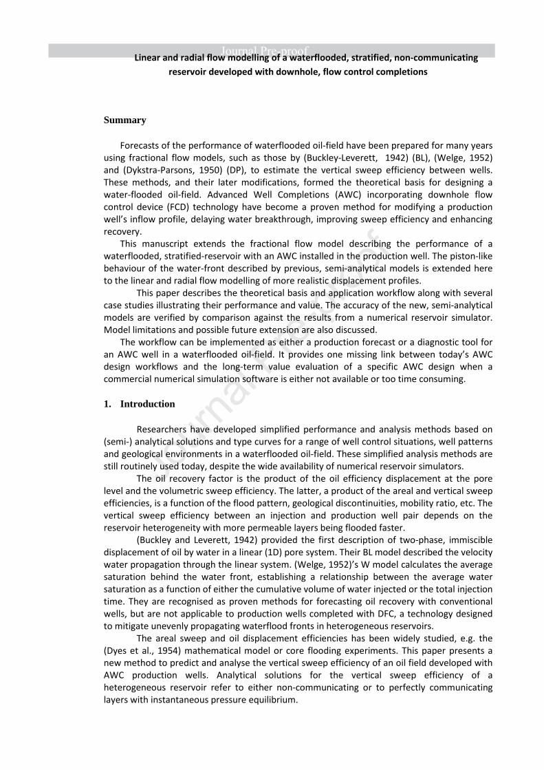
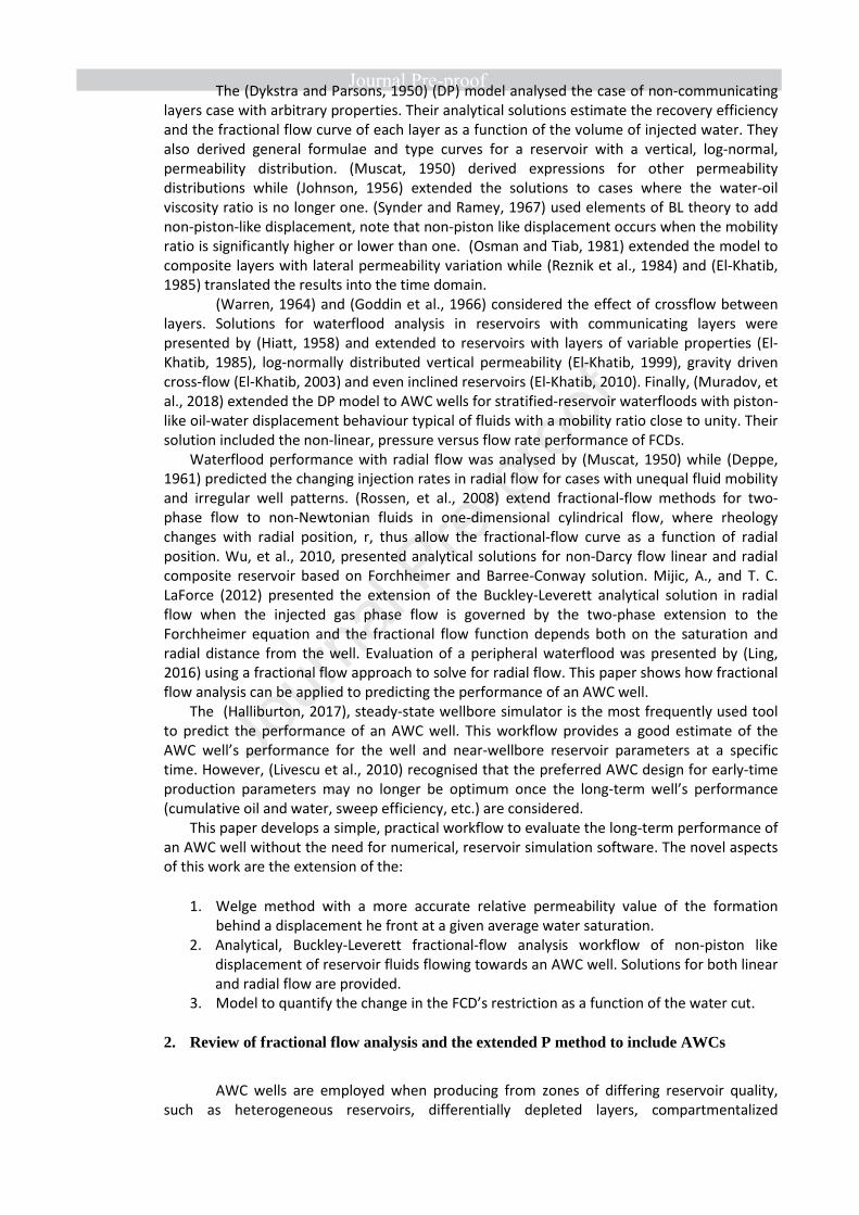
The fluid production rates before and after breakthrough (Figure 15) and the fractional flow

evaluation (Figure 16) validate our analytical methods against the EclipseTM reservoir

simulator.

0

50

0 200 400

Sm3/D

ay

Days

Oil Rate - Numerical ResultsWater Rate - Numerical ResultsOil Rate - Proposed MethodWater Rate - Proposed Method

0

0.5

1

0 2 4

fw

WI

Numerical Results

Analytical Results

0.0

0.1

0.2

0.0 0.2 0.4 0.6 0.8 1.0

Re

lati

ve P

erm

ea

bili

tie

s V

alu

es

Blocks, Xj

Kro-avg HA Krw-avg WelgeKrw-avg HA Kro-avg Welge

0.0

0.1

0.2

0.3

0.4

0.5

0.5 0.6 0.7 0.8 0.9

Re

lati

ve P

erm

ea

bili

tie

s V

alu

es

Water Saturation, SwKro-avg HA Krw-avg Welge Krw-avg HA Kro-avg Welge

Parameter K re rw h ϕ Swi Sor kwe koe μw μo no nw ÓÔÔÕ∗ ÓÓÔÕ∗ ∆P

Units Darcy m m m cP cP bar/(rcm/d)2 bar

Value 0.2 91.4 0.03 1.52 0.2 0.2 0.10 0.5 0.95 0.4 4 2 3 0.011 0.043 289

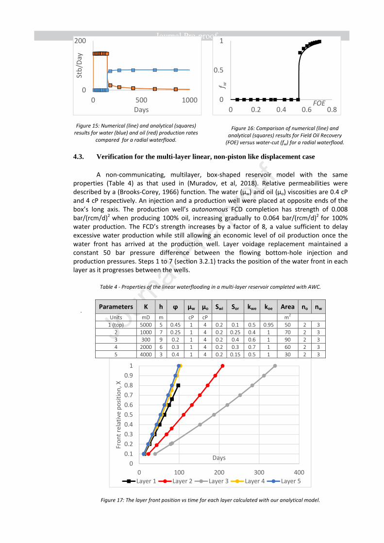
Figure 15: Numerical (line) and analytical (squares)

results for water (blue) and oil (red) production rates

compared for a radial waterflood.

Figure 16: Comparison of numerical (line) and

analytical (squares) results for Field Oil Recovery

(FOE) versus water-cut (fw) for a radial waterflood.

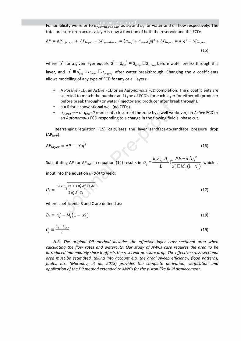
4.3. Verification for the multi-layer linear, non-piston like displacement case

A non-communicating, multilayer, box-shaped reservoir model with the same

properties (Table 4) as that used in (Muradov, et al, 2018). Relative permeabilities were

described by a (Brooks-Corey, 1966) function. The water (μw) and oil (μo) viscosities are 0.4 cP

and 4 cP respectively. An injection and a production well were placed at opposite ends of the

box’s long axis. The production well’s autonomous FCD completion has strength of 0.008

bar/(rcm/d)2 when producing 100% oil, increasing gradually to 0.064 bar/(rcm/d)2 for 100%

water production. The FCD’s strength increases by a factor of 8, a value sufficient to delay

excessive water production while still allowing an economic level of oil production once the

water front has arrived at the production well. Layer voidage replacement maintained a

constant 50 bar pressure difference between the flowing bottom-hole injection and

production pressures. Steps 1 to 7 (section 3.2.1) tracks the position of the water front in each

layer as it progresses between the wells.

Table 4 - Properties of the linear waterflooding in a multi-layer reservoir completed with AWC.

.

Figure 17: The layer front position vs time for each layer calculated with our analytical model.

0

200

0 500 1000

Stb

/Day

Days

0

0.5

1

0 0.2 0.4 0.6 0.8

f w

FOE

0

0.1

0.2

0.3

0.4

0.5

0.6

0.7

0.8

0.9

1

0 100 200 300 400

Fro

nt

rela

tive

po

siti

on

, X

Days

Layer 1 Layer 2 Layer 3 Layer 4 Layer 5

Parameters K h ϕ μw μo Swi Sor kwe koe Area no nw

Units mD m cP cP m2

1 (top) 5000 5 0.45 1 4 0.2 0.1 0.5 0.95 50 2 3

2 1000 7 0.25 1 4 0.2 0.25 0.4 1 70 2 3

3 300 9 0.2 1 4 0.2 0.4 0.6 1 90 2 3

4 2000 6 0.3 1 4 0.2 0.3 0.7 1 60 2 3

5 4000 3 0.4 1 4 0.2 0.15 0.5 1 30 2 3

Figure 18 and Figure 19 are snapshots of the numerically simulated, water saturation

at xR = 0.4 and xR = 0.8 for the bottom, highest permeability, reference layer where the initial

water breakthrough occurs. The improved sweep efficiency of the autonomous FCD

completion compared to screen completion is illustrated in Figures 20 and 21, water saturation

snapshots for the screen completion at the same time step as Figures 18 and 19.

Figure 18: Layer water saturation at XR = 0.4 for the

autonomous FCD completion

Figure 19: Layer water saturation at XR = 0.8 for the

autonomous FCD completion

Figure 20: Layer water saturation profile for the

screen completion at the time step as Figure 18.

Figure 21: Layer water saturation profile for the

screen completion at the time step as Figure 19.

The workflow calculates a different value of the injection rate Qinj for each Xn in order

to maintain voidage replacement along with the position of the water front in the time domain

(Figure 22). The average, layer Krw, Kro values change such that the injection rate in layer 5

increases during the first 100 days prior to break after which its flow is restricted by the FCD.

The process is repeated as each subsequent layer experiences breakthrough, resulting in the

layer flow rates being relatively more equal as the flood continues.

Figure 22: Predicted layer flow rates over time

0

10

20

30

40

50

60

0 100 200 300 400 500

Sm3/d

ay

Days

Layer 3Layer 1Layer 2Layer 4Layer 5

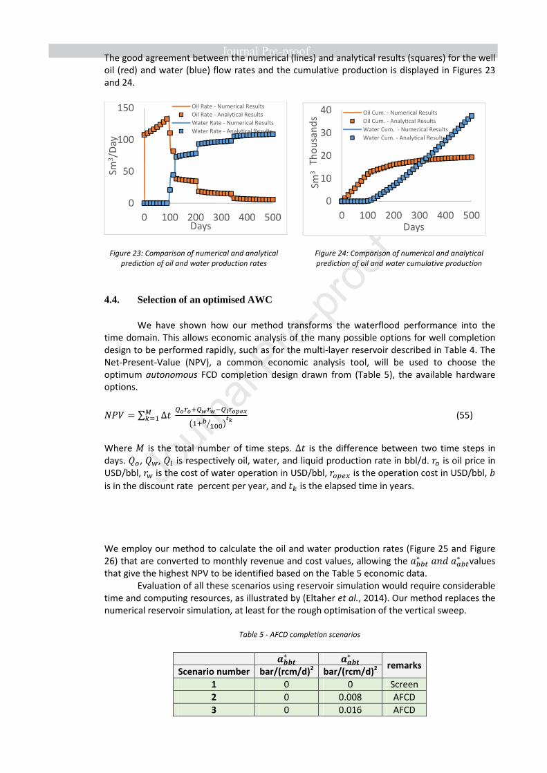
The good agreement between the numerical (lines) and analytical results (squares) for the well

oil (red) and water (blue) flow rates and the cumulative production is displayed in Figures 23

and 24.

Figure 23: Comparison of numerical and analytical

prediction of oil and water production rates Figure 24: Comparison of numerical and analytical

prediction of oil and water cumulative production

4.4. Selection of an optimised AWC

We have shown how our method transforms the waterflood performance into the

time domain. This allows economic analysis of the many possible options for well completion

design to be performed rapidly, such as for the multi-layer reservoir described in Table 4. The

Net-Present-Value (NPV), a common economic analysis tool, will be used to choose the

optimum autonomous FCD completion design drawn from (Table 5), the available hardware

options.

Í�À = ∑ ∆� Ú�-��Ú"-"?Ú�-�� i��5 �~~« j��e[�� (55)

Where X is the total number of time steps. ∆� is the difference between two time steps in

days. �., ��, �o is respectively oil, water, and liquid production rate in bbl/d. H. is oil price in

USD/bbl, H� is the cost of water operation in USD/bbl, H.qI^ is the operation cost in USD/bbl, �

is in the discount rate percent per year, and �[ is the elapsed time in years.

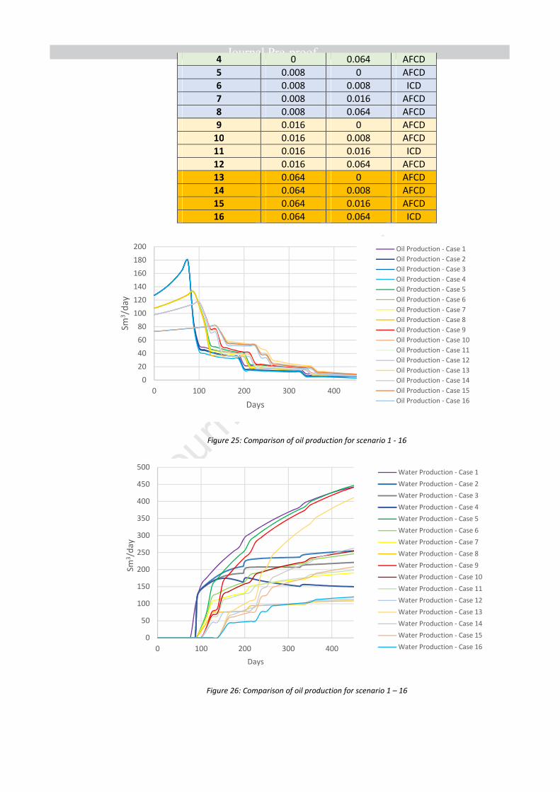
We employ our method to calculate the oil and water production rates (Figure 25 and Figure

26) that are converted to monthly revenue and cost values, allowing the �55$∗ ��Ù�95$∗ values

that give the highest NPV to be identified based on the Table 5 economic data.

Evaluation of all these scenarios using reservoir simulation would require considerable

time and computing resources, as illustrated by (Eltaher et al., 2014). Our method replaces the

numerical reservoir simulation, at least for the rough optimisation of the vertical sweep.

Table 5 - AFCD completion scenarios

ÓÔÔÕ∗ ÓÓÔÕ∗

remarks Scenario number bar/(rcm/d)2 bar/(rcm/d)2

1 0 0 Screen

2 0 0.008 AFCD

3 0 0.016 AFCD

0

50

100

150

0 100 200 300 400 500

Sm3/D

ay

Days

Oil Rate - Numerical Results

Oil Rate - Analytical Results

Water Rate - Numerical Results

Water Rate - Analytical Results

0

10

20

30

40

0 100 200 300 400 500

Sm3

Th

ou

san

ds

Days

Oil Cum. - Numerical Results

Oil Cum. - Analytical Results

Water Cum. - Numerical Results

Water Cum. - Analytical Results

4 0 0.064 AFCD

5 0.008 0 AFCD

6 0.008 0.008 ICD

7 0.008 0.016 AFCD

8 0.008 0.064 AFCD

9 0.016 0 AFCD

10 0.016 0.008 AFCD

11 0.016 0.016 ICD

12 0.016 0.064 AFCD

13 0.064 0 AFCD

14 0.064 0.008 AFCD

15 0.064 0.016 AFCD

16 0.064 0.064 ICD

Figure 25: Comparison of oil production for scenario 1 - 16

Figure 26: Comparison of oil production for scenario 1 – 16

0

20

40

60

80

100

120

140

160

180

200

0 100 200 300 400

Sm3/d

ay

Days

Oil Production - Case 1
















0

50

100

150

200

250

300

350

400

450

500

0 100 200 300 400

Sm3/d

ay

Days

Water Production - Case 1
















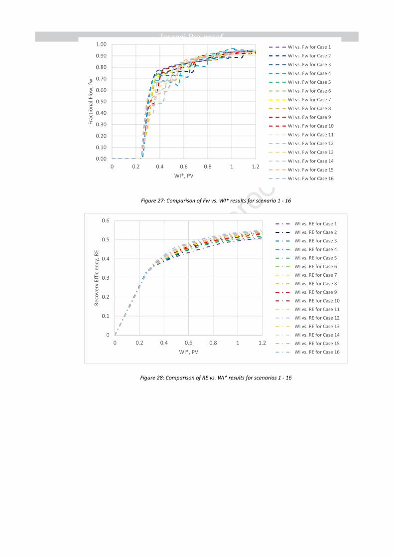
Figure 27: Comparison of Fw vs. WI* results for scenario 1 - 16

Figure 28: Comparison of RE vs. WI* results for scenarios 1 - 16

0.00

0.10

0.20

0.30

0.40

0.50

0.60

0.70

0.80

0.90

1.00

0 0.2 0.4 0.6 0.8 1 1.2

Fra

ctio

na

l Fl

ow

, fw

WI*, PV

WI vs. Fw for Case 1
















0

0.1

0.2

0.3

0.4

0.5

0.6

0 0.2 0.4 0.6 0.8 1 1.2

Re

cove

ry E

ffic

ien

cy,

RE

WI*, PV

WI vs. RE for Case 1
















Figure 29: Comparison of WI* vs. time results for scenarios 1 - 16

The workflow can also compare the fractional flow (fw) and recovery efficiency (RE) as

a function of the injected water volume (WI*). Figure 27, Figure 28 and Figure 29 provide a

long-term (500 day) analysis of the FCDs’ performance in terms of the field cumulative oil

(Figure 30) and water (Figure 31) production.

Our method provides greater insight into the well’s performance than the frequently

used “snapshot” optimisation (Halliburton, 2017). At a minimum it provides an initial

optimisation of the completion’s vertical sweep efficiency. It can remove the need for

numerical analysis in many reservoir scenarios, though further study may be required in some

cases.

Figure 30: Scenario 1 - 16 FOPT Figure 31: Scenario 1 – 16 FWPT

Increasing the FCD strength before breakthrough (�55$∗ ) initially increases the FOPT

(Figure 30, scenarios 1, 5 and 9). This trend reverses once the restriction becomes excessive

given the 50 bar pressure difference between the injection and production wells. Increasing �55$∗ also reduces the FWPT (Figure 31, scenarios 1, 5 and 9), a result that may improve

outflow performance in some well designs. Prakasa et al. (2015) and Prakasa et al. (2019)

noted a similar trade-off between well productivity and flow equalisation.

0

0.5

1

1.5

2

2.5

3

3.5

4

0 100 200 300 400 500

WI*

, P

V

Time. days

Time vs. WI* for Case 1
















17000

17500

18000

18500

19000

19500

20000

20500

21000

1 2 3 4 5 6 7 8 9 10 11 12 13 14 15 16

Sm3

Scenario Number

Comparison of FOPT after 500 days

0

20000

40000

60000

80000

100000

120000

1 2 3 4 5 6 7 8 9 10 11 12 13 14 15 16

Sm3

Scenario Number

Comparison of FWPT after 500 days

Comparing Figure 30 and 31 scenarios with the same colour shows a significantly

reduced water and oil production when the FCC strength is increased after breakthrough ��95$∗ �. This observation is reversed for “piston-like displacement (M < 1). Here an increasing �95$∗ reduces FWPT with little effect on FOPT (Eltaher, 2017).

The general trends in Figure 30 and Figure 31 are similar, with the higher �55$∗

strengths reducing FWPT water faster than FOPT. This behaviour will not always occur,

increasing �55$∗ for fluids with a high mobility ratio (M >>1) reduces FOPT more than FWPT

(Eltaher, 2017).

The figure 30 and 31 production data can be further analysed to provide the figure 32

“quick look” project economic predictions with the Table 6 economic data.

The scenarios with the highest FOPT (1, 5, 9, and 13), i.e. those with a low FCC strength

before breakthrough (�55$∗ ), do not provide the best economic results. However, installing an

FCD to minimise FWPT, i.e. scenario 16 with an aggressive �55$∗ and �95$∗ , reduces both the

FOPT and the NPV.

Scenarios 2, 6, 10, and 14 are completed with the same �95$∗ , but perform differently.

Each of these scenarios has a different recovery before breakthrough and hence a different

added-value due to the time dependence of money. Each scenario has different water front

dynamics and will exhibit different control by a given post-breakthrough flow restriction. The

effect of �95$∗ thus depends on the restriction before breakthrough (�55$∗ ).

Table 6 - Assumptions for economic calculation

Oil

Price

Water Handling

Cost

Operational

Cost CAPEX

Discount

factor

Discount

factor

$/m3 $/m3 $/m3 $/103m3 %/Year %/month

314.47 6.29 9.43 0.00

15.00 1.17 $/stb $/stb $/stb $/103stb

50 1.00 1.50 0

Figure 32: Scenario 1 – 16: NPV Figure 33: Scenario 1-16: Time of maximum NPV

The best results are also not a design that is fully open to oil and very restrictive to

water. The optimum scenario (2, 3, 8 and 12) have an optimized restriction for oil and an

optimized restriction for water for the most economically attractive project. The “optimum”

strength completion design depends on both the early-time and the later-time production.

Another completion evaluation criterion is the time at which the maximum NPV occurs

(Figure 33). The production vs. time curves have different shape and their time of maximum

4.2

4.4

4.6

4.8

5

5.2

5.4

5.6

5.8

1 2 3 4 5 6 7 8 9 10 11 12 13 14 15 16

MM

$

Scenario Number

Comparison of NPV after 500 days

0

100

200

300

400

500

600

4.2

4.4

4.6

4.8

5

5.2

5.4

5.6

5.8

1 2 3 4 5 6 7 8 9 10 11 12 13 14 15 16

Tim

e,

da

ys

DC

F, M

M$

Scenario Number

Maximum NPV at different time

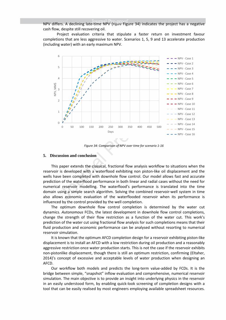
NPV differs. A declining late-time NPV (Figure Figure 34) indicates the project has a negative

cash flow, despite still recovering oil.

Project evaluation criteria that stipulate a faster return on investment favour

completions that are less aggressive to water. Scenarios 1, 5, 9 and 13 accelerate production

(including water) with an early maximum NPV.

Figure 34: Comparison of NPV over time for scenario 1-16

5. Discussion and conclusion

This paper extends the classical, fractional flow analysis workflow to situations when the

reservoir is developed with a waterflood exhibiting non piston-like oil displacement and the

wells have been completed with downhole flow control. Our model allows fast and accurate

prediction of the waterflood performance in both linear and radial cases without the need for

numerical reservoir modelling. The waterflood’s performance is translated into the time

domain using a simple search algorithm. Solving the combined reservoir-well system in time

also allows economic evaluation of the waterflooded reservoir when its performance is

influenced by the control provided by the well completion.

The optimum downhole flow control completion is determined by the water cut

dynamics. Autonomous FCDs, the latest development in downhole flow control completions,

change the strength of their flow restriction as a function of the water cut. This work’s

prediction of the water cut using fractional flow analysis for such completions means that their

fluid production and economic performance can be analysed without resorting to numerical

reservoir simulation.

It is known that the optimum AFCD completion design for a reservoir exhibiting piston-like

displacement is to install an AFCD with a low restriction during oil production and a reasonably

aggressive restriction once water production starts. This is not the case if the reservoir exhibits

non-pistonlike displacement, though there is still an optimum restriction, confirming (Eltaher,

2014)’s concept of excessive and acceptable levels of water production when designing an

AFCD.

Our workflow both models and predicts the long-term value-added by FCDs. It is the

bridge between simple, “snapshot” inflow evaluation and comprehensive, numerical reservoir

simulation. The main objective is to provide an insight into underlying physics in the reservoir

in an easily understood form, by enabling quick-look screening of completion designs with a

tool that can be easily realised by most engineers employing available spreadsheet resources.

0

1

2

3

4

5

6

0 50 100 150 200 250 300 350 400 450 500

NP

V,

MM

$

Days

NPV - Case 1

NPV - Case 2

NPV - Case 3

NPV - Case 4

NPV - Case 5

NPV - Case 6

NPV - Case 7

NPV - Case 8

NPV - Case 9

NPV - Case 10

NPV - Case 11

NPV - Case 12

NPV - Case 13

NPV - Case 14

NPV - Case 15

NPV - Case 16

This workflow can also be used to compare the numerical simulation as a means of validation,

pre-cursor, complementary tools to enhance the robustness of reservoir modelling alone.

Incorporating a description of the AWC’s performance into the waterflood analysis model

allows forecasting the down flow control configuration’s production profile, the oil recovery

and the economic gain. Our method is particularly useful for rapidly designing and optimising a

completion that maximizes a chosen criterion, e.g. oil recovery, economic value-added, etc.

The complexity of existing modelling tools ensures that this task is rarely examined in detail.

The reservoir sweep models forming the basis of these tools have been thoroughly

verified. They provide a simplified, fast, analysis of the impact of various well completion and

control options on the development and efficiency of a waterflood. The method’s

transparency and ease of implementation of its algorithms can make it a useful tool for well

and reservoir engineers.

6. Nomenclature

All values are in SI units and at reservoir conditions, unless otherwise stated.

A - effective area perpendicular to flow

a - flow control completion strength defined by

equation 14

b - formation volume factor

fw - fraction flow rate of water (watercut at

downhole conditions)

h - layer height k - horizontal permeability

L - distance between wells M - mobility ratio

n - exponent for modified Brooks-Corey

functions ΔP - pressure difference

P - pressure �1 – Capillary pressure

q - flow rate

re - The external reservoir radius (the peripheral

oil-water contact)

rf - The radius distance of the flood’s front rw - wellbore radius

S - saturation ΔS - movable saturation (1-Sor-Swi)

t - time u - fluid flow velocity

V - Cumulative liquid produced

x - The distance index for front advancement

evaluation between injector and producer

λ - fluid mobility (i.e. rel.perm./viscosity) t<"t#" = Fractional flow derivative

Subscripts

abt - after breakthrough avg - average

ann - annulus bt - breakthrough

bbt - before breakthrough e - external

f – denote the saturation or the location of

flood front Fcc – flow control completion

Injector – pressure drop occur at injector well j, k, R - referes to Layer j, k, or R respectively

Layer – pressure drop occur at layer N - Number of blocks with different water

saturations behind the flood front

n - the block’s index (behind the front) for

average relative permeability calculation o - oil

oh - Openhole or - residual oil (saturation)

Producer – pressure drop occur at producer

well r - relative (permeability)

s - The saturation index for postwater w - water

breakthrough evaluation

wi - irreducible water (saturation) wf - waterfront

Superscripts

a* - total FCC flow restriction coefficient for a layer, defined as a*=aproducer+ainjector

WI* - volume of water injected expressed in reservoir pore volumes

x* - relative water front position defined as x* = x/L

λ’ - end-point mobility

fw’ – derivative of fractional flow over water saturation

Abbreviations

AICD Autonomous Inflow Control Device (a class of FCDs)

AFCD Autonomous Flow Control Device (a class of FCDs)

AWC Advanced Well Completion

BL Buckley-Leverett

DP Dykstra-Parsons

DCF Discounted Cash Flow

EW Extended Welge

FCC Flow Control Completion (equivalent with FCD)

FCD Flow Control Device

FOE Field Oil Recovery

FOPT Field Oil Production Total (Cumulative oil production)

FWPT Field Water Production Total (Cumulative water production)

HA Harmonic Average

NPV Net Present Value

PV (reservoir) pore volume

Rcm (at) Reservoir conditions - cubic meters (units)

RE Oil Recovery Efficiency (recovery factor)

WI Volume of Water Injected

7. Acknowledgement

The authors thank the sponsor of the Value from Advanced Wells (VAWE) Joint-Industry

project at Heriot-Watt University for the support. The authors also thank Schlumberger

Information Solutions for the access to their software.

8. References

Ahmed, T. 2001, Reservoir Engineering Handbook (Second addition), Gulf Professional Pub.

ISBN: 0884157709, 9780884157700.

Al-Khelaiwi, Faisal T, Vasily M Birchenko, Michael R. Konopczynski et al. 2008. Advanced Wells:

A Comprehensive Approach to the Selection between Passive and Active Inflow Control

Completions. Presented at the International Petroleum Technology Conference, Kuala

Lumpur, Malaysia. IPTC- 12145-MS. https://doi.org/10.2523/IPTC-12145-MS

Al-Khelaiwi, 2013, A Comprehensive Approach to the Design of Advanced Well Completions.

PhD Thesis. Heriot-Watt University.

Birchenko, V. M., A. Iu Bejan, A. V. Usnich et al. 2011. Application of inflow control devices to

heterogeneous reservoirs (in Journal of Petroleum Science and Engineering 78 (2): 534-

541. http://dx.doi.org/10.1016/j.petrol.2011.06.022.

Brooks, R.H. and Corey, A.T., 1966. Properties of porous media affecting fluid flow. Journal of

the Irrigation and Drainage Division, 92(2), pp.61-90.

Buckley, S. E., & Leverett, M. C. (1942, December 1). Mechanism of Fluid Displacement in

Sands. Society of Petroleum Engineers. doi:10.2118/942107-G

Craig, F. F., Jr.1993, The Reservoir Engineering Aspects of Waterflooding, Monograph Series,

Richardson, Texas, SPE, (1993), 3.

Dake, L. 2001. The Practice of Reservoir Engineering (Revised Edition), Volume 36, ISBN:

9780080574431

Deppe, John C. 1961. Injection Rates - The Effect of Mobility Ratio, Area Swept, and Pattern.

SPE J 1 (02). https://doi.org/10.2118/1472-G

Dyes, A. B., B. H. Caudle, R. A. Erickson. 1954. Oil Production After Breakthrough as Influenced

by Mobility Ratio, SPE-309-G, http://dx.doi.org/10.2118/309-g.

Dykstra, H. and Parsons, R.L., 1950. The prediction of oil recovery by water flood. Secondary

recovery of oil in the United States, 2, pp.160-174.

El-Khatib, Noaman. 1985. The Effect of Crossflow on Waterflooding of Stratified Reservoirs

(includes associated papers 14490 and 14692 and 15043 and 15191). SPE J 25 (02). SPE

11495-pa. http://dx.doi.org/10.2118/11495-pa.

El-Khatib, Noaman. 1999. Waterflooding Performance of Communicating Stratified Reservoirs

With Log-Normal Permeability Distribution. SPE Res Eval & Eng 2 (06). SPE-59071-pa.

http://dx.doi.org/10.2118/59071-pa.

El-Khatib, Noaman A. 2012. Waterflooding Performance in Inclined Communicating Stratified

Reservoirs., Presented at the SPE North Africa Technical Conference and Exhibition, 14-

17 February, Cairo, Egypt. SPE-126344-ms. http://dx.doi.org/10.2118/126344-ms.

El-Khatib, Noaman A. F. 2003. Effect of Gravity on Waterflooding Performance of Stratified

Reservoirs. Presented at the SPE Middle East Oil Show, 9-12 June, Bahrain. SPE-81465-

ms, http://dx.doi.org/10.2118/81465-ms.

Eltaher, Eltazy Mohammed Khalid, Morteza Haghighat Sefat, Khafiz Muradov et al. 2014.

Performance of Autonomous Inflow Control Completion in Heavy Oil Reservoirs.

Presented at the International Petroleum Technology Conference, 10-12 December,

Kuala Lumpur, Malaysia. IPTC-17977-ms. https://doi.org/10.2523/IPTC-17977-MS

Eltazy Eltaher, Khafiz Muradov, David Davies, Peter Grassick, 2018. Autonomous flow control

device modelling and completion optimisation, Journal of Petroleum Science and

Engineering. https://doi.org/10.1016/j.petrol.2018.07.042

Goddin, C. S., Jr., F. F. Craig, Jr., J. O. Wilkes et al. 1966. A Numerical Study of Waterflood

Performance In a Stratified System With Crossflow. JPT 18 (06). SPE-1223-pa,


Haghighat Sefat, Morteza, Khafiz M. Muradov, Ahmed H. Elsheikh et al. 2016. Proactive

Optimization of Intelligent-Well Production Using Stochastic Gradient-Based Algorithms.

SPE Res Eval & Eng 19(02). SPE-178918-pa. http://dx.doi.org/10.2118/178918-pa.

Halliburton (2017), NETool List of publications. Halliburton

Henriksen, Knut Herman, Eli Iren Gule, Jody R. Augustine. 2006. Case Study: The Application of

Inflow Control Devices in the Troll Field. Presented at the SPE Europec/EAGE Annual

Conference and Exhibition, 12-15 June, Vienna, Austria. SPE-100308-MS.

http://dx.doi.org/10.2118/100308-ms.

Hiatt, W.N., 1958, January. Injected-fluid coverage of multi-well reservoirs with permeability

stratification. In Drilling and Production Practice. American Petroleum Institute.

Johnson, Carl E., Jr. 1956. Prediction of Oil Recovery by Waterflood - A Simplified Graphical

Treatment of the Dykstra-Parsons Method. JPT 8 (11). SPE-733-G.

http://dx.doi.org/10.2118/733-g.

Johnson, J. P. 1965. Predicting Waterflood Performance by the Graphical Representation of

Porosity and Permeability Distribution. SPE. doi:10.2118/918-PA

Ling, Kegang. 2012. Fractional Flow in Radial Flow System - A Study for Peripheral Waterflood.

Presented at the SPE Latin America and Caribbean Petroleum Engineering Conference,

16-18 April, Mexico City, Mexico. SPE-152129-MS. https://doi.org/10.2118/152129-MS

Ling, Kegang, 2016. Fractional flow in radial flow systems: a study for peripheral waterflood.

Journal of Petroleum Exploration and Production Technology 6 (03).

https://doi.org/10.1007/s13202-015-0197-3

Livescu, S., Brown, W. P., Jain, R., Grubert, M., Ghai, S. S., Lee, L.-B. W., & Long, T. 2010.

Application of a coupled wellbore/reservoir simulator to well performance optimization.

Presented at the SPE Annual Technical Conference and Exhibition, Florence, Italy. SPE-

135035-MS. https://doi.org/10.2118/135035-MS

Mijic, A., and T. C. LaForce (2012), Spatially varying fractional flow in radial CO2-brine

displacement,Water Resour. Res., 48, W09503, doi:10.1029/2011WR010961.

Muradov, K. M., Prakasa, B., & Davies, D. (2018, August 1). Extension of Dykstra-Parsons Model

of Stratified-Reservoir Waterflood To Include Advanced Well Completions. Society of

Petroleum Engineers. doi:10.2118/189977-PA

Muradov, K, Eltaher, E & Davies, DR 2018, 'Reservoir simulator-friendly model of fluid-

selective, downhole flow control completion performance' Journal of Petroleum Science

and Engineering, vol. 164, pp. 140-154. DOI: 10.1016/j.petrol.2018.01.039

Muscat, M. 1950. The effect of permeability stratification in complete water-drive systems (in

Trans., AIME: 349-358.)

Osman, Mohammed E., Djebbar Tiab. 1981. Waterflooding Performance and Pressure Analysis

Of Heterogeneous Reservoirs. Presented at the SPE Middle East Technical Conference

and Exhibition, 9-12 March, Bahrain. SPE-9656-MS. http://dx.doi.org/10.2118/9656-ms.

Prakasa, B., Muradov, K., & Davies, D. (2015, September 8). Rapid Design of an Inflow Control

Device Completion in Heterogeneous Clastic Reservoirs Using Type Curves. Society of

Petroleum Engineers. doi:10.2118/175448-MS

Prakasa, B, Muradov, K & Davies, DR 2019, 'Principles of rapid design of an Inflow Control

Device Completion in Homogeneous and Heterogeneous Reservoirs Using Type Curves'

Journal of Petroleum Science and Engineering, vol. 176, pp. 862-879. DOI:

10.1016/j.petrol.2019.01.104

Reznik, A. A., Robert M. Enick, Sudhir B. Panvelker. 1984. An Analytical Extension of the

Dykstra-Parsons Vertical Stratification Discrete Solution to a Continuous, Real-Time Basis

(includes associated papers 13753 and 13830 and 14873 and 14695). SPE J 24 (06).


Rossen, W.R., Johns, R.T., Kibodeaux, K.R., Lai, H. and Tehrani, N.M., 2008, September.

Fractional-flow theory applied to non-Newtonian IOR processes. In ECMOR XI-11th

European Conference on the Mathematics of Oil Recovery.

Snyder, R. W., H. J. Ramey, Jr. 1967. Application of Buckley-Leverett Displacement Theory to

Non-communicating Layered Systems, JPT 19 (11). http://dx.doi.org/10.2118/1645-pa.

Warren, J. E. 1964. Prediction of Waterflood Behavior in a Stratified System. SPE J 4 (02).


Welge, H., “A Simplified Method for Computing Oil Recovery by Gas or Water Drive,” Trans.

AIME, 1952, pp. 91–98. Williams, G. J. J., Mansfield, M., MacDonald, D. G., & Bush, M. D. 2004. Top-Down Reservoir

Modelling. Presented at the SPE Annual Technical Conference and Exhibition, Houston,

U.S.A. SPE-89974-MS. https://doi.org/10.2118/89974-MS.

Wu, Y.-S., Fakcharoenphol, P., & Zhang, R. (2010, January 1). Non-Darcy Displacement in Linear

Composite and Radial Flow Porous Media. Society of Petroleum Engineers.

doi:10.2118/130343-MS

Zhang, H., Ling, K., & Acura, H. (2013, April 15). New Analytical Equations of Recovery Factor

for Radial Flow Systems. Society of Petroleum Engineers. doi:10.2118/164766-MS

Linear and radial flow modelling of a waterflooded, stratified, non-communicating

reservoir developed with downhole, flow control completions

Highlight

This manuscript presents a new approach to model reservoirs with Advanced

Well Completion (AWC) that enables fast design of AWC and complements the

operators’ existing workflows. The fluid flow through the reservoir-AWC-well system

is characterised as a much simpler proxy model (reduced-physics model), that is still

comprehensive enough to capture the main characteristic of the reservoir system. It

provides a simple model, that is appropriate to the available data, while hence

allowing a quick scoping of concepts and options prior, or in addition, to detailed

reservoir modelling. Such workflows meet the oil and gas business’s preferences for

simpler and faster processes.

A simple, portable toolbox is coded to determine the optimal completion

response in various field/fluid conditions within the short time that is available when

making a decision. Furthermore, the proposed proxy models could be enrolled as a

fast initiation (or quick scoping) prior, or in addition, to detailed modelling enabling a

faster work cycle.

We aims to develop a framework that enables to design ICD and AFCD

completion for long-term optimisation, i.e. in the ‘dynamic’ reservoir flow condition.

The chapter starts by providing the advantage of having a long-term

strategy/outlook when designing the flow control completion. The feasibility of AWC

is mainly influenced by the economic parameters, which can only be obtained once

we have an outlook on the long-term results from installing the AWC. The developed

model is constructed from the combination of classical waterflood displacement

equations with a recently developed analytical model of a flow control completion.

The idea is then extended for light-oil displacement, which replicates piston-like

displacement (an extension of Dykstra-Parsons solution to AWC wells) and

medium/heavy-oil displacement, which replicate non-piston like displacement (an

extension of Buckley-Leverett & Welge solution to AWC wells). The model was

successfully tested and verified using numerical reservoir simulation.

linear and radial flow modelling of a waterflooded

Documents